Know When to Abstain: Optimal Selective Classification with Likelihood Ratios

Abstract

Selective classification enhances the reliability of predictive models by allowing them to abstain from making uncertain predictions. In this work, we revisit the design of optimal selection functions through the lens of the Neyman–Pearson lemma, a classical result in statistics that characterizes the optimal rejection rule as a likelihood ratio test. We show that this perspective not only unifies the behavior of several post-hoc selection baselines, but also motivates new approaches to selective classification which we propose here. A central focus of our work is the setting of covariate shift, where the input distribution at test time differs from that at training. This realistic and challenging scenario remains relatively underexplored in the context of selective classification. We evaluate our proposed methods across a range of vision and language tasks, including both supervised learning and vision-language models. Our experiments demonstrate that our Neyman–Pearson-informed methods consistently outperform existing baselines, indicating that likelihood ratio-based selection offers a robust mechanism for improving selective classification under covariate shifts. Our code is publicly available at https://github.com/clear-nus/sc-likelihood-ratios.

1 Introduction

Machine learning models are inherently fallible and can make erroneous predictions. Unlike humans, who can abstain from answering when uncertain, e.g., by saying “I don’t know”, predictive models typically produce a prediction for every input regardless of confidence. Selective classification aims to address this limitation by enabling models to abstain on uncertain inputs, thereby improving overall performance and robustness, for instance by deferring ambiguous cases to human experts.

A wide range of methods have been proposed to determine whether a model should accept or reject an input. Common post-hoc approaches rely on heuristic confidence estimates, such as the maximum softmax probability Geifman and El-Yaniv [2017], Hendrycks and Gimpel [2017], logit margins Liang et al. [2024], or Monte Carlo dropout Geifman and El-Yaniv [2017], Gal and Ghahramani [2016]. Other techniques assess a sample’s proximity to the training distribution Lee et al. [2018], Sun et al. [2022], under the assumption that samples farther from the data manifold are more likely to be misclassified. A separate line of work trains models with explicit abstention mechanisms, such as a rejection logit or head Geifman and El-Yaniv [2019], Liu et al. [2019], Huang et al. [2020]. In this work we focus on post-hoc methods, which are model-agnostic and do not require specialized training.

Despite the rich literature, two important gaps remain. First, while foundational results (such as Chow [1970], Geifman and El-Yaniv [2017]) provide theoretical underpinnings for selective classification, there is a lack of general, principled guidance for designing effective selector functions in the context of modern deep networks. Second, most evaluations are conducted in the i.i.d. setting, where test data is assumed to follow the training distribution. This setup fails to reflect challenges in real-world scenarios, where distribution shifts, especially covariate shifts, are common, reducing the practical relevance of existing results.

To address these challenges, we propose a new perspective rooted in the Neyman–Pearson lemma, a classical result from statistics that defines the optimal hypothesis test in terms of a likelihood ratio. We show that existing selectors can be interpreted as approximations to this test, and we use this insight to derive two new selectors, $\Delta$-MDS and $\Delta$-KNN, as well as a simple linear combination strategy. We evaluate our methods on a comprehensive suite of vision and language benchmarks under covariate shift, where the input distribution changes while the label space remains fixed. We focus on covariate shift for two key reasons: first, it is underexplored relative to semantic shifts Heng and Soh [2025] (which is well studied in the context of out-of-distribution detection Hendrycks and Gimpel [2017], Ming et al. [2022], Lee et al. [2018], Heng et al. [2024]); second, it is increasingly relevant in modern applications such as vision-language models (VLMs), where the label set is large and variable, rendering most practical shifts in deployment covariate in nature. Our results demonstrate that the proposed selectors outperform existing baselines and provide robust performance across distribution shifts, including on powerful VLMs like CLIP.

In summary, our key contributions are:

1. We introduce for the first time a Neyman–Pearson-based framework for defining optimality in selective classification via likelihood ratio tests.

2. We unify several existing selector methods and propose two new selectors and a linear combination approach under this framework.

3. We conduct a thorough evaluation under covariate shift across vision and language tasks and demonstrate superior performance across both VLMs and traditional supervised models.

2 Background

Selective Classification.

Consider a standard classification problem with input space $\mathcal{X}\subseteq\mathbb{R}^{d}$, label space $\mathcal{Y}=\{1,...,K\}$, and data distribution $\mathcal{D}_{\mathcal{X},\mathcal{Y}}$ over $\mathcal{X}\times\mathcal{Y}$. A selective classifier is a pair $(f,g)$, where $f:\mathcal{X}\rightarrow\mathbb{R}^{K}$ is a base classifier, and $g:\mathcal{X}\rightarrow\{0,1\}$ is a selector function that determines whether to make a prediction or abstain. Formally,

$$(f,g)({\bm{x}})\triangleq\begin{cases}f({\bm{x}})&\text{if }g({\bm{x}})=1,\\ \text{abstain}&\text{if }g({\bm{x}})=0.\end{cases}$$ (1)

That is, the model abstains on input ${\bm{x}}$ when $g({\bm{x}})=0$. In practice, $g$ is typically implemented by thresholding a real-valued confidence score:

$$g_{s,\gamma}({\bm{x}})=\mathbbm{1}[s({\bm{x}})>\gamma],$$ (2)

where $s:\mathcal{X}\rightarrow\mathbb{R}$ is a confidence scoring function (often adapted from OOD detection methods; see below), and $\gamma$ is a tunable threshold.

The performance of a selective classifier is typically evaluated using two metrics:

Coverage: $$\phi_{s,\gamma}=\mathbb{E}_{{\bm{x}}\sim\mathcal{D}_{\mathcal{X},\mathcal{Y}}}[g_{s,\gamma}({\bm{x}})],$$ (3)

Selective Risk: $$R_{s,\gamma}=\frac{\mathbb{E}_{({\bm{x}},y)\sim\mathcal{D}_{\mathcal{X},\mathcal{Y}}}[\ell(f({\bm{x}}),y)\cdot g_{s,\gamma}({\bm{x}})]}{\phi_{s,\gamma}},$$ (4)

where $\ell(f({\bm{x}}),y)$ is the 0/1 loss Geifman and El-Yaniv [2017]. Selective classification aims to optimize the tradeoff between selective risk and coverage by ideally reducing risk while maintaining high coverage. Improvements can stem from enhancing the base classifier $f$, or from refining the selector $g$ to better identify error-prone inputs. In this work, we fix $f$ to be a strong pretrained model and focus on designing more effective selector functions $g$.

Covariate Shift.

Covariate shift refers to a scenario where the marginal distribution over inputs, $p({\bm{x}})$, changes between training and testing, while the label distribution $p(y)$ remains unchanged. For example, a model trained on photographs of cats may face a covariate shift when evaluated on paintings of cats, as the input appearance changes but the semantic categories are preserved. This is in contrast to semantic shift, where both $p({\bm{x}})$ and $p(y)$ change, typically due to the introduction of unseen classes. In this work, we focus on covariate shifts, which are increasingly relevant in modern applications such as VLMs, where the label set is large and can be adjusted to suit a given task. In such settings, distributional changes primarily manifest as covariate shifts, making them a critical yet underexplored challenge for robust selective classification.

Out-of-Distribution (OOD) Detection.

OOD detection is closely related to selective classification, as many selector functions $s({\bm{x}})$ are derived from or inspired by OOD scoring methods. Given an in-distribution (ID) data distribution $p_{ID}$, the goal of OOD detection is to construct a scoring function $s:\mathcal{X}\rightarrow\mathbb{R}$ such that $s({\bm{x}})$ indicates the likelihood that ${\bm{x}}$ originates from $p_{ID}$. A higher $s({\bm{x}})$ corresponds to higher confidence that ${\bm{x}}$ is in-distribution. In selective classification, these scores are thresholded to determine whether to accept or abstain on a given input, as formalized in Eq. 2.

3 Selective Classification via the Neyman–Pearson Lemma

We begin by framing selective classification within the classical paradigm of hypothesis testing. Let $\mathcal{H}_{0}:\mathcal{C}$ denote the hypothesis that the classifier makes a correct prediction, and $\mathcal{H}_{1}:\neg\mathcal{C}$ the hypothesis that it makes an incorrect one. Selective classification then reduces to deciding, for each input, whether to accept $\mathcal{H}_{0}$ or reject it in favor of $\mathcal{H}_{1}$, i.e., a binary decision problem. This perspective is a natural fit for a foundational result from statistics: the Neyman–Pearson (NP) lemma [Neyman and Pearson, 1933, Lehmann et al., 1986], which characterizes the optimal decision rule between two competing hypotheses.

Lemma 1 (name=Neyman–Pearson Neyman and Pearson [1933], Lehmann et al. [1986]).

Let $Z\in\mathbb{R}^{d}$ be a random variable, and consider the hypotheses:

$$\mathcal{H}_{0}:Z\sim P_{0}\quad\text{vs.}\quad\mathcal{H}_{1}:Z\sim P_{1},$$

where $P_{0}$ and $P_{1}$ have densities $p_{0}$ and $p_{1}$ that are strictly positive on a shared support $\mathcal{Z}\subset\mathbb{R}^{d}$. For any measurable acceptance region $A\subset\mathcal{Z}$ under $\mathcal{H}_{0}$, define the type I error (false rejection) as $\alpha(A)=P_{0}(Z\notin A)$, and type II error (false acceptance) as $\beta(A)=P_{1}(Z\in A)$.

Fix a type I error tolerance $\alpha_{0}\in[0,1]$. Let $\gamma(\alpha_{0})$ be the threshold such that

$$A^{*}(\alpha_{0}):=\left\{z\in\mathcal{Z}:\frac{p_{0}(z)}{p_{1}(z)}\geq\gamma(\alpha_{0})\right\}$$

satisfies $\alpha(A^{*})=\alpha_{0}$. Then $A^{*}(\alpha_{0})$ minimizes the type II error:

$$\beta(A^{*}(\alpha_{0}))=\min_{A:\alpha(A)=\alpha_{0}}\beta(A).$$

In other words, among all decision rules with the same false rejection rate, the likelihood ratio test minimizes the false acceptance rate.

Applied to selective classification, Lemma 1 implies that the optimal selection score takes the form of a likelihood ratio:

$$s({\bm{x}})=\frac{p_{c}({\bm{x}})}{p_{w}({\bm{x}})},$$

where $p_{c}({\bm{x}})$ and $p_{w}({\bm{x}})$ denote the probability densities of the classifier making a correct and wrong prediction respectively. Thresholding this score yields the lowest possible selective risk for any given coverage level.

Corollary 1 (name=Informal).

Any selector score $s({\bm{x}})$ that is a monotonic transformation of the likelihood ratio $\frac{p_{0}({\bm{x}})}{p_{1}({\bm{x}})}$ is also optimal under the Neyman–Pearson criterion.

Corollary 1 follows directly from the lemma, since monotonic transformations (e.g., logarithmic or affine maps) preserve the ordering of scores and hence do not alter the resulting acceptance region. We define a score function $s({\bm{x}})$ to be Neyman–Pearson optimal if it is a monotonic transformation of the likelihood ratio $p_{c}({\bm{x}})/p_{w}({\bm{x}})$. In practice, the true likelihood ratio is not accessible, so we approximate it or construct a monotonic proxy that captures the posterior odds of a correct versus incorrect prediction for a given input. In what follows, we first reinterpret existing selection scores from the literature as implicit approximations to this likelihood ratio and show conditions under which they are NP optimal. We then introduce two new distance-based selection functions directly inspired by the NP framework. Finally, we propose a hybrid score that linearly combines multiple selectors which we find performs well in practice.

3.1 Logit-Based Scores as Approximations to Likelihood Ratios

We begin by revisiting two popular confidence scores in classification, Maximum Softmax Probability (MSP) [Hendrycks and Gimpel, 2017] and Raw Logits (RLog) [Liang et al., 2024], and show that both can be interpreted as approximations to likelihood ratio tests in the sense of the NP lemma. This provides a theoretical justification for their empirical success as selection functions in selective classification.

Let $l^{(1)}\geq l^{(2)}\geq\cdots\geq l^{(K)}$ denote the logits output by a classifier for a sample ${\bm{x}}$, sorted in descending order. Define the corresponding softmax probabilities $d^{(i)}=\mathrm{softmax}(l^{(i)})$. The MSP score is given by $s_{\mathrm{MSP}}({\bm{x}})=d^{(1)}$, while the RLog score is defined as $s_{\mathrm{RLog}}({\bm{x}})=l^{(1)}-l^{(2)}$. MSP has become a standard baseline for OOD detection and selective classification [Hendrycks and Gimpel, 2017, Geifman and El-Yaniv, 2017], and RLog has been recently proposed as a strong score for selective classification [Liang et al., 2024].

Theorem 1.

Assume the classifier is calibrated in the sense that $P(Y=k\mid p_{\theta}(y=k\mid{\bm{x}})=\hat{p})=\hat{p}$ [Guo et al., 2017]. Then MSP is Neyman–Pearson optimal for selective classification. Moreover, under the additional assumption that the softmax distribution is concentrated on the top two classes, i.e., $L:=\sum_{i\geq 3}d^{(i)}\ll d^{(2)}$, the RLog score is also Neyman–Pearson optimal.

The proof provided in Appendix A shows that under these assumptions, both MSP and RLog are monotonic transformations of the likelihood ratio $p_{c}/p_{w}$, and therefore is NP optimal by Corollary 1. Of course, these assumptions are not always satisfied in practice. Prior work [Guo et al., 2017] has shown that modern neural classifiers tend to be poorly calibrated, and has proposed post-hoc calibration methods such as temperature scaling. Notably, RLog has been shown to be invariant to temperature scaling [Liang et al., 2024], making it robust to miscalibration and a compelling choice in practice. This aligns with our empirical findings in Sec. 5, where RLog generally outperforms MSP (which corresponds to temperature scaling with $T=1$). While the effect of calibration is an important factor in logit-based selective classification methods Cattelan and Silva [2023], Fisch et al. [2022], it lies beyond the scope of this work.

3.2 Neyman–Pearson Optimal Distance Scores

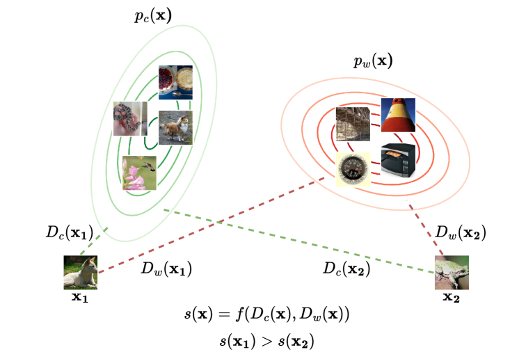
Figure 1: Illustration of our proposed Neyman–Pearson optimal distance-based selective classification methods. We estimate the likelihoods of correct and incorrect predictions ($p_{c}$ and $p_{w}$) as a function of distances to training sets consisting of correctly and incorrectly classified samples: $s({\bm{x}})=f(D_{c}({\bm{x}}),D_{w}({\bm{x}}))$, where $f$ here denotes a function. For example, ${\bm{x}}_{1}$ is “closer” to $p_{c}$ and “farther” from $p_{w}$ than ${\bm{x}}_{2}$, and should therefore receive a higher score.

The logit-based scores discussed in the previous section rely on classifier logit calibration, a condition often violated in practice [Guo et al., 2017]. To avoid this dependency, we consider distance-based methods that make alternative assumptions independent of calibration. As we show below, these methods approximate the likelihood ratio $p_{c}/p_{w}$ by leveraging spatial relationships in feature space.

Two distance methods widely used in OOD detection are the Mahalanobis distance (MDS) [Lee et al., 2018] and $k$-Nearest Neighbors (KNN) [Sun et al., 2022]. Both rely on computing distances between a test sample and training features. Specifically, MDS is defined as $s_{\text{MDS}}({\bm{x}})=\max_{i}-(\phi({\bm{x}})-\mu_{i})^{\top}\Sigma^{-1}(\phi({\bm{x}})-\mu_{i})$, where $\phi({\bm{x}})$ denotes the extracted feature of ${\bm{x}}$, typically from the penultimate or final layer of a trained deep network, $\mu_{i}$ is the empirical mean feature of class $i$, and $\Sigma$ is a shared covariance matrix. In contrast, KNN scores inputs by the negative distance to the $k$-th nearest training feature vector. We introduce $\Delta$-MDS and $\Delta$-KNN, which are modified versions of these scores that explicitly incorporate insights from the NP lemma by estimating separate distributions for correctly and incorrectly classified training samples. Figure 1 gives an overview of our approach, and we provide pseudocode for our proposed methods in Appendix C.

$\Delta$-MDS.

Instead of estimating a single distribution per class, we maintain two sets of statistics per class: $\{\mu_{i}^{c},\Sigma^{c}\}_{i=1}^{K}$ and $\{\mu_{i}^{w},\Sigma^{w}\}_{i=1}^{K}$, corresponding to the mean and shared covariance of features for training samples that the classifier predicts correctly and wrongly, respectively. These quantities are easily estimated as the true labels are known. We then define the $\Delta$-MDS score as the difference in Mahalanobis distances between the two distributions:

$$s_{\Delta\text{-MDS}}({\bm{x}})=D_{\text{MDS}}({\bm{x}};\mu_{i}^{c},\Sigma^{c})-D_{\text{MDS}}({\bm{x}};\mu_{i}^{w},\Sigma^{w})$$ (5)

where $D_{\text{MDS}}({\bm{x}};\mu_{i},\Sigma)=\max_{i}-(\phi({\bm{x}})-\mu_{i})^{\top}\Sigma^{-1}(\phi({\bm{x}})-\mu_{i})$ is the standard Mahalanobis score. The score intuitively increases when the input is closer (in Mahalanobis sense) to the “correctly classified” region and farther from the “wrongly classified” region in feature space. We now formalize this intuition:

Theorem 2.

Let $Z=\phi({\bm{x}})\in\mathbb{R}^{d}$ be the feature representation of input ${\bm{x}}$. Let $\mathcal{C}$ be the event the classifier makes a correct prediction and $\neg\mathcal{C}$ its negation. Assume $Z|\mathcal{C}\sim p_{c}=\mathcal{N}(\mu_{i}^{c},\Sigma^{c})$ and $Z|\neg\mathcal{C}\sim p_{w}=\mathcal{N}(\mu_{i}^{w},\Sigma^{w})$. Then the $\Delta$-MDS score $s_{\Delta\text{-MDS}}({\bm{x}})$ is Neyman–Pearson optimal for selective classification.

The proof is provided in Appendix A, which shows that $s_{\Delta\text{-MDS}}$ is a monotonic transformation of the likelihood ratio $p_{c}/p_{w}$, and thus is NP optimal as per Corollary 1. The Gaussian assumption on feature representations is supported both empirically and theoretically via connections between Gaussian Discriminant Analysis and softmax classifiers [Lee et al., 2018], making $\Delta$-MDS well-suited for modern deep classifiers trained on standard supervised learning objectives.

$\Delta$-KNN.

Next we introduce $\Delta$-KNN, a non-parametric distance-based score inspired by the NP framework. Let $A_{c}=\{\phi_{c}({\bm{x}}_{1}),\dots,\phi_{c}({\bm{x}}_{N_{c}})\}$ and $A_{w}=\{\phi_{w}({\bm{x}}_{1}),\dots,\phi_{w}({\bm{x}}_{N_{w}})\}$ denote the feature representations of training samples that the classifier predicted correctly and wrongly respectively, and $N_{c}=|A_{c}|$ and $N_{w}=|A_{w}|$. Let ${\bm{z}}=\phi({\bm{x}})$ be the feature vector of a test input ${\bm{x}}$. Define $u_{k}({\bm{z}})$ and $v_{k}({\bm{z}})$ as the Euclidean distances from ${\bm{z}}$ to its $k$-th nearest neighbors in $A_{c}$ and $A_{w}$. We define the $\Delta$-KNN score as the difference in log-distances:

$$s_{\Delta\text{-KNN}}({\bm{x}})=D_{\text{KNN}}({\bm{x}};A_{c})-D_{\text{KNN}}({\bm{x}};A_{w})$$ (6)

where $D_{\text{KNN}}({\bm{x}};A_{c})=-\log[u_{k}(\phi({\bm{x}}))]$ and $D_{\text{KNN}}({\bm{x}};A_{w})=-\log[v_{k}(\phi({\bm{x}}))]$. This score measures how much closer a test point is to the region of correctly classified samples compared to incorrectly classified ones. We now show that $\Delta$-KNN is asymptotically NP optimal:

Theorem 3.

Let $Z=\phi({\bm{x}})\in\mathbb{R}^{d}$ be the feature representation of input ${\bm{x}}$, and let $\mathcal{C}$ denote the event that the classifier makes a correct prediction. Suppose $Z\mid\mathcal{C}\sim p_{c}$ and $Z\mid\neg\mathcal{C}\sim p_{w}$ are arbitrary continuous densities bounded away from zero. Let $N_{c}=|A_{c}|$ and $N_{w}=|A_{w}|$. If $k\to\infty$ while $k/N_{c}\to 0$ and $k/N_{w}\to 0$ as $N_{c},N_{w}\to\infty$, then $s_{\Delta\text{-KNN}}({\bm{x}})$ is a Neyman–Pearson optimal selector.

The proof is provided in Appendix A. As in previous cases, it relies on showing that $s_{\Delta\text{-KNN}}$ is a monotonic transformation of the likelihood ratio $p_{c}/p_{w}$. Importantly, this result does not require parametric assumptions on the form of $p_{c}$ or $p_{w}$, unlike $\Delta$-MDS. However, it does depend on asymptotic properties of the $k$-nearest neighbor density estimator, and the required conditions on $k$, $N_{c}$, and $N_{w}$ may be difficult to satisfy in finite-sample settings. As such, both methods have their tradeoffs in terms of modeling assumptions.

In practice, we replace the single $k$-th neighbor distance with the average log-distance to the top $k$ neighbors. Specifically, we use: $D_{\text{KNN}}({\bm{x}};A_{c})=-\frac{1}{k}\sum_{i=1}^{k}\log[u_{i}(\phi({\bm{x}}))]$ and $D_{\text{KNN}}({\bm{x}};A_{w})=-\frac{1}{k}\sum_{i=1}^{k}\log[v_{i}(\phi({\bm{x}}))]$. We find that this smoother version improves empirical performance, as shown in our ablation studies in Sec. 5.3. While this modification deviates from the form in Theorem 3, we include a discussion in Appendix B suggesting NP optimality holds for the averaged log-distance formulation under standard assumptions.

3.3 Linear Combinations Of Distance and Logit-based Scores

The selector scores we have introduced rely on different modeling assumptions and exhibit complementary strengths. Logit-based scores utilize the classifier’s learned boundaries, while distance-based methods depend on geometric structures in feature space defined by training samples. This observation motivates a natural question: can we combine these scores to leverage their respective advantages? We answer in the affirmative by proposing a simple yet effective solution: linearly combining selector scores. Intuitively, this allows each score to compensate for the limitations of the other. The following lemma formalizes the NP optimality of such a linear combination:

Lemma 2.

Let $s_{1}({\bm{x}})\in\mathbb{R}$ and $s_{2}({\bm{x}})\in\mathbb{R}$ be two selector scores. Assume both are Neyman–Pearson optimal; that is, $s_{1}({\bm{x}})$ is a monotone transform of $p_{c}^{(1)}/p_{w}^{(1)}$ and $s_{2}({\bm{x}})$ is a monotone transform of $p_{c}^{(2)}/p_{w}^{(2)}$. Then for any scalar $\lambda\in\mathbb{R}$, $t({\bm{x}})=s_{1}({\bm{x}})+\lambda s_{2}({\bm{x}})$ is a monotonic transformation of $p_{c}^{(1)}(p_{c}^{(2)})^{\lambda}/p_{w}^{(1)}(p_{w}^{(2)})^{\lambda}$.

The proof provided in Appendix A follows by expressing $t({\bm{x}})$ as a log-product of likelihood ratios. Thus, $t({\bm{x}})$ remains NP optimal under the assumption that the density for each hypothesis takes the form of a multiplicative (or “tilted”) product: $p_{c}^{(1)}(p_{c}^{(2)})^{\lambda}/Z_{c}$ and similarly for $p_{w}$, where $Z_{c}$ is a normalization constant. In practice, we find that combining a distance-based score (e.g., $\Delta$-MDS) with a logit-based score (e.g., RLog) leads to the best performance. We refer to such combinations by concatenating their names, e.g., $\Delta$-MDS-RLog. While the mixing coefficient $\lambda$ can be determined via grid search, we observe that balancing the magnitudes of $s_{1}({\bm{x}})$ and $s_{2}({\bm{x}})$ yields the best results without requiring extensive tuning.

4 Related Works

The study of classification with a reject option is long-standing. Early foundational works considered cost-based rejection models Chow [1970], as well as in classical machine learning paradigms such as support vector machines Fumera and Roli [2002], Bartlett and Wegkamp [2008] and nearest neighbor estimators Hellman [1970]. In the context of deep learning, LeCun et al. [1989] was among the first to examine rejection based on the top logits’ activations in image classification. A modern treatment of selective classification was later developed El-Yaniv et al. [2010], Geifman and El-Yaniv [2017], introducing the key concepts of classifier–selector pairs and the risk–coverage trade-off, which underpin our framework. Geifman and El-Yaniv [2017] further proposed a method for achieving guaranteed risk bounds and evaluated selection strategies based on model confidence scores, such as softmax response (equivalent to MSP) and Monte Carlo dropout Gal and Ghahramani [2016]. These approaches share the underlying assumption that confidence estimates are well-calibrated indicators of predictive correctness.

Subsequent works have extended this direction by studying popular logit and distance-based scores, many originally developed for OOD detection. Notable examples include MSP Hendrycks and Gimpel [2017], MaxLogit Hendrycks et al. [2019], Energy Liu et al. [2020], MDS Lee et al. [2018], and KNN Sun et al. [2022]. A critical limitation of logit-based methods is their reliance on classifier calibration. Although calibration is not the focus of our work, several studies have examined its impact on selective classification performance Cattelan and Silva [2023], Galil et al. [2023]. Related to this, conformal prediction provides an alternative framework for producing calibrated confidence or prediction sets with formal coverage guarantees Vovk et al. [2005], Angelopoulos and Bates [2021], Bates et al. [2021], Angelopoulos et al. [2024]. While such methods could in principle be adapted for selective classification, they differ fundamentally from our goal of designing scoring functions optimized for selective risk.

Beyond post-hoc methods, training-time approaches have been proposed where models are explicitly designed with a reject option. For example, SelectiveNet Geifman and El-Yaniv [2019] incorporates a rejection head and jointly trains the model to both classify and reject. Similarly, Deep Gamblers Liu et al. [2019] and Self-Adaptive Training Huang et al. [2020] reformulate $K$-way classification into $K+1$ classes by introducing an explicit reject class. These methods differ from ours in that they require architectural modifications and joint training. In contrast, we focus on post-hoc methods that can be applied to any pretrained classifier without retraining. This enhances applicability in practice, where most deployed models do not include rejection mechanisms by design.

Most closely related to our work is Liang et al. [2024], who study selective classification under general distribution shifts, which include both semantic and covariate shifts. They also introduce the Raw Logit (RLog) score, which we analyze in this work. Our work differs in several key ways: 1) we focus specifically on covariate shifts, which we argue is more relevant in modern settings where large and variable label sets (e.g., from vision-language models) mitigate label drift; 2) we introduce a unified theoretical framework grounded in the Neyman–Pearson lemma, from which we derive new selector scores with formal optimality guarantees; and 3) we evaluate our methods on a broader class of models, including VLMs, whereas Liang et al. [2024] focus exclusively on standard supervised learning paradigms.

5 Experiments

Datasets.

We evaluate our methods across vision and language domains, with a primary focus on the former. For vision tasks, we use ImageNet-1K (Im-1K) and a suite of covariate-shifted variants: 1) ImageNet-Rendition (Im-R) [Hendrycks et al., 2020], 2) ImageNet-A (Im-A) [Hendrycks et al., 2021], 3) ObjectNet (ON) [Barbu et al., 2019], 4) ImageNetV2 (Im-V2) [Recht et al., 2019], 5) ImageNet-Sketch (Im-S) [Wang et al., 2019], and 6) ImageNet-C (Im-C) [Hendrycks and Dietterich, 2019]. We group these datasets based on label coverage: full 1000-class coverage (Im-1K, Im-V2, Im-S, Im-C) and subsets of classes (Im-R, Im-A, ON). For language tasks, we evaluate on the Amazon Reviews dataset [Ni et al., 2019, Koh et al., 2021]. To simulate realistic deployment scenarios involving distribution shift, following Liang et al. [2024] we evaluate on mixed test sets that combine in-distribution and covariate-shifted samples. For example, results reported on Im-C are computed on a combined test set of Im-1K and Im-C.

Classifiers and Baseline Selector Scores.

For vision experiments, we consider two families of classifiers, CLIP-based zero-shot VLMs Radford et al. [2021] and supervised classifiers. Specifically, we use the CLIP model from Data Filtering Networks (DFN) Fang et al. [2024] and EVA Fang et al. [2023] for supervised learning, chosen for their state-of-the-art accuracy on ImageNet. Our focus is not on model training but on evaluating selector scores applied post-hoc. Note that for EVA, we restrict evaluation to datasets with full 1K class coverage as the model is trained on the complete ImageNet label set only. In contrast, CLIP can be adapted at inference time to arbitrary label subsets, so we evaluate it across all datasets. For language tasks, we fine-tune a DistilBERT Sanh et al. [2019] model using LISA Yao et al. [2022] on the Amazon Reviews training set and evaluate selective classification performance on the full test set.

In terms of baseline selector scores, we compare our proposed selector scores $\Delta$-MDS, $\Delta$-KNN, and their linear combinations with commonly used OOD detection and uncertainty-based scores: MSP [Hendrycks and Gimpel, 2017], MCM (for CLIP), MaxLogit [Hendrycks et al., 2019], Energy [Liu et al., 2020], MDS [Lee et al., 2018], KNN [Sun et al., 2022], and RLog [Liang et al., 2024]. As they are functionally similar, we will abbreviate MCM as MSP when presenting CLIP results for simplicity. Detailed experimental settings are provided in Appendix D.

Evaluation Metrics.

We evaluate performance using two metrics: the Area Under the Risk-Coverage Curve (AURC) and the Normalized AURC (NAURC) Cattelan and Silva [2023]. The AURC captures the joint performance of the classifier and selector across coverage levels. NAURC normalizes AURC to account for the classifier’s base error rate, providing a fairer comparison across models with different accuracies. Formally, NAURC is defined as:

$$\text{NAURC}(f,g)=\frac{\text{AURC}(f,g)-\text{AURC}(f,g^{*})}{R(f)-\text{AURC}(f,g^{*})},$$ (7)

where $g^{*}$ denotes an oracle confidence function achieving optimal AURC, and $R(f)$ is the risk of $f$. Intuitively, NAURC measures how close the selector $g$ gets to the optimal, normalized by the classifier’s total error. Thus, while AURC is useful for understanding overall performance in the context of a specific model, NAURC enables fair selector comparisons across models by factoring out baseline classifier accuracy.

5.1 Image Experiments

Table 1: DFN CLIP AURC (A) and NAURC (N) results on ImageNet and its covariate shifted variants at full coverage. Lower is better. AURC results are on the $10^{-2}$ scale. Bold and underline denotes the best and second best result respectively. “Avg (1K)" denotes average results over datasets with full 1K-class coverage, while “Avg (all)" is the average result over all datasets.

	Im-1K		Im-R		Im-A		ON		Im-V2		Im-S		Im-C		Avg (1K)		Avg (all)
Method	A	N	A	N	A	N	A	N	A	N	A	N	A	N	A	N	A	N
MSP	9.08	0.542	2.00	0.344	2.29	0.179	8.87	0.268	9.39	0.521	12.3	0.524	15.1	0.328	11.5	0.479	8.43	0.387
MaxLogit	9.08	0.542	2.21	0.385	2.96	0.249	12.4	0.437	9.35	0.518	12.3	0.525	17.7	0.423	13.9	0.502	11.3	0.440
Energy	14.2	0.901	5.81	1.06	12.2	1.2	33.3	1.43	14.9	0.882	20.8	0.975	49.2	1.59	24.8	1.09	21.5	1.15
MDS	11.3	0.699	3.41	0.608	3.21	0.274	16.4	0.624	11.7	0.672	15.2	0.68	17.6	0.426	13.9	0.619	11.3	0.569
KNN	10.5	0.643	2.51	0.439	2.67	0.219	11.4	0.390	10.9	0.618	14.1	0.619	16.7	0.389	13.1	0.567	9.83	0.474
RLog	4.83	0.246	0.808	0.122	1.59	0.108	7.73	0.214	5.27	0.250	6.84	0.234	12.6	0.226	7.39	0.239	5.67	0.200
$\Delta$-MDS	5.00	0.257	2.19	0.380	2.43	0.194	9.63	0.304	5.43	0.260	8.28	0.311	12.5	0.224	7.81	0.263	6.50	0.276
$\Delta$-KNN	4.60	0.230	1.42	0.237	1.99	0.149	8.52	0.252	4.99	0.231	7.55	0.272	12.1	0.207	7.32	0.235	5.89	0.225
$\Delta$-MDS-RLog	4.13	0.197	1.09	0.175	1.60	0.109	7.13	0.185	4.52	0.200	6.27	0.204	11.1	0.170	6.51	0.193	5.12	0.177
$\Delta$-KNN-RLog	3.98	0.187	0.770	0.115	1.45	0.093	7.14	0.186	4.36	0.190	6.13	0.196	11.3	0.175	6.43	0.187	5.01	0.163

Table 2: Supervised learning AURC (A) and NAURC (N) results with the EVA model at full coverage. Lower is better. AURC results are on the $10^{-2}$ scale. Bold and underline denotes the best and second best result respectively.

	Im-1K		Im-V2		Im-S		Im-C		Avg (1K)
Method	A	N	A	N	A	N	A	N	A	N
MSP	3.32	0.256	3.85	0.266	8.15	0.319	6.41	0.215	5.43	0.264
MaxLogit	4.53	0.371	5.16	0.379	10.3	0.437	7.98	0.301	6.99	0.372
Energy	6.82	0.590	7.58	0.589	14.0	0.641	11.1	0.474	9.89	0.573
MDS	4.01	0.322	4.32	0.307	7.26	0.271	6.80	0.236	5.60	0.284
KNN	4.00	0.321	4.31	0.306	7.15	0.265	6.77	0.234	5.56	0.282
RLog	2.33	0.161	2.72	0.168	5.90	0.197	5.50	0.163	4.11	0.172
$\Delta$-MDS	2.56	0.183	2.90	0.183	5.76	0.189	5.50	0.164	4.18	0.180
$\Delta$-KNN	2.60	0.187	2.99	0.191	5.91	0.197	5.74	0.177	4.31	0.188
$\Delta$-MDS-RLog	2.26	0.155	2.61	0.158	5.45	0.172	5.12	0.143	3.86	0.157
$\Delta$-KNN-RLog	2.31	0.159	2.69	0.165	5.63	0.182	5.38	0.157	4.00	0.166

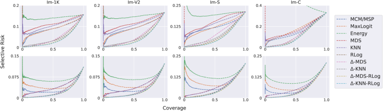
Figure 2: Risk-coverage curves of various selector methods for CLIP (top row) and EVA (bottom row).

We report full selective classification results for CLIP and EVA models in Table 1 and Table 2, respectively. First, let us consider CLIP results. We see that going from MDS and KNN to their NP-informed variants, $\Delta$-MDS and $\Delta$-KNN, leads to roughly $50\%$ reduction in average AURC and NAURC, showing that the assumptions made in the NP-optimality theory hold well in practice. The best average performance is achieved by the linear combinations $\Delta$-KNN-RLog and $\Delta$-MDS-RLog, with $\Delta$-KNN-RLog leading overall in both AURC and NAURC. RLog score ranks third on average, highlighting its strength as a standalone logit-based selector. Motivated by this strong performance, we use RLog in combination with our distance-based scores. Figure 2 (top row) illustrates the risk-coverage curves for selected datasets for CLIP. $\Delta$-KNN-RLog consistently demonstrates the most favorable trade-off across all coverage levels, remaining stable even at low coverage. In contrast, methods such as MDS and Energy suffer from sharp risk increases at low coverage, likely due to the incorrect rejection of samples that contribute disproportionately to risk at low coverage.

For EVA, the ranking is reversed: $\Delta$-MDS-RLog achieves the best overall performance, followed by $\Delta$-KNN-RLog. This supports our hypothesis that MDS-based methods are particularly effective for supervised models due to the close connection between softmax classifiers and Gaussian Discriminant Analysis Lee et al. [2018], which justifies the Gaussian assumptions used in MDS. In contrast, CLIP models trained with contrastive learning Radford et al. [2021] do not satisfy these assumptions, making the nonparametric $\Delta$-KNN combination more suitable. Figure 2 (bottom row) confirms that $\Delta$-MDS-RLog yields the best risk-coverage behavior for supervised learning across all coverage levels. Comparing average NAURC on the full 1K-class datasets, $\Delta$-MDS-RLog with EVA is the top performing selector score, with a slightly better score (0.157) than the best performer on CLIP (0.163).

For practitioners aiming to identify the best overall selective classification setup that considers both the base classifier and the selector, a practical approach is to compare performance using the AURC metric. On the 1K-class datasets, EVA paired with $\Delta$-MDS-RLog achieves an AURC of 3.86, outperforming the DFN CLIP model with $\Delta$-KNN-RLog at 5.01. Despite similar NAURC values, EVA’s higher Im-1K base accuracy ($84.33\%$ vs. DFN CLIP’s $80.39\%$) makes it the preferred choice when considering both components. Intuitively, the optimal setup involves pairing the best selector (here, $\Delta$-MDS-RLog) with the most accurate base classifier.

5.2 Language Experiments

Table 3: Results on Amazon Reviews dataset and its covariate shifted test set at full coverage using DistilBERT trained with LISA.

	In-D		Cov Shift
Method	A	N	A	N
MSP	12.2	0.368	13.9	0.401
MaxLogit	12.6	0.384	14.3	0.416
Energy	12.89	0.397	14.6	0.428
MDS	20.6	0.739	22.2	0.750
KNN	19.4	0.686	21.3	0.711
RLog	12.4	0.376	14.1	0.410
$\Delta$-MDS	12.7	0.389	14.4	0.422
$\Delta$-KNN	12.4	0.374	14.2	0.412
$\Delta$-MDS-RLog	12.2	0.368	13.9	0.401
$\Delta$-KNN-RLog	12.0	0.358	13.8	0.394
$\Delta$-MDS-MSP	11.9	0.354	13.6	0.387
$\Delta$-KNN-MSP	12.0	0.359	13.8	0.396

Table 3 presents results on the Amazon Reviews dataset. Unlike the vision tasks, the best-performing method is $\Delta$-MDS-MSP, followed closely by $\Delta$-MDS-RLog and $\Delta$-KNN-MSP. Since LISA [Yao et al., 2022] uses a softmax classification objective, the superiority of MDS-based selectors supports our hypothesis about their suitability for supervised models. Interestingly, MSP outperforms RLog in this domain, resulting in better performance when combined with $\Delta$-MDS. This highlights another important practical insight that the best linear combination often involves pairing the top-performing standalone distance-based and logit-based score.

5.3 Ablations

Table 4: Ablations experiments on DFN CLIP.

	Im-1K		Im-R		Im-A		ON		Im-V2		Im-S		Im-C		Avg (1K)		Avg (all)
Method	A	N	A	N	A	N	A	N	A	N	A	N	A	N	A	N	A	N
Ablations on $\Delta$-KNN
$\Delta$-KNN no avg	4.66	0.234	1.40	0.234	2.16	0.167	8.87	0.268	5.11	0.239	7.63	0.276	12.4	0.216	7.45	0.241	6.03	0.233
$\Delta$-KNN w/ avg	4.60	0.230	1.42	0.237	1.99	0.149	8.52	0.252	4.99	0.231	7.55	0.272	12.1	0.207	7.32	0.235	5.89	0.225
Ablations on linear combinations
$\Delta$-MDS-$\Delta$-KNN	4.68	0.235	1.98	0.237	2.26	0.149	9.06	0.252	5.11	0.231	7.90	0.272	12.2	0.207	7.46	0.235	6.16	0.225
MSP-RLog	4.82	0.245	0.800	0.120	1.56	0.105	7.51	0.204	5.26	0.249	6.81	0.232	12.5	0.222	7.35	0.237	5.61	0.197
$\Delta$-KNN-MSP	4.57	0.228	1.22	0.199	1.82	0.131	7.58	0.207	4.94	0.228	7.40	0.264	11.8	0.210	7.18	0.244	5.62	0.253
$\Delta$-KNN-RLog	3.98	0.187	0.770	0.115	1.49	0.093	7.14	0.186	4.36	0.190	6.13	0.196	11.3	0.175	6.43	0.187	5.01	0.163

Table 4 summarizes several ablation experiments. First, we justify averaging the top-$k$ nearest neighbor distances in $\Delta$-KNN rather than using the $k$-th distance alone. This modification yields measurable gains, where average AURC improves from 6.03 to 5.89 and NAURC improves from 0.233 to 0.225. We also investigate various combinations of selector scores. For CLIP, $\Delta$-KNN-RLog remains the best across all configurations, outperforming both double-distance combinations (e.g., $\Delta$-MDS-$\Delta$-KNN) and double-logit combinations (e.g., MSP-RLog). Notably, pairing $\Delta$-KNN with RLog significantly outperforms pairing it with MSP, further validating RLog’s role as a strong logit-based complement.

6 Conclusion

We presented a principled framework for designing selector functions for selective classification, grounded in the Neyman–Pearson lemma. This perspective reveals that the optimal selection score is a monotonic transformation of a likelihood ratio, which is a unifying insight that explains the behavior of several existing methods. Building on this foundation, we proposed two novel distance-based scores and their linear combinations with logit-based baselines. Extensive experiments across vision and language tasks under covariate shift demonstrate that our methods achieve state-of-the-art performance across diverse settings.

Limitations and Future Work.

While our focus has been on classification, the Neyman–Pearson framework is general and broadly applicable to other predictive tasks. Exploring selective prediction in settings where uncertainty plays a critical role, such as regression, semantic segmentation, or time series forecasting, presents promising future directions. Additionally, extending these ideas to generative models is especially timely. Large language models (LLMs), for instance, are prone to hallucinations Huang et al. [2025], where the model confidently generates incorrect information. Enabling LLMs to recognize uncertainty and selectively abstain from answering, in other words selective generation, offers another exciting avenue for future work.

7 Acknowledgements

This research is supported by A*STAR under its National Robotics Programme (NRP) (Award M23NBK0053).

Appendix for “Know When to Abstain: Optimal Selective Classification with Likelihood Ratios”

Appendix A Proofs

See 1

Proof.

Recall that we denote $l^{(1)},\cdots,l^{(K)}$ to be the raw logits predicted by a classifier for a given sample ${\bm{x}}$ sorted in descending order and $d^{(1)},\cdots,d^{(K)}$ their values after softmax, then $s_{\text{MSP}}({\bm{x}})=d^{(1)}$ and $s_{\text{RLog}}({\bm{x}})=l^{(1)}-l^{(2)}$.

MSP Optimality.

We begin the proof with showing optimality for MSP. By definition of a calibrated model,

$$p_{c}({\bm{x}}) =\max_{k}p_{\theta}(y=k|{\bm{x}})=d^{(1)}=s_{\text{MSP}}({\bm{x}})$$

$$p_{w}({\bm{x}}) =1-s_{\text{MSP}}({\bm{x}}).$$

We can see that

$$s_{\text{MSP}}({\bm{x}})=\frac{p_{c}({\bm{x}})/p_{w}({\bm{x}})}{1+p_{c}({\bm{x}})/p_{w}({\bm{x}})}.$$ (8)

Note that $s_{\text{MSP}}\in[0,1)$ while $p_{c}({\bm{x}})/p_{w}({\bm{x}})\in[0,\infty)$. The mapping

$$h:[0,\infty)\rightarrow[0,1),\ \ \ h(z)=\frac{z}{1+z}$$

is strictly monotone increasing. This can be seen by looking at the first derivative

$$h^{\prime}(z)=\frac{1}{(1+z)^{2}}>0\ \ \forall z\in[0,\infty).$$

Since it is positive everywhere in the domain, $h$ is strictly increasing on $[0,\infty)$. Thus we have shown that MSP is a monotone transform of the likelihood ratio $p_{c}/p_{w}$, and Corollary 1 tells us that it is Neyman–Pearson optimal.

RLog Optimality.

Next, we prove optimality of RLog. The RLog score can be expressed as the logarithm of the ratio of the top two softmax values:

$$\frac{d^{(1)}}{d^{(2)}}=\frac{e^{l^{(1)}}}{e^{l^{(2)}}}=e^{l^{(1)}-l^{(2)}}=e^{s_{\text{RLog}}({\bm{x}})}$$

thus $s_{\text{RLog}}({\bm{x}})=\log\frac{d^{(1)}}{d^{(2)}}$. We want to connect this to $\log\frac{p_{c}({\bm{x}})}{p_{w}({\bm{x}})}=\log\frac{d^{(1)}}{1-d^{(1)}}$ where we assume a calibrated classifier. Observe that

$$\frac{d^{(1)}}{d^{{(2)}}}=\frac{d^{(1)}}{1-d^{{(1)}}}\times\frac{1-d^{{(1)}}}{d^{{(2)}}}=\frac{d^{(1)}}{1-d^{(1)}}\left(1+\frac{L}{d^{(2)}}\right)$$ (9)

where $L=1-d^{(1)}-d^{(2)}\geq 0$. In the binary classification case $L=0$, thus $s_{\text{RLog}}({\bm{x}})=\log\frac{p_{c}({\bm{x}})}{p_{w}({\bm{x}})}$ exactly. In the multiclass case, the $1+L/d^{(2)}$ factor varies across samples and may alter the ordering of scores. If we assume that most of the probability mass is in the top logits as stated in the theorem, which is empirically supported by high top-5 classification accuracies in prior works Liu et al. [2021], Brock et al. [2021], then $L\approx 0$ and $s_{\text{RLog}}({\bm{x}})\approx\log\frac{p_{c}({\bm{x}})}{p_{w}({\bm{x}})}$. Since logarithm is strictly monotonically increasing, RLog is Neyman–Pearson optimal by Corollary 1. ∎

See 2

Proof.

The likelihood of a multivariate Gaussian in $\mathbb{R}^{d}$ is $p(z;\mu,\Sigma)=(2\pi)^{d/2}\det(\Sigma)^{-1/2}\exp\left(-\frac{1}{2}(x-\mu)^{\top}\Sigma^{-1}(x-\mu)\right)$.

We see that the Mahalanobis distance $D(z;\mu,\Sigma)$ is proportional to the log-likelihood of the multivariate Gaussian. As such, assuming that the underlying $p_{c}$ and $p_{w}$ follow multivariate Gaussians of the form $\mathcal{N}(\mu_{i}^{c},\Sigma^{c})$ and $\mathcal{N}(\mu_{i}^{w},\Sigma^{w})$ respectively,

$$s_{\Delta\text{-MDS}}({\bm{x}}) =D_{\text{MDS}}({\bm{x}};\mu_{i}^{c},\Sigma^{c})-D_{\text{MDS}}({\bm{x}};\mu_{i}^{w},\Sigma^{w})$$

$$=2\log\frac{p_{c}({\bm{z}};\mu_{i}^{c},\Sigma^{c})}{p_{w}({\bm{z}};\mu_{i}^{w},\Sigma^{w})}+\log\frac{\det\Sigma^{c}}{\det\Sigma^{w}}.$$

Therefore, $s_{\Delta\text{-MDS}}({\bm{x}})$ is a monotone transform of $p_{c}/p_{w}$ and is Neyman–Pearson optimal by Corollary 1.

∎

See 3

Proof.

The empirical likelihood of the KNN density estimator Silverman [2018], Zhao and Lai [2022] is given by

$$\hat{p}_{c}({\bm{z}})=\frac{k}{N_{c}V_{d}(u_{k}({\bm{z}}))^{d}},\ \ \ \hat{p}_{w}({\bm{z}})=\frac{k}{N_{w}V_{d}(v_{k}({\bm{z}}))^{d}},$$ (10)

where $k\geq 2$, $u_{k}({\bm{z}})$ and $v_{k}({\bm{z}})$ are the Euclidean distances from ${\bm{z}}$ to its $k$-th nearest neighbor from $A_{c}$ and $A_{w}$ and $V_{d}$ is the unit-ball volume in $\mathbb{R}^{d}$. A classic result of non-parametric nearest neighbor density estimation Loftsgaarden and Quesenberry [1965] states that as $k\rightarrow\infty$ but $k/N_{c}\rightarrow 0$, $k/N_{w}\rightarrow 0$, then $\hat{p}_{c}({\bm{z}})\rightarrow p_{c}({\bm{z}})$ and $\hat{p}_{w}({\bm{z}})\rightarrow p_{w}({\bm{z}})$ for every ${\bm{z}}$. In other words, the empirical KNN density estimator converges to the true density under the stated asymptotic conditions.

One can see that the difference in log-likelihoods is

$$\log\hat{p}_{c}({\bm{z}})-\log\hat{p}_{w}({\bm{z}})=-d\log u_{k}({\bm{z}})+d\log v_{k}({\bm{z}})+\log\frac{N_{w}}{N_{c}}.$$ (11)

Therefore

$$s_{\Delta\text{-KNN}}({\bm{z}})\triangleq-\log u_{k}({\bm{z}})+\log v_{k}({\bm{z}})=\frac{1}{d}\log\frac{\hat{p}_{c}({\bm{z}})}{\hat{p}_{w}({\bm{z}})}-\frac{1}{d}\log\frac{N_{w}}{N_{c}}.$$ (12)

Since the last term is constant, $s_{\Delta\text{-KNN}}({\bm{z}})$ is a monotone transform of $\frac{\hat{p}_{c}({\bm{z}})}{\hat{p}_{w}({\bm{z}})}$. Under the stated conditions on $k,N_{c}$ and $N_{w}$, the empirical likelihoods converge to the true likelihoods $p_{c}$ and $p_{w}$, thus $s_{\Delta\text{-KNN}}({\bm{z}})$ is also Neyman–Pearson optimal. ∎

See 2

Proof.

Let

$$L_{1}({\bm{x}})=\frac{p_{c}^{(1)}({\bm{x}})}{p_{w}^{(1)}({\bm{x}})},\ \ \ L_{2}({\bm{x}})=\frac{p_{c}^{(2)}({\bm{x}})}{p_{w}^{(2)}({\bm{x}})}.$$ (13)

Since each score is already a strictly monotone transform of $L({\bm{x}})$, we are free to re-express the scores in any other convenient monotone scale without affecting relative ordering and thus Neyman–Pearson optimality. Therefore, without loss of generality, we will let $s_{i}({\bm{x}})=\log\frac{p_{c}^{(i)}({\bm{x}})}{p_{w}^{(i)}({\bm{x}})},i=1,2$, which are identical to the original scores in terms of sample acceptance and rejection patterns.

Given $\lambda\in\mathbb{R}$,

$$t({\bm{x}}) =s_{1}({\bm{x}})+\lambda s_{2}({\bm{x}})$$ (14)

$$=\log L_{1}({\bm{x}})+\lambda\log L_{2}({\bm{x}})$$ (15)

$$=\log(L_{2}({\bm{x}})L_{2}({\bm{x}})^{\lambda})$$ (16)

$$=\log\frac{p_{c}^{(1)}(p_{c}^{(2)})^{\lambda}}{p_{w}^{(1)}(p_{w}^{(2)})^{\lambda}}$$ (17)

In other words, $t({\bm{x}})$ is a monotone transform of the tilted likelihood ratio $p_{c}^{(1)}(p_{c}^{(2)})^{\lambda}/p_{w}^{(1)}(p_{w}^{(2)})^{\lambda}$. ∎

When is $t({\bm{x}})$ Neyman–Pearson optimal? Recall $\mathcal{H}_{0}$ and $\mathcal{H}_{1}$ represent the hypotheses that the classifier will make a correct and wrong prediction respectively. If we assume that the density of $\mathcal{H}_{0}$ takes the form of a tilted likelihood $p_{c}^{(1)}(p_{c}^{(2)})^{\lambda}/Z_{c}$, where $Z_{c}$ is a normalizing constant, and vice-versa for $\mathcal{H}_{1}$, then $t({\bm{x}})$ is Neyman–Pearson optimal by Corollary 1.

Appendix B Discussion on Average Top $k$ $\Delta$-KNN Modification

Here we discuss how Neyman–Pearson optimality of the average log-distance formulation of $\Delta$-KNN can hold as described in the main text. Recall that we let $D_{\text{KNN}}({\bm{z}};A_{c})=-\frac{1}{k}\sum_{i=1}^{k}\log(u_{i}({\bm{z}}))$ and vice-versa for $A_{w}$.

For concreteness, let us consider distances to the correct set; the derivation is identical for the wrong set. In the asymptotic limit where $N_{c}$ is large and $k\ll N_{c}$, the ball centered at ${\bm{z}}$ that just encloses its $k$th nearest neighbor (i.e., with volume $V_{d}(u_{k}({\bm{z}}))^{d}$) is so small that the true density is essentially constant over it, so the radii of the first $k$ neighbors are conditionally i.i.d. uniform in the ball.

As such, let us define the normalized variable

$$U_{i}=\left(\frac{u_{i}({\bm{z}})}{u_{k}({\bm{z}})}\right)^{d},\ \ \ i=1,...,k.$$ (18)

Note that $U_{i}\in[0,1]$ for all $i$. Since the joint distribution of $U_{i}$ depends only on $k$, we know from the $i$-th order statistics of $k$ i.i.d. $\mathrm{Uniform}(0,1)$ variables that each $U_{i}$ is Beta-distributed:

$$U_{i}\sim\mathrm{Beta}(i,k-i+1),\ \ \ 0\leq U_{1}\leq\cdots\leq U_{k}=1.$$ (19)

With some algebra, $u_{i}({\bm{z}})=\frac{1}{d}\log U_{i}+\log u_{k}({\bm{z}})$. Then we can show that

$$\frac{1}{k}\sum_{i=1}^{k}\log(u_{i}({\bm{z}}))=\log u_{k}({\bm{z}})+\frac{1}{kd}\sum_{i=1}^{k}\log U_{i}$$ (20)

The second term converges almost surely to

$$\frac{1}{kd}\sum_{i=1}^{k}\log U_{i}\to\frac{1}{d}\int_{0}^{1}\log x\ \mathrm{d}x=-\frac{1}{d}$$ (21)

as $k\to\infty$ as it is a sum of $k$ i.i.d. $\mathrm{Uniform}(0,1)$ random variables.

In other words, in the asymptotic limit the average log-distance is a monotone transform of the log-distance itself. By substituting Eq. 20 back into Eq. 11 for distances to both correct and wrong sets, we see that the modified $\Delta$-KNN formulation is still a monotone transform of the likelihood ratio $p_{c}/p_{w}$, thus suggesting Neyman-Pearson optimality under Corollary 1.

Appendix C Algorithm Pseudocode for Proposed Scores

Algorithm 1 Scoring with $\Delta$-MDS and its linear combination

1:Trained classifier $f$, feature extractor $\phi$ (typically penultimate or final layer of $f$), training set $\mathcal{D}_{\text{train}}=\{({\bm{x}}_{i},y_{i})\}$, test set $\mathcal{D}_{\text{test}}=\{{\bm{x}}_{j}\}$, optional logit-based score function $s_{\text{logit}}({\bm{x}})$, combination weight $\lambda$

2:Selector scores $s({\bm{x}})$ for each ${\bm{x}}\in\mathcal{D}_{\text{test}}$

3:Initialize $\mathcal{A}_{c}^{(i)}\leftarrow\emptyset$ and $\mathcal{A}_{w}^{(i)}\leftarrow\emptyset$ for $i=1$ to $K$ $\triangleright$ Class-wise correct and incorrect feature sets

4:for each $({\bm{x}},y)$ in $\mathcal{D}_{\text{train}}$ do

5:  $\hat{y}\leftarrow f({\bm{x}})$

6:  ${\bm{z}}\leftarrow\phi({\bm{x}})$

7:  if $\hat{y}=y$ then

8:    Add ${\bm{z}}$ to $\mathcal{A}_{c}^{(y)}$

9:  else

10:    Add ${\bm{z}}$ to $\mathcal{A}_{w}^{(y)}$

11:  end if

12:end for

13:Compute $\{\mu_{i}^{c},\Sigma^{c}\}_{i=1}^{K}$ and $\{\mu_{i}^{w},\Sigma^{w}\}_{i=1}^{K}$ from $\mathcal{A}_{c}$ and $\mathcal{A}_{w}$

14:for each ${\bm{x}}$ in $\mathcal{D}_{\text{test}}$ do

15:  ${\bm{z}}\leftarrow\phi({\bm{x}})$

16:  $d_{c}\leftarrow\max_{i}-({\bm{z}}-\mu_{i}^{c})^{\top}(\Sigma^{c})^{-1}({\bm{z}}-\mu_{i}^{c})$

17:  $d_{w}\leftarrow\max_{i}-({\bm{z}}-\mu_{i}^{w})^{\top}(\Sigma^{w})^{-1}({\bm{z}}-\mu_{i}^{w})$

18:  $s_{\Delta\text{-MDS}}({\bm{x}})\leftarrow d_{c}-d_{w}$

19:  if using linear combination then

20:    $s({\bm{x}})\leftarrow s_{\Delta\text{-MDS}}({\bm{x}})+\lambda\cdot s_{\text{logit}}({\bm{x}})$

21:  else

22:    $s({\bm{x}})\leftarrow s_{\Delta\text{-MDS}}({\bm{x}})$

23:  end if

24:end for

25:return $\{s({\bm{x}})\}$ for each ${\bm{x}}\in\mathcal{D}_{\text{test}}$

Algorithm 2 Scoring with $\Delta$-KNN and its linear combination

1:Trained classifier $f$, feature extractor $\phi$ (typically penultimate or final layer of $f$), training set $\mathcal{D}_{\text{train}}=\{({\bm{x}}_{i},y_{i})\}$, test set $\mathcal{D}_{\text{test}}=\{{\bm{x}}_{j}\}$, number of neighbors $k$, optional logit-based score function $s_{\text{logit}}({\bm{x}})$, combination weight $\lambda$

2:Selector scores $s({\bm{x}})$ for each ${\bm{x}}\in\mathcal{D}_{\text{test}}$

3:Initialize $\mathcal{A}_{c}\leftarrow\emptyset$, $\mathcal{A}_{w}\leftarrow\emptyset$ $\triangleright$ Global sets of correct and incorrect features

4:for each $({\bm{x}},y)$ in $\mathcal{D}_{\text{train}}$ do

5:  $\hat{y}\leftarrow f({\bm{x}})$

6:  ${\bm{z}}\leftarrow\phi({\bm{x}})$

7:  if $\hat{y}=y$ then

8:    Add ${\bm{z}}$ to $\mathcal{A}_{c}$

9:  else

10:    Add ${\bm{z}}$ to $\mathcal{A}_{w}$

11:  end if

12:end for

13:for each ${\bm{x}}$ in $\mathcal{D}_{\text{test}}$ do

14:  ${\bm{z}}\leftarrow\phi({\bm{x}})$

15:  Compute $\{u_{i}\}_{i=1}^{k}\leftarrow$ distances from ${\bm{z}}$ to $k$ nearest neighbors in $\mathcal{A}_{c}$

16:  Compute $\{v_{i}\}_{i=1}^{k}\leftarrow$ distances from ${\bm{z}}$ to $k$ nearest neighbors in $\mathcal{A}_{w}$

17:  $d_{c}\leftarrow-\frac{1}{k}\sum_{i=1}^{k}\log(u_{i})$

18:  $d_{w}\leftarrow-\frac{1}{k}\sum_{i=1}^{k}\log(v_{i})$

19:  $s_{\Delta\text{-KNN}}({\bm{x}})\leftarrow d_{c}-d_{w}$

20:  if using linear combination then

21:    $s({\bm{x}})\leftarrow s_{\Delta\text{-KNN}}({\bm{x}})+\lambda\cdot s_{\text{logit}}({\bm{x}})$

22:  else

23:    $s({\bm{x}})\leftarrow s_{\Delta\text{-KNN}}({\bm{x}})$

24:  end if

25:end for

26:return $\{s({\bm{x}})\}$ for each ${\bm{x}}\in\mathcal{D}_{\text{test}}$

Appendix D Experimental Details

Table 5: Values of $\lambda$ and $k$ for results reported in Sec. 5.

Method	$\lambda$	$k$
DFN CLIP
KNN	-	50
$\Delta$-KNN	-	25
$\Delta$-MDS-RLog	10000	-
$\Delta$-KNN-RLog	10	25
Eva
KNN	-	50
$\Delta$-KNN	-	25
$\Delta$-MDS-RLog	1000	-
$\Delta$-KNN-RLog	0.5	25
DistilBERT
KNN	-	50
$\Delta$-KNN	-	25
$\Delta$-MDS-RLog	1000	-
$\Delta$-KNN-RLog	0.05	25
$\Delta$-MDS-MSP	1000	-
$\Delta$-KNN-MSP	0.5	25

Image Experiments.

This section outlines the models and datasets used in the vision experiments in Section 5.1. For classifiers, we use the ViT-H/14 variant for DFN CLIP and the “Giant” variant of EVA, both with patch size 14. Pretrained weights are obtained from the OpenCLIP Cherti et al. [2023] and timm libraries, respectively.

ImageNet and its covariate-shifted variants are downloaded from their respective open-source repositories. For ImageNetV2, we use the MatchedFrequency test set to match the frequency distribution of the original ImageNet. For ImageNet-C, we evaluate using corruption level 5 to simulate the most challenging conditions. The dataset includes four corruption categories: 1) blur, 2) digital, 3) noise, and 4) weather. Each category contains multiple corruption types (e.g., Gaussian, impulse, and shot noise under the noise category). To ensure balanced evaluation, we first average results within each category, then average across the four categories to give equal weight to each corruption type.

For logit-based scores with CLIP, we are required to construct logits over class concepts by taking the dot product between the text embedding $T_{\theta}({\bm{c}})$ of class concepts ${\bm{c}}$ and the image embedding, $\phi({\bm{x}})$, where $T_{\theta}$ is the text encoder of CLIP. Given a class label $y$, we construct the class concept with the template “a real, high-quality, clear and clean photo of a {$y$}” when computing the confidence scores for logit-based selectors. We found this to improve scores slightly as opposed to using the default template in the original work Radford et al. [2021]. We attribute this to the hypothesis that CLIP should produce lower confidence scores when faced with covariate-shifted inputs, such as sketches or corrupted images, as the error rate on covariate shifts are much higher Heng and Soh [2025] than on Im-1K, which are generally clear and well-lit photographs.

Distance-based methods such as MDS, KNN, and our proposed variants compute distances in the feature space. For CLIP, we use the output of the final layer of the vision encoder; for EVA, we use the penultimate layer output.

The hyperparameters $\lambda$ (for linear combinations) and $k$ (for KNN-based scores) used in the experiments reported in Table 1 and Table 2 are summarized in Table 5. All experiments are conducted on a single NVIDIA A6000 GPU with 48GB of memory.

Language Experiments.

For language experiments, we fine-tune a DistilBERT model on the Amazon Reviews dataset using the training pipeline provided in the official LISA repository, with default hyperparameters. For distance-based selectors, we extract features from the penultimate layer of DistilBERT, consistent with the EVA setting. The values of $\lambda$ and $k$ used in Table 3 are also listed in Table 5. All language experiments are run on a single NVIDIA A6000 48GB GPU.

References

- Geifman and El-Yaniv [2017] Yonatan Geifman and Ran El-Yaniv. Selective classification for deep neural networks. Advances in neural information processing systems, 30, 2017.
- Hendrycks and Gimpel [2017] Dan Hendrycks and Kevin Gimpel. A baseline for detecting misclassified and out-of-distribution examples in neural networks. In International Conference on Learning Representations, 2017. URL https://openreview.net/forum?id=Hkg4TI9xl.
- Liang et al. [2024] Hengyue Liang, Le Peng, and Ju Sun. Selective classification under distribution shifts. Transactions on Machine Learning Research, 2024. ISSN 2835-8856. URL https://openreview.net/forum?id=dmxMGW6J7N.
- Gal and Ghahramani [2016] Yarin Gal and Zoubin Ghahramani. Dropout as a bayesian approximation: Representing model uncertainty in deep learning. In international conference on machine learning, pages 1050–1059. PMLR, 2016.
- Lee et al. [2018] Kimin Lee, Kibok Lee, Honglak Lee, and Jinwoo Shin. A simple unified framework for detecting out-of-distribution samples and adversarial attacks. Advances in neural information processing systems, 31, 2018.
- Sun et al. [2022] Yiyou Sun, Yifei Ming, Xiaojin Zhu, and Yixuan Li. Out-of-distribution detection with deep nearest neighbors. In International Conference on Machine Learning, pages 20827–20840. PMLR, 2022.
- Geifman and El-Yaniv [2019] Yonatan Geifman and Ran El-Yaniv. Selectivenet: A deep neural network with an integrated reject option. In International conference on machine learning, pages 2151–2159. PMLR, 2019.
- Liu et al. [2019] Ziyin Liu, Zhikang Wang, Paul Pu Liang, Russ R Salakhutdinov, Louis-Philippe Morency, and Masahito Ueda. Deep gamblers: Learning to abstain with portfolio theory. Advances in Neural Information Processing Systems, 32, 2019.
- Huang et al. [2020] Lang Huang, Chao Zhang, and Hongyang Zhang. Self-adaptive training: beyond empirical risk minimization. Advances in neural information processing systems, 33:19365–19376, 2020.
- Chow [1970] C Chow. On optimum recognition error and reject tradeoff. IEEE Transactions on information theory, 16(1):41–46, 1970.
- Heng and Soh [2025] Alvin Heng and Harold Soh. Detecting covariate shifts with vision-language foundation models. In ICLR 2025 Workshop on Foundation Models in the Wild, 2025. URL https://openreview.net/forum?id=SOHJFKH8oc.
- Ming et al. [2022] Yifei Ming, Ziyang Cai, Jiuxiang Gu, Yiyou Sun, Wei Li, and Yixuan Li. Delving into out-of-distribution detection with vision-language representations. Advances in neural information processing systems, 35:35087–35102, 2022.
- Heng et al. [2024] Alvin Heng, Harold Soh, et al. Out-of-distribution detection with a single unconditional diffusion model. Advances in Neural Information Processing Systems, 37:43952–43974, 2024.
- Neyman and Pearson [1933] Jerzy Neyman and Egon Sharpe Pearson. Ix. on the problem of the most efficient tests of statistical hypotheses. Philosophical Transactions of the Royal Society of London. Series A, Containing Papers of a Mathematical or Physical Character, 231(694-706):289–337, 1933.
- Lehmann et al. [1986] Erich Leo Lehmann, Joseph P Romano, et al. Testing statistical hypotheses, volume 3. Springer, 1986.
- Guo et al. [2017] Chuan Guo, Geoff Pleiss, Yu Sun, and Kilian Q Weinberger. On calibration of modern neural networks. In International conference on machine learning, pages 1321–1330. PMLR, 2017.
- Cattelan and Silva [2023] Luís Felipe P Cattelan and Danilo Silva. How to fix a broken confidence estimator: Evaluating post-hoc methods for selective classification with deep neural networks. arXiv preprint arXiv:2305.15508, 2023.
- Fisch et al. [2022] Adam Fisch, Tommi S. Jaakkola, and Regina Barzilay. Calibrated selective classification. Transactions on Machine Learning Research, 2022. ISSN 2835-8856. URL https://openreview.net/forum?id=zFhNBs8GaV.
- Fumera and Roli [2002] Giorgio Fumera and Fabio Roli. Support vector machines with embedded reject option. In Pattern Recognition with Support Vector Machines: First International Workshop, SVM 2002 Niagara Falls, Canada, August 10, 2002 Proceedings, pages 68–82. Springer, 2002.
- Bartlett and Wegkamp [2008] Peter L Bartlett and Marten H Wegkamp. Classification with a reject option using a hinge loss. Journal of Machine Learning Research, 9(8), 2008.
- Hellman [1970] Martin E Hellman. The nearest neighbor classification rule with a reject option. IEEE Transactions on Systems Science and Cybernetics, 6(3):179–185, 1970.
- LeCun et al. [1989] Yann LeCun, Bernhard Boser, John Denker, Donnie Henderson, Richard Howard, Wayne Hubbard, and Lawrence Jackel. Handwritten digit recognition with a back-propagation network. Advances in neural information processing systems, 2, 1989.
- El-Yaniv et al. [2010] Ran El-Yaniv et al. On the foundations of noise-free selective classification. Journal of Machine Learning Research, 11(5), 2010.
- Hendrycks et al. [2019] Dan Hendrycks, Steven Basart, Mantas Mazeika, Andy Zou, Joe Kwon, Mohammadreza Mostajabi, Jacob Steinhardt, and Dawn Song. Scaling out-of-distribution detection for real-world settings. arXiv preprint arXiv:1911.11132, 2019.
- Liu et al. [2020] Weitang Liu, Xiaoyun Wang, John Owens, and Yixuan Li. Energy-based out-of-distribution detection. Advances in neural information processing systems, 33:21464–21475, 2020.
- Galil et al. [2023] Ido Galil, Mohammed Dabbah, and Ran El-Yaniv. What can we learn from the selective prediction and uncertainty estimation performance of 523 imagenet classifiers? In The Eleventh International Conference on Learning Representations, 2023. URL https://openreview.net/forum?id=p66AzKi6Xim.
- Vovk et al. [2005] Vladimir Vovk, Alexander Gammerman, and Glenn Shafer. Algorithmic learning in a random world, volume 29. Springer, 2005.
- Angelopoulos and Bates [2021] Anastasios N Angelopoulos and Stephen Bates. A gentle introduction to conformal prediction and distribution-free uncertainty quantification. arXiv preprint arXiv:2107.07511, 2021.
- Bates et al. [2021] Stephen Bates, Anastasios Angelopoulos, Lihua Lei, Jitendra Malik, and Michael Jordan. Distribution-free, risk-controlling prediction sets. Journal of the ACM (JACM), 68(6):1–34, 2021.
- Angelopoulos et al. [2024] Anastasios Nikolas Angelopoulos, Stephen Bates, Adam Fisch, Lihua Lei, and Tal Schuster. Conformal risk control. In The Twelfth International Conference on Learning Representations, 2024. URL https://openreview.net/forum?id=33XGfHLtZg.
- Hendrycks et al. [2020] Dan Hendrycks, Steven Basart, Norman Mu, Saurav Kadavath, Frank Wang, Evan Dorundo, Rahul Desai, Tyler Lixuan Zhu, Samyak Parajuli, Mike Guo, et al. The many faces of robustness: A critical analysis of out-of-distribution generalization. 2021 ieee. In CVF International Conference on Computer Vision (ICCV), volume 2, 2020.
- Hendrycks et al. [2021] Dan Hendrycks, Kevin Zhao, Steven Basart, Jacob Steinhardt, and Dawn Song. Natural adversarial examples. In Proceedings of the IEEE/CVF conference on computer vision and pattern recognition, pages 15262–15271, 2021.
- Barbu et al. [2019] Andrei Barbu, David Mayo, Julian Alverio, William Luo, Christopher Wang, Dan Gutfreund, Josh Tenenbaum, and Boris Katz. Objectnet: A large-scale bias-controlled dataset for pushing the limits of object recognition models. Advances in neural information processing systems, 32, 2019.
- Recht et al. [2019] Benjamin Recht, Rebecca Roelofs, Ludwig Schmidt, and Vaishaal Shankar. Do imagenet classifiers generalize to imagenet? In International conference on machine learning, pages 5389–5400. PMLR, 2019.
- Wang et al. [2019] Haohan Wang, Songwei Ge, Zachary Lipton, and Eric P Xing. Learning robust global representations by penalizing local predictive power. Advances in Neural Information Processing Systems, 32, 2019.
- Hendrycks and Dietterich [2019] Dan Hendrycks and Thomas Dietterich. Benchmarking neural network robustness to common corruptions and perturbations. arXiv preprint arXiv:1903.12261, 2019.
- Ni et al. [2019] Jianmo Ni, Jiacheng Li, and Julian McAuley. Justifying recommendations using distantly-labeled reviews and fine-grained aspects. In Proceedings of the 2019 conference on empirical methods in natural language processing and the 9th international joint conference on natural language processing (EMNLP-IJCNLP), pages 188–197, 2019.
- Koh et al. [2021] Pang Wei Koh, Shiori Sagawa, Henrik Marklund, Sang Michael Xie, Marvin Zhang, Akshay Balsubramani, Weihua Hu, Michihiro Yasunaga, Richard Lanas Phillips, Irena Gao, et al. Wilds: A benchmark of in-the-wild distribution shifts. In International conference on machine learning, pages 5637–5664. PMLR, 2021.
- Radford et al. [2021] Alec Radford, Jong Wook Kim, Chris Hallacy, Aditya Ramesh, Gabriel Goh, Sandhini Agarwal, Girish Sastry, Amanda Askell, Pamela Mishkin, Jack Clark, et al. Learning transferable visual models from natural language supervision. In International conference on machine learning, pages 8748–8763. PmLR, 2021.
- Fang et al. [2024] Alex Fang, Albin Madappally Jose, Amit Jain, Ludwig Schmidt, Alexander T Toshev, and Vaishaal Shankar. Data filtering networks. In The Twelfth International Conference on Learning Representations, 2024. URL https://openreview.net/forum?id=KAk6ngZ09F.
- Fang et al. [2023] Yuxin Fang, Wen Wang, Binhui Xie, Quan Sun, Ledell Wu, Xinggang Wang, Tiejun Huang, Xinlong Wang, and Yue Cao. Eva: Exploring the limits of masked visual representation learning at scale. In Proceedings of the IEEE/CVF conference on computer vision and pattern recognition, pages 19358–19369, 2023.
- Sanh et al. [2019] Victor Sanh, Lysandre Debut, Julien Chaumond, and Thomas Wolf. Distilbert, a distilled version of bert: smaller, faster, cheaper and lighter. arXiv preprint arXiv:1910.01108, 2019.
- Yao et al. [2022] Huaxiu Yao, Yu Wang, Sai Li, Linjun Zhang, Weixin Liang, James Zou, and Chelsea Finn. Improving out-of-distribution robustness via selective augmentation. In International Conference on Machine Learning, pages 25407–25437. PMLR, 2022.
- Huang et al. [2025] Lei Huang, Weijiang Yu, Weitao Ma, Weihong Zhong, Zhangyin Feng, Haotian Wang, Qianglong Chen, Weihua Peng, Xiaocheng Feng, Bing Qin, et al. A survey on hallucination in large language models: Principles, taxonomy, challenges, and open questions. ACM Transactions on Information Systems, 43(2):1–55, 2025.
- Liu et al. [2021] Ze Liu, Yutong Lin, Yue Cao, Han Hu, Yixuan Wei, Zheng Zhang, Stephen Lin, and Baining Guo. Swin transformer: Hierarchical vision transformer using shifted windows. In Proceedings of the IEEE/CVF international conference on computer vision, pages 10012–10022, 2021.
- Brock et al. [2021] Andy Brock, Soham De, Samuel L Smith, and Karen Simonyan. High-performance large-scale image recognition without normalization. In International conference on machine learning, pages 1059–1071. PMLR, 2021.
- Silverman [2018] Bernard W Silverman. Density estimation for statistics and data analysis. Routledge, 2018.
- Zhao and Lai [2022] Puning Zhao and Lifeng Lai. Analysis of knn density estimation. IEEE Transactions on Information Theory, 68(12):7971–7995, 2022.
- Loftsgaarden and Quesenberry [1965] Don O Loftsgaarden and Charles P Quesenberry. A nonparametric estimate of a multivariate density function. The Annals of Mathematical Statistics, 36(3):1049–1051, 1965.
- Cherti et al. [2023] Mehdi Cherti, Romain Beaumont, Ross Wightman, Mitchell Wortsman, Gabriel Ilharco, Cade Gordon, Christoph Schuhmann, Ludwig Schmidt, and Jenia Jitsev. Reproducible scaling laws for contrastive language-image learning. In Proceedings of the IEEE/CVF conference on computer vision and pattern recognition, pages 2818–2829, 2023.