Test of local realism via entangled $\Lambda\bar{\Lambda}$ system

Abstract

The non-locality of quantum correlations is a fundamental feature of quantum theory. The Bell inequality serves as a benchmark for distinguishing between predictions made by quantum theory and local hidden variable theory (LHVT). Recent advancements in photon-entanglement experiments have addressed potential loopholes and have observed significant violations of variants of Bell inequality. However, examples of Bell inequalities violation in high energy physics are scarce. In this study, we utilize $(10.087\pm 0.044)\times 10^{9}$ $J/\psi$ events collected with the BES-III detector at the BEPCII collider, performing non-local correlation tests using the entangled hyperon pairs. The massive-entangled $\Lambda\bar{\Lambda}$ systems are formed and decay through strong and weak interactions, respectively. Through measurements of the angular distribution of $p\bar{p}$ in $J/\psi\to\gamma\eta_{c}$ and subsequent $\eta_{c}\to\Lambda(p\pi^{-})\bar{\Lambda}(\bar{p}\pi^{+})$ cascade decays, a significant violation of LHVT predictions is observed. The exclusion of LHVT is found to be statistically significant at a level exceeding $5.2\sigma$ in the testing of three Bell-like inequalities.

1 Introduction

Of all the fundamental aspects of quantum mechanics (QM), perhaps the most bizarre is the non-local nature of an entangled system consisting of two or more components, whose quantum state cannot be factored into the tensor product of the quantum state of each individual member. “Local” and “locality” mean that an object is influenced only by its surroundings and that any influence cannot travel faster than the speed of light. Consider two observers, Alice and Bob, who are spatially far apart from each other and possess half of an entangled quanta pair. According to QM, a measurement by Alice can instantaneously affect the state of her partner, and vice versa. This entanglement between observers is non-local, superluminal, and seemingly incompatible with Special Relativity. Einstein called this “spooky action at a distance”. In 1935, Einstein, Podolsky, and Rosen devised a thought experiment, known as the EPR paradox [1]. The paradox led EPR to conclude that "the description of reality given by the wave function in QM is not complete” [1], suggesting the existence of an local hidden variable theory (LHVT).

In 1951, Bohm modified the EPR paradox to make it experimentally accessible [2, 3]. In Bohm’s scheme, a pair of entangled spin-1/2 particles in a spin singlet state are used. If Alice measures the spin of her particle to be along the $z$ direction, Bob should find the spin of his along the $-z$ direction. In 1964, Bell developed his own variant of the EPR paradox [4]. Bell assumed that the measurement results of Alice and Bob could be described by two families of variables. The outcomes of their measurements in space-like separation do not affect each other and are mutually independent (local). Under these assumptions, he provided an upper bound for hidden-variable correlation according to the Bell inequality, which QM can violate in specific regions of parameter space. Bell showed that QM is incompatible with LHVT, which was known as the Bell Theorem. The triumph of the Bell inequality lies in transforming the philosophical debates on the completeness of QM into an experimental criterion.

Numerous optical experiments using entangled photons have been conducted to test Bell inequalities [5, 6, 7, 8, 9, 10, 11]. However, most experiments relied on additional assumptions in order to exclude LHVTs, therefore not closing all the so-called loopholes. There are three commonly admitted loopholes [12]. The locality loophole means the separation of Alice and Bob is not space-like. By increasing the distance between them and shortening the interval of successive measurements, the space-like separation requirement can be met, ensuring no physical information is exchanged between Alice and Bob, even by light. The freedom-of-choice loophole addresses whether Alice and Bob can freely and independently decide what to measure. LHVT postulates that measurements can be performed with mutual independence [13]. The third loophole, known as the fair sampling loophole (or detection loophole) [14, 15, 16], can occur when a subset of detected particles violates a Bell inequality while the total group does not. If an experiment only detects this subset and assumes it represents the entire particels, a loophole is exploited. Closing this loophole is possible by detecting the particles with sufficient efficiency, which was realized in optical experiments[11, 17]. Optical experiments designed to test Bell inequalities have made significant progress in closing potential loopholes [15, 16] since the pioneering work [18]. These experiments, both with specific loopholes and without, have produced results that clearly violate the Bell inequalities [5, 6, 7, 8, 9, 10, 11].

Unlike experiments with entangled photons, studies utilizing entangled-massive particles to investigate local realism [9, 19, 20, 21] are uncommon, and these experiments in low energy region often do not address all three loopholes simultaneously. The detection loophole was addressed in the entangled ion experiments [9, 19] with significant results. The entangled states are prepared with specific ion traps, or nuclear reactions. Here, we present an experiment testing realism with entangled $\Lambda\bar{\Lambda}$ particles. It has three eminent features: the first is that the entangled $\Lambda\bar{\Lambda}$ particles are realized over extremely short distances, accompanied by strong and weak interactions in the decays, severing as a spin self-analyzer. The second feature is that the $\Lambda\bar{\Lambda}$ particles is the maximally entangled states [22] produced from the $\eta_{c}$ decays. The third is concerning the locality loophole, which can be addressed by requiring the space-like criteria applied to the decayed $\Lambda\bar{\Lambda}$ particles. Our experiment does not close the detection loophole, since having a fair sampling of the recorded events is assumed. However, it is a widely accepted fundamental assumption in collider physics [23].

Testing LHVT in high energy physics are challenging, and has garnered substantial attention over the past two decades [24, 25, 26, 27, 28, 29, 30, 31, 32, 33, 34, 35, 36, 37]. The proposed experiments can be categorized into two groups, quark flavor entanglement (also known as quasi-spin) experiments [30, 34, 35] and particle spin entanglement experiments [25, 26, 27, 28, 29, 31, 32, 33, 38, 37]. Tornquist proposed to examine the non-locality of quantum mechanical prediction using the spin-entangled $\Lambda\bar{\Lambda}$ system [39]. The decay $\Lambda(\bar{\Lambda})\to p\pi^{-}(\bar{p}\pi^{+})$ can serve as a spin analyzer for inferring the hyperon spins [40]. Specifically, the spins of $\Lambda$ and $\bar{\Lambda}$ in the $\eta_{c}\to\Lambda\bar{\Lambda}$ process are always opposite and possess a total spin of 0, i.e., $|S\rangle=1/\sqrt{2}(|\uparrow\downarrow\rangle-|\downarrow\uparrow\rangle)$, where $\uparrow$ and $\downarrow$ denote the spin projections of $\Lambda(\bar{\Lambda})$. Due to parity violation in hyperon weak decays, the outgoing proton (anti-proton) exhibits a preference to travel along (against) the polarization direction of the hyperon. Alice and Bob arrange to measure the spins of their respective particles at the $\Lambda$ and $\bar{\Lambda}$ decay vertices, with their measurement axes setting aligned along the momentum directions of the proton and antiproton. The correlation function between these measurements can be expressed as [39]:

$$E(\vec{n}_{1},\vec{n}_{2})\equiv\langle S|\sigma\cdot\vec{n}_{1}\sigma\cdot\vec{n}_{2}|S\rangle=-\vec{n}_{1}\cdot\vec{n}_{2}\equiv-\cos\theta_{p\bar{p}},$$ (1)

where the operator $\sigma\cdot\vec{n}_{1}(\sigma\cdot\vec{n}_{2})$ represents the measurement of $\Lambda(\bar{\Lambda})$ spin projection along the guide axis $n_{1}(n_{2})$, which coincides with the proton (antiproton) momentum direction in the $\Lambda$ ($\bar{\Lambda}$) rest frame. This direction is obtained by boosting the proton(antiproton) momentum to the $\Lambda(\bar{\Lambda})$ center-of-mass system. Here $\theta_{p\bar{p}}$ is the opening angle between $\vec{n}_{1}$ and $\vec{n}_{2}$ with their reference frames superimposed. Thus, LHVT can be experimentally tested by measuring the distribution $I(\theta_{p\bar{p}})$ of angles between the momenta of $p$ and $\bar{p}$ [39],

$$I(\theta_{p\bar{p}})=1+\alpha^{2}\cos\theta_{p\bar{p}},$$ (2)

where $\alpha=\alpha_{\Lambda}=0.750\pm 0.009\pm 0.004$ is the asymmetry parameter of the $\Lambda\to p\pi^{-}$ decay, which can be precisely measured in $J/\psi\to\Lambda(p\pi^{-})\bar{\Lambda}(\bar{p}\pi^{+})$  [41, 42]. If a hidden measurement of $\Lambda$ polarization is carried out before its decay, this reduces to $\alpha^{2}=\alpha_{\Lambda}^{2}/3$. When the Bell inequality is applied to the decay $\eta_{c}\to\Lambda\bar{\Lambda}$, one may get a bound [39] as $|E(\vec{n}_{1},\vec{n}_{2})|\leq 1-{2\theta_{p\bar{p}}\over\pi}$. Substituting with $I(\theta_{p\bar{p}})$, we obtain:

$$|I(\theta_{p\bar{p}})-1|\leq\alpha_{\Lambda}^{2}(1-{2\over\pi}\theta_{p\bar{p}}),$$ (3)

which defines the domain satisfying the Bell inequality. If experimental measurement of the angular distribution $\cos\theta_{p\bar{p}}$ lies outside the region allowed by Bell’s inequality, then a violation of Bell inequality is established.

Later, a freedom-of-choice loophole was identified when testing the Bell inequality using $\Lambda\bar{\Lambda}$ spin entanglement produced in $\eta_{c}$ decays [40, 43]. Compared to optical experiments, the decays of $\Lambda$ and $\bar{\Lambda}$ occur spontaneously, rather being artificially controlled by experimenters at will. The assumption of independence in the decay of $\Lambda$ and $\bar{\Lambda}$ particles is utilized during realism testing. Closing this loophole in high-energy experiments is challenging, as suggested in Ref. [30], requiring dedicated devices for active measurements. Although Ref. [23] suggests that measurements of $\Lambda$ and $\bar{\Lambda}$ decays in the detector could serve as an ideal random generator, the freedom-of-choice loophole remains a significant challenge in high-energy experiments. Nevertheless, we could introduce a weak assumption that the sample survived from the free-will choice should have the same distribution as the detected sample. Thus the presence or absence of free-will choice only affects the sensitivity to test realism, but does not alter the acceptance or rejection of realism conclusions in the high luminosity of collider experiment.

It should be noted that in previous scheme the $\Lambda(\bar{\Lambda})$ decay parameter $\alpha_{\Lambda}(\alpha_{\bar{\Lambda}})$ is introduced in the test of Bell inequality, which will bring about a new loophole. In order to overcome the QM dependence, a new inequality, a Clauser-Horne (CH)-type inequality, was developed [25, 44]. For the $\eta_{c}\to\Lambda\bar{\Lambda}$ decay, the CH inequality can be generalized as [25]

$$P(\vec{n}_{a},\vec{n}^{\prime}_{b})-P(\vec{n}_{a},\vec{n}^{\prime}_{d})+P(\vec{n}_{c},\vec{n}^{\prime}_{b})+P(\vec{n}_{c},\vec{n}^{\prime}_{d})-P(\vec{n}_{c})-P(\vec{n}^{\prime}_{b})+{1-\alpha_{\Lambda}^{2}\over 2}\leq(1-\beta_{\Lambda}){\alpha^{2}_{\Lambda}\over 2}.$$ (4)

Here unit vectors $\vec{n}_{a,c}$ and $\vec{n}^{\prime}_{b,d}$ denote the directions of chosen guide axes used to detect proton and antiproton, respectively. This can be viewed as a generalization of polarizer settings in optical experiments. $P(\vec{n},\vec{n}^{\prime})={1\over 4}(1+\alpha_{\Lambda}^{2}\vec{n}\cdot\vec{n}^{\prime})$ represents the probability to detect an event of proton and antiproton at direction $\vec{n}$ and $\vec{n}^{\prime}$ respectively, coinciding with a $\eta_{c}\to\Lambda(p\pi^{-})\bar{\Lambda}(\bar{p}\pi^{+})$ decay. While $P(\vec{n}_{c})=P(\vec{n}^{\prime}_{b})={1\over 2}$ indicates the probability to detect proton or antiproton alone. Just as the CH inequality is tested in optical experiments, these direction settings are used to characterize the polarization of $\Lambda(\bar{\Lambda})$. In the above inequality, $\beta_{\Lambda}=P/E$, is the velocity of $\Lambda$, and $P$ and $E$ are the $\Lambda$ momentum and energy, respectively. The introduction of $\beta_{\Lambda}$ is necessary to account for the requirement of space-like separation, which decreases the upper bound. The nonzero upper bound of the CH inequality is due to the requirement, described below, of excluding any possible classical communication between the $\Lambda$ and $\bar{\Lambda}$. To directly verify the contradiction between locality and QM, one can obtain the CH inequality by substituting the QM predictions into the above equation. Specifically, the CH inequality is given by:

$${\alpha_{\Lambda}^{2}\over 4}(\cos\theta_{ab}-\cos\theta_{ad}+\cos\theta_{cb}+\cos\theta_{cd})-{\alpha_{\Lambda}^{2}\over 2}\leq(1-\beta_{\Lambda}){\alpha^{2}_{\Lambda}\over 2},$$ (5)

where $\theta_{ij}$ are the angles between $\vec{n}_{i}$ and $\vec{n}^{\prime}_{j}$. To highlight the specific region where the violation of the CH inequality occurs, one selects $\theta_{ab}=\theta_{cb}=\theta_{cd}=\theta_{p\bar{p}}$ and $\theta_{ad}=3\theta_{p\bar{p}}$, resulting in the following expression [25]:

$$CH(\theta_{p\bar{p}})\equiv\alpha_{\Lambda}^{2}\left[{3\cos\theta_{p\bar{p}}-\cos(3\theta_{p\bar{p}})\over 4}-{1\over 2}\right]\leq(1-\beta_{\Lambda}){\alpha^{2}_{\Lambda}\over 2}.$$ (6)

Since $\alpha_{\Lambda}^{2}>0$, the above inequality may test the LHVT evidently independent of $\alpha_{\Lambda}$, superior to inequality (3). From the generalized CH inequality, the maximum violation of the inequality, $\alpha_{\Lambda}^{2}({\sqrt{2}\over 2}-{1\over 2})\leq(1-\beta_{\Lambda}){\alpha^{2}_{\Lambda}\over 2}$ with $\beta_{\Lambda}\sim 0.7$, is achieved when $\theta_{p\bar{p}}=\pi/4$. If a significant number of events can be observed near $\theta_{p\bar{p}}=\pi/4$ with $CH(\theta_{p\bar{p}})>(1-\beta_{\Lambda}){\alpha^{2}_{\Lambda}\over 2}$, the prediction of quantum theory is inconsistent with the locality.

2 BESIII EXPERIMENT AND MONTE CARLO SIMULATION

The BESIII detector [45] records symmetric $e^{+}e^{-}$ collisions provided by the BEPCII storage ring [46], which operates with a peak luminosity of 1$\times$10³³ cm^-2s^-1 in the center-of-mass energy range from 2.0 GeV to 4.95 GeV. The cylindrical core of the BESIII detector covers 93% of the full solid angle and consists of a helium-based multilayer drift chamber (MDC), a plastic scintillator time-of-flight system (TOF), and a CsI(Tl) electromagnetic calorimeter (EMC), which are all enclosed in a superconducting solenoidal magnet providing a 1.0 T (0.9 T for 2012 $J/\psi$ data) magnetic field. The tracks of charged particles are reconstructed and their momenta are determined in the MDC, while showers from photons are reconstructed and their energy deposits are measured in the EMC.

Monte Carlo (MC) simulations are used to optimize the event selection criteria and estimate the background sources, as well as to determine the efficiency. geant4 [47] based MC software, including the geometric description of the BESIII detector [48, 49] and its response, is used to simulate the MC samples. The inclusive MC sample includes the production of vector charmonium(-like) states and the continuum processes incorporated in kkmc [50]. All particle decays are modelled with evtgen [51, 52] using the branching fractions either taken from the Particle Data Group [53], or otherwise estimated with lundcharm [54, 55].

3 EVENTS SELECTION

In this work, an experimental test of the non-local correlation in the $\Lambda\bar{\Lambda}$ system is performed using $(10.087\pm 0.044)\times 10^{9}$ $J/\psi$ events collected by the BESIII detector at the BEPCII $e^{+}e^{-}$ collider [56] through $J/\psi\to\gamma\eta_{c}\to\gamma\Lambda(p\pi^{-})\bar{\Lambda}(\bar{p}\pi^{+})$ decays, and the event selection criteria are described in the Appendix below. The locality loophole is closed by applying a requirement on the hyperon decay length to guarantee the spatial separation between their decays. From the $e^{+}e^{-}$ interaction point, where $\eta_{c}$ decays into $\Lambda$ and $\bar{\Lambda}$ instantaneously, the average flight distance of $\Lambda$ ($\bar{\Lambda}$) to the decay point is about 6.95 cm. The $\Lambda$ and $\bar{\Lambda}$ candidates are identified by fitting the secondary vertices to $p\pi^{-}$ and $\bar{p}\pi^{+}$ final states, respectively. The fits yield the decay lengths $L_{1}$ and $L_{2}$, which are the flight distances of the $\Lambda$ and $\bar{\Lambda}$ from the beam interaction point, respectively. Testing LHVT requires space-like separation of $\Lambda$ and $\bar{\Lambda}$, and $L_{1}$ and $L_{2}$ are used to select separated events [39, 25], i.e.

$${1\over S}\leq{L_{1}\over L_{2}}\leq S,\text{~with~}S={1+\beta_{\Lambda}\over 1-\beta_{\Lambda}}.$$ (7)

After applying the above selection criteria, 23,313 events survived. The detection efficiency was determined to be 8.2%. The number of background events was estimated to be 4,319, mainly from the decays of $J/\psi\to\bar{\Lambda}\Sigma^{0}(\gamma\Lambda)+c.c.,~\gamma\bar{\Lambda}\Sigma^{0}(\gamma\Lambda)+c.c.,~\Sigma^{0}(\gamma\Lambda)\bar{\Sigma}^{0}(\gamma\bar{\Lambda}),\text{and}~\pi^{0}(2\gamma)\Lambda\bar{\Lambda}$.

The transverse view of the BESIII detector in Fig. 1 shows an event with $\Lambda\bar{\Lambda}$ space-like separation. The neutral hyperon pair originates from the $\eta_{c}$ decay at the primary vertex. The decay-length ratio is $L_{1}/L_{2}=2.711$ for this event. The $p\bar{p}$ daughter particles fly along curves with large radii, and the $\pi^{\pm}$ along curves with smaller radii. The momenta of the hyperons are calculated from those of their daughter particles, and $S=4.854$ here, satisfying the space-like separation criterion.

\begin{overpic}[width=260.17464pt]{draft_evtdisplay_simpleversion.eps} \end{overpic}

Fig. 1: | Transverse view of a $\Lambda\bar{\Lambda}$ space-like separation event in the detector. The center of the detector corresponds to the $e^{+}e^{-}$ interaction point, where the $J/\psi$ is produced and decays instantaneously into a photon and the $\eta_{c}$ meson. The $\eta_{c}$ itself decays also instantaneously into a hyperon pair $\Lambda\bar{\Lambda}$, and the $\Lambda(\bar{\Lambda})$ decays into the charged particles $p$ and $\pi^{-}$ ($\bar{p}$ and $\pi^{+}$). The trajectories of the charged tracks can be seen as black curves. The areas colored beige, yellow and light blue correspond to the MDC, TOF and EMC of the BESIII detector, respectively.

4 AMPLITUDE ANALYSIS

An amplitude analysis is used to calculate the probability of events with $\gamma\Lambda\bar{\Lambda}$ final states for the selected events, which are divided into three categories. The first category refers to background events in which the final states are misidentified as $\gamma\Lambda\bar{\Lambda}$; the second corresponds to spin-entangelment signal events including the intermediate state $\eta_{c}$ and the non-resonant ($NR$) case with quantum numbers $J^{P}=0^{-}$, denoted by $NR(0^{-})$; the last category is due to spin-entanglement background events, i.e., $J/\psi\to\gamma NR(0^{+},1^{+},2^{+})\to\gamma\Lambda\bar{\Lambda}$ decays. The amplitudes corresponding to $NR(0^{\pm},1^{+},2^{+})$ with $J^{P}$ are denoted by $M^{J^{P}}$, which are obtained by multiplying the helicity amplitudes of all steps of the cascade decay.

An amplitude model is used to isolate the signal events from the $J/\psi$ cascade decay, in which the probability of finding the intermediate state $J^{P}$ is calculated by evaluating the weight factor of the MC event $i$, which is defined as,

$$W_{i}(\vec{\xi},\vec{\omega}_{i})={1\over\mathcal{N}}\overline{\sum}|M^{J^{P}}(\vec{\xi},\vec{\lambda},\vec{\omega}_{i})|^{2}{N_{\text{dt}}-N_{\text{bg}}\over N_{\text{MC}}},$$ (8)

where $\overline{\sum}$ denotes the summation over the helicities of the photon, proton and antiproton, and taking the average over the spin third-component of the J/$\psi$. The variables $N_{\text{dt}}$, $N_{\text{bg}}$ and $N_{\text{MC}}$ denote the numbers of data, background and MC phase-space events, respectively. $\mathcal{N}$ is a normalization factor calculated as the amplitude squared average of $N_{\text{MC}}$ events. The vector $\vec{\lambda}$ denotes the helicities of the particles involved. The parameter $\vec{\xi}$ is determined by fitting the amplitudes to the data events with 9-dimensional vectors $\vec{\omega}_{i}$.

The mass spectra of $\gamma\Lambda/\gamma\bar{\Lambda}$ and $\Lambda\bar{\Lambda}$ can be well described by $NR$ in conjunction with the $\eta_{c}$ signal, and the statistical significance of $\eta_{c}$ is determined to be more than 5$\sigma$. The criterion to include $NR$ is that its statistical significance is more than $5\sigma$, and the spin and parity of these states surviving the event selection criteria are determined to be $J^{P}=0^{\pm},1^{+}$, or $2^{+}$. However, only the $\Lambda\bar{\Lambda}$ pairs produced by the decays of $\eta_{c}$ and $NR(0^{-})$, totaling 14716 observed events, are in the spin entangled state being studied. The contributions from other non-resonant states with $J^{P}=(0^{+},1^{+},2^{+})$ constitute the entanglement background.(More details could be found in the Appendix)

5 RESULT

To test the realism, the distribution of $CH(\theta_{p\bar{p}})$ for the $\Lambda\bar{\Lambda}$ spin-entangled events are measured, where the background and entanglement background are subtracted using simulated events weighted to agree with the amplitude analysis solution. More detail can be found in the Appendix. The distribution of $CH(\theta_{p\bar{p}})/\alpha_{\Lambda}^{2}$ for the $\Lambda\bar{\Lambda}$ spin-entanglement events is shown in Fig.2. The points with total error bars, corresponding to signal, are the numbers of events with simulated background and weighted $NR(0^{+},1^{+},2^{+})$ events subtracted in each bin, corrected by the detection efficiency times the value of $CH(\theta_{p\bar{p}})/\alpha_{\Lambda}^{2}$. For comparison with the theoretical distribution, the points are further scaled by the ratio of the area under the signal $CH(\theta_{p\bar{p}})/\alpha_{\Lambda}^{2}$ distribution divided by that under the theoretical $CH(\theta_{p\bar{p}})/\alpha_{\Lambda}^{2}$ distribution. The events in the shaded region above $\frac{(1-\beta_{\Lambda})}{2}$ line are consistent with the QM prediction [25], and they are located above the upper bound of the LHVT prediction, indicating that the CH inequality is significantly violated. We obtain $\chi^{2}=\sum_{i=1}^{4}(N_{i}-U_{b})^{2}/\sigma_{i}^{2}=30.9$ for the two bins in this interval, where $N_{i}(\sigma_{i})$ denotes the measurement (total uncertainty) of the $i$th bin, and $U_{b}$ is the upper boundary of LHVT [25]. This shows the significance of rejecting the CH inequality is determined to be 5.2$\sigma$.

We also test the Bell and Clauser–Horne–Shimony–Holt (CHSH) inequalities in two QM dependent schemes, with further details provided in the Appendix. To measure the $p\bar{p}$ angular distribution, the significance to exclude the Bell inequality region is determined to be $8.9\sigma$. The measurements are consistent with the QM predictions and clearly contradict the predictions of the LHVT. We check the CHSH inequality by calculating the $C_{ij}$ tensor using a TOY MC method based on amplitude analysis. A $\chi^{2}$ test shows that excluding the LHVT is significant at a level exceeding $10\sigma$.

\begin{overpic}[width=260.17464pt]{ch.eps} \end{overpic}

Fig. 2: | The distribution of $CH(\theta_{p\bar{p}})/\alpha_{\Lambda}^{2}=[\frac{3\cos\theta_{p\bar{p}}-\cos(3\theta_{p\bar{p}})}{4}-\frac{1}{2}]$. The points with total error bars are the measurements, the solid line is the QM prediction, and the dashed line is the upper bound of the LHVT prediction. The shaded area above the dashed line indicates the violation of the $CH(\theta_{p\bar{p}})$ inequality.

Using $(10.087\pm 0.044)\times 10^{9}$ $J/\psi$ events collected with the BESIII experiment, a non-local correlation test for the spin entanglement of a hyperon system in $J/\psi\to\gamma\eta_{c},\eta_{c}\to\Lambda\bar{\Lambda}$ decays is carried out for the first time. The decay lengths of the $\Lambda$ and $\bar{\Lambda}$ particles, detectable at a macroscopic scale, are used to control the selection of space-like separation events, which ensures that the locality loophole is closed. The $CH(\theta_{p\bar{p}})$ angular distributions between the proton and antiproton are in agreement with the QM predictions within their uncertainties. The Bell and CHSH inequalities are also tested, which however are QM dependent. The three tests have significantly excluded LHVT, confirming the existence of non-local quantum correlations, with the significances of $5.2\sigma$, $8.9\sigma$ and larger than $10\sigma$ for the CH, Bell and CHSH inequalities, respectively. These results confirm the existence of quantum entanglement and the violation of the Bell inequality in the presence of strong and weak interactions. It tells that the entanglement emerging from these fundamental interactions also exhibits quantum correlation and nonlocality, which deepens our understanding of the physical reality.

Appendix 1 Event selection

The final state of a candidate event is required to contain four charged tracks ($p,{\bar{p}},\pi^{+}$ and $\pi^{-}$) and at least one good photon ($\gamma$). The charged tracks reconstructed in the MDC are required to satisfy $|\cos\theta|\leq 0.93$, where $\theta$ is defined with respect to the $z$-axis which is the symmetry axis of the MDC. The momentum distributions of protons and pions from the signal process are well separated and do not overlap, as shown in Fig. 3. Therefore, a simple momentum criterion is applied: if the momentum of the particle is larger than 0.4 GeV/$c$, it will be identified as a proton, otherwise it will be identified as a pion. Next, the $\Lambda\to p\pi^{-}$ and $\bar{\Lambda}\to\bar{p}\pi^{+}$ decays are reconstructed, requiring for each that two tracks with opposite charges can be successfully fit to a secondary vertex and requiring the invariant mass of the hyperon lies in the interval of [1.008,1.124] GeV/$c^{2}$. The hyperon decay length distributions of the MC events are in good agreement with the data (shown in Figs. 4).

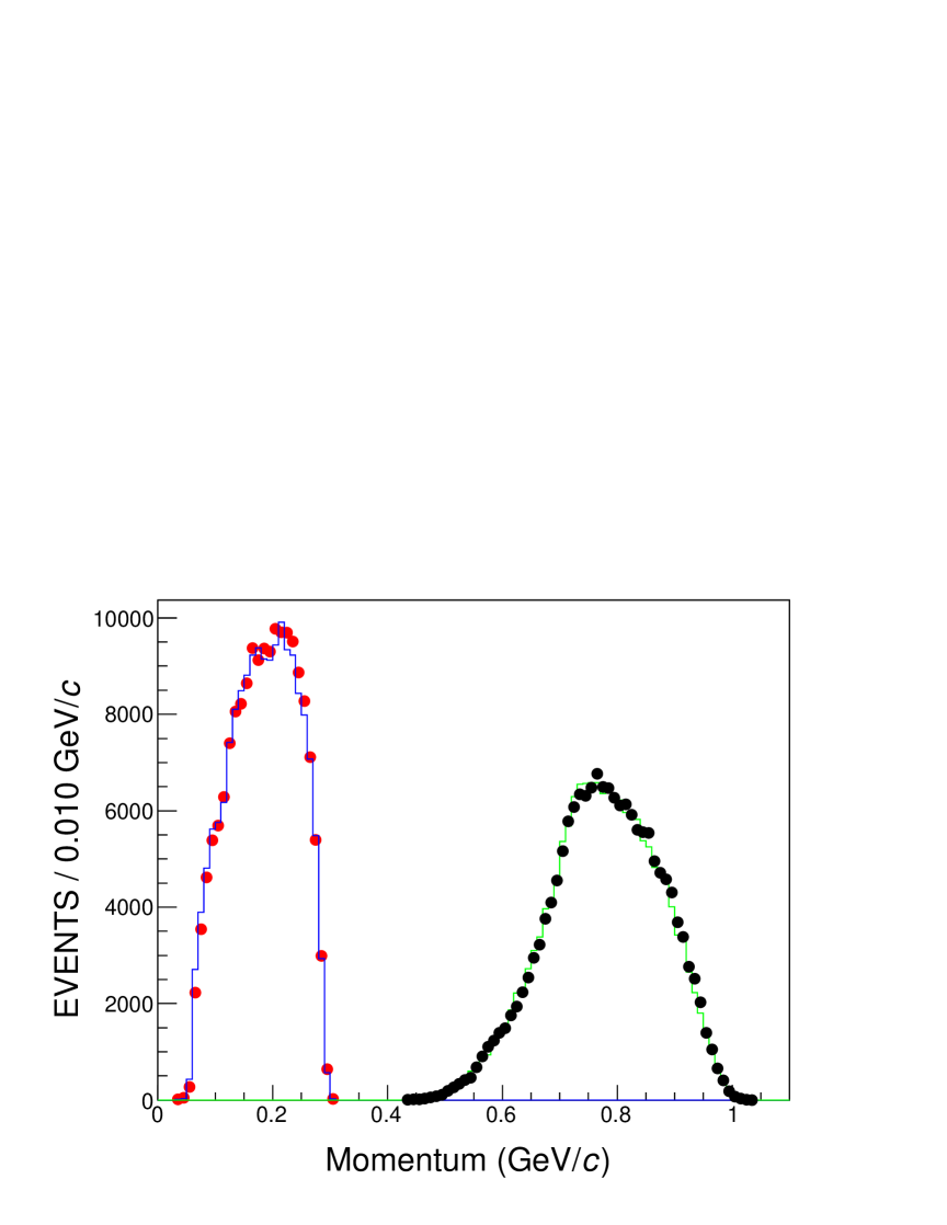
Fig. 3: Comparison of the momentum distributions of pions and protons for the decay $J/\psi\to\gamma\eta_{c}\to\gamma\Lambda\bar{\Lambda}\to\gamma p\pi^{-}\bar{p}\pi^{+}$ with signal MC events. The black dots and green line denote data and MC events, respectively, corresponding to $p$ ($\bar{p}$), and the red dots and blue line denote data and MC events corresponding to $\pi^{+}$ ($\pi^{-}$).

\begin{overpic}[width=346.89731pt]{draft_comp_decleng1_MCData.eps}\put(25.0,60.0){(a)} \end{overpic}

\begin{overpic}[width=346.89731pt]{draft_comp_decleng2_MCData.eps}\put(25.0,60.0){(b)} \end{overpic}

Fig. 4: The comparison of decay lengths of (a) $\Lambda$ and (b) $\bar{\Lambda}$. The red dots denote data, and the black histograms denote the signal MC sample.

Photon candidates are reconstructed from showers in the EMC within 700 ns from the event start time. The deposited energy of each shower is required to be greater than 25 MeV in the barrel region ($|\cos\theta|\leq 0.8$) or 50 MeV in the end cap region ($0.86\leq|\cos\theta|\leq 0.92$), and the minimum opening angle between the shower and the pion or nucleon (antinucleon) is required to be greater than $20^{\circ}(30^{\circ})$. The radiative photon is selected through a four constraint (4C) kinematic fit requiring energy and momentum conservation in the decay $J/\psi\to\gamma\Lambda\bar{\Lambda}$, and events with $\chi^{2}_{\rm 4C}(\gamma\Lambda\bar{\Lambda})<\chi^{2}_{\rm 4C}(\gamma\gamma\Lambda\bar{\Lambda})$ and $\chi_{\rm 4C}^{2}(\gamma\Lambda\bar{\Lambda})<30$ are retained for further analysis, where $\chi_{\rm 4C}^{2}$ is the goodness of fit of the kinematic fit. In order to remove background events containing $J/\psi\to\Sigma^{0}\bar{\Sigma}^{0},\Lambda\bar{\Sigma}^{0}+c.c.$ decays, the invariant mass of $\gamma\Lambda/\gamma\bar{\Lambda}$ is required to satisfy $|M_{\gamma\Lambda/\gamma\bar{\Lambda}}-M_{\Sigma^{0}}|>0.009$ GeV$/c^{2}$, where $M_{\Sigma^{0}}$ is the known mass of $\Sigma^{0}$ [53].

Appendix 2 Amplitude analysis using maximum likelihood fit

The amplitude of the $\eta_{c}$ or non-resonant ($NR$) decays depends on a 9-dimensional vector $\vec{\omega}=(M_{\Lambda\bar{\Lambda}},\theta_{\gamma},\phi_{\gamma},\theta_{\Lambda},\phi_{\Lambda},\theta_{p},\phi_{p},\theta_{\bar{p}},\phi_{\bar{p}})$, where $M_{\Lambda\bar{\Lambda}}$ is the invariant mass of the $\Lambda\bar{\Lambda}$ system and $\theta_{i}$ and $\phi_{i}(i=\gamma,\Lambda,p,\bar{p})$ denote, respectively, the polar and azimuthal angles of particle $i$ in their helicity coordinate systems, which are illustrated in Fig. 5. For the decay $A\to B+C$, the polar angle $\theta$ is defined as the angle between the momentum vectors $\vec{p}_{A}$ and $\vec{p}_{B}$, which are defined in the rest frame of the mother particle. The azimuthal angle $\phi$ is defined as the angle between the production and decay planes of particle $A$.

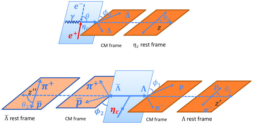
Fig. 5: Illustration of helicity angles defined in each step of a decay chain. Helicity angles in $J/\psi\to\gamma\eta_{c},\eta_{c}\to\Lambda\bar{\Lambda}$ decays, and $\eta_{c}\to\Lambda\bar{\Lambda}\to p\bar{p}\pi^{+}\pi^{-}$ decays

For the cascade decays $J/\psi(m)\to\gamma(\lambda_{\gamma})R(\lambda_{0}),~R\to\Lambda(\lambda_{1})\bar{\Lambda}(\lambda_{2}),~\Lambda\to p(\lambda_{3})\pi^{-}$ and $\bar{\Lambda}\to\bar{p}(\lambda_{4})\pi^{+}$, where $m$ and $\lambda_{i}$ denote the third component of the $J/\psi$ spin and the helicity of the particle $i$, respectively, the amplitudes are expressed as

$$M^{J^{P}}(\vec{\xi},\vec{\lambda},\vec{\omega}) = \sum_{\lambda_{0},\lambda_{1},\lambda_{2}}D^{1*}_{m,\lambda_{\gamma}-\lambda_{0}}(\phi_{\gamma},\theta_{\gamma},0)D^{J*}_{\lambda_{0},\lambda_{1}-\lambda_{2}}(\phi_{\Lambda},\theta_{\Lambda},0)D^{1/2*}_{\lambda_{1},\lambda_{3}}(\phi_{p},\theta_{p},0)D^{1/2*}_{\lambda_{2},\lambda_{4}}(\phi_{\bar{p}},\theta_{\bar{p}},0)$$ (9)

$$\times BW(M_{\Lambda\bar{\Lambda}},M_{0},\Gamma)H^{J/\psi}_{\lambda_{\gamma},\lambda_{0}}(\vec{\xi})H^{R}_{\lambda_{1},\lambda_{2}}(\vec{\xi})H^{\Lambda}_{\lambda_{3},0}(\vec{\xi})H^{\bar{\Lambda}}_{\lambda_{4},0}(\vec{\xi}),$$

where $BW(M_{\Lambda\bar{\Lambda}},M_{0},\Gamma)$ is the relativistic Breit-Wigner (BW) function describing the $\eta_{c}$ resonance with a mass of $M_{0}$ and a width of $\Gamma$. For non-resonant transitions, this $BW$ factor is set to 1. $D_{n,h}^{J}(\phi,\theta,0)$ are elements of the Wigner-$D$ matrix, where $J$ is the spin of $R$ and $n$ and $h$ correspond to helicities. $H_{\lambda_{B},\lambda_{C}}^{A}$ denotes the helicity amplitude of the decay $A\to B(\lambda_{B})C(\lambda_{C})$, which is expanded into partial waves in terms of the orbital angular momentum $L$ and the total spin $S$ of the decay, and combined linearly with the $L$-$S$ coupling parameter $\vec{\xi}$ [57]. For $H_{\lambda_{\gamma},\lambda_{0}}^{J/\psi}$ and $H_{\lambda_{1},\lambda_{2}}^{R}$, the number of partial waves is restricted by parity conservation. For the $\Lambda(\bar{\Lambda})\to p\pi^{-}(\bar{p}\pi^{+})$ weak decays, their amplitudes, $H_{\lambda_{3},0}^{\Lambda}$ and $H_{\lambda_{4},0}^{\bar{\Lambda}}$, are expanded in terms of $S$- and $P$-wave amplitudes. Because the two decays approximately conserve the CP quantum numbers [41], the sign of the $S$-waves stays the same, while the $P$-waves change sign in the charge conjugated decays. The $L$-$S$ coupling constants involved in all partial wave amplitudes are set as parameters to be determined by fitting the data.

The probability density of event $i$ is obtained by coherently adding the amplitudes of all intermediate states, and taking the modulo squared:

$$\sigma_{i}(\vec{\xi},\vec{\omega})=\sum_{m,\lambda_{\gamma},\lambda_{3},\lambda_{4}}|\sum_{J^{P}}M^{J^{P}}(\vec{\xi},\vec{\lambda},\vec{\omega})|^{2}.$$ (10)

Here $J^{P}$ is summed over all resonant and non-resonant states.

We determine the coupling parameters, $\vec{\xi}$, from a maximum likelihood fit to data. The likelihood function of an ensemble with $N$ events is defined as

$$\mathcal{L}(\vec{\xi},\vec{\omega})=\prod_{i=1}^{N}\mathcal{P}_{i}(\vec{\xi},\vec{\omega})=\prod_{i=1}^{N}{\sigma_{i}(\vec{\xi},\vec{\omega})\over\mathcal{N}(\vec{\xi})},$$ (11)

where $\mathcal{N}=\int\sigma_{i}(\vec{\xi},\vec{\omega})d\vec{\omega}$ is the normalization factor, which accounts for the detection and reconstruction efficiency and is approximated as the MC integral i.e., the average value of the integrand is estimated with a sufficiently large number of MC events. Here the MC events are generated with a phase-space model, subjected to detector simulation, and required to survive the event selection criteria. The minimum of the objective function

$$S=-[\ln\mathcal{L}(\vec{\xi},\vec{\omega}_{\rm dt})-\ln\mathcal{L}(\vec{\xi},\vec{\omega}_{\rm bg})]$$ (12)

corresponds to the maximum of the likelihood function $\mathcal{L}$. To obtain the coupling parameters $\vec{\xi}$ in the amplitude analysis, $S$ is minimized with minuit2 [58], and the contribution from the background events obtained from the exclusive MC samples, $\ln\mathcal{L}(\vec{\xi},\vec{\omega}_{\rm bg})$, is subtracted from the objective function of the data $\ln\mathcal{L}(\vec{\xi},\vec{\omega}_{\rm dt})$. The dominant background mainly consists of $J/\psi\to\bar{\Lambda}\Sigma^{0}$ + $c.c.$, $J/\psi\to\bar{\Lambda}(1520)\Lambda\to\gamma\bar{\Lambda}\Lambda$ + $c.c.$, and $J/\psi\to\bar{\Sigma}^{0}(\gamma\bar{\Lambda})\Sigma^{0}(\gamma\Lambda)$, with their contributions estimated using MC samples. The efficiency of the data obtained in 2012 is higher than that of the other runs by 14%, since the MDC magnetic field setting was lower than that in other years. Consequently, the dataset of 10 billion data events is divided into two sub-samples and then fitted simultaneously to determine the parameters. Approximately 11% of the data was obtained with the lower magnetic field.

To have the signal and $NR$ samples agree with the solution obtained from the amplitude model, phase space MC events are weighted by $\mathcal{P}_{i}(\vec{\xi},\vec{\omega})$, with parameters obtained from the maximum likelihood fit. Background is made up of inclusive MC events. The numbers of simulated events used is obtained from the maximum likelihood fit.The invariant mass spectra of $\gamma\Lambda$($\gamma\bar{\Lambda}$) and ${\Lambda\bar{\Lambda}}$ are displayed in Figs. 6 and 7. The signal $\eta_{c}$ and $NR(0^{\pm},1^{+},2^{+})$ components are parameterized by weighted phase space.

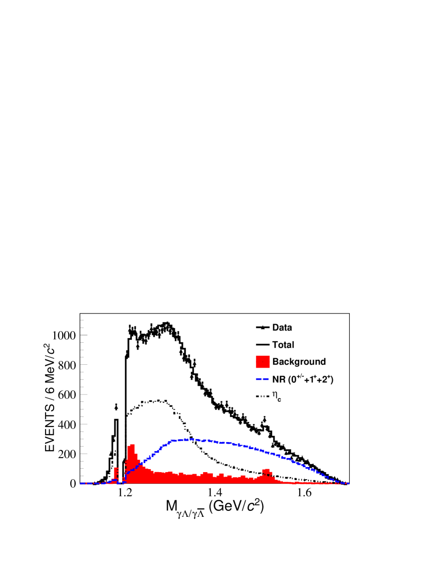
Fig. 6: The invariant mass spectrum $M_{\gamma\Lambda/\gamma\bar{\Lambda}}$ (one event is filled twice by $M_{\gamma\Lambda}$ and $M_{\gamma\bar{\Lambda}})$. The triangles with error bars are data, the black histogram is the total fit result, the red shaded part is the background, the blue dash line is the $NR$ state, and the black dash-dotted line is the signal $\eta_{c}$.

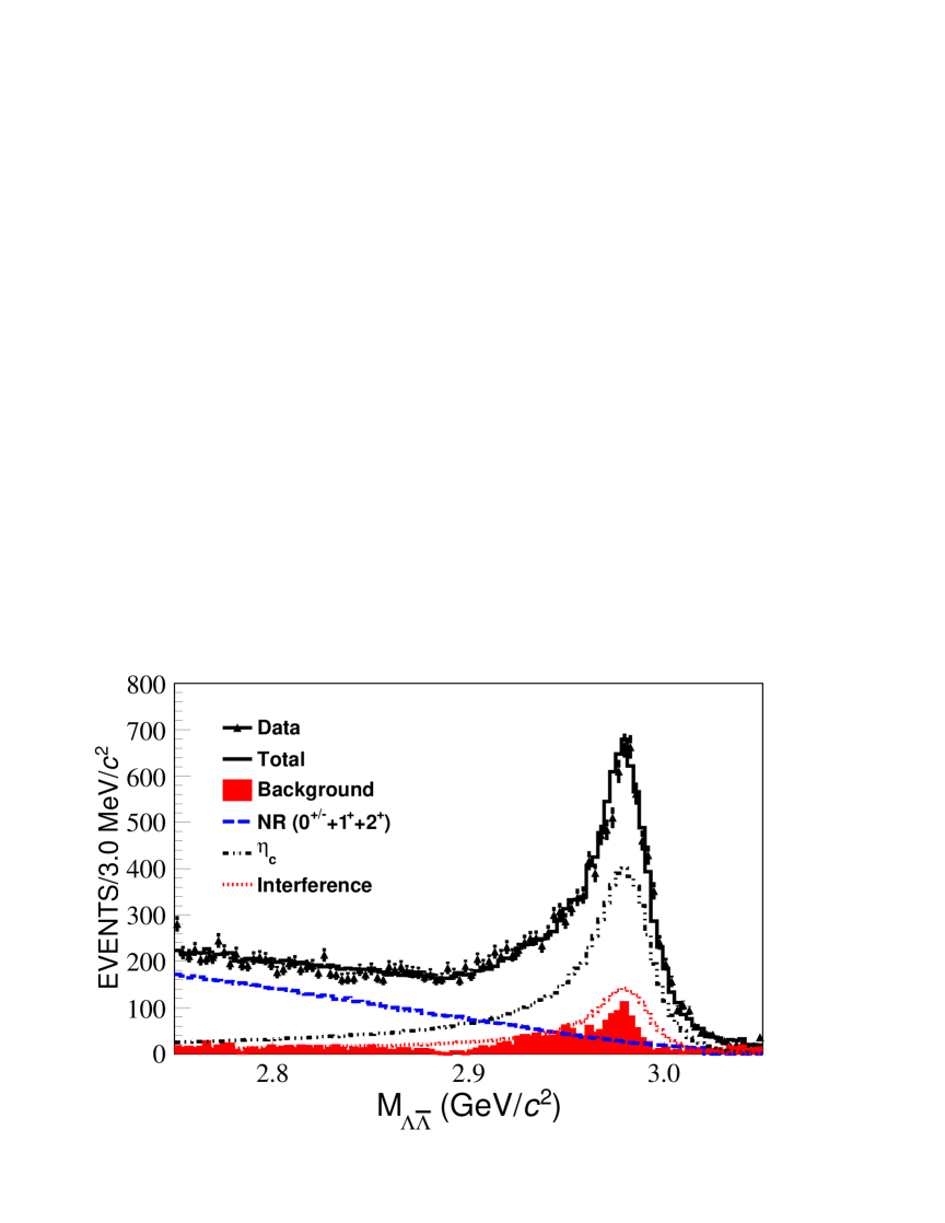
Fig. 7: The invariant mass spectrum $M_{\Lambda\bar{\Lambda}}$. Along with the items described in Fig. 6, the interference of the $\eta_{c}$ with $NR(0^{\pm},1^{+},2^{+})$ is shown.

Figure 8 shows the $\cos\theta_{p\bar{p}}$ distribution. The total histogram is the sum of weighted simulated samples of signal entangled events ($\eta_{c}$ and $NR(0^{-})$), $NR(0^{+},1^{+},2^{+})$, and background. Figure 9 shows the $CH(\theta_{p\bar{p}})$ distribution multiplied by the number of data events. The entries are the number of $\eta_{c}$ signal events in each bin times the value of $CH$ for that bin. The number of signal events is given by the data minus $NR(0^{+},1^{+},2^{+})$ and background.

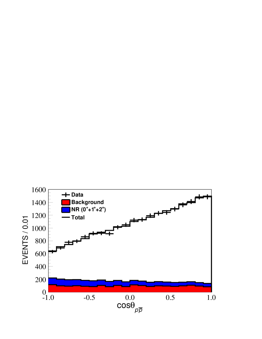
Fig. 8: The angular distribution $\cos\theta_{p\bar{p}}$. The triangles with error bars are data, the histogram is the total fit result, and the shaded areas are the background and non-resonant states.

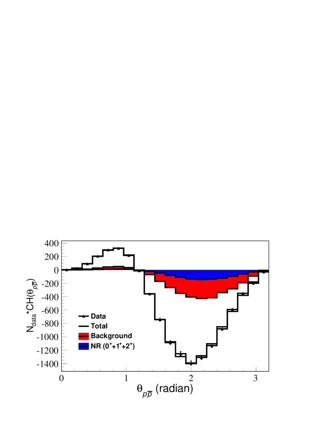
Fig. 9: The distribution of $CH(\theta_{p\bar{p}})=\alpha^{2}_{\Lambda}[\frac{3\cos\theta_{p\bar{p}}-\cos(3\theta_{p\bar{p}})}{4}-\frac{1}{2}]$. The legend is the same as Fig. 8.

The yields of $J^{P}$ components are determined according to the MC event weights, namely, the ratio of cross section for the $J^{P}$ component over the total cross section. Supplementary Table 1 shows the number of yields in data for the $NR(0^{+},0^{-},1^{+},2^{+})$ and $\eta_{c}$ components.

Table 1: The yields of each component determined in the amplitude fit.

Components	$NR(0^{+})$	$NR(1^{+})$	$NR(2^{+})$	$NR(0^{-})$	$\eta_{c}$
Yields	$892.4\pm 230.3$	$116.2\pm 52.8$	$478.5\pm 155.6$	$6139.7\pm 353.2$	$8576.6\pm 154.6$

2.1 Test of Bell inequality

The angular distribution of $p\bar{p}$ is shown in Fig. 10. The points with total error bars, corresponding to signal, are obtained by subtracting the background and the weighted spin-entanglement background events in the amplitude model from the selected events, correcting by the efficiency, then normalizing by the total number of signal events. The dashed line shows the QM prediction with a slope of $\alpha_{\Lambda}^{2}$, we take $\alpha_{\Lambda}=0.750\pm 0.009\pm 0.004$ [41]. The dotted line represents the QM prediction with $\Lambda$ polarization determined by a hidden process, and its slope is $\alpha^{2}_{\Lambda}/3$. The shaded region represents the region that satisfies the Bell inequality of Eq. (3) in the main text. However, the measured angular distribution is outside this region, indicating a significant violation of the Bell inequality, while being consistent with the QM prediction for $\Lambda\bar{\Lambda}$ spin-entanglement events. To assess the significance of distinguishing the QM prediction from the Bell inequality, we fit the measured distribution using a linear combination of both the nearby boundary of the Bell inequality and the QM prediction (refer to Fig. 10), with two parameters. The change in the $\chi^{2}$ of the binned fit, with and without the QM prediction, is 69.2, corresponding to a change of one degree of freedom with consideration of systematic uncertainties. Therefore, the significance to exclude the Bell inequality region is $8.9\sigma$.

\begin{overpic}[width=346.89731pt]{epr.eps} \end{overpic}

Fig. 10: Normalized signal event distribution ($R_{i}=N_{i}/N_{tot}$) of $\cos\theta_{p\bar{p}}$. Here $N_{i}(N_{tot})$ is the number of events in $i$-th bin (total signal events). The points with total error bars are the signal, while the dashed line is the QM prediction, with a slope of $\alpha_{\Lambda}^{2}$. The dotted line represents the QM prediction with $\Lambda$ polarization determined by a hidden process. The filled region indicates the domain that satisfies the Bell inequality (denoted by BI in this figure) in Eq.(3).

2.2 Test of Clauser-Horne-Shimony-Holt inequality

Another type of Bell inequality was proposed based on the CHSH inequality. Utilizing the bilinear expression of the CHSH inequality in momentum space [32], one has

$$|\langle n_{a}n_{b}^{\prime}\rangle+\langle n_{a}n_{d}^{\prime}\rangle+\langle n_{c}n_{b}^{\prime}\rangle-\langle n_{c}n_{d}^{\prime}\rangle|\leq{2\alpha_{\Lambda}^{2}\over 9},$$ (13)

Here, ${\bf n}={\bf p/|p|}$ and ${\bf n^{\prime}}={\bf p^{\prime}/|p^{\prime}|}$, where ${\bf p}$ and ${\bf p^{\prime}}$ represent the momenta of the proton and anti-proton in the rest frames of $\Lambda$ and $\bar{\Lambda}$, respectively. The guide directions are denoted by $a$, $b$, $c$, and $d$, and momentum projections are defined as $\langle n_{a}n_{b}^{\prime}\rangle=\langle{\bf n\cdot a}~{\bf n^{\prime}\cdot d}\rangle$, for example. In the case of maximal violation of the Bell inequality, the momentum correlation can be related to the decay amplitude by defining:

$$C_{ij}\equiv\langle n_{i}n^{\prime}_{j}\rangle{9\over 2\alpha^{2}_{\Lambda}}={9\over 2\alpha^{2}_{\Lambda}|{\bf p}|^{2}}{\int d\Omega_{\Lambda}d\Omega_{p}d\Omega_{\bar{p}}p_{i}p_{j}^{\prime}|\mathcal{M}_{0}|^{2}\over\int d\Omega_{\Lambda}d\Omega_{p}d\Omega_{\bar{p}}|\mathcal{M}_{0}|^{2}},~~~~(i,j=1,2,3)$$ (14)

where the indices $i,j$ label the $x,y,z$ components of a vector in Cartesian coordinates; $\mathcal{M}_{0}$ represents the amplitude for the sequential decay $\eta_{c}\to\Lambda\bar{\Lambda},~\Lambda\to p\pi^{-}$ and $\bar{\Lambda}\to\bar{p}\pi^{+}$. While $C_{ij}$ depends on the QM measurement $\alpha^{2}_{\Lambda}$, it has been demonstrated that the correlation tensor can produce distinct maximum values of $C_{ij}$ for predictions based on QM and local realism (LR), such as:

$$Q_{max}=2\sqrt{C_{11}^{2}+C_{33}^{2}}=\left\{\begin{array}[]{cc}1&(\text{LR})\\ \sqrt{2}&(\text{QM})\end{array}\right..$$ (17)

The LR predicts a maximum value of $Q_{max}=1$, whereas QM can violate local realism with a maximum value of $\sqrt{2}$.

We tested the CHSH inequality by calculating the $C_{ij}$ tensor (see Eq. 14) using the signal of TOY MC events. These events were generated based on the amplitude model with fixed parameters obtained from the amplitude analysis. The statistics of each TOY MC experiment were fixed to those obtained in the amplitude analysis. We then calculated the distribution of $Q_{max}$ according to Eq. 17 as a function of the number of TOY MC experiments, as shown in Fig. 11. The distribution was fitted with a Gaussian function, which provided a good description of the $Q_{max}$ distribution. The mean ($\mu$) and standard deviation ($\sigma$) of the Gaussian distribution were determined to be $\mu=1.416\pm 0.002$ and $\sigma=(2.771\pm 0.001)\times 10^{-2}$, respectively. The $p$-value is calculated with $Q_{max}<1$. Then the significance of vetoing LHVT was estimated to be larger than $10\sigma$.

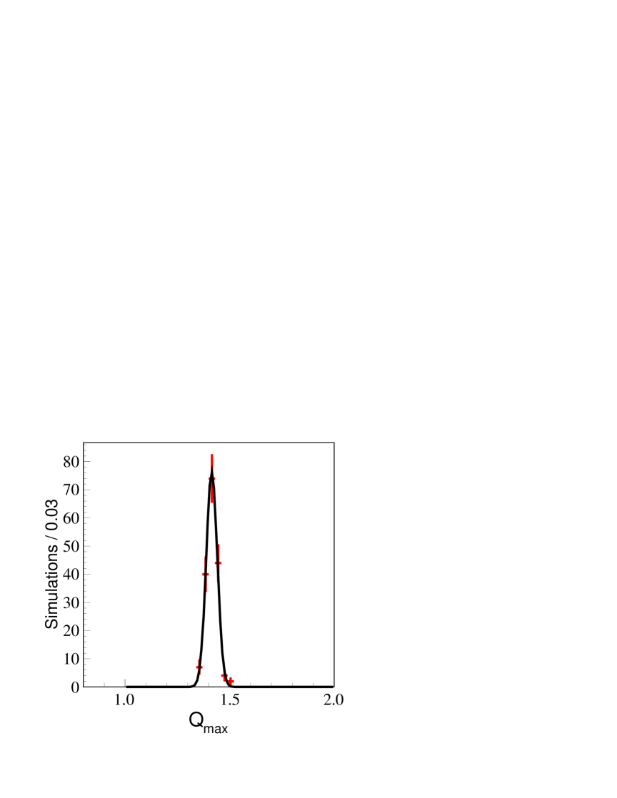
Fig. 11: The distribution of $Q_{max}$ is plotted as a function of the number of TOY MC simulations. The dots with error bars represent the TOY MC results, while the line represents the fitted results using a Gaussian distribution.

Appendix 3 Systematic uncertainties

The systematic uncertainties considered here include: tracking efficiency, photon detection efficiency, space-like separation criteria, kinematic fit, background estimation, and the mass and width of $\eta_{c}$. To account for potential correlations among the systematic sources, all systematic sources, with the exception of the space-like separation, are collectively considered in an alternative fit, rather than being treated separately. Initially, we adjust the MC sample to accommodate the kinematic fit, followed by corrections for tracking efficiency, photon efficiency, and $\Lambda/\bar{\Lambda}$ reconstruction, achieved by multiplying their correction factors to the predicted amplitude squared. The uncertainties in the mass and width of $\eta_{c}$ are factored in when calculating its Breit-Wigner amplitude, by randomly smearing its mass and width. During the subtraction of the background event contribution from the log-likelihood, the weighted factor is smeared in accordance with the statistical uncertainty of the background. The difference in the $\cos\theta_{p\bar{p}}$ distribution between the nominal and alternative fit is considered as the systematic uncertainties. The systematic uncertainties for the $\cos\theta_{p\bar{p}}$ distribution are negligible. However, the systematic uncertainty of the CH inequality distribution is primarily influenced by the space-like separation requirement. The systematic uncertainties are listed as below.

• Tracking efficiency. The tracking efficiencies of $p,\bar{p}$ and $\pi^{\pm}$ are obtained by studying the control sample $J/\psi\to\Lambda\bar{\Lambda}\to p\bar{p}\pi^{+}\pi^{-}$. The event selection criteria of the control sample are the same as those applied in the data analysis. For events with a missing charged track, three charged tracks are identified using PID, and two of the tracks with opposite charge are required to be successfully fitted to a secondary $\Lambda$ vertex. The tracking efficiency of reconstructing a charged track $i$ in data and MC events is defined as: $\varepsilon(i)={N_{\mathrm{trk}=4}\over N_{\mathrm{trk}\geq 3}}$. Here $N_{\mathrm{trk=4}}$ is the number of events for which all four charged tracks are reconstructed, and $N_{\mathrm{trk}\geq 3}$ is the number of events, in which all the other three charged tracks, in addition to the track $i$ to be studied, are reconstructed. The ratio of the efficiency between data and MC events is $R_{\mathrm{trk}}(i)={\varepsilon_{\rm data}(i)\over\varepsilon_{\rm MC}(i)}$. By comparing the control samples, the two-dimensional distributions of $R_{\mathrm{trk}}(p_{t},\cos\theta)$ for $p,\bar{p}$ and $\pi^{\pm}$ are determined, where $p_{t}$ is the transverse momentum. In an alternative fit, the normalization factor $\mathcal{N}(\vec{\xi})$ is multiplied by $R_{\mathrm{trk}}(i)$ for each charged track per event. The difference between the alternative and nominal fits is taken as the systematic uncertainty.

• Photon detection efficiency. The photon detection efficiency is determined by studying the control sample $J/\psi\to\pi^{+}\pi^{-}\pi^{0}$, as done in [59]. The photon selection criteria for the control sample are the same as those used in this analysis. The data selection process requires that each event must contain two oppositely charged tracks and at least one good photon. In cases where an event contains multiple good photons, every combination of $\gamma\pi^{+}\pi^{-}$ is reconstructed. Subsequently, energy conservation is then utilized to pinpoint the region in the EMC where the second photon from $\pi^{0}\to\gamma\gamma$ is expected to be located. The detection efficiency of photons is defined as $\varepsilon_{\gamma}={N_{\gamma\gamma}\over N_{\gamma}}$, where $N_{\gamma\gamma}$ and $N_{\gamma}$ represent the numbers of events in which two photons and one photon appear, respectively. The difference in photon detection efficiencies between data and MC events is determined to be $0.5\%$ and $1.5\%$, corresponding to the barrel and end cap regions of the EMC, respectively. In an alternative fit, the normalization factor $\mathcal{N}(\vec{\xi})$ is calculated by multiplying a Gaussian dispersion factor $\text{Gaus}(1,\delta)$ for each MC event, where $\delta=0.015$ or $0.005$ depending on whether the photon is in the barrel or end cap. The difference between the alternative and nominal fits is taken as the systematic uncertainty.

• Space-like separation criteria. The uncertainty in detection efficiency due to the space-like separation criteria is estimated by the control sample $J/\psi\to\Lambda\bar{\Lambda}$. The event selection criteria of the control sample are the same as those applied in the data analysis. Out of $N$ events, $N^{\prime}$ events satisfy the requirements of the space-like separation criteria, and the selection efficiency is defined as $\epsilon=N^{\prime}/N$. The difference in selection efficiencies between data and MC events is 0.2%, which is negligible.

  However, due to the resolution effect of the detector on the measured decay length of $\Lambda(\bar{\Lambda})$ particles, the space-like separation criteria $L_{1}/L_{2}$ is not uniquely determined. The deviation between the measured value and the true value is determined using MC simulation, where $\Delta(L_{1}/L_{2})$ follows a Gaussian distribution with a mean of 0 and a standard deviation of 0.062 cm. To refine our analysis, we narrowed the window of the $L_{1}/L_{2}$ space-like separation by twice the standard deviation at both ends, and re-selected the data. The difference between the $p\bar{p}$ angular distribution and the CH inequality distribution, obtained by fitting this refined sample, is considered as the systematic uncertainties in comparison to the nominal fitting.

• Kinematic fit. The systematic uncertainty of the 4C kinematic fit is obtained by applying track parameter corrections. The reason for the difference between the kinematic fit of the data and MC events is that the pull distributions of the helix parameters of charged tracks are not consistent. The momentum of the MC event is modified using the pull distribution of the helix parameters. In an alternative fit, we calculate the normalization factor $\mathcal{N}(\vec{\xi})$ with the modified MC events. The difference between the nominal and alternative fits is taken as the systematic uncertainty.

• Background estimation. The number of background events estimated by MC samples for the two simultaneously fitted samples, collected in 2012 and other years, are $1,029\pm 33$ and $3,290\pm 63$. Their statistical fluctuations are used to estimate the uncertainty due to the background. The likelihood function of background events is calculated by multiplying a Gaussian weighting factor $\text{Gaus}(1,\delta n/n)$, where $\delta n/n$ is the relative error of the background. Thus $\ln\mathcal{L}(\vec{\xi},\vec{\omega}_{\rm bg})=\text{Gaus}(1,\delta n/n)\sum_{i=1}^{N_{\rm bg}}\ln\mathcal{P}_{i}(\vec{\xi},\vec{\omega}_{\rm bg})$ is used in an alternative fit.

• $\eta_{c}$ mass and width. In the nominal fit, the $\eta_{c}$ mass and width are fixed to the world averages [53], i.e. $M_{0}=(2983.9\pm 0.4)\text{ MeV}/c^{2}$ and $\Gamma=(32.0\pm 0.7)$ MeV. Their relative uncertainties are $\delta M_{0}/M_{0}=1.7\times 10^{-4}$ and $\delta\Gamma/\Gamma=2.2\%$. The uncertainties are estimated by smearing the $\eta_{c}$ mass and width in the calculation of the likelihood function by a Gaussian distributions, $M_{\eta_{c}}\sim\text{Gaus}(M_{0},\delta M_{0}/M_{0})$ and $\Gamma_{\eta_{c}}\sim\text{Gaus}(\Gamma,\delta\Gamma/\Gamma)$.

References

- [1] Einstein, A. Podolsky, B. & Rosen, N. Can quantum mechanical description of physical reality be considered complete?. Phys. Rev. 47, 777-780 (1935).
- [2] Bohm, D. Quantum Theory (Prentice Hall, New York,1951). p.611.
- [3] Bohm, D. & Aharonov, Y. Discussion of Experimental Proof for the Paradox of Einstein, Rosen, and Podolsky. Phys. Rev. 108, 1070-1076 (1957).
- [4] Bell, J. S. On the Einstein Podolsky Rosen paradox. Physics 1, 195-200 (1964).
- [5] Freedman, S. J. & Clauser, J. F. Experimental test of local hidden-variable theories. Phys. Rev. Lett. 28, 938–941 (1972).
- [6] Aspect, A. Grangier, P. & Roger, G. Experimental tests of realistic local theories via Bell’s theorem. Phys. Rev. Lett. 47, 460–463 (1981).
- [7] Aspect, A. Dalibard, J. & Roger, G. Experimental test of Bell’s inequalities using time-varying analyzers. Phys. Rev. Lett. 49, 1804–1807 (1982).
- [8] Weihs, G. et al. Violation of Bell’s inequality under strict Einstein locality conditions. Phys. Rev. Lett. 81, 5039–5043 (1998).
- [9] Rowe, M. A. et al. Experimental violation of a Bell’s inequality with efficient detection. Nature 409, 791–794 (2001).
- [10] Pan, J. W. Bouwmeester, D. Daniell, M. Weinfurter, H. & Zeilinger, A. Experimental test of quantum nonlocality in three-photon Greenberger-Horne- Zeilinger entanglement. Nature 403, 515–519 (2000).
- [11] Giustina, M. et al. Significant-Loophole-Free Test of Bell’s Theorem with Entangled Photons. Phys. Rev. Lett. 115, 250401 (2015).
- [12] Handsteiner, J. et al. Cosmic Bell Test: Measurement Settings from Milky Way Stars. Phys. Rev. Lett. 118, 060401 (2017)
- [13] Bell, J. S. Speakable and Unspeakable in Quantum Mechanics (Cambridge University Press, Cambridge, 2004). p.232.
- [14] Pearle, P. M. Hidden-variable example based upon data rejection. Phys. Rev. D 2, 1418-1425 (1970).
- [15] Brunner, N. Cavalcanti, D. Pironio, S. Scarani, V. & Wehner, S. Bell nonlocality. Rev. Mod. Phys. 86, 419-478 (2014).
- [16] Larsson, J. Å. Loopholes in Bell inequality tests of local realism. J. Phys. A 47, 424003 (2014).
- [17] Shalm, Lynden K. et al. Strong Loophole-Free Test of Local Realism. Phys. Rev. Lett. 115, 250402 (2015).
- [18] The Nobel Prize in Physics 2022. NobelPrize.org. Nobel Prize Outreach AB 2023. Sun. 30 Apr 2023. <https://www.nobelprize.org/prizes/physics/2022/summary/>.
- [19] Sakai, H. Saito, T. Ikeda, T. et al. Spin correlations of strongly interacting massive fermion pairs as a test of Bell’s inequality[J]. Phys. Rev. Lett. 97, 150405 (2006).
- [20] Bordoloi, A. Zannier, V. Sorba, L. et al. Spin cross-correlation experiments in an electron entangler[J]. Nature, 612 454-458 (2022).
- [21] Colciaghi, P. Li, Y. Treutlein, P & Zibold, T. Einstein-podolsky-rosen experiment with two bose-einstein condensates[J]. Phys. Rev. X, 13 021031 (2023).
- [22] William, K.Wootters. Entanglement of formation of an arbitrary state of two qubits. Phys. Rev. Lett. 80, 2245 (1998).
- [23] Fabbrichesi, M. Floreanini, R. Gabrielli, E & Marzola, L. Bell inequality is violated in charmonium decays. Phys. Rev. D 110, 053008 (2024).
- [24] Li, J. L. & Qiao, C. F. Testing local realism in decays. Sci. China 53, 870 (2010).
- [25] Qian, Ch. Li, J. L. Khan, A. S. & Qiao, C. F. Nonlocal correlation of spin in high energy physics. Phys. Rev. D 101, 116004 (2020).
- [26] Privitera, P. Decay correlations in as a test of quantum mechanics. Phys. Lett. B 275, 172-180 (1992).
- [27] Hao, X. Q. Ke, H. W. D, Y. B. Shen, P. N. & Li, X. Q. Testing Bell Inequality at Experiments of High Energy Physics. Chin. Phys. C 34, 311-318 (2010).
- [28] Chen, X. Wang, S. G. & Mao, Y. J. Understanding polarization correlation of entanged vector meson pairs. Phys. Rev. D 86, 056003 (2012).
- [29] Li, J. L. & Qiao, C. F. Feasibility of testing local hidden variable theories in a Charm factory. Phys. Rev. D 74, 076003 (2006).
- [30] Hiesmayr, B. C. Domenico, A. D. Curceanu, C. Gabriel, A. Huber, M. Larsson, J.-Å. & Moskal, P. Revealing Bell’s Nonlocality for Unstable Systems in High Energy Physics. Eur. Phys. J. C 72, 1856 (2012).
- [31] Baranov, S. P. Bell’s inequality in charmonium decays and . J. Phys. G 35, 075002 (2008).
- [32] Chen, S. Nakaguchi, Y. & Komamiya, S. Testing Bell’s Inequality using Charmonium Decays. Prog. Theor. Exp. P, 063A01 (2013).
- [33] Abel, S. A. Dittmar, M. & Dreiner, H. K. Testing locality at colliders via Bell’s inequality?. Phys. Lett. B 280, 304-312 (1992).
- [34] Belle Collaboration. Observation of Bell inequality violation in B mesons. J. Mod. Opt. 51, 991 (2004).
- [35] Genovese, M. Novero, C. & Predazzi, E. Conclusive tests of local realism and pseudoscalar mesons. Found. Phys. 32, 589-605 (2002).
- [36] Barr, A. J. Fabbrichesi, M. Floreanini, M. Gabrielli E. & Marzola, L. Quantum entanglement and Bell inequality violation at colliders, [arXiv:2402.07972 [hep-ph]].
- [37] Fabbrichesi, M. Floreanini, R. Gabrielli, E.& Marzola,L. Bell inequality is violated in decays. Phys. Rev. D109, L031104(2024).
- [38] Horodecki, R. Horodecki, P. & Horodecki, M. Violating Bell inequality by mixed spin-1/2 states: necessary and sufficient condition. Phys. Lett. A 200, 340-344 (1995).
- [39] Tornqvist, N. A. Suggestion for Einstein-podolsky-rosen Experiments Using Reactions Like . Found. Phys. 11, 171-177 (1981).
- [40] Hiesmayr, B. C. Limits Of Quantum Information In Weak Interaction Processes Of Hyperons. Sci. Rep. 5, 11591 (2015).
- [41] BESIII Collaboration. Polarization and Entanglement in Baryon-Antibaryon Pair Production in Electron-Positron Annihilation. Nature Phys. 15, 631-634 (2019).
- [42] BESIII Collaboration. Precise Measurements of Decay Parameters and CP Asymmetry with Entangled Pairs. Phys. Rev. Lett. 129, 131801 (2022).
- [43] Selleri, F. Quantum Mechanics versus Local Realism: The Einstein, Podolsky, and Rosen Paradox. Plenum Press, New York, 1988.
- [44] Shi, Y. & Yang, J. C. Entangled baryons: violation of Inequalities based on local realism assuming dependence of decays on hidden variables. Eur. Phys. J. C 80, 116 (2020).
- [45] BESIII Collaboration. Design and construction of the BESIII detector. Nucl. Instrum. Meth. A 614, 345 (2010).
- [46] Yu, C. H. et al. BEPCII performance and beam dynamics studies on luminosity. Proceedings of IPAC2016, Busan, Korea, 2016.
- [47] GEANT4 Collaboration. GEANT4–a simulation toolkit. Nucl. Instrum. Meth. Phys. Res. Sect. A 506, 250 (2003).
- [48] Huang, K. X. Li, Z. J. Qian, Z. Zhu, J. Li, H. Y. Zhang, Y. M. Sun, S. S. & You, Z. Y. Method for detector description transformation to Unity and application in BESIII. Nucl. Sci. Tech. 33, 142 (2022).
- [49] Li, Z. J. Yuan, M. K. Song, Y. X. Li, Y. G. Li, J. S. Sun, S. S. Wang, X. L. You, Z. Y. & Mao, Y. J. Visualization for physics analysis improvement and applications in BESIII. Front. Phys. 19, 64201 (2024).
- [50] Jadach, S. Ward, B. F. L. & Was, Z. The precision Monte Carlo event generator K K for two fermion final states in collisions. Comput. Phys. Commun. 130, 260 (2000).
- [51] Lange, D. J. The EvtGen particle decay simulation package. Nucl. Instrum. Meth. A 462, 152 (2001).
- [52] Ping, R. G. Event generators at BESIII. Chin. Phys. C 32, 599 (2008).
- [53] Particle Data Group. Review of Particle Physics. Prog. Theor. Exp. Phys. 083C01 (2022).
- [54] Chen, J. C. Huang, G. S. Qi, X. R. Zhang, D. H. & Zhu, Y. S. Event generator for and decay. Phys. Rev. D 62, 034003 (2000).
- [55] Yang, R. L. Ping, R. G. & Chen, H. Tuning and Validation of the Lundcharm Model with Decays. Chin. Phys. Lett. 31, 061301 (2014).
- [56] BESIII Collaboration. Number of J/ events at BESIII. Chin. Phys. C 46, 074001 (2022).
-
[57]
Chung, S. U. General formulation of covariant helicity-coupling amplitudes. Phys. Rev. D57, 431 (1998);
Chung, S. U. Helicity-coupling amplitudes in tensor formalism. Phys. Rev. D48, 1225 (1993). - [58] JAMES, F. & ROOS, M. Minuit: A system for function minimization and analysis of the parameter errors and correlations. Comput. Phys. Commun. 10, 343 (1975).
- [59] BESIII Collaboration. Amplitude analysis of the system produced in radiative decays. Phys. Rev. D92, 052003 (2015).