Singular Perturbation in Multiscale Stochastic Control Problems with Domain Restriction in the Slow Variable

Abstract

This work investigates multiscale stochastic optimal control problems arising from the integration of intermittent renewable energy sources into the Brazilian power system. We rigorously analyze state-constrained control problems and establish foundational results using viscosity solution theory for degenerate Hamilton–Jacobi–Bellman equations with Neumann-type boundary conditions. A singular perturbation framework is developed to study the convergence of multiscale value functions under infinite-horizon settings. Two examples illustrate the theoretical contributions of the proposed framework.

1 Introduction

In recent years, the substantial expansion of intermittent renewable energy sources, such as solar and wind power, has significantly reshaped the Brazilian energy matrix, as outlined in the 2023–2029 Brazilian Energy Operation Plan and several recent technical studies [LH18, ONS23]. This growth, introduces substantial operational challenges due to the inherently stochastic and multiscale behavior of these sources. Solar generation, for instance, exhibits pronounced intraday variability and is highly sensitive to cloud cover, whereas wind generation is affected by rapidly changing and unpredictable wind patterns. In contrast, hydropower generation follows the seasonal rainfall cycle, which in tropical regions such as Brazil is characterized by alternating wet and dry periods, each lasting approximately six months. These characteristics underscore the necessity for mathematical models capable of accurately capturing both fast and slow dynamics across different time scales in a unified framework.

In this context, Multiscale Stochastic Optimal Control (MSOC) problems emerge as particularly relevant, especially when considering singular perturbations arising from the interaction between fast and slow variables. These problems typically involve systems governed by dynamics evolving over two distinct time scales: a slow variable—such as the seasonal variation in hydrological regimes—and a fast variable capturing the high-frequency fluctuations of solar and wind energy generation. To address the complexity of such systems, dimensionality reduction techniques such as the averaging method are employed, whereby the fast dynamics are replaced by their effective behavior, allowing the retention of essential multiscale features while simplifying the analysis.

An important modeling consideration in energy systems is the restriction of the state space of the slow variable. For instance, when the slow variable represents the water volume in a reservoir, it is naturally confined between minimum and maximum thresholds, i.e., its state space is a bounded polyhedral domain, often idealized as a cube. Analogously, it is reasonable to impose state constraints on the fast variable, for example, when it represents the aggregate generation from wind and solar sources. Developing models that rigorously incorporate both multiscale structures and state constraints over such domains entails numerous theoretical and computational challenges.

In this work, we present a first proof of concept aimed at rigorously analyzing the periodic averaging process in MSOC problems. To streamline the initial investigation, we assume that the state space of the slow variable is a compact, convex domain with a $\text{C}^{2}$ boundary, and that the fast variable evolves on the torus $\mathbb{T}^{d_{Y}}$.

This article is organized as follows:

In Section 2, we study stochastic optimal control problems under state constraints by introducing a cost function associated with maintaining the process within a compact domain with $\text{C}^{2}$ boundary. We allow the dispersion matrix of the reflected controlled stochastic differential equation (SDE) to depend on the control variable and assume that the diffusion matrix is only positive semi-definite. This setting leads to a fully nonlinear, degenerate elliptic second-order Hamilton–Jacobi–Bellman (HJB) equation with a Neumann-type boundary condition. We address this problem within the viscosity solutions framework, and to the best of our knowledge, such a general formulation has not yet been rigorously addressed in the control theory literature.

The most relevant related work we have identified appears in the final chapter of [KD01], where the authors informally outline a viscosity-based approach under more restrictive assumptions: the dispersion matrix is independent of the control and the boundary cost vanishes, leading to a semilinear degenerate elliptic PDE. In contrast, [ABG12], in Chapters 4 and 7, considers this class of problems under the assumption of a strictly positive definite diffusion matrix, thus enabling the use of classical solution techniques.

In Subsection 2.1, we prove the continuity of the associated value function. In Subsection 2.2, we establish the dynamic programming principle (DPP) for strong solutions of reflected controlled SDEs. Finally, in Subsection 2.3, we show that the value function is a viscosity solution of the HJB equation with a Neumann boundary condition, corresponding to the state-constrained control problem.

In Section 3, we focus on singular perturbation problems within the MSOC framework. These fall under the class of dimension reduction problems, as introduced in Chapter 1 of [PS08]. To characterize the core properties of these problems, we adopt the analytical framework of [AB10], which investigates singular perturbations in multiscale stochastic differential games. In contrast, [Kus90] adopts a probabilistic perspective. Our approach is also informed by the works of [BC09], [AB01], and [ABM07], which are the closest in spirit to our investigation, although these studies focus predominantly on finite-horizon problems and do not incorporate boundary cost functions. Our contribution advances the literature by considering infinite-horizon MSOC problems with state constraints on the slow variables.

In Subsection 3.1, we formulate the constrained MSOC problem and demonstrate its well-posedness using the results from Section 2. In Subsection 3.2, we derive the associated effective optimal control problem, again under state constraints, and establish its well-posedness. In Subsection 3.3, we prove the main convergence result of Section 3: the multiscale value function converges uniformly to the effective value function as the time-scale separation parameter tends to zero.

In Section 4, we present two examples that illustrate how the theoretical framework developed in Sections 2 and 3 can be applied. In Subsection 4.1, we consider an MSOC problem with state constraints on the slow variable, where the associated HJB equation is a semilinear degenerate elliptic PDE with boundary conditions. Since the control does not enter the diffusion term, we analyze the function that would define a Markovian control under the hypothetical assumption that classical solutions to the HJB equation exist. In Subsection 4.2, we present an example of a multiscale control problem with constraints on the slow variable, where the control appears in the diffusion of the slow subsystem. This leads to a fully nonlinear, degenerate elliptic HJB equation that encapsulates all the complexities of our framework and, to the best of our knowledge, cannot be addressed within existing frameworks in the literature.

Finally, in Appendices A and B, we present two fundamental analyses in the context of the proposed framework: in Appendix A, we study the differentiability of the Fokker–Planck equation with periodic boundary conditions with respect to the parameters of the slow scale; in Appendix B, we investigate the factorization of the effective diffusion matrix into effective dispersion matrices in a way that preserves their Lipschitz continuity which is a crucial property to be ensured in the analytical approach we develop.

2 Stochastic Optimal Control with Constraints on State Variables

In this section, we analyze a SOC problem in which a constraint is imposed on the state variable. We associate this constraint with a cost function that quantifies the effort—or cost—required to keep the state variable within the desired bounds. Simultaneously, we allow the dispersion matrix of the SDE, whose states we aim to control, to depend on the control variable.

We consider the stochastic basis $\bigg{(}\Omega,\mathcal{O},\big{(}\mathcal{F}_{t}\big{)}_{t\geqslant 0},\mathbb{P}\bigg{)}$ to satisfy the usual conditions; that is, the filtration $\big{(}\mathcal{F}_{t}\big{)}_{t\geqslant 0}$ is right-continuous and contains all $\mathbb{P}$-null sets. Furthermore, $\big{(}W(t)\big{)}_{t\geqslant 0}$ denotes a standard $d_{W}$-dimensional Brownian motion defined on this basis. In the context of strong solutions to SDEs, the filtration, $\big{(}\mathcal{F}_{t}\big{)}_{t\geqslant 0}$ is taken to be the one generated by the Brownian motion, augmented with the $\mathbb{P}$-null sets.

We also fix a compact set $\mathbb{X}\subset\mathbb{R}^{d}$ that will play a key role in our state constraint formulation. Specifically, we assume the existence of a function $\phi\in\text{C}^{2}_{\text{b}}\big{(}\mathbb{R}^{d}\big{)}$ such that:

• $\mathbb{X}=\Bigg{\{}x\in\mathbb{R}^{d}:\phi\big{(}x\big{)}\leqslant 0\Bigg{\}}$;

• $\text{Int}\big{(}\mathbb{X}\big{)}=\Bigg{\{}x\in\mathbb{R}^{d}:\phi\big{(}x\big{)}<0\Bigg{\}}$;

• $\partial\mathbb{X}=\Bigg{\{}x\in\mathbb{R}^{d}:\phi\big{(}x\big{)}=0\Bigg{\}}$ with $\|D_{x}\phi\big{(}x\big{)}\|=1$ for all $x\in\partial\mathbb{X}$.

The dynamical system we aim to control evolves within the constrained state space $\mathbb{X}$ and is governed by the solution of the following SDE with reflection:

$$dX_{x}(t)=\mu_{X}\bigg{(}X_{x}(t),u(t)\bigg{)}dt+\sigma_{X}\bigg{(}X_{x}(t),u(t)\bigg{)}dW(t)-D_{x}\phi\bigg{(}X_{x}(t)\bigg{)}dl_{x}(t).$$ (1)

This equation captures the interplay between the stochastic dynamics of the system and the reflection mechanism that ensures the state remains within the set $\mathbb{X}$. The system is composed of the following elements:

• $\mu_{X}$ and $\sigma_{X}$ represent the drift and dispersion fields, respectively.

• The process $\big{(}X_{x}(t)\big{)}_{t\geqslant 0}$ is continuous and adapted to $\big{(}\mathcal{F}_{t}\big{)}_{t\geqslant 0}$.

• The process $\big{(}l_{x}(t)\big{)}_{t\geqslant 0}$ is continuous, non-decreasing, and adapted to $\big{(}\mathcal{F}_{t}\big{)}_{t\geqslant 0}$. Additionally, we have $l_{x}(0)=0$, and this process satisfies the following condition:

  $$l_{x}(t)=\int_{0}^{t}\mathds{1}_{\partial\mathbb{X}}\bigg{(}X_{x}(s)\bigg{)}dl_{x}(s)\quad\mathbb{P}\text{-a.s.}$$

• The process $\big{(}u(t)\big{)}_{t\geqslant 0}$ is progressively measurable with respect to $\big{(}\mathcal{F}_{t}\big{)}_{t\geqslant 0}$ and takes values in a convex and compact set $\mathbb{U}\subset\mathbb{R}^{m}$. We denote the set of such controls by $\mathcal{U}$, and refer to them as admissible controls.

Remark 1.

The intuitive interpretation of $-D_{x}\phi\big{(}X_{x}(t)\big{)}$ is as follows: this gradient function acts as a force field that reflects the process $\big{(}X_{x}(t)\big{)}_{t\geqslant 0}$ back into the domain $\mathbb{X}$. The reflection is instantaneously triggered by the process $\big{(}l_{x}(t)\big{)}_{t\geqslant 0}$ whenever the state $X_{x}(t)$ reaches the boundary $\partial\mathbb{X}$.

We now introduce the following hypothesis for the drift and dispersion fields:

• The drift $\mu_{X}$ and dispersion $\sigma_{X}$ are continuous, bounded, and Lipschitz continuous with respect to the spatial variable, uniformly with respect to the control variable. Specifically, there exists a constant $C>0$ such that for every $x,y\in\mathbb{R}^{d}$ and every $u\in\mathbb{U}$, the following inequalities hold:

  $$\|\mu_{X}\big{(}x,u\big{)}-\mu_{X}\big{(}y,u\big{)}\|+\|\sigma_{X}\big{(}x,u\big{)}-\sigma_{X}\big{(}y,u\big{)}\|\leqslant C\|x-y\|\quad\text{and}\quad\|\mu_{X}\big{(}x,u\big{)}\|+\|\sigma_{X}\big{(}x,u\big{)}\|\leqslant C.$$

With this hypothesis in place, it is possible to show that the SDE (1) admits a unique strong solution, as demonstrated in [LS84], [PR14], and [Pil14].

To complete the formulation of the model, we now define the cost functional. Specifically, we introduce the operation cost and the preventive cost on the boundary, which we denote by $L$ and $h$, respectively.

• The function $L:\mathbb{R}^{d}\times\mathbb{U}\to\mathbb{R}$ is continuous and bounded in $(x,u)$. Moreover, it is Lipschitz continuous in the spatial variable, uniformly with respect to the control variable. That is, there exists a constant $C>0$ such that for every $x,y\in\mathbb{R}^{d}$ and every $u\in\mathbb{U}$, the following inequalities hold:

  $$\big{|}L\big{(}x,u\big{)}-L\big{(}y,u\big{)}\big{|}\leqslant C\|x-y\|\quad\text{and}\quad\big{|}L\big{(}x,u\big{)}\big{|}\leqslant C.$$

  This function is referred to as the operation cost.

• The function $h:\partial\mathbb{X}\to\mathbb{R}$ is continuous. This function is known as the preventive cost on the boundary.

Given $\beta>0$ and $x\in\mathbb{X}$, we define the cost functional $J^{\beta}_{x}:\mathcal{U}\to\mathbb{R}$ by the following expression:

$$J^{\beta}_{x}\big{(}u\big{)}:=\mathbb{E}\Bigg{[}\int_{0}^{+\infty}e^{-\beta s}L\bigg{(}X_{x}(s),u(s)\bigg{)}ds+\int_{0}^{+\infty}e^{-\beta s}h\bigg{(}X_{x}(s)\bigg{)}dl_{x}(s)\Bigg{]}.$$ (2)

With these definitions in place, we now proceed to the first auxiliary lemma needed for the analysis.

Lemma 1.

Given $u\in\mathcal{U}$, assume that the pair of processes $\big{(}X^{u}(t),l^{u}(t)\big{)}_{t\geqslant 0}$ is a strong solution of the SDE (1). Then, for all $p\geqslant 1$, $T\geqslant 0$ and $x,y\in\mathbb{X}$, the following inequalities hold:

$$\mathbb{E}\Bigg{[}\sup_{r\in[0,T]}\|X^{u}_{x}(r)-X^{u}_{y}(r)\|^{p}\Bigg{]} \leqslant C\exp\bigg{\{}CT\bigg{\}}\|x-y\|^{p},$$ (3a)

$$\mathbb{E}\Bigg{[}\sup_{r\in[0,T]}\|X^{u}_{x}(r)\|^{p}\Bigg{]} \leqslant C\bigg{(}1+T^{p}+\|x\|^{p}\bigg{)},$$ (3b)

$$\mathbb{E}\Bigg{[}\sup_{r\in[0,T]}l^{u}_{x}(r)^{p}\Bigg{]} \leqslant C\big{(}1+T^{p}\big{)},$$ (3c)

where $C>0$ is a constant independent of $u$, $T$, $x$ and $y$.

Proof.

We apply Proposition 4.55 of [PR14] to the pair $\big{(}X^{u}(t),l^{u}(t)\big{)}_{t\geqslant 0}$, which is a strong solution of the SDE (1). The independence of the constant $C>0$ from the control $u\in\mathcal{U}$ follows from hypothesis $\text{H}_{1}$, where the Lipschitz constant and the constants that bound the drift and dispersion fields of the SDE (1) do not depend on the control $u$. ∎

Lemma 2.

The functional $J^{\beta}_{x}:\mathcal{U}\to\mathbb{R}$ is well defined and finite.

Proof.

We have to check the integrability of the following terms:

$$\mathbb{E}\Bigg{[}\int_{0}^{+\infty}e^{-\beta s}\bigg{|}L\bigg{(}X_{x}(s),u(s)\bigg{)}\bigg{|}ds\Bigg{]}<\infty\quad\text{and}\quad\mathbb{E}\Bigg{[}\int_{0}^{+\infty}e^{-\beta s}\bigg{|}h\bigg{(}X_{x}(s)\bigg{)}\bigg{|}dl_{x}(s)\Bigg{]}<\infty.$$

We start with the first expectation. By hypothesis $\text{H}_{2}$ there exists a constant $C_{0}>0$ such that $\big{|}L\big{(}x,u\big{)}\big{|}\leqslant C_{0}$ for all $(x,u)\in\mathbb{R}^{d}\times\mathbb{U}$. This implies, by Fubini’s theorem, that

$$\mathbb{E}\Bigg{[}\int_{0}^{+\infty}e^{-\beta s}\bigg{|}L\bigg{(}X_{x}(s),u(s)\bigg{)}\bigg{|}ds\Bigg{]}=\int_{0}^{+\infty}e^{-\beta s}\mathbb{E}\bigg{[}\bigg{|}L\bigg{(}X_{x}(s),u(s)\bigg{)}\bigg{|}\bigg{]}ds\leqslant\int_{0}^{+\infty}C_{0}e^{-\beta s}ds=\frac{C_{0}}{\beta}.$$ (4)

So this term is bounded. For the second part, we get by hypothesis $\text{H}_{3}$, that there exists a constant $C_{0}>0$ such that $\big{|}h\big{(}x\big{)}\big{|}\leqslant C_{0}$ for all $x\in\partial\mathbb{X}$. By integration by parts and Fatou’s lemma, this implies that

$$\mathbb{E}\Bigg{[}\int_{0}^{+\infty}e^{-\beta s}\bigg{|}h\bigg{(}X_{x}(s)\bigg{)}\bigg{|}dl_{x}(s)\Bigg{]} \leqslant C_{0}\mathbb{E}\Bigg{[}\int_{0}^{+\infty}e^{-\beta s}dl_{x}(s)\Bigg{]}=C_{0}\mathbb{E}\Bigg{[}\liminf_{r\to+\infty}\int_{0}^{r}e^{-\beta s}dl_{x}(s)\Bigg{]}\leqslant C_{0}\liminf_{r\to+\infty}\mathbb{E}\Bigg{[}\int_{0}^{r}e^{-\beta s}dl_{x}(s)\Bigg{]}$$

$$=C_{0}\liminf_{r\to+\infty}\mathbb{E}\Bigg{[}l_{x}(r)e^{-\beta r}+\beta\int_{0}^{r}l_{x}(s)e^{-\beta s}ds\Bigg{]}$$

$$=C_{0}\liminf_{r\to+\infty}\Bigg{\{}e^{-\beta r}\mathbb{E}\big{[}l_{x}(r)\big{]}+\beta\mathbb{E}\Bigg{[}\int_{0}^{r}l_{x}(s)e^{-\beta s}ds\Bigg{]}\Bigg{\}}.$$

By Fubini’s theorem, we get

$$\mathbb{E}\Bigg{[}\int_{0}^{+\infty}e^{-\beta s}\bigg{|}h\bigg{(}X_{x}(s)\bigg{)}\bigg{|}dl_{x}(s)\Bigg{]}\leqslant C_{0}\liminf_{r\to+\infty}\Biggl{\{}e^{-\beta r}\mathbb{E}\big{[}l_{x}(r)\big{]}+\beta\int_{0}^{r}\mathbb{E}\big{[}l_{x}(s)\big{]}e^{-\beta s}ds\Biggr{\}}.$$

On the other hand, by the inequality (3c) (with $p=1$) we have that

$$\mathbb{E}\Bigg{[}\int_{0}^{+\infty}e^{-\beta s}\bigg{|}h\bigg{(}X_{x}(s)\bigg{)}\bigg{|}dl_{x}(s)\Bigg{]} \leqslant C_{0}C\liminf_{r\to+\infty}\Biggl{\{}e^{-\beta r}\big{(}1+r\big{)}+\beta\int_{0}^{r}e^{-\beta s}\big{(}1+s\big{)}ds\Biggr{\}}$$

$$=C_{0}C\lim_{r\to+\infty}\Bigg{(}e^{-\beta r}\big{(}1+r\big{)}+\beta\int_{0}^{r}e^{-\beta s}\big{(}1+s\big{)}ds\Bigg{)}$$

$$=C_{0}C\beta\int_{0}^{+\infty}e^{-\beta s}\big{(}1+s\big{)}ds<\infty$$

where $C>0$ is a constant. In other words, we have the inequality

$$\mathbb{E}\Bigg{[}\int_{0}^{+\infty}e^{-\beta s}\bigg{|}h\bigg{(}X_{x}(s)\bigg{)}\bigg{|}dl_{x}(s)\Bigg{]}\leqslant C_{0}C\beta\int_{0}^{+\infty}e^{-\beta s}\big{(}1+s\big{)}ds.$$ (5)

By the inequalities (4) and (5), for all $u\in\mathcal{U}$,

$$\big{|}J^{\beta}_{x}\big{(}u\big{)}\big{|}\leqslant\frac{C_{0}}{\beta}+C_{0}C\beta\int_{0}^{+\infty}e^{-\beta s}\big{(}1+s\big{)}ds.$$

∎

2.1 Continuity of the Optimal Value Function

The control problem is formulated by minimizing the cost functional (2) over the set of admissible controls $\mathcal{U}$. To begin its solution, we define the optimal value function as follows:

$$v^{\beta}\big{(}x\big{)}:=\inf_{u\in\mathcal{U}}J^{\beta}_{x}\big{(}u\big{)}.$$ (6)

Our goal is to prove that this function is at least continuous in the domain $\mathbb{X}$. Such continuity is required to ensure the validity of the dynamic programming principle, which will be established in section §2.2, and also to enable the application of the viscosity solution concept in section §2.3. To this end, we introduce some notations and definitions.

We say that two processes, $\big{(}X(t)\big{)}_{t\geqslant 0}$ and $\big{(}\widetilde{X}(t)\big{)}_{t\geqslant 0}$, are equivalent if $X$ is a modification of $\widetilde{X}$, that is, for all $t\in\mathbb{R}_{+}$, we have $X(t)=\widetilde{X}(t)$ $\mathbb{P}$-almost surely (i.e., $\mathbb{P}$-a.s.).

Definition 1.

Given $T>0$, $d\in\mathbb{N}$ and $p\in[1,+\infty)$, we denote by $\mathcal{S}^{\emph{p}}_{\emph{d}}\big{(}[0,T]\big{)}$ the space of equivalence classes of the processes $X:[0,T]\times\Omega\to\mathbb{R}^{d}$ that are progressively measurable and

$$\mathbb{E}\Bigg{[}\sup_{t\in[0,T]}\|X(t)\|^{p}\Bigg{]}<\infty.$$

The space $\mathcal{S}^{\text{p}}_{\text{d}}\big{(}[0,T]\big{)}$ can naturally be equipped with the following norm:

$$\|X\|_{\mathcal{S}^{\text{p}}_{\text{d}}\big{(}[0,T]\big{)}}:=\mathbb{E}\Bigg{[}\sup_{t\in[0,T]}\|X(t)\|^{p}\Bigg{]}^{\frac{1}{p}}.$$ (7)

Definition 2.

We denote by $\mathcal{S}^{\emph{p}}_{\emph{d}}\big{(}\mathbb{R}_{+}\big{)}$ the space of equivalence classes of processes $X:\mathbb{R}_{+}\times\Omega\to\mathbb{R}^{d}$ that are progressively measurable and for all $T>0$ the restriction $X|_{[0,T]}\in\mathcal{S}^{\emph{p}}_{\emph{d}}\big{(}[0,T]\big{)}$.

For the space $\mathcal{S}^{\text{p}}_{\text{d}}\big{(}\mathbb{R}_{+}\big{)}$, we consider the following norm:

$$\|X\|_{\mathcal{S}^{\text{p}}_{\text{d}}\big{(}\mathbb{R}_{+}\big{)}}:=\int_{0}^{+\infty}e^{-t}\min\Bigg{\{}1,\|X\|_{\mathcal{S}^{\text{p}}_{\text{d}}\big{(}[0,t]\big{)}}\Bigg{\}}dt.$$ (8)

Lemma 3 (Equicontinuity of the family $\big{(}x\mapsto\big{(}X^{u}_{x}(\cdot),l^{u}_{x}(\cdot)\big{)}\big{)}_{u\in\mathcal{U}}$).

Consider that the pair of processes $\big{(}X^{u}_{x}(t),l^{u}_{x}(t)\big{)}_{t\geqslant 0}$ is the unique strong solution of the SDE (1). Then, for all $p\geqslant 1$, the application

$$\mathbb{X}\ni x\mapsto\big{(}X^{u}_{x}(\cdot),l^{u}_{x}(\cdot)\big{)}\in\mathcal{S}^{\emph{p}}_{\emph{d}}\big{(}\mathbb{R}_{+}\big{)}\times\mathcal{S}^{\emph{p}}_{1}\big{(}\mathbb{R}_{+}\big{)}$$ (9)

is equicontinuous with respect to $u\in\mathcal{U}$.

Proof.

From the inequalities (3b) and (3c) we get that the application (9) is well defined. Given $x,y\in\mathbb{X}$ and $X^{u}_{x}(\cdot),X^{u}_{y}(\cdot)\in\mathcal{S}^{\text{p}}_{\text{d}}\big{(}\mathbb{R}_{+}\big{)}$ it follows from definition 2 that, for all $t\geqslant 0$ the restrictions of these processes to the interval $[0,t]$ belong to the space $\mathcal{S}^{\text{p}}_{\text{d}}\big{(}[0,t]\big{)}$. On the other hand, we have from the inequality (3a) in lemma 1 that

$$\|X^{u}_{x}-X^{u}_{y}\|_{\mathcal{S}^{\emph{p}}_{\emph{d}}\big{(}[0,t]\big{)}}\leqslant\sqrt[p]{Ce^{Ct}}\|x-y\|$$

where $C>0$ is a constant independent of $u\in\mathcal{U}$. By definition 8

$$\sup_{u\in\mathcal{U}}\|X^{u}_{x}-X^{u}_{y}\|_{\mathcal{S}^{\emph{p}}_{\emph{d}}\big{(}\mathbb{R}_{+}\big{)}}\leqslant\int_{0}^{+\infty}e^{-t}\min\Bigg{\{}1,\sqrt[p]{Ce^{Ct}}\|x-y\|\Bigg{\}}dt.$$ (10)

Therefore, by the dominated convergence theorem, the family $\big{(}x\mapsto X^{u}_{x}(\cdot)\big{)}_{u\in\mathcal{U}}$ is equicontinuous.

For $x\mapsto l^{u}_{x}(\cdot)$, we apply Itô’s formula to the function $\phi\in\text{C}^{2}_{\text{b}}\big{(}\mathbb{R}^{d}\big{)}$ which comes from the definition of the domain $\mathbb{X}$ and get

$$\phi\bigg{(}X^{u}_{x}(\cdot)\bigg{)}=\phi\big{(}x\big{)}+ \int_{0}^{\cdot}\sum_{i=1}^{d}\partial_{x_{i}}\phi\bigg{(}X^{u}_{x}(s)\bigg{)}\mu_{X,i}\bigg{(}X^{u}_{x}(s),u(s)\bigg{)}ds-\int_{0}^{\cdot}\|D_{x}\phi\bigg{(}X^{u}_{x}(s)\bigg{)}\|^{2}dl^{u}_{x}(s)$$

$$+ \int_{0}^{\cdot}\frac{1}{2}\sum_{i=1}^{d}\sum_{j=1}^{d}\partial^{2}_{x_{i},x_{j}}\phi\bigg{(}X^{u}_{x}(s)\bigg{)}\big{[}\sigma_{X}\sigma^{\top}_{X}\big{]}_{ij}\bigg{(}X^{u}_{x}(s),u(s)\bigg{)}ds$$ (11)

$$+ \int_{0}^{\cdot}\sum_{i=1}^{d}\sum_{l=1}^{d_{W}}\partial_{x_{i}}\phi\bigg{(}X^{u}_{x}(s)\bigg{)}\sigma_{X,il}\bigg{(}X^{u}_{x}(s),u(s)\bigg{)}dW^{(l)}(s)\quad\mathbb{P}\text{-a.s}.$$

Since the process $\big{(}l^{u}_{x}(t)\big{)}_{t\geqslant 0}$ satisfies the equation

$$l^{u}_{x}(t)=\int_{0}^{t}\mathds{1}_{\partial\mathbb{X}}\bigg{(}X^{u}_{x}(s)\bigg{)}dl^{u}_{x}(s)\quad\mathbb{P}\text{-a.s},$$

the third term on the right-hand side in the equality (11) can be written as

$$l^{u}_{x}(t)=\int_{0}^{t}\|D_{x}\phi\bigg{(}X^{u}_{x}(s)\bigg{)}\|^{2}\mathds{1}_{\partial\mathbb{X}}\bigg{(}X^{u}_{x}(s)\bigg{)}dl^{u}_{x}(s)\quad\mathbb{P}\text{-a.s}.$$

Where equality follows by the definition of the domain $\mathbb{X}$ and $\|D_{x}\phi\big{(}x\big{)}\|=1$ for all $x\in\partial\mathbb{X}$. Denoting by $\mathcal{L}^{u}_{X}:\text{C}_{\text{b}}^{2}\big{(}\mathbb{R}^{d}\big{)}\to\text{C}\big{(}\mathbb{R}^{d}\big{)}$ the differential operator defined by

$$\mathcal{L}^{u}_{X}\varphi\big{(}x\big{)}:=\bigg{\langle}\mu_{X}\big{(}x,u\big{)},D_{x}\varphi\big{(}x\big{)}\bigg{\rangle}+\frac{1}{2}\text{Tr}\Bigg{(}\big{[}\sigma_{X}\sigma^{\top}_{X}\big{]}\big{(}x,u\big{)}D^{2}_{x}\varphi\big{(}x\big{)}\Bigg{)}$$ (12)

it follows from (11) that

$$l^{u}_{x}\big{(}\cdot\big{)}=\int_{0}^{\cdot}\mathcal{L}^{u}_{X}\phi\bigg{(}X^{u}_{x}(s)\bigg{)}ds+\sum_{i=1}^{d}\sum_{l=1}^{d_{W}}\int_{0}^{\cdot}\partial_{x_{i}}\phi\bigg{(}X^{u}_{x}(s)\bigg{)}\sigma_{X,il}\bigg{(}X^{u}_{x}(s),u(s)\bigg{)}dW^{(l)}(s)-\bigg{(}\phi\bigg{(}X^{u}_{x}\big{(}\cdot\big{)}\bigg{)}-\phi\big{(}x\big{)}\bigg{)}\quad\mathbb{P}\text{-a.s}.$$

On the other hand, note that it is possible to develop the term

$$x\mapsto\int_{0}^{\cdot}\mathcal{L}^{u}_{X}\phi\bigg{(}X^{u}_{x}(s)\bigg{)}ds+\sum_{i=1}^{d}\sum_{l=1}^{d_{W}}\int_{0}^{\cdot}\partial_{x_{i}}\phi\bigg{(}X^{u}_{x}(s)\bigg{)}\sigma_{X,il}\bigg{(}X^{u}_{x}(s),u(s)\bigg{)}dW^{(l)}(s),$$ (13)

using classical arguments from stochastic calculus (such as Itô isometry), combined with hypothesis $\text{H}_{1}$ and inequality (10) to obtain the equicontinuity of (13) in $\mathcal{S}^{p}_{1}\big{(}\mathbb{R}_{+}\big{)}$ with respect to $u\in\mathcal{U}$. Thus, we obtain that the family $\big{(}x\mapsto l^{u}_{x}\big{(}\cdot\big{)}\big{)}_{u\in\mathcal{U}}$ is equicontinuous. ∎

We now show that the family $\big{(}x\mapsto J^{\beta}_{x}\big{(}u\big{)}\big{)}_{u\in\mathcal{U}}$ is equicontinuous.

Lemma 4 (Equicontinuity of the family $\big{(}x\mapsto J^{\beta}_{x}\big{(}u\big{)}\big{)}_{u\in\mathcal{U}}$).

Given $\beta>0$ the family of applications $\big{(}x\mapsto J^{\beta}_{x}\big{(}u\big{)}\big{)}_{u\in\mathcal{U}}$ is equicontinuous.

Proof.

Given $x_{0}\in\mathbb{X}$, consider $\big{(}x_{n}\big{)}_{n\geqslant 0}$ a sequence in $\mathbb{X}$ such that $\lim_{n\to\infty}x_{n}=x_{0}$. Let’s prove that

$$\lim_{n\to\infty}\sup_{u\in\mathcal{U}}\big{|}J^{\beta}_{x_{n}}\big{(}u\big{)}-J^{\beta}_{x_{0}}\big{(}u\big{)}\big{|}=0.$$ (14)

From the definition of $J^{\beta}_{x}$ we can write

$$J^{\beta}_{x_{n}}\big{(}u\big{)}=\mathbb{E}\big{[}L^{u}_{n}\big{]}+\mathbb{E}\big{[}H^{u}_{n}\big{]},$$

where:

$$L^{u}_{n}:=\int_{0}^{+\infty}e^{-\beta s}L\bigg{(}X^{u}_{x_{n}}(s),u(s)\bigg{)}ds\quad\text{and}\quad H^{u}_{n}:=\int_{0}^{+\infty}e^{-\beta s}h\bigg{(}X^{u}_{x_{n}}(s)\bigg{)}dl^{u}_{x_{n}}(s).$$

We will divide the proof of the limit (14) into several steps.

• (The family $\big{\{}H^{u}_{n}\big{\}}_{n\geqslant 0}$ is uniformly integrable.) By an analogous argument to the one used in the proof of lemma 2, we have that

  $$\mathbb{E}\bigg{[}\big{|}H^{u}_{n}\big{|}^{2}\bigg{]}\leqslant 2\beta^{2}C_{0}C^{2}\int_{0}^{+\infty}e^{-2\beta s}\big{(}1+s^{2}\big{)}ds=:\gamma<\infty.$$ (15)

  Where the bound we obtain is independent of $u\in\mathcal{U}$. The above inequality implies that

  $$\sup_{n\geqslant 0}\mathbb{E}\bigg{[}\big{|}H^{u}_{n}\big{|}^{2}\bigg{]}<\infty.$$

  Thus, from item 2 of lemma 1.12 of [PR14] (with $p=2$), the family $\big{\{}H^{u}_{n}\big{\}}_{n\geqslant 0}$ is uniformly integrable.

  To finish the proof, we need to show that

  $$\lim_{n\to+\infty}\sup_{u\in\mathcal{U}}\big{|}\mathbb{E}\big{[}L^{u}_{n}\big{]}-\mathbb{E}\big{[}L^{u}_{\infty}\big{]}\big{|}=0\quad\text{and}\quad\lim_{n\to+\infty}\sup_{u\in\mathcal{U}}\big{|}\mathbb{E}\big{[}H^{u}_{n}\big{]}-\mathbb{E}\big{[}H^{u}_{\infty}\big{]}\big{|}=0$$

  where

  $$L^{u}_{\infty}:=\int_{0}^{+\infty}e^{-\beta s}L\bigg{(}X^{u}_{x_{0}}(s),u(s)\bigg{)}ds\quad\text{and}\quad H^{u}_{\infty}:=\int_{0}^{+\infty}e^{-\beta s}h\bigg{(}X^{u}_{x_{0}}(s)\bigg{)}dl^{u}_{x_{0}}(s).$$

• In the first case, ($\big{(}L^{u}_{n}\big{)}_{n\geqslant 0}$ converging to $L^{u}_{\infty}$), consider the auxiliary sequences $\big{(}L^{u}_{n,T}\big{)}_{(n,T)\in\mathbb{N}\times\mathbb{R}_{+}}$ and $\big{(}L^{u}_{\infty,T}\big{)}_{T\in\mathbb{R}_{+}}$ defined respectively by:

  $$L^{u}_{n,T}:=\int_{0}^{T}e^{-\beta s}L\bigg{(}X^{u}_{x_{n}}(s),u(s)\bigg{)}ds\quad\text{and}\quad L^{u}_{\infty,T}:=\int_{0}^{T}e^{-\beta s}L\bigg{(}X^{u}_{x_{0}}(s),u(s)\bigg{)}ds$$

  Based on these sequences, we can write

  $$\big{|}L^{u}_{n}-L^{u}_{\infty}\big{|}\leqslant\big{|}L^{u}_{n}-L^{u}_{n,T}\big{|}+\big{|}L^{u}_{n,T}-L^{u}_{\infty,T}\big{|}+\big{|}L^{u}_{\infty,T}-L^{u}_{\infty}\big{|}\quad\mathbb{P}\text{-a.s}.$$ (16)

  Developing the first part on the right-hand side and recalling that according to hypothesis $\text{H}_{2}$ the operation cost is bounded, it follows that

  $$\big{|}L^{u}_{n}-L^{u}_{n,T}\big{|}=\Bigg{|}\int_{T}^{+\infty}e^{-\beta s}L\bigg{(}X^{u}_{x_{n}}(s),u(s)\bigg{)}ds\Bigg{|}\leqslant\int_{T}^{+\infty}Ce^{-\beta s}ds=\frac{Ce^{-T\beta}}{\beta}\quad\mathbb{P}\text{-a.s}.$$

  Applying expectation to both sides of the above inequality, we get

  $$\mathbb{E}\bigg{[}\big{|}L^{u}_{n}-L^{u}_{n,T}\big{|}\bigg{]}\leqslant\frac{Ce^{-T\beta}}{\beta}.$$

  Then, given $\epsilon>0$ there exists $T_{1}>0$ such that for every $T\geqslant T_{1}$

  $$\sup_{u\in\mathcal{U}}\mathbb{E}\bigg{[}\big{|}L^{u}_{n}-L^{u}_{n,T}\big{|}\bigg{]}\leqslant\frac{Ce^{-T\beta}}{\beta}<\frac{\epsilon}{3}.$$ (17)

  By an analogous argument, there exists $T_{2}>0$ such that for every $T\geqslant T_{2}$

  $$\sup_{u\in\mathcal{U}}\mathbb{E}\bigg{[}\big{|}L^{u}_{\infty,T}-L^{u}_{\infty}\big{|}\bigg{]}\leqslant\frac{Ce^{-T\beta}}{\beta}<\frac{\epsilon}{3}.$$ (18)

  Defining $T_{0}:=\max\big{\{}T_{1},T_{2}\big{\}}$ we write

  $$\big{|}L^{u}_{n,T_{0}}-L^{u}_{\infty,T_{0}}\big{|}\leqslant\int_{0}^{T_{0}}e^{-\beta s}\bigg{|}L\bigg{(}X^{u}_{x_{n}}(s),u(s)\bigg{)}-L\bigg{(}X^{u}_{x_{0}}(s),u(s)\bigg{)}\bigg{|}ds\quad\mathbb{P}\text{-a.s}.$$

  By hypothesis $\text{H}_{2}$, the operation cost $L$ is Lipschitz continuous in the spatial variable, uniformly with respect to the control variable. Therefore, there exists a constant $C>0$ (independent of $u\in\mathcal{U}$) such that

  $$\big{|}L^{u}_{n,T_{0}}-L^{u}_{\infty,T_{0}}\big{|}\leqslant C\int_{0}^{T_{0}}e^{-\beta s}\|X^{u}_{x_{n}}(s)-X^{u}_{x_{0}}(s)\|ds\quad\mathbb{P}\text{-a.s}.$$

  Applying the supremum to the norm that appears in the integrand, we get

  $$\big{|}L^{u}_{n,T_{0}}-L^{u}_{\infty,T_{0}}\big{|}\leqslant\frac{C}{\beta}\bigg{(}1-e^{-T_{0}\beta}\bigg{)}\sup_{r\in[0,T_{0}]}\|X^{u}_{x_{n}}(r)-X^{u}_{x_{0}}(r)\|\quad\mathbb{P}\text{-a.s}.$$

  Now, applying expectation to both sides of the above inequality, it follows from equation (7) for $p=1$ (norm in $\mathcal{S}^{1}_{\text{d}}\big{(}[0,T_{0}]\big{)}$) that

  $$\mathbb{E}\bigg{[}\big{|}L^{u}_{n,T_{0}}-L^{u}_{\infty,T_{0}}\big{|}\bigg{]}\leqslant\frac{C}{\beta}\bigg{(}1-e^{-T_{0}\beta}\bigg{)}\|X^{u}_{x_{n}}-X^{u}_{x_{0}}\|_{\mathcal{S}^{1}_{\text{d}}\big{(}[0,T_{0}]\big{)}}.$$

  From the lemma 3, the application $x\mapsto X^{u}_{x}(\cdot)$ is equicontinuous with respect to $u$ according to the metric induced by the norm (8). Then, since $\lim_{n\to\infty}x_{n}=x_{0}$, given $\epsilon>0$ there exists $n_{0}(T_{0})\in\mathbb{N}$ such that for every $n\geqslant n_{0}(T_{0})$

  $$\sup_{u\in\mathcal{U}}\mathbb{E}\bigg{[}\big{|}L^{u}_{n,T_{0}}-L^{u}_{\infty,T_{0}}\big{|}\bigg{]}\leqslant\frac{\epsilon}{3}.$$ (19)

  Therefore, by combining the inequalities (17), (18) and (19) with the inequality (16) we obtain, for all $n\geqslant n_{0}(T_{0})$, that

  $$\sup_{u\in\mathcal{U}}\mathbb{E}\bigg{[}\big{|}L^{u}_{n}-L^{u}_{\infty}\big{|}\bigg{]}\leqslant\epsilon.$$

  This implies that

  $$\lim_{n\to\infty}\sup_{u\in\mathcal{U}}\big{|}\mathbb{E}\big{[}L^{u}_{n}\big{]}-\mathbb{E}\big{[}L^{u}_{\infty}\big{]}\big{|}=0.$$

• We want to use proposition 1.20 of [PR14] , to prove that

  $$\lim_{n\to+\infty}\sup_{u\in\mathcal{U}}\big{|}\mathbb{E}\big{[}H^{u}_{n}\big{]}-\mathbb{E}\big{[}H^{u}_{\infty}\big{]}\big{|}=0.$$

  Similarly to what we did in the first case, we define the auxiliary sequences $\big{(}H^{u}_{n,T}\big{)}_{(n,T)\in\mathbb{N}\times\mathbb{R}_{+}}$ and $\big{(}H^{u}_{\infty,T}\big{)}_{T\in\mathbb{R}_{+}}$ respectively by:

  $$H^{u}_{n,T}:=\int_{0}^{T}e^{-\beta s}h\bigg{(}X^{u}_{x_{n}}(s)\bigg{)}dl^{u}_{x_{n}}(s)\quad\text{and}\quad H^{u}_{\infty,T}:=\int_{0}^{T}e^{-\beta s}h\bigg{(}X^{u}_{x_{0}}(s)\bigg{)}dl^{u}_{x_{0}}(s).$$

  Based on these sequences, we obtain

  $$\big{|}H^{u}_{n}-H^{u}_{\infty}\big{|}\leqslant\big{|}H^{u}_{n}-H^{u}_{n,T}\big{|}+\big{|}H^{u}_{n,T}-H^{u}_{\infty,T}\big{|}+\big{|}H^{u}_{\infty,T}-H^{u}_{\infty}\big{|}\quad\mathbb{P}\text{-a.s}.$$

  Let’s estimate the first term on the right in the inequality above. By hypothesis $\text{H}_{3}$, the preventive cost on the boundary is bounded, then there exists a constant $C>0$ such that, $\big{|}h\big{(}x\big{)}\big{|}\leqslant C$ for all $x\in\partial\mathbb{X}$. Fatou’s lemma and integration by parts imply that

  $$\mathbb{E}\bigg{[}\big{|}H^{u}_{n}-H^{u}_{n,T}\big{|}\bigg{]} \leqslant\mathbb{E}\Bigg{[}\int_{T}^{+\infty}e^{-\beta s}\bigg{|}h\bigg{(}X^{u}_{x_{n}}(s)\bigg{)}\bigg{|}dl^{u}_{x_{n}}(s)\Bigg{]}\leqslant C\mathbb{E}\Bigg{[}\int_{T}^{+\infty}e^{-\beta s}dl^{u}_{x_{n}}(s)\Bigg{]}$$

  $$=C\mathbb{E}\Bigg{[}\liminf_{r\to+\infty}\int_{T}^{r}e^{-\beta s}dl^{u}_{x_{n}}(s)\Bigg{]}\leqslant C\liminf_{r\to+\infty}\mathbb{E}\Bigg{[}\int_{T}^{r}e^{-\beta s}dl^{u}_{x_{n}}(s)\Bigg{]}$$

  $$=C\liminf_{r\to+\infty}\mathbb{E}\Bigg{[}\Bigg{(}l^{u}_{x_{n}}(r)e^{-\beta r}-l^{u}_{x_{n}}(T)e^{-\beta T}\Bigg{)}+\beta\int_{T}^{r}l^{u}_{x_{n}}(s)e^{-\beta s}ds\Bigg{]}$$

  $$=C\liminf_{r\to+\infty}\Bigg{\{}\mathbb{E}\Bigg{[}l^{u}_{x_{n}}(r)e^{-\beta r}-l^{u}_{x_{n}}(T)e^{-\beta T}\Bigg{]}+\beta\mathbb{E}\Bigg{[}\int_{T}^{r}l^{u}_{x_{n}}(s)e^{-\beta s}ds\Bigg{]}\Bigg{\}}.$$

  Since $-l^{u}_{x_{n}}(T)e^{-\beta T}\leqslant 0$ $\mathbb{P}$-a.s it follows that

  $$\mathbb{E}\bigg{[}\big{|}H^{u}_{n}-H^{u}_{n,T}\big{|}\bigg{]}\leqslant C\liminf_{r\to+\infty}\Biggl{\{}e^{-\beta r}\mathbb{E}\bigg{[}l^{u}_{x_{n}}(r)\bigg{]}+\beta\mathbb{E}\Bigg{[}\int_{T}^{r}l^{u}_{x_{n}}(s)e^{-\beta s}ds\Bigg{]}\Biggr{\}}.$$

  By Fubini’s theorem and the inequality (3c) we obtain that

  $$\mathbb{E}\bigg{[}\big{|}H^{u}_{n}-H^{u}_{n,T}\big{|}\bigg{]}\leqslant CC_{0}\liminf_{r\to+\infty}\Biggl{\{}e^{-\beta r}\big{(}1+r\big{)}+\beta\int_{T}^{r}e^{-\beta s}\big{(}1+s\big{)}ds\Biggr{\}}.$$

  This implies that

  $$\big{|}\mathbb{E}\big{[}H^{u}_{n}\big{]}-\mathbb{E}\big{[}H^{u}_{n,T}\big{]}\big{|}\leqslant C_{0}C\beta\int_{T}^{+\infty}e^{-\beta s}\big{(}1+s\big{)}ds.$$

  Now, given $\epsilon>0$ there exists $T_{1}>0$ such that for every $T\geqslant T_{1}$

  $$\sup_{u\in\mathcal{U}}\big{|}\mathbb{E}\big{[}H^{u}_{n}\big{]}-\mathbb{E}\big{[}H^{u}_{n,T}\big{]}\big{|}\leqslant\frac{\epsilon}{3}.$$ (20)

  By an analogous argument, there exists $T_{2}>0$ such that for every $T\geqslant T_{2}$

  $$\sup_{u\in\mathcal{U}}\big{|}\mathbb{E}\big{[}H^{u}_{\infty,T}\big{]}-\mathbb{E}\big{[}H^{u}_{\infty}\big{]}\big{|}\leqslant\frac{\epsilon}{3}.$$ (21)

  On the other hand, defining $T_{0}:=\max\big{\{}T_{1},T_{2}\big{\}}$ and given $\eta>0$, we have by Markov’s inequality

  $$\mathbb{P}\Bigg{(}\|X^{u}_{x_{n}}-X^{u}_{x_{0}}\|_{T_{0}}\geqslant\eta\Bigg{)} \leqslant\frac{1}{\eta}\mathbb{E}\bigg{[}\|X^{u}_{x_{n}}-X^{u}_{x_{0}}\|_{T_{0}}\bigg{]}=\frac{1}{\eta}\|X^{u}_{x_{n}}-X^{u}_{x_{0}}\|_{\mathcal{S}^{1}_{\text{d}}\big{(}[0,T_{0}]\big{)}},$$

  $$\mathbb{P}\Bigg{(}\|l^{u}_{x_{n}}-l^{u}_{x_{0}}\|_{T_{0}}\geqslant\eta\Bigg{)} \leqslant\frac{1}{\eta}\mathbb{E}\bigg{[}\|l^{u}_{x_{n}}-l^{u}_{x_{0}}\|_{T_{0}}\bigg{]}=\frac{1}{\eta}\|l^{u}_{x_{n}}-l^{u}_{x_{0}}\|_{\mathcal{S}^{1}_{1}\big{(}[0,T_{0}]\big{)}}.$$

  Which implies

  $$\sup_{u\in\mathcal{U}}\mathbb{P}\Bigg{(}\|X^{u}_{x_{n}}-X^{u}_{x_{0}}\|_{T_{0}}\geqslant\eta\Bigg{)} \leqslant\frac{1}{\eta}\sup_{u\in\mathcal{U}}\|X^{u}_{x_{n}}-X^{u}_{x_{0}}\|_{\mathcal{S}^{1}_{\text{d}}\big{(}[0,T_{0}]\big{)}},$$

  $$\sup_{u\in\mathcal{U}}\mathbb{P}\Bigg{(}\|l^{u}_{x_{n}}-l^{u}_{x_{0}}\|_{T_{0}}\geqslant\eta\Bigg{)} \leqslant\frac{1}{\eta}\sup_{u\in\mathcal{U}}\|l^{u}_{x_{n}}-l^{u}_{x_{0}}\|_{\mathcal{S}^{1}_{1}\big{(}[0,T_{0}]\big{)}}.$$

  Since $\lim_{n\to+\infty}x_{n}=x_{0}$, it follows by the lemma 3 (equicontinuity with respect to u of the applications $x\mapsto X^{u}_{x}\big{(}\cdot\big{)}$ and $x\mapsto l^{u}_{x}\big{(}\cdot\big{)}$), that

  $$\lim_{n\to+\infty}\sup_{u\in\mathcal{U}}\mathbb{P}\Bigg{(}\|X^{u}_{x_{n}}-X^{u}_{x_{0}}\|_{T_{0}}\geqslant\eta\Bigg{)}=0\quad\text{and}\quad\lim_{n\to+\infty}\sup_{u\in\mathcal{U}}\mathbb{P}\Bigg{(}\|l^{u}_{x_{n}}-l^{u}_{x_{0}}\|_{T_{0}}\geqslant\eta\Bigg{)}=0.$$

  Then, the sequences $\big{(}\|X^{u}_{x_{n}}-X^{u}_{x_{0}}\|_{T_{0}}\big{)}_{n\geqslant 0}$ and $\big{(}\|l^{u}_{x_{n}}-l^{u}_{x_{0}}\|_{T_{0}}\big{)}_{n\geqslant 0}$ converge to zero in probability uniformly in $u\in\mathcal{U}$. This implies that the sequence $\big{(}\|X^{u}_{x_{n}}-X^{u}_{x_{0}}\|_{T_{0}}+\|l^{u}_{x_{n}}-l^{u}_{x_{0}}\|_{T_{0}}\big{)}_{n\geqslant 0}$ also converges to zero in probability uniformly in $u\in\mathcal{U}$. By the inequality (3c) we have, for $p=1$, that

  $$\lambda:=\sup_{n\geqslant 0}\mathbb{E}\bigg{[}l^{u}_{x_{n}}\big{(}T_{0}\big{)}\bigg{]}\leqslant C_{0}\big{(}1+T_{0}\big{)}<\infty.$$

  Then, by proposition 1.20 of [PR14], it follows that

  $$H^{u}_{n,T_{0}}=\int_{0}^{T_{0}}e^{-\beta s}h\bigg{(}X^{u}_{x_{n}}(s)\bigg{)}dl^{u}_{x_{n}}(s)\to\int_{0}^{T_{0}}e^{-\beta s}h\bigg{(}X^{u}_{x_{0}}(s)\bigg{)}dl^{u}_{x_{0}}(s)=H^{u}_{\infty,T_{0}}$$

  in probability uniformly in $u\in\mathcal{U}$. Consequently, the sequence $\big{(}H^{u}_{n,T_{0}}\big{)}_{n\geqslant 0}$ converges in distribution to $H^{u}_{\infty,T_{0}}$ uniformly in $u\in\mathcal{U}$. Since the family $\big{\{}H^{u}_{n,T_{0}}\big{\}}_{n\geqslant 0}$ is uniformly integrable, it follows, by theorem 1.15 of [PR14], that given $\epsilon>0$ there exists $n_{0}(T_{0})\in\mathbb{N}$ such that for every $n\geqslant n_{0}(T_{0})$

  $$\sup_{u\in\mathcal{U}}\big{|}\mathbb{E}\big{[}H^{u}_{n,T_{0}}\big{]}-\mathbb{E}\big{[}H^{u}_{\infty,T_{0}}\big{]}\big{|}<\frac{\epsilon}{3}.$$ (22)

  Combining the inequalities (20), (21) and (22), we get

  $$\sup_{u\in\mathcal{U}}\big{|}\mathbb{E}\big{[}H^{u}_{n}\big{]}-\mathbb{E}\big{[}H^{u}_{\infty}\big{]}\big{|}<\epsilon.$$

• (Conclusion) Finally, we get

  $$\lim_{n\to+\infty}\sup_{u\in\mathcal{U}}\big{|}J^{\beta}_{x_{n}}\big{(}u\big{)}-J^{\beta}_{x_{0}}\big{(}u\big{)}\big{|}\leqslant\lim_{n\to+\infty}\sup_{u\in\mathcal{U}}\big{|}\mathbb{E}\big{[}L^{u}_{n}\big{]}-\mathbb{E}\big{[}L^{u}_{\infty}\big{]}\big{|}+\lim_{n\to+\infty}\sup_{u\in\mathcal{U}}\big{|}\mathbb{E}\big{[}H^{u}_{n}\big{]}-\mathbb{E}\big{[}H^{u}_{\infty}\big{]}\big{|}=0.$$

  We conclude that the family $\big{(}x\mapsto J^{\beta}_{x}\big{(}u\big{)}\big{)}_{u\in\mathcal{U}}$ is equicontinuous.

∎

Theorem 1 (Continuity of the Optimal Value Function).

The Optimal Value Function (6) is continuous.

Proof.

On the one hand, given $x_{0},x\in\mathbb{X}$, we have that

$$-J^{\beta}_{x}\big{(}\widetilde{u}\big{)} =J^{\beta}_{x_{0}}\big{(}\widetilde{u}\big{)}-J^{\beta}_{x}\big{(}\widetilde{u}\big{)}-J^{\beta}_{x_{0}}\big{(}\widetilde{u}\big{)}\leqslant\big{|}J^{\beta}_{x_{0}}\big{(}\widetilde{u}\big{)}-J^{\beta}_{x}\big{(}\widetilde{u}\big{)}\big{|}-J^{\beta}_{x_{0}}\big{(}\widetilde{u}\big{)}$$

$$\leqslant\sup_{u\in\mathcal{U}}\big{|}J^{\beta}_{x_{0}}\big{(}u\big{)}-J^{\beta}_{x}\big{(}u\big{)}\big{|}+\sup_{u\in\mathcal{U}}\biggl{\{}-J^{\beta}_{x_{0}}\big{(}u\big{)}\biggr{\}}$$

$$=\sup_{u\in\mathcal{U}}\big{|}J^{\beta}_{x_{0}}\big{(}u\big{)}-J^{\beta}_{x}\big{(}u\big{)}\big{|}-\inf_{u\in\mathcal{U}}J^{\beta}_{x_{0}}\big{(}u\big{)}.$$

The above inequality implies

$$-\inf_{u\in\mathcal{U}}J^{\beta}_{x}\big{(}u\big{)}=\sup_{u\in\mathcal{U}}\biggl{\{}-J^{\beta}_{x}\big{(}u\big{)}\biggr{\}}\leqslant\sup_{u\in\mathcal{U}}\big{|}J^{\beta}_{x_{0}}\big{(}u\big{)}-J^{\beta}_{x}\big{(}u\big{)}\big{|}-\inf_{u\in\mathcal{U}}J^{\beta}_{x_{0}}\big{(}u\big{)}.$$

In other words,

$$\inf_{u\in\mathcal{U}}J^{\beta}_{x_{0}}\big{(}u\big{)}-\inf_{u\in\mathcal{U}}J^{\beta}_{x}\big{(}u\big{)}\leqslant\sup_{u\in\mathcal{U}}\big{|}J^{\beta}_{x_{0}}\big{(}u\big{)}-J^{\beta}_{x}\big{(}u\big{)}\big{|}.$$

On the other hand, since the argument is symmetrical, it follows that

$$\inf_{u\in\mathcal{U}}J^{\beta}_{x}\big{(}u\big{)}-\inf_{u\in\mathcal{U}}J^{\beta}_{x_{0}}\big{(}u\big{)}\leqslant\sup_{u\in\mathcal{U}}\big{|}J^{\beta}_{x_{0}}\big{(}u\big{)}-J^{\beta}_{x}\big{(}u\big{)}\big{|}.$$

Thus, we get

$$\big{|}v^{\beta}\big{(}x_{0}\big{)}-v^{\beta}\big{(}x\big{)}\big{|}=\Bigg{|}\inf_{u\in\mathcal{U}}J^{\beta}_{x_{0}}\big{(}u\big{)}-\inf_{u\in\mathcal{U}}J^{\beta}_{x}\big{(}u\big{)}\Bigg{|}\leqslant\sup_{u\in\mathcal{U}}\big{|}J^{\beta}_{x_{0}}\big{(}u\big{)}-J^{\beta}_{x}\big{(}u\big{)}\big{|}.$$

By the lemma 4 given $\epsilon>0$ there exists $\delta_{x_{0}}(\epsilon)>0$ such that

$$\|x_{0}-x\|\leqslant\delta_{x_{0}}(\epsilon)\Rightarrow\sup_{u\in\mathcal{U}}\big{|}J^{\beta}_{x_{0}}\big{(}u\big{)}-J^{\beta}_{x}\big{(}u\big{)}\big{|}<\epsilon.$$

This implies

$$\|x_{0}-x\|\leqslant\delta_{x_{0}}(\epsilon)\Rightarrow\big{|}v^{\beta}\big{(}x_{0}\big{)}-v^{\beta}\big{(}x\big{)}\big{|}<\epsilon.$$

∎

2.2 The Dynamic Programming Principle

Dynamic programming is a widely used methodology for solving problems involving multi-stage or sequential decision-making in discrete time; see, for example, Chapter 12 of [PIL09] and Chapter 4 of [Koc15]. This methodology relies on an optimality principle known as the Dynamic Programming Principle (DPP). For a thorough theoretical development, see [Ber18]; for a discussion on the practical challenges and algorithmic implementations, refer to [Pow11].

The DPP can also be extended to continuous-time decision problems, such as those arising in optimal control theory. In the deterministic setting, its mathematical formulation is relatively straightforward; see, for instance, Lemma 202 in Chapter 12 of [BL14]. However, in the stochastic setting, the DPP becomes a highly technical result. The level of complexity depends on the nature of the control strategies considered. For example, if feedback-type controls are used, then strong solutions to the controlled SDE (1) may exist only in very specific situations.

Before presenting the main result, we make a few additional remarks. The admissible controls under consideration are adapted to the filtration $\big{(}\mathcal{F}_{t}\big{)}_{t\geqslant 0}$, which is the completion of the filtration generated by the Brownian motion. Consequently, these controls can be represented as measurable functions of the Brownian motion’s trajectory. This leads, by arguments similar to those in Theorem 8.5 of Chapter 8 of [Gal14], to the existence of measurable functions $\mathfrak{X}$ and $\mathfrak{L}$ such that

$$X^{u}_{x}(t)=\mathfrak{X}^{u}_{x}\big{(}W\big{)}(t)\quad\text{and}\quad l^{u}_{x}(t)=\mathfrak{L}^{u}_{x}\big{(}W\big{)}(t).$$

Thus, given a stopping time $\tau:\Omega\to\mathbb{R}_{+}$ with respect to $\big{(}\mathcal{F}_{t}\big{)}_{t\geqslant 0}$ and the $\sigma$-algebra

$$\mathcal{F}_{\tau}:=\Bigg{\{}A\in\mathcal{O}:\big{\{}\tau\leqslant t\big{\}}\cap A\in\mathcal{F}_{t},\hskip 4.26773pt\forall t\in\mathbb{R}_{+}\Bigg{\}},$$

the following equality holds

$$\mathbb{E}\Bigg{[}\int_{\tau}^{+\infty}e^{-\beta(s-\tau)}L\bigg{(}X_{X_{x}(\tau)}(s),u(s)\bigg{)}ds+\int_{\tau}^{+\infty}e^{-\beta(s-\tau)}h\bigg{(}X_{X_{x}(\tau)}(s)\bigg{)}dl_{X_{x}(\tau)}(s)\Bigg{|}\mathcal{F}_{\tau}\Bigg{]}=J^{\beta}_{X_{x}(\tau)}\big{(}\widetilde{u}\big{)}\quad\mathbb{P}\text{-a.s}$$

where $\widetilde{u}$ is the restriction of the control $u$ to the interval $[\tau,+\infty)$. The above result can also be obtained, by a convenient adaptation of lemma 3.2 from Chapter 4 of [YZ99].

For the case with an infinite horizon and reflection on the boundary we have.

Theorem 2 (Dynamic Programming Principle).

Consider hypotheses $\emph{H}_{1}$, $\emph{H}_{2}$ and $\emph{H}_{3}$. Then, for all $x\in\mathbb{X}$

$$v^{\beta}\big{(}x\big{)}=\inf_{u\in\mathcal{U}}\inf_{\tau\in\mathcal{T}}\mathbb{E}\Bigg{[} \int_{0}^{\tau}e^{-\beta s}L\bigg{(}X_{x}(s),u(s)\bigg{)}ds+\int_{0}^{\tau}e^{-\beta s}h\bigg{(}X_{x}(s)\bigg{)}dl_{x}(s)+e^{-\beta\tau}v^{\beta}\bigg{(}X_{x}(\tau)\bigg{)}\Bigg{]}$$ (23a)

$$=\inf_{u\in\mathcal{U}}\sup_{\tau\in\mathcal{T}}\mathbb{E}\Bigg{[} \int_{0}^{\tau}e^{-\beta s}L\bigg{(}X_{x}(s),u(s)\bigg{)}ds+\int_{0}^{\tau}e^{-\beta s}h\bigg{(}X_{x}(s)\bigg{)}dl_{x}(s)+e^{-\beta\tau}v^{\beta}\bigg{(}X_{x}(\tau)\bigg{)}\Bigg{]},$$ (23b)

where $\mathcal{T}$ is the set of stopping times with respect to $\big{(}\mathcal{F}_{t}\big{)}_{t\geqslant 0}$. In addition, we adopt the convention that $e^{-\beta\tau(\omega)}=0$ for all $\omega\in\Omega$ such that $\tau(\omega)=+\infty$.

Proof.

According to hypotheses $\text{H}_{1}$, $\text{H}_{2}$ and $\text{H}_{3}$, the three processes that appear in equations (23a) and (23b) are measurable and bounded, so the expectation is well defined. Given $x\in\mathbb{X}$ and $u\in\mathcal{U}$, it follows from the conditional expectation property that

$$J^{\beta}_{x}\big{(}u\big{)}=\mathbb{E}\Bigg{[} \int_{0}^{+\infty}e^{-\beta s}L\bigg{(}X_{x}(s),u(s)\bigg{)}ds+\int_{0}^{+\infty}e^{-\beta s}h\bigg{(}X_{x}(s)\bigg{)}dl_{x}(s)\Bigg{]}$$

$$=\mathbb{E}\Bigg{[} \int_{0}^{\tau}e^{-\beta s}L\bigg{(}X_{x}(s),u(s)\bigg{)}ds+\int_{0}^{\tau}e^{-\beta s}h\bigg{(}X_{x}(s)\bigg{)}dl_{x}(s)$$

$$+e^{-\beta\tau}\mathbb{E}\Bigg{[}\int_{\tau}^{+\infty}e^{-\beta(s-\tau)}L\bigg{(}X_{x}(s),u(s)\bigg{)}ds+\int_{\tau}^{+\infty}e^{-\beta(s-\tau)}h\bigg{(}X_{x}(s)\bigg{)}dl_{x}(s)\Bigg{|}\mathcal{F}_{\tau}\Bigg{]}\Bigg{]}$$

$$=\mathbb{E}\Bigg{[} \int_{0}^{\tau}e^{-\beta s}L\bigg{(}X_{x}(s),u(s)\bigg{)}ds+\int_{0}^{\tau}e^{-\beta s}h\bigg{(}X_{x}(s)\bigg{)}dl_{x}(s)$$

$$+e^{-\beta\tau}\mathbb{E}\Bigg{[}\int_{\tau}^{+\infty}e^{-\beta(s-\tau)}L\bigg{(}X_{X_{x}(\tau)}(s),u(s)\bigg{)}ds+\int_{\tau}^{+\infty}e^{-\beta(s-\tau)}h\bigg{(}X_{X_{x}(\tau)}(s)\bigg{)}dl_{X_{x}(\tau)}(s)\Bigg{|}\mathcal{F}_{\tau}\Bigg{]}\Bigg{]}$$

$$=\mathbb{E}\Bigg{[} \int_{0}^{\tau}e^{-\beta s}L\bigg{(}X_{x}(s),u(s)\bigg{)}ds+\int_{0}^{\tau}e^{-\beta s}h\bigg{(}X_{x}(s)\bigg{)}dl_{x}(s)+e^{-\beta\tau}J^{\beta}_{X_{x}(\tau)}\big{(}\widetilde{u}\big{)}\Bigg{]}$$

where $\widetilde{u}$ is the restriction of the control $u$ to the interval $[\tau,+\infty)$. Since $v^{\beta}\bigg{(}X_{x}(\tau)\bigg{)}\leqslant J^{\beta}_{X_{x}(\tau)}\big{(}\widetilde{u}\big{)}$ $\mathbb{P}$-a.s, we have that

$$J^{\beta}_{x}\big{(}u\big{)}\geqslant\mathbb{E}\Bigg{[}\int_{0}^{\tau}e^{-\beta s}L\bigg{(}X_{x}(s),u(s)\bigg{)}ds+\int_{0}^{\tau}e^{-\beta s}h\bigg{(}X_{x}(s)\bigg{)}dl_{x}(s)+e^{-\beta\tau}v^{\beta}\bigg{(}X_{x}(\tau)\bigg{)}\Bigg{]}.$$

Given that $\tau\in\mathcal{T}$ is arbitrary

$$J^{\beta}_{x}\big{(}u\big{)}\geqslant\sup_{\tau\in\mathcal{T}}\mathbb{E}\Bigg{[}\int_{0}^{\tau}e^{-\beta s}L\bigg{(}X_{x}(s),u(s)\bigg{)}ds+\int_{0}^{\tau}e^{-\beta s}h\bigg{(}X_{x}(s)\bigg{)}dl_{x}(s)+e^{-\beta\tau}v^{\beta}\bigg{(}X_{x}(\tau)\bigg{)}\Bigg{]}.$$

Taking the infimum on both sides with respect to the controls, we get

$$v^{\beta}\big{(}x\big{)}\geqslant\inf_{u\in\mathcal{U}}\sup_{\tau\in\mathcal{T}}\mathbb{E}\Bigg{[}\int_{0}^{\tau}e^{-\beta s}L\bigg{(}X_{x}(s),u(s)\bigg{)}ds+\int_{0}^{\tau}e^{-\beta s}h\bigg{(}X_{x}(s)\bigg{)}dl_{x}(s)+e^{-\beta\tau}v^{\beta}\bigg{(}X_{x}(\tau)\bigg{)}\Bigg{]}.$$

On the other hand, given a control $u\in\mathcal{U}$ and a stopping time $\tau\in\mathcal{T}$, we have by the definition of the optimal value function (6) that given $\rho>0$ there exists $\widetilde{u}^{\rho}\in\mathcal{U}$ such that

$$v^{\beta}\bigg{(}X^{u}_{x}(\tau)\bigg{)}+\rho\geqslant J^{\beta}_{X^{u}_{x}(\tau)}\big{(}\widetilde{u}^{\rho}\big{)}\quad\mathbb{P}\text{-a.s}.$$ (24)

Define the control $\big{(}\hat{u}(t)\big{)}_{t\geqslant 0}$ by

$$\hat{u}(t):=u(t)\mathds{1}_{[0,\tau]}(t)+\widetilde{u}^{\rho}(t)\mathds{1}_{(\tau,+\infty)}(t).$$ (25)

The measurability of the control defined in (25) is a subtle and nontrivial matter. A detailed treatment of this issue can be found in the literature; see, for instance, Section 3.3 of Chapter 3 in [Pha09]. However, by applying a measurable selection theorem—such as those presented in Chapter 4 of [FS06] or, more directly, in Appendix B of [FR86]—one can rigorously establish that the control in question admits a progressively measurable version. As a result, it qualifies as an admissible control, i.e., it belongs to the class $\mathcal{U}$.

Therefore, by standard properties of the conditional expectation operator, it follows that

$$v^{\beta}\big{(}x\big{)}\leqslant J^{\beta}_{x}\big{(}\hat{u}\big{)}=\mathbb{E}\Bigg{[}\int_{0}^{\tau}e^{-\beta s}L\bigg{(}X_{x}(s),u(s)\bigg{)}ds+\int_{0}^{\tau}e^{-\beta s}h\bigg{(}X_{x}(s)\bigg{)}dl_{x}(s)+e^{-\beta\tau}J^{\beta}_{X_{x}(\tau)}\big{(}\widetilde{u}^{\rho}\big{)}\Bigg{]}.$$

From (24), it follows that

$$v^{\beta}\big{(}x\big{)}\leqslant\mathbb{E}\Bigg{[}\int_{0}^{\tau}e^{-\beta s}L\bigg{(}X_{x}(s),u(s)\bigg{)}ds+\int_{0}^{\tau}e^{-\beta s}h\bigg{(}X_{x}(s)\bigg{)}dl_{x}(s)+e^{-\beta\tau}v^{\beta}\bigg{(}X_{x}(\tau)\bigg{)}\Bigg{]}+\rho.$$

Taking the infimum in relation to $\tau$ and $u$ (since both are arbitrary), we get

$$v^{\beta}\big{(}x\big{)}\leqslant\inf_{u\in\mathcal{U}}\inf_{\tau\in\mathcal{T}}\mathbb{E}\Bigg{[}\int_{0}^{\tau}e^{-\beta s}L\bigg{(}X_{x}(s),u(s)\bigg{)}ds+\int_{0}^{\tau}e^{-\beta s}h\bigg{(}X_{x}(s)\bigg{)}dl_{x}(s)+e^{-\beta\tau}v^{\beta}\bigg{(}X_{x}(\tau)\bigg{)}\Bigg{]}+\rho.$$

Since $\rho>0$ is arbitrary

$$v^{\beta}\big{(}x\big{)}\leqslant\inf_{u\in\mathcal{U}}\inf_{\tau\in\mathcal{T}}\mathbb{E}\Bigg{[}\int_{0}^{\tau}e^{-\beta s}L\bigg{(}X_{x}(s),u(s)\bigg{)}ds+\int_{0}^{\tau}e^{-\beta s}h\bigg{(}X_{x}(s)\bigg{)}dl_{x}(s)+e^{-\beta\tau}v^{\beta}\bigg{(}X_{x}(\tau)\bigg{)}\Bigg{]}.$$

Then the following inequalities hold:

$$v^{\beta}\big{(}x\big{)}\leqslant \inf_{u\in\mathcal{U}}\inf_{\tau\in\mathcal{T}}\mathbb{E}\Bigg{[}\int_{0}^{\tau}e^{-\beta s}L\bigg{(}X_{x}(s),u(s)\bigg{)}ds+\int_{0}^{\tau}e^{-\beta s}h\bigg{(}X_{x}(s)\bigg{)}dl_{x}(s)+e^{-\beta\tau}v^{\beta}\bigg{(}X_{x}(\tau)\bigg{)}\Bigg{]}$$

$$\leqslant \inf_{u\in\mathcal{U}}\sup_{\tau\in\mathcal{T}}\mathbb{E}\Bigg{[}\int_{0}^{\tau}e^{-\beta s}L\bigg{(}X_{x}(s),u(s)\bigg{)}ds+\int_{0}^{\tau}e^{-\beta s}h\bigg{(}X_{x}(s)\bigg{)}dl_{x}(s)+e^{-\beta\tau}v^{\beta}\bigg{(}X_{x}(\tau)\bigg{)}\Bigg{]}\leqslant v^{\beta}\big{(}x\big{)}.$$

∎

2.3 Viscosity Solution for the Hamilton-Jacobi-Bellman Equation with Von Neumann Boundary Condition

The HJB equation associated with the control problem under consideration is a fully nonlinear, second-order partial differential equation. It can be formally interpreted as the infinitesimal counterpart of the DPP (23); see, for example, Theorem 3.1 in Chapter 5 of [FS06]. To derive this equation from the DPP, one typically applies Itô’s formula to the optimal value function (6), which requires, as an additional assumption, that $v^{\beta}\in\text{C}^{2}\big{(}\mathbb{X}\big{)}$. Moreover, the derivation presumes the existence of optimal controls of Markovian type. Hence, this derivation should be regarded as heuristic.

The HJB equation corresponding to the control problem is given by

$$\beta v^{\beta}\big{(}x\big{)}-\mathcal{H}\Bigg{(}x,D_{x}v^{\beta}\big{(}x\big{)},D^{2}_{x}v^{\beta}\big{(}x\big{)}\Bigg{)}=0,\quad\forall x\in\mathbb{X},$$ (26)

subject to the following Neumann-type boundary condition:

$$\bigg{\langle}D_{x}v^{\beta}\big{(}x\big{)},D_{x}\phi\big{(}x\big{)}\bigg{\rangle}=h\big{(}x\big{)}\quad\forall x\in\partial\mathbb{X}.$$ (27)

where the Hamiltonian $\mathcal{H}:\mathbb{X}\times\mathbb{R}^{d}\times\mathbb{S}^{d}\big{(}\mathbb{R}\big{)}\to\mathbb{R}$ is thus given

$$\mathcal{H}\bigg{(}x,g_{x},H_{x}\bigg{)}:=\inf_{u\in\mathbb{U}}\Bigg{\{}\bigg{\langle}\mu_{X}\big{(}x,u\big{)},g_{x}\bigg{\rangle}+\frac{1}{2}\text{Tr}\Bigg{(}H_{x}\big{[}\sigma_{X}\sigma^{\top}_{X}\big{]}\big{(}x,u\big{)}\Bigg{)}+L\big{(}x,u\big{)}\Bigg{\}}$$ (28)

and $\mathbb{S}^{d}\big{(}\mathbb{R}\big{)}$ denotes the space of symmetric $d\times d$ real matrices.

Due to the absence of structural assumptions on the diffusion matrix $\sigma_{X}$ in the controlled SDE (1), the resulting HJB equation is in general degenerate elliptic. This degeneracy excludes the existence of classical solutions or even strong (Sobolev) solutions in many cases. The presence of the boundary condition (27) further complicates the analysis and hinders the applicability of standard PDE techniques.

For this reason, until the late 1970s, most research on stochastic optimal control focused on problems with uniformly elliptic, control-independent diffusion matrices, for which the associated HJB equations are semilinear and uniformly elliptic. In this setting, the existence of classical solutions can often be established; see, for instance, Theorem 4.4.3 in [ABG12]. Around the same time, progress was made on fully nonlinear, uniformly elliptic HJB equations under stronger regularity assumptions, using the notion of strong (Sobolev) solutions; see Theorems 1 and 2 (along with their hypotheses) in Section 7 of Chapter 4 in [KRS08].

A major advance came in the early 1980s with the introduction of the theory of viscosity solutions by Crandall and Lions; see [CIL92]. This framework, which applies to fully nonlinear, possibly degenerate elliptic (and parabolic) equations, only requires continuity of the solution and thus allows for a rigorous connection between stochastic optimal control problems—whose value functions are typically only continuous—and their associated HJB equations. For historical context, see the introduction to Chapter 4 of [YZ99].

We now reformulate the PDE system (26)–(27) in a form suitable for the application of viscosity solution theory. Accordingly, throughout the remainder of this section, we focus on the following second-order, nonlinear PDE:

$$F^{\beta}\Bigg{(}x,v^{\beta}\big{(}x\big{)},D_{x}v^{\beta}\big{(}x\big{)},D^{2}_{x}v^{\beta}\big{(}x\big{)}\Bigg{)} =0\quad\forall x\in\mathbb{X},$$ (29a)

$$\Gamma\bigg{(}x,D_{x}v^{\beta}\big{(}x\big{)}\bigg{)} =0\quad\forall x\in\partial\mathbb{X},$$ (29b)

where $F^{\beta}:\mathbb{X}\times\mathbb{R}\times\mathbb{R}^{d}\times\mathbb{S}^{d}\big{(}\mathbb{R}\big{)}\to\mathbb{R}$ is defined by

$$F^{\beta}\bigg{(}x,r,g_{x},H_{x}\bigg{)}:=\beta r-\mathcal{H}\bigg{(}x,g_{x},H_{x}\bigg{)},$$

with Hamiltonian $\mathcal{H}$ defined in (28), $h:\partial\mathbb{X}\to\mathbb{R}$ satisfying hypothesis $\text{H}_{3}$, $\phi\in\text{C}^{2}_{\text{b}}\big{(}\mathbb{R}^{d}\big{)}$ and the set $\mathbb{X}$ satisfying the conditions listed in the introduction of the section §2. In addition, we define $\Gamma:\partial\mathbb{X}\times\mathbb{R}^{d}\to\mathbb{R}$ to represent the boundary condition (27)

$$\Gamma\bigg{(}x,g_{x}\bigg{)}:=\bigg{\langle}g_{x},D_{x}\phi\big{(}x\big{)}\bigg{\rangle}-h\big{(}x\big{)}.$$

The definition of viscosity solutions adopted in this work is a slight modification of the one presented in Chapter 16 of [KD01], where we use test functions of class $\text{C}^{\infty}\big{(}\mathbb{X}\big{)}$ instead of test functions of class $\text{C}^{2}\big{(}\mathbb{X}\big{)}$.

Remark 2.

$\text{USC}\big{(}\mathbb{X}\big{)}$ denotes the set of upper semi-continuous functions, and $\text{LSC}\big{(}\mathbb{X}\big{)}$ denotes the set of lower semi-continuous functions.

Definition 3 (Viscosity Solutions).

• $w\in\emph{USC}\big{(}\mathbb{X}\big{)}$ is an viscosity subsolution, if for every $\varphi\in\emph{C}^{\infty}\big{(}\mathbb{X}\big{)}$ such that, the application $x\mapsto\big{(}w-\varphi\big{)}\big{(}x\big{)}$ has a local maximum at the point $x\in\mathbb{X}$ with $w\big{(}x\big{)}=\varphi\big{(}x\big{)}$, the following inequalities hold:

  $$F^{\beta}\Bigg{(}x,\varphi\big{(}x\big{)},D_{x}\varphi\big{(}x\big{)},D^{2}_{x}\varphi\big{(}x\big{)}\Bigg{)} \leqslant 0\quad x\in\mathbb{X},$$ (30a)

  $$F^{\beta}\Bigg{(}x,\varphi\big{(}x\big{)},D_{x}\varphi\big{(}x\big{)},D^{2}_{x}\varphi\big{(}x\big{)}\Bigg{)}\wedge\Gamma\bigg{(}x,D_{x}\varphi\big{(}x\big{)}\bigg{)} \leqslant 0\quad x\in\partial\mathbb{X}.$$ (30b)

• $w\in\emph{LSC}\big{(}\mathbb{X}\big{)}$ is an viscosity supersolution, if for every $\varphi\in\emph{C}^{\infty}\big{(}\mathbb{X}\big{)}$ such that, the application $x\mapsto\big{(}w-\varphi\big{)}\big{(}x\big{)}$ has a local minimum at the point $x\in\mathbb{X}$ with $w\big{(}x\big{)}=\varphi\big{(}x\big{)}$, the following inequalities hold:

  $$F^{\beta}\Bigg{(}x,\varphi\big{(}x\big{)},D_{x}\varphi\big{(}x\big{)},D^{2}_{x}\varphi\big{(}x\big{)}\Bigg{)} \geqslant 0\quad x\in\mathbb{X},$$ (31a)

  $$F^{\beta}\Bigg{(}x,\varphi\big{(}x\big{)},D_{x}\varphi\big{(}x\big{)},D^{2}_{x}\varphi\big{(}x\big{)}\Bigg{)}\lor\Gamma\bigg{(}x,D_{x}\varphi\big{(}x\big{)}\bigg{)} \geqslant 0\quad x\in\partial\mathbb{X}.$$ (31b)

• $w\in\emph{C}\big{(}\mathbb{X}\big{)}$ is an viscosity solution if it is at the same time a subsolution and a supersolution.

We aim to show that the optimal value function (6) is a viscosity solution of the HJB equation (26). The proof is carried out in two steps. First, we establish that the optimal value function is a viscosity subsolution. To this end, we introduce an auxiliary lemma that ensures the existence of Lipschitz continuous Markovian controls under suitable conditions.

In the second step, we prove that the optimal value function is also a viscosity supersolution. Although the overall structure of the argument—based on a contradiction—is similar to the subsolution case, additional technical considerations are required in this part of the proof.

Lemma 5.

Consider a set $\mathbb{U}\subset\mathbb{R}^{m}$ and a function $\theta:\mathbb{X}\times\mathbb{U}\to\mathbb{R}$ satisfying the following hypotheses:

• $\mathbb{U}$ is a convex and compact set;

• $\theta\big{(}x,\cdot\big{)}\in\emph{C}^{2}\big{(}\mathbb{U}\big{)}$ for all $x\in\mathbb{X}$;

• $D_{u}\theta\big{(}\cdot,u\big{)}$ is Lipschitz continuous uniformly in $u\in\mathbb{U}$;

• $D^{2}_{u}\theta$ is positive definite uniformly on $(x,u)\in\mathbb{X}\times\mathbb{U}$.

Then the function

$$u^{*}\big{(}x\big{)}\in\arg\min_{u\in\mathbb{U}}\theta\big{(}x,u\big{)}$$ (32)

is Lipschitz continuous.

Proof.

From item 4, $\theta\big{(}x,\cdot\big{)}$ is a strictly convex function uniformly on $x\in\mathbb{X}$. This fact, together with item 1, guarantees that there is only one function $u^{*}$ satisfying the problem (32). Denote $u_{1}:=u^{*}\big{(}x_{1}\big{)}$ and $u_{2}:=u^{*}\big{(}x_{2}\big{)}$. From item 2, it follows from Taylor expansion with Lagrange remainder that there exists a point $(\widetilde{x},\widetilde{u})\in\mathbb{X}\times\mathbb{U}$ such that

$$\theta\big{(}x_{1},u_{2}\big{)}=\theta\big{(}x_{1},u_{1}+\big{(}u_{2}-u_{1}\big{)}\big{)}=\theta\big{(}x_{1},u_{1}\big{)}+\bigg{\langle}D_{u}\theta\big{(}x_{1},u_{1}\big{)},\big{(}u_{2}-u_{1}\big{)}\bigg{\rangle}+\frac{1}{2}\bigg{\langle}\big{(}u_{2}-u_{1}\big{)},D^{2}_{u}\theta\big{(}\widetilde{x},\widetilde{u}\big{)}\big{(}u_{2}-u_{1}\big{)}\bigg{\rangle}.$$

From item 4 there is a constant $\varkappa>0$ such that

$$\theta\big{(}x_{1},u_{2}\big{)}\geqslant\theta\big{(}x_{1},u_{1}\big{)}+\bigg{\langle}D_{u}\theta\big{(}x_{1},u_{1}\big{)},\big{(}u_{2}-u_{1}\big{)}\bigg{\rangle}+\frac{\varkappa}{2}\|u_{2}-u_{1}\|^{2}.$$

Since $u_{1}$ is the minimum point for the application $u\mapsto\theta\big{(}x_{1},\cdot\big{)}$, it follows that

$$\theta\big{(}x_{1},u_{2}\big{)}-\theta\big{(}x_{1},u_{1}\big{)}\geqslant\frac{\varkappa}{2}\|u_{2}-u_{1}\|^{2}.$$

By the convexity of $\mathbb{U}$, the line $[0,1]\ni s\mapsto u_{1}+s\big{(}u_{2}-u_{1}\big{)}\in\mathbb{U}$. Let $\mathfrak{P}:\mathbb{X}\times[0,1]\to\mathbb{X}\times\mathbb{U}$ be defined by

$$\mathfrak{P}\big{(}x,s\big{)}:=\big{(}x,u_{1}+s\big{(}u_{2}-u_{1}\big{)}\big{)}.$$

Then,

$$\int_{0}^{1}\bigg{\langle}D_{u}\theta\big{(}\mathfrak{P}\big{(}x_{1},s\big{)}\big{)},u_{2}-u_{1}\bigg{\rangle}ds\geqslant\frac{\varkappa}{2}\|u_{2}-u_{1}\|^{2}.$$

Similarly, by changing the roles of $x_{1}$ and $x_{2}$, we get that

$$-\int_{0}^{1}\bigg{\langle}D_{u}\theta\big{(}\mathfrak{P}\big{(}x_{2},s\big{)}\big{)},u_{2}-u_{1}\bigg{\rangle}ds\geqslant\frac{\varkappa}{2}\|u_{2}-u_{1}\|^{2}.$$

Adding up the inequalities above, we get

$$\int_{0}^{1}\bigg{\langle}D_{u}\theta\big{(}\mathfrak{P}\big{(}x_{1},s\big{)}\big{)}-D_{u}\theta\big{(}\mathfrak{P}\big{(}x_{2},s\big{)}\big{)},u_{2}-u_{1}\bigg{\rangle}ds\geqslant\varkappa\|u_{2}-u_{1}\|^{2}.$$

From the Cauchy-Schwarz inequality, it follows that

$$\int_{0}^{1}\|D_{u}\theta\big{(}\mathfrak{P}\big{(}x_{1},s\big{)}\big{)}-D_{u}\theta\big{(}\mathfrak{P}\big{(}x_{2},s\big{)}\big{)}\|ds\geqslant\varkappa\|u_{2}-u_{1}\|.$$

By item 3, $D_{u}\theta\big{(}\cdot,u\big{)}$ is Lipschitz continuous uniformly in $u\in\mathbb{U}$. Therefore, there exists a constant $C_{0}>0$ (independent of $u\in\mathbb{U}$) such that

$$\|D_{u}\theta\big{(}\mathfrak{P}\big{(}x_{1},s\big{)}\big{)}-D_{u}\theta\big{(}\mathfrak{P}\big{(}x_{2},s\big{)}\big{)}\|\leqslant C_{0}\|x_{1}-x_{2}\|\quad\forall s\in[0,1].$$

Combining the above inequality with the previous one, we obtain that

$$\|u^{*}\big{(}x_{2}\big{)}-u^{*}\big{(}x_{1}\big{)}\|\leqslant\frac{C_{0}}{\varkappa}\|x_{2}-x_{1}\|.$$

∎

Remark 3.

Given $\varphi\in\text{C}^{\infty}\big{(}\mathbb{X}\big{)}$, consider the function $\theta_{\varphi}:\mathbb{X}\times\mathbb{U}\to\mathbb{R}$ defined by

$$\theta_{\varphi}\big{(}x,u\big{)}:=\mathcal{L}^{u}_{X}\varphi\big{(}x\big{)}+L\big{(}x,u\big{)},$$ (33)

where $\mathcal{L}^{u}_{X}$ denotes the second-order differential operator introduced in (12).

A concrete setting in which Hypotheses 1–4 of Lemma 5 are satisfied for the function $\theta_{\varphi}$ defined above occurs under the following structural conditions:

• $\mu_{X}\big{(}x,\cdot\big{)}$, $\sigma_{X}\big{(}x,\cdot\big{)}$ and $L\big{(}x,\cdot\big{)}$ are of class $\text{C}^{2}\big{(}\mathbb{U}\big{)}$ for all $x\in\mathbb{X}$. In addition, the functions $D_{xu}\mu_{X}$ and $D_{xu}\sigma_{X}$ are of class $\text{C}\big{(}\mathbb{X}\times\mathbb{U}\big{)}$.

• $D^{2}_{u}\mu_{X}\equiv 0,\quad D^{2}_{u}\big{[}\sigma_{X}\sigma^{\top}_{X}\big{]}\equiv 0\quad\text{and}\quad D^{2}_{u}L\succ 0$.

From hypothesis 5.2, the hessian of the function (33) is given by $D^{2}_{u}\theta_{\varphi}=D^{2}_{u}L$ and is positive definite as in item 4. From hypothesis 5.1, it follows from the mean value theorem that

$$\|D_{u}\mu_{X}\big{(}x_{1},u\big{)}-D_{u}\mu_{X}\big{(}x_{2},u\big{)}\|\leqslant\|D_{xu}\mu_{X}\big{(}\tilde{x},\tilde{u}\big{)}\|\|x_{2}-x_{1}\|,$$

where $(\widetilde{x},\widetilde{u})$ is a point on the line connecting the points $(x_{1},u)$ and $(x_{2},u)$. Since $D_{xu}\mu_{X}$ is continuous and $\mathbb{X}\times\mathbb{U}$ is compact, there is a constant $C>0$ such that

$$\|D_{u}\mu_{X}\big{(}x_{1},u\big{)}-D_{u}\mu_{X}\big{(}x_{2},u\big{)}\|\leqslant C\|x_{2}-x_{1}\|$$

with the same argument, valid for $D_{u}\big{[}\sigma_{X}\sigma^{\top}_{X}\big{]}$ and $D_{u}L$. Since these functions are Lipschitz and bounded, and $D_{x}\varphi$ and $D^{2}_{x}\varphi$ are also Lipschitz and bounded, it follows that

$$\|D_{u}\theta_{\varphi}\big{(}x_{1},u\big{)}-D_{u}\theta_{\varphi}\big{(}x_{2},u\big{)}\|\leqslant\widetilde{C}\|x_{1}-x_{2}\|.$$

By hypothesis 5.1, item 2 holds. Furthermore, by hypothesis $\text{H}_{1}$ we have that

$$\|\mu_{X}\big{(}x_{1},u_{1}\big{)}-\mu_{X}\big{(}x_{2},u_{2}\big{)}\| \leqslant\|\mu_{X}\big{(}x_{1},u_{1}\big{)}-\mu_{X}\big{(}x_{2},u_{1}\big{)}\|+\|\mu_{X}\big{(}x_{2},u_{1}\big{)}-\mu_{X}\big{(}x_{2},u_{2}\big{)}\|$$

$$\leqslant C\|x_{1}-x_{2}\|+\|\mu_{X}\big{(}x_{2},u_{1}\big{)}-\mu_{X}\big{(}x_{2},u_{2}\big{)}\|$$

where $C>0$ is a constant independent of $u\in\mathbb{U}$. Applying the mean value theorem with respect to the control coordinate to the second term of the above inequality, we have that

$$\|\mu_{X}\big{(}x_{1},u_{1}\big{)}-\mu_{X}\big{(}x_{2},u_{2}\big{)}\|\leqslant C\|x_{1}-x_{2}\|+\|D_{u}\mu_{X}\big{(}\widetilde{x},\widetilde{u}\big{)}\|\|u_{1}-u_{2}\|$$

where, by an abuse of notation, the pair $(\tilde{x},\tilde{u})$ also represents a point belonging to the line segment given by the points $(x_{2},u_{1})$ and $(x_{2},u_{2})$. From hypothesis 5.1 and the compactness of $\mathbb{X}\times\mathbb{U}$, there is a constant $\widetilde{C}>0$ such that

$$\|\mu_{X}\big{(}x_{1},u_{1}\big{)}-\mu_{X}\big{(}x_{2},u_{2}\big{)}\|\leqslant C\|x_{1}-x_{2}\|+\widetilde{C}\|u_{1}-u_{2}\|.$$

Therefore, when we add hypothesis 5.1, the drift $\mu_{X}$ becomes Lipschitz continuous in the control coordinate. The same reasoning applies to the dispersion $\sigma_{X}$ and the operation cost $L$. Thus, using hypotheses 5.1 and 5.2 and the lemma 5 we obtain

$$\|\mu^{u^{*}}_{X}\big{(}x_{1}\big{)}-\mu^{u^{*}}_{X}\big{(}x_{2}\big{)}\| =\|\mu_{X}\big{(}x_{1},u^{*}\big{(}x_{1}\big{)}\big{)}-\mu_{X}\big{(}x_{2},u^{*}\big{(}x_{2}\big{)}\big{)}\|\leqslant C\|x_{1}-x_{2}\|+\widetilde{C}\|u^{*}\big{(}x_{1}\big{)}+u^{*}\big{(}x_{2}\big{)}\|$$

$$\leqslant C\|x_{1}-x_{2}\|+\widetilde{C}\frac{C_{0}}{\varkappa}\|x_{2}-x_{1}\|=\Bigg{(}C+\widetilde{C}\frac{C_{0}}{\varkappa}\Bigg{)}\|x_{1}-x_{2}\|.$$

That is

$$\|\mu^{u^{*}}_{X}\big{(}x_{1}\big{)}-\mu^{u^{*}}_{X}\big{(}x_{2}\big{)}\|\leqslant\Bigg{(}C+\widetilde{C}\frac{C_{0}}{\varkappa}\Bigg{)}\|x_{1}-x_{2}\|.$$

The same applies to the dispersion and the operation cost.

An important observation is that the examples provided in Section §4 satisfy Hypotheses 5.1 and 5.2. We emphasize, however, that these conditions are merely sufficient to ensure the applicability of Lemma 5 to the function $\theta_{\varphi}$ defined in (33). Therefore, in Theorem 3, we will work under the following general hypothesis:

• Structural assumptions on the drift, dispersion, and running cost functions that guarantee the validity of Lemma 5 for the function defined in (33).

Theorem 3.

Assume that Hypotheses $\emph{H}_{1}$ through $\emph{H}_{4}$ are satisfied. Then, the optimal value function defined in (6) is a viscosity solution of the boundary value problem (26)–(27)..

The crucial step in the proof of Theorem 3 lies in verifying that the boundary inequalities (30b)–(31b) are satisfied. Indeed, within the interior of the domain $\mathbb{X}$, the viscosity sub- and supersolution properties follow from standard arguments, as detailed, for instance, in Section 4.3 of Chapter 4 of [Pha09]. Moreover, by Theorem 1, the optimal value function defined in (6) is continuous.

Proof: Viscosity Subsolution.

The argument is by contradiction. Assume that there exists $\varphi\in\text{C}^{\infty}\big{(}\mathbb{X}\big{)}$ such that the application $x\mapsto\big{(}v^{\beta}-\varphi\big{)}\big{(}x\big{)}$ has a local maximum at the point $x_{0}\in\partial\mathbb{X}$ with $v^{\beta}\big{(}x_{0}\big{)}=\varphi\big{(}x_{0}\big{)}$ and

$$F^{\beta}\Bigg{(}x_{0},\varphi\big{(}x_{0}\big{)},D_{x}\varphi\big{(}x_{0}\big{)},D^{2}_{x}\varphi\big{(}x_{0}\big{)}\Bigg{)}\wedge\Gamma\bigg{(}x_{0},D_{x}\varphi\big{(}x_{0}\big{)}\bigg{)}>0.$$

By the continuity of $F^{\beta}$, $\Gamma$, $D^{2}_{x}\varphi$, $D_{x}\varphi$ and $\varphi$, there exist $\epsilon>0$ and $\delta>0$ such that

$$F^{\beta}\Bigg{(}x,\varphi\big{(}x\big{)},D_{x}\varphi\big{(}x\big{)},D^{2}_{x}\varphi\big{(}x\big{)}\Bigg{)}\geqslant\epsilon>0\quad\text{and}\quad\Gamma\bigg{(}x,D_{x}\varphi\big{(}x\big{)}\bigg{)}\geqslant\epsilon>0\quad\forall x\in\overline{B\big{(}x_{0},\delta\big{)}}\cap\mathbb{X}.$$

By the definition of $F^{\beta}$, the first inequality implies that

$$\beta\varphi\big{(}x\big{)}+\sup_{u\in\mathbb{U}}\Bigg{\{}-\mathcal{L}^{u}_{X}\varphi\big{(}x\big{)}-L\big{(}x,u\big{)}\Bigg{\}}\geqslant\epsilon>0\quad\forall x\in\overline{B\big{(}x_{0},\delta\big{)}}\cap\mathbb{X}$$

where $\mathcal{L}^{u}_{X}$ is the differential operator (12). Since the set $\mathbb{U}$ is compact and the fields $\mu_{X}$ and $\sigma_{X}$ are continuous, there exists $\widetilde{u}^{\epsilon}:\overline{B\big{(}x_{0},\delta\big{)}}\cap\mathbb{X}\to\mathbb{U}$ such that

$$\beta\varphi\big{(}x\big{)}-\mathcal{L}^{\widetilde{u}^{\epsilon}}_{X}\varphi\big{(}x\big{)}-L\bigg{(}x,\widetilde{u}^{\epsilon}\big{(}x\big{)}\bigg{)}\geqslant\epsilon>0\quad\forall x\in\overline{B\big{(}x_{0},\delta\big{)}}\cap\mathbb{X}.$$

From hypothesis $\text{H}_{4}$ it follows by the lemma 5 that $\widetilde{u}^{\epsilon}:\overline{B\big{(}x_{0},\delta\big{)}}\cap\mathbb{X}\to\mathbb{U}$ is Lipschitz continuous. Consider $u^{\epsilon}:\mathbb{X}\to\mathbb{U}$ a Lipschitz continuous function with the following characteristic

$$u^{\epsilon}\big{(}x\big{)}=\widetilde{u}^{\epsilon}\big{(}x\big{)}\quad\forall x\in\overline{B\big{(}x_{0},\delta\big{)}}\cap\mathbb{X}.$$

From hypotheses $\text{H}_{1}$ and $\text{H}_{4}$, it follows that there exists a single pair of processes $\big{(}X_{x_{0}}^{u^{\epsilon}}(t),l_{x_{0}}^{u^{\epsilon}}(t)\big{)}_{t\geqslant 0}$ which is a strong solution of the SDE (1) when we use the control $u^{\epsilon}$ and the initial condition $x_{0}\in\partial\mathbb{X}$. From the equation (23a) of the DPP (theorem 2), it follows that

$$v^{\beta}\big{(}x_{0}\big{)}\leqslant\inf_{\tau\in\mathcal{T}}\mathbb{E}\Bigg{[}\int_{0}^{\tau}e^{-\beta s}L\bigg{(}X^{u^{\epsilon}}_{x_{0}}(s),u^{\epsilon}(s)\bigg{)}ds+\int_{0}^{\tau}e^{-\beta s}h\bigg{(}X^{u^{\epsilon}}_{x_{0}}(s)\bigg{)}dl^{u^{\epsilon}}_{x_{0}}(s)+e^{-\beta\tau}v^{\beta}\bigg{(}X^{u^{\epsilon}}_{x_{0}}(\tau)\bigg{)}\Bigg{]}.$$ (34)

Now consider the stopping time $\tau^{\epsilon}:\Omega\to\mathbb{R}_{+}$ defined by

$$\tau^{\epsilon}:=\inf\Bigg{\{}r:r\geqslant 0\hskip 2.84544pt\text{and}\hskip 2.84544ptX^{u^{\epsilon}}_{x_{0}}(r)\notin\overline{B\big{(}x_{0},\delta\big{)}}\cap\mathbb{X}\Bigg{\}}.$$ (35)

We claim that $\tau^{\epsilon}>0$ $\mathbb{P}$-a.s. Indeed, since $\big{(}X^{u^{\epsilon}}_{x_{0}}(t)\big{)}_{t\geqslant 0}$ is a continuous process $\mathbb{P}$-a.s, therefore, if $X^{u^{\epsilon}}_{x_{0}}(r,\omega)\notin\overline{B\big{(}x_{0},\delta\big{)}}\cap\mathbb{X}$ then there exists $\gamma^{\epsilon}(\omega)>0$ such that $r>\gamma^{\epsilon}(\omega)$. This implies

$$\inf\Bigg{\{}r:r\geqslant 0\hskip 2.84544pt\text{and}\hskip 2.84544ptX^{u^{\epsilon}}_{x_{0}}(r,\omega)\notin\overline{B\big{(}x_{0},\delta\big{)}}\cap\mathbb{X}\Bigg{\}}\geqslant\gamma^{\epsilon}(\omega)>0.$$

Therefore, by the definition of $\tau^{\epsilon}$, it follows that $\tau^{\epsilon}>0$ $\mathbb{P}$-a.s. On the other hand, by Itô’s formula applied to the function $(r,x)\mapsto e^{-\beta r}\varphi\big{(}x\big{)}$, we obtain

$$e^{-\beta\tau^{\epsilon}}\varphi\bigg{(}X^{\widetilde{u}^{\epsilon}}_{x_{0}}(\tau^{\epsilon})\bigg{)}=\varphi\big{(}x_{0}\big{)}- \int_{0}^{\tau^{\epsilon}}e^{-\beta s}\beta\varphi\bigg{(}X^{\widetilde{u}^{\epsilon}}_{x_{0}}(s)\bigg{)}ds$$

$$+ \int_{0}^{\tau^{\epsilon}}e^{-\beta s}\bigg{\langle}D_{x}\varphi\bigg{(}X^{\widetilde{u}^{\epsilon}}_{x_{0}}(s)\bigg{)},\mu_{X}\bigg{(}X^{\widetilde{u}^{\epsilon}}_{x_{0}}(s),\widetilde{u}^{\epsilon}(s)\bigg{)}\bigg{\rangle}ds$$

$$- \int_{0}^{\tau^{\epsilon}}e^{-\beta s}\bigg{\langle}D_{x}\varphi\bigg{(}X^{\widetilde{u}^{\epsilon}}_{x_{0}}(s)\bigg{)},D_{x}\phi\bigg{(}X^{\widetilde{u}^{\epsilon}}_{x_{0}}(s)\bigg{)}\bigg{\rangle}dl^{\widetilde{u}^{\epsilon}}_{x_{0}}(s)$$

$$+ \int_{0}^{\tau^{\epsilon}}e^{-\beta s}\frac{1}{2}\text{Tr}\Bigg{(}D^{2}_{x}\varphi\bigg{(}X^{\widetilde{u}^{\epsilon}}_{x_{0}}(s)\bigg{)}\big{[}\sigma_{X}\sigma^{\top}_{X}\big{]}\bigg{(}X^{\widetilde{u}^{\epsilon}}_{x_{0}}(s),\widetilde{u}^{\epsilon}(s)\bigg{)}\Bigg{)}ds$$

$$+ \int_{0}^{\tau^{\epsilon}}\sum_{i=1}^{d}\sum_{l=1}^{d_{W}}e^{-\beta s}\partial_{x_{i}}\varphi\bigg{(}X^{\widetilde{u}^{\epsilon}}_{x_{0}}(s)\bigg{)}\sigma_{X,il}\bigg{(}X^{\widetilde{u}^{\epsilon}}_{x_{0}}(s),\widetilde{u}^{\epsilon}(s)\bigg{)}dW^{(l)}(s).$$

Since the last term is a martingale, applying the expectation to both sides of the above equality follows that

$$\mathbb{E}\Bigg{[}e^{-\beta\tau^{\epsilon}}\varphi\bigg{(}X^{\widetilde{u}^{\epsilon}}_{x_{0}}(\tau^{\epsilon})\bigg{)}\Bigg{]}=\varphi\big{(}x_{0}\big{)}+\mathbb{E}\Bigg{[}- \int_{0}^{\tau^{\epsilon}}e^{-\beta s}\beta\varphi\bigg{(}X^{\widetilde{u}^{\epsilon}}_{x_{0}}(s)\bigg{)}ds$$

$$+ \int_{0}^{\tau^{\epsilon}}e^{-\beta s}\bigg{\langle}D_{x}\varphi\bigg{(}X^{\widetilde{u}^{\epsilon}}_{x_{0}}(s)\bigg{)},\mu_{X}\bigg{(}X^{\widetilde{u}^{\epsilon}}_{x_{0}}(s),\widetilde{u}^{\epsilon}(s)\bigg{)}\bigg{\rangle}ds$$

$$- \int_{0}^{\tau^{\epsilon}}e^{-\beta s}\bigg{\langle}D_{x}\varphi\bigg{(}X^{\widetilde{u}^{\epsilon}}_{x_{0}}(s)\bigg{)},D_{x}\phi\bigg{(}X^{\widetilde{u}^{\epsilon}}_{x_{0}}(s)\bigg{)}\bigg{\rangle}dl^{\widetilde{u}^{\epsilon}}_{x_{0}}(s)$$

$$+ \int_{0}^{\tau^{\epsilon}}e^{-\beta s}\frac{1}{2}\text{Tr}\Bigg{(}D^{2}_{x}\varphi\bigg{(}X^{\widetilde{u}^{\epsilon}}_{x_{0}}(s)\bigg{)}\big{[}\sigma_{X}\sigma^{\top}_{X}\big{]}\bigg{(}X^{\widetilde{u}^{\epsilon}}_{x_{0}}(s),\widetilde{u}^{\epsilon}(s)\bigg{)}\Bigg{)}ds\Bigg{]}.$$

By definition $\mathcal{L}^{u}_{X}$, we can rewrite the above equality as

$$\varphi\big{(}x_{0}\big{)}=\mathbb{E}\Bigg{[}e^{-\beta\tau^{\epsilon}}\varphi\bigg{(}X^{\widetilde{u}^{\epsilon}}_{x_{0}}(\tau^{\epsilon})\bigg{)}- \int_{0}^{\tau^{\epsilon}}e^{-\beta s}\bigg{(}-\beta\varphi+\mathcal{L}^{\widetilde{u}^{\epsilon}}_{X}\varphi\bigg{)}\bigg{(}X^{\widetilde{u}^{\epsilon}}_{x_{0}}(s),\widetilde{u}^{\epsilon}(s)\bigg{)}ds+\int_{0}^{\tau^{\epsilon}}e^{-\beta s}\bigg{\langle}D_{x}\varphi\bigg{(}X^{\widetilde{u}^{\epsilon}}_{x_{0}}(s)\bigg{)},D_{x}\phi\bigg{(}X^{\widetilde{u}^{\epsilon}}_{x_{0}}(s)\bigg{)}\bigg{\rangle}dl^{\widetilde{u}^{\epsilon}}_{x_{0}}(s)\Bigg{]}.$$

Denoting $\vartheta:=\mathbb{E}\bigg{[}1-e^{-\beta\tau^{\epsilon}}\bigg{]}>0$ and recalling that $v^{\beta}\big{(}x_{0}\big{)}=\varphi\big{(}x_{0}\big{)}$, it follows from the inequality (34) that

$$0=\varphi\big{(}x_{0}\big{)}-v^{\beta}\big{(}x_{0}\big{)}\geqslant\mathbb{E}\Bigg{[}e^{-\beta\tau^{\epsilon}}\bigg{[}\varphi\bigg{(}X^{\widetilde{u}^{\epsilon}}_{x_{0}}(\tau^{\delta})\bigg{)}-v^{\beta}\bigg{(}X^{\widetilde{u}^{\epsilon}}_{x_{0}}(\tau^{\epsilon})\bigg{)}\bigg{]} +\int_{0}^{\tau^{\epsilon}}e^{-\beta s}\bigg{(}\beta\varphi-\mathcal{L}^{\widetilde{u}^{\epsilon}}_{X}\varphi-L\bigg{)}\bigg{(}X^{\widetilde{u}^{\epsilon}}_{x_{0}}(s),\widetilde{u}^{\epsilon}(s)\bigg{)}ds$$

$$+\int_{0}^{\tau^{\epsilon}}e^{-\beta s}\bigg{(}\bigg{\langle}D_{x}\varphi,D_{x}\phi\bigg{\rangle}-h\bigg{)}\bigg{(}X^{\widetilde{u}^{\epsilon}}_{x_{0}}(s)\bigg{)}dl^{\widetilde{u}^{\epsilon}}_{x_{0}}(s)\Bigg{]}.$$

Now, given that

$$\bigg{(}\beta\varphi-\mathcal{L}^{\widetilde{u}^{\epsilon}}_{X}\varphi-L\bigg{)}\bigg{(}X^{\widetilde{u}^{\epsilon}}_{x_{0}}(s),\widetilde{u}^{\epsilon}(s)\bigg{)}\geqslant\epsilon\quad\text{and}\quad\bigg{(}\bigg{\langle}D_{x}\varphi,D_{x}\phi\bigg{\rangle}-h\bigg{)}\bigg{(}X^{\widetilde{u}^{\epsilon}}_{x_{0}}(s)\bigg{)}\geqslant\epsilon.$$

For all $s\in[0,\tau^{\epsilon}]$ it follows that

$$0=\varphi\big{(}x_{0}\big{)}-v^{\beta}\big{(}x_{0}\big{)} \geqslant\mathbb{E}\Bigg{[}e^{-\beta\tau^{\epsilon}}\bigg{[}\varphi\bigg{(}X^{\widetilde{u}^{\epsilon}}_{x_{0}}(\tau^{\epsilon})\bigg{)}-v^{\beta}\bigg{(}X^{\widetilde{u}^{\epsilon}}_{x_{0}}(\tau^{\epsilon})\bigg{)}\bigg{]}+\epsilon\int_{0}^{\tau^{\epsilon}}e^{-\beta s}ds+\epsilon\int_{0}^{\tau^{\epsilon}}e^{-\beta s}dl^{\widetilde{u}^{\epsilon}}_{x_{0}}(s)\Bigg{]}$$

$$\geqslant\epsilon\mathbb{E}\Bigg{[}\int_{0}^{\tau^{\epsilon}}e^{-\beta s}ds+\int_{0}^{\tau^{\delta}}e^{-\beta s}dl^{\widetilde{u}^{\epsilon}}_{x_{0}}(s)\Bigg{]}$$

$$\geqslant\epsilon\mathbb{E}\Bigg{[}\int_{0}^{\tau^{\epsilon}}e^{-\beta s}ds\Bigg{]}=\epsilon\mathbb{E}\Bigg{[}\frac{1-e^{-\beta\tau^{\epsilon}}}{\beta}\Bigg{]}$$

$$=\frac{\epsilon}{\beta}\mathbb{E}\bigg{[}1-e^{-\beta\tau^{\epsilon}}\bigg{]}\geqslant\frac{\epsilon\vartheta}{\beta}>0.$$

In other words,

$$0=\varphi\big{(}x_{0}\big{)}-v^{\beta}\big{(}x_{0}\big{)}>0.$$

A contradiction, and therefore,

$$\Gamma\bigg{(}x_{0},D_{x}\varphi\big{(}x_{0}\big{)}\bigg{)}\wedge F^{\beta}\Bigg{(}x_{0},\varphi\big{(}x_{0}\big{)},D_{x}\varphi\big{(}x_{0}\big{)},D^{2}_{x}\varphi\big{(}x_{0}\big{)}\Bigg{)}\leqslant 0.$$

Therefore, the optimal value function (6) is a viscosity subsolution of the PDE (26)-(27). ∎

Proof: Viscosity Supersolution.

The argument is by contradiction. Assume that there exists $\varphi\in\text{C}^{\infty}\big{(}\mathbb{X}\big{)}$ such that the application $x\mapsto\big{(}v^{\beta}-\varphi\big{)}\big{(}x\big{)}$ has a local minimum at the point $x_{0}\in\partial\mathbb{X}$ with $v^{\beta}\big{(}x_{0}\big{)}=\varphi\big{(}x_{0}\big{)}$ and

$$F^{\beta}\Bigg{(}x_{0},\varphi\big{(}x_{0}\big{)},D_{x}\varphi\big{(}x_{0}\big{)},D^{2}_{x}\varphi\big{(}x_{0}\big{)}\Bigg{)}\wedge\Gamma\bigg{(}x_{0},D_{x}\varphi\big{(}x_{0}\big{)}\bigg{)}<0.$$

By the continuity of $F^{\beta}$, $\Gamma$, $D^{2}_{x}\varphi$, $D_{x}\varphi$ and $\varphi$, there exists $\epsilon>0$ and $\delta>0$ such that

$$F^{\beta}\Bigg{(}x,\varphi\big{(}x\big{)},D_{x}\varphi\big{(}x\big{)},D^{2}_{x}\varphi\big{(}x\big{)}\Bigg{)}\leqslant-\epsilon<0\quad\text{and}\quad\Gamma\bigg{(}x,D_{x}\varphi\big{(}x\big{)}\bigg{)}\leqslant-\epsilon<0\quad\forall x\in\overline{B\big{(}x_{0},\delta\big{)}}\cap\mathbb{X}.$$

By the definition of $F^{\beta}$, the first inequality above means that

$$\beta\varphi\big{(}x\big{)}-\inf_{u\in\mathbb{U}}\Bigg{\{}\mathcal{L}^{u}_{X}\varphi\big{(}x\big{)}+L\big{(}x,u\big{)}\Bigg{\}}\leqslant-\epsilon<0.$$

This implies, for every $u\in\mathbb{U}$, that

$$\beta\varphi\big{(}x\big{)}-\mathcal{L}^{u}_{X}\varphi\big{(}x\big{)}-L\big{(}x,u\big{)}\leqslant-\epsilon<0\quad\forall x\in\overline{B\big{(}x_{0},\delta\big{)}}\cap\mathbb{X}.$$

On the other hand, consider the equation (23b) of the DPP (theorem 2). Given $\rho>0$, there is a control $u^{\rho}\in\mathcal{U}$ such that

$$v^{\beta}\big{(}x_{0}\big{)}+\frac{\epsilon\rho}{2}\geqslant\sup_{\tau\in\mathcal{T}}\mathbb{E}\Bigg{[}\int_{0}^{\tau}e^{-\beta s}L\bigg{(}X^{u^{\rho}}_{x_{0}}(s),u^{\rho}(s)\bigg{)}ds+\int_{0}^{\tau}e^{-\beta s}h\bigg{(}X^{u^{\rho}}_{x_{0}}(s)\bigg{)}dl^{u^{\rho}}_{x_{0}}(s)+e^{-\beta\tau}v^{\beta}\bigg{(}X^{u^{\rho}}_{x_{0}}(\tau)\bigg{)}\Bigg{]}$$ (36)

with $\bigg{(}X^{u^{\rho}}_{x_{0}}(t),l^{u^{\rho}}_{x_{0}}(t)\bigg{)}_{t\geqslant 0}$ the unique strong solution of the SDE (1) associated with the control $u^{\rho}$ and the initial condition $x_{0}$. From the inequality (36), we have for all $\tau\in\mathcal{T}$, that

$$v^{\beta}\big{(}x_{0}\big{)}+\frac{\epsilon\rho}{2}\geqslant\mathbb{E}\Bigg{[}\int_{0}^{\tau}e^{-\beta s}L\bigg{(}X^{u^{\rho}}_{x_{0}}(s),u^{\rho}(s)\bigg{)}ds+\int_{0}^{\tau}e^{-\beta s}h\bigg{(}X^{u^{\rho}}_{x_{0}}(s)\bigg{)}dl^{u^{\rho}}_{x_{0}}(s)+e^{-\beta\tau}v^{\beta}\bigg{(}X^{u^{\rho}}_{x_{0}}(\tau)\bigg{)}\Bigg{]}.$$ (37)

On the other hand, consider the family of stopping times $\big{(}\theta^{\rho}\big{)}_{\rho>0}$ defined by

$$\theta^{\rho}:=\rho\wedge\tau^{\rho}$$ (38)

where the stopping time $\tau^{\rho}$ is defined in the analogous way to the stopping time $\eqref{eq:stopping_time_tau_epsilon}$.     We state that:

$$\lim_{\rho\to 0}\frac{1}{\rho}\mathbb{E}\big{[}\rho\wedge\tau^{\rho}\big{]}=1.$$ (39)

In fact, according to Tchebyshev’s inequality, we have that

$$\mathbb{P}\bigg{(}\tau^{\rho}\leqslant\rho\bigg{)}\leqslant\mathbb{P}\Bigg{(}\sup_{r\in[0,\rho]}\|X^{u^{\rho}}_{x_{0}}(r)-x_{0}\|>\delta\Bigg{)}\leqslant\frac{1}{\delta^{2}}\mathbb{E}\Bigg{[}\sup_{r\in[0,\rho]}\|X^{u^{\rho}}_{x_{0}}(r)-x_{0}\|^{2}\Bigg{]}.$$

By inequality 1.18 in chapter 1 of [Pha09]

$$\mathbb{E}\Bigg{[}\sup_{r\in[0,\rho]}\|X^{u^{\rho}}_{x_{0}}(r)-x_{0}\|^{2}\Bigg{]}\leqslant C\bigg{(}1+\|x_{0}\|^{2}\bigg{)}\rho e^{C\rho}$$

for strong solutions of SDEs, where $C>0$ is a constant (depending on the Lipschitz constant) and combining this inequality with the previous one, we get

$$\mathbb{P}\bigg{(}\tau^{\rho}\leqslant\rho\bigg{)}\leqslant\frac{C}{\delta^{2}}\bigg{(}1+\|x_{0}\|^{2}\bigg{)}\rho e^{C\rho}.$$

Making $\rho\to 0$, it follows that

$$\lim_{\rho\to 0}\mathbb{P}\bigg{(}\tau^{\rho}\leqslant\rho\bigg{)}=0.$$

On the other hand, by the Markov inequality, we get

$$\mathbb{P}\bigg{(}\tau^{\rho}>\rho\bigg{)}=\mathbb{P}\bigg{(}\rho\wedge\tau^{\rho}>\rho\bigg{)}\leqslant\frac{1}{\rho}\mathbb{E}\big{[}\rho\wedge\tau^{\rho}\big{]}\leqslant\frac{\rho}{\rho}=1.$$

Making $\rho\to 0$, we get (39).

Returning to the main result, we combine the stopping time (38) with the inequality (37), to obtain

$$v^{\beta}\big{(}x_{0}\big{)}+\frac{\epsilon\rho}{2}\geqslant\mathbb{E}\Bigg{[}\int_{0}^{\theta^{\rho}}e^{-\beta s}L\bigg{(}X^{u^{\rho}}_{x_{0}}(s),u^{\rho}(s)\bigg{)}ds+\int_{0}^{\theta^{\rho}}e^{-\beta s}h\bigg{(}X^{u^{\rho}}_{x_{0}}(s)\bigg{)}dl^{u^{\rho}}_{x_{0}}(s)+e^{-\beta\theta^{\rho}}v^{\beta}\bigg{(}X^{u^{\rho}}_{x_{0}}(\theta^{\rho})\bigg{)}\Bigg{]}.$$

From Itô’s formula applied to the function $(r,x)\mapsto e^{-\beta r}\varphi\big{(}x\big{)}$, it follows by arguments analogous to those used in the proof of viscosity subsolution, that

$$\varphi\big{(}x_{0}\big{)}=\mathbb{E}\Bigg{[}e^{-\beta\theta^{\rho}}\varphi\bigg{(}X^{u^{\rho}}_{x_{0}}(\theta^{\rho})\bigg{)}-\int_{0}^{\theta^{\rho}}e^{-\beta s}\bigg{(}-\beta\varphi+\mathcal{L}^{u^{\rho}}_{X}\varphi\bigg{)}\bigg{(}X^{u^{\rho}}_{x_{0}}(s)\bigg{)}ds+\int_{0}^{\theta^{\rho}}e^{-\beta s}\bigg{\langle}D_{x}\varphi\bigg{(}X^{u^{\rho}}_{x_{0}}(s)\bigg{)},D_{x}\phi\bigg{(}X^{u^{\rho}}_{x_{0}}(s)\bigg{)}\bigg{\rangle}dl^{u^{\rho}}_{x_{0}}(s)\Bigg{]}.$$

Recalling that $v^{\beta}(x_{0})=\varphi(x_{0})$, we get

$$0=\varphi\big{(}x_{0}\big{)}-v^{\beta}\big{(}x_{0}\big{)}\leqslant\mathbb{E}\Bigg{[}e^{-\beta\theta^{\rho}}\bigg{[}\varphi\bigg{(}X^{u^{\rho}}_{x_{0}}(\theta^{\rho})\bigg{)}-v^{\beta}\bigg{(}X^{u^{\rho}}_{x_{0}}(\theta^{\rho})\bigg{)}\bigg{]}+ \int_{0}^{\theta^{\rho}}e^{-\beta s}\bigg{(}\beta\varphi-\mathcal{L}^{u^{\rho}}_{X}\varphi-L\bigg{)}\bigg{(}X^{u^{\rho}}_{x_{0}}(s),u^{\rho}(s)\bigg{)}ds$$

$$+ \int_{0}^{\theta^{\rho}}e^{-\beta s}\bigg{(}\bigg{\langle}D_{x}\varphi,D_{x}\phi\bigg{\rangle}-h\bigg{)}\bigg{(}X^{u^{\rho}}_{x_{0}}(s)\bigg{)}dl^{u^{\rho}}_{x_{0}}(s)\Bigg{]}+\frac{\epsilon\rho}{2}.$$

Now, given that

$$\Bigg{(}\beta\varphi-\mathcal{L}^{u^{\rho}}_{X}\varphi-L\Bigg{)}\bigg{(}X^{u^{\rho}}_{x_{0}}(s),u^{\rho}(s)\bigg{)}\leqslant-\epsilon\quad\text{and}\quad\Bigg{(}\bigg{\langle}D_{x}\varphi,D_{x}\phi\bigg{\rangle}-h\Bigg{)}\bigg{(}X^{u^{\rho}}_{x_{0}}(s)\bigg{)}\leqslant-\epsilon$$

for all $s\in[0,\theta^{\rho}]$, we have that

$$0=\varphi\big{(}x_{0}\big{)}-v^{\beta}\big{(}x_{0}\big{)}\leqslant \mathbb{E}\Bigg{[}e^{-\beta\theta^{\rho}}\bigg{[}\varphi\bigg{(}X^{u^{\rho}}_{x_{0}}(\theta^{\rho})\bigg{)}-v^{\beta}\bigg{(}X^{u^{\rho}}_{x_{0}}(\theta^{\rho})\bigg{)}\bigg{]}-\epsilon\int_{0}^{\theta^{\rho}}e^{-\beta s}ds-\epsilon\int_{0}^{\theta^{\rho}}e^{-\beta s}dl^{u^{\rho}}_{x_{0}}(s)\Bigg{]}+\frac{\epsilon\rho}{2}$$

$$\leqslant -\epsilon\mathbb{E}\Bigg{[}\int_{0}^{\theta^{\rho}}e^{-\beta s}ds+\int_{0}^{\theta^{\rho}}e^{-\beta s}dl^{u^{\rho}}_{x_{0}}(s)\Bigg{]}+\frac{\epsilon\rho}{2}\leqslant-\epsilon\mathbb{E}\Bigg{[}\int_{0}^{\theta^{\rho}}e^{-\beta s}ds\Bigg{]}+\frac{\epsilon\rho}{2}$$

$$\leqslant -\epsilon e^{-\beta\rho}\mathbb{E}\big{[}\theta^{\rho}\big{]}+\frac{\epsilon\rho}{2}=-\epsilon e^{-\beta\rho}\mathbb{E}\big{[}\rho\wedge\tau^{\rho}\big{]}+\frac{\epsilon\rho}{2}.$$

In other words,

$$0\leqslant-\epsilon e^{-\beta\rho}\mathbb{E}\big{[}\rho\wedge\tau^{\rho}\big{]}+\frac{\epsilon\rho}{2}.$$

Dividing the above inequality by $\rho>0$, we get

$$0\leqslant-\epsilon\frac{e^{-\beta\rho}}{\rho}\mathbb{E}\big{[}\rho\wedge\tau^{\rho}\big{]}+\frac{\epsilon}{2}.$$

Making $\rho\to 0$, it follows that

$$0\leqslant-\epsilon+\frac{\epsilon}{2}=-\frac{\epsilon}{2}<0.$$

A contradiction and so we get

$$\Gamma\bigg{(}x_{0},D_{x}\varphi\big{(}x_{0}\big{)}\bigg{)}\lor F^{\beta}\Bigg{(}x_{0},\varphi\big{(}x_{0}\big{)},D_{x}\varphi\big{(}x_{0}\big{)},D^{2}_{x}\varphi\big{(}x_{0}\big{)}\Bigg{)}\geqslant 0.$$

Therefore, the optimal value function (6) is a viscosity supersolution of the PDE (26). ∎

The result stated below was originally established in [CIL92], using a definition of viscosity solution based on the notions of superjets and subjets, which differs from the definition adopted here (see Definition 3). Nevertheless, it is known that these formulations are equivalent; see, for instance, Chapter 5 of [FS06] or Appendix D of [PR14] for a detailed discussion.

Theorem 4 (Comparison theorem for problems with Von Neumann boundary condition [CIL92][section 7]).

Assume that the structural conditions described in Section 7 of [CIL92] are satisfied, and that the problem (29) admits a viscosity subsolution $w$ and a viscosity supersolution $v$. Then, $w\big{(}x\big{)}\leqslant v\big{(}x\big{)}$ for all $x\in\mathbb{X}$.

Since Theorem 3 establishes that the optimal value function (6) is a viscosity solution of the boundary value problem (29), Theorem 4 ensures that this solution is unique.

3 Singular Perturbations in Stochastic Optimal Control Problems

The class of problems considered in this section falls within the framework of dimension reduction problems, as introduced in Chapter 1 of [PS08]. To highlight the fundamental features of this class, we follow more closely the exposition in [AB10], which addresses singular perturbations in Multiscale Stochastic Differential Games—a setting that includes as a special case the class of Multiscale Stochastic Optimal Control (MSOC) problems—and develops the theory using analytical techniques. An alternative probabilistic approach to singular perturbations in MSOC problems is presented in [Kus90]. Regarding analytical methods, which are adopted in this work, we also followed [AB01], [AB03], [BC09], [BCM10].

Our contribution to this literature is the analysis of singular perturbations in an infinite-horizon MSOC problem in which the slow component of the controlled system evolves in a convex and compact domain. This structure allows us to fully exploit the theoretical framework developed in Section 2.

3.1 Multiscale Stochastic Optimal Control

We assume that the fast variable in the multiscale system is periodic. To formalize this assumption, we introduce the following definition:

Definition 4 ($\mathbb{Y}$-Periodic Function).

Consider the set $\mathbb{Y}:=\big{[}0,1\big{]}^{d_{Y}}$ and $\big{\{}e_{1},...,e_{d_{Y}}\big{\}}$ the vectors of the canonical basis of $\mathbb{R}^{d_{Y}}$. A function $g:\mathbb{R}^{d_{Y}}\to\mathbb{R}$ such that

$$g\big{(}y+ke_{i}\big{)}=g\big{(}y\big{)}\hskip 4.26773pt\forall y\in\mathbb{R}^{d_{Y}},\hskip 2.84544pt\forall k\in\mathbb{Z}\hskip 4.26773pt\text{and}\hskip 4.26773pt\forall i\in\big{\{}1,...,\emph{d}_{Y}\big{\}}$$ (40)

is called $\mathbb{Y}$-Periodic.

We will also consider the following function spaces:

• $\text{C}^{\text{k}}_{\text{per}}\big{(}\mathbb{Y}\big{)}$ defined as the space of functions $\text{C}^{\text{k}}\big{(}\mathbb{R}^{d_{Y}}\big{)}$ that satisfy the condition (40). Similarly, we also define the space $\text{C}^{\infty}_{\text{per}}\big{(}\mathbb{Y}\big{)}$. By identifying with the torus $\mathbb{T}^{d_{Y}}$ we will simply write $\text{C}^{\text{k}}\big{(}\mathbb{T}^{d_{Y}}\big{)}$ and $\text{C}^{\infty}\big{(}\mathbb{T}^{d_{Y}}\big{)}$.

• $\text{C}_{\text{per}}^{k_{x},k_{y}}\big{(}\mathbb{X}\times\mathbb{Y}\big{)}$ defined as the space of functions $\text{C}^{k_{x},k_{y}}\big{(}\mathbb{X}\times\mathbb{R}^{d_{Y}}\big{)}$ that satisfy the condition (40) in the second variable. By identifying with the torus $\mathbb{T}^{d_{Y}}$ we will simply write $\text{C}^{k_{x},k_{y}}\big{(}\mathbb{X}\times\mathbb{T}^{d_{Y}}\big{)}$.

Given a scale factor of $0<\epsilon\ll 1$, we want to control the following stochastic dynamical system on two scales:

$$dX^{\epsilon}_{x}(t)= \mu_{X}\bigg{(}X^{\epsilon}_{x}(t),Y^{\epsilon}_{y}(t),u(t)\bigg{)}dt+\sigma_{X}\bigg{(}X^{\epsilon}_{x}(t),Y^{\epsilon}_{y}(t),u(t)\bigg{)}dW(t)-D_{x}\phi\bigg{(}X^{\epsilon}_{x}(t)\bigg{)}dl^{\epsilon}_{x,y}(t),$$ (41a)

$$dY^{\epsilon}_{y}(t)= \frac{1}{\epsilon}\mu_{Y}\bigg{(}X^{\epsilon}_{x}(t),Y^{\epsilon}_{y}(t)\bigg{)}dt+\frac{1}{\sqrt{\epsilon}}\sigma_{Y}\bigg{(}X^{\epsilon}_{x}(t),Y^{\epsilon}_{y}(t)\bigg{)}dW(t),$$ (41b)

in which we have the elements:

• The drift $\mu_{X}$ and dispersion $\sigma_{X}$ of the slow variable are continuous in all variables and Lipschitz continuous in the spatial variables, uniformly with respect to the control variable. Additionally, these fields admit the following decomposition:

  $$\mu_{X}\big{(}x,y,u\big{)}=\mu_{\text{SF}}\big{(}x,y\big{)}+\mu_{\text{SC}}\big{(}x,u\big{)}\quad\text{and}\quad\sigma_{X}\big{(}x,y,u\big{)}=\sigma_{\text{SF}}\big{(}x,y\big{)}+\sigma_{\text{SC}}\big{(}x,u\big{)}$$

  where SF denotes slow and fast variables, and SC refers to slow and control variables. Furthermore, we assume that these fields are periodic in the fast variable, as per condition (40), uniformly with respect to both the slow and control variables. Finally, we assume that the following relationship holds:

  $$\sigma_{\text{SC}}\big{(}x,u\big{)}\sigma^{\top}_{\text{SF}}\big{(}x,y\big{)}+\sigma_{\text{SF}}\big{(}x,y\big{)}\sigma^{\top}_{\text{SC}}\big{(}x,u\big{)}=0.$$ (42)

• Initially, we assume that the drift $\mu_{Y}$ and dispersion $\sigma_{Y}$ of the fast variable belong to the space $\text{C}^{0,2}\big{(}\mathbb{X}\times\mathbb{T}^{d_{Y}}\big{)}$. Additionally, they satisfy the following property: the diffusion matrix $\big{[}\sigma_{Y}\sigma^{\top}_{Y}\big{]}$ is positive definite uniformly over $\mathbb{X}\times\mathbb{T}^{d_{Y}}$. In other words, there exists a constant $c_{0}>0$ such that

  $$\frac{1}{c_{0}}\|\xi\|^{2}\geqslant\bigg{\langle}\xi,\big{[}\sigma_{Y}\sigma^{\top}_{Y}\big{]}\big{(}x,y\big{)}\xi\bigg{\rangle}\geqslant c_{0}\|\xi\|^{2}\quad\forall\xi\in\mathbb{R}^{d_{Y}}\hskip 2.84544pt\text{and}\hskip 4.26773pt\forall(x,y)\in\mathbb{X}\times\mathbb{T}^{d_{Y}}.$$

In order to control the system (41), we must define the criteria for selecting the process $\big{(}u(t)\big{)}_{t\geqslant 0}$ within the class of admissible processes $\mathcal{U}$. Furthermore, we assume that:

• The operation cost $L$ is continuous in all variables and Lipschitz continuous in the spatial variables, uniformly with respect to the control variable. Additionally, the cost function admits the following decomposition:

  $$L\big{(}x,y,u\big{)}=L_{\text{SF}}\big{(}x,y\big{)}+L_{\text{SC}}\big{(}x,u\big{)}$$

  and is periodic (condition (40)) in the fast variable $y$.

• The preventive cost on the boundary $h\in\text{C}\big{(}\partial\mathbb{X}\big{)}$.

• Hypothesis $\text{H}_{4}$ made at the end of remark 3 in subsection 2.3 holds.

Thus, given the initial conditions $(x,y)\in\mathbb{X}\times\mathbb{T}^{d_{Y}}$ and a discount rate $\beta>0$, we define the cost functional $J^{\beta,\epsilon}_{x,y}:\mathcal{U}\to\mathbb{R}$ by

$$J^{\beta,\epsilon}_{x,y}\big{(}u\big{)}:=\mathbb{E}\Bigg{[}\int_{0}^{+\infty}e^{-\beta s}L\bigg{(}X^{\epsilon}_{x}(s),Y^{\epsilon}_{y}(s),u(s)\bigg{)}ds+\int_{0}^{+\infty}e^{-\beta s}h\bigg{(}X^{\epsilon}_{x}(s)\bigg{)}dl^{\epsilon}_{x,y}(s)\Bigg{]}.$$ (43)

We define the Multiscale Optimal Value Function:

$$v^{\beta,\epsilon}\big{(}x,y\big{)}:=\inf_{u\in\mathcal{U}}J^{\beta,\epsilon}_{x,y}\big{(}u\big{)}.$$ (44)

Just as we did in subsection 2.2, we associate (44) with the following identities from the DPP.

$$v^{\beta,\epsilon}\big{(}x,y\big{)}=\inf_{u\in\mathcal{U}}\inf_{\tau\in\mathcal{T}}\mathbb{E}\Bigg{[} \int_{0}^{\tau}e^{-\beta s}L\bigg{(}X^{\epsilon}_{x}(s),Y^{\epsilon}_{y}(s),u(s)\bigg{)}ds+\int_{0}^{\tau}e^{-\beta s}h\bigg{(}X^{\epsilon}_{x}(s)\bigg{)}dl^{\epsilon}_{x,y}(s)+e^{-\beta\tau}v^{\beta,\epsilon}\bigg{(}X^{\epsilon}_{x}(\tau),Y^{\epsilon}_{y}(\tau)\bigg{)}\Bigg{]}$$ (45a)

$$=\inf_{u\in\mathcal{U}}\sup_{\tau\in\mathcal{T}}\mathbb{E}\Bigg{[} \int_{0}^{\tau}e^{-\beta s}L\bigg{(}X^{\epsilon}_{x}(s),Y^{\epsilon}_{y}(s),u(s)\bigg{)}ds+\int_{0}^{\tau}e^{-\beta s}h\bigg{(}X^{\epsilon}_{x}(s)\bigg{)}dl^{\epsilon}_{x,y}(s)+e^{-\beta\tau}v^{\beta,\epsilon}\bigg{(}X^{\epsilon}_{x}(\tau),Y^{\epsilon}_{y}(\tau)\bigg{)}\Bigg{]}$$ (45b)

where $\mathcal{T}$ is the set of stopping times with respect to $\big{(}\mathcal{F}_{t}\big{)}_{t\geqslant 0}$. Similarly to what we did in subsection 2.3, we associate the control problem (41)-(44) with the following multiscale HJB equation:

$$\beta v^{\beta,\epsilon}-\mathcal{H}\Bigg{(}x,y,D_{x}v^{\beta,\epsilon},\frac{D_{y}v^{\beta,\epsilon}}{\epsilon},D^{2}_{x}v^{\beta,\epsilon},\frac{D^{2}_{y}v^{\beta,\epsilon}}{\epsilon},\frac{D^{2}_{x,y}v^{\beta,\epsilon}}{\sqrt{\epsilon}}\Bigg{)} =0\hskip 5.69046pt\forall(x,y)\in\mathbb{X}\times\mathbb{T}^{d_{Y}}$$ (46a)

$$\bigg{\langle}D_{x}v^{\beta,\epsilon},D_{x}\phi\bigg{\rangle} =h\hskip 5.69046pt\forall(x,y)\in\partial\mathbb{X}\times\mathbb{T}^{d_{Y}}$$ (46b)

where the function $\mathcal{H}:\mathbb{X}\times\mathbb{T}^{d_{Y}}\times\mathbb{R}^{d_{X}}\times\mathbb{R}^{d_{Y}}\times\mathbb{S}^{d_{X}}\big{(}\mathbb{R}\big{)}\times\mathbb{S}^{d_{Y}}\big{(}\mathbb{R}\big{)}\times\mathbb{M}^{d_{X}\times d_{Y}}\to\mathbb{R}$ is defined by

$$\mathcal{H}\bigg{(}x,y,g_{x},g_{y},H_{x},H_{y},H_{xy}\bigg{)}:=\min_{u\in\mathbb{U}}\Bigg{\{}\mathcal{G}_{X}^{u}\bigg{(}x,g_{x},H_{x}\bigg{|}y\bigg{)}+\mathcal{G}_{Y}\bigg{(}y,g_{y},H_{y}\bigg{|}x\bigg{)}+L\big{(}x,y,u\big{)}+\text{Tr}\Bigg{(}H_{xy}\big{[}\sigma_{X}\sigma^{\top}_{Y}\big{]}\big{(}x,y,u\big{)}\Bigg{)}\Bigg{\}}$$ (47)

and is called the Hamiltonian of the system. The function $\mathcal{H}$ is composed of the elements:

• For each $y\in\mathbb{T}^{d_{Y}}$ and $u\in\mathbb{U}$, the function $\mathcal{G}_{X}^{u}:\mathbb{X}\times\mathbb{R}^{d_{X}}\times\mathbb{S}^{d_{X}}(\mathbb{R})\to\mathbb{R}$ defined by

  $$\mathcal{G}_{X}^{u}\bigg{(}x,g_{x},H_{x}\bigg{|}y\bigg{)}:=\bigg{\langle}\mu_{X}\big{(}x,y,u\big{)},g_{x}\bigg{\rangle}+\frac{1}{2}\text{Tr}\Bigg{(}H_{x}\big{[}\sigma_{X}\sigma_{X}^{\top}\big{]}\big{(}x,y,u\big{)}\Bigg{)}$$

  is the infinitesimal generator of the SDE (41a).

• For each $x\in\mathbb{X}$, the function $\mathcal{G}_{Y}:\mathbb{T}^{d_{Y}}\times\mathbb{R}^{d_{Y}}\times\mathbb{S}^{d_{Y}}(\mathbb{R})\to\mathbb{R}$ defined by

  $$\mathcal{G}_{Y}\bigg{(}y,g_{y},H_{y}\bigg{|}x\bigg{)}:=\bigg{\langle}\mu_{Y}\big{(}x,y\big{)},g_{y}\bigg{\rangle}+\frac{1}{2}\text{Tr}\Bigg{(}H_{y}\big{[}\sigma_{Y}\sigma_{Y}^{\top}\big{]}\big{(}x,y\big{)}\Bigg{)}$$

  is the infinitesimal generator of the SDE (41b)

3.1.1 Multiscale Optimal Value Function as a Viscosity Solution

Consider the following SDE with control and reflection on the boundary of the compact set $\widetilde{\mathbb{X}}:=\mathbb{X}\times\mathbb{T}^{d_{Y}}$:

$$dZ^{\epsilon}_{z}(t)=\widetilde{\mu}^{\epsilon}_{Z}\bigg{(}Z^{\epsilon}_{z}(t),u(t)\bigg{)}dt+\widetilde{\sigma}^{\epsilon}_{Z}\bigg{(}Z^{\epsilon}_{z}(t),u(t)\bigg{)}dW(t)-D_{z}\widetilde{\phi}\bigg{(}Z^{\epsilon}_{z}(t)\bigg{)}dl^{\epsilon}_{z}(t),$$ (48)

with $Z^{\epsilon}_{z}(t):=\big{(}X^{\epsilon}_{x}(t),Y^{\epsilon}_{y}(t)\big{)}$. In addition, we also have the following elements:

• $\widetilde{\phi}:\mathbb{R}^{d_{X}}\times\mathbb{T}^{d_{Y}}\to\mathbb{R}$ is a function defined by:

  $$\widetilde{\phi}\big{(}x,y\big{)}:=\phi\big{(}x\big{)}$$

• The drift $\widetilde{\mu}^{\epsilon}_{Z}$ and dispersion $\widetilde{\sigma}^{\epsilon}_{Z}$ fields are defined, respectively, by

  $$\widetilde{\mu}^{\epsilon}_{Z}\big{(}z,u\big{)}:=\begin{bmatrix}\mu_{X}\big{(}z,u\big{)}\\ \frac{1}{\epsilon}\mu_{Y}\big{(}z\big{)}\end{bmatrix}\quad\text{and}\quad\widetilde{\sigma}^{\epsilon}_{Z}\big{(}z,u\big{)}:=\begin{bmatrix}\sigma_{X}\big{(}z,u\big{)}\\ \frac{1}{\sqrt{\epsilon}}\sigma_{Y}\big{(}z\big{)}\end{bmatrix}.$$

From items I and II, together with the definition of the fields $\widetilde{\mu}^{\epsilon}_{Z}$ and $\widetilde{\sigma}^{\epsilon}_{Z}$, we get that there exists a unique pair of processes $\big{(}Z^{\epsilon}_{z}(t),l^{\epsilon}_{z}(t)\big{)}_{t\geqslant 0}$ which is a strong solution of the SDE (48). Thus, there exists a unique triple of processes $\big{(}X^{\epsilon}_{x}(t),Y^{\epsilon}_{y}(t),l^{\epsilon}_{x,y}(t)\big{)}_{t\geqslant 0}$ which is a strong solution of the SDE (41). We now define the cost functional for the dynamical system (48):

$$J^{\beta,\epsilon}_{z}\big{(}u\big{)}:=\mathbb{E}\Bigg{[}\int_{0}^{+\infty}e^{-\beta s}\widetilde{L}\bigg{(}Z^{\epsilon}_{z}(s),u(s)\bigg{)}ds+\int_{0}^{+\infty}e^{-\beta s}\widetilde{h}\bigg{(}Z^{\epsilon}_{z}(s)\bigg{)}dl^{\epsilon}_{z}(s)\Bigg{]}$$ (49)

where $\widetilde{L}$ is the same operation cost we used in the multiscale problem and $\widetilde{h}$ is defined by $\widetilde{h}\big{(}x,y\big{)}:=h\big{(}x\big{)}$ . From items III and IV, it follows from the lemma 2 that the functional (49) is well defined and consequently the functional (43) is also well defined. In addition, items I, II, III and IV guarantee, by the lemma 4, that the family $\big{(}z\mapsto J^{\beta,\epsilon}_{z}\big{(}u\big{)}\big{)}_{u\in\mathcal{U}}$ is equicontinuous and thus the application $\big{(}(x,y)\mapsto J^{\beta,\epsilon}_{x,y}\big{(}u\big{)}\big{)}_{u\in\mathcal{U}}$ is also equicontinuous. Finally, we define the optimal value function

$$v^{\beta,\epsilon}\big{(}z\big{)}:=\inf_{u\in\mathcal{U}}J^{\beta,\epsilon}_{z}\big{(}u\big{)}$$ (50)

and, by the lemma 1, this function is continuous, which implies that the optimal value function (44) is also continuous.

From items I, II, III and IV, we see that the DPP (theorem 2) holds for the optimal value function (50). This implies that this principle (rewritten as in (45)) also holds for the optimal value function (44). Thus, together with the Itô formula, we heuristically obtain the following HJB equation

$$\beta v^{\beta,\epsilon}\big{(}z\big{)}-\mathcal{\widetilde{H}}^{\epsilon}\Bigg{(}z,D_{z}v^{\beta,\epsilon}\big{(}z\big{)},D^{2}_{z}v^{\beta,\epsilon}\big{(}z\big{)}\Bigg{)} =0\qquad\hskip 3.69899pt\forall z\in\widetilde{\mathbb{X}},$$ (51a)

$$\bigg{\langle}D_{z}v^{\beta,\epsilon}\big{(}z\big{)},D_{z}\widetilde{\phi}\big{(}z\big{)}\bigg{\rangle} =\widetilde{h}\big{(}z\big{)}\quad\forall z\in\partial\widetilde{\mathbb{X}}$$ (51b)

where the Hamiltonian $\mathcal{\widetilde{H}}^{\epsilon}$ is given by

$$\mathcal{\widetilde{H}}^{\epsilon}\bigg{(}z,g_{z},H_{z}\bigg{)}:=\min_{u\in\mathbb{U}}\Bigg{\{}\mathcal{G}_{Z}^{\epsilon,u}\bigg{(}z,g_{z},H_{z}\bigg{)}+L\big{(}z,u\big{)}\Bigg{\}}.$$ (52)

To finish rewriting the problem (41)-(44) in the form (48)-(50), we need to show that the domain $\widetilde{\mathbb{X}}$ satisfies the same conditions as the domain $\mathbb{X}$. To see this, consider the following set

$$\mathfrak{X}:=\Bigg{\{}(x,y)\in\mathbb{R}^{d_{X}}\times\mathbb{R}^{d_{Y}}:\widetilde{\phi}\big{(}x,y\big{)}\leqslant 0\Bigg{\}}.$$

On the one hand, given $(x,y)\in\widetilde{\mathbb{X}}$, it follows that $0\geqslant\phi\big{(}x\big{)}=\widetilde{\phi}\big{(}x,y\big{)}$, which implies $(x,y)\in\mathfrak{X}$. On the other hand, if $(x,y)\in\mathfrak{X}$, then $y\in\mathbb{T}^{d_{Y}}$ and $\phi\big{(}x\big{)}\leqslant 0$, which implies $x\in\mathbb{X}$ and therefore $(x,y)\in\widetilde{\mathbb{X}}$. Furthermore, by the definition of $\widetilde{\phi}$, this function is of class $\text{C}^{2}_{\text{b}}\big{(}\mathbb{R}^{d_{X}}\times\mathbb{T}^{d_{Y}}\big{)}$. Now, observe that

$$\partial\widetilde{\mathbb{X}}=\partial\big{(}\mathbb{X}\times\mathbb{T}^{d_{Y}}\big{)}=\big{(}\partial\mathbb{X}\times\mathbb{T}^{d_{Y}}\big{)}\cup\big{(}\mathbb{X}\times\partial\mathbb{T}^{d_{Y}}\big{)}=\partial\mathbb{X}\times\mathbb{T}^{d_{Y}}$$

because $\partial\mathbb{T}^{d_{Y}}=\emptyset$. Since, for all $x\in\partial\mathbb{X}$, we have $\phi\big{(}x\big{)}=0$, it follows that

$$\partial\widetilde{\mathbb{X}}=\Bigg{\{}(x,y)\in\mathbb{R}^{d_{X}}\times\mathbb{R}^{d_{Y}}:\widetilde{\phi}\big{(}x,y\big{)}=0\Bigg{\}}.$$

On the other hand,

$$\text{Int}\big{(}\widetilde{\mathbb{X}}\big{)}=\widetilde{\mathbb{X}}-\partial\widetilde{\mathbb{X}}=\mathbb{X}\times\mathbb{T}^{d_{Y}}-\partial\mathbb{X}\times\mathbb{T}^{d_{Y}}=\big{(}\mathbb{X}-\partial\mathbb{X}\big{)}\times\mathbb{T}^{d_{Y}}=\text{Int}\big{(}\mathbb{X}\big{)}\times\mathbb{T}^{d_{Y}}.$$

Since, for all $x\in\text{Int}\big{(}\mathbb{X}\big{)}$, we have $\phi\big{(}x\big{)}<0$, it follows that

$$\text{Int}\big{(}\widetilde{\mathbb{X}}\big{)}=\Bigg{\{}(x,y)\in\mathbb{R}^{d_{X}}\times\mathbb{R}^{d_{Y}}:\widetilde{\phi}\big{(}x,y\big{)}<0\Bigg{\}}.$$

Finally, for all $z=(x,y)\in\partial\widetilde{\mathbb{X}}$ we have $\|D_{z}\widetilde{\phi}\big{(}z\big{)}\|=\|D_{x}\phi\big{(}x\big{)}\|=1$. Therefore, the set $\widetilde{\mathbb{X}}$ satisfies the same properties as the domain $\mathbb{X}$. Applying theorems 3 and 4 to the formulation (51), we obtain that the optimal value function (50) is the unique viscosity solution of problem (51) and consequently the optimal value function (44) is the unique viscosity solution of problem (46).

3.2 Effective Stochastic Optimal Control

In simple terms, the goal is to derive a new Hamiltonian for the multiscale phenomenon we are modeling, with the following characteristic: in the new Hamiltonian, the dynamics of the slow variable continue to be explicitly represented, while the dynamics of the fast variable are implicitly embedded. Therefore, the objective is to define a new problem, called the effective problem, given by:

$$\beta\overline{v}^{\beta}\big{(}x\big{)}-\mathcal{\overline{H}}\Bigg{(}x,D_{x}\overline{v}^{\beta}\big{(}x\big{)},D^{2}_{x}\overline{v}^{\beta}\big{(}x\big{)}\Bigg{)} =0\qquad\hskip 4.26773pt\forall x\in\mathbb{X},$$ (53a)

$$\bigg{\langle}D_{x}\overline{v}^{\beta}\big{(}x\big{)},D_{x}\phi\big{(}x\big{)}\bigg{\rangle} =h\big{(}x\big{)}\quad\forall x\in\partial\mathbb{X}.$$ (53b)

The problems (46) and (53) are related in two key steps. The first step is to derive a formula that describes the effective Hamiltonian as a function of the multiscale Hamiltonian. The second step is to demonstrate that the family $\big{(}v^{\beta,\epsilon}\big{)}_{\epsilon>0}$ converges uniformly in $\mathbb{X}\times\mathbb{T}^{d_{Y}}$ to the effective solution $\overline{v}^{\beta}$.

Our phenomenon of interest is modeled as a Stochastic Optimal Control (SOC) problem rather than a second-order nonlinear PDE. In control theory, the HJB equation is primarily a tool for deriving controls within a specific class of Markov controls. Hence, the effective problem (53) only becomes relevant if it can be “disassembled” back into an SOC problem. To achieve this, the effective Hamiltonian $\mathcal{\overline{H}}$ must possess the following form:

$$\mathcal{\overline{H}}\bigg{(}x,g_{x},H_{x}\bigg{)}=\min_{u\in\mathbb{U}}\Bigg{\{}\bigg{\langle}\overline{\mu}_{\overline{X}}\big{(}x\big{)}+\mu_{\text{SC}}\big{(}x,u\big{)},g_{x}\bigg{\rangle}+\frac{1}{2}\text{Tr}\Bigg{(}H_{x}\big{[}\big{(}\overline{\sigma}_{\overline{X}}+\sigma_{\text{SC}}\big{)}\big{(}\overline{\sigma}_{\overline{X}}+\sigma_{\text{SC}}\big{)}^{\top}\big{]}\big{(}x,u\big{)}\Bigg{)}+\overline{L}\big{(}x\big{)}+L_{\text{SC}}\big{(}x,u\big{)}\Bigg{\}}.$$ (54)

When this representation is possible, we get an effective SOC problem that takes the following form:

$$\overline{v}^{\beta}\big{(}x\big{)}:= \inf_{u\in\mathcal{U}}\mathbb{E}\Bigg{[}\int_{0}^{+\infty}e^{-\beta s}\bigg{[}\overline{L}\bigg{(}\overline{X}_{x}(s)\bigg{)}+L_{\text{SC}}\bigg{(}\overline{X}_{x}(s),u(s)\bigg{)}\bigg{]}ds+\int_{0}^{+\infty}e^{-\beta s}h\bigg{(}\overline{X}_{x}(s)\bigg{)}d\bar{l}_{x}(s)\Bigg{]},$$ (55a)

$$d\overline{X}_{x}(t)= \bigg{[}\overline{\mu}_{\overline{X}}\bigg{(}\overline{X}_{x}(t)\bigg{)}+\mu_{\text{SC}}\bigg{(}\overline{X}_{x}(t),u(t)\bigg{)}\bigg{]}dt+\bigg{[}\overline{\sigma}_{\overline{X}}\bigg{(}\overline{X}_{x}(t)\bigg{)}+\sigma_{\text{SC}}\bigg{(}\overline{X}_{x}(t),u(t)\bigg{)}\bigg{]}dW(t)-D_{x}\phi\bigg{(}\overline{X}_{x}(t)\bigg{)}d\overline{l}_{x}(t).$$ (55b)

Note that if it can be shown that the effective functions $\overline{\mu}_{\overline{X}}+\mu_{\text{SC}}$, $\overline{\sigma}_{\overline{X}}+\sigma_{\text{SC}}$, and $\overline{L}+L_{\text{SC}}$ fulfill hypotheses $\text{H}_{1}$, $\text{H}_{2}$ and $\text{H}_{4}$, then we can apply the theorems 3 and 4 to the effective problem (53) and thus obtain that the effective optimal value function (55a) is the unique viscosity solution to the problem (53). This result is fundamental because it makes it possible to have an explicit representation of the viscosity solution of the effective problem.

3.2.1 Introduction to Cell-$t$-Problem

In this subsection, we present an auxiliary PDE that allows us to obtain the effective Hamiltonian $\mathcal{\overline{H}}$. To do this, we adapt the theory presented in chapters 2 and 3 of [AB10] and in [BC09], [AB01] and [BCM10] to our case. Fixing $\bar{x}\in\mathbb{X}$ and taking $\epsilon=1$ in the SDE (41b), we obtain the following stochastic dynamical system

$$dY(t)=\mu_{Y}\bigg{(}\bar{x},Y(t)\bigg{)}dt+\sigma_{Y}\bigg{(}\bar{x},Y(t)\bigg{)}dW(t).$$ (56)

Fixed $p:=\big{(}\bar{x},g_{\bar{x}},H_{\bar{x}}\big{)}\in\mathbb{X}\times\mathbb{R}^{d_{X}}\times\mathbb{S}^{d_{X}}\big{(}\mathbb{R}\big{)}$ (the parameters of the slow scale), consider the function $\mathfrak{H}_{p}:\mathbb{T}^{d_{Y}}\to\mathbb{R}$ defined by

$$\mathfrak{H}_{p}\big{(}y\big{)}:=\min_{u\in\mathbb{U}}\Bigg{\{}\mathcal{G}_{X}^{u}\bigg{(}\bar{x},g_{\bar{x}},H_{\bar{x}}\bigg{|}y\bigg{)}+L\big{(}\bar{x},y,u\big{)}\Bigg{\}}.$$ (57)

We now define the Hamiltonian $\mathcal{H}_{p}:\mathbb{T}^{d_{Y}}\times\mathbb{R}^{d_{Y}}\times\mathbb{S}^{d_{Y}}\big{(}\mathbb{R}\big{)}\to\mathbb{R}$ by

$$\mathcal{H}_{p}\bigg{(}y,g_{y},H_{y}\bigg{)}:=\bigg{\langle}\mu_{Y}\big{(}\bar{x},y\big{)},g_{y}\bigg{\rangle}+\frac{1}{2}\text{Tr}\Bigg{(}H_{y}\big{[}\sigma_{Y}\sigma_{Y}^{\top}\big{]}\big{(}\bar{x},y\big{)}\Bigg{)}+\mathfrak{H}_{p}\big{(}y\big{)}.$$ (58)

Observe that the Hamiltonian (58) relates to the previous multiscale Hamiltonian $\mathcal{H}$ as follows

$$\mathcal{H}_{p}\bigg{(}y,g_{y},H_{y}\bigg{)}=\mathcal{H}\bigg{(}\bar{x},y,g_{\bar{x}},g_{y},H_{\bar{x}},H_{y},0\bigg{)}.$$

The intuition behind the above equality is that, with respect to the fast variable $\big{(}Y(t)\big{)}_{t\geqslant 0}$, the slow variable $\big{(}X(t)\big{)}_{t\geqslant 0}$ is “frozen”, and so we can treat it as constant when looking only at the dynamics of the system on the fast scale. We call the following second-order parabolic linear PDE the Cell-t-Problem:

$$-\partial_{t}w_{p}\big{(}t,y\big{)}+\mathcal{H}_{p}\Bigg{(}y,D_{y}w_{p}\big{(}t,y\big{)},D^{2}_{y}w_{p}\big{(}t,y\big{)}\Bigg{)} =0\quad\forall(t,y)\in\mathbb{R}_{+}\times\mathbb{T}^{d_{Y}},$$ (59a)

$$w_{p}\big{(}0,y\big{)} =0\quad\forall y\in\mathbb{T}^{d_{Y}}.$$ (59b)

From hypotheses I, II, and III it follows from theorem 2 in [IKO02] that the PDE (59) admits a unique classical solution given by

$$w_{p}\big{(}t,y\big{)}:=\int_{0}^{t}\mathbb{E}\bigg{[}\mathfrak{H}_{p}\bigg{(}Y_{y}(s)\bigg{)}\bigg{]}ds.$$ (60)

A fundamental part of the theory presented in [AB10] is that all effective functions must be obtained as functions of the properties of the dynamical system (56). The next definition is an adaptation of the concept of Ergodic Uniqueness presented in chapter 2 of [AB10] to our case.

Definition 5 (Ergodic Uniqueness).

The stochastic dynamical system (56) is Uniquely Ergodic if, for every $\varphi\in\emph{C}\big{(}\mathbb{T}^{d_{Y}}\big{)}$, there exists a constant $c_{\varphi}\in\mathbb{R}$ such that

$$\lim_{t\to+\infty}\frac{1}{t}\int_{0}^{t}\mathbb{E}\bigg{[}\varphi\bigg{(}Y_{y}(s)\bigg{)}\bigg{]}ds=c_{\varphi}\quad\forall y\in\mathbb{T}^{d_{Y}}.$$

Definition 6 (Effective Hamiltonian).

Assume that the stochastic dynamical system (56) is uniquely ergodic. Given $p:=\big{(}\bar{x},g_{\bar{x}},H_{\bar{x}}\big{)}\in\mathbb{X}\times\mathbb{R}^{d_{X}}\times\mathbb{S}^{d_{X}}\big{(}\mathbb{R}\big{)}$, consider $\mathfrak{H}_{p}:\mathbb{T}^{d_{Y}}\to\mathbb{R}$ the function defined in (57). We call $\mathcal{\overline{H}}:\mathbb{X}\times\mathbb{R}^{d_{X}}\times\mathbb{S}^{d_{X}}\big{(}\mathbb{R}\big{)}\to\mathbb{R}$ defined by

$$\mathcal{\overline{H}}\bigg{(}\bar{x},g_{\bar{x}},H_{\bar{x}}\bigg{)}:=\lim_{t\to+\infty}\frac{1}{t}\int_{0}^{t}\mathbb{E}\bigg{[}\mathfrak{H}_{p}\bigg{(}Y_{y}(s)\bigg{)}\bigg{]}ds\quad\forall y\in\mathbb{T}^{d_{Y}}$$ (61)

of Effective Hamiltonian.

In this case, the question is: how can we prove that a given system is uniquely ergodic according to the definition 5? This answer will be given in the next subsection, where we discuss ergodic theory for Markov processes.

3.2.2 Ergodic theory of Markov Processes

The case we are interested in is when the dynamics of the fast scale does not depend on the control variable, i.e. when we have (56). The advantage of not controlling the dynamics of the fast variable directly is that we can use a series of analytical tools that make it easier to study the ergodic behavior of this system. To see this, fixed $\bar{x}\in\mathbb{X}$, consider the dynamical system (56). As the drift $\mu_{Y}$ and dispersion $\sigma_{Y}$ are deterministic, we have from theorem 7.2.4 in [Oks00] that the SDE (56) defines a Markov process. On the other hand, the infinitesimal generator of this SDE is given by

$$\mathcal{L}^{\bar{x}}f\big{(}y\big{)}:=\bigg{\langle}\mu_{Y}\big{(}\bar{x},y\big{)},D_{y}f\big{(}y\big{)}\bigg{\rangle}+\frac{1}{2}\text{Tr}\Bigg{(}\big{[}\sigma_{Y}\sigma^{\top}_{Y}\big{]}\big{(}\bar{x},y\big{)}D^{2}_{y}f\big{(}y\big{)}\Bigg{)}\quad\forall y\in\mathbb{T}^{d_{Y}}$$

where $f\in\text{C}^{2}\big{(}\mathbb{T}^{d_{Y}}\big{)}$. We can formally define the adjoint operator of $\mathcal{L}^{\bar{x}}$ (in the sense of $\text{L}^{2}$) as

$$\mathcal{L}^{\bar{x},*}\rho\big{(}y\big{)}:=-\sum_{i=1}^{d_{Y}}\partial_{y_{i}}\big{(}\mu_{Y,i}\big{(}\bar{x},y\big{)}\rho\big{(}y\big{)}\big{)}+\frac{1}{2}\sum_{i,j}^{d_{Y}}\partial^{2}_{y_{i},y_{j}}\bigg{(}\big{[}\sigma_{Y}\sigma^{\top}_{Y}\big{]}_{ij}\big{(}\bar{x},y\big{)}\rho\big{(}y\big{)}\bigg{)}\quad\forall y\in\mathbb{T}^{d_{Y}}$$

where $\rho$ satisfies:

$$\inf_{y\in\mathbb{T}^{d_{Y}}}\rho\big{(}y\big{)}>0\quad\text{and}\quad\int_{\mathbb{T}^{d_{Y}}}\rho\big{(}y\big{)}dy=1.$$

With these objects, we define the so-called stationary Fokker-Planck PDE

$$\mathcal{L}^{\bar{x},*}\rho\big{(}y\big{)}=0\quad\forall y\in\mathbb{T}^{d_{Y}}.\\$$ (62)

Definition 7 (Ergodic Markov Processes).

The Markov process $\big{(}Y(t)\big{)}_{t\geqslant 0}$ generated by the SDE (56) is ergodic if the PDE (62) admits a unique classical solution and for every $\varphi\in\emph{C}\big{(}\mathbb{T}^{d_{Y}}\big{)}$ the following limit holds

$$\lim_{t\to+\infty}\frac{1}{t}\int_{0}^{t}\mathbb{E}\bigg{[}\varphi\bigg{(}Y_{y}(s)\bigg{)}\bigg{]}ds=\int_{\mathbb{T}^{d_{Y}}}\varphi\big{(}y\big{)}\rho_{\bar{x}}\big{(}y\big{)}dy\quad\forall y\in\mathbb{T}^{d_{Y}}.$$ (63)

Theorem 5 ([PS08][Theorem 6.16]).

Assume that hypothesis II holds. Then the Markov process $\big{(}Y(t)\big{)}_{t\geqslant 0}$ generated by the SDE (56) is ergodic.

A relevant remark is that such results can be obtained in more general contexts than the torus $\mathbb{T}^{d_{Y}}$, for example, for general compact spaces. It is even possible to obtain results for non-compact spaces, but in this case, it is necessary to study the vanishing of the tail of invariant densities at infinity. See chapter 4 of [Pav14] for some interesting examples in this context and also chapter 4 of [Kha11] for more general results involving only non absolutely continuous invariant probability distributions.

Now consider, the equations (62) and (63). First, note that if these equations hold, then the stochastic dynamical system (56) is uniquely ergodic according to the definition 5 with constant $c_{\varphi}\in\mathbb{R}$ given by

$$c_{\varphi}=\int_{\mathbb{T}^{d_{Y}}}\varphi\big{(}y\big{)}\rho_{\bar{x}}\big{(}y\big{)}dy.$$

This implies, by the equation (61) (in the definition of the effective Hamiltonian), that

$$\mathcal{\overline{H}}\bigg{(}\bar{x},g_{\bar{x}},H_{\bar{x}}\bigg{)}=\int_{\mathbb{T}^{d_{Y}}}\mathfrak{H}_{p}\big{(}y\big{)}\rho_{\bar{x}}\big{(}y\big{)}dy.$$ (64)

We want to rewrite the effective Hamiltonian (64) in the form (54). To do this, we rewrite appropriately $\mathfrak{H}_{p}$ defined in (57),

$$\mathcal{G}_{X}^{u}\bigg{(}\bar{x},g_{\bar{x}},H_{\bar{x}}\bigg{|}y\bigg{)}=\bigg{\langle}\mu_{\text{SC}}\big{(}\bar{x},u\big{)},g_{\bar{x}}\bigg{\rangle}+\bigg{\langle}\mu_{\text{SF}}\big{(}\bar{x},y\big{)},g_{\bar{x}}\bigg{\rangle}+ \frac{1}{2}\text{Tr}\Bigg{(}H_{\bar{x}}\big{[}\sigma_{\text{SC}}\sigma^{\top}_{\text{SC}}\big{]}\big{(}\bar{x},u\big{)}\Bigg{)}+\frac{1}{2}\text{Tr}\Bigg{(}H_{\bar{x}}\big{[}\sigma_{\text{SF}}\sigma^{\top}_{\text{SF}}\big{]}\big{(}\bar{x},y\big{)}\Bigg{)}$$

$$+ \frac{1}{2}\text{Tr}\Bigg{(}H_{\bar{x}}\bigg{[}\sigma_{\text{SC}}\big{(}\bar{x},u\big{)}\sigma^{\top}_{\text{SF}}\big{(}\bar{x},y\big{)}+\sigma_{\text{SF}}\big{(}\bar{x},y\big{)}\sigma^{\top}_{\text{SC}}\big{(}\bar{x},u\big{)}\bigg{]}\Bigg{)}.$$

By equality (42) in hypothesis I of section 3.1, it follows that

$$\mathcal{G}_{X}^{u}\bigg{(}\bar{x},g_{\bar{x}},H_{\bar{x}}\bigg{|}y\bigg{)}=\bigg{\langle}\mu_{\text{SC}}\big{(}\bar{x},u\big{)},g_{\bar{x}}\bigg{\rangle}+\bigg{\langle}\mu_{\text{SF}}\big{(}\bar{x},y\big{)},g_{\bar{x}}\bigg{\rangle}+\frac{1}{2}\text{Tr}\Bigg{(}H_{\bar{x}}\big{[}\sigma_{\text{SC}}\sigma^{\top}_{\text{SC}}\big{]}\big{(}\bar{x},u\big{)}\Bigg{)}+\frac{1}{2}\text{Tr}\Bigg{(}H_{\bar{x}}\big{[}\sigma_{\text{SF}}\sigma^{\top}_{\text{SF}}\big{]}\big{(}\bar{x},y\big{)}\Bigg{)}.$$

Thus, the function $\mathfrak{H}_{p}$ can be rewritten as,

$$\mathfrak{H}_{p}\big{(}y\big{)}=\min_{u\in\mathbb{U}}\Bigg{\{} \bigg{\langle}\mu_{\text{SC}}\big{(}\bar{x},u\big{)},g_{\bar{x}}\bigg{\rangle}+\frac{1}{2}\text{Tr}\Bigg{(}H_{\bar{x}}\big{[}\sigma_{\text{SC}}\sigma^{\top}_{\text{SC}}\big{]}\big{(}\bar{x},u\big{)}\Bigg{)}+L_{\text{SC}}\big{(}\bar{x},u\big{)}\Bigg{\}}$$

$$+ \bigg{\langle}\mu_{\text{SF}}\big{(}\bar{x},y\big{)},g_{\bar{x}}\bigg{\rangle}+\frac{1}{2}\text{Tr}\Bigg{(}H_{\bar{x}}\big{[}\sigma_{\text{SF}}\sigma^{\top}_{\text{SF}}\big{]}\big{(}\bar{x},y\big{)}\Bigg{)}+L_{\text{SF}}\big{(}\bar{x},y\big{)}.$$ (65)

Combining (64) with (65), it follows that

$$\mathcal{\overline{H}}\bigg{(}\bar{x},g_{\bar{x}},H_{\bar{x}}\bigg{)}= \min_{u\in\mathbb{U}}\Bigg{\{}\bigg{\langle}\mu_{\text{SC}}\big{(}\bar{x},u\big{)},g_{\bar{x}}\bigg{\rangle}+\frac{1}{2}\text{Tr}\Bigg{(}H_{\bar{x}}\big{[}\sigma_{\text{SC}}\sigma^{\top}_{\text{SC}}\big{]}\big{(}\bar{x},u\big{)}\Bigg{)}+L_{\text{SC}}\big{(}\bar{x},u\big{)}\Bigg{\}}$$

$$+ \Bigg{\langle}\int_{\mathbb{T}^{d_{Y}}}\mu_{\text{SF}}\big{(}\bar{x},y\big{)}\rho_{\bar{x}}\big{(}y\big{)}dy,g_{\bar{x}}\Bigg{\rangle}+\frac{1}{2}\text{Tr}\Bigg{(}H_{\bar{x}}\int_{\mathbb{T}^{d_{Y}}}\big{[}\sigma_{\text{SF}}\sigma^{\top}_{\text{SF}}\big{]}\big{(}\bar{x},y\big{)}\rho_{\bar{x}}\big{(}y\big{)}dy\Bigg{)}+\int_{\mathbb{T}^{d_{Y}}}L_{\text{SF}}\big{(}\bar{x},y\big{)}\rho_{\bar{x}}\big{(}y\big{)}dy.$$

Defining the effective functions:

$$\overline{\mu}_{\overline{X}}\big{(}\bar{x}\big{)}:= \int_{\mathbb{T}^{d_{Y}}}\mu_{\text{SF}}\big{(}\bar{x},y\big{)}\rho_{\bar{x}}\big{(}y\big{)}dy,$$ (66a)

$$\overline{\sigma}_{\overline{X}}\big{(}\bar{x}\big{)}\overline{\sigma}_{\overline{X}}\big{(}\bar{x}\big{)}^{\top}= \int_{\mathbb{T}^{d_{Y}}}\big{[}\sigma_{\text{SF}}\sigma^{\top}_{\text{SF}}\big{]}\big{(}\bar{x},y\big{)}\rho_{\bar{x}}\big{(}y\big{)}dy,$$ (66b)

$$\overline{L}\big{(}\bar{x}\big{)}:= \int_{\mathbb{T}^{d_{Y}}}L_{\text{SF}}\big{(}\bar{x},y\big{)}\rho_{\bar{x}}\big{(}y\big{)}dy,$$ (66c)

where, in the equation (66b) we are assuming that there is a matrix $\overline{\sigma}_{\overline{X}}:\mathbb{X}\to\mathbb{M}^{d_{X}\times d_{W}}$ such that the equality in (66b) holds (See Appendix B for a more in-depth analysis of the existence of such matrix functions). Using these functions, we obtain the effective Hamiltonian presented in the formula (54).

To apply the results obtained in section 2 to problem (55), we need to ensure that the effective functions $\overline{\mu}_{\overline{X}}$, $\overline{\sigma}_{\overline{X}}$ and $\overline{L}$ fulfill hypotheses $\text{H}_{1}$ and $\text{H}_{2}$. Note that it is sufficient to show that the functions defined in (66) belong to the space $\text{Lip}\big{(}\mathbb{X}\big{)}$. The simple case in which this occurs is when the drift $\mu_{Y}$ and dispersion $\sigma_{Y}$ do not depend on the slow variable. In fact, in this case the invariant density $\rho$ does not depend on the parameter $\bar{x}$.

When the invariant density $\rho$ depends on the parameter $\bar{x}$ it is necessary to investigate under what conditions this dependence allows Lipschitz continuity of the functions defined in (66). We claim that it is sufficient for the application $D_{x}\rho$ to exist and be bounded in $\mathbb{X}\times\mathbb{T}^{d_{Y}}$. In fact, since $D_{x}\rho$ is bounded in $\mathbb{X}\times\mathbb{T}^{d_{Y}}$, there exists a constant $C>0$ such that

$$|\rho\big{(}x_{1},y\big{)}-\rho\big{(}x_{2},y\big{)}|\leqslant C\|x_{1}-x_{2}\|\quad\forall y\in\mathbb{T}^{d_{Y}}.$$

In other words, the density $\rho$ is Lipschitz continuous with respect to the parameter.

On the other hand, since $D_{x}\rho$ exists for all $(x,y)\in\mathbb{X}\times\mathbb{T}^{d_{Y}}$, it follows that $\rho:\mathbb{X}\times\mathbb{T}^{d_{Y}}\to\mathbb{R}_{+}$ is bounded. So we have a continuous and bounded Lipschitz function. Since the fields $\mu_{\text{SF}}$, $\sigma_{\text{SF}}$ and $L_{\text{SF}}$ are also Lipschitz continuous and bounded, we obtain that the applications:

$$x\mapsto\mu_{\text{SF}}\big{(}x,y\big{)}\rho_{x}\big{(}y\big{)},\quad x\mapsto\sigma_{\text{SF}}\big{(}x,y\big{)}\rho_{x}\big{(}y\big{)}\quad\text{and}\quad x\mapsto L_{\text{SF}}\big{(}x,y\big{)}\rho_{x}\big{(}y\big{)}$$

are, uniformly in $y$, Lipschitz continuous. This implies, for example, for the function $\overline{\mu}_{\overline{X}}:\mathbb{X}\to\mathbb{R}^{d_{X}}$ that

$$\|\overline{\mu}_{\overline{X}}\big{(}x_{1}\big{)}-\overline{\mu}_{\overline{X}}\big{(}x_{2}\big{)}\|^{2} \leqslant\int_{\mathbb{T}^{d_{Y}}}\|\mu_{\text{SF}}\big{(}x_{1},y\big{)}\rho_{x_{1}}\big{(}y\big{)}-\mu_{\text{SF}}\big{(}x_{2},y\big{)}\rho_{x_{2}}\big{(}y\big{)}\|^{2}dy\leqslant C^{2}\lambda\big{(}\mathbb{T}^{d_{Y}}\big{)}\|x_{1}-x_{2}\|^{2}.$$

That is,

$$\|\overline{\mu}_{\overline{X}}\big{(}x_{1}\big{)}-\overline{\mu}_{\overline{X}}\big{(}x_{2}\big{)}\|\leqslant C\sqrt{\lambda\big{(}\mathbb{T}^{d_{Y}}\big{)}}\|x_{1}-x_{2}\|$$

where $\lambda:\mathbb{T}^{d_{Y}}\to\mathbb{R}_{+}$ is the Lebesgue measure.

Before proceeding to demonstrate the main result of this subsection, we will make the following extra hypothesis.

• The drift $\mu_{Y}$ and dispersion $\sigma_{Y}$ of the fast variable belong to the space $\text{C}^{1,m+2}\big{(}\mathbb{X}\times\mathbb{T}^{d_{Y}}\big{)}$ with $m>d_{Y}/2$ and are such that the following inequality holds

  $$\sum_{i,j}^{d_{Y}}\frac{1}{2}\partial^{2}_{y_{i},y_{j}}\big{[}\sigma_{Y}\sigma^{T}_{Y}\big{]}_{ij}\big{(}x,y\big{)}-\sum_{i=1}^{d_{Y}}\partial_{y_{i}}\mu_{Y,i}\big{(}x,y\big{)}\leqslant 0\quad\forall(x,y)\in\mathbb{X}\times\mathbb{T}^{d_{Y}}.$$ (67)

  In addition, we consider that the parameter $p\in[1,+\infty)$ (of the spaces $\text{L}^{\text{p}}$) is $p>d_{Y}$.

Lemma 6 (Differentiability of Fokker-Plack (62) with respect to parameters).

Assume that hypotheses II and VI hold. Then the classical solution of the PDE (62) is differentiable with respect to the slow scale parameter.

Proof.

See appendix A. ∎

Theorem 6 (Effective Optimal Value function as Viscosity Solution).

The effective optimal value function (55a) is the unique viscosity solution of the effective HJB equation (53).

Proof.

The functions, defined in (66), belong to the space $\text{Lip}\big{(}\mathbb{X}\big{)}$. In this case, the drift $\overline{\mu}_{\overline{X}}+\mu_{\text{SC}}$ and dispersion $\overline{\sigma}_{\overline{X}}+\sigma_{\text{SC}}$ satisfy hypothesis $\text{H}_{1}$, which implies that there exists a unique pair of processes $\big{(}\overline{X}(t),\bar{l}(t)\big{)}_{t\geqslant 0}$ which is a strong solution of the effective SDE (55b). On the other hand, the effective operation cost $\overline{L}+L_{\text{SC}}$ satisfies hypothesis $\text{H}_{2}$. Thus, by lemma 4, the family $\big{(}\bar{x}\mapsto\overline{J}_{\bar{x}}^{\beta}\big{(}\overline{u}\big{)}\big{)}_{\overline{u}\in\mathcal{U}}$ is equicontinuous. Furthermore, the effective optimal value function (55a) is continuous by theorem 1. Finally, we have that the functions $\overline{\mu}_{\overline{X}}+\mu_{\text{SC}}$, $\overline{\sigma}_{\overline{X}}+\sigma_{\text{SC}}$ and $\overline{L}+L_{\text{SC}}$ fulfill hypothese $\text{H}_{4}$, therefore, it follows by theorem 3, that the effective optimal value function (55a) is a viscosity solution of the effective HJB equation (53) and, by theorem 4, this solution is unique. ∎

3.3 Convergence of the Multiscale Optimal Value Function to the Effective Optimal Value Function

In this subsection, we prove the main result of this section, namely that the family $\big{(}v^{\beta,\epsilon}\big{)}_{\epsilon>0}$ of multiscale optimal value functions converges uniformly to the effective optimal value function $\bar{v}^{\beta}$. To do this, we need some auxiliary results, starting with the following lemma.

Lemma 7 (Multiscale Optimal Value functions are equibounded).

Consider items III and IV. Then the family $\big{(}v^{\beta,\epsilon}\big{)}_{\epsilon>0}$ of multiscale optimal value functions is equibounded.

Proof.

From items III and IV, there exists a constant $C>0$ such that:

$$\big{|}L\big{(}x,y,u\big{)}\big{|} <C\hskip 4.26773pt\forall(x,y,u)\in\mathbb{X}\times\mathbb{T}^{d_{Y}}\times\mathbb{U},$$ (68a)

$$\big{|}h\big{(}x\big{)}\big{|} <C\hskip 4.26773pt\forall x\in\partial\mathbb{X}.$$ (68b)

On the other hand, given $0<\epsilon\ll 1$, it follows from the definition (44) that

$$\big{|}v^{\beta,\epsilon}\big{(}x,y\big{)}\big{|}\leqslant\mathbb{E}\Bigg{[}\int_{0}^{+\infty}e^{-\beta s}\bigg{|}L\bigg{(}X^{\epsilon}_{x}(s),Y^{\epsilon}_{y}(s),u(s)\bigg{)}\bigg{|}ds\Bigg{]}+\mathbb{E}\Bigg{[}\bigg{|}\int_{0}^{+\infty}e^{-\beta s}h\bigg{(}X^{\epsilon}_{x}(s)\bigg{)}dl^{\epsilon}_{x,y}(s)\bigg{|}\Bigg{]}\quad\forall u\in\mathcal{U}.$$

Let’s analyze the terms on the right-hand side of the above inequality. From the inequality (68a), we have for the first term that

$$\mathbb{E}\Bigg{[}\int_{0}^{+\infty}e^{-\beta s}\bigg{|}L\bigg{(}X^{\epsilon}_{x}(s),Y^{\epsilon}_{y}(s),u(s)\bigg{)}\bigg{|}ds\Bigg{]}\\ \leqslant\int_{0}^{+\infty}Ce^{-\beta s}ds\leqslant\frac{C}{\beta}.$$ (69)

Now, from the inequalities (68b) and (15), we have, for the second term, that

$$\mathbb{E}\Bigg{[}\bigg{|}\int_{0}^{+\infty}e^{-\beta s}h\bigg{(}X^{\epsilon}_{x}(s)\bigg{)}dl^{\epsilon}_{x,y}(s)\bigg{|}^{2}\Bigg{]}<\gamma$$

where $\gamma>0$ depends on the constants $\beta$ and $C$ as well as on the Lipschitz constant $N>0$ of the drift and dispersion of the slow variable. Using Cauchy-Schwarz’s inequality, we get

$$\mathbb{E}\Bigg{[}\bigg{|}\int_{0}^{+\infty}e^{-\beta s}h\bigg{(}X^{\epsilon}_{x}(s)\bigg{)}dl^{\epsilon}_{x,y}(s)\bigg{|}\Bigg{]}<\sqrt{\gamma}.$$ (70)

By combining the inequalities (69) and (70), we conclude that

$$\big{|}v^{\beta,\epsilon}\big{(}x,y\big{)}\big{|}\leqslant\frac{C}{\beta}+\sqrt{\gamma}\quad\forall(x,y)\in\mathbb{X}\times\mathbb{T}^{d_{Y}}\quad\text{and}\quad\forall\epsilon>0.$$

Therefore, the family $\big{(}v^{\beta,\epsilon}\big{)}_{\epsilon>0}$ is equibounded. ∎

Theorem 7 (Uniform Convergence of $\big{(}v^{\beta,\epsilon}\big{)}_{\epsilon>0}$ to $\overline{v}^{\beta}$).

Assume that items I through VI hold. Then the family $\big{(}v^{\beta,\epsilon}\big{)}_{\epsilon>0}$ of multiscale optimal value functions converges uniformly to the effective optimal value function $\overline{v}^{\beta}$.

To demonstrate this result, we follow more closely part of the strategy adopted in [BC09], [BCM10] and [AB01]. As well as some of the strategies presented in chapters 2 of [AB10] and 7 of [FS06] . The main tool to be used is the relaxed semi-limits:

$$v_{\text{inf}}^{\beta}\big{(}x_{0}\big{)} :=\liminf_{\epsilon\to 0,x\to x_{0}}\inf_{y\in\mathbb{T}^{d_{Y}}}v^{\beta,\epsilon}\big{(}x,y\big{)},$$ (71a)

$$v_{\text{sup}}^{\beta}\big{(}x_{0}\big{)} :=\limsup_{\epsilon\to 0,x\to x_{0}}\sup_{y\in\mathbb{T}^{d_{Y}}}v^{\beta,\epsilon}\big{(}x,y\big{)}.$$ (71b)

These semilimits are finite thanks to lemma 7. The strategy adopted consists of demonstrating that the semilimits (71a) and (71b) are, respectively, viscosity super- and subsolutions of the PDE (53). As the inequality

$$v_{\text{inf}}^{\beta}\big{(}x_{0}\big{)}=\liminf_{\epsilon\to 0,x\to x_{0}}\inf_{y\in\mathbb{T}^{d_{Y}}}v^{\beta,\epsilon}\big{(}x,y\big{)}\leqslant\limsup_{\epsilon\to 0,x\to x_{0}}\sup_{y\in\mathbb{T}^{d_{Y}}}v^{\beta,\epsilon}\big{(}x,y\big{)}=v_{\text{sup}}^{\beta}\big{(}x_{0}\big{)}$$

always holds, we apply theorem 4 (which encapsulates the comparison principle), in order to obtain the opposite inequality. In this case, the function $\widetilde{v}^{\beta}:\mathbb{X}\to\mathbb{R}$ defined by

$$\widetilde{v}^{\beta}\big{(}x_{0}\big{)}:=v_{\text{inf}}^{\beta}\big{(}x_{0}\big{)}=v_{\text{sup}}^{\beta}\big{(}x_{0}\big{)}$$

is the unique viscosity solution of the PDE (53). On the other hand, in theorem 6, we prove that the effective optimal value function (55a) is the unique viscosity solution of the PDE (53). Therefore, we obtain that $\overline{v}^{\beta}=\widetilde{v}^{\beta}$. Finally, since the family $\big{(}v^{\beta,\epsilon}\big{)}_{\epsilon>0}$ is equibounded by lemma 7, it follows from lemma 1.9 of chapter 5 of [BCD97], that the family $\big{(}v^{\beta,\epsilon}\big{)}_{\epsilon>0}$ converges uniformly to $\overline{v}^{\beta}$.

Proof.

We prove the result for the points $x\in\partial\mathbb{X}$, because the proof for interior points is analogous to that done in the literature for unbounded domains, see, for example, theorems 5 in [BCM10] or 3.2 in [BC09]. We will divide the proof into several steps.

• (Multiscale test function). In the first step, we construct, from the test function of the effective case, a test function that can be used in the multiscale case. We will do this using a method known as Pertubation of the Test Function.

  Given $x_{0}\in\partial\mathbb{X}$, consider a test function $\varphi\in\text{C}^{\infty}\big{(}\mathbb{X}\big{)}$ such that

  $$\max_{x\in\overline{B\big{(}x_{0},\gamma_{x_{0}}\big{)}}\cap\mathbb{X}}\bigg{(}v^{\beta}_{\text{sup}}\big{(}x\big{)}-\varphi\big{(}x\big{)}\bigg{)}=v^{\beta}_{\text{sup}}\big{(}x_{0}\big{)}-\varphi\big{(}x_{0}\big{)}=0$$

  for some $\gamma_{x_{0}}>0$, with the maximum being strict. We want to prove that

  $$\overline{F}^{\beta}\Bigg{(}x_{0},\varphi\big{(}x_{0}\big{)},D_{x}\varphi\big{(}x_{0}\big{)},D^{2}_{x}\varphi\big{(}x_{0}\big{)}\Bigg{)}\wedge\overline{\Gamma}\bigg{(}x_{0},D_{x}\varphi\big{(}x_{0}\big{)}\bigg{)}\leqslant 0.$$ (72)

  To do this, set $p:=\big{(}x_{0},D_{x}\varphi\big{(}x_{0}\big{)},D^{2}_{x}\varphi\big{(}x_{0}\big{)}\big{)}$, items I, II and III imply, by theorem 2 of [IKO02], that there exists $w_{p}\in\text{C}^{1,2}\big{(}\mathbb{R}_{+}\times\mathbb{T}^{d_{Y}}\big{)}$, the unique classical solution of the PDE (59). Given $\varsigma>0$, there exists $t_{0}>0$ (by the definition of $\mathcal{\overline{H}}$), such that

  $$\Bigg{|}\frac{1}{t_{0}}w_{p}\big{(}t_{0},y\big{)}-\mathcal{\overline{H}}\Bigg{(}x_{0},D_{x}\varphi\big{(}x_{0}\big{)},D^{2}_{x}\varphi\big{(}x_{0}\big{)}\Bigg{)}\Bigg{|}<\varsigma\quad\forall y\in\mathbb{T}^{d_{Y}}.$$ (73)

  Given $\epsilon>0$, consider $\varphi^{\epsilon}:\mathbb{X}\times\mathbb{T}^{d_{Y}}\to\mathbb{R}$ defined by

  $$\varphi^{\epsilon}\big{(}x,y\big{)}:=\varphi\big{(}x\big{)}+\frac{\epsilon}{t_{0}}\int_{0}^{t_{0}}w_{p}\big{(}s,y\big{)}ds$$ (74)

  a perturbation of the test function $\varphi$. We want to show that (74) is a multiscale test function that we can use to work with the viscosity solution $v^{\beta,\epsilon}$. To do this, we have to prove the following:

  • There exists sequences $\epsilon_{n}\downarrow 0$, $x^{t_{0}}_{n}\to x_{0}$ and $y^{t_{0}}_{n}\to y^{t_{0}}$ such that the pair $\big{(}x^{t_{0}}_{n},y^{t_{0}}_{n}\big{)}$ is a local maximum of the application $(x,y)\mapsto\big{(}v^{\beta,\epsilon_{n}}-\varphi^{\epsilon_{n}}\big{)}\big{(}x,y\big{)}$ and

    $$\lim_{n\to\infty}\bigg{(}v^{\beta,\epsilon_{n}}-\varphi^{\epsilon_{n}}\bigg{)}\big{(}x^{t_{0}}_{n},y^{t_{0}}_{n}\big{)}=v^{\beta}_{\text{sup}}\big{(}x_{0}\big{)}-\varphi\big{(}x_{0}\big{)}=0.$$

  First of all, note that the family $\big{(}\varphi^{\epsilon}\big{)}_{\epsilon>0}$ converges, uniformly in $\mathbb{X}\times\mathbb{T}^{d_{Y}}$, to $\varphi$ and thus,

  $$\limsup_{\epsilon\to 0,x\to x_{0}}\sup_{y\in\mathbb{T}^{d_{Y}}}\bigg{(}v^{\beta,\epsilon}-\varphi^{\epsilon}\bigg{)}\big{(}x,y\big{)}=v^{\beta}_{\text{sup}}\big{(}x_{0}\big{)}-\varphi\big{(}x_{0}\big{)}=0.$$

  We claim that: there are sequences $\epsilon_{n}\downarrow 0$ and $x^{t_{0}}_{\epsilon_{n}}\in\overline{B\big{(}x_{0},\gamma_{x_{0}}\big{)}}\cap\mathbb{X}$ such that:

  • $x^{t_{0}}_{\epsilon_{n}}\to x_{0}$ when $n\to+\infty$,

  • $\sup_{y\in\mathbb{T}^{d_{Y}}}\bigg{(}v^{\beta,\epsilon_{n}}-\varphi^{\epsilon_{n}}\bigg{)}\big{(}x^{t_{0}}_{\epsilon_{n}},y\big{)}\to v^{\beta}_{\text{sup}}\big{(}x_{0}\big{)}-\varphi\big{(}x_{0}\big{)}$ when $n\to+\infty$,

  • $x^{t_{0}}_{\epsilon_{n}}$ is a maximum of the application $x\mapsto\sup_{y\in\mathbb{T}^{d_{Y}}}\bigg{(}v^{\beta,\epsilon_{n}}-\varphi^{\epsilon_{n}}\bigg{)}\big{(}x,y\big{)}$ in $\overline{B\big{(}x_{0},\gamma_{x_{0}}\big{)}}\cap\mathbb{X}$.

  In fact, consider $x^{t_{0}}_{\epsilon}\in\overline{B\big{(}x_{0},\gamma_{x_{0}}\big{)}}\cap\mathbb{X}$ such that

  $$\max_{x\in\overline{B\big{(}x_{0},\gamma_{x_{0}}\big{)}}\cap\mathbb{X}}\sup_{y\in\mathbb{T}^{d_{Y}}}\bigg{(}v^{\beta,\epsilon}-\varphi^{\epsilon}\bigg{)}\big{(}x,y\big{)}=\sup_{y\in\mathbb{T}^{d_{Y}}}\bigg{(}v^{\beta,\epsilon}-\varphi^{\epsilon}\bigg{)}\big{(}x^{t_{0}}_{\epsilon},y\big{)}.$$

  By definition of $\limsup$, there exists sequences $\epsilon_{n}\downarrow 0$ and $\widetilde{x}^{t_{0}}_{\epsilon_{n}}\to x_{0}$ such that

  $$\lim_{n\to\infty}\sup_{y\in\mathbb{T}^{d_{Y}}}\bigg{(}v^{\beta,\epsilon_{n}}-\varphi^{\epsilon_{n}}\bigg{)}\big{(}\widetilde{x}^{t_{0}}_{\epsilon_{n}},y\big{)}=v^{\beta}_{\text{sup}}\big{(}x_{0}\big{)}-\varphi\big{(}x_{0}\big{)}=0.$$

  On the other hand, since $\big{(}x^{t_{0}}_{\epsilon_{n}}\big{)}_{n\geqslant 0}$ is a sequence in $\overline{B\big{(}x_{0},\gamma_{x_{0}}\big{)}}\cap\mathbb{X}$, there exists a subsequence $\big{(}x^{t_{0}}_{\epsilon_{n_{i}}}\big{)}_{i\geqslant 0}$ and a point $\widetilde{x}^{t_{0}}\in\overline{B\big{(}x_{0},\gamma_{x_{0}}\big{)}}\cap\mathbb{X}$ such that $\lim_{i\to+\infty}x^{t_{0}}_{\epsilon_{n_{i}}}=\widetilde{x}^{t_{0}}$. This implies that

  $$0=v^{\beta}_{\text{sup}}\big{(}x_{0}\big{)}-\varphi\big{(}x_{0}\big{)} =\lim_{i\to+\infty}\sup_{y\in\mathbb{T}^{d_{Y}}}\bigg{(}v^{\beta,\epsilon_{n_{i}}}-\varphi^{\epsilon_{n_{i}}}\bigg{)}\big{(}\widetilde{x}^{t_{0}}_{\epsilon_{n_{i}}},y\big{)}$$

  $$\leqslant\liminf_{i\to+\infty}\sup_{y\in\mathbb{T}^{d_{Y}}}\bigg{(}v^{\beta,\epsilon_{n_{i}}}-\varphi^{\epsilon_{n_{i}}}\bigg{)}\big{(}x^{t_{0}}_{\epsilon_{n_{i}}},y\big{)}$$

  $$\leqslant\limsup_{i\to+\infty}\sup_{y\in\mathbb{T}^{d_{Y}}}\bigg{(}v^{\beta,\epsilon_{n_{i}}}-\varphi^{\epsilon_{n_{i}}}\bigg{)}\big{(}x^{t_{0}}_{\epsilon_{n_{i}}},y\big{)}=v^{\beta}_{\text{sup}}\big{(}\widetilde{x}^{t_{0}}\big{)}-\varphi\big{(}\widetilde{x}^{t_{0}}\big{)}.$$

  That is,

  $$0=v^{\beta}_{\text{sup}}\big{(}x_{0}\big{)}-\varphi\big{(}x_{0}\big{)}\leqslant v^{\beta}_{\text{sup}}\big{(}\widetilde{x}^{t_{0}}\big{)}-\varphi\big{(}\widetilde{x}^{t_{0}}\big{)}.$$

  As $x_{0}$ is a strict maximum point of the application $x\mapsto\bigg{(}v^{\beta}_{\text{sup}}-\varphi\bigg{)}\big{(}x\big{)}$, we get $\widetilde{x}^{t_{0}}=x_{0}$ and therefore

  $$\lim_{i\to+\infty}\sup_{y\in\mathbb{T}^{d_{Y}}}\bigg{(}v^{\beta,\epsilon_{n_{i}}}-\varphi^{\epsilon_{n_{i}}}\bigg{)}\big{(}x^{t_{0}}_{\epsilon_{n_{i}}},y\big{)}=v^{\beta}_{\text{sup}}\big{(}x_{0}\big{)}-\varphi\big{(}x_{0}\big{)}=0.$$

  Thus, we have established items 1, 2 and 3.

  For notational reasons, we will continue to write $\epsilon_{n}$ instead of $\epsilon_{n_{i}}$ and $x^{t_{0}}_{n}$ instead of $x^{t_{0}}_{\epsilon_{n_{i}}}$. Furthermore, taking another subsequence if necessary (and keeping the notation), we can consider that $x^{t_{0}}_{n}\in\text{Int}\big{(}\mathbb{X}\big{)}$ or $x^{t_{0}}_{n}\in\partial\mathbb{X}$ for all $n\in\mathbb{N}$.

  For each term of the sequence $\big{(}x^{t_{0}}_{n}\big{)}_{n\geqslant 0}$, it follows by the compactness of the torus $\mathbb{T}^{d_{Y}}$ and continuity of the application $y\mapsto\bigg{(}v^{\beta,\epsilon_{n}}-\varphi^{\epsilon_{n}}\bigg{)}\big{(}x^{t_{0}}_{n},y\big{)}$, that there exists a sequence $\big{(}y^{t_{0}}_{n}\big{)}_{n\geqslant 0}$ and a point $y^{t_{0}}\in\mathbb{T}^{d_{Y}}$ such that $\lim_{n\to\infty}y^{t_{0}}_{n}=y^{t_{0}}$.

• (Solution of the effective problem when $(x^{t_{0}}_{n},y^{t_{0}}_{n})\in\text{Int}\big{(}\mathbb{X}\big{)}\times\mathbb{T}^{d_{Y}}$) In this step, we use the test function (74) and the sequences established in step 1, to prove that: when we have $(x^{t_{0}}_{n},y^{t_{0}}_{n})\in\text{Int}\big{(}\mathbb{X}\big{)}\times\mathbb{T}^{d_{Y}}$, then (72) holds.

  By step 1, there are sequences $\epsilon_{n}\downarrow 0$, $x^{t_{0}}_{n}\to x_{0}$ and $y^{t_{0}}_{n}\to y^{t_{0}}$, such that, the pair $(x^{t_{0}}_{n},y^{t_{0}}_{n})$ is a local maximum of the application $(x,y)\mapsto\bigg{(}v^{\beta,\epsilon_{n}}-\varphi^{\epsilon_{n}}\bigg{)}\big{(}x,y\big{)}$ and

  $$\lim_{n\to\infty}\bigg{(}v^{\beta,\epsilon_{n}}-\varphi^{\epsilon_{n}}\bigg{)}\big{(}x^{t_{0}}_{n},y^{t_{0}}_{n}\big{)}=v^{\beta}_{\text{sup}}\big{(}x_{0}\big{)}-\varphi\big{(}x_{0}\big{)}=0.$$

  Since every viscosity solution is also a viscosity subsolution, we have, by definition 3 (viscosity solution for boundary problems), that

  $$F^{\beta,\epsilon_{n}}\Bigg{(}x^{t_{0}}_{n},y^{t_{0}}_{n},\varphi^{\epsilon_{n}},D\varphi^{\epsilon_{n}},D^{2}\varphi^{\epsilon_{n}}\Bigg{)} \leqslant 0\quad(x^{t_{0}}_{n},y^{t_{0}}_{n})\in\text{Int}\big{(}\mathbb{X}\big{)}\times\mathbb{T}^{d_{Y}},$$ (75a)

  $$F^{\beta,\epsilon_{n}}\Bigg{(}x^{t_{0}}_{n},y^{t_{0}}_{n},\varphi^{\epsilon_{n}},D\varphi^{\epsilon_{n}},D^{2}\varphi^{\epsilon_{n}}\Bigg{)}\wedge\Gamma^{\epsilon_{n}}\bigg{(}x^{t_{0}}_{n},y^{t_{0}}_{n},D\varphi^{\epsilon_{n}}\bigg{)} \leqslant 0\quad(x^{t_{0}}_{n},y^{t_{0}}_{n})\in\partial\mathbb{X}\times\mathbb{T}^{d_{Y}},$$ (75b)

  where $F^{\beta,\epsilon_{n}}$ and $\Gamma^{\epsilon_{n}}$ appear when we rewrite the multiscale HJB equation (46) in the form (29).

  We deal with the case (75a). By definition of the function $F^{\beta,\epsilon_{n}}$, we have that

  $$\beta\varphi^{\epsilon_{n}}-\mathcal{H}\Bigg{(}x^{t_{0}}_{n},y^{t_{0}}_{n},D_{x}\varphi^{\epsilon_{n}},\frac{D_{y}\varphi^{\epsilon_{n}}}{\epsilon_{n}},D^{2}_{x}\varphi^{\epsilon_{n}},\frac{D^{2}_{y}\varphi^{\epsilon_{n}}}{\epsilon_{n}},\frac{D^{2}_{x,y}\varphi^{\epsilon_{n}}}{\sqrt{\epsilon_{n}}}\Bigg{)}\leqslant 0.$$

  By definition of $\mathcal{H}$, we can write the above inequality as

  $$\beta\varphi^{\epsilon_{n}} -\min_{u\in\mathbb{U}}\Biggl{\{}\mathcal{G}_{X}^{u}\bigg{(}x^{t_{0}}_{n},D_{x}\varphi^{\epsilon_{n}},D^{2}_{x}\varphi^{\epsilon_{n}}\bigg{|}y^{t_{0}}_{n}\bigg{)}+L\big{(}x^{t_{0}}_{n},y^{t_{0}}_{n},u\big{)}+\text{Tr}\Bigg{(}\frac{D^{2}_{x,y}\varphi^{\epsilon_{n}}}{\sqrt{\epsilon_{n}}}\big{[}\sigma_{X}\sigma^{\top}_{Y}\big{]}\big{(}x^{t_{0}}_{n},y^{t_{0}}_{n},u\big{)}\Bigg{)}\Biggr{\}}$$

  $$-\mathcal{G}_{Y}\Bigg{(}y^{t_{0}}_{n},\frac{D_{y}\varphi^{\epsilon_{n}}}{\epsilon_{n}},\frac{D^{2}_{y}\varphi^{\epsilon_{n}}}{\epsilon_{n}}\Bigg{|}x^{t_{0}}_{n}\Bigg{)}\leqslant 0.$$

  From the definition of $\varphi^{\epsilon}$ we obtain, by Leibniz’s formula, that

  $$D_{y}\varphi^{\epsilon_{n}}\big{(}x,y\big{)}=\frac{\epsilon_{n}}{t_{0}}\int_{0}^{t_{0}}D_{y}w_{p}\big{(}s,y\big{)}ds\quad\text{and}\quad D^{2}_{y}\varphi^{\epsilon_{n}}\big{(}x,y\big{)}=\frac{\epsilon_{n}}{t_{0}}\int_{0}^{t_{0}}D^{2}_{y}w_{p}\big{(}s,y\big{)}ds$$

  From the above formulas and the linearity of $\mathcal{G}_{Y}$, we have that

  $$\beta\varphi^{\epsilon_{n}} -\min_{u\in\mathbb{U}}\Bigg{\{}\mathcal{G}_{X}^{u}\bigg{(}x^{t_{0}}_{n},D_{x}\varphi,D^{2}_{x}\varphi\bigg{|}y^{t_{0}}_{n}\bigg{)}+L\big{(}x^{t_{0}}_{n},y^{t_{0}}_{n},u\big{)}\Bigg{\}}$$ (76)

  $$-\frac{1}{t_{0}}\int_{0}^{t_{0}}\mathcal{G}_{Y}\bigg{(}y^{t_{0}}_{n},D_{y}w_{p}\big{(}s,y^{t_{0}}_{n}\big{)},D^{2}_{y}w_{p}\big{(}s,y^{t_{0}}_{n}\big{)}\bigg{|}x^{t_{0}}_{n}\bigg{)}ds\leqslant 0.$$

  Since $w_{p}$ is a classical solution of the Cell-$t$-Problem (59), it follows that

  $$-\partial_{t}w_{p}\big{(}s,y^{t_{0}}_{n}\big{)}+\mathcal{G}_{Y}\Bigg{(}y^{t_{0}}_{n},D_{y}w_{p}\big{(}s,y^{t_{0}}_{n}\big{)},D^{2}_{y}w_{p}\big{(}s,y^{t_{0}}_{n}\big{)}\bigg{|}x^{t_{0}}_{n}\Bigg{)}+\mathfrak{H}_{p}\big{(}y^{t_{0}}_{n}\big{)}=0.$$

  Integrating up to time $t_{0}>0$ and then dividing by that same value, we get

  $$-\frac{1}{t_{0}}w_{p}\big{(}t_{0},y^{t_{0}}_{n}\big{)}+\frac{1}{t_{0}}\int_{0}^{t_{0}}\mathcal{G}_{Y}\bigg{(}y^{t_{0}}_{n},D_{y}w_{p}\big{(}s,y^{t_{0}}_{n}\big{)},D^{2}_{y}w_{p}\big{(}s,y^{t_{0}}_{n}\big{)}\bigg{|}x^{t_{0}}_{n}\bigg{)}ds+\mathfrak{H}_{p}\big{(}y^{t_{0}}_{n}\big{)}=0.$$ (77)

  By combining the inequality (76) with the equality (77), it follows that

  $$\beta\Bigg{(}\varphi\big{(}x^{t_{0}}_{n}\big{)}+\frac{\epsilon_{n}}{t_{0}}\int_{0}^{t_{0}}w_{p}\big{(}s,y^{t_{0}}_{n}\big{)}ds\Bigg{)}-\min_{u\in\mathbb{U}}\Bigg{\{}\mathcal{G}_{X}^{u}\bigg{(}x^{t_{0}}_{n},D_{x}\varphi,D^{2}_{x}\varphi\bigg{|}y^{t_{0}}_{n}\bigg{)}+L\big{(}x^{t_{0}}_{n},y^{t_{0}}_{n},u\big{)}\Bigg{\}}+\mathfrak{H}_{p}\big{(}y^{t_{0}}_{n}\big{)}-\frac{1}{t_{0}}w_{p}\big{(}t_{0},y^{t_{0}}_{n}\big{)}\leqslant 0.$$

  By making $n\to+\infty$ it follows, from the continuity of each of the above terms, that

  $$\beta\varphi\big{(}x_{0}\big{)}-\frac{1}{t_{0}}w_{p}\big{(}t_{0},y^{t_{0}}\big{)}\leqslant 0.$$

  From the inequality (73), we have that

  $$\beta\varphi\big{(}x_{0}\big{)}-\mathcal{\overline{H}}\Bigg{(}x_{0},D_{x}\varphi\big{(}x_{0}\big{)},D^{2}_{x}\varphi\big{(}x_{0}\big{)}\Bigg{)}\leqslant\varsigma.$$

  Making $\varsigma\to 0$ we get

  $$\beta\varphi\big{(}x_{0}\big{)}-\mathcal{\overline{H}}\Bigg{(}x_{0},D_{x}\varphi\big{(}x_{0}\big{)},D^{2}_{x}\varphi\big{(}x_{0}\big{)}\Bigg{)}\leqslant 0.$$

  What implies the inequality (72)

• (Solution of the effective problem when $(x^{t_{0}}_{n},y^{t_{0}}_{n})\in\partial\mathbb{X}\times\mathbb{T}^{d_{Y}}$) We treat the case (75b). This case is divided into the following sub-cases:

  $$\beta\varphi^{\epsilon_{n}}-\mathcal{H}\Bigg{(}x^{t_{0}}_{n},y^{t_{0}}_{n},D_{x}\varphi^{\epsilon_{n}},\frac{D_{y}\varphi^{\epsilon_{n}}}{\epsilon_{n}},D^{2}_{x}\varphi^{\epsilon_{n}},\frac{D^{2}_{y}\varphi^{\epsilon_{n}}}{\epsilon_{n}},\frac{D^{2}_{x,y}\varphi^{\epsilon_{n}}}{\sqrt{\epsilon_{n}}}\Bigg{)} \leqslant 0$$ (78a)

  or

  $$\bigg{\langle}D\varphi^{\epsilon_{n}}\big{(}x^{t_{0}}_{n},y^{t_{0}}_{n}\big{)},D\widetilde{\phi}\big{(}x^{t_{0}}_{n},y^{t_{0}}_{n}\big{)}\bigg{\rangle}-h\big{(}x^{t_{0}}_{n}\big{)} \leqslant 0.$$ (78b)

  If the inequality (78a) holds, then we can repeat the same procedure as in step 2 and obtain the inequality (72). Now, if the inequality (78b) holds, then by definitions of $\widetilde{\phi}$ ($\widetilde{\phi}\big{(}x,y\big{)}:=\phi\big{(}x\big{)}$) and $\varphi^{\epsilon_{n}}$(equation (74)), it follows that

  $$\bigg{\langle}D_{x}\varphi\big{(}x^{t_{0}}_{n}\big{)},D_{x}\phi\big{(}x^{t_{0}}_{n}\big{)}\bigg{\rangle}-h\big{(}x^{t_{0}}_{n}\big{)}\leqslant 0.$$

  Making $n\to+\infty$ we have, by continuity, that

  $$\bigg{\langle}D_{x}\varphi\big{(}x_{0}\big{)},D_{x}\phi\big{(}x_{0}\big{)}\bigg{\rangle}-h\big{(}x_{0}\big{)}\leqslant 0.$$

  Thus, we obtain the inequality (72).

• In steps 2 and 3, we proved that $v_{\text{sup}}^{\beta}:\mathbb{X}\to\mathbb{R}$ is a viscosity subsolution of the effective HJB equation (53). To demonstrate that the relaxed semilimit (71a) is a viscosity supersolution of the effective HJB equation (53), we repeat the same arguments we used for the viscosity subsolution.

  On the one hand, by definition of the relaxed semilimits (71), we have that

  $$v^{\beta}_{\text{inf}}\big{(}x_{0}\big{)}=\liminf_{\epsilon\to 0,x\to x_{0}}\inf_{y\in\mathbb{T}^{d_{Y}}}v^{\beta,\epsilon}\big{(}x,y\big{)}\leqslant\limsup_{\epsilon\to 0,x\to x_{0}}\sup_{y\in\mathbb{T}^{d_{Y}}}v^{\beta,\epsilon}\big{(}x,y\big{)}=v^{\beta}_{\text{sup}}\big{(}x_{0}\big{)}.$$

  On the other hand, by theorem 4 (which encapsulates the comparison principle), we obtain the opposite inequality. Therefore, $v_{\text{sup}}^{\beta}=v_{\text{inf}}^{\beta}$ in $\mathbb{X}$. Defining $\widetilde{v}^{\beta}:\mathbb{X}\to\mathbb{R}$ by

  $$\widetilde{v}^{\beta}:=v_{\text{sup}}^{\beta}=v_{\text{inf}}^{\beta},$$ (79)

  we obtain that $\widetilde{v}^{\beta}$ is the unique viscosity solution of the effective HJB equation (53). In addition, the function (79) is continuous. We also know, from theorem 3, that the effective optimal value function is a viscosity solution of the effective HJB equation (53). Therefore, $\overline{v}^{\beta}=\widetilde{v}^{\beta}$ and we have, by lemma 1.9 of chapter 5 of [BCD97], that the family $\big{(}v^{\beta,\epsilon}\big{)}_{\epsilon>0}$ of multiscale optimal value functions converges uniformly to the effective optimal value function $\overline{v}^{\beta}$.

∎

4 Examples

In this section we present two examples that implement what we have developed in the previous sections. In the first, we have a control problem for which the HBJ equation is semilinear, so we can explicitly calculate the optimal control as a function of the gradient of the optimal value function. In the second, we have a control problem for which the HJB equation is totally nonlinear.

In both cases, we will consider the following space for the slow variable

$$\mathbb{X}:=\big{[}-\alpha,\alpha\big{]}.$$ (80)

for $\alpha>0$. Consider the following function $\phi:\mathbb{R}\to\mathbb{R}$ by

$$\phi\big{(}x\big{)}:=\frac{1}{2\alpha}e^{\alpha^{2}-x^{2}}\bigg{(}x^{2}-\alpha^{2}\bigg{)}.$$ (81)

Let’s show that the set $\mathbb{X}$ has the following representation

$$\mathbb{X}=\Bigg{\{}x\in\mathbb{R}:\phi\big{(}x\big{)}\leqslant 0\Bigg{\}}$$ (82)

in terms of the function (81). To do this, let’s look at some properties of the function (81). First of all, note that

$$\lim_{x\to+\infty}\phi\big{(}x\big{)}=0\quad\text{and}\quad\lim_{x\to-\infty}\phi\big{(}x\big{)}=0.$$

Note that (81) is clearly $\text{C}^{2}\big{(}\mathbb{R}\big{)}$ with derivative given by

$$\frac{d\phi}{dx}\big{(}x\big{)}=\frac{x}{\alpha}e^{\alpha^{2}-x^{2}}\big{(}1+\alpha^{2}-x^{2}\big{)}.$$ (83)

At points $-\alpha$ and $\alpha$ we have that

$$\frac{d\phi}{dx}\big{(}\alpha\big{)}=1\quad\text{and}\quad\frac{d\phi}{dx}\big{(}-\alpha\big{)}=-1.$$

The critical points of $\phi$ are

$$\frac{d\phi}{dx}\big{(}0\big{)}=0,\quad\frac{d\phi}{dx}\bigg{(}\sqrt{1+\alpha^{2}}\bigg{)}=0\quad\text{and}\quad\frac{d\phi}{dx}\bigg{(}-\sqrt{1+\alpha^{2}}\bigg{)}=0.$$

where $0$ is the minimum point and $\sqrt{1+\alpha^{2}}$ and $-\sqrt{1+\alpha^{2}}$ are the maximum points. Then we have that (81) is a bounded function. Furthermore, we have

$$\phi\big{(}x\big{)}<0\quad\forall x\in\big{(}-\alpha,\alpha\big{)},\quad\phi\big{(}-\alpha\big{)}=0\quad\text{and}\quad\phi\big{(}\alpha\big{)}=0.$$

We conclude that the set (80) admits the representation (82).

The above development is generalized to the $d_{X}$-dimensional case when we consider $\mathbb{X}:=\text{B}\big{(}0,\alpha\big{)}$ with $\alpha>0$ and $\phi:\mathbb{R}^{d_{X}}\to\mathbb{R}$ given by

$$\phi\big{(}x\big{)}:=\frac{1}{2\alpha}e^{\alpha^{2}-\|x\|^{2}}\bigg{(}\|x\|^{2}-\alpha^{2}\bigg{)}.$$

4.1 Control Problem with Semilinear HJB Equation

Given $0<\epsilon\ll 1$, the two-scale stochastic dynamical system we will be working with is defined by:

$$dX^{\epsilon}_{x}(t)= \Bigg{(}\theta_{a}X^{\epsilon}_{x}(t)\sin\bigg{(}2\pi Y^{\epsilon}_{1,y}(t)\bigg{)}\sin\bigg{(}2\pi Y^{\epsilon}_{2,y}(t)\Bigg{)}-\theta_{b}u(t)\Bigg{)}dt+\sigma_{X}X^{\epsilon}_{x}(t)dW(t)$$

$$- \frac{1}{\alpha}X^{\epsilon}_{x}(t)\exp\Bigg{\{}\alpha^{2}-\bigg{(}X^{\epsilon}_{x}(t)\bigg{)}^{2}\Bigg{\}}\Bigg{(}1+\alpha^{2}-\bigg{(}X^{\epsilon}_{x}(t)\bigg{)}^{2}\Bigg{)}dl^{\epsilon}_{x,y}(t),$$ (84a)

$$dY^{\epsilon}_{1,y}(t)= \frac{\theta_{c}}{\epsilon}X^{\epsilon}_{x}(t)\cos\Bigg{(}2\pi\bigg{(}Y^{\epsilon}_{1,y}(t)-Y^{\epsilon}_{2,y}(t)\bigg{)}\Bigg{)}dt+\frac{\sigma_{Y}}{\sqrt{\epsilon}}dW(t),$$ (84b)

$$dY^{\epsilon}_{2,y}(t)= \frac{\theta_{c}}{\epsilon}X^{\epsilon}_{x}(t)\cos\Bigg{(}2\pi\bigg{(}Y^{\epsilon}_{1,y}(t)-Y^{\epsilon}_{2,y}(t)\bigg{)}\Bigg{)}dt+\frac{\sigma_{Y}}{\sqrt{\epsilon}}dW(t),$$ (84c)

where $\theta_{a},\theta_{b},\theta_{c}\in\mathbb{R}$ are parameters, as well as $\sigma_{X}>0$ and $\sigma_{Y}>0$. The control $\big{(}u^{\epsilon}(t)\big{)}_{t\geqslant 0}$ has as its state space the interval $\big{[}u_{a},u_{b}\big{]}$ with $u_{a},u_{b}\in\mathbb{R}$ and $u_{a}<u_{b}$. Furthermore, we consider $\mathcal{U}$ to be the set of progressively measurable processes with state space given by the interval $\big{[}u_{a},u_{b}\big{]}$. Finally, the process $\big{(}l^{\epsilon}_{x,y}(t)\big{)}_{t\geqslant 0}$ is continuous, non-decreasing, with $l^{\epsilon}_{x,y}\big{(}0\big{)}=0$ and satisfies the condition

$$l^{\epsilon}_{x,y}(t)=\int_{0}^{t}\mathds{1}_{\partial\mathbb{X}}\bigg{(}X^{\epsilon}_{x}(t)\bigg{)}dl^{\epsilon}_{x,y}(s)\quad\mathbb{P}\text{-a.s}.$$

The drift and dispersion associated with the system (84) are given by:

$$\mu_{X}\big{(}x,y_{1},y_{2},u\big{)} :=\theta_{a}x\sin\big{(}2\pi y_{1}\big{)}\sin\big{(}2\pi y_{2}\big{)}-\theta_{b}u,$$ (85a)

$$\sigma_{X}\big{(}x,y_{1},y_{2},u\big{)} :=\sigma_{X}x,$$ (85b)

$$\mu_{Y}\big{(}x,y_{1},y_{2}\big{)} :=\theta_{c}x\bigg{(}\cos\bigg{(}2\pi\big{(}y_{1}-y_{2}\big{)}\bigg{)},\cos\bigg{(}2\pi\big{(}y_{1}-y_{2}\big{)}\bigg{)}\bigg{)},$$ (85c)

$$\sigma_{Y}\big{(}x,y_{1},y_{2}\big{)} :=\sigma_{Y}.$$ (85d)

Note that the fields (85a) and (85b) of the slow variable are bounded and Lipschitz continuous in the state variables $(x,y)$ in $\mathbb{X}\times\mathbb{R}^{2}\times\big{[}u_{a},u_{b}\big{]}$ uniformly with respect to the control variable $u$. Furthermore, all fields are $\mathbb{Z}^{2}$-periodic in the fast variable with the fields of the slow variable admitting the following decomposition:

$$\mu_{\text{SF}}\big{(}x,y_{1},y_{2}\big{)}:=\theta_{a}x\sin\big{(}2\pi y_{1}\big{)}\sin\big{(}2\pi y_{2}\big{)}\quad \text{and}\quad\mu_{\text{SC}}\big{(}x,u\big{)}:=-\theta_{b}u,$$

$$\sigma_{\text{SF}}\big{(}x,y_{1},y_{2}\big{)}:=\sigma_{X}x\quad \text{and}\quad\sigma_{\text{SC}}\big{(}x,u\big{)}:=0.$$

Thus, the hypotheses of item I of section §3.1 are satisfied.

We now move on to the definitions of the operational and preventive costs. We consider the following function to be the operational cost

$$L\big{(}x,y_{1},y_{2},u\big{)}:=\big{(}\theta_{d}-u\big{)}^{2}$$ (86)

with $\theta_{d}>0$ a parameter. This function is bounded and Lipschitz continuous in $\mathbb{X}\times\mathbb{R}^{2}\times\big{[}u_{a},u_{b}\big{]}$ uniformly with respect to the control variable $u$. It is also $\mathbb{Z}^{2}$-periodic in the fast variable and admits the following decomposition:

$$L_{\text{SF}}\big{(}x,y_{1},y_{2}\big{)}:=0\quad\text{and}\quad L_{\text{SC}}\big{(}x,u\big{)}:=\big{(}\theta_{d}-u\big{)}^{2}.$$

Thus, the hypotheses of item III of section §3 are satisfied. For the preventive cost we simply take

$$h\big{(}-\alpha\big{)}:=\theta_{e}=:h\big{(}\alpha\big{)}$$

where $\theta_{e}\in\mathbb{R}$ is a parameter.

Fixed $\beta>0$, we define the cost functional by

$$J_{x,y}^{\beta,\epsilon}\big{(}u\big{)}:=\mathbb{E}\Bigg{[}\int_{0}^{+\infty}e^{-\beta s}\bigg{(}\theta_{d}-u(s)\bigg{)}^{2}ds+\int_{0}^{+\infty}e^{-\beta s}\theta_{e}dl^{\epsilon}_{x,y}(s)\Bigg{]}.$$ (87)

Thus, the optimal value function is given by

$$v^{\beta,\epsilon}\big{(}x,y\big{)}:=\inf_{u\in\mathcal{U}}J_{x,y}^{\beta,\epsilon}\big{(}u\big{)}$$ (88)

and by the theorem 1 in subsection §2.1, the function (88) is continuous. Using the principle of dynamic programming, proven in subsection §2.2, we obtain the following multiscale HJB equation

$$\beta v^{\beta,\epsilon}-\mathcal{H}\Bigg{(}x,y,\partial_{x}v^{\beta,\epsilon},\frac{D_{y}v^{\beta,\epsilon}}{\epsilon},\partial^{2}_{x^{2}}v^{\beta,\epsilon},\frac{D^{2}_{y}v^{\beta,\epsilon}}{\epsilon},\frac{D^{2}_{x,y}v^{\beta,\epsilon}}{\sqrt{\epsilon}}\Bigg{)} =0\quad\forall(x,y)\in\mathbb{X}\times\mathbb{T}^{2},$$ (89a)

$$\partial_{x}v^{\beta,\epsilon}\big{(}-\alpha,y\big{)}=-\theta_{e}\quad\text{and}\quad\partial_{x}v^{\beta,\epsilon}\big{(}\alpha,y\big{)} =\theta_{e}\quad\forall y\in\mathbb{T}^{2}.$$ (89b)

where the multiscale Hamiltonian is defined by

$$\mathcal{H}\bigg{(}x,y,g_{x},g_{y},H_{x},H_{y},H_{xy}\bigg{)}:= \frac{\sigma^{2}_{X}x^{2}}{2}H_{x}+\frac{\sigma^{2}_{Y}}{2}\text{Tr}\Bigg{(}H_{y}\begin{bmatrix}1\\ 1\end{bmatrix}\begin{bmatrix}1\\ 1\end{bmatrix}^{\top}\Bigg{)}+\sigma_{Y}\sigma_{X}x\text{Tr}\Bigg{(}H_{x,y}\begin{bmatrix}1\\ 1\end{bmatrix}^{\top}\Bigg{)}+\theta_{a}x\sin\big{(}2\pi y_{1}\big{)}\sin\big{(}2\pi y_{2}\big{)}g_{x}$$

$$+\theta_{c}x\cos\bigg{(}2\pi\big{(}y_{1}-y_{2}\big{)}\bigg{)}\Bigg{\langle}\begin{bmatrix}1\\ 1\end{bmatrix},g_{y}\Bigg{\rangle}+\min_{u\in[u_{a},u_{b}]}\bigg{\{}u^{2}-\bigg{(}2\theta_{d}+\theta_{b}g_{x}\bigg{)}u\bigg{\}}+\theta_{d}^{2}.$$

To obtain an explicit formula for the Hamiltonian (89a), we must calculate the minimization

$$u_{\eta}^{*}\big{(}g_{x}\big{)}:=\arg\min_{u\in[u_{a},u_{b}]}\bigg{\{}u^{2}-\bigg{(}2\theta_{d}+\theta_{b}g_{x}\bigg{)}u\bigg{\}}$$

where $\eta:=\big{(}\theta_{b},\theta_{d},u_{a},u_{b}\big{)}$. Assuming $\theta_{b}\neq 0$, we obtain that

$$u_{\eta}^{*}\big{(}g_{x}\big{)}:=\begin{cases}\begin{matrix}u_{a}&;&g_{x}\in\mathbb{I}_{1},\\ \bigg{(}2\theta_{d}+\theta_{b}g_{x}\bigg{)}/2&;&g_{x}\in\mathbb{I}_{2},\\ u_{b}&;&g_{x}\in\mathbb{I}_{3}\end{matrix}\end{cases}$$ (90)

where

$$\mathbb{I}_{1}:=\Bigg{(}-\infty,\frac{2\big{(}u_{a}-\theta_{d}\big{)}}{\theta_{b}}\Bigg{]},\hskip 4.26773pt\mathbb{I}_{2}:=\Bigg{[}\frac{2\big{(}u_{a}-\theta_{d}\big{)}}{\theta_{b}},\frac{2\big{(}u_{b}-\theta_{d}\big{)}}{\theta_{b}}\Bigg{]}\hskip 4.26773pt\text{and}\hskip 4.26773pt\mathbb{I}_{3}:=\Bigg{[}\frac{2\big{(}u_{b}-\theta_{d}\big{)}}{\theta_{b}},+\infty\Bigg{)}.$$

Note that $u_{\eta}^{*}$ is an poligonal function and therefore Lipschitz continuous. From the expression (90), it follows that

$$\min_{u\in[u_{a},u_{b}]}\bigg{\{}u^{2}-\bigg{(}2\theta_{d}+\theta_{b}g_{x}\bigg{)}u\bigg{\}}=\begin{cases}\begin{matrix}u_{a}^{2}-\bigg{(}2\theta_{d}+\theta_{b}g_{x}\bigg{)}u_{a}&;&g_{x}\in\mathbb{I}_{1},\\ -\bigg{(}2\theta_{d}+\theta_{b}g_{x}\bigg{)}^{2}/4&;&g_{x}\in\mathbb{I}_{2},\\ u_{b}^{2}-\bigg{(}2\theta_{d}+\theta_{b}g_{x}\bigg{)}u_{b}&;&g_{x}\in\mathbb{I}_{3}\end{matrix}\end{cases}$$

and note that $g_{x}\mapsto\min_{u\in[u_{a},u_{b}]}\bigg{\{}u^{2}-\bigg{(}2\theta_{d}+\theta_{b}g_{x}\bigg{)}u\bigg{\}}$ is continuous. Thus, the multiscale HJB equation (89) can be written as

$$\beta v^{\beta,\epsilon}\big{(}x,y_{1},y_{2}\big{)} -\frac{\sigma^{2}_{X}x^{2}}{2}\partial^{2}_{x^{2}}v^{\beta,\epsilon}\big{(}x,y_{1},y_{2}\big{)}-\frac{\sigma_{X}\sigma_{Y}}{\sqrt{\epsilon}}x\bigg{(}\partial^{2}_{x,y_{1}}v^{\beta,\epsilon}\big{(}x,y_{1},y_{2}\big{)}+\partial^{2}_{x,y_{2}}v^{\beta,\epsilon}\big{(}x,y_{1},y_{2}\big{)}\bigg{)}$$

$$-\frac{\sigma^{2}_{Y}}{2\epsilon}\Bigg{(}\partial^{2}_{y^{2}_{1}}v^{\beta,\epsilon}\big{(}x,y_{1},y_{2}\big{)}+2\partial^{2}_{y_{1}y_{2}}v^{\beta,\epsilon}\big{(}x,y_{1},y_{2}\big{)}+\partial^{2}_{y^{2}_{2}}v^{\beta,\epsilon}\big{(}x,y_{1},y_{2}\big{)}\Bigg{)}$$

$$-\frac{1}{\epsilon}\theta_{c}x\cos\bigg{(}2\pi\big{(}y_{1}-y_{2}\big{)}\bigg{)}\Bigg{(}\partial_{y_{1}}v^{\beta,\epsilon}\big{(}x,y_{1},y_{2}\big{)}+\partial_{y_{2}}v^{\beta,\epsilon}\big{(}x,y_{1},y_{2}\big{)}\Bigg{)}$$

$$-\theta_{a}x\sin\big{(}2\pi y_{1}\big{)}\sin\big{(}2\pi y_{2}\big{)}\partial_{x}v^{\beta,\epsilon}\big{(}x,y_{1},y_{2}\big{)}$$

$$-\Bigg{(}u_{a}^{2}-\bigg{(}2\theta_{d}+\theta_{b}\partial_{x}v^{\beta,\epsilon}\big{(}x,y_{1},y_{2}\big{)}\bigg{)}u_{a}\Bigg{)}\mathds{1}_{\mathbb{I}_{1}}\bigg{(}\partial_{x}v^{\beta,\epsilon}\big{(}x,y_{1},y_{2}\big{)}\bigg{)}$$

$$-\frac{1}{4}\bigg{(}2\theta_{d}+\theta_{b}\partial_{x}v^{\beta,\epsilon}\big{(}x,y_{1},y_{2}\big{)}\bigg{)}^{2}\mathds{1}_{\mathbb{I}_{2}}\bigg{(}\partial_{x}v^{\beta,\epsilon}\big{(}x,y_{1},y_{2}\big{)}\bigg{)}$$

$$-\bigg{(}u_{b}^{2}-\bigg{(}2\theta_{d}+\theta_{b}\partial_{x}v^{\beta,\epsilon}\big{(}x,y_{1},y_{2}\big{)}\bigg{)}u_{b}\bigg{)}\mathds{1}_{\mathbb{I}_{3}}\bigg{(}\partial_{x}v^{\beta,\epsilon}\big{(}x,y_{1},y_{2}\big{)}\bigg{)}-\theta_{d}^{2}=0.$$

with the Neumann boundary

$$\partial_{x}v^{\beta,\epsilon}\big{(}-\alpha,y\big{)}=-\theta_{e}\quad\text{and}\quad\partial_{x}v^{\beta,\epsilon}\big{(}\alpha,y\big{)}=\theta_{e}\quad\forall y\in\mathbb{T}^{2}.$$

By theorem 3, the optimal value function (88) is a viscosity solution of the PDE (89a) and, by theorem 4, it is the unique viscosity solution.

We now proceed to the construction of the effective control problem. Fixing $\bar{x}\in\mathbb{X}$ and taking $\epsilon=1$, the SDE associated with the fast system is defined by

$$\begin{bmatrix}dY_{1}(t)\\ dY_{2}(t)\end{bmatrix}=\theta_{c}\bar{x}\cos\Bigg{(}2\pi\bigg{(}Y_{1}(t)-Y_{2}(t)\bigg{)}\Bigg{)}\begin{bmatrix}1\\ 1\end{bmatrix}dt+\sigma_{Y}\begin{bmatrix}1\\ 1\end{bmatrix}dW(t).$$ (91)

The adjoint operator of the infinitesimal generator associated with (91) is given by

$$\mathcal{L}^{\bar{x},*}\rho_{\bar{x}}\big{(}y_{1},y_{2}\big{)}=-\theta_{c}\bar{x}\Bigg{(}\frac{\partial}{\partial y_{1}}\bigg{(}\cos\Bigg{(}2\pi\big{(}y_{1}-y_{2}\big{)}\Bigg{)}\rho_{\bar{x}}\big{(}y_{1},y_{2}\big{)}\bigg{)}+\frac{\partial}{\partial y_{2}}\bigg{(}\cos\Bigg{(}2\pi\big{(}y_{1}-y_{2}\big{)}\Bigg{)}\rho_{\bar{x}}\big{(}y_{1},y_{2}\big{)}\bigg{)}\Bigg{)}+\frac{\sigma^{2}_{Y}}{2}\Delta\rho_{\bar{x}}\big{(}y_{1},y_{2}\big{)}.$$

Thus, the Fokker-Planck is given by

$$\frac{\sigma^{2}_{Y}}{2}\Delta\rho_{\bar{x}}\big{(}y_{1},y_{2}\big{)}-\theta_{c}\bar{x}\Bigg{(}\frac{\partial}{\partial y_{1}}\bigg{(}\cos\Bigg{(}2\pi\big{(}y_{1}-y_{2}\big{)}\Bigg{)}\rho_{\bar{x}}\big{(}y_{1},y_{2}\big{)}\bigg{)}+\frac{\partial}{\partial y_{2}}\bigg{(}\cos\Bigg{(}2\pi\big{(}y_{1}-y_{2}\big{)}\Bigg{)}\rho_{\bar{x}}\big{(}y_{1},y_{2}\big{)}\bigg{)}\Bigg{)}=0.$$ (92)

From item II of section §3, it follows, by theorem 5, that the PDE (92) has a unique classical solution on the torus $\mathbb{T}^{2}$. On the other hand, the fields (85c) and (85d) of the fast variable belong to $\text{C}^{\infty}\big{(}\mathbb{X}\times\mathbb{T}^{2}\big{)}$ and are therefore $\text{C}^{1,m+2}\big{(}\mathbb{X}\times\mathbb{T}^{2}\big{)}$ for all $m>1$. Let’s check that the main hypothesis of item VI in subsection §3.2.2 is satisfied. As the diffusion matrix is constant, the condition (67) is given by

$$\partial_{y_{1}}\mu_{Y,1}\big{(}x,y_{1},y_{2}\big{)}+\partial_{y_{2}}\mu_{Y,2}\big{(}x,y_{1},y_{2}\big{)}\geqslant 0.$$

In fact, we have

$$\partial_{y_{1}}\mu_{Y,1}\big{(}x,y_{1},y_{2}\big{)}+\partial_{y_{2}}\mu_{Y,2}\big{(}x,y_{1},y_{2}\big{)}=-2\pi\theta_{c}x\sin\bigg{(}2\pi\big{(}y_{1}-y_{2}\big{)}\bigg{)}+2\pi\theta_{c}x\sin\bigg{(}2\pi\big{(}y_{1}-y_{2}\big{)}\bigg{)}=0.$$

Thus, by lemma 6, the solution of the Fokker-Planck (92) is differentiable with respect to the slow scale parameter. Therefore, using the density $\rho_{\bar{x}}$, the effective drift and dispersion are given by:

$$\mu_{\text{SC}}\big{(}\bar{x},u\big{)} =-\theta_{b}u\quad\text{and}\quad\overline{\mu}_{\overline{X}}\big{(}\bar{x}\big{)}=\theta_{a}\kappa\big{(}\bar{x}\big{)}\bar{x},$$

$$\sigma_{\text{SC}}\big{(}\bar{x},u\big{)} =0\qquad\hskip 8.82028pt\text{and}\quad\overline{\sigma}_{\overline{X}}\big{(}\bar{x}\big{)}=\sigma_{X}\bar{x}$$

where $\kappa:\mathbb{X}\to\mathbb{R}$ is a function defined by

$$\kappa\big{(}\bar{x}\big{)}:=\int_{\mathbb{T}^{2}}\sin\big{(}2\pi y_{1}\big{)}\sin\big{(}2\pi y_{2}\big{)}\rho_{\bar{x}}\big{(}y_{1},y_{2}\big{)}dy_{1}dy_{2}.$$

An important property of the $\kappa$ function is that it is Lipschitz continuous in a function of the arguments presented at the beginning of subsection §3.2.2. The effective SDE is given by

$$d\overline{X}_{x}(t)=\Bigg{[}\theta_{a}\kappa\bigg{(}\overline{X}_{x}(t)\bigg{)}\overline{X}_{x}(t)-\theta_{b}u(t)\Bigg{]}dt+\sigma_{X}\overline{X}_{x}(t)dW(t)-\frac{1}{\alpha}\overline{X}_{x}(t)\exp\Bigg{\{}\alpha^{2}-\bigg{(}\overline{X}_{x}(t)\bigg{)}^{2}\Bigg{\}}\Bigg{(}1+\alpha^{2}-\bigg{(}\overline{X}_{x}(t)\bigg{)}^{2}\Bigg{)}d\overline{l}_{x}(t).$$ (93)

The operational and preventive cost functions remain the same. In this case, the effective optimum value function takes the following form

$$\overline{v}^{\beta}\big{(}x\big{)}:=\inf_{u\in\mathcal{U}}\mathbb{E}\Bigg{[}\int_{0}^{+\infty}e^{-\beta s}\bigg{(}\theta_{d}-u(s)\bigg{)}^{2}ds+\int_{0}^{+\infty}e^{-\beta s}\theta_{e}d\overline{l}_{x}(s)\Bigg{]}.$$ (94)

The effective HJB equation associated with the (93)-(94) problem is

$$\beta\overline{v}^{\beta}\big{(}x\big{)}-\frac{\sigma^{2}_{X}x^{2}}{2}\partial^{2}_{x}\overline{v}^{\beta}\big{(}x\big{)}-\theta_{a}\kappa\big{(}x\big{)}x\partial_{x}\overline{v}^{\beta}\big{(}x\big{)}-\min_{u\in[u_{a},u_{b}]}\bigg{\{}u^{2}-\bigg{(}2\theta_{d}+\theta_{b}\partial_{x}\overline{v}^{\beta}\big{(}x\big{)}\bigg{)}u\bigg{\}}-\theta^{2}_{d}=0$$ (95)

with the Neumann boundary

$$\partial_{x}\overline{v}^{\beta}\big{(}-\alpha\big{)}=-\theta_{e}\quad\text{and}\quad\partial_{x}\overline{v}^{\beta}\big{(}\alpha\big{)}=\theta_{e}.$$

Once again, by theorem 3, we obtain that the optimal value function (94) is a viscosity solution of the PDE (95) and, by theorem 4, it is the unique viscosity solution.

As in the multiscale case, to obtain an explicit formula for the PDE (95), we calculate the minimization

$$\overline{u}_{\eta}^{*}\big{(}g_{x}\big{)}:=\arg\min_{u\in[u_{a},u_{b}]}\Bigg{\{}u^{2}-\bigg{(}2\theta_{d}+\theta_{b}g_{x}\bigg{)}u\Bigg{\}}.$$

The result of the above minimization is the same as that obtained for the multiscale case. Therefore, the effective HJB equation (95) can be written as

$$\beta\overline{v}^{\beta}\big{(}x\big{)} -\frac{\sigma^{2}_{X}x^{2}}{2}\partial^{2}_{x}\overline{v}^{\beta}\big{(}x\big{)}-\theta_{a}\kappa\big{(}x\big{)}x\partial_{x}\overline{v}^{\beta}\big{(}x\big{)}-\bigg{(}u_{a}^{2}-\bigg{(}2\theta_{d}+\theta_{b}\partial_{x}\overline{v}^{\beta}\big{(}x\big{)}\bigg{)}u_{a}\bigg{)}\mathds{1}_{\mathbb{I}_{1}}\bigg{(}\partial_{x}\overline{v}^{\beta}\big{(}x\big{)}\bigg{)}$$

$$-\frac{1}{4}\bigg{(}2\theta_{d}+\theta_{b}\partial_{x}\overline{v}^{\beta}\big{(}x\big{)}\bigg{)}^{2}\mathds{1}_{\mathbb{I}_{2}}\bigg{(}\partial_{x}\overline{v}^{\beta}\big{(}x\big{)}\bigg{)}-\bigg{(}u_{b}^{2}-\bigg{(}2\theta_{d}+\theta_{b}\partial_{x}\overline{v}^{\beta}\big{(}x\big{)}\bigg{)}u_{b}\bigg{)}\mathds{1}_{\mathbb{I}_{3}}\bigg{(}\partial_{x}\overline{v}^{\beta}\big{(}x\big{)}\bigg{)}-\theta_{d}^{2}=0.$$

4.2 Control Problem with Fully Nonlinear HJB Equation

Given $0<\epsilon\ll 1$, the two-scale stochastic dynamical system we will be working with is defined by:

$$dX^{\epsilon}_{x}(t)= \Bigg{(}\theta_{a}X^{\epsilon}_{x}(t)\sin\bigg{(}2\pi Y^{\epsilon}_{1,y}(t)\bigg{)}\sin\bigg{(}2\pi Y^{\epsilon}_{2,y}(t)\Bigg{)}-\theta_{b}u(t)\Bigg{)}dt+\sigma_{X}\sqrt{u(t)}X^{\epsilon}_{x}(t)dW(t)$$

$$- \frac{1}{\alpha}X^{\epsilon}_{x}(t)\exp\Bigg{\{}\alpha^{2}-\bigg{(}X^{\epsilon}_{x}(t)\bigg{)}^{2}\Bigg{\}}\Bigg{(}1+\alpha^{2}-\bigg{(}X^{\epsilon}_{x}(t)\bigg{)}^{2}\Bigg{)}dl^{\epsilon}_{x,y}(t),$$ (96a)

$$dY^{\epsilon}_{1,y}(t)= \frac{\theta_{c}}{\epsilon}X^{\epsilon}_{x}(t)\cos\Bigg{(}2\pi\bigg{(}Y^{\epsilon}_{1,y}(t)-Y^{\epsilon}_{2,y}(t)\bigg{)}\Bigg{)}dt+\frac{\sigma_{Y}}{\sqrt{\epsilon}}dW(t),$$ (96b)

$$dY^{\epsilon}_{2,y}(t)= \frac{\theta_{c}}{\epsilon}X^{\epsilon}_{x}(t)\cos\Bigg{(}2\pi\bigg{(}Y^{\epsilon}_{1,y}(t)-Y^{\epsilon}_{2,y}(t)\bigg{)}\Bigg{)}dt+\frac{\sigma_{Y}}{\sqrt{\epsilon}}dW(t),$$ (96c)

The difference between the dynamical system (84) shown previously and (96) is that we include the control process in the diffusion term of the slow equation. In this case, the decomposition of the drift and dispersion fields in the slow equation is given by

$$\mu_{\text{SF}}\big{(}x,y_{1},y_{2}\big{)}:=\theta_{a}x\sin\big{(}2\pi y_{1}\big{)}\sin\big{(}2\pi y_{2}\big{)}\quad \text{and}\quad\mu_{\text{SC}}\big{(}x,u\big{)}:=-\theta_{b}u,$$

$$\sigma_{\text{SF}}\big{(}x,y_{1},y_{2}\big{)}:=0\quad \text{and}\quad\sigma_{\text{SC}}\big{(}x,u\big{)}:=\sqrt{u}x.$$

Using the same operating cost as in example 4.1 (equation (86)) as well as the same preventive boundary cost, we obtain the following HJB equation

$$\beta v^{\beta,\epsilon}-\mathcal{H}\Bigg{(}x,y,\partial_{x}v^{\beta,\epsilon},\frac{D_{y}v^{\beta,\epsilon}}{\epsilon},\partial^{2}_{x^{2}}v^{\beta,\epsilon},\frac{D^{2}_{y}v^{\beta,\epsilon}}{\epsilon},\frac{D^{2}_{x,y}v^{\beta,\epsilon}}{\sqrt{\epsilon}}\Bigg{)} =0\quad\forall(x,y)\in\mathbb{X}\times\mathbb{T}^{2},$$ (97a)

$$\partial_{x}v^{\beta,\epsilon}\big{(}-\alpha,y\big{)}=-\theta_{e}\quad\text{and}\quad\partial_{x}v^{\beta,\epsilon}\big{(}\alpha,y\big{)} =\theta_{e}\quad\forall y\in\mathbb{T}^{2}.$$ (97b)

where the multiscale Hamiltonian is defined by

$$\mathcal{H}\bigg{(}x,y,g_{x},g_{y},H_{x},H_{y},H_{xy}\bigg{)}:= \frac{\sigma^{2}_{Y}}{2}\text{Tr}\Bigg{(}H_{y}\begin{bmatrix}1\\ 1\end{bmatrix}\begin{bmatrix}1\\ 1\end{bmatrix}^{\top}\Bigg{)}+\sigma_{X}\sigma_{Y}x\text{Tr}\Bigg{(}H_{x,y}\begin{bmatrix}1\\ 1\end{bmatrix}^{\top}\Bigg{)}+\theta_{a}x\sin\big{(}2\pi y_{1}\big{)}\sin\big{(}2\pi y_{2}\big{)}g_{x}$$

$$+\theta_{c}x\cos\bigg{(}2\pi\big{(}y_{1}-y_{2}\big{)}\bigg{)}\Bigg{\langle}\begin{bmatrix}1\\ 1\end{bmatrix},g_{y}\Bigg{\rangle}+\min_{u\in[u_{a},u_{b}]}\Bigg{\{}u^{2}-\Bigg{(}2\theta_{d}+\theta_{b}g_{x}-\frac{1}{2}\sigma^{2}_{X}x^{2}H_{x}\Bigg{)}u\Bigg{\}}+\theta_{d}^{2}.$$

To obtain an explicit formula for the Hamiltonian (97a), we must calculate the minimization

$$u_{\eta}^{*}\big{(}x,g_{x},H_{x}\big{)}:=\arg\min_{u\in[u_{a},u_{b}]}\Bigg{\{}u^{2}-\Bigg{(}2\theta_{d}+\theta_{b}g_{x}-\frac{1}{2}\sigma^{2}_{X}x^{2}H_{x}\Bigg{)}u\Bigg{\}}$$

where $\eta:=\big{(}\theta_{b},\theta_{d},u_{a},u_{b}\big{)}$. Due to the presence of the hessian and the state x it is much more difficult to conduct the analysis made in equation (90) and in particular to write the HJB equation (97) explicitly as was done in equation (89).

The analysis made on the dynamic system of the fast scale to construct the effective functions is the same as that made for example 4.1 and so the effective drift and dispersion are given by:

$$\mu_{\text{SC}}\big{(}\bar{x},u\big{)} =-\theta_{b}u\quad\text{and}\quad\overline{\mu}_{\overline{X}}\big{(}\bar{x}\big{)}=\theta_{a}\kappa\big{(}\bar{x}\big{)}\bar{x},$$

$$\sigma_{\text{SC}}\big{(}\bar{x},u\big{)} =\sigma_{X}\sqrt{u}\bar{x}\qquad\hskip 8.82028pt\text{and}\quad\overline{\sigma}_{\overline{X}}\big{(}\bar{x}\big{)}=0$$

where $\kappa:\mathbb{X}\to\mathbb{R}$ is a function defined by

$$\kappa\big{(}\bar{x}\big{)}:=\int_{\mathbb{T}^{2}}\sin\big{(}2\pi y_{1}\big{)}\sin\big{(}2\pi y_{2}\big{)}\rho_{\bar{x}}\big{(}y_{1},y_{2}\big{)}dy_{1}dy_{2}.$$

An important property of the $\kappa$ function is that it is Lipschitz continuous in a function of the arguments presented at the beginning of subsection §3.2.2. The effective SDE is given by

$$d\overline{X}_{x}(t) =\Bigg{[}\theta_{a}\kappa\bigg{(}\overline{X}_{x}(t)\bigg{)}\overline{X}_{x}(t)-\theta_{b}u(t)\Bigg{]}dt+\sigma_{X}\sqrt{u(t)}\overline{X}_{x}(t)dW(t)$$

$$-\frac{1}{\alpha}\overline{X}_{x}(t)\exp\Bigg{\{}\alpha^{2}-\bigg{(}\overline{X}_{x}(t)\bigg{)}^{2}\Bigg{\}}\Bigg{(}1+\alpha^{2}-\bigg{(}\overline{X}_{x}(t)\bigg{)}^{2}\Bigg{)}d\overline{l}_{x}(t).$$ (98)

The operational and preventive cost functions remain the same. In this case, the effective optimum value function takes the following form

$$\overline{v}^{\beta}\big{(}x\big{)}:=\inf_{u\in\mathcal{U}}\mathbb{E}\Bigg{[}\int_{0}^{+\infty}e^{-\beta s}\bigg{(}\theta_{d}-u(s)\bigg{)}^{2}ds+\int_{0}^{+\infty}e^{-\beta s}\theta_{e}d\overline{l}_{x}(s)\Bigg{]}.$$ (99)

The effective HJB equation associated with the (98)-(99) problem is

$$\beta\overline{v}^{\beta}\big{(}x\big{)}-\min_{u\in[u_{a},u_{b}]}\Bigg{\{}\frac{\sigma^{2}_{X}}{2}ux^{2}\partial^{2}_{x}\overline{v}^{\beta}\big{(}x\big{)}+\bigg{(}\theta_{a}\kappa\big{(}x\big{)}x-\theta_{b}u\bigg{)}\partial_{x}\overline{v}^{\beta}\big{(}x\big{)}+\big{(}u-\theta_{d}\big{)}^{2}\Bigg{\}}=0$$ (100)

with the Neumann boundary

$$\partial_{x}\overline{v}^{\beta}\big{(}-\alpha\big{)}=-\theta_{e}\quad\text{and}\quad\partial_{x}\overline{v}^{\beta}\big{(}\alpha\big{)}=\theta_{e}.$$

Once again, by theorem 3, we obtain that the optimal value function (99) is a viscosity solution of the PDE (100) and, by theorem 4, it is the unique viscosity solution.

As in the multiscale case, we obtain

$$\overline{u}_{\eta}^{*}\big{(}x,g_{x},H_{x}\big{)}:=\arg\min_{u\in[u_{a},u_{b}]}\Bigg{\{}u^{2}-\Bigg{(}2\theta_{d}+\theta_{b}g_{x}-\frac{1}{2}\sigma^{2}_{X}x^{2}H_{x}\Bigg{)}u\Bigg{\}}$$

Appendix A Regularity of the Fokker-Planck Equation in Relation to Parameters

In this section we will prove that the solutions of the Fokker-Planck (62) are differentiable with respect to the slow variable. To do this, we need a series of definitions and results in the field of linear second-order elliptic PDEs. We will start with the concept of the Weak Derivative.

Definition 8 (Weak Derivative).

Given an open set $Q\subset\mathbb{R}^{d}$, a multi-index $\alpha\in\mathbb{N}^{d}/\{0\}$ and $p\in[1,+\infty)$, we say that a function $u\in\emph{L}_{\emph{Loc}}^{1}\big{(}Q\big{)}$ admits an Weak Derivative of order $\alpha$ in $\emph{L}^{\emph{p}}\big{(}Q\big{)}$ if there exists a function $D^{\alpha}u\in\emph{L}^{\emph{p}}\big{(}Q\big{)}$ such that

$$\int_{Q}u\big{(}x\big{)}D^{\alpha}\phi\big{(}x\big{)}dx=\big{(}-1\big{)}^{|\alpha|}\int_{Q}D^{\alpha}u\big{(}x\big{)}\phi\big{(}x\big{)}dx\quad\forall\phi\in\emph{C}_{0}^{\infty}\big{(}Q\big{)}$$ (101)

where $|\alpha|:=\sum_{i=1}^{d}\alpha_{i}$ and $D^{\alpha}$ is the derivative in classical multi-index notation.

Definition 9 (Sobolev Space).

Given $p\in[1,+\infty]$, $k\in\mathbb{N}$ and an open set $Q\subset\mathbb{R}^{d}$, we define the Sobolev Space $\emph{W}^{\emph{p,k}}\big{(}Q\big{)}\subset\emph{L}^{\emph{p}}\big{(}Q\big{)}$ as

$$\emph{W}^{\emph{p,k}}\big{(}Q\big{)}:=\Bigg{\{}u\in\emph{L}^{\emph{p}}\big{(}Q\big{)}\hskip 2.84544pt\bigg{|}\hskip 2.84544pt\exists\hskip 2.84544ptD^{\alpha}u\in\emph{L}^{\emph{p}}\big{(}Q\big{)}\hskip 4.26773pt\forall 0\leqslant|\alpha|\leqslant k\Bigg{\}}.$$ (102)

Definition 10 (Sobolev Norm).

Given $p\in[1,+\infty]$, $k\in\mathbb{N}$ and an open set $Q\subset\mathbb{R}^{d}$, we define over the space (102) the following norm

$$\|u\|_{\emph{W}^{\emph{p,k}}\big{(}Q\big{)}}:=\Bigg{(}\sum_{|\alpha|\leqslant k}\|D^{\alpha}u\|^{\emph{p}}_{\emph{L}^{\emph{p}}\big{(}Q\big{)}}\Bigg{)}^{\frac{1}{p}}.$$ (103)

When $p=2$, we use the notation $\text{H}^{\text{k}}\big{(}Q\big{)}:=\text{W}^{\text{2,k}}\big{(}Q\big{)}$ to indicate that in this case $\text{W}^{\text{2,k}}\big{(}Q\big{)}$ is a Hilbert Space and we write the norm (103) as $\|\cdot\|_{\text{H}^{\text{k}}\big{(}Q\big{)}}:=\|\cdot\|_{\text{W}^{\text{2,k}}\big{(}Q\big{)}}$. Furthermore, from the classical results of Sobolev Spaces, recall that

$$\text{W}^{\text{p,k}}\big{(}Q\big{)}=\overline{\text{C}^{\infty}\big{(}Q\big{)}}^{\|\cdot\|_{\text{W}^{\text{p,k}}\big{(}Q\big{)}}}.$$

Definition 11 (Space of Hölder Continuous Functions).

Let $Q\subset\mathbb{R}^{d}$ be an open set and $\gamma\in(0,1]$. The Space of Hölder Continuous Functions $\emph{C}_{\emph{hol}}^{0,\gamma}\big{(}\overline{Q}\big{)}$ is the set of functions $u\in\emph{C}\big{(}\overline{Q}\big{)}$ such that

$$\big{[}u\big{]}_{\emph{C}_{\emph{hol}}^{0,\gamma}(\overline{Q})}:=\sup_{x\neq y\in\overline{Q}}\frac{\big{|}u\big{(}x\big{)}-u\big{(}y\big{)}\big{|}}{\|x-y\|^{\gamma}}<\infty.$$

In addition, the Hölder Norm is defined by

$$\|u\|_{\emph{C}_{\emph{hol}}^{0,\gamma}\big{(}\overline{Q}\big{)}}:=\|u\|_{\emph{C}\big{(}\overline{Q}\big{)}}+\big{[}u\big{]}_{\emph{C}_{\emph{hol}}^{0,\gamma}\big{(}\overline{Q}\big{)}}.$$

where

$$\|u\|_{\emph{C}\big{(}\overline{Q}\big{)}}:=\sup_{x\in\overline{Q}}\big{|}u\big{(}x\big{)}\big{|}.$$

Definition 12 (Norms of the Spaces $\text{C}^{k}\big{(}\overline{Q}\big{)}$ and $\text{C}_{\text{hol}}^{k,\gamma}\big{(}\overline{Q}\big{)}$).

Given an open set $Q\subset\mathbb{R}^{d}$ and a multi-index $\alpha\in\mathbb{N}^{d}/\{0\}$, we define the Norm of the space $\emph{C}^{k}\big{(}\overline{Q}\big{)}$ by

$$\|u\|_{\emph{C}^{k}\big{(}\overline{Q}\big{)}}:=\|u\|_{\emph{C}\big{(}\overline{Q}\big{)}}+\sum_{|\alpha|=1}^{k}\|D^{\alpha}u\|_{\emph{C}\big{(}\overline{Q}\big{)}}.$$

In addition, the Norm of space $\emph{C}_{\emph{hol}}^{k,\gamma}\big{(}\overline{Q}\big{)}$ with $\gamma\in(0,1]$ of the functions $u\in\emph{C}^{k}\big{(}\overline{Q}\big{)}$ such that $\big{[}D^{k}u\big{]}_{\emph{C}_{\emph{hol}}^{0,\gamma}\big{(}\overline{Q}\big{)}}<\infty$ is defined by

$$\|u\|_{\emph{C}_{\emph{hol}}^{k,\gamma}\big{(}\overline{Q}\big{)}}:=\|u\|_{\emph{C}^{k}\big{(}\overline{Q}\big{)}}+\big{[}D^{k}u\big{]}_{\text{C}_{\emph{hol}}^{0,\gamma}\big{(}\overline{Q}\big{)}}.$$

Theorem 8 ([KRS08][Theorem 10.4.10]).

Let $Q\subset\mathbb{R}^{d}$ be a domain with boundary of class $\emph{C}^{k}$ with $k\in\mathbb{N}$. Assume that

$$p>1,\quad k-\frac{d}{p}>0\quad\text{and}\quad k-\frac{d}{p}\text{ is non-integer}.$$

Then

$$\emph{W}^{\emph{p,k}}\big{(}Q\big{)}\subset\emph{C}_{\emph{hol}}^{0,k-\frac{d}{p}}\big{(}Q\big{)}$$

in the sense that any $u\in\emph{W}^{\emph{p,k}}\big{(}Q\big{)}$ has a continuous modification which we will denote again by $u$ and such that $u\in\emph{C}_{\emph{hol}}^{0,k-\frac{d}{p}}\big{(}\overline{Q}\big{)}$ and

$$\|u\|_{\emph{C}_{\emph{hol}}^{0,k-\frac{d}{p}}\big{(}\overline{Q}\big{)}}\leqslant C\|u\|_{\emph{W}^{\emph{p,k}}\big{(}Q\big{)}}$$

with $C>0$ a constant independent of $u$.

When $k=1$ the theorem 8 is known in the literature as Rellich-Kondrachov.

Theorem 9 ([Sal08][Theorem 7.19]).

Let $Q\subset\mathbb{R}^{d}$ be a bounded domain with Lipschitz boundary and $\widetilde{m}>d/2$. Then

$$\emph{H}^{\widetilde{m}}\big{(}Q\big{)}\hookrightarrow\emph{C}^{k}\big{(}\overline{Q}\big{)}\quad 0\leqslant k<\widetilde{m}-\frac{d}{2}$$

with compact embedding. Moreover

$$\|u\|_{\emph{C}^{k}\big{(}\overline{Q}\big{)}}\leqslant\widetilde{\Lambda}_{0}\big{(}d,k,Q\big{)}\|u\|_{\emph{H}^{\widetilde{m}}\big{(}Q\big{)}}\quad 0\leqslant k<\widetilde{m}-\frac{d}{2}.$$ (104)

Theorem 10 (Arzelá-Ascoli for the space $\text{C}_{\text{hol}}^{k.\gamma}\big{(}\overline{Q}\big{)}$ [RRO22][Hypothesis H8 together with Theorem 1.7]).

Given $\gamma\in(0,1]$, let $Q\subset\mathbb{R}^{d}$ be an open set and consider $\big{(}u_{n}\big{)}_{n\geqslant 0}$ a sequence of functions, satisfying

$$\|u_{n}\|_{\emph{C}_{\emph{hol}}^{\emph{k},\gamma}\big{(}\overline{Q}\big{)}}\leqslant C_{0}$$

where $C_{0}>0$ is a constant independent of $n$. Then there exists a subsequence $\big{(}u_{n_{i}}\big{)}_{i\geqslant 0}$ and a function $u\in\emph{C}_{\emph{hol}}^{k,\gamma}\big{(}\overline{Q}\big{)}$, such that this sequence converges uniformly to $u$ in $\emph{C}^{k}\big{(}\overline{Q}\big{)}$.

For the results we are going to prove, we need to use various theorems and lemmas that use the second-order elliptic differential operator in different forms which, due to the regularity we impose on the coefficients, are all equivalent. The first one is in the divergent (div) form

$$\mathcal{L}_{\text{div}}w\big{(}y\big{)}:=-\sum_{i=1}^{d}\partial_{y_{i}}\big{(}b_{i}\big{(}y\big{)}w\big{(}y\big{)}\big{)}+\frac{1}{2}\sum_{i,j}^{d}\partial^{2}_{y_{i},y_{j}}\big{(}a_{ij}\big{(}y\big{)}w\big{(}y\big{)}\big{)}.$$ (105)

For some theorems that we will use, the divergent form (105) is not the most appropriate, and so we will also consider one other equivalent forms for this operator, namely

$$\mathcal{L}_{\text{ndiv}}w\big{(}y\big{)}:=\frac{1}{2}\sum_{i,j}^{d}\widetilde{a}_{ij}\big{(}y\big{)}\partial^{2}_{y_{i},y_{j}}w\big{(}y\big{)}+\sum_{i=1}^{d}\widetilde{b}_{i}\big{(}y\big{)}\partial_{y_{i}}w\big{(}y\big{)}+\widetilde{c}\big{(}y\big{)}w\big{(}y\big{)}$$ (106)

where

$$\widetilde{a}_{ij}\big{(}y\big{)}:=a_{ij}\big{(}y\big{)},\quad\widetilde{b}_{i}\big{(}y\big{)}:=\sum_{j=1}^{d}\partial_{y_{i}}a_{ij}\big{(}y\big{)}-b_{i}\big{(}y\big{)}\quad\text{and}\quad\widetilde{c}\big{(}y\big{)}:=\frac{1}{2}\sum_{i,j}^{d}\partial^{2}_{y_{i},y_{j}}a_{ij}\big{(}y\big{)}-\sum_{i=1}^{d}\partial_{y_{i}}b_{i}\big{(}y\big{)}.$$

We will also consider an auxiliary elliptic PDE that will sometimes be defined on the torus and sometimes on open domains

$$-\mathcal{L}_{\text{div}}w\big{(}y\big{)}=f\big{(}y\big{)}.$$ (107)

When we work with the Sobolev Space $\text{H}^{1}$, the suitable way to define the notion of weak solution, for example, for PDE (107), is as follows.

Consider the bilinear form $a:\text{H}^{1}\big{(}Q\big{)}\times\text{H}^{1}\big{(}Q\big{)}\to\mathbb{R}$ defined by

$$a\big{(}u,v\big{)}:=\int_{Q}\Bigg{(}\biggl{\langle}\overline{A}\big{(}y)\nabla u\big{(}y\big{)},\nabla v\big{(}y\big{)}\biggr{\rangle}+\bigg{\langle}\overline{b}\big{(}y\big{)},\nabla u\big{(}y\big{)}\bigg{\rangle}v\big{(}y\big{)}+\overline{c}\big{(}y\big{)}u\big{(}y\big{)}v\big{(}y\big{)}\Bigg{)}dy\quad\forall u,v\in\text{H}^{1}\big{(}Q\big{)}$$ (108)

where

$$\overline{A}\big{(}y\big{)}:=\bigg{[}\widetilde{a}_{ij}\big{(}y\big{)}\bigg{]},\quad\overline{b}\big{(}y\big{)}:=\Bigg{[}\frac{1}{2}\sum_{j=1}^{d}\partial_{y_{i}}a_{ij}\big{(}y\big{)}-\widetilde{b}_{i}\big{(}y\big{)}\Bigg{]}\quad\text{and}\quad\overline{c}\big{(}y\big{)}:=-\widetilde{c}\big{(}y\big{)}.$$

The bilinear form $a\big{(}\cdot,\cdot\big{)}$ is associated with the operator $-\mathcal{L}_{\text{div}}$ by integration by parts. Thus, we can rewrite the PDE (107) as follows

$$a\big{(}u,v\big{)}=F\big{(}v\big{)}$$

where the functional $F:\text{H}^{1}\big{(}Q\big{)}\to\mathbb{R}$ is defined by

$$F\big{(}v\big{)}:=\int_{Q}f\big{(}y\big{)}v\big{(}y\big{)}dy$$

with $f\in\text{L}^{2}\big{(}Q\big{)}$.

Definition 13 (Weak Solution in $\text{H}^{\text{1}}\big{(}Q\big{)}$).

Given $f\in\emph{L}^{2}\big{(}Q\big{)}$, we say that $w\in\emph{H}^{1}\big{(}Q\big{)}$ is an Weak Solution of the PDE (107) if

$$a\big{(}w,v\big{)}=F\big{(}v\big{)}\quad\forall v\in\emph{H}^{1}\big{(}Q\big{)}.$$ (109)

Theorem 11 (Interior Regularity [Sal08][Theorem 8.12]).

Let $Q\subset\mathbb{R}^{d}$ be a domain and $w\in\emph{H}^{1}\big{(}Q\big{)}$ a weak solution of the PDE (107). Furthermore, consider that the coefficients of the uniformly elliptic operator (106) (with ellipticity constant $\tilde{c}_{0}>0$) are of class $\emph{C}^{\emph{m+1}}\big{(}Q\big{)}$ with $m\geqslant 1$ and bounded by a constant $\widetilde{C}_{A,b,c}>0$. Then $w\in\emph{H}^{\emph{m+2}}_{\emph{loc}}\big{(}Q\big{)}$ and for $\widetilde{Q}\subset\subset Q$ a subdomain of $Q$ we get

$$\|w\|_{\text{\emph{H}}^{\emph{m+2}}\big{(}\widetilde{Q}\big{)}}\leqslant\widetilde{\Lambda}\big{(}d;\tilde{c}_{0};\widetilde{C}_{A,b,c}\big{)}\Bigg{(}\|f\|_{\emph{H}^{\emph{m}}\big{(}Q\big{)}}+\|w\|_{\emph{L}^{2}\big{(}Q\big{)}}\Bigg{)}.$$ (110)

We will also need another inequality which can be found in [BKR01] page 20. Let $Q_{r_{1}}:=B\big{(}0,r_{1}\big{)}\subset\mathbb{R}^{d}$ be a ball of radius $r_{1}>0$, and consider that the PDE (107) admits a solution in $\text{W}^{\text{p,2}}\big{(}Q_{r_{1}}\big{)}$ (in which case we have a strong solution) with $f\in\text{L}^{\text{p}}\big{(}Q_{r_{1}}\big{)}$ and, consider that the hypotheses in item II are satisfied. Then, for $0<r<r_{1}$ and $p>d$, the following inequality holds

$$\|w\|_{\text{W}^{\text{p,1}}\big{(}Q_{r}\big{)}}\leqslant\Lambda_{\text{d,r}}\big{(}c_{0};C_{A,b,c};r_{1}\big{)}\Bigg{(}\|w\|_{\text{L}^{1}\big{(}Q_{r}\big{)}}+\|f\|_{\text{L}^{\text{p}}\big{(}Q_{r}\big{)}}\Bigg{)}$$ (111)

where $c_{0}>0$ and $C_{A,b,c}>0$ are constants such that:

$$A\geqslant c_{0}I\quad\text{and}\quad\|A\|_{\text{W}^{\text{p,1}}\big{(}Q_{r}\big{)}}+\|b\|_{\text{L}^{1}\big{(}Q_{r}\big{)}}+\|c\|_{\text{L}^{\text{p}}\big{(}Q_{r}\big{)}}\leqslant C_{A,b,c}.$$

A.1 Continuity in Relation to the Slow Scale Parameter

We now define the notion of non-classical solution of the Fokker-Planck (62). The definition adopted here is a particular case of definition 1.4.1 of chapter 1 in [BKRS15] which can be used when we have enough regularity to work with probability densities instead of measures.

Definition 14 (Solution of the Fokker-Planck).

A density $\rho:\mathbb{T}^{d_{Y}}\to\mathbb{R}_{+}$ satisfies the Fokker-Planck (62) if the following equality holds

$$\int_{\mathbb{T}^{d_{Y}}}\mathcal{L}^{\bar{x}}\phi\big{(}y\big{)}\rho\big{(}y\big{)}dy=0\quad\forall\phi\in\emph{C}^{\infty}\big{(}\mathbb{T}^{d_{Y}}\big{)}.$$

Note that when $\rho$ is a classical solution of the Fokker-Planck (62), we obtain, in $\text{L}^{2}\big{(}\mathbb{T}^{d_{Y}}\big{)}$, the following equality

$$\int_{\mathbb{T}^{d_{Y}}}\mathcal{L}^{\bar{x}}\phi\big{(}y\big{)}\rho\big{(}y\big{)}dy=\int_{\mathbb{T}^{d_{Y}}}\phi\big{(}y\big{)}\mathcal{L}^{\bar{x},*}\rho\big{(}y\big{)}dy=0\quad\forall\phi\in\text{C}^{\infty}\big{(}\mathbb{T}^{d_{Y}}\big{)}.$$

Moreover the operator $\mathcal{L}^{\bar{x},*}$ associated with Fokker-Planck (62) is in divergent form and therefore

$$\mathcal{L}^{\bar{x},*}=\mathcal{L}^{\bar{x}}_{\text{div}}.$$

Lemma 8 (Continuity of Fokker-Planck in relation to the slow variable).

Assume that hypotheses II and VI hold. Then the solution of the Fokker-Planck (62) is continuous with respect to the slow variable.

Proof.

Having fixed $\bar{x}\in\mathbb{X}$, from item II, it follows, by theorem 5, that the PDE (62) admits a unique classical solution. We denote this solution by

$$\rho\big{(}\bar{x},y\big{)}=\bigg{(}\big{[}\mathcal{L}^{\bar{x},*}\big{]}^{-1}\big{(}0\big{)}\bigg{)}\big{(}y\big{)}\quad\forall y\in\mathbb{T}^{d_{Y}}.$$ (112)

Note that (112) is the solution of the PDE (62) when we consider the unitary cube $\mathbb{Y}$ with the periodic boundary condition. In this case, we can extend (by periodicity) this solution to the whole $\mathbb{R}^{d_{Y}}$ in such a way that the new function continues to satisfy the PDE (62). For notational convenience, we will continue to denote this extension by $\rho$.

Given a sequence $h_{n}\downarrow 0$, such that $\bar{x}+vh_{n}\in\text{Int}\big{(}\mathbb{X}\big{)}$, where $v$ is a unity vector in $\mathbb{R}^{d_{X}}$, we take a ball $Q_{r}:=B\big{(}\big{(}\sqrt{d_{Y}}/2,...,\sqrt{d_{Y}}/2\big{)},r\big{)}\subset\mathbb{R}^{d_{Y}}$ of radius $r>4\sqrt{d_{Y}}$. Thus, we obtain that

$$\mathcal{L}^{\bar{x}+vh_{n},*}\rho\big{(}\bar{x}+vh_{n},y\big{)}=0\quad\forall y\in Q_{r}.$$

Consider $r_{1}>r$. From the inequality (111), it follows that

$$\|\rho\big{(}\bar{x}+vh_{n},\cdot\big{)}\|_{\text{W}^{\text{p,1}}\big{(}Q_{r}\big{)}}\leqslant\Lambda_{d_{Y},r}\big{(}c_{0};C_{A,b,c};r_{1}\big{)}\|\rho\big{(}\bar{x}+vh_{n},\cdot\big{)}\|_{\text{L}^{1}\big{(}Q_{r}\big{)}}.$$

Since $\rho$ is a density, we get that

$$\|\rho\big{(}\bar{x}+vh_{n},\cdot\big{)}\|_{\text{L}^{1}\big{(}Q_{r}\big{)}}=\int_{Q_{r}}\rho\big{(}\bar{x}+vh_{n},y\big{)}dy\leqslant C_{\mathbb{Y}}\int_{\mathbb{Y}}\rho\big{(}\bar{x}+vh_{n},y\big{)}dy=C_{\mathbb{Y}},$$

for a constant $C_{\mathbb{Y}}>0$ proportional to the number of cubes $\mathbb{Y}$ we use to cover the ball $Q_{r}$ such that the above inequality holds. Therefore,

$$\|\rho\big{(}\bar{x}+vh_{n},\cdot\big{)}\|_{\text{W}^{\text{p,1}}\big{(}Q_{r}\big{)}}\leqslant\Lambda_{d_{Y},r}\big{(}c_{0};C_{A,b,c};r_{1}\big{)}C_{\mathbb{Y}}.$$ (113)

On the other hand, by Hölder inequality, for $1\leqslant q\leqslant p\leqslant\infty$

$$\|\rho\big{(}\bar{x}+vh_{n},\cdot\big{)}\|_{\text{L}^{\text{q}}\big{(}Q_{r}\big{)}}\leqslant\lambda\big{(}Q_{r}\big{)}^{\frac{1}{q}-\frac{1}{p}}\|\rho\big{(}\bar{x}+vh_{n},\cdot\big{)}\|_{\text{L}^{\text{p}}\big{(}Q_{r}\big{)}}.$$ (114)

Taking $q=2$ and $p\geqslant 2$ in the inequality (114) and combining it with the inequality (113), it follows that

$$\|\rho\big{(}\bar{x}+vh_{n},\cdot\big{)}\|_{\text{L}^{2}\big{(}Q_{r}\big{)}}\leqslant\lambda\big{(}Q_{r}\big{)}^{\frac{1}{2}-\frac{1}{p}}\Lambda_{d_{Y},r}\big{(}c_{0};C_{A,b,c};r_{1}\big{)}C_{\mathbb{Y}}=:K_{0}.$$ (115)

From item VI, the drift and dispersion coefficients are of class $\text{C}^{1,m+2}\big{(}\mathbb{X}\times\mathbb{T}^{d_{Y}}\big{)}$ with $m>d_{Y}/2$, so by the inequality (110) (in the theorem 11) together with the inequality (115) it follows that

$$\|\rho\big{(}\bar{x}+vh_{n},\cdot\big{)}\|_{\text{H}^{m+3}\big{(}Q_{\frac{r}{2}}\big{)}}\leqslant\widetilde{\Lambda}\big{(}d_{Y};\widetilde{c}_{0};\widetilde{C}_{A,b,c}\big{)}K_{0}.$$ (116)

Combining the inequality (104) for $k=3$ and $\widetilde{m}=m+3$ (in the theorem 9) with the inequality (116), we have that

$$\|\rho\big{(}\bar{x}+vh_{n},\cdot\big{)}\|_{\text{C}_{\text{hol}}^{2,1}\big{(}\overline{Q}_{\frac{r}{2}}\big{)}}\leqslant\widetilde{\Lambda}_{0}\big{(}d_{Y};2;Q_{\frac{r}{2}}\big{)}\widetilde{\Lambda}\big{(}d_{Y};\widetilde{c}_{0};\widetilde{C}_{A,b,c}\big{)}K_{0}=:K_{1}.$$ (117)

From theorem 10 (Arzelá-Ascoli), there exists a subsequence $\bigg{(}\rho\big{(}\bar{x}+vh_{n_{i}},\cdot\big{)}\bigg{)}_{i\geqslant 0}$ and a function $\varrho\big{(}\bar{x},\cdot\big{)}\in\text{C}_{\text{hol}}^{2,1}\big{(}\overline{Q}_{\frac{r}{2}}\big{)}$ such that this subsequence converges uniformly to $\varrho\big{(}\bar{x},\cdot\big{)}$ in $\text{C}^{2}\big{(}\overline{Q}_{\frac{r}{2}}\big{)}$. Since the convergence is uniform $\varrho\big{(}\bar{x},\cdot\big{)}$ is also non-negative and periodic. Therefore we can consider that $\varrho\big{(}\bar{x},\cdot\big{)}$ is defined on the $\mathbb{T}^{d_{Y}}$. On the one hand, by definition 14, we have that

$$\int_{\mathbb{T}^{d_{Y}}}\mathcal{L}^{\bar{x}+vh_{n_{i}}}\phi\big{(}y\big{)}\rho\big{(}\bar{x}+vh_{n_{i}},y\big{)}dy=0\quad\forall\phi\in\text{C}^{\infty}\big{(}\mathbb{T}^{d_{Y}}\big{)}.$$

On the other hand, from item II, it follows that

$$\lim_{i\to+\infty}\mathcal{L}^{\bar{x}+vh_{n_{i}}}\phi\big{(}y\big{)}=\mathcal{L}^{\bar{x}}\phi\big{(}y\big{)}\quad\forall y\in\mathbb{T}^{d_{Y}}.$$

Furthermore, by item II and given that $\phi\in\text{C}^{\infty}\big{(}\mathbb{T}^{d_{Y}}\big{)}$, there exists a constant $C_{A,b,c,\phi}>0$ (independent of $\bar{x}+vh_{n_{i}}$) such that

$$\big{|}\mathcal{L}^{\bar{x}+vh_{n_{i}}}\phi\big{(}y\big{)}\big{|}\leqslant C_{A,b,c,\phi}\quad\forall y\in\mathbb{T}^{d_{Y}}.$$

Combining this bound with the inequality (117), we obtain by the dominated convergence theorem that

$$\int_{\mathbb{T}^{d_{Y}}}\mathcal{L}^{\bar{x}}\phi\big{(}y\big{)}\varrho\big{(}\bar{x},y\big{)}dy=0\quad\forall\phi\in\text{C}^{\infty}\big{(}\mathbb{T}^{d_{Y}}\big{)}.$$

As $\varrho\big{(}\bar{x},\cdot\big{)}\in\text{C}^{2}\big{(}\mathbb{T}^{d_{Y}}\big{)}$ it follows, from the above equality, that

$$\int_{\mathbb{T}^{d_{Y}}}\phi\big{(}y\big{)}\mathcal{L}^{\bar{x},*}\varrho\big{(}\bar{x},y\big{)}dy=0\quad\forall\phi\in\text{C}^{\infty}\big{(}\mathbb{T}^{d_{Y}}\big{)}.$$

Which implies

$$\mathcal{L}^{\bar{x},*}\varrho\big{(}\bar{x},y\big{)}=0\quad\forall y\in\mathbb{T}^{d_{Y}}.$$

By the inequality (117) together with the dominated convergence theorem we obtain that

$$1=\lim_{i\to+\infty}\int_{\mathbb{T}^{d_{Y}}}\rho\big{(}\bar{x}+vh_{n_{i}},y\big{)}dy=\int_{\mathbb{T}^{d_{Y}}}\varrho\big{(}\bar{x},y\big{)}dy.$$

Therefore, $\varrho\big{(}\bar{x},\cdot\big{)}$ is a probability density and a classical solution of the Fokker-Planck (62). Moreover, we obtain by uniqueness of classical solutions for the Fokker-Planck (62) on the torus $\mathbb{T}^{d_{Y}}$ that $\varrho\equiv\rho$. By a classical analysis argument, the sequence $\bigg{(}\rho\big{(}\bar{x}+vh_{n},\cdot\big{)}\bigg{)}_{n\geqslant 0}$ converges uniformly to $\rho\big{(}\bar{x},\cdot\big{)}$. Furthermore, the sequences $\bigg{(}\partial_{y_{i}}\rho\big{(}\bar{x}+vh_{n},\cdot\big{)}\bigg{)}_{n\geqslant 0}$ and $\bigg{(}\partial^{2}_{y_{i},y_{j}}\rho\big{(}\bar{x}+vh_{n},\cdot\big{)}\bigg{)}_{n\geqslant 0}$ also converges uniformly to $\partial_{y_{i}}\rho\big{(}\bar{x},\cdot\big{)}$ and $\partial^{2}_{y_{i},y_{j}}\rho\big{(}\bar{x},\cdot\big{)}$ respectively. We conclude that the applications $x\mapsto\rho\big{(}x,\cdot\big{)}$, $x\mapsto\partial_{y_{i}}\rho\big{(}x,\cdot\big{)}$ and $x\mapsto\partial^{2}_{y_{i}y_{j}}\rho\big{(}x,\cdot\big{)}$ are continuous. ∎

A.2 Differentiability in Relation to the Slow Scale Parameter

Now we want to investigate the differentiability of the Fokker-Planck (62) with respect to the slow variable and for this we will consider the auxiliary PDE (107) on the torus $\mathbb{T}^{d}$. We want to prove the existence and uniqueness of periodic solutions to this PDE and to do this we need to define the space in which this solution will be searched. We will use Sobolev Space for periodic functions in an approach based on the works [CD99] and [PS08]. Thus, the most appropriate space for proving the existence of solutions is the space $\text{H}^{\text{k}}\big{(}\mathbb{T}^{d}\big{)}$ defined by

$$\text{H}^{\text{k}}\big{(}\mathbb{T}^{d}\big{)}:=\overline{\text{C}^{\infty}\big{(}\mathbb{T}^{d}\big{)}}^{\|\cdot\|_{\text{W}^{\text{2,k}}}}.$$

More precisely, we will look for weak solutions and thus we consider $k=1$. In addition, note that for $p=2$ and $k=1$ the morm (103) reduces to

$$\|u\|_{\text{H}^{\text{1}}\big{(}\mathbb{T}^{d}\big{)}}=\sqrt{\|u\|^{\text{2}}_{\text{L}^{\text{2}}\big{(}\mathbb{T}^{d}\big{)}}+\|\nabla u\|^{\text{2}}_{\text{L}^{\text{2}}\big{(}\mathbb{T}^{d}\big{)}}}.$$ (118)

where $\text{L}^{\text{2}}\big{(}\mathbb{T}^{d}\big{)}:=\overline{\text{C}^{\infty}\big{(}\mathbb{T}^{d}\big{)}}^{\|\cdot\|_{\text{L}^{2}}}$.

As we are considering a problem with a periodic boundary condition, we need to consider a space in which the only constant function is the identically null one. It is therefore necessary to consider the following subspace of $\text{H}^{\text{1}}\big{(}\mathbb{T}^{d}\big{)}$

$$\mathfrak{H}^{\text{1}}\big{(}\mathbb{T}^{d}\big{)}:=\Bigg{\{}u\in\text{H}^{\text{1}}\big{(}\mathbb{T}^{d}\big{)}:\int_{\mathbb{T}^{d}}u\big{(}y\big{)}dy=0\Bigg{\}}.$$

In this case, the only constant functions of $\mathfrak{H}^{\text{1}}\big{(}\mathbb{T}^{d}\big{)}$ are the identically zero ones. The dual of $\mathfrak{H}^{\text{1}}\big{(}\mathbb{T}^{d}\big{)}$ has the following representation

$$\big{(}\mathfrak{H}^{\text{1}}\big{(}\mathbb{T}^{d}\big{)}\big{)}^{*}=\Biggl{\{}F\in\big{(}\text{H}^{\text{1}}\big{(}\mathbb{T}^{d}\big{)}\big{)}^{*}:F\big{(}\textbf{1}\big{)}=0\Biggr{\}}.$$ (119)

Finally, another space we will need is

$$\mathfrak{L}^{2}\big{(}\mathbb{T}^{d}\big{)}:=\Biggl{\{}u\in\text{L}^{2}\big{(}\mathbb{T}^{d}\big{)}:\int_{\mathbb{T}^{d}}u\big{(}y\big{)}dy=0\Biggr{\}}.$$

Our strategy for proving the existence of solutions to PDE (62) is to use the Fredholm Alternative and the Weak Maximum Principle.

Theorem 12 (Fredholm Alternative - [PS08][Theorem 7.9]).

Assume that the operator $-\mathcal{L}_{\emph{div}}$ is uniformly elliptic and that its coefficients are of class $\emph{C}^{1}\big{(}\mathbb{T}^{d}\big{)}$. Then only one of the alternatives holds:

• For every $f\in\mathfrak{L}^{2}\big{(}\mathbb{T}^{d}\big{)}$, there is a unique weak solution $w\in\mathfrak{H}^{1}\big{(}\mathbb{T}^{d}\big{)}$ of the PDE

  $$-\mathcal{L}_{\emph{div}}w\big{(}y\big{)}=f\big{(}y\big{)}\quad\forall y\in\mathbb{T}^{d}.$$ (120)

• The homogeneous equation

  $$-\mathcal{L}_{\emph{div}}w\big{(}y\big{)}=0\quad\forall y\in\mathbb{T}^{d}$$ (121)

  has at least one non-trivial solution in $\mathfrak{H}^{1}\big{(}\mathbb{T}^{d}\big{)}$.

By theorem 12, in order to solve (107) we need to show that (121) admits only the null solution in the space $\mathfrak{H}^{1}\big{(}\mathbb{T}^{d}\big{)}$. With this in mind, we present the Weak Maximum Principle below.

Theorem 13 (Weak Maximum Principle - [Eva10][Theorem 2 from section 6.4]).

Consider $Q\subset\mathbb{R}^{d}$ a bounded open set, $w\in\emph{C}^{2}\big{(}Q\big{)}\cap\emph{C}\big{(}\overline{Q}\big{)}$ and $\widetilde{c}\big{(}y\big{)}\leqslant 0$ for all $y\in Q$. Then we have the following cases:

• If $-\mathcal{L}_{\text{div}}w\big{(}y\big{)}\leqslant 0$ for all $y\in Q$, then

  $$\max_{\overline{Q}}w\big{(}y\big{)}\leqslant\max_{\partial Q}w^{+}\big{(}y\big{)}.$$

• If $-\mathcal{L}_{\text{div}}w\big{(}y\big{)}\geqslant 0$ for all $y\in Q$, then

  $$\min_{\overline{Q}}w\big{(}y\big{)}\geqslant-\max_{\partial Q}w^{-}\big{(}y\big{)}.$$

In particular, if $-\mathcal{L}_{\text{div}}w\big{(}y\big{)}=0$ in $y\in Q$, then

$$\max_{\overline{Q}}\big{|}w\big{(}y\big{)}\big{|}=\max_{\partial Q}\big{|}w\big{(}y\big{)}\big{|}.$$

Lemma 9 (Existence and Uniqueness of solutions for PDE (107) in $\mathfrak{H}^{1}\big{(}\mathbb{T}^{d}\big{)}$).

Assume that the operator (105) is uniformly elliptic and that the coefficients $A$ and $b$ are periodic and of class $\emph{C}^{2}\big{(}\mathbb{T}^{d}\big{)}$. Furthermore, consider that

$$\widetilde{c}\big{(}y\big{)}\leqslant 0\quad\forall y\in\mathbb{T}^{d}.$$

Then for every $f\in\mathfrak{L}^{2}\big{(}\mathbb{T}^{d}\big{)}$, there is a unique weak solution to the PDE (107) in $\mathfrak{H}^{1}\big{(}\mathbb{T}^{d}\big{)}$.

Proof.

Consider $\psi\in\text{C}^{2}\big{(}\mathbb{T}^{d}\big{)}$ such that

$$-\mathcal{L}_{\text{div}}\psi\big{(}y\big{)}=0\quad\forall y\in\mathbb{T}^{d}.$$ (122)

The PDE (122) can be rewritten as

$$-\mathcal{L}_{\text{div}}\psi \big{(}y\big{)}=0\hskip 5.12128pt\forall y\in\mathbb{Y}$$ (123a)

$$\psi \hskip 5.12128pt\mathbb{Y}\text{-Periodic}.$$ (123b)

By theorem 13 (Weak Maximum Principle) it follows that

$$\max_{\mathbb{Y}}\big{|}\psi\big{(}y\big{)}\big{|}=\max_{\partial\mathbb{Y}}\big{|}\psi\big{(}y\big{)}\big{|}.$$

Given $a\in\mathbb{R}^{d}$, consider the set $\mathbb{Y}_{a}:=a+\mathbb{Y}$. For every $z\in\mathbb{Y}_{a}$ there exist $k_{z}\in\mathbb{Z}^{d}$ and $\gamma_{z}\in\mathbb{Y}$ such that $z=\gamma_{z}+k_{z}$. This means, for all $z\in\mathbb{Y}_{a}$, that

$$-\mathcal{L}_{\text{div}}\psi\big{(}z\big{)}=-\mathcal{L}_{\text{div}}\psi\big{(}\gamma_{z}+k_{z}\big{)}=-\mathcal{L}_{\text{div}}\psi\big{(}\gamma_{z}\big{)}=0.$$

Therefore, once again, according to the weak maximum principle, we have

$$\max_{\mathbb{Y}_{a}}\big{|}\psi\big{(}z\big{)}\big{|}=\max_{\partial\mathbb{Y}_{a}}\big{|}\psi\big{(}z\big{)}\big{|}.$$

Since we can choose $a\in\mathbb{R}^{d}$ in such a way that the points on a part of the boundary $\partial\mathbb{Y}_{a}$ correspond to points on $\text{Int}\big{(}\mathbb{Y}\big{)}$ it follows that $\psi$ also reaches a maximum inside $\mathbb{Y}$ and is therefore a constant function. Thus, we obtain that the only solutions to the problem (123) are constant functions.

We are interested in solutions to the problem (123) in $\mathfrak{H}^{1}\big{(}\mathbb{T}^{d}\big{)}$. Since the only constant function in $\mathfrak{H}^{1}\big{(}\mathbb{T}^{d}\big{)}$ is the identically zero ones, it follows that, in this space, the problem (123) has only the trivial solution. On the other hand, this implies that the homogeneous equation

$$-\mathcal{L}_{\text{div}}w\big{(}y\big{)}=0\quad\forall y\in\mathbb{T}^{d}$$

has only the trivial solution in $\mathfrak{H}^{1}\big{(}\mathbb{T}^{d}\big{)}$. Therefore, by theorem 12 there is only one solution in $\mathfrak{H}^{1}\big{(}\mathbb{T}^{d}\big{)}$ for

$$-\mathcal{L}_{\text{div}}w\big{(}y\big{)}=f\big{(}y\big{)}\quad\forall y\in\mathbb{T}^{d}$$

for all $f\in\mathfrak{L}^{2}\big{(}\mathbb{T}^{d}\big{)}$. ∎

We now present some results on estimates of the solutions of the PDE (107) in relation to the initial condition $f$.

Lemma 10 ([Eva10][Theorem 6 from section 6.2]).

Assume that $\lambda\notin\sigma\big{(}-\mathcal{L}_{\emph{div}}\big{)}$ (the spectrum of the operator $-\mathcal{L}_{\emph{div}}$), then there is a constant $C>0$ such that

$$\|w\|_{\mathfrak{L}^{2}\big{(}\mathbb{T}^{d}\big{)}}\leqslant C\|f\|_{\mathfrak{L}^{2}\big{(}\mathbb{T}^{d}\big{)}}$$

whenever $f\in\mathfrak{L}^{2}\big{(}\mathbb{T}^{d}\big{)}$ and $w\in\mathfrak{H}^{1}\big{(}\mathbb{T}^{d}\big{)}$ is the only solution of the PDE

$$-\mathcal{L}_{\emph{div}}w\big{(}y\big{)}=\lambda w\big{(}y\big{)}+f\big{(}y\big{)}\quad\forall y\in\mathbb{T}^{d}.$$ (124)

The constant $C>0$ only depends on $\lambda$, $\mathbb{T}^{d}$ and the coefficients of $\mathcal{L}_{\emph{af}}$.

To prove this result we need the following auxiliary lemma.

Lemma 11 ([PS08][Lemma 7.10]).

Assume that the operator (105) is uniformly elliptic (with ellipticity coefficient $c_{0}>0$). Then there is a constant $\mu_{\lambda}>0$ such that the following energy estimate holds for PDE (124)

$$\frac{c_{0}}{2}\|w\|_{\mathfrak{H}^{1}\big{(}\mathbb{T}^{d}\big{)}}^{2}\leqslant a_{\lambda}\bigg{(}w,w\bigg{)}+\mu_{\lambda}\|w\|^{2}_{\mathfrak{L}^{2}\big{(}\mathbb{T}^{d}\big{)}}.$$ (125)

We then move on to the proof of the lemma 10.

Proof of Lemma 10.

The argument is by contradiction. Thus, there would be sequences $\big{(}f_{k}\big{)}_{k\geqslant 1}$ and $\big{(}w_{k}\big{)}_{k\geqslant 1}$ such that

$$-\mathcal{L}_{\text{div}}w_{k}\big{(}y\big{)}=\lambda w_{k}\big{(}y\big{)}+f_{k}\big{(}y\big{)}\quad\forall y\in\mathbb{T}^{d}$$

but

$$\|w_{k}\|_{\mathfrak{L}^{2}\big{(}\mathbb{T}^{d}\big{)}}\geqslant k\|f_{k}\|_{\mathfrak{L}^{2}\big{(}\mathbb{T}^{d}\big{)}}.$$

Assuming, without loss of generality, that $\|w_{k}\|_{\mathfrak{L}^{2}\big{(}\mathbb{T}^{d}\big{)}}=1$ we have that $f_{k}\to 0$ in $\mathfrak{L}^{2}\big{(}\mathbb{T}^{d}\big{)}$. On the one hand, from the energy estimate (125), it follows that

$$\frac{c_{0}}{2}\|w_{k}\|_{\mathfrak{H}^{1}\big{(}\mathbb{T}^{d}\big{)}}^{2}\leqslant\bigg{|}a_{\lambda}\bigg{(}w_{k},w_{k}\bigg{)}\bigg{|}+\mu_{\lambda}\|w_{k}\|^{2}_{\mathfrak{L}^{2}\big{(}\mathbb{T}^{d}\big{)}}.$$ (126)

On the other hand, by definition of a weak solution, we have that

$$a_{\lambda}\bigg{(}w_{k},w_{k}\bigg{)}=\int_{\mathbb{T}^{d}}f_{k}\big{(}y\big{)}w_{k}\big{(}y\big{)}dy.$$

Using Hölder’s inequality in the above equality, it follows that

$$\bigg{|}a_{\lambda}\bigg{(}w_{k},w_{k}\bigg{)}\bigg{|}\leqslant\int_{\mathbb{T}^{d}}\big{|}f_{k}\big{(}y)\big{|}\big{|}w_{k}\big{(}y\big{)}\big{|}dy\leqslant\|f_{k}\|_{\mathfrak{L}^{2}\big{(}\mathbb{T}^{d}\big{)}}\|w_{k}\|_{\mathfrak{L}^{2}\big{(}\mathbb{T}^{d}\big{)}}.$$ (127)

Combining the inequalities (126) and (127), we get

$$\frac{c_{0}}{2}\|w_{k}\|_{\mathfrak{H}^{1}\big{(}\mathbb{T}^{d}\big{)}}^{2}\leqslant\|f_{k}\|_{\mathfrak{L}^{2}\big{(}\mathbb{T}^{d}\big{)}}\|w_{k}\|_{\mathfrak{L}^{2}\big{(}\mathbb{T}^{d}\big{)}}+\mu_{\lambda}\|w_{k}\|^{2}_{\mathfrak{L}^{2}\big{(}\mathbb{T}^{d}\big{)}}\leqslant\frac{1}{k}+\mu_{\lambda}\leqslant 1+\mu_{\lambda}.$$

That is,

$$\|w_{k}\|_{\mathfrak{H}^{1}\big{(}\mathbb{T}^{d}\big{)}}\leqslant\sqrt{\frac{2}{c_{0}}\big{(}1+\mu_{\lambda}\big{)}}.$$

Since the sequence $\big{(}w_{k}\big{)}_{k\geqslant 1}$ is bounded in $\mathfrak{H}^{1}\big{(}\mathbb{T}^{d}\big{)}$ (which is compactly contained in $\mathfrak{L}^{2}\big{(}\mathbb{T}^{d}\big{)}$), there exists a subsequence $\big{(}w_{k_{j}}\big{)}_{j\geqslant 1}$ and a function $w$ such that

$$w_{k_{j}} \rightharpoonup w\text{ weakly in }\mathfrak{H}^{1}\big{(}\mathbb{T}^{d}\big{)},$$ (128a)

$$w_{k_{j}} \to w\text{ strongly in }\mathfrak{L}^{2}\big{(}\mathbb{T}^{d}\big{)}.$$ (128b)

So $w$ is a weak solution of the following PDE

$$-\mathcal{L}_{\text{div}}w\big{(}y\big{)}=\lambda w\big{(}y\big{)}\quad\forall y\in\mathbb{T}^{d}.$$

Since $\lambda\notin\sigma\big{(}-\mathcal{L}_{\text{div}}\big{)}$, there exists $\big{(}-\mathcal{L}_{\text{div}}-\lambda\big{)}^{-1}$ and so

$$w\big{(}y\big{)}=\big{(}-\mathcal{L}_{\text{div}}-\lambda\big{)}^{-1}\big{(}0\big{)}=0.$$

However, by strong convergence (128b), we have that $\|w\|_{\mathfrak{L}^{2}\big{(}\mathbb{T}^{d}\big{)}}=1$, in contradiction to the fact that $w=0$. ∎

Lemma 12 (Differentiability of Fokker-Planck in relation to the slow variable).

Assume that hypotheses II and VI hold. Then the solution of the Fokker-Planck (62) is differentiable with respect to the slow variable.

Proof.

We will show that the application $x\mapsto\rho\big{(}x,\cdot\big{)}$ is differentiable in the direction $e_{k}$ on $\text{C}\big{(}\mathbb{T}^{d_{Y}}\big{)}$. Let $\rho^{h,k}:\mathbb{X}\times\mathbb{T}^{d_{Y}}\to\mathbb{R}$ be the quotient

$$\rho^{h,k}\big{(}\bar{x},y\big{)}:=\frac{\rho\big{(}\bar{x}+e_{k}h,y\big{)}-\rho\big{(}\bar{x},y\big{)}}{h}.$$ (129)

Applying the operator $\mathcal{L}^{\bar{x},*}$ to both sides of the quotient (129) and noting that $\mathcal{L}^{\bar{x},*}\rho\big{(}\bar{x},y\big{)}=0$, we obtain, by linearity of $\mathcal{L}^{\bar{x},*}$, that

$$\mathcal{L}^{\bar{x},*}\rho^{h,k}\big{(}\bar{x},y\big{)}=\frac{1}{h}\mathcal{L}^{\bar{x},*}\rho\big{(}\bar{x}+e_{k}h,y\big{)}.$$ (130)

Consider the functions $A:\mathbb{X}\times\mathbb{T}^{d_{Y}}\to\mathbb{S}^{d_{Y}}\big{(}\mathbb{R}\big{)}$, $c:\mathbb{X}\times\mathbb{T}^{d_{Y}}\to\mathbb{R}$ and $b_{i}:\mathbb{X}\times\mathbb{T}^{d_{Y}}\to\mathbb{R}$ defined respectively by:

$$a_{ij}\big{(}x,y\big{)}:=\big{[}\sigma_{Y}\sigma^{\top}_{Y}\big{]}_{ij}\big{(}x,y\big{)},\hskip 2.27626ptc\big{(}x,y\big{)}:=\sum_{i,j}^{d_{Y}}\frac{1}{2}\partial^{2}_{y_{i}y_{j}}a_{ij}\big{(}x,y\big{)}-\sum_{i=1}^{d_{Y}}\partial_{y_{i}}\mu_{Y,i}\big{(}x,y\big{)},\hskip 2.27626pt\text{and}\hskip 2.27626ptb_{i}\big{(}x,y\big{)}:=\sum_{j=1}^{d_{Y}}\partial_{y_{j}}a_{ij}\big{(}x,y\big{)}-\mu_{Y,i}\big{(}x,y\big{)}.$$

With these functions we define:

$$a^{h,k}_{ij}\big{(}x,y\big{)} :=\frac{a_{ij}\big{(}x+e_{k}h,y\big{)}-a_{ij}\big{(}x,y\big{)}}{h},$$ (131a)

$$b^{h,k}_{i}\big{(}x,y\big{)} :=\frac{b_{i}\big{(}x+e_{k}h,y\big{)}-b_{i}\big{(}x,y\big{)}}{h},$$ (131b)

$$c^{h,k}\big{(}x,y\big{)} :=\frac{c\big{(}x+e_{k}h,y\big{)}-c\big{(}x,y\big{)}}{h}.$$ (131c)

Note that

$$c^{h,k}\big{(}\bar{x},y\big{)}:= \frac{c\big{(}\bar{x}+he_{k},y\big{)}-c\big{(}\bar{x},y\big{)}}{h}$$

$$= \sum_{i,j}^{d_{Y}}\frac{1}{2}\partial^{2}_{y_{i},y_{j}}\Bigg{(}\frac{a_{ij}\big{(}\bar{x}+he_{k},y\big{)}-a_{ij}\big{(}\bar{x},y\big{)}}{h}\Bigg{)}-\sum_{i=1}^{d_{Y}}\partial_{y_{i}}\Bigg{(}\frac{\mu_{Y,i}\big{(}\bar{x}+he_{k},y\big{)}-\mu_{Y,i}\big{(}\bar{x},y\big{)}}{h}\Bigg{)}$$

$$= \sum_{i,j}^{d_{Y}}\frac{1}{2}\partial^{2}_{y_{i},y_{j}}a_{ij}^{h,k}\big{(}\bar{x},y\big{)}-\sum_{i=1}^{d_{Y}}\partial_{y_{i}}\Bigg{(}\frac{\mu_{Y,i}\big{(}\bar{x}+he_{k},y\big{)}-\mu_{Y,i}\big{(}\bar{x},y\big{)}}{h}\Bigg{)}$$

$$= \sum_{i,j}^{d_{Y}}\frac{1}{2}\partial^{2}_{y_{i},y_{j}}a_{ij}^{h,k}\big{(}\bar{x},y\big{)}-\sum_{i=1}^{d_{Y}}\partial_{y_{i}}\Bigg{(}\frac{\big{(}\sum_{j=1}^{d_{Y}}\partial_{y_{j}}a_{ij}\big{(}\bar{x}+he_{k},y\big{)}-b_{i}\big{(}\bar{x}+he_{k},y\big{)}\big{)}-\big{(}\sum_{j=1}^{d_{Y}}\partial_{y_{j}}a_{ij}\big{(}\bar{x},y\big{)}-b_{i}\big{(}\bar{x},y\big{)}\big{)}}{h}\Bigg{)}$$

$$= \sum_{i,j}^{d_{Y}}\frac{1}{2}\partial^{2}_{y_{i},y_{j}}a_{ij}^{h,k}\big{(}\bar{x},y\big{)}-\sum_{i,j}^{d_{Y}}\partial^{2}_{y_{i},y_{j}}a_{ij}^{h,k}\big{(}\bar{x},y\big{)}+\sum_{i=1}^{d_{Y}}\partial_{y_{i}}b^{h,k}_{i}\big{(}\bar{x},y\big{)}$$

$$= \sum_{i=1}^{d_{Y}}\partial_{y_{i}}b^{h,k}_{i}\big{(}\bar{x},y)-\sum_{i,j}^{d_{Y}}\frac{1}{2}\partial^{2}_{y_{i},y_{j}}a_{ij}^{h,k}\big{(}\bar{x},y\big{)}.$$

That is

$$c^{h,k}\big{(}\bar{x},y\big{)}=\sum_{i=1}^{d_{Y}}\partial_{y_{i}}b^{h,k}_{i}\big{(}\bar{x},y\big{)}-\sum_{i,j}^{d_{Y}}\frac{1}{2}\partial^{2}_{y_{i},y_{j}}a_{ij}^{h,k}\big{(}\bar{x},y\big{)}.$$ (132)

On the other hand, consider the function $f^{h,k}:\mathbb{X}\times\mathbb{T}^{d_{Y}}\to\mathbb{R}$ defined by

$$f^{h,k}\big{(}x,y\big{)}:=\frac{1}{2}\sum_{i,j}^{d_{Y}}a^{h,k}_{ij}\big{(}x,y\big{)}\partial^{2}_{y_{i},y_{j}}\rho\big{(}x+e_{k}h,y\big{)}+\sum_{i=1}^{d_{Y}}b^{h,k}_{i}\big{(}x,y\big{)}\partial_{y_{i}}\rho\big{(}x+e_{k}h,y\big{)}+c^{h,k}\big{(}x,y\big{)}\rho\big{(}x+e_{k}h,y\big{)}.$$ (133)

From lemma 8 we have that $f^{h,k}\in\text{C}^{0,1}\big{(}\mathbb{X}\times\mathbb{T}^{d_{Y}}\big{)}$ and combining the equation (133) with the equality (130), we get

$$-\mathcal{L}^{\bar{x},*}\rho^{h,k}\big{(}\bar{x},y\big{)}=f^{h,k}\big{(}\bar{x},y\big{)}\quad\forall y\in\mathbb{T}^{d_{Y}}.$$ (134)

Now notice that

$$\int_{\mathbb{T}^{d_{Y}}}\rho^{h,k}\big{(}\bar{x},y\big{)}dy=0$$

and again from lemma 8 we have that $\rho^{h,k}\in\text{C}^{0,2}\big{(}\mathbb{X}\times\mathbb{T}^{d_{Y}}\big{)}$ and therefore $\rho^{h,k}\big{(}\bar{x},\cdot\big{)}\in\mathfrak{H}^{1}\big{(}\mathbb{T}^{d_{Y}}\big{)}$.

Let’s prove that $f^{h,k}\big{(}\bar{x},\cdot\big{)}\in\mathfrak{L}^{2}\big{(}\mathbb{T}^{d_{Y}}\big{)}$. To do this, it suffices to show that

$$\int_{\mathbb{T}^{d_{Y}}}f^{h,k}\big{(}\bar{x},y\big{)}dy=0.$$ (135)

First of all, we have

$$\int_{\mathbb{T}^{d_{Y}}}f^{h,k}\big{(}\bar{x},y\big{)}dy=\frac{1}{2}\sum_{i,j}^{d_{Y}} \int_{\mathbb{T}^{d_{Y}}}a^{h,k}_{ij}\big{(}\bar{x},y\big{)}\partial^{2}_{y_{i},y_{j}}\rho\big{(}\bar{x}+he_{k},y\big{)}dy+\sum_{i=1}^{d_{Y}}\int_{\mathbb{T}^{d_{Y}}}b^{h,k}_{i}\big{(}\bar{x},y\big{)}\partial_{y_{i}}\rho\big{(}\bar{x}+he_{k},y\big{)}dy$$

$$+ \int_{\mathbb{T}^{d_{Y}}}c^{h,k}\big{(}\bar{x},y\big{)}\varrho\big{(}\bar{x}+he_{k},y\big{)}dy.$$

Integrating by parts, it follows that

$$\int_{\mathbb{T}^{d_{Y}}}a^{h,k}_{ij}\big{(}\bar{x},y\big{)}\partial^{2}_{y_{i},y_{j}}\rho\big{(}\bar{x}+he_{k},y\big{)}dy =\int_{\mathbb{T}^{d_{Y}}}\partial^{2}_{y_{i},y_{j}}a^{h,k}_{ij}\big{(}\bar{x},y\big{)}\rho\big{(}\bar{x}+he_{k},y\big{)}dy$$

$$\int_{\mathbb{T}^{d_{Y}}}b^{h,k}_{i}\big{(}\bar{x},y\big{)}\partial_{y_{i}}\rho\big{(}\bar{x}+he_{k},y\big{)}dy =-\int_{\mathbb{T}^{d_{y}}}\partial_{y_{i}}b^{h,k}_{i}\big{(}\bar{x},y\big{)}\rho\big{(}\bar{x}+he_{k},y\big{)}dy.$$

Thus, we obtain that

$$\int_{\mathbb{T}^{d_{Y}}}f^{h,k}\big{(}\bar{x},y\big{)}dy=\int_{\mathbb{T}^{d_{Y}}}\Bigg{(}\frac{1}{2}\sum_{i,j}^{d_{Y}}\partial^{2}_{y_{i},y_{j}}a^{h,k}_{ij}\big{(}\bar{x},y\big{)}-\sum_{i=1}^{d_{Y}}\partial_{y_{i}}b^{h,k}_{i}\big{(}\bar{x},y\big{)}+c^{h,k}\big{(}\bar{x},y\big{)}\Bigg{)}\rho\big{(}\bar{x}+he_{k},y\big{)}dy$$

On the other hand, from equation (132), we have that

$$\frac{1}{2}\sum_{i,j}^{d_{Y}}\partial^{2}_{y_{i},y_{j}}a^{h,k}_{ij}\big{(}\bar{x},y\big{)}-\sum_{i=1}^{d_{Y}}\partial_{y_{i}}b^{h,k}_{i}\big{(}\bar{x},y\big{)}+c^{h,k}\big{(}\bar{x},y\big{)}=0.$$

Therefore the equation (135) holds.

On the one hand, from lemma 10 there is a constant $C>0$ depending only on the torus $\mathbb{T}^{d_{Y}}$ and the coefficients of the operator $\mathcal{L}^{\bar{x},*}$ such that

$$\|\rho^{h,k}\big{(}\bar{x},\cdot\big{)}\|_{\mathfrak{L}^{2}\big{(}\mathbb{T}^{d}\big{)}}\leqslant C\|f^{h,k}\big{(}\bar{x},\cdot\big{)}\|_{\mathfrak{L}^{2}\big{(}\mathbb{T}^{d}\big{)}}.$$

On the other hand, we can extend (by periodicity) the solution $\rho^{h,k}$ to the whole $\mathbb{R}^{d_{Y}}$ in such a way that the new function continues to satisfy the PDE (134).

Consider the ball $Q_{r}:=B\big{(}\big{(}\sqrt{d_{Y}}/2,...,\sqrt{d_{Y}}/2\big{)},r\big{)}\subset\mathbb{R}^{d_{Y}}$ of radius $r>2\sqrt{d_{Y}}$. Thus we obtain

$$-\mathcal{L}^{\bar{x},*}\rho^{h,k}\big{(}\bar{x},y\big{)}=f^{h,k}\big{(}\bar{x},y\big{)}\quad\forall y\in Q_{r}.$$ (136)

Furthermore

$$\|\rho^{h,k}\big{(}\bar{x},\cdot\big{)}\|_{\text{L}^{2}\big{(}Q_{r}\big{)}}\leqslant C_{\mathbb{Y}}\|\rho^{h,k}\big{(}\bar{x},\cdot\big{)}\|_{\text{L}_{\text{per}}^{2}\big{(}\mathbb{Y}\big{)}}\leqslant\overline{C}_{\mathbb{Y}}\|f^{h,k}\big{(}\bar{x},\cdot\big{)}\|_{\text{L}_{\text{per}}^{2}\big{(}\mathbb{Y}\big{)}}\leqslant\overline{C}_{\mathbb{Y}}\|f^{h,k}\big{(}\bar{x},\cdot\big{)}\|_{\text{L}^{2}\big{(}Q_{r}\big{)}}$$ (137)

for a constant $C_{\mathbb{Y}}>0$ proportional to the number of cubes $\mathbb{Y}$ we use to cover the ball $Q_{r}$ such that the first inequality above holds.

Since $\rho^{h,k}\in\text{C}^{0,2}\big{(}\mathbb{X}\times\mathbb{T}^{d_{Y}}\big{)}$, we have $\rho^{h,k}\big{(}\bar{x},\cdot\big{)}\in\text{W}^{p,2}\big{(}Q_{r}\big{)}$ and as $f^{h,k}\in\text{C}^{0,1}\big{(}\mathbb{X}\times\mathbb{T}^{d_{Y}}\big{)}$, we also have $f^{h,k}\big{(}\bar{x},\cdot\big{)}\in\text{L}^{\text{p}}\big{(}Q_{r}\big{)}$.

By inequality (114) we have that

$$\|\rho^{h,k}\big{(}\bar{x},\cdot\big{)}\|_{\text{L}^{1}\big{(}Q_{r}\big{)}}\leqslant\lambda\big{(}Q_{r}\big{)}^{1-\frac{1}{2}}\|\rho^{h,k}\big{(}\bar{x},\cdot\big{)}\|_{\text{L}^{2}\big{(}Q_{r}\big{)}}$$ (138a)

$$\|f^{h,k}\big{(}\bar{x},\cdot\big{)}\|_{\text{L}^{2}\big{(}Q_{r}\big{)}}\leqslant\lambda\big{(}Q_{r}\big{)}^{\frac{1}{2}-\frac{1}{p}}\|f^{h,k}\big{(}\bar{x},\cdot\big{)}\|_{\text{L}^{\text{p}}\big{(}Q_{r}\big{)}}.$$ (138b)

Combining the inequalities (111), (137) and (138) we obtain that

$$\|\rho^{h,k}\big{(}\bar{x},\cdot\big{)}\|_{\text{W}^{\text{p,1}}\big{(}Q_{r}\big{)}}\leqslant\Lambda_{d,r}\big{(}c_{0};C_{A,b,c};r_{1}\big{)}\overline{C}_{\mathbb{Y}}\bigg{(}\lambda\big{(}Q_{r}\big{)}^{1-\frac{1}{2}}+\lambda\big{(}Q_{r}\big{)}^{\frac{1}{2}-\frac{1}{p}}\bigg{)}\|f^{h,k}\big{(}\bar{x},\cdot\big{)}\|_{\text{L}^{\text{p}}\big{(}Q_{r}\big{)}}$$ (139)

According to item VI, the following limits holds:

$$\lim_{h\to 0}a^{h,k}_{ij}\big{(}x,y\big{)}=\partial_{x_{k}}a_{ij}\big{(}x,y\big{)},\quad\lim_{h\to 0}b^{h,k}_{i}\big{(}x,y\big{)}=\partial_{x_{k}}b_{i}\big{(}x,y\big{)}\quad\text{and}\quad\lim_{h\to 0}c^{h,k}\big{(}x,y\big{)}=\partial_{x_{k}}c\big{(}x,y\big{)}\quad\forall(x,y)\in\mathbb{X}\times\mathbb{T}^{d_{Y}}.$$

Furthermore, by the same item VI, the functions $\partial_{x_{k}}a_{ij}$, $\partial_{x_{k}}b_{i}$ and $\partial_{x_{k}}c$ are continuous in $\mathbb{X}\times\mathbb{T}^{d_{Y}}$. Thus, there exists a constant $C_{0}>0$, such that

$$\sup_{h>0}\sup_{(x,y)\in\mathbb{X}\times\mathbb{T}^{d_{Y}}}\Biggl{\{}\bigg{|}a^{h,k}_{ij}\big{(}x,y\big{)}\bigg{|}+\bigg{|}b^{h,k}_{i}\big{(}x,y\big{)}\bigg{|}+\bigg{|}c^{h,k}\big{(}x,y\big{)}\bigg{|}\Biggr{\}}<C_{0}.$$ (140)

In addition, from itens II and VI, we obtain the following inequality in the proof of lemma 8

$$\|\rho\big{(}\bar{x}+e_{k}h,\cdot\big{)}\|_{\text{C}_{\text{hol}}^{2,1}\big{(}\overline{Q}_{\frac{r}{2}}\big{)}}\leqslant K_{1}.$$ (141)

Combining inequalities (140) and (141), it follows from the definition of $f^{h,k}$ (equation (133)) that there exists a constant $\widetilde{C}>0$ such that

$$\|f^{h,k}\big{(}\bar{x},\cdot\big{)}\|_{\text{L}^{\text{p}}\big{(}\overline{Q}_{\frac{r}{2}}\big{)}}\leqslant\widetilde{C}.$$ (142)

From the inequalities (139) and (142) we have

$$\|\rho^{h,k}\big{(}\bar{x},\cdot\big{)}\|_{\text{W}^{\text{p,1}}\big{(}\overline{Q}_{\frac{r}{2}}\big{)}}\leqslant\widetilde{\gamma},$$ (143)

where

$$\widetilde{\gamma}:=\Lambda_{d,r}\big{(}c_{0};C_{A,b,c};r_{1}\big{)}\overline{C}_{\mathbb{Y}}\bigg{(}\lambda\big{(}Q_{r}\big{)}^{1-\frac{1}{2}}+\lambda\big{(}Q_{r}\big{)}^{\frac{1}{2}-\frac{1}{p}}\bigg{)}\widetilde{C}.$$

Now from the theorem 8 we obtain that

$$\|\rho^{h,k}\big{(}\bar{x},\cdot\big{)}\|_{\text{C}_{\text{hol}}^{0,1-\frac{d_{Y}}{p}}\big{(}\overline{Q}_{\frac{r}{2}}\big{)}}\leqslant C\widetilde{\gamma}.$$ (144)

By Theorem 10 there exists a subsequence $\big{(}\rho^{h_{i},k}\big{(}\bar{x},\cdot\big{)}\big{)}_{i\geqslant 0}$ and a function $\varrho^{k}\big{(}\bar{x},\cdot\big{)}\in\text{C}_{\text{hol}}^{0,1-\frac{d_{Y}}{p}}\big{(}\overline{Q}_{\frac{r}{2}}\big{)}$, such that this sequence converges uniformly to $\varrho^{k}\big{(}\bar{x},\cdot\big{)}$ in $\text{C}\big{(}\overline{Q}_{\frac{r}{2}}\big{)}$. Since the convergence is uniform, $\varrho^{k}\big{(}\bar{x},\cdot\big{)}$ is periodic and, therefore, we can consider that $\varrho^{k}\big{(}\bar{x},\cdot\big{)}$ is defined on the $\mathbb{T}^{d_{Y}}$.

From the inequality (144) and the fact that the convergence is uniform, we have from the dominated convergence theorem that

$$\int_{\mathbb{T}^{d_{Y}}}\varrho^{k}\big{(}\bar{x},y\big{)}dy=\lim_{i\to+\infty}\int_{\mathbb{T}^{d_{Y}}}\rho^{h_{i},k}\big{(}\bar{x},y\big{)}dy=0.$$

Thus, $\varrho^{k}\big{(}\bar{x},\cdot\big{)}\in\mathfrak{H}^{1}\big{(}\mathbb{T}^{d_{Y}}\big{)}$.

On the other hand, consider the function $f^{k}:\mathbb{X}\times\mathbb{T}^{d_{Y}}\to\mathbb{R}$ defined by

$$f^{k}\big{(}x,y\big{)}:=\frac{1}{2}\sum_{i,j}^{d_{Y}}\partial_{x_{k}}a_{ij}\big{(}x,y\big{)}\partial^{2}_{y_{i},y_{j}}\rho\big{(}x,y\big{)}+\sum_{i=1}^{d_{Y}}\partial_{x_{k}}b_{i}\big{(}x,y\big{)}\partial_{y_{i}}\rho\big{(}x,y\big{)}+\partial_{x_{k}}c\big{(}x,y\big{)}\rho\big{(}x,y\big{)}.$$

We have that

$$\lim_{h\to 0}f^{h,k}\big{(}\bar{x},y\big{)}=f^{k}\big{(}\bar{x},y\big{)}\quad\forall(x,y)\in\mathbb{X}\times\mathbb{T}^{d_{Y}}.$$ (145)

From the inequality (142) and the convergence (145), we have from the dominated convergence theorem that

$$\int_{\mathbb{T}^{d_{Y}}}f^{k}\big{(}\bar{x},y\big{)}dy=\lim_{i\to+\infty}\int_{\mathbb{T}^{d_{Y}}}f^{h_{i},k}\big{(}\bar{x},y\big{)}dy=0.$$

Thus, $f^{k}\big{(}\bar{x},\cdot\big{)}\in\mathfrak{L}^{2}\big{(}\mathbb{T}^{d_{Y}}\big{)}$.

From the inequalities (142) and (144) combined with the fact that $\rho^{h_{i},k}\big{(}\bar{x},\cdot\big{)}$ and $f^{h_{i},k}\big{(}\bar{x},\cdot\big{)}$ converge to $\varrho^{k}\big{(}\bar{x},\cdot\big{)}$ and $f^{k}\big{(}\bar{x},\cdot\big{)}$, respectively, it follows from the dominated convergence theorem and the definition of weak solution (definition 13) that

$$-\mathcal{L}^{\bar{x},*}\varrho^{k}\big{(}\bar{x},y\big{)}=f^{k}\big{(}\bar{x},y\big{)}\quad\forall y\in\mathbb{T}^{d_{Y}}.$$ (146)

From item VI and lemma 9 we know that PDE (146) has only one solution and therefore $\big{(}\rho^{h,k}\big{(}\bar{x},\cdot\big{)}\big{)}_{h\geqslant 0}$ converges uniformly to $\varrho^{k}\big{(}\bar{x},\cdot\big{)}$ on $\text{C}\big{(}\mathbb{T}^{d_{Y}}\big{)}$. Then, the application $x\mapsto\rho\big{(}x,\cdot\big{)}$ is differentiable at the point $\bar{x}\in\mathbb{X}$ in the direction $e_{k}$ in $\text{C}\big{(}\mathbb{T}^{d_{Y}}\big{)}$ and $\varrho^{k}\big{(}x,\cdot\big{)}=\partial_{x_{k}}\rho\big{(}x,\cdot\big{)}$. Furthermore, by inequalitie (144), we obtain that

$$\|\partial_{x_{k}}\rho\big{(}x,\cdot\big{)}\|_{\text{C}_{\text{hol}}^{0,1-\frac{d_{Y}}{p}}\big{(}\mathbb{T}^{d_{Y}}\big{)}}\leqslant C\widetilde{\gamma}\quad\forall x\in\mathbb{X}.$$

In particular

$$\|D_{x}\rho\big{(}x,y\big{)}\|\leqslant C\sqrt{d_{X}}\quad\forall(x,y)\in\mathbb{X}\times\mathbb{T}^{d_{Y}}.$$

∎

Appendix B Lischitz Continuity of the Effective Dispersion Matrix

In Section 3.2.2, we mentioned that the following equation required further analysis:

$$\overline{\sigma}_{\overline{X}}\big{(}x\big{)}\overline{\sigma}_{\overline{X}}^{\top}\big{(}x\big{)}=\int_{\mathbb{T}^{d_{Y}}}\big{[}\sigma_{\text{SF}},\sigma_{\text{SF}}^{\top}\big{]}\big{(}x,y\big{)}\rho_{x}\big{(}y\big{)}dy.$$ (147)

Indeed, it is not immediately clear whether it is possible to factor the matrix on the right-hand side in such a way as to obtain a dispersion field $\overline{\sigma}_{\overline{X}}$ that is Lipschitz continuous.

Let us study the one-dimensional case and provide some intuition for what may happen in higher dimensions. To that end, consider a matrix-valued function $\overline{A}:\mathbb{X}\to\mathbb{S}^{d_{X}}(\mathbb{R})$ defined by:

$$\overline{A}\big{(}x\big{)}:=\int_{\mathbb{T}^{d_{Y}}}\big{[}\sigma_{\text{SF}}\sigma_{\text{SF}}^{\top}\big{]}\big{(}x,y\big{)}\rho_{x}\big{(}y\big{)}dy.$$ (148)

Since the matrix $\sigma_{\text{SF}}\sigma_{\text{SF}}^{\top}$ is symmetric and positive semi-definite, it follows that $\overline{A}\big{(}x\big{)}$ is also symmetric and positive semi-definite. Moreover, on the one hand, from Lemma 6, we know that the stationary density $\rho$ is Lipschitz continuous with respect to the slow-scale parameter. On the other hand, since $\sigma_{\text{SF}}\sigma_{\text{SF}}^{\top}$ is also Lipschitz continuous and $\mathbb{X}$ is compact, we conclude that $\overline{A}$ is a Lipschitz continuous function. The main challenge is to find a decomposition:

$$\overline{A}\big{(}x\big{)}=\overline{\sigma}_{\overline{X}}\big{(}x\big{)}\overline{\sigma}_{\overline{X}}^{\top}\big{(}x\big{)},\quad\forall x\in\mathbb{X},$$ (149)

that preserves Lipschitz continuity.

B.1 Matrix Factorization

Equation (149) is a factorization problem for symmetric and positive semi-definite matrices. The literature offers a wide range of possible factorizations that, in principle, could be applied to this case. For instance, by the Spectral Theorem, for every $x\in\mathbb{X}$ there exist an orthogonal matrix $\text{U}\big{(}x\big{)}$ and a diagonal matrix $\Lambda\big{(}x\big{)}$ such that:

$$\overline{A}\big{(}x\big{)}=\text{U}\big{(}x\big{)}\Lambda\big{(}x\big{)}\text{U}^{\top}\big{(}x\big{)}$$

Since $\overline{A}(x)$ is positive semi-definite, we may define

$$\sqrt{\Lambda}\big{(}x\big{)}:=\text{diag}\bigg{(}\sqrt{\lambda_{1}\big{(}x\big{)}},...,\sqrt{\lambda_{d_{X}}\big{(}x\big{)}}\bigg{)}.$$

and thus obtain the factorization:

$$\overline{A}\big{(}x\big{)}=\big{[}\text{U}\big{(}x\big{)}\sqrt{\Lambda}\big{(}x\big{)}\big{]}\big{[}\text{U}\big{(}x\big{)}\sqrt{\Lambda}\big{(}x\big{)}\big{]}^{\top}.$$

Defining the matrix $\text{L}\big{(}x\big{)}:=\text{U}\big{(}x\big{)}\sqrt{\Lambda}\big{(}x\big{)}$ , we obtain:

$$\overline{A}\big{(}x\big{)}=\text{L}\big{(}x\big{)}\text{L}^{\top}\big{(}x\big{)}.$$

The issue with this decomposition is that, even if the functions U and $\sqrt{\Lambda}$ are Lipschitz continuous and bounded, the fact that $\sqrt{\Lambda}$ can vanish for some values of $x$ — combined with the non-Lipschitz nature of the square root function at zero — implies that $\overline{A}$ might not be Lipschitz continuous at such points. Therefore, factorizations involving square roots, such as the Cholesky decomposition, may not be appropriate.

On the other hand, consider the following one-dimensional example:

$$\sigma_{\text{SF}}\big{(}x,y\big{)}:=\Bigg{(}xy-\frac{1}{2}\Bigg{)}_{+}\hskip 2.84544pt\text{and}\hskip 2.84544pt\rho\big{(}x,y\big{)}:=1.$$

Then

$$\overline{A}\big{(}x\big{)}:=\int_{0}^{1}\Bigg{(}xy-\frac{1}{2}\Bigg{)}_{+}dy=\frac{x^{2}}{4}.$$

Even though $\overline{A}$ vanishes at $x=0$, it is evident that we can take $\text{L}\big{(}x\big{)}:=\frac{1}{2}x$, which is Lipschitz continuous.

B.2 One-Dimensional Case

Let us consider the domain $\mathbb{X}:=[-1,1]$, which can be represented as in (82) using a $\phi$ function defined by (81). Let the one-dimensional torus be given by $\mathbb{T}:=\mathbb{S}^{1}$. The effective variance becomes:

$$\overline{A}\big{(}x\big{)}:=\int_{0}^{1}\sigma_{\text{SF}}\big{(}x,y\big{)}^{2}\rho_{x}\big{(}y\big{)}dy.$$

We want to estimate $\sqrt{\overline{A}\big{(}a\big{)}}-\sqrt{\overline{A}\big{(}b\big{)}}$ in terms of $\big{|}a-b\big{|}$.

Denote $\psi\big{(}x\big{)}:=\sqrt{\overline{A}\big{(}x\big{)}}$; then we have

$$\psi\big{(}a\big{)}-\psi\big{(}b\big{)}=\frac{\overline{A}\big{(}a\big{)}-\overline{A}\big{(}b\big{)}}{\psi\big{(}a\big{)}+\psi\big{(}b\big{)}}.$$ (150)

If $\overline{A}$ is Lipschitz continuous and $\psi$ is bounded away from zero (by some $\delta>0$), then the right-hand side is bounded by $\frac{L}{\delta}|a-b|$. This is the uniformly elliptic case, even if $\sigma_{\text{SF}}$ itself is not uniformly elliptic.

B.2.1 A Counterexample

From the discussion above, assume $\psi\big{(}0\big{)}=0$, which implies $\sigma_{\text{SF}}\big{(}0,y\big{)}\equiv 0$ on the support of $\rho_{0}$. Consider:

$$\sigma_{\text{SF}}\big{(}0,y\big{)}:=\max\Biggl{\{}0,\frac{1}{4}-\Bigg{|}y-\frac{3}{4}\Bigg{|}\Biggr{\}},$$

which is supported on $[1/2,1]$, and let $\rho_{x}\geq lx/2$ for $x$ near $0$, with compensations elsewhere. Since $\rho_{x}$ is $l$-Lipschitz, this can be achieved at least for small $x$.

Defining $\sigma_{\text{SF}}\big{(}x,y\big{)}:=\sigma_{\text{SF}}\big{(}0,y\big{)}$ para todo $(x,y)\in\mathbb{X}\times\mathbb{T}$, we have that

$$\overline{A}\big{(}x\big{)}=\int_{0}^{1}\sigma_{\text{SF}}\big{(}0,y\big{)}^{2}\rho_{x}\big{(}y\big{)}dy=\int_{1/2}^{1}\sigma_{\text{SF}}\big{(}0,y\big{)}^{2}\rho_{x}\big{(}y\big{)}dy\geqslant\frac{lx}{2}\int_{1/2}^{1}\sigma_{\text{SF}}\big{(}0,y\big{)}^{2}dy=K\frac{lx}{2}.$$

Taking square roots and assuming $\psi$ is Lipschitz with constant $l_{\psi}$, we get:

$$\sqrt{\frac{Kl}{2}}\sqrt{x}\leqslant\sqrt{\overline{A}\big{(}x\big{)}}=\Bigg{|}\sqrt{\overline{A}\big{(}x\big{)}}-\sqrt{\overline{A}\big{(}0\big{)}}\Bigg{|}=\bigg{|}\psi\big{(}x\big{)}-\psi\big{(}0\big{)}\bigg{|}\leqslant l_{\psi}\big{|}x\big{|}.$$

Which implies

$$\sqrt{x}\leqslant\Bigg{(}l_{\psi}\sqrt{\frac{2}{Kl}}\Bigg{)}\big{|}x\big{|}.$$

contradicting the fact that the square root function is not Lipschitz at zero. Hence, additional regularity on $\rho_{x}$ is required to guarantee Lipschitz continuity of $\psi$.

B.2.2 An Explicit Positive Example

Let’s show an explicit example for densities $\rho_{x}$ which are $l$-Lipschitz with respect to the $x$ variable. We start with

$$\rho_{0}\big{(}y\big{)}:=C\max\Biggl{\{}0,\frac{1}{4}-\bigg{|}y-\frac{1}{4}\bigg{|}\Biggr{\}}$$

where $C>0$ is an appropriate normalization constant. Observe that

$$\rho_{0}\big{(}y\big{)}>lx+\frac{l}{2}x\hskip 2.84544pt\text{for}\hskip 2.84544pt\bigg{|}y-\frac{1}{4}\bigg{|}<\frac{1}{4}-\frac{3l}{2C}x=:d_{x}.$$

This shows that $\rho_{x}$ can be decreased by at least $lx$ over an interval of length $2d_{x}$ (centered at $1/4$), while the excess mass is at most $lx/2$ over an interval of length $1/2+2x$, corresponding to $[1/2,1]$ plus two intervals of length $x$ near $0$ and $1/2$, where $\rho_{0}$ was zero and must now also be increased.

To first order in $x$, the extra mass is $lx/4$, while the potential reduction is $lx/2$, so for sufficiently small $x$, we can find a Lipschitz continuous density $\rho_{x}$. An illustration of these distributions is shown in Figure 1.

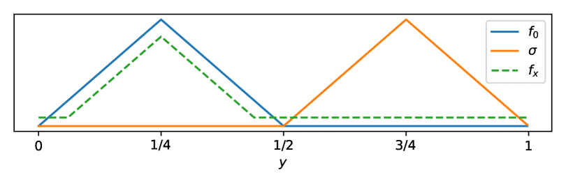
Figure 1: Illustration of the densities $\rho_{0}$ and $\rho_{x}$ for $x$ small, and the function $\sigma_{\text{SF}}\big{(}0,\cdot\big{)}$.

B.2.3 A Positive Result

We have just seen a counterexample where the square root of $\overline{A}$ is not Lipschitz continuous at zero, due to a specific configuration of the supports of $\rho_{0}$ and $\sigma_{\text{SF}}$. Now, we prove the following:

Lemma 13.

Assume that $\rho_{x}\big{(}y\big{)}\geq\delta>0$ for all $(x,y)\in\mathbb{X}\times\mathbb{T}$. Then $\psi\big{(}x\big{)}:=\sqrt{\overline{A}\big{(}x\big{)}}$ is Lipschitz continuous in $x$.

Proof.

We write

$$\psi\big{(}x+h\big{)}-\psi\big{(}x\big{)}=\frac{\overline{A}\big{(}x+h\big{)}-\overline{A}\big{(}x\big{)}}{\psi\big{(}x+h\big{)}+\psi\big{(}x\big{)}}.$$

Let us analyze the numerator. We decompose it into two terms:

$$\overline{A}\big{(}x+h\big{)}-\overline{A}\big{(}x\big{)}=\int_{0}^{1}\sigma_{\text{SF}}\big{(}x+h,y\big{)}^{2}\bigg{(}\rho_{x+h}\big{(}y\big{)}-\rho_{x}\big{(}y\big{)}\bigg{)}dy+\int_{0}^{1}\bigg{(}\sigma_{\text{SF}}\big{(}x+h,y\big{)}^{2}-\sigma_{\text{SF}}\big{(}x,y\big{)}^{2}\bigg{)}\rho_{x}\big{(}y\big{)}dy.$$

Because $\rho$ is $l$-Lipschitz in $x$, the absolute value of the first term is bounded by:

$$\Bigg{|}\int_{0}^{1}\sigma_{\text{SF}}\big{(}x+h,y\big{)}^{2}\bigg{(}\rho_{x+h}\big{(}y\big{)}-\rho_{x}\big{(}y\big{)}\bigg{)}dy\Bigg{|}\leqslant\Bigg{(}\int_{0}^{1}\sigma_{\text{SF}}\big{(}x+h,y\big{)}^{2}dy\Bigg{)}l|h|$$

For the second term, we rewrite the integrand using $a^{2}-b^{2}=(a-b)(a+b)$ and apply the Lipschitz continuity of $\sigma_{\text{SF}}$:

$$\Bigg{|}\int_{0}^{1}\bigg{(}\sigma_{\text{SF}}\big{(}x+h,y\big{)}^{2}-\sigma_{\text{SF}}\big{(}x,y\big{)}^{2}\bigg{)}\rho_{x}\big{(}y\big{)}dy\Bigg{|}\leqslant\Bigg{(}\int_{0}^{1}\bigg{|}\sigma_{\text{SF}}\big{(}x+h,y\big{)}+\sigma_{\text{SF}}\big{(}x,y\big{)}\bigg{|}\rho_{x}\big{(}y\big{)}dy\Bigg{)}M|h|.$$

Note that we may assume $\sigma_{\text{SF}}$ is non-negative, as this does not affect its Lipschitz constant. Similarly, we take the positive square root of $\overline{A}$ to define $\psi$.

It thus suffices to find constants $C_{1}$ and $C_{2}$ such that:

$$\frac{1}{\psi\big{(}x+h\big{)}}\int_{0}^{1}\sigma_{\text{SF}}\big{(}x+h,y\big{)}^{2}dy\leq C_{1}\quad\text{and}\quad\frac{1}{\psi\big{(}x\big{)}}\int_{0}^{1}\sigma_{\text{SF}}\big{(}x,y\big{)}\rho_{x}\big{(}y\big{)}dy\leq C_{2}.$$

The first inequality follows from the fact that $\rho$ is bounded below by $\delta$. Indeed, the denominator is at least:

$$\delta\sqrt{\int_{0}^{1}\sigma_{\text{SF}}\big{(}x+h,y\big{)}^{2}dy},$$

so it suffices to choose:

$$C_{1}\geq\frac{1}{\delta}\sqrt{\int_{0}^{1}\sigma_{\text{SF}}\big{(}x+h,y\big{)}^{2}dy}$$

Since $\sigma_{\text{SF}}$ is continuous (and therefore bounded), the integral above is uniformly bounded.

For the second term, we apply the Cauchy–Schwarz inequality to the pair $\sigma_{\text{SF}}\big{(}x,y\big{)}\sqrt{\rho_{x}\big{(}y\big{)}}$ and $\sqrt{\rho_{x}\big{(}y\big{)}}$, since

$$\int_{0}^{1}\rho_{x}\big{(}y\big{)}dy=1.$$

∎

References

• [AB01] Olivier Alvarez and Martino Bardi. Viscosity solutions methods for singular perturbations in deterministic and stochastic control. SIAM J.Control Optim, 40:1159–1188, 2001.
• [AB03] Olivier Alvarez and Martino Bardi. Singular perturbations of nonlinear degenerate parabolic pdes: a general convergence result. Ration. Mech. Anal, 170:17–61, 2003.
• [AB10] Olivier Alvarez and Martino Bardi. Ergodicity, Stabilization, and Singular Perturbations for Bellman-Isaacs Equations. American Mathematical Society, 1º edition, 2010.
• [ABG12] Ari Arapostathis, Vivek S. Borkar, and Mrinalk. Ghosh. Encyclopedia of Mathematics and Its Applications: ergodic control of diffusion processes. Springer, 1º edition, 2012.
• [ABM07] Olivier Alvarez, Martino Bardi, and Claudio Marchi. Multiscale problems and homogenization for second-order hamilton–jacobi equations. J.Differential Equations, 2007.
• [BC09] Martino Bardi and Annalisa Cesaroni. Optimal control with random parameters: a multiscale approach. European Journal of Control, 17:30–45, 2009.
• [BCD97] Martino Bardi and Italo Capuzzo-Dolcetta. Optimal Control and Viscosity Solutions of Hamilton-Jacobi-Bellman Equations. Birkhauser, 1º edition, 1997.
• [BCM10] Martino Bardi, Annalisa Cesaroni, and Luigi Manca. Convergence by viscosity methods in multiscale financial models with stochastic volatility. SIAM J.Financial Math, 1:230–265, 2010.
• [Ber18] Dimitri P. Bertsekas. Abstract Dynamic Programming. Athena Scientific, 1º edition, 2018.
• [BKR01] Vladimir I. Bogachev, Nicolai V. Krylov, and Michael Röckner. On regularity of transition probabilities and invariant measures of singular diffusions under minimal conditions. Communications in Partial Differential Equations, 26:11–12, 2001.
• [BKRS15] Vladimir I. Bogachev, Nicolai V. Krylov, Michael Röckner, and Stanislav V. Shaposhnikov. Fokker–Planck–Kolmogorov Equations. American Mathematical Society, 1º edition, 2015.
• [BL14] Johann Baumeister and Antonio Leitão. Introdução a Teoria do Controle Ótimo e da Programação Dinâmica. IMPA, 1º edition, 2014.
• [CD99] Doina Cioranescu and Patrizia Donato. An Introduction to Homogenization. Oxford University Press, 1º edition, 1999.
• [CIL92] Michael G. Crandall, Hitoshi Ishii, and Pierre-Louis Lions. Users guide to viscosity solutions of second order partial differential equations. Appeared in Bulletin of the American Mathematical Society, 27:1–67, 1992.
• [Eva10] Lawrence C. Evans. Partial Differential Equations. American Mathematical Society, 2º edition, 2010.
• [FR86] Wendell H. Fleming and Raymond W. Rishel. Deterministic and Stochastic Optimal Control. Springer, 3º edition, 1986.
• [FS06] Wendell H. Fleming and H. Mete Soner. Controlled Markov Processes and Viscosity Solutions. Springer, 2º edition, 2006.
• [Gal14] Jean-François Le Gall. Brownian Motion, Martingales, and Stochastic Calculus. Springer, 1º edition, 2014.
• [IKO02] A. M. Ilyin, A. S. Kalashnikov, and O. A. Oleynik. Linear second order partial differential equations of the parabolic type. Journal of Mathematical Sciences, 108, 2002.
• [KD01] Harold J. Kushner and Paul Dupuis. Numerical Methods for Stochastic Control Problems in Continuous Time. Springer, 2º edition, 2001.
• [Kha11] Rafail Khasminskii. Stochastic Stability of Differential Equations. Springer, 2º edition, 2011.
• [Koc15] Mykel J. Kochenderfer. Decision Making Under Uncertainty: theory and applications. MIT Press, 1º edition, 2015.
• [KRS08] Nicolai V. Krylov, Michael Röckner, and Stanislav V. Shaposhnikov. Lectures on Elliptic and Parabolic Equations in Sobolev Spaces. American Mathematical Society, 1º edition, 2008.
• [Kus90] Harold J. Kushner. Weak Convergence Methods and Singularly Perturbed Stochastic Control and Filtering Problems. Birkhauser, 1º edition, 1990.
• [LH18] Luciano Losekann and Michelle Hallack. Novas Energias Renováveis no Brasil: desafios e oportunidades. Instituto de Pesquisa Econômica Aplicada, 2018.
• [LS84] P. L. Lions and A. S. Sznitman. Stochastic differential equations with reflecting boundary conditions. Communications on Pure and Applied Mathematics, XXXVII, 1984.
• [Oks00] Bernt Oksendal. Stochastic Differential Equations. Springer, 5º edition, 2000.
• [ONS23] Plano da Operação Energética 2023/2027 PEN 2023. Operador Nacional do Sistema Elétrico, 2023.
• [Pav14] Grigorios A. Pavliotis. Stochastic Processes and Applications: diffusion processes, the Fokker-Planck and Langevin equations. Springer, 1º edition, 2014.
• [Pha09] Huyên Pham. Continuous Time Stochastic Control and Optimization with Financial Applications. Springer, 1º edition, 2009.
• [PIL09] Giovanni Parmigiani, Lurdes Y. T. Inoue, and Hedibert F. Lopes. Decision Theory: principles and approaches. Wiley, 1º edition, 2009.
• [Pil14] Andrey Pilipenko. An Introduction to Stochastic Differential Equations with Reflection. Potsdam University Press, 1º edition, 2014.
• [Pow11] Warren B. Powell. Approximate Dynamic Programming: solving the curses of dimensionality. Wiley, 2º edition, 2011.
• [PR14] Etienne Pardoux and Aurel Rascanu. Stochastic Differential Equations, Backward SDEs, Partial Differential Equations. Springer, 1º edition, 2014.
• [PS08] Grigorios A. Pavliotis and Andrew M. Stuart. Multiscale Methods: averaging and homogenization. Springer, 1º edition, 2008.
• [RRO22] Xavier Fernandez Real and Xavier Ros-Oton. Regularity Theory for Elliptic PDE. EMS Press, 1º edition, 2022.
• [Sal08] Sandro Salsa. Partial Differential Equations in Action: from modelling to theory. Prentice-Hall, 1º edition, 2008.
• [YZ99] Jiongmin Yong and Xun Yu Zhou. Stochastic Controls: hamiltonian systems and HJB equations. Springer, 1º edition, 1999.