Green Hacks: Generating Sustainability-Targeting Attacks For Cyber-Physical Systems

Abstract

Sustainability-targeting attacks (STA) or “Green Hacks” are a growing threat to cyber-physical system (CPS)-based infrastructure, as its performance objectives are increasingly linked to sustainability goals. These attacks exploit the interdependence between control, energy efficiency, and environmental impact to degrade systems’ overall performance. Thus, in this work, we propose a general mathematical framework for modeling such STA and derive the feasibility conditions for generating a worst-case STA on a linear CPS using a max-min formulation. A gradient ascent descent algorithm is used to construct the worst-case attack policy. We simulated the worst-case STA for a linear CPS to illustrate its impacts on the CPS performance and sustainability cost.

1 Introduction

As CPS-based critical infrastructure systems increasingly consume an enormous amount of energy, heavily interact with the environment, and focus on sustainability goals and regulatory restrictions, cyberattacks on these systems can directly impact the overall sustainability objectives. In particular, an adversary can specifically target these sustainability goals instead of disrupting system operations solely through conventional cyberthreats such as denial-of-service (DoS), replay attack, false-data injection, and so on. These emerging threats of sustainability-targeting attacks (STA) or “Green Hacks” on CPS motivate our interest in developing a general framework and analyzing their potential risks.

For the past decade, research has been primarily focused on the impact of cyberattacks on the output or the system performance of CPS [1, 2, 3, 4]. However, recently the focus has been extended to include STA in several CPS systems, including intelligent buildings, smart grids, data centers, and IoT systems. Among them, a major focus has been given to energy efficiency as a sustainability criterion. For instance, manipulation of demand via Internet of Things (IoT) attacks has been explored in [5], where attackers can control high-wattage devices to change the grid demand. Similarly, [6] introduced malicious energy attacks in green IoT networks, where attackers used reinforcement learning techniques like Q-learning and Policy Gradient to change specific network nodes to redirect the traffic through compromised nodes effectively. In [7], the authors explored the energy depletion of IoT device batteries by using diffusion approximation and examined the impacts of ghost energy depletion attacks on device lifetime. Moreover, [8] analyzed the effects of DoS attacks on energy consumption and CPU usage of IoT devices and used a testbed platform to observe the impact of synchronization flood attack and Internet Control Message Protocol flood attack on device performance. In [9], a smart energy theft system (SETS) that uses machine learning models to identify fraudulent power consumption in IoT-enabled smart homes is introduced. The worst-case power injection attacks on smart distribution grids are discussed in [10], where the authors identified the system vulnerabilities and suggested grid design optimization and grid reconfiguration algorithms to reduce the impact of these attacks. Moreover, [11] explored the use of a novel side-channel by attackers in multi-tenant data centers to monitor power consumption and execute power attacks.

Apart from energy sustainability criteria, several works also included other sustainability factors, such as operational/economic cost, system longevity, and ecological impact. [12] used dynamic co-simulator models to assess how cyberattacks on smart grids can cause economic losses and threaten the sustainable operation by undermining the critical infrastructure of power systems. Similarly, the authors in [13] highlighted how the communication protocols, data integrity, and control commands of the smart grid can be exploited to launch DoS and false data infection attacks and emphasized the need for security against cyberattacks in the smart grid to prevent economic disruption and protect the power infrastructure. Researchers have also evaluated smart electrical meters under SYN (synchronize) flood and network congestion attacks and have shown that these can cause delays and data corruption during energy reporting, leading to revenue loss for utility companies [14]. In addition, [15] simulated DoS and Man-in-the-Middle attacks on connected and Automated vehicles (CAVs), and showed that compromised roadside Units (RSUs) can lead to communication failures and an increase in travel delays by over 20% per vehicle. Another study [16] evaluated how sensor spoofing and communication jamming cyberattacks can increase up to 14% more energy consumption in low-level automated vehicles by disrupting their longitudinal trajectory. Similarly, [17] analyzed a real-world supervisory control and data acquisition (SCADA) cyberattack on the water infrastructure, where an insider exploited vulnerable wireless access to release raw sewage in the environment that disrupted services and polluted ecosystems.

In addition to STA policy generation, research has also been focused on detecting STA in CPS. For example, [18] proposes an entropy-based detection method for DoS attacks using virtual machine status patterns. Since low-powered IoT devices are vulnerable to information leakage and energy drain attacks, the authors in [19] introduced a detection algorithm and compared the energy consumption differences with and without such STA attacks. Furthermore, [20] proposed an optimal strategic threshold value through Nash equilibrium for blocking economic denial of sustainability attacks in cloud computing. While [21] proposed a defense system against economic denial of sustainability attacks using source checking, counting, and Turing tests, [22] adopted an efficient client-puzzle approach. Similarly, in [23], the authors discussed power attacks on data centers that can cause undesired power outages and provided mitigation approaches for maintaining power usage sustainability goals. Additionally, a cost-effective Power Attack Defense system is proposed in [24] to counter the Power Virus attacks on data centers. Another study [25] proposed a Transient System Simulation Tool model of a 12-zone HVAC system (a data-driven attack detection strategy with lower computational cost) to enhance security against cyberattacks on HVAC systems in smart buildings, preventing STA and increasing the power efficiency of smart buildings.

However, a general framework for cyberattacks that target the sustainability goals of a CPS has remained unexplored to the best of our knowledge. Additionally, under this general framework, there exists a crucial research gap in formulating and analyzing the feasibility of the worst-case STA for risk assessment in sustainability-focused CPS. To address these research gaps, our particular contributions in this work are:

1. formulating a general framework for STA for a linear sustainable CPS,

2. feasibility analysis for the worst-case STA generation,

3. implementation of a Gradient Ascent Descent (GAD) algorithm to construct the worst-case STA policy.

The organization of this paper is as follows: Section 2 presents a susceptibility-targeting attack model. Section 3 presents the feasibility analysis and policy generation algorithm using GAD. Section 4 presents the simulation results for linear CPS with a quadratic cost for sustainability. We finally summarize our work in Section 5.

Notations: This paper uses $\mathbb{R}^{a}$ as a $a$-dimensional Euclidean space. The 2-norm (also called the Euclidean norm) of a vector is $\|x\|:=(x^{T}x)^{1/2}$. The scalar product of two $p$-dimensional vectors is defined as $\big{(}x,y\big{)}:=\sum_{p=1}^{r}x_{p}^{T}y_{p}$. $C(I)$ is the space of continuous functions that change smoothly over an interval $I$. $L^{1}(I)$ is the space of Lebesgue integrable functions over a finite interval $I$. If $f\in L^{1}(I)$ then the $L^{1}$ norm of $f$ i.e. $\int_{I}|f(t)|\,dt<\infty$.

2 Modeling Framework for STA

A security framework for CPS is divided into the administrator space and the adversarial space. The administrator space for CPS consists of the plant, a central controller, and a closed communication network connecting the plant and the controller. The CPS output is measured and sent via the cloud to a central controller that implements specific control policies to obtain a control input $u$. In a sustainable CPS plant, this controller objective consists of both operational and sustainability goals. The latter is often satisfied by the administrator by minimizing a sustainability cost through an optimal control input $u$. In contrast, in the adversarial space, all or partial system information and measurements are used to craft cyberattacks to fulfill the goals of the adversary. Particularly, for an attack that aims to disrupt the sustainability goals of the administrator, aka STA $\delta$, the adversary aims to maximize the sustainability cost $\mathcal{J}$ through the corruption of control input $u$. Fig. 1 shows the schematic of the different components of the CPS administrator space and the adversarial space generating the STA to corrupt control input $u$ through cloud communication.

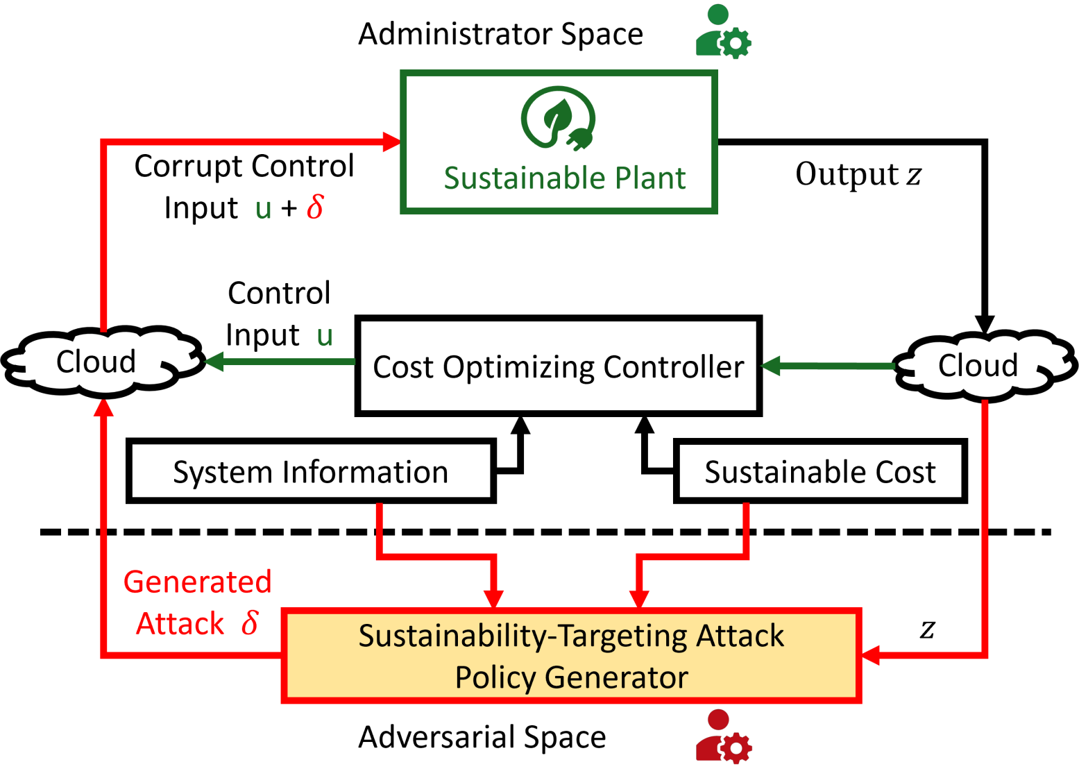
Figure 1: A schematic of the administrative and adversarial space in the context of sustainability-targeting attacks on CPS.

To present the mathematical framework for STA, we will first represent a linear CPS that is under an attack that corrupts the control input:

$$\dot{x} =\mathcal{A}x+\mathcal{B}u,$$ (1)

$$u =-\mathcal{K}z+\delta,\quad z=\mathcal{L}x,$$ (2)

where $x\in\mathbb{R}^{i}$ is a state vector, $u\in\mathcal{N}_{u}\in\mathbb{R}^{k}$ is the control input, and $z\in\mathbb{R}^{j}$ denotes the measured output. The attack generated by the adversary is denoted by $\delta$ such that it belongs to the set of all possible attacks $\mathcal{N}_{d}\subset\mathbb{R}^{k}$, and the control input $u$ belongs to the admissible set $\mathcal{N}_{u}$. In addition, $\mathcal{A}\in\mathbb{R}^{i\times i},\mathcal{B}\in\mathbb{R}^{i\times k}$, $\mathcal{L}\in\mathbb{R}^{j\times i}$, and $\mathcal{K}\in\mathbb{R}^{k\times j}$ are the state, input, observation, and feedback gain matrices, respectively. Now, let the sustainability cost function over the time interval $I=[0,T]$ be given by

$$\mathcal{J}(u,\delta):=\int_{I}w(t,x)dt+\theta(x(T)).$$ (3)

where $w(t,x(t))$ is the running cost and $\theta(x(t))$ is the terminal cost for the system (1)-(2). For instance, the sustainability cost function can capture the loss in building energy utilization [26] or the marginal emission factor for electric vehicles [27]. The goal of the defender here is to minimize this sustainability cost (3) of the CPS (e.g., minimize energy loss in buildings or emissions in electric vehicles) with the least control action $u$ (2). On the other hand, the attacker attempts to maximize the sustainability cost (3) by designing $\delta$. Thus, the defender seeks an optimal control policy $u_{0}$ that minimizes $\mathcal{J}$, while the attacker simultaneously attempts to design a worst-case STA policy $\delta_{0}$ that maximizes $\mathcal{J}$ to specifically target sustainability goals. In the framework of dynamic games, this worst-case STA policy can be obtained by the attacker by solving the following max-min problem, subject to the dynamics of the CPS (1)-(2) is given by $\max_{\delta\in\mathcal{N}_{d}}\min_{u\in\mathcal{N}_{u}}\mathcal{J}(u,\delta).$ While the cost function of the system is minimized with respect to the control input $u$, we can reformulate this optimization in terms of the feedback gain $\mathcal{K}$ by substituting the control input (2) to obtain

$$\max_{\delta\in\mathcal{N}_{d}}\min_{\mathcal{K}\in\mathcal{N}_{\mathcal{K}}}\mathcal{J}(\mathcal{K},\delta),$$ (4)

where the feedback gain $\mathcal{K}$ belongs to the admissible set of the feedback gain values of $\mathcal{N}_{\mathcal{K}}\subset\mathbb{R}^{k\times j}$.

3 Feasibility Analysis And Policy Generation

In this section, we will show the feasibility of solving the max-min problem (4) under the constraint of the CPS dynamics (1)-(2) to obtain the worst-case STA policy. The feasibility analysis will also enable us to propose an algorithm for generating the STA using a GAD strategy.

3.1 Feasibility of worst-case STA

To derive the conditions that guarantee the feasibility of the worst-case STA for a linear CPS, we consider the following assumptions about the access to system information by the attacker and the regularity of the cost functions and the convexity of admissible sets for $u$ and $\delta$.

Assumption 1 (Attacker knowledge).

Attackers have complete information of the CPS, i.e., knowledge of $\mathcal{A},\mathcal{B},\mathcal{L}$ and the sustainability cost $\mathcal{J}$ to obtain a specific sustainability goal. The attacker has full access to the actuator and can modify $u$ to $u+\delta$.

Remark 1.

While complete knowledge of the system can be unrealistic in a practical setting, analyzing the worst-case attack under this assumption is critical. Several attack scenarios, such as stealthy attack, byzantine attack, white-box attacks, or man-in-the-middle attacks, are often analyzed under the assumption of full-system knowledge [28] and show the fundamental threats in the system design.

Assumption 2 (Bounded control input $u$ and bounded attack $\delta$).

The control input $u(t)\in C(I)$ and is bounded. This implies that $u(t)\in L^{1}(I),$ where $L^{1}(I)$ is a Hilbert space. The attack $\delta(t)\in C(I)$ and is bounded i.e. $\delta(t)\in L^{1}(I).$

Assumption 3 (Convexity of feasible attack set).

The set of all admissible attacks $\mathcal{N}_{d}$ is a convex set. This implies that for any $\epsilon\in[0,1]$ and any two attacks $\delta_{1},\delta_{2}\in\mathcal{N}_{d}$, the convex combination $\delta_{\epsilon}=\epsilon\delta_{1}+(1-\epsilon)\delta_{2}\in\mathcal{N}_{d}$.

Assumption 4 (Regularity of cost function and trajectory).

The running cost $w(t,x)$ and the terminal cost $\theta(x)$ are continuously differentiable with respect to the state $x$ and are bounded, such that the accumulated cost $\forall t\in I$ is finite. Additionally, we assume that the state trajectory $x(t)$ is $C(I)$.

We derive the closed-loop system of (1)-(2) by substituting $z$ to get $u=-\mathcal{K}\mathcal{L}x+\delta$, which changes (1) to:

$$\dot{x}=\mathcal{A}x-\mathcal{B}\mathcal{K}\mathcal{L}x+\mathcal{B}\delta.$$ (5)

We will apply a variational approach to determine the worst-case STA $\delta_{0}$ in the presence of an optimal control gain $\mathcal{K}_{0}$. Thus, we define a Hamiltonian function using (3) and (5)

$$\mathcal{H}(t,x,\Omega,\delta):= (\mathcal{A}x-\mathcal{B}\mathcal{K}_{0}\mathcal{L}x+\mathcal{B}\delta,\Omega)+w(t,x).$$ (6)

Our goal here is to show that the necessary conditions for deriving the worst-case STA are equivalent to maximizing the Hamiltonian $\mathcal{H}$. The costate variable $\Omega$ in (6) captures the cost of violating the system dynamics during optimization. Inspired by [29], we prove our main theorem to derive the feasibility conditions for the worst-case STA $\delta_{0}$.

Theorem 1 (Existence of STA attacks).

Let us consider the closed-loop linear CPS system (5) with sustainability cost (3) where Assumptions  1-  4 are valid. Under these assumptions, for an optimal controller gain $\mathcal{K}_{0}$ that minimizes the cost, an STA attack $\delta_{0}$ exists in the sense of the max-min problem (4) and produces a state trajectory $x_{0}$ and a costate trajectory $\Omega_{0}$, if the following three conditions are satisfied for $\forall t\in I$:

1. $$\mathcal{H}(t,x_{0}(t),\Omega_{0}(t),\delta_{0}(t))\!\geqslant\!\mathcal{H}(t,x_{0}(t),\Omega_{0}(t),\delta(t)),$$ (7)

2. $$\dot{x}_{0}=\mathcal{H}_{\Omega}(t,x_{0},\Omega_{0},\delta_{0}),\quad x_{0}(0)=\upsilon,$$ (8)

3. $$\dot{\Omega}_{0}=-\mathcal{H}_{x}(t,x_{0},\Omega_{0},\delta_{0}),\,\Omega_{0}(T)=\theta_{x}(x_{0}(T)).$$ (9)

Proof.

Let us consider an optimal feedback control gain $\mathcal{K}_{0}\in\mathcal{N}_{\mathcal{K}}$ and the corresponding sustainability cost

$$\mathcal{J}(\mathcal{K}_{0},\delta_{0}):=\int_{I}w(t,x_{0}(t))dt+\theta(x_{0}(T)),$$ (10)

where the state $x_{0}(t):=x(t,\mathcal{K}_{0},\delta_{0})$ is the solution of

$$\dot{x}_{0}=\mathcal{A}x_{0}-\mathcal{B}\mathcal{K}_{0}\mathcal{L}x_{0}+\mathcal{B}\delta_{0},\ x_{0}(0)=\upsilon,\,t\in I.$$ (11)

Now, we suppose that $\delta_{0}\in\mathcal{N}_{d}$ is the worst-case attack for the optimal gain $\mathcal{K}_{0}$ and $\delta\in\mathcal{N}_{d}$ is any other attack. Since $\mathcal{N}_{d}$ is a closed convex set, for any $\epsilon\in(0,1)$ the combination of $\delta$ and $\delta_{0}$ such as $\delta_{\epsilon}:=\delta_{0}+\epsilon(\delta-\delta_{0})$ is also in the admissible set $\mathcal{N}_{d}$. This perturbed attack $\delta_{\epsilon}$ helps us examine how the cost functional changes when we change the STA attack $\delta_{0}$ subtly. Now, the solution of (11) corresponding to the perturbed attack $\delta_{\epsilon}$ is denoted as $x_{\epsilon}$. Since $\delta_{0}$ is the maximum attack, we have $\mathcal{J}(\mathcal{K}_{0},\delta_{0})\geqslant\mathcal{J}(\mathcal{K}_{0},\delta_{\epsilon})$, $\forall\epsilon\in(0,1)$. Next, dividing the inequality by $\epsilon$ and using (3) we obtain: $\frac{1}{\epsilon}\left(\mathcal{J}(\mathcal{K}_{0},\delta_{\epsilon})-\mathcal{J}(\mathcal{K}_{0},\delta_{0})\right)=\frac{1}{\epsilon}\left[\int_{I}(w(t,x_{\epsilon}(t))-w(t,x_{0}(t)))\,dt+\theta(x_{\epsilon}(T))-\theta(x_{0}(T))\right]$ $\leqslant 0.$ As $\epsilon\to 0$, this yields the Gateaux derivative $d\mathcal{J}(\mathcal{K}_{0},\delta_{0})$ of the cost functional $\mathcal{J}$ at $\delta_{0}$ and is given by

$$d\mathcal{J}(\mathcal{K}_{0},\delta_{0})=\mathbb{K}_{y}[J]\leqslant 0,\text{ where }$$ (12)

$$\mathbb{K}_{y}[J]:=\!\!\!\int_{I}\!\!\!\Big{(}w_{x}(t,x_{0}(t)),y(t)\Big{)}\,dt+\Big{(}\theta_{x}(x_{0}(T)),y(T)\Big{)},$$ (13)

and $y(t):=\lim_{\epsilon\to 0}\frac{x_{\epsilon}(t)-x_{0}(t)}{\epsilon}.$ Since by Assumption 4 $x,x_{\epsilon}\in C(I)$, then $y(t)\in C(I)$ is the solution of

$$\dot{y}=\mathcal{A}y-(\mathcal{B}\mathcal{K}_{0}\mathcal{L})y+\mathcal{B}(\delta-\delta_{0}),\quad y(0)=0.$$ (14)

This variational equation (14) shows how the perturbation $y(t)$ in the state evolves with a small variation in the attack $\delta_{0}$. Since the initial conditions $x_{0}(0)=x_{\epsilon}(0)=\nu$ are fixed of variations in the attack term, the state variation is $y(0)=0$. By Assumption 2 the attack $\delta,\delta_{0}\in L^{1}(I)$ is a bounded function and thus the driving term in (14), $\mathcal{B}(\delta-\delta_{0})\in L^{1}(I)$. This guarantees the existence and uniqueness of the solution $y\in C(I)$. Additionally, this implies that there exists a continuous map

$$\mathcal{B}(\delta-\delta_{0})\to y.$$ (15)

Next, from Assumption 4, the two terms $\int_{I}\big{(}w_{x}(t,x_{0}(t)\big{)}dt$ and $\theta_{x}\big{(}x_{0}(T)\big{)}$ are continuously differentiable with respect to $x$. Therefore, the map $y\to\mathbb{K}_{y}[J]$ is also continuous. Therefore, the composition of the two maps also yields a continuous linear mapping

$$\mathcal{B}(\delta-\delta_{0})\to\mathbb{K}_{y}[J].$$ (16)

Thus, (12) and (16) imply that the Gateaux derivative $d\mathcal{J}$ is a continuous linear functional $f$ of $\mathcal{B}(\delta-\delta_{0})\in L^{1}(I)$. Therefore, we can now apply the Riesz representation theorem [30] that guarantees the existence of a unique function $\Omega_{0}\in L^{1}(I)$ such that the Gateaux derivative of the cost function can be expressed as an inner product with $\Omega_{0}$. Additionally, using (12) we can infer $\forall\delta\in\mathcal{N}_{d}$

$$d\mathcal{J}=f\left(\mathcal{B}(\delta-\delta_{0})\right)=\int_{I}\Big{(}\mathcal{B}(\delta-\delta_{0}),\Omega_{0}\Big{)}\,dt\leqslant 0$$ (17)

This $\Omega_{0}$ can in fact be defined as our costate from the Hamiltonian (6). Consequently, observing (6), we can add more terms to the inequality $\int_{I}\big{(}\mathcal{B}\delta,\Omega_{0}\big{)}dt\leqslant\int_{I}\big{(}\mathcal{B}\delta_{0},\Omega_{0}\big{)}dt$ to obtain $\int_{I}[\mathcal{H}(t,x_{0},\Omega_{0},\delta)-\mathcal{H}(t,x_{0},\Omega_{0},\delta_{0})]dt\leqslant 0.$ Since this inequality is true $\forall\delta\in\mathcal{N}_{d}$, for some $s\in I$ we define $\delta(t)=\delta_{0}(t),\forall t\in I\backslash(s-\omega,s+\omega)$ and $\delta(t)=\mathcal{D}\in\mathcal{N}_{d}$ otherwise. This spike variation choice of $\delta$, reduces the integral to $\int_{s-\omega}^{s+\omega}[\mathcal{H}(t,x_{0},\Omega_{0},\mathcal{D})-\mathcal{H}(t,x_{0},\Omega_{0},\delta_{0})]dt\leqslant 0$ [31]. We note here that that $\mathcal{H}$ is an $L^{1}(I)$ on a measurable set $(s-\omega,s+\omega)$. Hence, we can use the Lebesgue differential theorem [32] by dividing both side by $\omega$ and set $\omega\to 0$, to obtain the point-wise inequality $\mathcal{H}(t,x_{0},\Omega_{0},\delta-\mathcal{H}(t,x_{0},\Omega_{0},\delta_{0}\leqslant 0,$ for almost all $t\in I$ and any $\delta\in\mathcal{N}_{d}.$ This proves condition (7).

Next, to prove the condition (8), we differentiate the Hamiltonian (6) with respect to the costate variable $\Omega$. This produces the right-hand side of the system dynamics expressed in (11) and we recover condition (8)

Subsequently, to prove the condition (9), we will first derive the costate dynamics. To achieve this, we will rearrange the terms in (14) to isolate $\mathcal{B}(\delta-\delta_{0})$ and substitute into (17)

$$d\mathcal{J}=\int_{I}\Big{(}\dot{y}-[\mathcal{A}y-(\mathcal{B}\mathcal{K}_{0}\mathcal{L})y],\Omega_{0}\Big{)}\,dt.$$ (18)

We apply integration by parts to the right side of (18) with $y(0)=0$ to obtain $\int_{I}\big{(}\dot{y}-[\mathcal{A}y-(\mathcal{B}\mathcal{K}_{0}\mathcal{L})y],\Omega_{0}\big{)}\,dt=\big{(}y(T),\Omega_{0}(T))-\int_{I}\big{(}y,\dot{\Omega}_{0}+\mathcal{A}^{T}\Omega_{0}-(\mathcal{B}\mathcal{K}_{0}\mathcal{L})^{T}\Omega_{0}\big{)}\,dt.$ Replacing this in (18), then using (12)-(13) and comparing, we obtain the costate dynamics:

$$\dot{\Omega}_{0}+\mathcal{A}^{T}\Omega_{0}-(\mathcal{B}\mathcal{K}_{0}\mathcal{L})^{T}\Omega_{0}=-w_{x}(t,x_{0}(t)),$$ (19)

with the terminal condition

$$\Omega_{0}(T)=\theta_{x}(x_{0}(T)).$$ (20)

Now, if we differentiate the Hamiltonian (6) with respect to the state variable $x$, we obtain the right-hand side of (19). This yields the third condition specified in (9) and completes the proof.

∎

With the derivation of the necessary conditions for the existence of the worst-case STA $\delta_{0}$ in Theorem 1, we will present an algorithmic approach to construct it.

3.2 Gradient ascent-descent (GAD) algorithm for the worst-case STA generation

In this section, we describe a GAD algorithm [33] that is used to obtain the worst-case STA policy for our linear dynamical system (1)-(2). Here, the gradient descent method is followed by the gradient ascent to calculate the optimal feedback gain $\mathcal{K}_{0}$ and the worst-case STA $\delta_{0}$, respectively. During the gradient descent step, we update the feedback control gain $\mathcal{K}$ by using the gradient descent equation

$$\mathcal{K}^{l+1}=\mathcal{K}^{l}-\alpha_{\mathcal{K}}\nabla_{\mathcal{K}}\mathcal{H},$$ (21)

to find the optimal value of feedback control gain $\mathcal{K}$ for which the cost function is minimum. Similarly, in the gradient ascent step, the value of the attack $\delta$ is updated progressively to find the worst-case STA by maximizing the cost function via

$$\delta^{l+1}=\delta^{l}+\alpha_{\delta}\nabla_{\delta}\mathcal{H}.$$ (22)

Here, $\alpha_{\mathcal{K}}$, $\alpha_{\delta}>0$ are respectively the learning rates for the ascent and descent parts. $\mathcal{K}^{l}$ and $\delta^{l}$ are the gain and attack in the $l^{th}$ iteration.

The algorithm begins with the initial states of the system and initial guesses for the feedback gain and attack from their respective feasible sets. Now, the adjoint state $\Omega$ is computed by solving the costate equation (9) over the whole time window. Then we will evaluate $\nabla_{\mathcal{K}}\mathcal{H}$ using (6) and obtain the updated feedback gain from (21). With this updated control gain and costate variable, we compute $\nabla_{\delta}\mathcal{H}^{l}$ from (6) and obtain the updated STA policy $\delta^{l+1}$ from (22). The stopping criterion for this algorithm is set until the change in cost function (10) between successive iterations is less than a set tolerance $\eta$. The details of this GAD-based STA generation method have been presented in Algorithm 1.

1

Input: Number of GAD iterations $N$, initial guesses for gain $\mathcal{K}^{1}$ and attack $\delta^{1}$, learning rates $\alpha_{\mathcal{K}},\alpha_{\delta}$, tolerance $\eta$.

2

Output: Optimal gain $\mathcal{K}_{0}$, Worst-case attack $\delta_{0}$

3

4$x^{1}(t),\mathcal{J}^{1}\,\leftarrow$ Cost_Fn($\mathcal{K}^{1},\delta^{1}$)

5 for $l=1:N$ do

6    $\Omega^{l}(t),\mathcal{K}^{l+1}\leftarrow$ Grad_Desc($x^{l}(t),\mathcal{K}^{l},\delta^{l}$)

7   

8   $\delta^{l+1}\leftarrow$ Grad_Asc($x^{l}(t),\mathcal{K}^{l+1},\delta^{l},\Omega^{l}(t)$)

9   

10   $x^{l+1}(t),\mathcal{J}^{l+1}\,\leftarrow$ Cost_Fn($\mathcal{K}^{l+1},\delta^{l+1}$)

11   

12   if $|\mathcal{J}^{l+1}-\mathcal{J}^{l}|<\eta$ then

13      

14       $\mathcal{K}_{0}\leftarrow\mathcal{K}^{l+1},\delta_{0}\leftarrow\delta^{l+1}(t)$

15       break

16   

17 function Cost_Fn($\mathcal{K}^{l},\delta^{l}$):

18    Compute $x^{l}(t),\forall t$ from (1); $\mathcal{J}^{l}$ from (10).

19    return $x^{l}(t),\mathcal{J}^{l}$ ;

20

21 function Grad_Desc($x^{l}(t),\mathcal{K}^{l},\delta^{1}$):

22    Compute $\Omega^{l}(t),\forall t$ from (9); $\nabla_{\mathcal{K}}\mathcal{H}^{l}$ from (6); $\mathcal{K}^{l+1}$ from (21).

23    return $\Omega^{l}(t),\mathcal{K}^{l+1}$ ;

24   

25

26 function Grad_Asc($x^{l}(t),\mathcal{K}^{l+1},\delta^{l},\Omega^{l}(t)$):

27    Compute $\nabla_{\delta}\mathcal{H}^{l}$ from (6); $\delta^{l+1}$ from (22)

28    return $\delta^{l+1}$;

29

Algorithm 1 Gradient Ascent Descent Algorithm

4 SIMULATION RESULTS

We will now present a simulation case study to show the efficacy of Algorithm 1 in generating the worst-case STA for a linear CPS. We also measure the impact of the worst-case attack $\delta_{0}$ on the sustainability performance of the system compared to a no-attack scenario $(\delta=0)$ with optimal sustainability performance. In this work, the linear system (1)-(2) has been chosen as $\mathcal{A}=[1\ 2;1\ 2]$, $\mathcal{B}=[2\ 1]^{T}$. This is a full-state feedback system, i.e. $y=x$, and our goal here is to reach the zero steady-state. To capture the performance and sustainability costs for this illustrative example, we have chosen an illustrative quadratic sustainability cost functional:

$$\mathcal{J}(u,\delta)=\int_{0}^{T}\big{(}\|x(t)\|^{2}+\|u(t)\|^{2}-\gamma\|\delta(t)\|^{2}\ \big{)}dt.$$ (23)

The term $\gamma\|\delta(t)\|^{2}$ represents the impact of the attack injected in the system on the sustainability cost $\mathcal{J}$ and is weighted by a regularization parameter $\gamma>0$. The negative sign with $\|\delta(t)\|^{2}$ in (23) implies that the attack causes an increase in the system’s sustainability cost. Similarly, the positive sign with the control input and state implies that less control energy and effective control both will decrease the sustainability cost. The time horizon is chosen to be $T=100s.$ The corresponding Hamiltonian for (23) can be defined as

$\mathcal{H}=\Omega^{T}[(A-BK)x+Bd]+\|x(t)\|^{2}+\|u(t)\|^{2}-\gamma\|\delta(t)\|^{2}$.

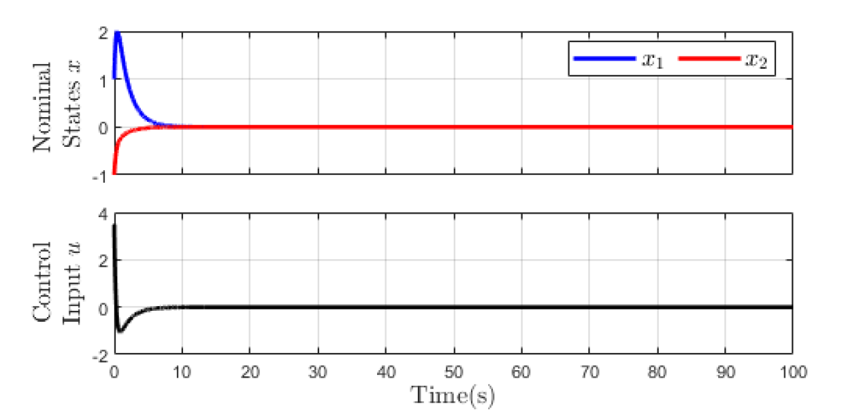
Figure 2: System under nominal conditions: top plot shows controlled system trajectories and bottom plot shows the LQR-based control input.

For this system, Figure 2 shows the performance for a nominal situation, under the Linear Quadratic Regulator (LQR) control gain [34] $\mathcal{K}=[1.26\ 4.76]$. The top plot of Figure 2 shows that the state trajectories are stabilized under no attack, and the total cost $\mathcal{J}=8.47$ is minimized. The LQR control input $u(t)$ also remains low throughout the time horizon and reaches $u=0$, as shown in the bottom plot of Figure 2. This confirms that the administrator achieves improved sustainability performance.

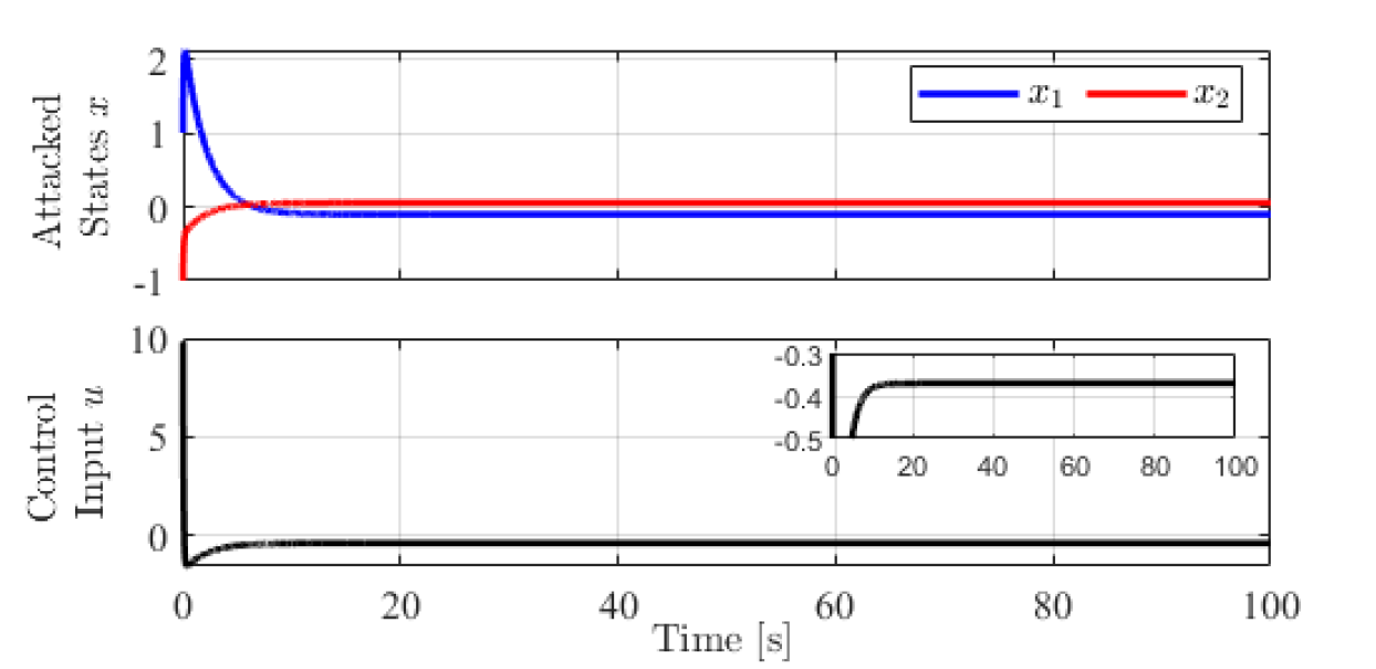
Figure 3: System performance under attack: top plot shows deviations from the reference trajectories and bottom plot shows nominal control input.

Next, we analyze how this system behaves when the defender tries to minimize the sustainability cost $\mathcal{J}$ while the attacker simultaneously tries to maximize it. Using Algorithm 1, the attacker generates the worst-case STA $\delta_{0}=0.37$. On the other hand, the administrator sets the optimal feedback gain as $\mathcal{K}_{0}=[2.74\ 12.55]$ to achieve the best-case control under attack, and the corresponding control input reaches $-0.37$, vide inset of the bottom plot of Figure 3. Under the worst-case attack, the system trajectories thus settle to $x=[-0.10\ 0.05]^{T}$, as shown in the top plot of Figure 3. The sustainability cost under the worst-case STA policy is given by $\mathcal{J}=10.12$, which is a 19.5% increase compared to the nominal operating condition.

5 CONCLUSIONS

In this work, we proposed a theoretical framework for modeling a cyberattack that can compromise the sustainability goals of an administrator using a min-max optimization. We have derived the necessary conditions for generating the worst-case STA policy using the Hamiltonian function and costate dynamics for a linear sustainable CPS. Additionally, we have provided an algorithmic strategy using gradient ascent and descent methods to construct the worst-case STA attacks. The algorithm is implemented for an illustrative example, and the simulation results show that the worst-case STA causes the states to deviate from the desired performance and contribute to higher control actions. Consequently, the total sustainability cost increased significantly for the worst-case attack policy, compared to the nominal scenario.

References

- [1] Seyed Mehran Dibaji, Mohammad Pirani, David Bezalel Flamholz, Anuradha M Annaswamy, Karl Henrik Johansson, and Aranya Chakrabortty. A systems and control perspective of cps security. Annual reviews in control, 47:394–411, 2019.
- [2] André Teixeira, Saurabh Amin, Henrik Sandberg, Karl H Johansson, and Shankar S Sastry. Cyber security analysis of state estimators in electric power systems. In 49th IEEE conference on decision and control (CDC), pages 5991–5998. IEEE, 2010.
- [3] Tanushree Roy and Satadru Dey. Actuator anomaly detection in linear parabolic distributed parameter cyber-physical systems. IEEE Transactions on Control Systems Technology, 2023.
- [4] Tanushree Roy and Satadru Dey. Secure traffic networks in smart cities: Analysis and design of cyber-attack detection algorithms. In 2020 American Control Conference (ACC), pages 4102–4107. IEEE, 2020.
- [5] Tohid Shekari, Celine Irvene, Alvaro A Cardenas, and Raheem Beyah. Mamiot: Manipulation of energy market leveraging high wattage iot botnets. In Proceedings of the 2021 ACM SIGSAC Conference on Computer and Communications Security, pages 1338–1356, 2021.
- [6] Long Li, Yu Luo, Jing Yang, and Lina Pu. Reinforcement learning enabled intelligent energy attack in green iot networks. IEEE Transactions on Information Forensics and Security, 17:644–658, 2022.
- [7] Godlove Suila Kuaban, Erol Gelenbe, Tadeusz Czachórski, Piotr Czekalski, and Julius Kewir Tangka. Modelling of the energy depletion process and battery depletion attacks for battery-powered internet of things (iot) devices. Sensors, 23(13):6183, 2023.
- [8] Buğra Kepçeoğlu, Azhar Murzaeva, and Sercan Demirci. Performing energy consuming attacks on iot devices. In 2019 27th Telecommunications Forum (TELFOR), pages 1–4. IEEE, 2019.
- [9] Weixian Li, Thillainathan Logenthiran, Van-Tung Phan, and Wai Lok Woo. A novel smart energy theft system (sets) for iot-based smart home. IEEE Internet of Things Journal, 6(3):5531–5539, 2019.
- [10] Martin Lindström, Hampei Sasahara, Xingkang He, Henrik Sandberg, and Karl Henrik Johansson. Power injection attacks in smart distribution grids with photovoltaics. In 2021 European Control Conference (ECC), pages 529–534. IEEE, 2021.
- [11] Mohammad A Islam and Shaolei Ren. Ohm’s law in data centers: A voltage side channel for timing power attacks. In Proceedings of the 2018 ACM SIGSAC Conference on Computer and Communications Security, pages 146–162, 2018.
- [12] Doney Abraham, Øyvind Toftegaard, Binu Ben Jose DR, Alemayehu Gebremedhin, and Sule Yildirim Yayilgan. Consequence simulation of cyber attacks on key smart grid business cases. Frontiers in Energy Research, 12:1395954, 2024.
- [13] Bishowjit Paul, Auvizit Sarker, Sarafat Hussain Abhi, Sajal Kumar Das, Md Firoj Ali, Md Manirul Islam, Md Robiul Islam, Sumaya Ishrat Moyeen, Md Faisal Rahman Badal, Md Hafiz Ahamed, et al. Potential smart grid vulnerabilities to cyber attacks: Current threats and existing mitigation strategies. Heliyon, 10(19), 2024.
- [14] Harsh Kumar, Oscar A Alvarez, and Sanjeev Kumar. Experimental evaluation of smart electric meters’ resilience under cyber security attacks. IEEE Access, 11:55349–55360, 2023.
- [15] Ian McManus and Kevin Heaslip. The impact of cyberattacks on efficient operations of cavs. Frontiers in future transportation, 3:792649, 2022.
- [16] Raphael Stern, Tianyi Li, Benjamin Rosenblad, and Mingfeng Shang. Assessing the energy impacts of cyberattacks on low-level automated vehicles. Technical report, Center for Transportation Studies, University of Minnesota, 2023.
- [17] Jill Slay and Michael Miller. Lessons learned from the maroochy water breach. In International conference on critical infrastructure protection, pages 73–82. Springer, 2007.
- [18] Jiuxin Cao, Bin Yu, Fang Dong, Xiangying Zhu, and Shuai Xu. Entropy-based denial-of-service attack detection in cloud data center. Concurrency and Computation: Practice and Experience, 27(18):5623–5639, 2015.
- [19] Ashutosh Bandekar and Ahmad Y Javaid. Cyber-attack mitigation and impact analysis for low-power iot devices. In 2017 IEEE 7th Annual International Conference on CYBER Technology in Automation, Control, and Intelligent Systems (CYBER), pages 1631–1636. IEEE, 2017.
- [20] Fahad Zaman Chowdhury, Mohd Yamani Idna Idris, Laiha Mat Kiah, and MA Manazir Ahsan. Edos eye: A game theoretic approach to mitigate economic denial of sustainability attack in cloud computing. In 2017 IEEE 8th Control and System Graduate Research Colloquium (ICSGRC), pages 164–169. IEEE, 2017.
- [21] Marwane Zekri, Said El Kafhali, Mohamed Hanini, and Noureddine Aboutabit. Mitigating economic denial of sustainability attacks to secure cloud computing environments. Transactions on Machine Learning and Artificial Intelligence, 5(4), 2017.
- [22] Madarapu Naresh Kumar, P Sujatha, Vamshi Kalva, Rohit Nagori, Anil Kumar Katukojwala, and Mukesh Kumar. Mitigating economic denial of sustainability (edos) in cloud computing using in-cloud scrubber service. In 2012 Fourth international conference on computational intelligence and communication networks, pages 535–539. IEEE, 2012.
- [23] Zhang Xu, Haining Wang, Zichen Xu, and Xiaorui Wang. Power attack: An increasing threat to data centers. In NDSS. Citeseer, 2014.
- [24] Chao Li, Zhenhua Wang, Xiaofeng Hou, Haopeng Chen, Xiaoyao Liang, and Minyi Guo. Power attack defense: Securing battery-backed data centers. ACM SIGARCH Computer Architecture News, 44(3):493–505, 2016.
- [25] Mariam Elnour, Nader Meskin, Khaled Khan, and Raj Jain. Application of data-driven attack detection framework for secure operation in smart buildings. Sustainable Cities and Society, 69:102816, 2021.
- [26] Nur Najihah Abu Bakar, Mohammad Yusri Hassan, Hayati Abdullah, Hasimah Abdul Rahman, Md Pauzi Abdullah, Faridah Hussin, and Masilah Bandi. Energy efficiency index as an indicator for measuring building energy performance: A review. Renewable and Sustainable Energy Reviews, 44:1–11, 2015.
- [27] Ran Tu, Yijun Jessie Gai, Bilal Farooq, Daniel Posen, and Marianne Hatzopoulou. Electric vehicle charging optimization to minimize marginal greenhouse gas emissions from power generation. Applied Energy, 277:115517, 2020.
- [28] Ziyang Guo, Dawei Shi, Karl Henrik Johansson, and Ling Shi. Worst-case stealthy innovation-based linear attack on remote state estimation. Automatica, 89:117–124, 2018.
- [29] Nasir Uddin Ahmed and M Suruz Miah. Optimal feedback control law for a class of partially observed uncertain dynamic systems: A min-max problem. Dynamic Systems and Applications, 20(1):149, 2011.
- [30] Rafael del Rio, Asaf Franco, and Jose Lara. A direct proof of f. riesz representation theorem. arXiv preprint arXiv:1606.05026, 2016.
- [31] Nasir Uddin Ahmed. Dynamic systems and control with applications. World Scientific Publishing Company, 2006.
- [32] Ittay Weiss. A course in real analysis. A course in real analysis-book review, 2015.
- [33] Shian Wang, Michael W Levin, and Raphael Stern. Optimal feedback control law for automated vehicles in the presence of cyberattacks: A min–max approach. Transportation research part C: emerging technologies, 153:104204, 2023.
- [34] Jianguo Zhao, Chunyu Yang, Weinan Gao, and Ju H Park. Optimal dynamic controller design for linear quadratic tracking problems. IEEE Transactions on Automatic Control, 69(6):4021–4027, 2023.