Low-energy ¹²C continuum states in three-$\alpha$ model

Abstract

The electric multipole strength distributions for transitions from the ${}^{12}\mathrm{C}(0_{1}^{+})$ ground state to $3\alpha$ ($0^{+}$, $1^{-}$, $2^{+}$, and $3^{-}$) continuum states are studied in terms of $3\alpha$ model. Several sets of the $3\alpha$ Hamiltonian are introduced phenomenologically with conventional $\alpha$-$\alpha$ interaction potentials and $3\alpha$ potentials with different range parameters. The transition strength distributions are obtained from wave functions of $3\alpha$ bound- and continuum states calculated by the Faddeev three-body formalism. From these strength distributions, the resonance parameters (energy, $3\alpha$-decay width, and transition strength) of $3\alpha$ resonance states are extracted. Dependencies of these observables on interaction potential models are studied to examine the introduced interaction models. Using the transition strength distributions, excitation-energy spectra in the ${}^{12}\mathrm{C}(\alpha,\alpha^{\prime})3\alpha$ reaction are calculated to compare with experimental data.

I Introduction

A detailed knowledge of low-energy excited states in the ¹²C nucleus plays an important role in studies of various nuclear models and also of astrophysical issues, such as the triple-$\alpha$ process, in which three $\alpha$-particles in continuum states are fused into a ¹²C nucleus in stars [1, 2, 3]. In spite of such importance, there still remain some uncertainties in knowledge of continuum excited states of ¹²C: excitation energies, angular momenta, decay widths, etc. In Table 1, a summary of energy levels of ¹²C is shown in comparing the latest three compilation articles [4, 5, 6]. Here, the excitation energy $E_{x}$ is measured from the ground state energy of ¹²C and the $3\alpha$ energy in the center of mass (c.m.) frame $E$ from the $3\alpha$ breakup threshold.

At energies above the $3\alpha$ breakup threshold ($E>0$), besides the well known resonance states, namely, $0_{2}^{+}$ state ($E=0.38$ MeV, the Hoyle state), $3_{1}^{-}$ state ($E=2.37$ MeV), and the $1_{1}^{-}$ state ($E=3.57$ MeV), there remain some unestablished states. Actually, the state at $E=3.0$ MeV with a large decay width has been listed in the compilations with temporarily assigned as $0^{+}$ state for a long time, but has not been confirmed. In the latest compilation [6] after some experimental works [7, 8, 9, 10, 11], it is noted that a $2^{+}$ state at $E=2.56$ MeV and a $0^{+}$ state at $E=2.66$ MeV can be possible components for the $E=3.0$ MeV state. Also in Ref. [6], it was noted that the $0^{+}$ state at $E=2.66$ MeV might be a doublet of $E=1.77$ MeV and $E=3.29$ MeV states according to an experimental analysis of the ${}^{12}\mathrm{C}(\alpha,\alpha^{\prime})3\alpha$ reaction [8]. This doublet structure in the low-energy $0^{+}$ state was confirmed in recent analysis of the inclusive excitation-energy spectra in ${}^{12}\mathrm{C}(\alpha,\alpha^{\prime}){}^{12}\mathrm{C}$ and ${}^{14}\mathrm{C}(p,t){}^{12}\mathrm{C}$ reactions in terms of a multi-level, multi-channel R-matrix theory [12, 13].

Theoretically, the existence of $0^{+}$ state in singlet or in doublet as well as $2^{+}$ state around $E=3$ MeV has been reported in semi-microscopic $3\alpha$ cluster model calculations [14, 15, 16], microscopic $3\alpha$ cluster model calculations [17, 18, 19], and microscopic nuclear calculations [20, 21, 22]. These calculations are based on bound state approximations, in which continuous energy eigenvalues for $E>0$ are discretized.

On the other hand, the present author has performed rather simple $3\alpha$ model calculations without applying any bound state approximation [23, 24, 25, 26]. There, $\alpha$-particles are considered as $0^{+}$ structureless particles, and some phenomenological sets of $2\alpha$- and $3\alpha$ interaction potentials are introduced to construct $3\alpha$ Hamiltonians, whose eigenstates consist of two bound states, ${}^{12}\mathrm{C}(0_{1}^{+})$ and ${}^{12}\mathrm{C}(2_{1}^{+})$, and $3\alpha$ continuum states with $E>0$. In Refs. [23, 24, 25, 26], strength distributions for transitions from the $3\alpha$ bound states to $3\alpha$-$0^{+}$ and -$2^{+}$ continuum states were calculated, which reveal two-peak structure in $0^{+}$ state and a peak in $2^{+}$ state around $E=3$ MeV. In general, a peak appeared in the strength distribution as a function of $E$ may correspond to a resonance state of the system, and the peaks appeared in the $3\alpha$ model calculations are recognized as the resonance states mentioned above.

The interaction potentials among $\alpha$-particles used in the calculations include some phenomenological parameters representing their ranges and strengths, which can not be determined a priori. Although these parameters are determined to reproduce some limited numbers of established $2\alpha$ and $3\alpha$ experimental data, uncertainties can not be avoided. Actually, the heights of the peaks and thus the line shapes of the strength distributions strongly depend on the choice of potential parameters

In the present paper, I will study the interaction model dependence of the electric multipole (E$\lambda$) transition strength distributions up to $\lambda=3$ by calculating $0^{+}$-, $1^{-}$-, $2^{+}$-, and $3^{-}$ $3\alpha$ continuum states adapting the $3\alpha$ model. These transition strength distributions are important inputs to calculate some reactions whose final states include $3\alpha$ breakup states. As a typical example of such reactions, inelastic scattering of $\alpha$-particle from ¹²C, ${}^{12}\mathrm{C}(\alpha,\alpha^{\prime})3\alpha$ reaction, will be calculated by adapting a formalism of plane-wave impulse approximation (PWIA) as the reaction mechanism, and experimental data of the excitation-energy spectra in Ref. [8] will be analyzed.

In Sec. II, the formalism to calculate the transition strength distributions with $3\alpha$ continuum states will be shortly summarized. Sec. III, after introducing interaction potential models, I will show results of the strength distributions for $\lambda=0$ to 3 multipoles. The calculated excitation-energy spectra in ${}^{12}{\rm C}(\alpha,\alpha^{\prime})3\alpha$ reaction comparing with data of Ref. [8] will be presented in Sec. IV. Summary will be given in Sec. V.

Table 1: Summary of energy levels of ¹²C nucleus in the compilations [4, 5, 6]. Only $0^{+}$, $1^{-}$, $2^{+}$, and $3^{-}$ with isospin 0 states are shown. Excitation energy $E_{x}$, angular momentum $J$, parity $\pi$, energy measured from the $3\alpha$ breakup threshold $E$, and decay width $\Gamma$, which are used in this paper, are shown. Numbers, some of which are rounded off adequately, are taken from the latest compilation. Numbers enclosed in parentheses indicate to include uncertainty.

$E_{x}$	$J^{\pi}$	$E$	$\Gamma$
MeV $\pm$ keV		MeV	keV
0	$0^{+}$	-7.2746
4.43982 $\pm$ 0.21	$2^{+}$	-2.8348
7.65407 $\pm$ 0.19	$0^{+}$	0.3795	9.3 $\pm$ 0.9 eV
9.641 $\pm$ 5	$3^{-}$	2.367	46 $\pm$ 3
9.870 $\pm$ 60	$2^{+}$	2.595	850 $\pm$ 85
(9.930 $\pm$ 30)	$0^{+}$	2.655	2710 $\pm$ 80
10.3 $\pm$ 300	$(0^{+})$	3.0	3000 $\pm$ 700
10.847 $\pm$ 4	$1^{-}$	3.572	273 $\pm$ 5
11.16 $\pm$ 500	$(2^{+})$	3.89	430 $\pm$ 80
(15.44 $\pm$ 40)	$(2^{+})$	8.17	1770$\pm$200
(18.6 $\pm$ 100)	$(3^{-})$	11.3	300

II Formalism

II.1 $3\alpha$ system

Here, I introduce a Hamiltonian of three $\alpha$-particles in the c.m. frame,

$$\hat{H}_{3\alpha}=\hat{H}_{0}+\hat{V},$$ (1)

where $\hat{H}_{0}$ is the kinetic energy operator of the $3\alpha$ system, and $\hat{V}$ is an interaction potential, which consists of two-$\alpha$ potentials ($2\alpha$Ps) and three-$\alpha$ potentials ($3\alpha$Ps). Explicit forms of these potentials will be presented in Sec. III.

Since there is no $2\alpha$ bound state, two-body incoming scattering experiment is not available for the $3\alpha$ system. Thus, for studies of $3\alpha$ continuum states, a transition from a $3\alpha$ bound state $|\Psi_{b}\rangle$ with energy $E_{b}(<0)$:

$$\hat{H}_{3\alpha}|\Psi_{b}\rangle=E_{b}|\Psi_{b}\rangle,$$ (2)

to $3\alpha$ continuum states with energy $E(>0)$ will be considered. The final $3\alpha$ states are specified by two asymptotic momenta (wave numbers): the relative momentum between two $\alpha$-particles, $\bm{q}$, and the momentum of the third $\alpha$-particle with respect to the c.m. of the $\alpha$-particle-pair, $\bm{p}$:

$$\bm{q}=\frac{1}{2}\left(\bm{k}_{1}-\bm{k}_{2}\right),\quad\quad\bm{p}=\frac{2}{3}\bm{k}_{3}-\frac{1}{3}\left(\bm{k}_{1}+\bm{k}_{2}\right)=\bm{k}_{3},$$ (3)

where $\bm{k}_{i}$ is the momentum of the $i$-th $\alpha$-particle in the $3\alpha$ c.m. frame. These variables are not independent but satisfy

$$E=\frac{\hbar^{2}}{m_{\alpha}}q^{2}+\frac{3\hbar^{2}}{4m_{\alpha}}p^{2},$$ (4)

where $m_{\alpha}$ is the mass of the $\alpha$-particle.

The strength distribution function for the transition process induced by an operator $\hat{O}$ is defined by

$$S(E)=\int d\bm{q}^{\prime}d\bm{p}^{\prime}\left|\langle\Psi^{(-)}_{\bm{q}^{\prime},\bm{p}^{\prime}}(E^{\prime})|\hat{O}|\Psi_{b}\rangle\right|^{2}\delta\left(E-E^{\prime}\right).$$ (5)

Here, $|\Psi^{(\pm)}_{\bm{q},\bm{p}}(E)\rangle$ is a $3\alpha$ scattering (continuum) state with the initial state specified by $\{\bm{q},\bm{p}\}$,

$$\hat{H}_{3\alpha}|\Psi^{(\pm)}_{\bm{q},\bm{p}}(E)\rangle=E|\Psi^{(\pm)}_{\bm{q},\bm{p}}(E)\rangle,$$ (6)

where the superscript $(+)$ [($-$)] expresses the boundary condition with an outgoing (incoming) $3\alpha$ asymptotic wave.

Here, I introduce a wave function $\Xi(\bm{x},\bm{y})$ describing the transition process as in Ref. [27],

$$\Xi(\bm{x},\bm{y})=\langle\bm{x},\bm{y}|\frac{1}{E+i\epsilon-\hat{H}_{3\alpha}}\hat{O}|\Psi_{b}\rangle,$$ (7)

where Jacobi coordinates $\{\bm{x},\bm{y}\}$ are defined by

$$\bm{x}=\bm{r}_{1}-\bm{r}_{2},\quad\quad\bm{y}=\bm{r}_{3}-\frac{1}{2}\left(\bm{r}_{1}+\bm{r}_{2}\right),$$ (8)

with $\bm{r}_{i}$ being the coordinate vector of the $i$-th $\alpha$-particle in the $3\alpha$ c.m. frame. Note that the coordinates, $\bm{x}$ and $\bm{y}$, are conjugate to the momenta, $\bm{q}$ and $\bm{p}$, respectively.

When Eq. (7) is solved, the amplitude $\langle\Psi^{(-)}_{\bm{q},\bm{p}}(E)|\hat{O}|\Psi_{b}\rangle$ in Eq. (5) is extracted from the asymptotic form of $\Xi(\bm{x},\bm{y})$ evaluated by the saddle-point approximation [28],

$$\Xi(\bm{x},\bm{y})\displaystyle{\mathop{\to}_{\begin{array}[]{c}x\to\infty\\ y/x~{\text{fixed}}\end{array}}}e^{\frac{\pi}{4}i}\sqrt{\frac{\pi}{2}}\frac{m_{\alpha}}{\hbar^{2}}\left(\frac{4K_{0}}{3}\right)^{3/2}\frac{e^{i\left(K_{0}+{\cal O}(R^{-1})\right)R}}{R^{5/2}}\langle\Psi^{(-)}_{q\hat{\bm{x}},p\hat{\bm{y}}}(E)|\hat{O}|\Psi_{b}\rangle,$$ (9)

where long-range terms due to the Coulomb interaction are expressed just by ${\cal O}(R^{-1})$ for simplicity. Here, the hyper radius $R$ and a momentum $K_{0}$ are defined by

$$R=\sqrt{x^{2}+\frac{4}{3}y^{2}},$$ (10)

$$K_{0}=\sqrt{\frac{m_{\alpha}}{\hbar^{2}}E},$$ (11)

and $q$ and $p$ satisfy Eq. (4) and $\frac{p}{q}=\frac{4y}{3x}$.

Numerical solutions of Eq. (7) as well as those of bound state problem, Eq. (2), are obtained by the method based on the Faddeev three-body theory [29], in which the equations are expressed as coupled integral equations in the coordinate space, and are solved by an iterative method. It is remarked that the Faddeev formalism is not directly adaptable to the $3\alpha$ systems due to the presence of the long range Coulomb forces. A brief description of how Coulomb effects are treated is given Appendix A. In the present calculations, wave functions for the $3\alpha$ bound (continuum) states are calculated up to 100 fm (1000 fm) for both of the $x$ and $y$ variables. Thus matrix elements of the operators between bound and continuum states are calculated up to 100 fm. Formal and technical details are essentially same as those used for the three-nucleon bound state [30], and the proton-deuteron scattering [31, 32], and details of the application of the method to the $3\alpha$ systems are found in Ref. [23].

II.2 Electric multipole strength distribution

The electric transition strength is defined in terms of an electric operator for the ¹²C nucleus in nucleonic base,

$$\hat{O}_{\mathrm{E}}^{[12]}=\sum_{k=1,12}\frac{e}{2}\left(1+\tau_{z}(k)\right)F(\bm{s}_{k}),$$ (12)

where $\bm{s}_{k}$ is the coordinate of $k$-th nucleon in the ¹²C-c.m. system, $\tau_{z}(k)$ is the third component of isospin operator for $k$-th nucleon, and $F(\bm{s})$ is a function describing the multipole component. In calculating a matrix element of this operator in the $3\alpha$ model, one may consider the four nucleons, $4(i-1)+1,..,4(i-1)+4,(i=1,2,3)$, are in the same position $\bm{r}_{i}$ of $i$-th $\alpha$-cluster consisting of these nucleons. Then, using the fact that the total isospin of the $\alpha$-particle is 0,

$$\hat{O}_{\mathrm{E}}=2e\sum_{i=1,3}F(\bm{r}_{i})$$ (13)

is obtained for the effective operator of $\hat{O}_{\mathrm{E}}^{[12]}$ in the $3\alpha$ model (See, e.g., Ref. [33]). Thus, the reduced electric multipole transition strength distribution is obtained as

$$\frac{dB(\mathrm{E}\lambda:J_{i}\to J_{f})}{dE} = \frac{4e^{2}}{2J_{i}+1}\sum_{M_{i},M_{f},\mu}\int d\bm{q}^{\prime}d\bm{p}^{\prime}\left|\langle\Psi^{(-)}_{\bm{q}^{\prime},\bm{p}^{\prime}}(J_{f}M_{f},E^{\prime})|\Omega_{\lambda\mu}|\Psi_{b}(J_{i}M_{i})\rangle\right|^{2}$$ (15)

$$\times\delta\left(E-E^{\prime}\right).$$

Here $|\Psi^{(-)}_{\bm{q},\bm{p}}(J_{f}M_{f},E)\rangle$ is a partial wave component of the final $3\alpha$ continuum state of angular momentum $J_{f}$ and its third component $M_{f}$, and $\Omega_{\lambda\mu}$ is an isoscalar multipole operator as conventionally defined by

$$\Omega_{\lambda\mu}=\left\{\begin{array}[]{cc}\sum_{i=1,3}r_{i}^{2}&(\mathrm{for}~\lambda=0)\\ \sum_{i=1,3}r_{i}^{3}Y_{1}^{\mu}(\hat{\bm{r}}_{i})&(\mathrm{for}~\lambda=1)\\ \sum_{i=1,3}r_{i}^{\lambda}Y_{\lambda}^{\mu}(\hat{\bm{r}}_{i})&(\mathrm{otherwise}).\end{array}\right.$$ (16)

A peak in the transition strength distribution as a function of $E$ may correspond to a resonance state, whose line shape is fitted by a resonance formula:

$$\frac{dB}{dE}=\frac{B}{\pi}\frac{\Gamma_{3\alpha}/2}{(E-E_{r})^{2}+(\Gamma_{3\alpha}/2)^{2}},$$ (17)

from which the resonance energy $E_{r}$, the $3\alpha$-decay width $\Gamma_{3\alpha}$, and the strength $B$ are evaluated. Note that the integration of Eq. (17) around $E_{r}$ agrees well with the strength value $B$ if the width $\Gamma_{3\alpha}$ is small enough.

III Calculations of multipole strength distributions

III.1 Interaction models

For the $2\alpha$ interaction potential, I use the form of the Ali-Bodmer (AB) model [34], which is a state-dependent two-range Gaussian nuclear potential along with the point $\alpha$-$\alpha$ Coulomb potential,

$$V(x)=\left(V_{\mathrm{R}}^{(0)}\hat{P}_{L=0}+V_{\mathrm{R}}^{(2)}\hat{P}_{L=2}\right)e^{-(x/a_{\mathrm{R}})^{2}}+V_{\mathrm{A}}e^{-(x/a_{\mathrm{A}})^{2}}+\frac{4e^{2}}{x}.$$ (18)

Here, $x$ is the distance between two $\alpha$-particles and $\hat{P}_{L}$ is the projection operator on the $2\alpha$ state of angular momentum $L$. In the present work, two different versions of the AB model are used: one presented in Ref. [35] (slightly modified version of model A in Ref. [34]), AB(A’), and the model D given in Ref. [34], AB(D). Values of the range- and strength parameters of these models are shown in Table 2 together with calculated values of $\alpha$-$\alpha$ observables in comparing with the empirical values [36]. It is noted that the attractive tail in the nuclear part of AB(D) has a shorter range than that of AB(A’), and that AB(D) gives a better fit to the experimental phase shifts than AB(A’) as suggested in Ref. [34].

Table 2: Parameters of the $2\alpha$ potential, Eq. (18), for the AB(A’) [35] and the AB(D) [34] models, and calculated values of the resonance energy $E_{r,2\alpha}$ and the width $\Gamma_{2\alpha}$ for $L=0$ and $L=2$ states. Experimental values are taken from Ref. [36].

	AB(A’)	AB(D)	Exp.
$a_{\mathrm{R}}$ [fm]	1.53	$1/0.70~(\approx 1.4)$
$V_{\mathrm{R}}^{(0)}$ [MeV]	125.0	500.0
$V_{\mathrm{R}}^{(2)}$ [MeV]	20.0	320.0
$a_{\mathrm{A}}$ [fm]	2.85	$1/0.475~(\approx 2.11)$
$V_{\mathrm{A}}$ [MeV]	-30.18	-130.0
$E_{r,2\alpha(L=0)}$ [keV]	93.4	95.1	91.8
$\Gamma_{2\alpha(L=0)}$ [eV]	8.59	8.32	$5.57\pm 0.25$
$E_{r,2\alpha(L=2)}$ [MeV]	3.47	3.38	$3.12\pm 0.01$
$\Gamma_{2\alpha(L=2)}$ [MeV]	3.81	2.29	$1.513\pm 0.015$

In obtaining solutions of Eq. (7), $3\alpha$ partial wave states with the angular momentum of the $2\alpha$ subsystem with 0, 2, and 4 are taken into account.

Calculated $3\alpha(0^{+})$ energies for the AB(A’)-$2\alpha$P and AB(D)-$2\alpha$P are $-0.832$ MeV and $-1.451$ MeV, respectively, which are less bound compared to the empirical value (See Table 1). Like this, in general, the use of only $2\alpha$P is not sufficient in reproducing ¹²C observables such as the binding energies and the resonance energies. In order to reproduce these observables, I introduce a three-body potential, which depends on the total angular momentum of the $3\alpha$ system,

$$V_{3\alpha}=\sum_{J,\pi}\hat{P}_{3\alpha,J^{\pi}}W_{3}^{(J^{\pi})}\exp\left(-\frac{r_{12}^{2}+r_{23}^{2}+r_{31}^{2}}{a_{3}^{2}}\right),$$ (19)

where $\hat{P}_{3\alpha,J^{\pi}}$ is a projection operator on the $3\alpha$ state with the total angular momentum $J$ and parity $\pi$, and $r_{ij}$ is the distance between particles $i$ and $j$. In this work, taking the convention of Ref. [35], $a_{3}=\sqrt{\frac{3}{3.97}}b_{3}$, I use four different values for $b_{3}$: 4.6 fm, 3.9 fm, 3.45 fm, and 3.0 fm, which correspond to $a_{3}=4.0$ fm, 3.4 fm, 3.0 fm, and 2.6 fm, respectively. When combined with AB(A’) [AB(D)], these $2\alpha$P + $3\alpha$P models will be designated as A1, A2, A3, and A4 [D1, D2, D3, and D4] models, respectively.

In the present work, I will consider $3\alpha$ states of $J^{\pi}=0^{+},1^{-},2^{+}$, and $3^{-}$. For each of $3\alpha$ state $J^{\pi}$, the strength parameter $W_{3}^{(J^{\pi})}$ is determined to reproduce the following observables: the resonance energy of the Hoyle state ¹²C$(0_{2}^{+})$ for $J=0$ state, the binding energy of first excited ¹²C$(2_{1}^{+})$ state for $J=2$, the lowest resonance energies of ¹²C$(1_{1}^{-})$ state for $J=1$ and ¹²C$(3_{1}^{-})$ state for $J=3$. Thus determined parameters are summarized in Table 3, and numerical results with these sets of potentials will be presented in the following subsections .

Table 3: The range- and strength parameters of the $3\alpha$ potential.

	$a_{3}$	$W_{3}^{(0^{+})}$	$W_{3}^{(1^{-})}$	$W_{3}^{(2^{+})}$	$W_{3}^{(3^{-})}$
Model	fm	MeV	MeV	MeV	MeV
AB(A’) + $3\alpha$P
A1	4.0	-51.99	-11.4	-33.3	-5.10
A2	3.4	-96.0	-26.91	-56.3	-11.13
A3	3.0	-150.84	-54.6	-87.8	-22.0
A4	2.6	-247.26	-129	-151.65	-52.8
AB(D) + $3\alpha$P
D1	4.0	-48.54	-15.0	-25.5	6.03
D2	3.4	-92.85	-37.0	-46.0	12.69
D3	3.0	-156.9	-79.0	-78.3	25.0
D4	2.6	-303.66	-193	-158.1	63.6

III.2 $3\alpha(0^{+})$ states

III.2.1 ${}^{12}\rm{C}(0_{1}^{+})$ state

Calculated values of the $3\alpha(0^{+})$ binding energy [$|E(0_{1}^{+})|$] are shown in Table 4. The binding energies for the AB(A’) + $3\alpha$P models are rather small compared to the experimental value, while those for the AB(D) + $3\alpha$P models fairly agree with the experimental value. It is noted that the calculated binding energy is not monotonically changing as a function of the $3\alpha$P range parameter $a_{3}$ in Eq. (19), and there is a value of $a_{3}$ that gives the largest $3\alpha$ binding energy (or the minimum energy). From Table 4, it is suggested that the use of the AB(A’)-$2\alpha$P together with an one-range Gaussian $3\alpha$P, Eq. (19), is not able to reproduce the energies of ${}^{12}\rm{C}(0_{1}^{+})$ and ${}^{12}\rm{C}(0_{2}^{+})$ states at the same time.

The charge radius of ¹²C in the $3\alpha$ model is calculated by

$$r_{\mathrm{ch}}=\sqrt{r_{\alpha,\mathrm{ch}}^{2}+r_{\mathrm{rms}}^{2}},$$ (20)

where $r_{\mathrm{rms}}$ is the root mean square (r.m.s.) radius of the $3\alpha$-system with the wave function $\Psi_{b}$,

$$r_{\mathrm{rms}} = \sqrt{\frac{1}{3}\sum_{i=1,3}\langle\Psi_{b}|r_{i}^{2}|\Psi_{b}\rangle}$$ (21)

$$= \sqrt{\frac{1}{6}\langle\Psi_{b}|x^{2}|\Psi_{b}\rangle+\frac{2}{9}\langle\Psi_{b}|y^{2}|\Psi_{b}\rangle},$$ (22)

and $r_{\alpha,\mathrm{ch}}$ is the charge radius of the $\alpha$-particle. An experimental value for $r_{\mathrm{rms}}$ is obtained as $r_{\mathrm{rms}}=1.8823(36)$ fm using the experimental values: $r_{\mathrm{ch}}=2.4829(19)$ fm [6, 37] and $r_{\alpha,\mathrm{ch}}=1.6755(28)$ fm [38], in Eq. (20). Calculated values of $r_{\mathrm{rms}}$ are also shown in Table 4. It is interesting that the calculated radii almost scale to the $3\alpha$P range parameter, which gives $a_{3}=3.6$ fm to reproduce the experimental $r_{\mathrm{rms}}$.

Table 4: Calculated values of the binding energy and the r.m.s. radius for ${}^{12}\mathrm{C}(0_{1}^{+})$ state.

	Binding energy	$r_{\mathrm{rms}}$
Model	MeV	fm
Exp.	7.2746	1.8823(36)
AB(A’) + $3\alpha$P
A1	6.337	1.96
A2	6.725	1.84
A3	6.527	1.77
A4	5.554	1.69
AB(D) + $3\alpha$P
D1	7.281	1.93
D2	7.789	1.86
D3	7.759	1.80
D4	7.584	1.71

III.2.2 Hoyle state

Calculated E0 transition strength distribution (TSD) from ${}^{12}\mathrm{C}(0_{1}^{+})$ to $3\alpha(0^{+})$ continuum states has a sharp peak as a function of $E$ just above the $3\alpha$ breakup threshold, which corresponds to the Hoyle state. Its line shape is fitted by Eq. (17), from which the resonance energy $E_{r}(0_{2}^{+})$, the $3\alpha$-decay width $\Gamma_{3\alpha}(0_{2}^{+})$, and the E0 strength $B(\mathrm{E}0:0_{1}^{+}\to 0_{2}^{+})$ are evaluated. These results together with the peak values of the E0-TSD are shown in Table 5.

Table 5: Calculated values of the resonance energy, peak value of E0-TSD, $3\alpha$-decay width, and E0 strength for for the Hoyle state.

	$E_{r}(0_{2}^{+})$	$\frac{dB}{dE}|_{E=E_{r}}$	$\Gamma_{3\alpha}(0_{2}^{+})$	$B(\mathrm{E0}:0_{1}^{+}\to 0_{2}^{+})$
Model	MeV	$10^{6}\frac{e^{2}\mathrm{fm}^{4}}{\mathrm{MeV}}$	eV	$e^{2}$fm4
Exp.	0.3795		9.3(9)	29.9(1.0)
AB(A’) + $3\alpha$P
A1	0.379469	3.0	10.1	48.1
A2	0.379302	2.6	10.0	40.7
A3	0.379166	2.6	9.9	40.1
A4	0.379614	3.2	9.9	50.3
AB(D) + $3\alpha$P
D1	0.379222	3.2	6.8	34.8
D2	0.379177	2.8	6.2	28.0
D3	0.379278	2.6	6.0	24.9
D4	0.379417	1.8	6.0	17.1

It is noted that $\Gamma_{3\alpha}(0_{2}^{+})$ is not directly measured, but was obtained from the combination of $B(\mathrm{E}0:0_{1}^{+}\to 0_{2}^{+})$ and the E0 electron-positron pair branching ratio of the Hoyle state, $\Gamma_{\pi}(\mathrm{E0})/\Gamma(0_{2}^{+})$. Here, $\Gamma_{\pi}(\mathrm{E}0)$ is the E0 pair decay width of the transition process ${}^{12}\mathrm{C}(0_{2}^{+})\to{}^{12}\mathrm{C}(0_{1}^{+})+e^{+}+e^{-}$, and $\Gamma(0_{2}^{+})$ is the total decay width of the Hoyle state, which is essentially equal to $\Gamma_{3\alpha}(0_{2}^{+})$. The pair decay width $\Gamma_{\pi}(\mathrm{E}0)$ is related to $B(\mathrm{E}0:0_{1}^{+}\to 0_{2}^{+})$ as given in Refs. [40, 39]. A global fit to experimental data of the inelastic electron scattering ${}^{12}\mathrm{C}(e,e^{\prime})$ with the momentum transfer up to $3.1~\mathrm{fm}^{-1}$ [39] gives $B(\mathrm{E}0:0_{1}^{+}\to 0_{2}^{+})=29.9(1.0)~e^{2}\mathrm{fm}^{4}$, which gives $\Gamma_{\pi}(\mathrm{E0})=62.3(2.0)~\mu\mathrm{eV}$. The adapted value of the branching ratio in the compilation [6], $\Gamma_{\pi}(\mathrm{E0})/\Gamma(0_{2}^{+})=6.7(6)\times 10^{-6}$, gives $\Gamma_{3\alpha}(0_{2}^{+})=9.3(9)$ eV in Table 5.

Calculated values of $\Gamma_{3\alpha}(0_{2}^{+})$ do not depend so much on the choice of $3\alpha$P, but depend on the choice of the $2\alpha$P. While those of the AB(A’) + $3\alpha$P models are consistent with the experimental value above, those of the AB(D) + $3\alpha$P models are about 40% smaller than this.

Recently, a slightly larger value than the previous E0 branching ratio, $\Gamma_{\pi}(\mathrm{E0})/\Gamma(0_{2}^{+})=8.2(5)\times 10^{-6}$, has been obtained from an analysis of ${}^{12}\mathrm{C}(p,p^{\prime})$ reaction [41], which gives $\Gamma_{3\alpha}(0_{2}^{+})=7.6(5)$ eV. This value is closer to the AB(D) + $3\alpha$P calculations than the AB(A’) + $3\alpha$P calculations.

III.2.3 Higher $3\alpha(0^{+})$ resonance states

The E0-TSDs for the energy range of $0.5~\mathrm{MeV}<E<10~\mathrm{MeV}$ calculated for the AB(A’) + $3\alpha$P and AB(D) + $3\alpha$P models are shown in Fig. 1 (a) and (b), respectively. At this energy range, there are two peaks for all calculations, which will be denoted as $0_{3}^{+}$ and $0_{4}^{+}$. While the $0_{3}^{+}$ peaks for all models are located around $E=1.5$ MeV, the energies of the $0_{4}^{+}$ peaks are model dependent and located in the range of 3.5 to 4.5 MeV. Also, it is remarkable that the strength of the $0_{4}^{+}$ state is strongly model dependent, and it has a tendency that the strength becomes larger as interaction range is larger.

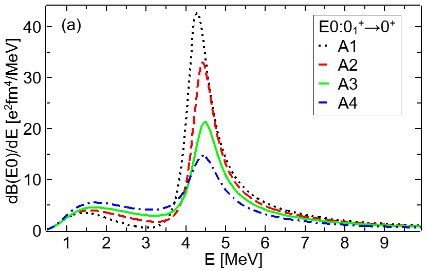
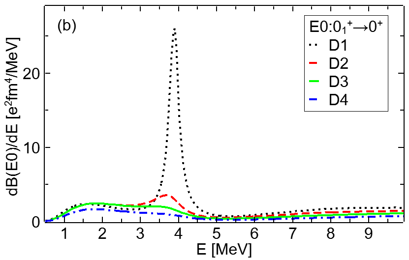
Figure 1: (Color online) The E0-TSDs for the transition from ¹²C${(0_{1}^{+})}$ to $3\alpha(0^{+})$ states. Dotted (black), dashed (red), solid (green), and dot-dashed (blue) curves denote calculations with A1 [D1], A2 [D2], A3 [D3], and A4 [D4] models, respectively in (a) [(b)]. Note that peaks of the Hoyle state are not displayed in these figures, but their peak values are shown in Table 5.

There have been some debates on the nature of the $0_{3}^{+}$ peak. The energy spectrum for a reaction to produce a sharp resonance state just above the threshold energy, e.g., ${}^{9}\mathrm{Be}(p,d){}^{8}\mathrm{Be}$ reaction, sometimes reveals an additional small and broad peak at an energy above the resonance peak [42, 43], which is called as Ghost Anomaly. In a R-matrix theory of the resonance formula [44], this peak is considered to be caused as a result of rather rapid energy-dependence of a resonance decay width parameter arising from the Coulomb penetration factor.

In recent analysis of the inclusive excitation-energy spectra in ${}^{12}\mathrm{C}(\alpha,\alpha^{\prime}){}^{12}\mathrm{C}$ and ${}^{14}\mathrm{C}(p,t){}^{12}\mathrm{C}$ reactions in terms of a multi-level, multi-channel R-matrix theory [12, 13], the $0_{3}^{+}$ peak (denoted as $0_{\Delta}^{+}$ in the references) turns to be an additional resonance state because the Ghost peak associated with the Hoyle state does not have enough strength to explain the experimental data.

To examine the $0_{3}^{+}$ peak in the present $3\alpha$ model, the Hoyle state peak for the D3 model is fitted by R-matrix parameterization as in Ref. [12]. In Fig. 2, thus calculated E0-TSDs in R-matrix with taking several values of the channel radius parameter $a$, are compared with the D3 result. As shown in Fig. 2, the R-matrix calculations reveal the Ghost peak, but their strengths are quite small compared to the D3 calculation, which is not enough to reproduce the experimental data as in Ref. [12]. As the channel radius $a$ increases, the energy of the Ghost peak is shifted to lower energy and the strength becomes weak. Note that the channel radius $a=11$ fm was used in Ref. [12]. Thus, a large part of the $0_{3}^{+}$ peak may be caused by a resonance pole with a minor contribution of the Ghost peak.

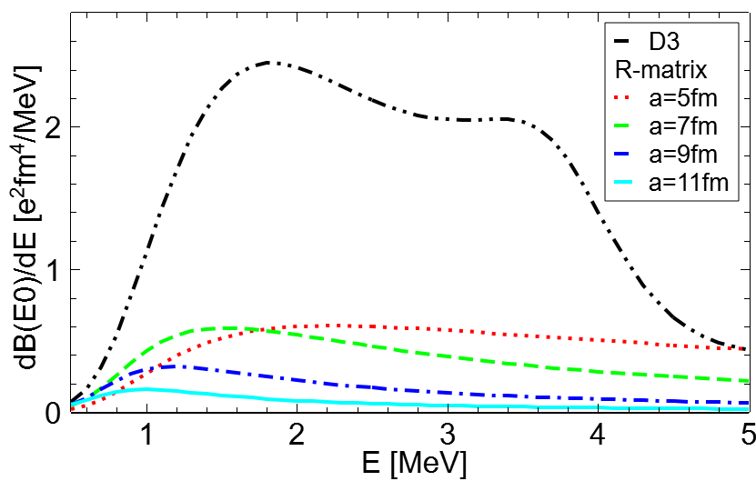
Figure 2: (Color online) The E0-TSDs for the transition from ¹²C${(0_{1}^{+})}$ to $3\alpha(0^{+})$ states. Dot-dot-dashed (black) curve denotes the calculations of the D3 model. Dotted (red), dashed (green), dot-dashed (blue), and solid (cyan) curves denote calculations by the R-matrix formula with the channel radius parameters $a=$ 5 fm, 7 fm, 9 fm, and 11 fm, respectively.

III.3 $3\alpha(2^{+})$ states

III.3.1 ${}^{12}\rm{C}(2_{1}^{+})$ state

As mentioned previously, the strength parameter of the $3\alpha$P for $3\alpha(2^{+})$ state is determined to reproduce the energy of the first excited state ${}^{12}\rm{C}(2_{1}^{+})$. In Table 6, calculated energies, the reduced E2 transition strength between the ground state and the first excited state, $B(\mathrm{E2}:2_{1}^{+}\to 0_{1}^{+})=B(\mathrm{E2}:0_{1}^{+}\to 2_{1}^{+})/5$, and the quadrupole moment $Q_{\mathrm{S}}(2_{1}^{+})=0.75793\langle 2_{1}^{+}||\mathrm{E}2||2_{1}^{+}\rangle$ [45], are shown. In the recent measurement in an electron scattering [46], the value of $7.63(19)~e^{2}\mathrm{fm}^{4}$ is obtained for $B(\mathrm{E2}:2_{1}^{+}\to 0_{1}^{+})$, which is consistent with other electron scattering results reported in the compilation [47]: $[7.94(66),7.72(74),8.12(82),9.4(2.0)]~e^{2}\mathrm{fm}^{4}$, and also with those obtained from $(\alpha,\alpha^{\prime})$ reactions: $7.68(1.00)~e^{2}\mathrm{fm}^{4}$ [48] and $7.4(2)~e^{2}\mathrm{fm}^{4}$ [8].

The calculated values of $B(\mathrm{E2}:2_{1}^{+}\to 0_{1}^{+})$ correlate well with the $3\alpha$P range parameter $a_{3}$ in Eq. (19), and the experimental value of [46] gives the range parameter $a_{3}=3.7$ fm for the AB(A’) + $3\alpha$P calculations and $a_{3}=3.1$ fm for the AB(D) + $3\alpha$P calculations, which supports the A1, A2, D2, and D3 models.

Also in Ref. [46], using a correlation between calculated values of $B(\mathrm{E2}:2_{1}^{+}\to 0_{1}^{+})$ and those of the quadrupole moment $Q_{\mathrm{S}}(2_{1}^{+})$ obtained with ab initio calculations based on the no-core shell model [49], $Q_{\mathrm{S}}(2_{1}^{+})=5.97(30)~e\mathrm{fm}^{2}$ was extracted.

For the present $3\alpha$ model calculations, the correlation between $B(\mathrm{E2}:2_{1}^{+}\to 0_{1}^{+})$ and $Q_{\mathrm{S}}(2_{1}^{+})$ is also observed for each of the $2\alpha$P. The use of the AB(A’) + $3\alpha$P models results $Q_{\mathrm{S}}(2_{1}^{+})=6.41(46)~e\mathrm{fm}^{2}$ while that of AB(D) + $3\alpha$P models does $Q_{\mathrm{S}}(2_{1}^{+})=6.09(18)~e\mathrm{fm}^{2}$. These values agree with the one obtained in Ref. [46], which suggests the correlation between $B(\mathrm{E2}:2_{1}^{+}\to 0_{1}^{+})$ and $Q_{\mathrm{S}}(2_{1}^{+})$ is less nuclear model dependent.

The experimental value of $Q_{\mathrm{S}}(2_{1}^{+})$ has been measured by the Coulomb-excitation of ¹²C by a heavy ion target. The theoretical values above obtained for $Q_{\mathrm{S}}(2_{1}^{+})$ are consistent with experimental value of Ref. [50], $Q_{\mathrm{S}}(2_{1}^{+})=+6(3)~e\mathrm{fm}^{2}$, and that of Ref. [51], $Q_{\mathrm{S}}(2_{1}^{+})=+7.1(2.5)~e\mathrm{fm}^{2}$, but not consistent with the recent value, $Q_{\mathrm{S}}(2_{1}^{+})=+9.5(1.8)~e\mathrm{fm}^{2}$, obtained in Ref. [45].

Table 6: Calculated values of the binding energy, E2 transition strength, and quadrupole moment of ${}^{12}\rm{C}(2_{1}^{+})$.

	Binding energy	$B(\mathrm{E2}:2_{1}^{+}\to 0_{1}^{+})$	$Q_{\mathrm{S}}(2_{1}^{+})$
Model	MeV	$e^{2}\mathrm{fm}^{4}$	$e\mathrm{fm}^{2}$
Exp.	2.8348	7.63(19)	6(3)
AB(A’) + $3\alpha$P
A1	2.848	8.68	6.65
A2	2.841	6.86	6.29
A3	2.836	5.74	5.95
A4	2.840	4.66	5.43
AB(D) + $3\alpha$P
D1	2.851	9.43	6.46
D2	2.830	8.20	6.25
D3	2.832	7.32	6.05
D4	2.837	6.15	5.78

III.3.2 $3\alpha(2^{+})$ continuum states

Calculated E2-TSDs for the transition from the ¹²C${(0_{1}^{+})}$ state to $3\alpha(2^{+})$ continuum states are shown in Fig. 3 (a) for the AB(A’) + $3\alpha$P models and in Fig. 3 (b) for the AB(D) + $3\alpha$P models as functions of the energy $E$. A common feature of all the calculated E2-TSDs is the existence of peaks at $E\approx 2$ MeV and at $E\approx 7$ MeV, although the latter peaks for the AB(A’) + $3\alpha$P models are rather indistinct. In addition to these peaks, a tiny structure can be seen around $E=4.5$ MeV in the E2-TSDs as demonstrated in the inset of Fig. 3 (b). The existence of $3\alpha(2^{+})$ state at this energy region has been reported previously in analises of ${}^{11}\mathrm{B}({}^{3}\mathrm{He},d){}^{12}\mathrm{C}$ reaction [52], ¹²B and ¹²N $\beta$-decay data [53], and $(\alpha,\alpha^{\prime})$ reaction [48]. This $2^{+}$ state was once adapted as $(E_{r},\Gamma_{3\alpha})=$(3.89 MeV, 0.43 MeV) in the compilations [4, 5], but disappears in the most recent compilation [6] after the experimental reports to show negative evidence for it [9, 54]. Theoretically, the existence of $3\alpha(2^{+})$ state around $E=4$ MeV has been shown in semi-microscopic $3\alpha$ cluster model calculations [15, 16] and a $3\alpha$ model calculation with the hyperspherical adiabatic formalism [55].

Here, I examined a monopole transition to $3\alpha(2^{+})$ continuum states from the ¹²C${(2_{1}^{+})}$ state instead of the ¹²C${(0_{1}^{+})}$ state. In Fig. 3 (c), the E0-TSDs for this transition for the A2, A3, D2, and D3 models are shown. These functions show clear peaks around $E\approx 4.5$ MeV, which indicates the existence of a resonance state. Meanwhile, as demonstrated in Figs. 3 (a) and (b), the E2 transition strength of this state from the ¹²C${(0_{1}^{+})}$ state is small, and this might be the reason why the existence of this state has not been clearly established.

Hereafter, the peaks at $E\approx 2$ MeV, $E\approx 4.5$ MeV, and $E\approx 7$ MeV will be designated as $2_{2}^{+}$, $2_{3}^{+}$, and $2_{4}^{+}$ states, respectively. The resonance parameters, $E_{r}$ and $\Gamma_{3\alpha}$, which are obtained by analyzing adequate peaks of the TSDs in Fig. 3 with Eq. (17) are shown in Table 7.

As mentioned in the introduction, the existence of the $2_{2}^{+}$ state in ¹²C has been reported in some experimental works and the experimental values of $\left(E_{r},\Gamma_{3\alpha}\right)$ in MeV are $\left[2.3(1),0.6(1)\right]$ in $(p,p^{\prime})$ data [7, 9], $\left[2.57(6),1.01(15)\right]$ in $(\alpha,\alpha^{\prime})$ data [8], $\left[2.48(15),0.750(150)\right]$ in combined analysis [10] of the data in Refs. [7, 8], $\left[2.76(11),0.800(130)\right]$ in $(\gamma,\alpha)$ [11], and $\left[2.751(50),1.60(13)\right]$ in reanalysis of the data [11], which is cited in Ref. [3]. The calculated values of the resonance energy and the $3\alpha$-decay width from by the present $3\alpha$ calculations in Table 7 are rather model independent and are consistent with these experimental values.

The E2 strength of the $2_{2}^{+}$ state $B(\mathrm{E2}:0_{1}^{+}\to 2_{2}^{+})$ in Table 7 is evaluated by integrating the E2-TSD for $E<3.5$ MeV, which indicates that this strength largely depends on the range parameters of $2\alpha$P and $3\alpha$P. It is noted that theoretical values by microscopic calculations also show a large model dependence: $2~e^{2}\mathrm{fm}^{4}$ [20, 56] and $10(5)~e^{2}\mathrm{fm}^{4}$ [22].

Experimental results for $B(\mathrm{E2}:0_{1}^{+}\to 2_{2}^{+})$ are rather scattered: $1.83(9)~e^{2}\mathrm{fm}^{4}$, $1.6(2)~e^{2}\mathrm{fm}^{4}$ in $(\alpha,\alpha^{\prime})$ reaction [8], $2.5(5)~e^{2}\mathrm{fm}^{4}$ in $(\alpha,\alpha^{\prime})$ reaction [48] as cited in Ref. [56], 3.7(65) $e^{2}\mathrm{fm}^{4}$ from $(\gamma,\alpha)$ reaction Ref. [11], and $14(+1.5,-2.0)~e^{2}\mathrm{fm}^{4}$ in reanalysis of the data [11], which is cited in Ref. [3]. Considering a large model dependence of $B(\mathrm{E2}:0_{1}^{+}\to 2_{2}^{+})$, more precise experimental infomation of this strength is desirable.

Although the peaks corresponding to $2_{4}^{+}$ state in the E2-TSD for the AB(D) + $3\alpha$P models are clear, those for the AB(A’) + $3\alpha$P models are not so clear due to broader widths. This peak may correspond to the $2^{+}$ resonance state: $(E_{r},\Gamma_{3\alpha})=$ [8.17(40) MeV, 1.77(20) MeV] reported in Ref. [6] with uncertainty as shown in Table 1.

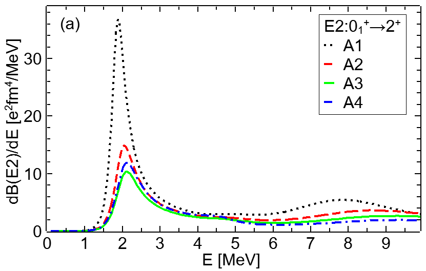
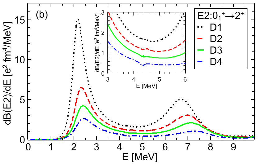
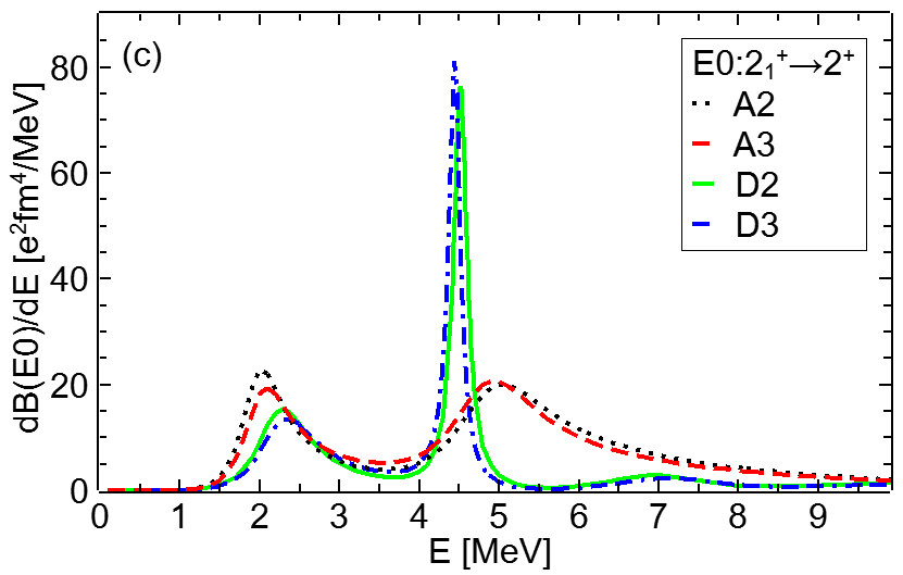
Figure 3: (Color online) (a) and (b): The E2-TSDs for the transition from ¹²C${(0_{1}^{+})}$ to $3\alpha(2^{+})$ states. (c) The E0-TSDs for the transition from ¹²C${(2_{1}^{+})}$ to $3\alpha(2^{+})$ states. In (a) [(b)], dotted (black), dashed (red), solid (green), and dot-dashed (blue) curves denote the calculations of the A1 [D1], A2 [D2], A3 [D3], and A4 [D4] models, respectively. Inset in (b) is the magnification around $E=4.5$ MeV. In (c), dotted (black), dashed (red), solid (green), and dot-dashed (blue) curves denote calculations with the A2, A3, D2, and D3 models, respectively.

Table 7: Calculated values of the resonance energy and the $3\alpha$-decay width for $2_{2}^{+}$, $2_{3}^{+}$, and $2_{4}^{+}$ states, and the E2 transition strength for $2_{2}^{+}$ state.

	$E_{r}(2_{2}^{+})$	$\Gamma_{3\alpha}(2_{2}^{+})$	$B(\mathrm{E2}:0_{1}^{+}\to 2_{2}^{+})$	$E(2_{3}^{+})$	$\Gamma_{3\alpha}(2_{3}^{+})$	$E_{r}(2_{4}^{+})$	$\Gamma_{3\alpha}(2_{4}^{+})$
Model	MeV	MeV	$e^{2}\mathrm{fm}^{4}$	MeV	MeV	MeV	MeV
AB(A’) + $3\alpha$P
A1	2.0	0.9	27.1	5.1	1.5	7.9	4.2
A2	2.2	1.0	15.0	5.1	1.8	8.7	5.2
A3	2.2	1.0	11.5	5.0	1.8	9.2	5.8
A4	2.2	1.0	13.2	4.8	1.5	9.4	6.5
AB(D) + $3\alpha$P
D1	2.3	0.9	13.5	4.6	0.2	6.6	1.8
D2	2.5	0.9	7.1	4.5	0.2	6.9	1.8
D3	2.5	0.8	4.9	4.5	0.2	7.1	1.8
D4	2.5	0.9	3.1	4.4	0.2	7.2	1.9

III.4 $3\alpha(1^{-})$ and $3\alpha(3^{-})$ states

Since there is no bound state for $3\alpha(1^{-})$ and $3\alpha(3^{-})$ states, the $3\alpha$P strength parameters for these states in Table 3 are determined to reproduce the energy of the lowest resonance state shown in Table 1 by the energy of the first maximum in calculated TSD. Calculated E1- and E3-TSDs for some selected models are shown in Fig. 4.

The $3\alpha$-decay width and the E$\lambda$ strength calculated by fitting these TSDs to the resonance formula Eq. (17) are shown in Tables 8 and 9 for $3\alpha(1^{-})$ and $3\alpha(3^{-})$ states, respectively.

III.4.1 ${}^{12}\rm{C}(1_{1}^{-})$ state

Calculated values of $\Gamma_{3\alpha}(1_{1}^{-})$ for the AB(D) + $3\alpha$P models are consistent with the experimental value, but those for the AB(A’) + $3\alpha$P models are about 40% larger than the experimental value. The correlation between $\Gamma_{3\alpha}(1_{1}^{-})$ and the $3\alpha$P range parameter with the experimental value of $\Gamma_{3\alpha}(1_{1}^{-})$ gives $a_{3}=3.1$ fm for the AB(D) + $3\alpha$P models.

Although the dependence of the E1 strength on the $3\alpha$P range parameter is remarkable, there is no experimental information for these values in Ref. [6].

For the AB(D) + $3\alpha$P models, there appears another $1^{-}$ resonance peak at $E\sim 7$ MeV to 8 MeV, but there has not been reported corresponding resonance state to this in the compilations so far [4, 5, 6].

III.4.2 ${}^{12}\rm{C}(3_{1}^{-})$ state

Calculated values of $\Gamma_{3\alpha}(3_{1}^{-})$ have a weak dependence on the choice of the $3\alpha$P, but are determined essentially by $2\alpha$P: about 55 keV for the AB(A’) + $3\alpha$P calculations and 32 keV for the AB(D) + $3\alpha$P calculations. The adapted value in the compilation [6], $\Gamma_{3\alpha}(3_{1}^{-})=46(3)$ keV, was recently criticized in Ref. [57] to be updated by a smaller value, 38(2) keV. One of the grounds of this argument is related to the definition of the total decay width in the R-matrix parameterization. In the analysis of the R-matrix, an energy-dependent total decay width, which is referred to as a formal decay width (see Eq. (3) of Ref. [57]), is highly model (in this case the channel radius parameter $a$) dependent and should not used for an intrinsic decay width, which is approximated by the observed total width, Eq. (8) in Ref. [57]. Actually, when the E3-TSF of the D3 model is fitted by the R-matrix parametrization with $a=4.0$ fm, the formal decay width at the resonance peak energy becomes 48 keV, and the observed total width becomes 32 keV. Also, the formal (observed) decay width with $a=5$ fm becomes 36 keV (32 keV). Thus the observed total width is model-independent and well agrees with the total width calculated from the line shape of the E3-TSF by Eq. (17). Thus the values of $\Gamma_{3\alpha}(3_{1}^{-})$ in Table 9 should be compared to a smaller value, e.g., $38(2)$ keV, not $46(3)$ keV.

Calculated values of the $B(\mathrm{E}3:0_{1}^{+}\to 3_{1}^{-})$ strength are largely model dependent. However, experimental values are also widely distributed as follows: In the compilation literature [58], the value $6.1(0.9)\times 10^{2}~e^{2}\mathrm{fm}^{6}$ is adapted taking values obtained from inelastic $(e,e^{\prime})$ scattering: $7.5(1.0)\times 10^{2}~e^{2}\mathrm{fm}^{6}$ [59] and $4.75(1.20)\times 10^{2}~e^{2}\mathrm{fm}^{6}$ [60, 61]. On the other hand, values of $2.4(4)\times 10^{2}~e^{2}\mathrm{fm}^{6}$ [48] and $2.51(10)\times 10^{2}~e^{2}\mathrm{fm}^{6}$ [8] were obtained from inelastic $(\alpha,\alpha^{\prime})$ scattering.

For the AB(D) + $3\alpha$P models, there appears another $3^{-}$ resonance peak for $E>9$ MeV. This peak could correspond to the $3^{-}$ resonance state: $(E_{r},\Gamma_{3\alpha})=$ [11.3(1) MeV, 0.3 MeV] reported in Refs. [4, 5, 6] as shown in Table 1, although its isospin is not specified.

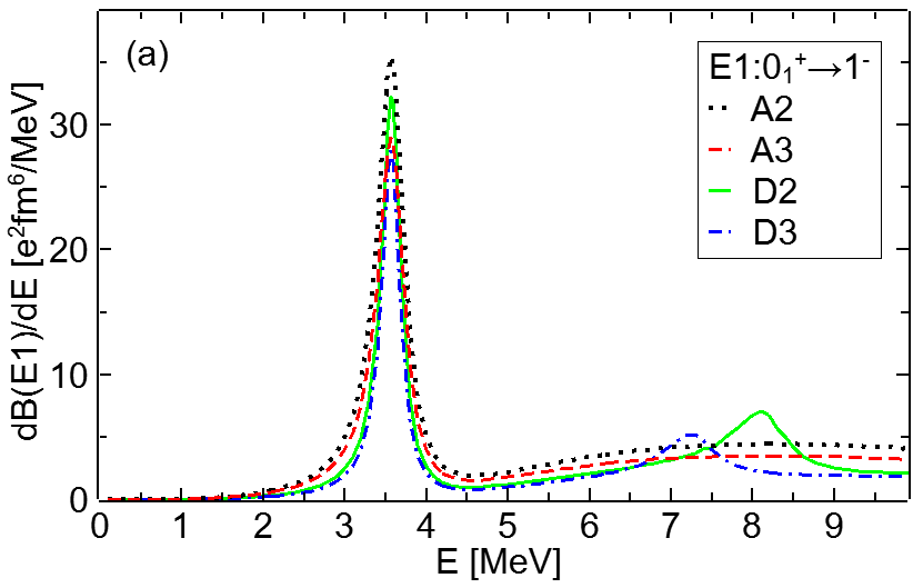
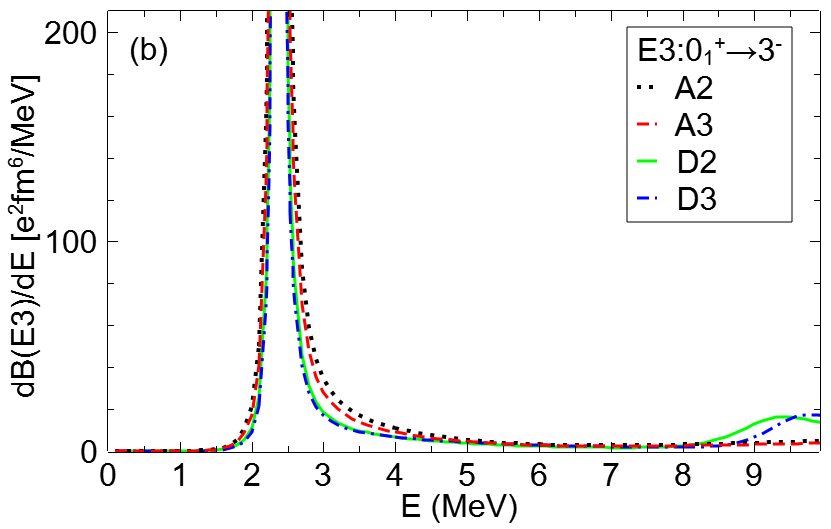
Figure 4: (Color online) (a) The E1-TSDs for the transition from ¹²C${(0_{1}^{+})}$ to $3\alpha(1^{-})$ state, and (b) the E3-TSDs for the transition from ¹²C${(0_{1}^{+})}$ to $3\alpha(3^{-})$ states. Dotted (black), dashed (red), solid (green), and dot-dashed (blue) curves denote calculations with the A2, A3, D2, and D3 models, respectively.

Table 8: Calculated values of decay widths and E1 transition strengths for the $3\alpha(1_{1}^{-})$ state.

	$\Gamma_{3\alpha}(1_{1}^{-})$	$B(\mathrm{E1}:0_{1}^{+}\to 1_{1}^{-})$
Model	keV	$e^{2}\mathrm{fm}^{6}$
Exp.	273(5)
AB(A’) + $3\alpha$P
A1	412	30
A2	392	21
A3	383	16
A4	382	15
AB(D) + $3\alpha$P
D1	297	21
D2	282	14
D3	268	12
D4	251	9.0

Table 9: Calculated values of decay widths and E3 transition strengths for the $3\alpha(3_{1}^{-})$ state.

	$\Gamma_{3\alpha}(3_{1}^{-})$	$B(\mathrm{E3}:0_{1}^{+}\to 3_{1}^{-})$
Model	keV	$e^{2}\mathrm{fm}^{6}$
Exp.	46(3)
	38(2)
AB(A’) + $3\alpha$P
A1	58	895
A2	56	638
A3	56	525
A4	55	491
AB(D) + $3\alpha$P
D1	30	753
D2	31	595
D3	32	503
D4	32	388

IV Excitation-energy spectrum

In general, experimental information of the electric multipole transition strength distributions studied in the previous section is included in cross sections of reactions leading to $3\alpha$ continuum states in the final state. In this section, I will study the excitation-energy spectra in the $\alpha$-induced inelastic scattering ${}^{12}\mathrm{C}(\alpha,\alpha^{\prime})3\alpha$ at $E_{\alpha,\mathrm{Lab}}=386$ MeV [8]. Calculations will be performed in PWIA, where the incident $\alpha$-particle collides with an $\alpha$-particle in the target, and is scattered to a certain solid angle $\Omega$ leaving $3\alpha$ with the excitation energy $E_{x}$ in the laboratory (Lab.) frame. In this framework, the cross section is written in a factorized form,

$$\frac{d^{2}\sigma}{d\Omega dE_{x}}=N_{K}\sigma_{\alpha\alpha}R(E,Q),$$ (23)

where $Q$ is the momentum transfer. A kinematical factor $N_{K}$ and some other related kinematical variables are given in Appendix B. The variable $\sigma_{\alpha\alpha}$ is the cross section for the elementary process: $\alpha$-$\alpha$ scattering at $E_{\alpha,\mathrm{Lab}}=386$ MeV. Since there is no available experimental data for the $\alpha$-$\alpha$ elastic scattering at this energy region, in the present calculations, $\sigma_{\alpha\alpha}$ is taken to be the $\alpha$-$\alpha$ Coulomb (Rutherford) differential cross section as function of the momentum transfer $Q$,

$$\sigma_{\alpha\alpha}=\sigma_{C}(Q)=\left(\frac{\mu_{\alpha\alpha}Z_{1}Z_{2}e^{2}}{\hbar^{2}}\right)^{2}\frac{4}{Q^{4}},$$ (24)

where $\mu_{\alpha\alpha}$ is the reduced mass of $2\alpha$ system and $Z_{1}=Z_{2}=2$. The factor $R(E,Q)$ is the response function corresponding to the transition from the $3\alpha$ bound state $|\Psi_{b}(J_{i}M_{i})\rangle$ with angular momentum $J_{i}$ and its third component $M_{i}$ to $3\alpha$-continuum states with energy $E$,

$$R(E,Q)=\frac{1}{2J_{i}+1}\sum_{J_{i}M_{i}}\int d\bm{q}^{\prime}d\bm{p}^{\prime}\delta\left(E-E^{\prime}\right)\left|\langle\Psi^{(-)}_{\bm{q}^{\prime},\bm{p}^{\prime}}(E^{\prime})|\sum_{i=1,3}e^{i\bm{Q}\cdot\bm{r}_{i}}|\Psi_{b}(J_{i}M_{i})\rangle\right|^{2},$$ (25)

where $\bm{Q}$ is the momentum transfer vector. By taking the lowest order term in each of the multipole ($\lambda$) expansion of $e^{i\bm{Q}\cdot\bm{r}_{i}}$ up to $\lambda=3$, one has

$$R(E,Q)=\sum_{\lambda=0,3}a_{\lambda}(Q)\frac{1}{4e^{2}}\frac{dB(\mathrm{E}\lambda:J_{i}\to J_{f})}{dE},$$ (26)

where

$$a_{\lambda}(Q)={(4\pi)^{2}}\times\left\{\begin{array}[]{cc}(Q^{2}/6)^{2}/(4\pi)&(\mathrm{for}~\lambda=0)\\ (Q^{3}/30)^{2}&(\mathrm{for}~\lambda=1)\\ (Q^{2}/15)^{2}&(\mathrm{for}~\lambda=2)\\ (Q^{3}/105)^{3}&(\mathrm{for}~\lambda=3).\end{array}\right.$$ (27)

In this work, theoretical the cross section for the ${}^{12}\mathrm{C}(\alpha,\alpha^{\prime})3\alpha$ reaction is expressed in the following form:

$$\frac{d^{2}\sigma}{d\Omega dE_{x}}=N_{K}\frac{\sigma_{\alpha\alpha}}{4e^{2}}\sum_{\lambda=0,3}x_{\lambda}a_{\lambda}(Q)\frac{dB(\mathrm{E}\lambda:J_{i}\to J_{f})}{dE},$$ (28)

where the extra parameters $x_{\lambda}~(\lambda=0,...,3)$ are introduced to take into account of various effects that are not incorporated in PWIA.

To compare calculations with the data, possible experimental resolutions are taken into account by convoluting Eq. (28) with a Gaussian function of a full width at half maximum (FWHM). Thus fitting parameters in this work are weight factors of multipole components, $x_{\lambda}~(\lambda=0,1,2,3)$ in Eq. (28) and the convolution FWHM. The FWHM was searched for values between 100 keV and 250 keV with a step 10 keV because the value of 200 keV was quoted as the resolution in Ref. [8]. These parameters are determined to reproduce the experimental data in Ref. [8] for $8~\mathrm{MeV}<E_{x}<12~\mathrm{MeV}$.

For the ${}^{12}\mathrm{C}(\alpha,\alpha^{\prime})$ reaction at $E_{\alpha,\mathrm{Lab}}=386$ MeV with $\theta=0^{\circ}$, the momentum transfer $Q$ takes 0.09 $\mathrm{fm}^{-1}$ at $E_{x}=8$ MeV and 0.14 $\mathrm{fm}^{-1}$ at $E_{x}=12$ MeV, and $N_{K}\approx 17.6$ through out the excitation energy range.

It turns out that models other than the D2, D3, and D4 are not adequate to fit the experimental data with good quality mainly because of a large strength of $0_{4}^{+}$ compared to $0_{3}^{+}$ as explained below. The convolution FWHM=140 keV is best to obtain a good fit. Fitted parameters $x_{\lambda}~(\lambda=0,\dots,3)$ are shown in Table 10, and results of the spectrum are displayed in Fig. 5. The spectrum consists of a sharp peak around $E_{x}=9.6$ MeV, which corresponds to $3_{1}^{-}$ state, on the top of a broad bump contributed from $0^{+}$, $1^{-}$, and $2^{+}$ states.

Although the $x_{\lambda}$-parameter search was performed automatically, the results can be interpreted as follows. The lower part of the broad bump, $E_{x}<9$ MeV, mainly consists of the $0_{3}^{+}$ state, and the parameter $x_{0}$ is determined to fit the spectrum in this region. Then, the spectrum around the sharp peak consists of $2^{+}$ and $3^{-}$ states as well as the fixed $0^{+}$ state, from which the parameters $x_{2}$ and $x_{3}$ are determined. Finally, the rest parameter $x_{1}$ is determined to reproduce the upper part of the broad peak, $E_{x}>10.5$ MeV.

For D2, since the contribution of the $0_{4}^{+}$ peak is large and even exceeds the experimental data for $E_{x}>11$ MeV, there is no room for the $1_{1}^{-}$ state. On the other hand, for D3 and D4, because of not too large contributions of the $0_{4}^{+}$ state, a room for the $1_{1}^{-}$ state together with the high energy tail of the $2_{2}^{+}$ peak, is left. But it is remarked that the discrepancies between calculations and the data around $E=10.5$ MeV are left even for these models.

For all of these models, the peak at $E_{x}\approx 9.7$ MeV consists of the $3_{1}^{-}$ state together with rather broad $2_{2}^{+}$ peak and $0^{+}$ contributions.

The other models than the D2, D3, and D4, if the spectrum around $E_{x}=9$ MeV is fitted by the $0_{3}^{+}$ peak, contributions from the $0_{4}^{+}$ peak are too large to get a good fit.

Table 10: Parameters to fit the experimental energy spectra for the ${}^{12}\mathrm{C}(\alpha,\alpha^{\prime})$ reaction at scattering angle $\theta_{\mathrm{lab}}=0^{\circ}$ [8] for the D2, D3, and D4 models.

Model	$x_{0}$	$x_{1}$	$x_{2}$	$x_{3}$
D2	0.957	0.509	0.102	2.66
D3	1.15	1.34	0.128	2.78
D4	1.59	5.12	0.295	3.23

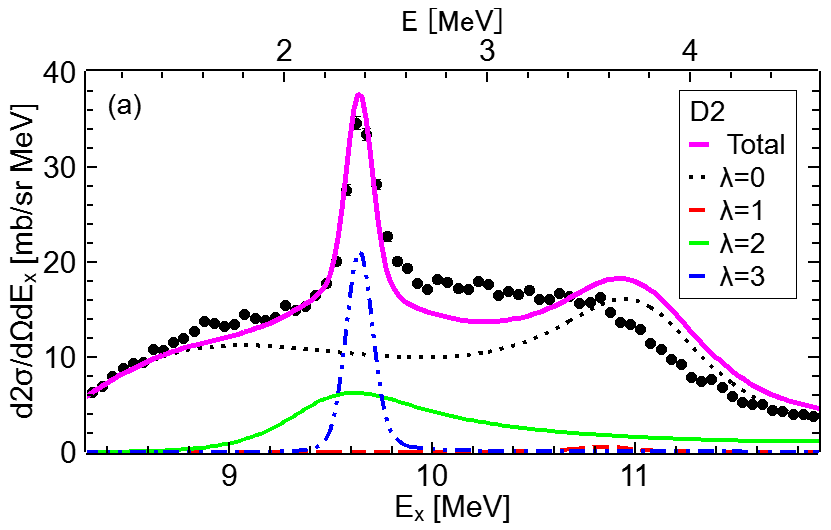
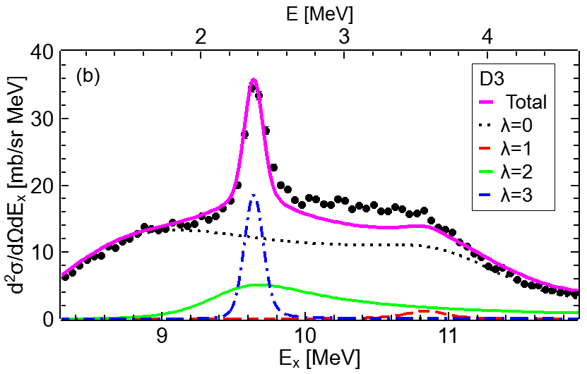
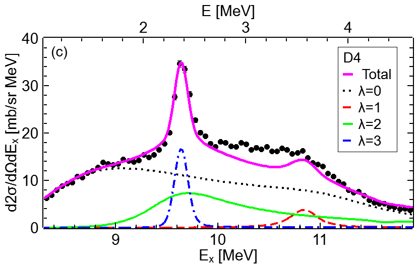
Figure 5: (Color online) Energy spectra for the ${}^{12}\mathrm{C}(\alpha,\alpha^{\prime})$ reaction at scattering angle $\theta_{\mathrm{lab}}=0^{\circ}$ for (a) D2, (b) D3, and (c) D4 models. Bold solid (magenta), dotted (black), dashed (red), solid (green), and dot-dashed (blue) curves denote total, $\lambda=0$, 1, 2, and 3 contributions, respectively. Experimental data are taken from Ref. [8].

For the measurement of ${}^{12}\mathrm{C}(\alpha,\alpha^{\prime})$ reaction at $E_{\alpha,\mathrm{Lab}}=386$ MeV with $\theta=3.7^{\circ}$, the momentum transfer $Q$ takes about 0.6 $\mathrm{fm}^{-1}$ and $N_{K}\approx 17.6$ through out the energy range considered in this work.

The cross section for the measurement of ${}^{12}\mathrm{C}(\alpha,\alpha^{\prime})$ reaction at $E_{\alpha,\mathrm{Lab}}=386$ MeV with $\theta=3.7^{\circ}$ is shown in Fig. 6 for the D3 model. In this case, the contribution from $\lambda=3$ TSD dominates the spectrum and that from $\lambda=2$ TSD adds some component and other $\lambda=0$ and $\lambda=1$ contributions are small. In the D3 model, fitted parameters are: $x_{0}=0.0692$, $x_{1}=0.0579$, $x_{2}=0.201$, and $x_{3}=0.362$ with FWHM=140 keV.

The existence of a peak corresponding $2_{3}^{+}$ state, which is predicted in the $3\alpha$ model, is not clear, because the cross sections for this state is too small and smeared out by the convolution.

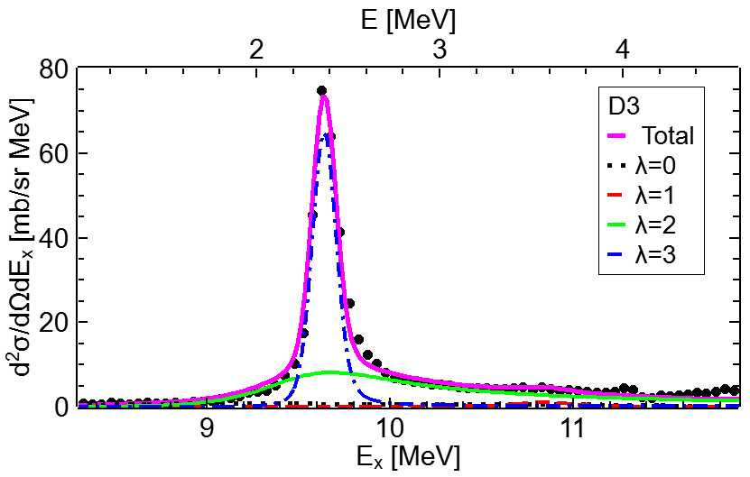
Figure 6: (Color online) Energy spectra for the ${}^{12}\mathrm{C}(\alpha,\alpha^{\prime})$ reaction at scattering angle $\theta_{\mathrm{lab}}=3.7^{\circ}$ for the D3 model. Magenta, black, red, green, and blue curves denote total, $\lambda=0$, 1, 2, and 3 contributions, respectively. Experimental data are taken from Ref. [8].

Finally, I will analyze the cross section data around the Hoyle state. Experimental data of the energy spectrum at $\theta_{\mathrm{Lab}}=0^{\circ}$ for $7.4~\mathrm{MeV}<E_{x}<7.9~\mathrm{MeV}$ are fitted by a Gaussian distribution

$$\frac{d^{2}\sigma}{d\Omega dE_{x}}=\left(\frac{N_{K}\sigma_{\alpha\alpha}a_{0}}{4}\right)\frac{x_{0}B_{0}}{e^{2}}\frac{1}{\sigma\sqrt{2\pi}}\exp\left(-\frac{(E_{x}-E_{r})^{2}}{2\sigma^{2}}\right),$$ (29)

where $E_{r}=7.65$ MeV and $N_{k}\sigma_{\alpha\alpha}a_{0}/4=4.750$ $\mathrm{fm}^{-4}$ mb/sr. The experimental data is well fitted with $x_{0}B_{0}=16.4~e^{2}\mathrm{fm}^{4}$ and $\sigma=0.0724$ MeV (FWHM =170 keV) as shown in Fig. 7.

This fitted value of $x_{0}B_{0}$ is about 60% of those calculated from the fitted values for the spectra of higher excitation-energy in Table 10 together with the values of $B(\mathrm{E0}:0_{1}^{+}\to 0_{2}^{+})$ in Table 5: $x_{0}B_{0}=(27.7,28.5,28.0)~e^{2}\mathrm{fm}^{4}$ for the D2, D3, and D4 models, respectively. In other words, the use of the parameters determined for resonance states at higher energies results the Hoyle state peak being overestimated. This is known as the missing monopole strength of the Hoyle state [62], which may occur due to the use of PWIA in the present calculations. It is suggested that adequate treatments of distorting waves in initial and final states are necessary to resolve this problem [63].

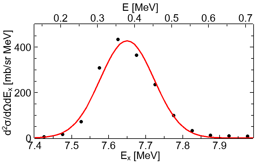
Figure 7: (Color online) Energy spectra for the ${}^{12}\mathrm{C}(\alpha,\alpha^{\prime})$ reaction at scattering angle $\theta_{\mathrm{lab}}=0^{\circ}$. Red curve is the result of Gaussian fit with Eq. (29). Experimental data are taken from Ref. [8].

V Summary

In this paper, low-energy continuum states as well as bound states in the ¹²C nucleus are studied by the $3\alpha$ models, where several sets of $2\alpha$- and $3\alpha$ potential models are introduced. The electric multipole strength distributions for the transition of ${}^{12}\mathrm{C}(0_{1}^{+})$ state to $3\alpha$ continuum states with $J^{\pi}=0^{+},1^{-},2^{+}$, and $3^{-}$ are calculated, from which model dependence is studied for various observables such as the $3\alpha$-decay width and the electric multipole strength of $3\alpha$ resonance states. Using calculated strength distributions, the excitation energy spectra of the forward ${}^{12}\mathrm{C}(\alpha,\alpha^{\prime})3\alpha$ reaction at $E_{\alpha,\mathrm{Lab}}=386$ MeV are calculated, and compared with the available experimental data.

Two different versions of the $2\alpha$P, AB(A’) and AB(D), are used in the present calculations, which are two-range Gaussian-type along with the $\alpha$-$\alpha$ Coulomb potential. The $3\alpha$ potential models are constructed assuming some values of the range parameters with Gaussian form, and thus the strength parameters are determined to reproduce the energies: $E_{r}(0_{2}^{+})$, $E_{r}(1_{1}^{-})$, $E(2_{1}^{+})$, and $E_{r}(3_{1}^{-})$.

Of several models examined, the combination of AB(D) and $3\alpha$P with the range parameters $a_{3}=3.0$ fm (D3) can be recommended although there are some observables to be improved. Main reason of this choice comes from the ratio of the $0_{3}^{+}$ strength to $0_{4}^{+}$ strength, which is important to fit the line shape of ${}^{12}\mathrm{C}(\alpha,\alpha^{\prime})3\alpha$ energy spectrum. In general, a longer range interaction, either $2\alpha$P or $3\alpha$P, results a larger $0_{4}^{+}$ strength.

There remain some rooms to improve interaction models, e.g., to reproduce the energies $E(0_{1}^{+})$ and $E(0_{2}^{+})$ simultaneously.

Lastly, some states in $2^{+}$, $1^{-}$ and $3^{-}$ are observed in the calculations although they are not experimentally confirmed yet possibly because of a weak coupling to the ¹²C ground state and/or a large decay width. For confirming the reliability of the $3\alpha$ model, the existence of these states are quite interesting.

Appendix A Coulomb modified Faddeev equations

In this section, a brief explanation of how to treat the long range Coulomb force in solving Eq. (7) will be given.

For simplicity, $\alpha$-particles are considered to be interacting with two-body potentials only as

$$\hat{V}=\sum_{i=1,3}V_{i}(x_{i})=\sum_{i=1,3}\left[V^{\mathrm{S}}(x_{i})+\frac{(2e)^{2}}{x_{i}}\right],$$ (30)

where $V^{\mathrm{S}}(x)$ is the short range part of the interaction, and in this section I use sets of Jacobi coordinates $\{\bm{x}_{i},\bm{y}_{i}\}$,

$$\bm{x}_{i}=\bm{r}_{j}-\bm{r}_{k},\quad\quad\bm{y}_{i}=\bm{r}_{i}-\frac{1}{2}\left(\bm{r}_{j}+\bm{r}_{k}\right)$$ (31)

with $(i,j,k)$ being $(1,2,3)$ or its cyclic permutations.

I start with the differential equation form of Eq. (7),

$$\left(E-\hat{H}_{3\alpha}\right)|\Xi\rangle=\hat{O}|\Psi_{b}\rangle.$$ (32)

In the Faddeev theory [29], the three-body wave function is decomposed into three Faddeev components,

$$|\Xi\rangle=|\Phi^{(1)}\rangle+|\Phi^{(2)}\rangle+|\Phi^{(3)}\rangle,$$ (33)

and coupled equations of these components (Faddeev equations) describe the multiple scattering of three particles with rearranging the interacting pair. In the case of short range forces, $|\Phi^{(i)}\rangle$ describes a process in which the pair particles $(j,k)$ are interacting while the particle $i$ is free as the spectator. However, in the case of $3\alpha$ system, this picture is not adequate because the spectator $i$ is not free due to the long range Coulomb forces.

To remedy this problem, Coulomb-modified Faddeev equations are introduced as follows [64, 23]:

$$\left[E-H_{0}-V_{1}(x_{1})-\frac{2(2e)^{2}}{y_{1}}\right]|\Phi^{(1)}\rangle = \hat{O}_{1}|\Psi_{b}\rangle+\left[V_{1}(x_{1})-\frac{(2e)^{2}}{y_{2}}\right]|\Phi^{(2)}\rangle$$ (35)

$$+\left[V_{1}(x_{1})-\frac{(2e)^{2}}{y_{3}}\right]|\Phi^{(3)}\rangle,$$

$$\mathrm{(and~cyclic~permutations)},$$ (36)

where the transition operator is decomposed into three components,

$$\hat{O}=\hat{O}_{1}+\hat{O}_{2}+\hat{O}_{3},$$ (37)

with the condition that $\hat{O}_{i}$ is symmetric with respect to the exchange of $j$ and $k$. It is stressed that the original equation (32) is obtained by summing up all equations in (36).

The auxiliary potential $\frac{2(2e)^{2}}{y_{i}}$ in the left hand side of Eq. (36) plays a role to introduce a Coulomb distortion of the spectator $i$. In the right hand side, the auxiliary potentials, $\frac{(2e)^{2}}{y_{2}}$ and $\frac{(2e)^{2}}{y_{3}}$, play a role to cancel the long range components in the potentials $V_{1}(x_{1})$, namely $\frac{(2e)^{2}}{x_{1}}$, which makes the potential terms $(2e)^{2}\left(\frac{1}{x_{1}}-\frac{1}{y_{2}}\right)$ and $(2e)^{2}\left(\frac{1}{x_{1}}-\frac{1}{y_{3}}\right)$, short range functions with respect to the variable $x_{1}$. While this cancellation holds sufficiently for bound states and continuum states below three-body breakup threshold [31], it does insufficiently for the case of the three-body breakup reaction [32]. To avoid difficulties arising from this, a mandatory cutoff factor $e^{-(x/R_{C})^{4}}$ is introduced. This is an approximation made for this calculations, and $R_{C}=35$ fm is used in the calculations, which was found to be enough to obtain converged results [23].

Appendix B Kinematical relations in ${}^{12}\mathrm{C}(\alpha,\alpha^{\prime})3\alpha$ reaction

In this appendix, some kinematical notations and relations to describe the ${}^{12}\mathrm{C}(\alpha,\alpha^{\prime})3\alpha$ reaction treated relativistically in partial are summarized.

Let $T_{i}$ ($T_{f}$) and $\bm{K}_{i}$ ($\bm{K}_{f}$) be the kinetic energy and momentum (wave number), respectively, of the incident $\alpha$-particle (outgoing $\alpha$-particle) in Lab. frame. Here,

$$K_{i} = \sqrt{\left(m_{\alpha}c^{2}+T_{i}\right)^{2}-m_{\alpha}^{2}c^{4}}/(\hbar c)$$ (38)

$$K_{f} = \sqrt{\left(m_{\alpha}c^{2}+T_{f}\right)^{2}-m_{\alpha}^{2}c^{4}}/(\hbar c).$$ (39)

The total energy $E_{\mathrm{tot}}^{(L)}$, energy transfer $\omega^{(L)}$, and momentum transfer $\bm{Q}^{(L)}$ in Lab. frame are

$$E_{\mathrm{tot}}^{(L)} = m_{\alpha}c^{2}+T_{i}+m_{\mathrm{C}}c^{2},$$ (40)

$$\omega^{(L)} = T_{i}-T_{f},$$ (41)

$$\bm{Q}^{(L)} = \bm{K}_{i}-\bm{K}_{f},$$ (42)

where $m_{\mathrm{C}}$ is the mass of the target ¹²C nucleus.

The total energy $E_{tot}^{(c)}$, energy $E_{i}^{(c)}$ and momentum $k_{i}^{(c)}$ of the incident $\alpha$-particle, energy $E_{\mathrm{C}}^{(c)}$ of the target in the initial $\alpha$-${}^{12}\mathrm{C}$ ($\alpha$-C) c.m. frame are

$$E_{tot}^{(c)} = \sqrt{E_{tot}^{(L)2}-(\hbar cK_{i})^{2}},$$ (43)

$$E_{i}^{(c)} = \frac{E_{tot}^{(c)2}+m_{\alpha}^{2}c^{4}-m_{\mathrm{C}}^{2}c^{4}}{2E_{tot}^{(c)}},$$ (44)

$$k_{i}^{(c)} = \sqrt{E_{i}^{(c)2}-m_{\alpha}^{2}c^{4}},$$ (45)

$$E_{\mathrm{C}}^{(c)} = \frac{E_{tot}^{(c)2}-m_{\alpha}^{2}c^{4}+m_{\mathrm{C}}^{2}c^{4}}{2E_{tot}^{(c)}}.$$ (46)

The energy $E_{f}^{(c)}$ and momentum $k_{f}^{(c)}$ of the outgoing $\alpha$-particle, and energy $E_{3\alpha}^{(c)}$ of the $3\alpha$-system in the final $\alpha$-$3\alpha$ c.m. frame are

$$E_{f}^{(c)} = \frac{E_{tot}^{(c)2}+m_{\alpha}^{2}c^{4}-(E_{3\alpha}^{(L)2}-(\hbar cQ^{(L)})^{2})}{2E_{tot}^{(c)}},$$ (47)

$$k_{f}^{(c)} = \sqrt{E_{f}^{(c)2}-m_{\alpha}^{2}c^{4}}/(\hbar c).$$ (48)

$$E_{3\alpha}^{(c)} = \frac{E_{tot}^{(c)2}-m_{\alpha}^{2}c^{4}+(E_{3\alpha}^{(L)2}-(\hbar cQ^{(L)})^{2})}{2E_{tot}^{(c)}},$$ (49)

where

$$E_{3\alpha}^{(L)}=m_{\mathrm{C}}c^{2}+\omega^{(L)}.$$ (50)

The energy transfer $\omega^{(c)}$ and momentum transfer $\bm{Q}^{(c)}$ in the $\alpha$-C c.m. frame are

$$\omega^{(c)} = E_{i}^{(c)}-E_{f}^{(c)}$$ (51)

$$\bm{Q}^{(c)} = \bm{k}_{i}^{(c)}-\bm{k}_{f}^{(c)},$$ (52)

and $Q$ in Eq. (23) is defined as $Q=|\bm{Q}^{(c)}|$.

The energy of the $3\alpha$-system $E$ in the $3\alpha$ c.m. frame is

$$E=\sqrt{E_{3\alpha}^{(c)2}-(\hbar ck_{f}^{(c)})^{2}}-3m_{\alpha}c^{2}.$$ (53)

The kinematical factor $N_{K}$ in Eq. (23) is

$$N_{K}=\frac{\mu_{i}\mu_{f}}{\mu_{\alpha\alpha}^{2}}\frac{K_{f}}{k_{i}^{(c)}}\frac{d\Omega^{(c)}}{d\Omega}\frac{dE}{d\omega^{(c)}},$$ (54)

where $\Omega^{(c)}$ is the solid angle of the ejected $\alpha$-particle in the $\alpha$-C c.m. frame; $\mu_{i}$ and $\mu_{f}$ are

$$\mu_{i}c^{2} = \frac{E_{i}^{(c)}E_{\mathrm{C}}^{(c)}}{E_{i}^{(c)}+E_{\mathrm{C}}^{(c)}},$$ (55)

$$\mu_{f}c^{2} = \frac{E_{f}^{(c)}E_{3\alpha}^{(c)}}{E_{f}^{(c)}+E_{3\alpha}^{(c)}},$$ (56)

and

$$\frac{dE}{d\omega^{(c)}}=\frac{E_{tot}^{(c)}}{E+3m_{\alpha}c^{2}}.$$ (57)

References

- [1] M. Freer and H. O. U. Fynbo, The Hoyle state in 12C, Prog. in Part. Nucl. Phys. 78, 1 (2014).
- [2] A. Tohsaki, H. Horiuchi, P. Schuck, and G. Röpke, Colloquium: Status of -particle condensate structure of the Hoyle state, Rev. Mod. Phys. 89, 011002 (2017).
- [3] M. Freer, H. Horiuchi, Y. Kanada-En’yo, D. Lee, and Ulf-G. Meißner, Microscopic clustering in light nuclei, Rev. Mod. Phys. 90, 035004 (2018).
- [4] F. Ajzenberg-Selove, Energy levels of light nuclei , Nucl. Phys. A 433, 1 (1985).
- [5] F. Ajzenberg-Selove, Energy levels of light nuclei , Nucl. Phys. A 506, 1 (1990).
- [6] J. H. Kelley, J. E. Purcell, and C. G. Sheu, Energy levels of light nuclei , Nucl. Phys. A 968, 71 (2017).
- [7] M. Freer, H. Fujita, Z. Buthelezi, J. Carter, R. W. Fearick, S. V. Förtsch, R. Neveling, S. M. Perez, P. Papka, F. D. Smit, J. A. Swartz, and I. Usman, excitation of the 12C Hoyle state, Phys. Rev. C 80, 041303 (2009).
- [8] M. Itoh, H. Akimune, M. Fujiwara, U. Garg, N. Hashimoto, T. Kawabata, K. Kawase, S. Kishi, T. Murakami, K. Nakanishi, Y. Nakatsugawa, B. K. Nayak, S. Okumura, H. Sakaguchi, H. Takeda, S. Terashima, M. Uchida, Y. Yasuda, M. Yosoi, and J. Zenihiro, Candidate for the excited Hoyle state at MeV in 12C, Phys. Rev. C 84, 054308 (2011).
- [9] W. R. Zimmerman, N. E. Destefano, M. Freer, M. Gai, and F. D. Smit, Further evidence for the broad state at 9.6 MeV in 12C, Phys. Rev. C 84, 027304 (2011).
- [10] M. Freer, M. Itoh, T. Kawabata, H. Fujita, H. Akimune, Z. Buthelezi, J. Carter, R. W. Fearick, S. V. Förtsch, M. Fujiwara, U. Garg, N. Hashimoto, K. Kawase, S. Kishi, T. Murakami, K. Nakanishi, Y. Nakatsugawa, B. K. Nayak, R. Neveling, S. Okumura, S. M. Perez, P. Papka, H. Sakaguchi, Y. Sasamoto, F. D. Smit, J. A. Swartz, H. Takeda, S. Terashima, M. Uchida, I. Usman, Y. Yasuda, M. Yosoi, and J. Zenihiro, Consistent analysis of the excitation of the 12C Hoyle state populated in proton and -particle inelastic scattering, Phys. Rev. C 86, 034320 (2012).
- [11] W. R. Zimmerman, M. W. Ahmed, B. Bromberger, S. C. Stave, A. Breskin, V. Dangendorf, Th. Delbar, M. Gai, S. S. Henshaw, J. M. Mueller, C. Sun, K. Tittelmeier, H. R. Weller, and Y. K. Wu, Unambiguous identification of the second state in 12C and the structure of the Hoyle state, Phys. Rev. Lett. 110, 152502 (2013).
- [12] K. C. W. Li, P. Adsley, R. Neveling, P. Papka, F. D. Smit, E. Nikolskii, J. W. Brümmer, L. M. Donaldson, M. Freer, M. N. Harakeh, F. Nemulodi, L. Pellegri, V. Pesudo, M. Wiedeking, E. Z. Buthelezi, V. Chudoba, S. V. Förtsch, P. Jones, M. Kamil, J. P. Mira, G. G. O’Neill, E. Sideras-Haddad, B. Singh, S. Siem, G. F. Steyn, J. A. Swartz, I. T. Usman, and J. J. van Zyl, Multiprobe study of excited states in 12C: Disentangling the sources of monopole strength between the energy of the Hoyle state, Phys. Rev. C 105, 024308 (2022).
- [13] K. C. W. Li, F. D. Smit, P. Adsley, R. Neveling, P. Papka, E. Nikolskii, J. W. Brümmer, L. M. Donaldson, M. Freer, M. N. Harakeh, F. Nemulodi, L. Pellegri, V. Pesudo, M. Wiedeking, E. Z. Buthelezi, V. Chudoba, S. V. Förtsch, P. Jones, M. Kamil, J. P. Mira, G. G. O’Neill, E. Sideras-Haddad, B. Singh, S. Siem, G. F. Steyn, J. A. Swartz, I. T. Usman, and J. J. van Zyl, Investigating the predicted breathing-mode excitation of the Hoyle state, Phys. Lett. B 827, 136928 (2022).
- [14] C. Kurokawa and K. Katō, New broad state in 12C, Phys. Rev. C 71, 021301 (2005).
- [15] C. Kurokawa and K. Katō, Spectroscopy of 12C within the boundary condition for three-body resonant states, Nucl. Phys. A 782, 87 (2007).
- [16] S.-I. Ohtsubo, Y. Fukushima, M. Kamimura, and E. Hiyama, Complex-scaling calculation of three-body resonances using complex-range Gaussian basis functions: Application to resonances in 12C, Prog. Theor. Exp. Phys. 2013, 73D02 (2013).
- [17] B. Zhou, A. Tohsaki, H. Hisashi, and Z. Ren, Breathing-like excited state of the Hoyle state in 12C, Phys. Rev. C 94, 044319 (2016).
- [18] Y. Funaki, Hoyle band and condensation in 12C, Phys. Rev. C 92, 021302 (2015).
- [19] Y. Funaki, Monopole excitation of the Hoyle state and linear-chain state in 12C, Phys. Rev. C 94, 024344 (2016).
- [20] Y. Kanada-En’yo, The structure of ground and excited states of 12C, Prog. Theor. Phys. 117, 655 (2007).
- [21] M. Chernykh, H. Feldmeier, T. Neff, P. von Neumann-Cosel, and A. Richter, Structure of the Hoyle state in 12C, Phys. Rev. Lett. 98, 032501 (2007).
- [22] E. Epelbaum, H. Krebs, T. A. Lähde, D. Lee. and Ulf G. Meiner, Structure and rotations of the Hoyle state, Phys. Rev. Lett. 109, 252501 (2012).
- [23] S. Ishikawa, Three-body calculations of the triple- reaction, Phys. Rev. C 87, 055804 (2013).
- [24] S. Ishikawa, Decay and structure of the Hoyle state, Phys. Rev. C, 90, 061604 (2014).
- [25] S. Ishikawa, Three- model calculations of low-lying 12C states and the triple- reaction, Journal of Physics: Conference Series 569, 012016 (2014).
- [26] S. Ishikawa, Monopole transition strength function of 12C in a three- model, Phys. Rev. C 94, 061603(R) (2016).
- [27] S. Ishikawa, H. Kamada, W. Glöckle J. Golak, and H. Witała, Response functions of three-nucleon systems, Phys. Lett. B 339, 293 (1994).
- [28] T. Sasakawa and T. Sawada, Three-body problems, Suppl. Prog. Theor. Phys. 61, 61 (1977).
- [29] L. D. Faddeev, Scattering theory for a three particle system, Zh. Eksp. Teor. Fiz. 39, 1459 (1961) [Sov. Phys. JETP 12, 1014 (1961)].
- [30] T. Sasakawa and S. Ishikawa, Triton binding energy and three-nucleon potential, Few-Body Syst. 1, 3 (1986).
- [31] S. Ishikawa, Low-energy proton-deuteron scattering with a Coulomb-modified Faddeev equation, Few-Body Syst. 32, 229 (2003).
- [32] S. Ishikawa, Coordinate space proton-deuteron scattering calculations including Coulomb force effects, Phys. Rev. C 80, 054002 (2009).
- [33] T. Yamada, Y. Funaki, H. Horiuchi, K. Ikeda, and A. Tohsaki, Monopole excitation to cluster states, Prog. Theor. Phys. 120, 1139 (2008).
- [34] S. Ali and A. R. Bodmer, Phenomenological - potentials, Nucl. Phys. 80, 99 (1966).
- [35] D. V. Fedorov and A. S. Jensen, The three-body continuum Coulomb problem and the structure of 12C, Phys. Lett. B 389, 631 (1996).
- [36] D. R. Tilley, J. H. Kelley, J. L. Godwin, D. J. Millener, J. Purcell, C. G. Sheu, and H. R. Weller, Energy levels of light nuclei , Nucl. Phys. A 745, 155 (2004).
- [37] W. Ruckstuhl, B. Aas, W. Beer, I. Beltrami, K. Bos, P. F. A. Goudsmit, H. J. Leisi, G. Strassner, A. Vacchi, F. W. N. De Boer, U. Kiebele, and R. Weber, Precision measurement of the 2p–1s transition in muonic 12C: search for new muon-nucleon interactions or accurate determination of the RMS nuclear charge radius. Nucl. Phys. A 430, 685 (1984).
- [38] I. Angeli and K. P. Marinova, Table of experimental nuclear ground state charge radii: An update, At. Data Nucl. Data Tables 99, 69 (2013).
- [39] M. Chernykh, M. H. Feldmeier, T. Neff, P. von Neumann-Cosel, and A. Richter, Pair decay width of the Hoyle state and its role for stellar carbon production, Phys. Rev. Lett. 105, 022501 (2010).
- [40] D. H. Wilkinson, Evaluation of E0 pair transitions, Nucl. Phys. A 133, 1 (1969).
- [41] T. K. Eriksen, T. Kibédi, M. W. Reed, A. E. Stuchbery, K. J. Cook, A. Akber, B. Alshahrani, A. A. Avaa, K. Banerjee, A. C. Berriman, L. T. Bezzina, L. Bignell, J. Buete, I. P. Carter, B. J. Coombes, J. T. H. Dowie, M. Dasgupta, L. J. Evitts, A. B. Garnsworthy, M. S. M. Gerathy, T. J. Gray, D. J. Hinde, T. H. Hoang, S. S. Hota, E. Ideguchi, P. Jones, G. J. Lane, B. P. McCormick, A. J. Mitchell, N. Palalani, T. Palazzo, M. Ripper, E. C. Simpson, J. Smallcombe, B. M. A. Swinton-Bland, T. Tanaka, T. G. Tornyi, and M. O. de Vries, Improved precision on the experimental E0 decay branching ratio of the Hoyle state, Phys. Rev. C 102, 024320 (2020).
- [42] E. H. Berkowitz, G. L. Marolt, A. A. Rollefson, and C. P. Browne, Survey of the Ghost Anomaly, Phys. Rev. C 4, 1564 (1971).
- [43] F. D. Becchetti, C. A. Fields, R. S. Raymond, H. C. Bhang, and D. Overway, Ghost anomaly in 8Be studied with at and 26.2 MeV, Phys. Rev. C 24, 2401 (1981).
- [44] F. C. Barker and P. B. Treacy, Nuclear levels near thresholds, Nucl. Phys. 38, 33 (1962).
- [45] J. Saiz-Lomas, M. Petri, I. Y. Lee, I. Syndikus, S. Heil, J. M. Allmond, L. P. Gaffney, J. Pakarinen, H. Badran, T. Calverley, D. M. Cox, U. Forsberg, T. Grahn, P. Greenlees, K. Hadyńska-Klek, J. Hilton, M. Jenkinson, R. Julin, J. Konki, A. O. Macchiavelli, M. Mathy, J. Ojala, P. Papadakis, J. Partanen, P. Rahkila, P. Ruotsalainen, M. Sandzelius, J. Sarén, S. Stolze, J. Uusitalo, and R. Wadsworth, The spectroscopic quadrupole moment of the state of 12C: A benchmark of theoretical models, Phys. Lett. B 845, 138114 (2023).
- [46] A. D’Alessio, T. Mongelli, M. Arnold, S. Bassauer, J. Birkhan, I. Brandherm, M. Hilcker, T. Hüther, J. Isaak, L. Jürgensen, T. Klaus, M. Mathy, P. von Neumann-Cosel, N. Pietralla, V. Yu. Ponomarev, P. C. Ries, R. Roth, M. Singer, G. Steinhilber, K. Vobig, and V. Werner, Precision measurement of the E2 transition strength to the state of 12C, Phys. Rev. C 102, 011302(R) (2020).
- [47] B. Pritychenko, M. Birch, B. Singh, and M. Horoi, Tables of E2 transition probabilities from the first states in even-even nuclei, At. Data Nucl. Data Tables 107, 1 (2016).
- [48] B. John, Y. Tokimoto, Y.-W. Lui, H. Clark, X. Chen, and D. Youngblood, Isoscalar electric multipole strength in 12C, Phys. Rev. C 68, 014305 (2003).
- [49] E. Gebrerufael, K. Vobig, H. Hergert, and R. Roth, Ab initio description of open-shell nuclei: Merging no-core shell model and in-medium similarity renormalization group, Phys. Rev. Lett. 118, 152503 (2017).
- [50] W. J. Vermeer, M.T. Esat, J. A. Kuehner, R. H. Spear, A. M. Baxter, and S. Hinds, Electric quadrupole moment of the first excited state of 12C, Phys. Lett. B 122, 23 (1983).
- [51] M. K. Raju, J. N. Orce, P. Navrátil, G. C. Ball, T. E. Drake, S. Triambak, G. Hackman, C. J. Pearson, K. J. Abrahams, E. H. Akakpo, H. Al Falou, R. Churchman, D. S. Cross, M. K. Djongolov, N. Erasmus, P. Finlay, A. B. Garnsworthy, P. E. Garrett, D. G. Jenkins, R. Kshetri, K. G. Leach, S. Masango, D. L. Mavela, C. V. Mehl, M. J. Mokgolobotho, C. Ngwetsheni, G. G. O’Neill, E. T. Rand, S. K. L. Sjue, C. S. Sumithrarachchi, C. E. Svensson, E. R. Tardiff, S. J. Williams, and J. Wong, Reorientation-effect measurement of the first state in 12C: Confirmation of oblate deformation, Phys. Lett. B 777, 250 (2018).
- [52] G. M. Reynolds, D. E. Rundquist, and R. M. Poichar, Study of 12C states using the reaction, Phys. Rev. C 3, 442 (1971).
- [53] S. Hyldegaard, M. Alcorta, B. Bastin, M. J. G. Borge, R. Boutami, S. Brandenburg, J. Büscher, P. Dendooven, C. Aa. Diget, P. Van Duppen, T. Eronen, S. P. Fox, L. M. Fraile, B. R. Fulton, H. O. U. Fynbo, J. Huikari, M. Huyse, H. B. Jeppesen, A. S. Jokinen, B. Jonson, K. Jungmann, A. Kankainen, O. S. Kirsebom, M. Madurga, I. Moore, A. Nieminen, T. Nilsson, G. Nyman, G. J. G. Onderwater, H. Penttilä, K. Peräjärvi, R. Raabe, K. Riisager, S. Rinta-Antila, A. Rogachevskiy, A Saastamoinen, M. Sohani, O. Tengblad, E. Traykov, Y. Wang, K. Wilhelmsen, H. W. Wilschut, and J.Äystö, R-matrix analysis of the decays of 12N and 12B, Phys. Rev. C 81, 024303 (2010).
- [54] F. D. Smit, F. Nemulodi, Z. Buthelezi, J. Carter, R. F. Fearick, S. V. Foertsch, M. Freer, H. Fujita, M. Jingo, C. O. Kureba, J. Mabiala, J. Mira, R. Neveling, P. Papka, G. F. Steyn, J. A. Swartz, I. T. Usman, and J. J. van Zyl, No evidence of an 11.16 MeV state in 12C, Phys. Rev. C 86, 037301 (2012).
- [55] E. Garrido, A. S Jensen, and D. V. Fedorov, Three-body bremsstrahlung and the rotational character of the 12C spectrum, Phys. Rev. C 91, 054003 (2015).
- [56] D. T. Khoa, D. C. Cuong, and Y. Kanada-En’yo, Hindrance of the excitation of the Hoyle state and the ghost of the state in 12C, Phys. Lett. B 695, 469 (2011).
- [57] K. C. W. Li, R. Neveling, P. Adsley, H. Fujita, P. Papka, F. D. Smit, J. W. Brümmer, L. M. Donaldson, M. N. Harakeh, Tz. Kokalova, E. Nikolskii, W. Paulsen, L. Pellegri, S. Siem, and M. Wiedeking, Understanding the width of the state in 12C, Phys. Rev. C 109, 015806 (2024).
- [58] T. Kibédi and R. H. Spear, Reduced electric-octupole transition probabilities, - An update, At. Data Nucl. Data Tables 80, 35 (2002).
- [59] H. Crannell, T. A. Griffy, L. R. Suelzle, and M. R. Yearian, A determination of the transition widths of some excited states in 12C, Nucl. Phys. A 90, 152 (1967).
- [60] H. Crannell, Elastic and inelastic electron scattering from 12C and 16O. Phys. Rev. 148, 1107 (1966).
- [61] I. S. Gulkarov and R. K. Vakil, Izv. Akad. Nauk. SSSR Ser. Fiz. 42, 159 (1978); Bull. Acad. Sci. USSR (Phys. Ser.) 42, 137 (1978)
- [62] D. T. Khoa and D. C. Cuong, Missing monopole strength of the Hoyle state in the inelastic C scattering, Phys. Lett. B 660, 331 (2008).
- [63] K. Minomo and K. Ogata, Consistency between the monopole strength of the Hoyle state determined by structural calculation and that extracted from reaction observables, Phys. Rev. C 93, 051601(R) (2016),
- [64] T. Sasakawa and T. Sawada, Treatment of charged three-body problems, Phys. Rev. C 20, 1954 (1979).