Regularized least squares learning
with heavy-tailed noise is minimax optimal

Abstract

This paper examines the performance of ridge regression in reproducing kernel Hilbert spaces in the presence of noise that exhibits a finite number of higher moments. We establish excess risk bounds consisting of subgaussian and polynomial terms based on the well known integral operator framework. The dominant subgaussian component allows to achieve convergence rates that have previously only been derived under subexponential noise—a prevalent assumption in related work from the last two decades. These rates are optimal under standard eigenvalue decay conditions, demonstrating the asymptotic robustness of regularized least squares against heavy-tailed noise. Our derivations are based on a Fuk–Nagaev inequality for Hilbert-space valued random variables.
Keywords. Nonparametric regression $\bullet$ kernel ridge regression $\bullet$ heavy-tailed noise
2020 Mathematics Subject Classification. 62G08 $\bullet$ 62G35 $\bullet$ 62J07

1 Introduction

Given two random variables $X$ and $Y$, we seek to empirically minimize the expected squared error

$$\mathcal{R}(f):=\mathbb{E}\mathopen{}\mathclose{{\left[(Y-f(X))^{2}}}\right]$$

over functions $f$ in a reproducing kernel Hilbert space $\mathcal{H}$ consisting of functions from a topological space $\mathcal{X}$ to $\mathbb{R}$. We consider the standard model

$$Y=f_{\star}(X)+\varepsilon$$

with the regression function $f_{\star}:\mathcal{X}\to\mathbb{R}$ and noise variable $\varepsilon$ satisfying $\mathbb{E}[\varepsilon|X]=0$. Given $n$ independent sample pairs $(X_{i},Y_{i})$ drawn from the joint distribution of $X$ and $Y$, we investigate the classical ridge regression estimate

$$\widehat{f}_{\alpha}:=\operatorname*{arg\,min}_{f\in\mathcal{H}}\frac{1}{n}\sum_{i=1}^{n}(Y_{i}-f(X_{i}))^{2}+\alpha\lVert f\rVert^{2}_{\mathcal{H}}$$ (1.1)

with regularization parameter $\alpha>0$. We adopt the well-known perspective going back to the pathbreaking work [1, 2, 3, 4], which characterizes $\widehat{f}_{\alpha}$ as the solution of a linear inverse problem in $\mathcal{H}$ obtained by performing Tikhonov regularization [5] on a stochastic discretization of the integral operator induced by the kernel of $\mathcal{H}$ and the marginal distribution of $X$. Since its inception, this approach has been refined and generalized in a multitude of ways, including more general learning settings and alternative algorithms and applications. We refer the reader to [6, 7, 8, 9, 10, 11, 12, 13, 14, 15, 16, 17, 18, 19, 20, 21, 22, 23] and the references therein for an overview. A common theme in the above line of work is the derivation of confidence bounds of the excess risk

$$\mathcal{R}(\widehat{f}_{\alpha})-\mathcal{R}(f_{\star})=\mathbb{E}[(\widehat{f}_{\alpha}(X)-f_{\star}(X))^{2}]$$

i.e., with high probability over the draw of the sample pairs under appropriate regularity assumptions about the regression function $f_{\star}$ and distributional assumptions about $\varepsilon$.

Heavy-tailed noise.

In this work, we assume that the real-valued random variable $\varepsilon$ has only a finite number of higher conditional absolute moments, i.e., there exists some $q\geq 3$ such that

$$\mathbb{E}\mathopen{}\mathclose{{\left[\lvert\varepsilon\rvert^{q}}}\right|X]<Q<\infty\text{ almost surely}.$$ (1.2)

This setting covers noise associated with distributions without a moment generating function—for example the $t$-distribution, Fréchet distribution, Pareto distribution and Burr distribution (correspondingly centered). In such a setting, the family of Fuk–Nagaev inequalities [24, 25] provides sharp nontrivial tail bounds beyond Markov’s inequality for sums of heavy-tailed real random variables. These results show that the tail is dominated by a subgaussian term [26] in a small deviation regime (reflecting the central limit theorem) and a polynomial term in a large deviation regime. In order to apply this fact to the integral operator approach, we modify a vector-valued version of the Fuk–Nagaev inequality going back to [27] for random variables taking values in Hilbert spaces.

Prior work: Bernstein condition.

In the aforementioned context of spectral regularization algorithms in kernel learning, existing work generally assumes that $\varepsilon$ is subexponential.​ In particular, the so-called Bernstein condition requires the existence of constants $\sigma,Q>0$ almost surely satisfying

$$\mathbb{E}[\lvert\varepsilon\rvert^{q}|X]\leq\frac{1}{2}q!\sigma^{2}Q^{q-2}\text{ almost surely}$$ (1.3)

for all $q\geq 2$. This condition allows to apply a Hilbert space Bernstein inequality [30] to the well-known integral operator framework in order to obtain convergence results. We refer the reader to [3, 6, 7, 9, 10, 11, 13, 8] for a selection of results in this setting. To our knowledge, all results obtaining optimal rates in this setting rely on the Bernstein tail bound. The importance of the Bernstein inequality in the context of this work is emphasized by the effective dimension [31, 3], which measures the capacity of the hypothesis space $\mathcal{H}$ relative to the choice of the regularization parameter $\alpha$ and the marginal distribution of $X$ in terms of the eigenvalues of the integral operator. When used as a variance proxy in the Bernstein inequality, the effective dimension is the central tool that allows to derive minimax optimal rates under assumptions about the eigenvalue decay, as first shown by [3] and subsequently refined in the aforementioned work. Due to this elegant connection between eigenvalue decay and concentration, the integral operator formalism has been predominantly focused around the assumption (1.3) over the last two decades. Similar approaches based on the Bernstein inequality with suitable variance proxies are commonly applied across a variety of estimation techniques in order to obtain fast rates [e.g. 32, 33].

Overview of contributions.

In this work, we show that the rates derived under the Bernstein condition (1.3) in the mentioned literature can equivalently be obtained with the significantly less restrictive higher moment assumption (1.2) with the same regularization parameter schedules. We consider both the capacity independent setting (i.e., without assumptions about the eigenvalue decay of the integral operator [6, 4]) and the more common capacity dependent setting involving the effective dimension [e.g. 3, 34, 11]. Even though the capacity dependent results are sharper, we dedicate a separate discussion to the capacity independent setting, as it allows a less technical presentation and a simplified and insightful asymptotic dicussion. In both settings, we base our analysis on a Hilbert space version of the Fuk–Nagaev inequality, providing excess risk bounds that exhibit both subgaussian and polynomial tail components. The dominant subgaussian term allows to asymptotically recover the familiar bounds known from the subexponential noise scenario. In the capacity dependent setting, we use the effective dimension not only as variance proxy, but also as a proxy for the higher moments occurring in the Fuk–Nagaev inequality—the resulting bound is sharp enough so that standard assumptions about the eigenvalue decay lead to known optimal convergence rates. This technique directly generalizes the aforementioned approach based on the Bernstein inequality.

We focus on the original well-specified kernel ridge regression setting as investigated by [3] in order to simplify the presentation and highlight the key arguments. However, we expect our approach to transfer to other settings, for example involving more general source conditions [6, 35], general spectral filter methods [20, 9], misspecified models [11, 36], the kernel conditional mean embedding with unbounded target kernels [17], high- and infinite-dimensional output spaces [16, 15] and many other settings allowing for the application of the integral operator formalism.

Other related work.

We are not aware of any specific analysis of kernel ridge regression and the integral operator formalism in the heavy-tailed scenario given by (1.2) in the literature. However, there exists a wide variety of related results for regression with heavy-tailed noise and robust estimation—we put our results in the context of the most important related work. Optimal rates for (unpenalized) least squares regression over nonparametric hypothesis spaces can generally only be derived in the empirical process context when $q$ in condition (1.2) is large enough with respect to suitable metric entropy requirements, see [37, 38, 39, 40]. In comparison, our setting allows to recover optimal rates for the reproducing kernel Hilbert space scenario with a regularization schedule which is independent of $q$. For linear models over finite basis functions, [41] derives exponential concentration of the ridge estimator under finite variance on the noise for fixed $\alpha$. We also highlight the field of robust estimation techniques outside of the standard least squares context, see e.g. [42, 43, 44, 45, 46, 41] and the references therein. While the analysis of robust finite-dimensional linear regression under heavy-tailed noise requires discussions of the distribution of the covariates and their covariance matrix (often under variance-kurtosis equivalence [47, 48, 49]), we impose the typical assumption that the kernel is bounded, leading to subgaussian concentration of the embedded covariates in the potentially infinite-dimensional feature space. Recently, [50] derived nearly optimal rates for kernel ridge regression with Cauchy loss under (1.2) with $q>0$ depending on the Hölder continuity parameter of the target function using more classical arguments. Finally, from a more technical perspective, the approach by [51] shares similarities with the methods applied in our paper: The authors use a real-valued Fuk–Nagaev inequality to bound the stopping time complexity of stochastic gradient descent for ordinary least squares regression.

Structure of this paper.

We introduce our notation and basic preliminaries in Section 2. In Section 3, we provide the excess risk bound for the capacity independent setting and derive corresponding rates. Section 4 contains an excess risk bound based on the effective dimension and recovers rates which are known to be minimax optimal also in the subexponential noise setting. Finally, in Section 5, we briefly discuss the Fuk–Nagaev inequality used to derive our results. We report all proofs for the results in the main text in Appendix A and provide additional technical results as individual appendices.

2 Preliminaries

We assume that the reader is familiar with the analysis of linear Hilbert space operators [52, 53] and the basic theory of reproducing kernel Hilbert spaces [54, 33]. Let $\pi$ denote the marginal distribution of $X$ and $L^{2}(\pi)$ denote the space of real-valued Lebesgue square integrable functions with respect to $\pi$. We write $\mathcal{L}(H_{1},H_{2})$ for the space of bounded linear operators between Hilbert spaces $H_{1}$ and $H_{2}$ with operator norm $\lVert\cdot\rVert$ and abbreviate $\mathcal{L}(H_{1})=\mathcal{L}(H_{1},H_{1})$. We additionally consider the space of Hilbert–Schmidt operators $\mathcal{S}_{2}(H_{1},H_{2})\subset\mathcal{L}(H_{1},H_{2})$ and the space of trace class operators $\mathcal{S}_{1}(H_{1},H_{2})\subset\mathcal{S}_{2}(H_{1},H_{2})$ with norms $\lVert\cdot\rVert_{\mathcal{S}_{1}(H_{1},H_{2})}$ and $\lVert\cdot\rVert_{\mathcal{S}_{2}(H_{1},H_{2})}$ and the trace $\operatorname{tr}(\cdot)$. The adjoint of $A\in\mathcal{L}(H_{1},H_{2})$ is written as $A^{*}\in\mathcal{L}(H_{2},H_{1})$.

2.1 Reproducing kernel Hilbert space

We consider the reproducing kernel Hilbert space (RKHS) $\mathcal{H}$ consisting of functions from $\mathcal{X}$ to $\mathbb{R}$ induced by the symmetric positive semidefinite kernel $k\colon\mathcal{X}\times\mathcal{X}\to\mathbb{R}.$ with canonical feature map

$$\phi(x):\mathcal{X}\to\mathcal{H},$$

$$x\mapsto k(\cdot,x),$$

i.e. we have the reproducing property $f(x)=\langle f,\phi(x)\rangle_{\mathcal{H}}$ for all $x\in\mathcal{X}$ and $f\in\mathcal{H}$.

Assumption 2.1 (Domain and kernel).

We impose the following standard assumptions throughout this paper in order to avoid issues related to measurability and integrability [33, Section 4.3]:

1. $\mathcal{X}$ is a second-countable locally compact Hausdorff space, $\mathcal{H}$ is separable (this is satisfied if $k$ is continuous, given that $\mathcal{X}$ is separable),

2. $k(\cdot,X)$ is almost surely measurable in its first argument,

3. $k(X,X)\leq\kappa^{2}$ almost surely for some finite constant $\kappa$.

Integral and covariance operators.

Under 2.1, we may consider the typical linear operators associated with $\pi$ and $k$. We consider the embedding operator

$$I_{\pi}\colon\mathcal{H} \hookrightarrow L^{2}(\pi),$$

$$f \mapsto[f]_{\pi}$$

identifying $f\in\mathcal{H}$ with its equivalence class $[f]_{\pi}\in L^{2}(\pi)$. The adjoint $I^{*}_{\pi}:L^{2}(\pi)\to\mathcal{H}$ is given by

$$I^{*}_{\pi}f=\int_{\mathcal{X}}\phi(x)f(x)\,\mathrm{d}\pi(x)\in\mathcal{H},\quad f\in L^{2}(\pi).$$

We obtain the self-adjoint integral operator $\mathcal{T}_{\pi}:=I_{\pi}I_{\pi}^{*}:L^{2}(\pi)\to L^{2}(\pi)$ induced by $k$ and $\pi$ as

$$\mathcal{T}_{\pi}f=\int_{\mathcal{X}}k(\cdot,x)f(x)\,\mathrm{d}\pi(x),\quad f\in L^{2}(\pi).$$

The self-adjoint kernel covariance operator $\mathcal{C}_{\pi}:=I_{\pi}^{*}I_{\pi}:\mathcal{H}\to\mathcal{H}$ is given by

$$\mathcal{C}_{\pi}=\int_{\mathcal{X}}\phi(x)\otimes\phi(x)\,\mathrm{d}\pi(x).$$

2.1(iii) ensures that we have $\lVert I_{\pi}\rVert=\lVert I^{*}_{\pi}\rVert\leq\kappa$ as well as $\lVert\mathcal{T}_{\pi}\rVert=\lVert\mathcal{C}_{\pi}\rVert\leq\kappa^{2}$. Moreover, the operators $I_{\pi}$ and $I^{*}_{\pi}$ are Hilbert–Schmidt and both $\mathcal{T}_{\pi}$ and $\mathcal{C}_{\pi}$ are therefore self-adjoint positive semidefinite and trace class. By the polar decomposition of $I_{\pi}$ and $I_{\pi}^{*}$, there exist partial isometries $U:\mathcal{H}\to L^{2}(\pi)$ and $\tilde{U}:L^{2}(\pi)\to\mathcal{H}$ such that

$$I_{\pi}=U(I_{\pi}^{*}I_{\pi})^{1/2}=U\mathcal{C}_{\pi}^{1/2}\text{ and }I_{\pi}^{*}=\tilde{U}(I_{\pi}I_{\pi}^{*})^{1/2}=\tilde{U}\mathcal{T}_{\pi}^{1/2}.$$ (2.1)

In particular, we have $\lVert[f]_{\pi}\rVert_{L^{2}(\pi)}=\lVert I_{\pi}f\rVert_{L^{2}(\pi)}=\lVert\mathcal{C}^{1/2}f\rVert_{\mathcal{H}}$ for all $f\in\mathcal{H}$. We will also frequently use the fact that 2.1(iii) implies $\sup_{x\in\mathcal{X}}{|f(x)|}\leq\kappa\lVert f\rVert_{\mathcal{H}}$.

2.2 Ridge regression

We introduce the standard integral operator formalism for ridge regression in RKHSs, see e.g. [3]. We consider the standard $L^{2}(\mathbb{P})$-orthogonal decomposition of $Y$ with respect to the closed subspace $L^{2}(\mathbb{P},\sigma(X))\subset L_{2}(\mathbb{P})$ of $\sigma(X)$-measurable functions given by

$$Y=f_{\star}(X)+\varepsilon$$ (2.2)

with the regression function $f_{\star}(X)=\mathbb{E}[Y|X]\in L_{2}(\mathbb{P})$ and noise variable $\varepsilon\in L^{2}(\mathbb{P})$ satisfying $\mathbb{E}[\varepsilon|X]=0$. Based on the representation (2.2), we have $\mathcal{R}(f)=\lVert f-f_{\star}\rVert^{2}_{L^{2}(\pi)}+\lVert\varepsilon\rVert^{2}_{L^{2}(\mathbb{P})}$ for all $f\in L^{2}(\pi)$ and hence the excess risk satisfies $\mathcal{R}(f)-\mathcal{R}(f_{\star})=\lVert f-f_{\star}\rVert^{2}_{L^{2}(\pi)}.$

Regularized population solution.

We define the regularized population solution

$$f_{\alpha}: =\operatorname*{arg\,min}_{f\in\mathcal{H}}\mathbb{E}[(Y-f(X))^{2}]+\alpha\lVert f\rVert^{2}_{\mathcal{H}}=\operatorname*{arg\,min}_{f\in\mathcal{H}}\lVert I_{\pi}f-f_{\star}\rVert^{2}_{L^{2}(\pi)}+\alpha\lVert f\rVert^{2}_{\mathcal{H}},$$

with $\alpha>0$, which is alternatively expressed as

$$f_{\alpha}=(\mathcal{C}_{\pi}+\alpha\operatorname{Id}_{\mathcal{H}})^{-1}I_{\pi}^{*}f_{\star}\in\mathcal{H}$$ (2.3)

with the identity operator $\operatorname{Id}_{\mathcal{H}}$ on $\mathcal{H}$.

Regularized empirical solution.

We consider sample pairs $(X_{1},Y_{1}),\dots,(X_{n},Y_{n})\sim\mathcal{L}(X,Y)$ independently obtained from the joint distribution of $X$ and $Y$. We define the empirical versions of the operators above in terms of

$$\widehat{I}^{*}_{\pi}f:=\frac{1}{n}\sum_{i=1}^{n}\phi(X_{i})f(X_{i})\in\mathcal{H},\quad f\in L^{2}(\pi)$$

as well as

$$\widehat{\mathcal{C}}_{\pi}:=\frac{1}{n}\sum_{i=1}^{n}\phi(X_{i})\otimes\phi(X_{i}).$$

The empirical solution of the learning problem in $\mathcal{H}$ with regularization parameter $\alpha>0$ is given by the empirical analogue of (2.3), which we obtain in terms of

$$\widehat{f}_{\alpha}=(\widehat{\mathcal{C}}_{\pi}+\alpha\operatorname{Id}_{\mathcal{H}})^{-1}\widehat{\Upsilon}\in\mathcal{H},$$ (2.4)

where the empirical right hand side $\widehat{\Upsilon}\in\mathcal{H}$ of the inverse problem is given by

$$\widehat{\Upsilon}:=\frac{1}{n}\sum_{i=1}^{n}\phi(X_{i})Y_{i}=\widehat{I}_{\pi}^{*}f_{\star}+\frac{1}{n}\sum_{i=1}^{n}\phi(X_{i})\varepsilon_{i}.$$ (2.5)

Here, we use the orthogonal decomposition $Y_{i}=f_{\star}(X_{i})+\varepsilon_{i}$ in the second equivalence. We note that $\widehat{\Upsilon}$ directly serves as an empirically evaluable unbiased estimate of $I^{*}_{\pi}f_{\star}$, as $\widehat{I}^{*}_{\pi}f_{\star}$ itself cannot be empirically evaluated because $f_{\star}$ is unknown. As usual, we interpret the above objects as random variables depending on the product measure $\mathbb{P}^{\otimes n}$ through their definition based on the observation pairs $(X_{i},Y_{i})$.

2.3 Distributional assumptions

We list the assumptions we impose upon the distributions of $Y$, $X$ and $\varepsilon$.

Assumption 2.2 (Moment condition).

We consider the model given by (2.2) and assume that we have almost surely

$$\mathbb{E}[\varepsilon|X]=0,\quad\mathbb{E}\mathopen{}\mathclose{{\left[\varepsilon^{2}|X}}\right]<\sigma^{2}\quad\text{and}\quad\mathbb{E}\mathopen{}\mathclose{{\left[\lvert\varepsilon\rvert^{q}}}\right|X]<Q,$$ (MOM)

for some constants $\sigma^{2}>0$, $Q>0$ and $q\geq 3$.

We now introduce a classical smoothness assumption in terms of a Hölder source condition [55].

Assumption 2.3 (Source condition).

We define the set $\Omega(\nu,R):=\{\mathcal{T}_{\pi}^{\nu}f\mid\lVert f\rVert_{L^{2}(\pi)}\leq R\}\subset L^{2}(\pi)$ and assume

$$f_{\star}\in\Omega(\nu,R)$$ (SRC)

for some smoothness parameter $\nu\geq 1/2$ and $R>0$.

We give the definition of the source set $\Omega(\nu,R)$ with respect to $L^{2}(\pi)$ and not with respect to $\mathcal{H}$, which is also commonly found in the literature. Furthermore, the source condition is sometimes described in terms of so-called interpolation spaces or Hilbert scales. Our definition can equivalently be expressed in terms of these concepts by appropriately reparametrizing $\nu$, see e.g. [6, 11, 55] for more details.

Remark 2.4 (Well-specified case).

In this work, we explicitly consider the condition $\nu\geq 1/2$, which implies the well-specified setting in which we have $\Omega(\nu,R)\subset I_{\pi}(\mathcal{H})$. We note the case $0\leq\nu<1/2$ covers the misspecified setting, in which $\Omega(\nu,R)$ is allowed to contain elements from $L^{2}(\pi)\setminus I_{\pi}(\mathcal{H})$. We expect our approach to transfer to the misspecified setting by combining it with recent technical arguments from the literature which are outside the scope of this work [11, 36, 56, 16, 15].

3 Capacity-free excess risk bound

We now provide an excess risk bound and corresponding rates for kernel ridge regression in the heavy-tailed noise setting without additional assumptions about the eigenvalue decay of $\mathcal{T}_{\pi}$. We present this setting separately from the capacity-based results in the next section, as it allows for a clearer comparison with bounds based on subexponential noise and a simplified asymptotic discussion.

Proposition 3.1 (Main excess risk bound).

Let (MOM) and (SRC) be satisfied. For all $\delta\in(0,1)$ and $n\in\mathbb{N}$ such that

$$C_{\kappa}\;\log(6/\delta)\leq\alpha\sqrt{n},\qquad C_{\kappa}:=2(1+\sqrt{\kappa})\cdot\max\{1,\kappa^{2}\},$$ (3.1)

we have

$$\lVert I_{\pi}\widehat{f}_{\alpha}-f_{\star}\rVert_{L^{2}(\pi)} \leq R\alpha^{\min\{\nu,1\}}+\frac{C_{\diamond}}{\sqrt{\alpha}}\mathopen{}\mathclose{{\left(\frac{\log(6/\delta)}{n}+\sqrt{\frac{\alpha^{2\min\{\nu,1\}}\log(6/\delta)}{n}}+\eta(\delta,n)}}\right),$$

with confidence $1-\delta$, with

$$\eta(\delta,n):=\max\mathopen{}\mathclose{{\left\{\mathopen{}\mathclose{{\left(\frac{Q}{\delta n^{q-1}}}}\right)^{1/q},\sigma\;\sqrt{\frac{\log(6c_{1}/\delta)}{n}}}}\right\},$$

where $0<C_{\diamond}$ is given in (A.7) and $c_{1}\geq 1$ is the constant from Proposition 5.1 depending only on $q$.

Just as in the light-tailed setting, Proposition 3.1 shows that the optimal excess risk is achieved by balancing the contributions of the approximation error (e.g. the model bias) and sample error (e.g. the model variance) by choosing a suitable regularization parameter $\alpha$ depending on $n$ and $\delta$. The term $R\alpha^{\min\{\nu,1\}}$ quantifies the approximation error based on the smoothness of $f_{\star}$ and exhibits the typical saturation effect of ridge regression: the fact that the convergence speed cannot be improved beyond a smoothness level $\nu=1$ [e.g. 57, 58]. The key difference to known results for subexponential noise in this setting [4, 6] is the Fuk–Nagaev term $\eta(\delta,n)$ appearing in the sample error, which introduces an additional polynomial dependence on $\delta$ and $n$. We now investigate the consequences of this term.

Confidence regimes.

We split the confidence scale into two disjoint intervals depending on whether the subgaussian component or the polynomial component dominates in the term $\eta(\delta,n)$. For $n\in\mathbb{N}$, $q\geq 3$ we define

$$D_{1}(n,q) :=\mathopen{}\mathclose{{\left\{\delta\in(0,1)\;:\;\eta(\delta,n)=\sigma\sqrt{\frac{\log(6c_{1}/\delta)}{n}}}}\right\}$$

$$=\mathopen{}\mathclose{{\left\{\delta\in(0,1)\;:\;n\geq\mathopen{}\mathclose{{\left(\frac{Q^{2}}{\sigma^{2q}}}}\right)^{\frac{1}{q-2}}\delta^{-\frac{2}{q-2}}\cdot\log(6c_{1}/\delta)^{-\frac{q}{q-2}}}}\right\},$$ (3.2)

$$D_{2}(n,q) :=(0,1)\setminus D_{1}(n,q)\;.$$ (3.3)

In what follows, we will refer to $D_{1}(n,q)$ as the subgaussian confidence regime and $D_{2}(n,q)$ as the polynomial confidence regime. The effective sample size $n_{0}$ ensuring subgaussian behavior of $\eta(n,\delta)$ for all $n\geq n_{0}$ is hence

$$n_{0}:=\mathopen{}\mathclose{{\left(\frac{Q^{2}}{\sigma^{2q}}}}\right)^{\frac{1}{q-2}}\delta^{-\frac{2}{q-2}}\cdot\log(6c_{1}/\delta)^{-\frac{q}{q-2}}.$$ (3.4)

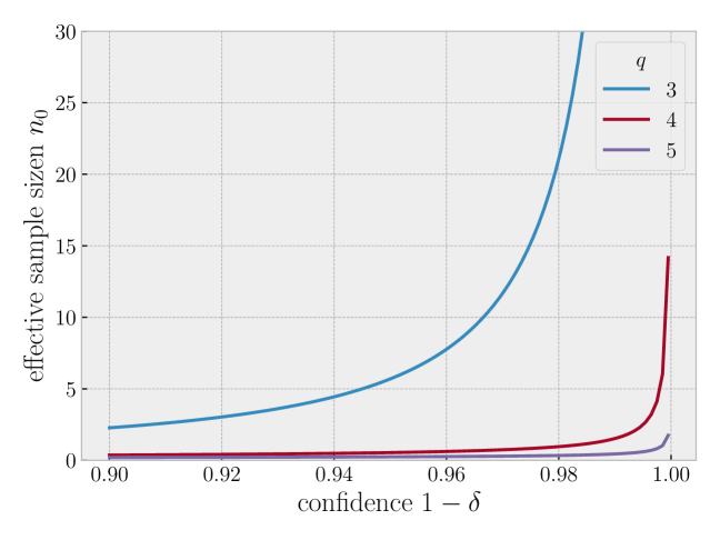
Figure 3.1: Illustration of the the effective sample size $n_{0}$ ensuring subgaussian behavior of the term $\eta(\delta,n)$ defined in (3.4) for different choices of $q$. For simplicity, we set $c_{1}=1$, $\sigma=2$ and $Q=10$.

We illustrate the behavior of $n_{0}$ depending on $1-\delta$ for different choices of $q$ in Figure 3.1 (we note that the involved constant $c_{1}$ stems from the Fuk–Nagaev inequality given in Proposition 5.1 and generally depends on $q$). We choose $c_{1}=1$ for simplicity to provide a basic intuition—note that $c_{1}$ only affects $n_{0}$ logarithmically. We refer the reader to [59] for a detailed discussion based on the bound for real-valued random variables.

Subgaussian confidence regime and convergence rates.

We now give an excess risk bound which is similar to the setting with bounded or subexponential noise: it exhibits a logarithmic dependence of the confidence parameter $\delta$ and a dependence of the sample size up to $n^{-1/3}$ depending on the level of smoothness given by $\nu$ [4, 6]. In the asymptotic large sample context, this bound is dominant and allows us to recover convergence rates.

Corollary 3.2 (Subgaussian confidence regime).

Let (MOM) and (SRC) be satisfied. Then there exist constants $\tilde{c}_{1},\tilde{c}_{2}>0$ such that with the regularization schedule

$$\alpha_{1}(n,\delta):=\tilde{c}_{2}\mathopen{}\mathclose{{\left(\frac{\log(6c_{1}/\delta)}{n}}}\right)^{\frac{1}{2\min\{\nu,1\}+1}}$$

we have

$$\lVert I_{\pi}\widehat{f}_{\alpha_{1}(n,\delta)}-f_{\star}\rVert_{L^{2}(\pi)} \leq\tilde{c}_{1}R\;\mathopen{}\mathclose{{\left(\frac{\log(6c_{1}/\delta)}{n}}}\right)^{\frac{\min\{\nu,1\}}{2\min\{\nu,1\}+1}},$$ (3.5)

with confidence $1-\delta$ for all $\delta\in D_{1}(n,q)$ and $n\in\mathbb{N}$ such that $\alpha_{1}(n,\delta)\leq\kappa^{2}$.

The constants $\tilde{c}_{1}$ and $\tilde{c}_{2}$ in Corollary 3.2 only depend on $R,\nu,\kappa,\sigma,c_{1},c_{2}$ and can be made explicit, but we omit their closed form here for the sake of a more accessible presentation. We refer the reader to the proof for more details.

Remark 3.3 (Convergence rates).

We directly obtain convergence rates from the above consideration. For fixed confidence parameter $\delta\in(0,1)$, we see that for all $n\geq n_{0}$, where $n_{0}$ is the effective sample size given in (3.4), we have $\delta\in D_{1}(n,q)$. Furthermore, there exists some $\tilde{n}_{0}\in\mathbb{N}$ such that $\alpha_{1}(n,\delta)\leq\kappa^{2}$ for all $n\geq\tilde{n}_{0}$. Combining these two insights, from Corollary 3.2, we obtain

$$\lVert I_{\pi}\widehat{f}_{\alpha_{1}(n,\delta)}-f_{\star}\rVert_{L^{2}(\pi)} \leq\tilde{c}_{1}R\;\mathopen{}\mathclose{{\left(\frac{\log(6c_{1}/\delta)}{n}}}\right)^{\frac{\min\{\nu,1\}}{2\min\{\nu,1\}+1}}$$

with confidence $1-\delta$ for all $n\geq\max\{n_{0},\tilde{n}_{0}\}$. We explicitly note that the convergence rates as well as the regularization schedule $\alpha_{1}(n,\delta)$ match exactly the known results for the capacity-independent setting that have been derived under the assumption of bounded or subexponential noise [4, 6].

Polynomial confidence regime.

By definition (3.2), the polynomial confidence regime $\delta\in D_{2}(n,q)$ is relevant in the nonasymptotic investigation whenever $n<n_{0}$. For completeness, we address this setting in Appendix B and show that Proposition 3.1 can yield simplified risk bounds with suitable regularization schedules for $\alpha$ based on $\delta$ and $n$. Depending on $\delta$, these bounds may require a stronger regularization $\alpha_{2}(n,\delta)$ than the subgaussian confidence setting. In fact, the resulting bound exhibits a polynomial worst-case dependence on $\delta$, which is compensated by a better dependence on the sample size before transitioning to the behavior from the subgaussian confidence regime given by Corollary 3.2.

4 Capacity dependent bound and optimal rates

We now improve the results from the previous section and give an excess risk bound that involves the effective dimension, which has been established as a central tool to quantify the algorithm-dependent capacity of the hypothesis space $\mathcal{H}$ relative to the distribution $\pi$ and regularization parameter $\alpha$ in order to derive risk bounds in regularized kernel-based learning under the assumptions of an eigenvalue decay of $\mathcal{C}_{\pi}$ [31, 3, 9, 10].

Definition 4.1 (Effective dimension).

For $\alpha>0$, we define

$${\mathcal{N}}(\alpha):=\operatorname{tr}\mathopen{}\mathclose{{\left({\mathcal{C}}_{\pi}({\mathcal{C}}_{\pi}+\alpha\operatorname{Id}_{\mathcal{H}})^{-1}}}\right)<\infty.$$

We now assume the standard polynomial eigenvalue decay of $\mathcal{C}_{\pi}$ [3, 9, 11].

Assumption 4.2 (Eigenvalue decay).

We assume that the nonincreasingly ordered sequence of nonzero eigenvalues $(\mu_{i})_{i\geq 1}$ of $\mathcal{T}_{\pi}$ satisfies the decay

$$\mu_{i}\leq Di^{-1/p},\quad i\in\mathbb{N}$$ (EVD)

for a constant $D>0$ and some $p\in(0,1)$.

Under the additional assumption (EVD), we can sharpen Proposition 3.1.

Proposition 4.3 (Capacity-dependent excess risk bound).

Let (MOM), (SRC) and (EVD) be satisfied. Suppose that $\delta\in(0,1)$ and

$$\log(2/\delta)\mathopen{}\mathclose{{\left(\frac{2\kappa^{2}}{n\alpha}+\frac{2\sqrt{\tilde{D}}\kappa}{\sqrt{n}\alpha^{(1+p)/2}}}}\right)\leq 1.$$ (4.1)

Then there exists a constant $c>0$ not depending on $\delta$ and $n$ such that with confidence $1-\delta$, we have

$$\|I_{\pi}\widehat{f}_{\alpha}-f_{\star}\|_{L^{2}(\pi)} \leq c\;\mathopen{}\mathclose{{\left(\alpha^{\min\{\nu,1\}}+\frac{\log(8/\delta)}{\sqrt{\alpha}n}+\sqrt{\frac{{\mathcal{N}}(\alpha)\log(8/\delta)}{n}}+\sqrt{{\mathcal{N}}(\alpha)}\cdot\eta(\delta,n,\alpha)}}\right),$$

where we set

$$\eta(\delta,n,\alpha):=\max\mathopen{}\mathclose{{\left\{\mathopen{}\mathclose{{\left(\frac{1}{\delta n^{q-1}}}}\right)^{1/q}\cdot\mathopen{}\mathclose{{\left(\frac{1}{\alpha{\mathcal{N}}(\alpha)}}}\right)^{\frac{q-2}{2q}},\sqrt{\frac{\log(8c_{1}/\delta)}{n}}}}\right\}.$$

The constant $c$ is made explicit in the proof. The key idea builds upon the original work of [3]. In particular, we incorporate the effective dimension into the Fuk–Nagaev inequality as a proxy for the $q$-th absolute moment appearing in the term $\eta(\delta,n,\alpha)$, thereby generalizing the idea to use the effective dimension as a variance proxy in the Bernstein inequality.

Corollary 4.4 (Convergence rates).

Let (MOM), (SRC) and (EVD) be satisfied. Then for every $\delta\in(0,1)$, there exists some $n_{0}\in\mathbb{N}$ such that with the regularization schedule

$$\alpha(n,\delta):=\mathopen{}\mathclose{{\left(\frac{\log(8c_{1}/\delta)}{n}}}\right)^{\frac{1}{2\min\{\nu,1\}+p}},$$

we have

$$\lVert I_{\pi}\widehat{f}_{\alpha(n,\delta)}-f_{\star}\rVert_{L^{2}(\pi)} \leq c\mathopen{}\mathclose{{\left(\frac{\log(8c_{1}/\delta)}{n}}}\right)^{\frac{\min\{\nu,1\}}{2\min\{\nu,1\}+p}}$$ (4.2)

with confidence $1-\delta$ for all $n\geq n_{0}$ with a constant $c>0$ independent of $n$ and $\delta$.

Remark 4.5 (Optimality of rates).

The rates provided by Corollary 4.4 match the rates from the literature derived for well-specified kernel ridge regression under the assumption of subexponential noise [3, 34]. In particular, these rates are known to be minimax optimal over the class of distributions satisfying (SRC), (EVD) and the Bernstein condition (1.3). Corollary 4.4 now proves that one can significantly relax the assumption of subexponential noise (1.3), as rate optimality is already achieved under the condition (MOM). Furthermore, the regularization schedule $\alpha(n,\delta)$ is the same as in the light-tailed setting—in particular, it does not depend on $q$.

5 Fuk–Nagaev inequality in Hilbert spaces

We discuss the central ingredient for the derivation of the previous results in more detail for convenience. We refer the reader to [24, 25] for the original work in the setting of real-valued random variables and [59] for a discussion of the involved constants. We present a sharpened version of a result due to [27, Theorem 3.5.1], which is formulated more generally in normed spaces, but exhibits an excess term that can be removed in the Hilbert space case. We provide the proof in Appendix C.

Proposition 5.1 (Fuk–Nagaev inequality; Hilbert space version).

Let $\xi,\xi_{1},\dots\xi_{n}$ be independent and identically distributed random variables taking values in a separable Hilbert space $\mathcal{X}$ such that

$$\mathbb{E}[\xi]=0,\quad\mathbb{E}\mathopen{}\mathclose{{\left[\lVert\xi\rVert_{\mathcal{X}}^{2}}}\right]<\sigma^{2}\quad\text{and}\quad\mathbb{E}\mathopen{}\mathclose{{\left[\lVert\xi\rVert_{\mathcal{X}}^{q}}}\right]<Q,$$

for some constants $\sigma^{2}>0$, $Q>0$ and $q\geq 3$. Write $S_{n}:=\sum_{i=1}\xi_{i}$. Then there exist two constants $c_{1}>0$ and $c_{2}>0$ depending only on $q$ such that for every $t>0$, we have

$$\mathbb{P}\mathopen{}\mathclose{{\left[\,\mathopen{}\mathclose{{\left\|\frac{1}{n}S_{n}}}\right\|_{\mathcal{X}}>t}}\right]\leq c_{1}\mathopen{}\mathclose{{\left(\frac{Q}{t^{q}n^{q-1}}+\exp\mathopen{}\mathclose{{\left(-c_{2}\frac{t^{2}n}{\sigma^{2}}}}\right)}}\right).$$ (5.1)

Remark 5.2.

For simplicity, we may assume that $1\leq c_{1}$ when we apply Proposition 5.1.

Confidence regimes.

Directly rearranging (5.1) from a tail bound to a confidence interval bound requires to solve a transcendental equation which does not admit a simple closed form solution. However, we can still derive an upper bound on the confidence intervals that reflects the superposition of polynomial and sub-gaussian tail in (5.1). By introducing

$$\delta:=2\max\mathopen{}\mathclose{{\left\{\frac{c_{1}Q}{t^{q}n^{q-1}},c_{1}\exp\mathopen{}\mathclose{{\left(-c_{2}\frac{t^{2}n}{\sigma^{2}}}}\right)}}\right\},$$ (5.2)

we have $\mathbb{P}[n^{-1}\mathopen{}\mathclose{{\left\|S_{n}}}\right\|_{\mathcal{X}}\leq t]\geq 1-\delta$ by (5.1). Rearranging (5.2), we have

$$t\geq\mathopen{}\mathclose{{\left(\frac{2c_{1}Q}{\delta n^{q-1}}}}\right)^{1/q}\quad\text{and}\quad t\geq\sigma\sqrt{\frac{\log(2c_{1}/\delta)}{c_{2}n}},$$ (5.3)

immediately leading to the following confidence bound.

Corollary 5.3 (Confidence bound).

Under the assumptions of Proposition 5.1, for all $\delta\in(0,1)$, we have

$$\mathopen{}\mathclose{{\left\|\frac{1}{n}S_{n}}}\right\|_{\mathcal{X}}\leq\max\mathopen{}\mathclose{{\left\{\mathopen{}\mathclose{{\left(\frac{2c_{1}Q}{\delta n^{q-1}}}}\right)^{1/q},\sigma\sqrt{\frac{\log(2c_{1}/\delta)}{c_{2}n}}}}\right\}$$ (5.4)

with probability at least $1-\delta$.

For every fixed $\delta$ and $n\to\infty$, this shows the typical subgaussian behavior and a convergence rate of $\frac{1}{n}S_{n}$ of the order $n^{-1/2}$ with high probability. Interpreting the right hand side as a function of $\delta$ for a fixed sample size $n$ however, the above bound characterizes a confidence regime change at $\bar{\delta}(n)$, which we define as the solution to the equation

$$\mathopen{}\mathclose{{\left(\frac{2c_{1}Q}{\bar{\delta}(n)\,n^{q-1}}}}\right)^{1/q}=\sigma\sqrt{\frac{\log(2c_{1}/\bar{\delta}(n))}{c_{2}n}}.$$ (5.5)

In fact, in the polynomial confidence regime $\delta<\bar{\delta}(n)$, the dependence of the upper bound given in Corollary 5.3 on $\delta$ is clearly worse than in the subgaussian regime $\delta\geq\bar{\delta}(n)$ which is characterized by a logarithmic dependence on $\delta$. In contrast, the polynomial confidence regime allows for a better sample dependence of $n^{-(q-1)/q}$.

Sharpness of the tail bound.

Both the subgaussian term and the polynomial term in the right hand side of the bound given by Proposition 5.1 can generally not be improved without additional assumptions. We repeat a similar argument as the one given in [60, Proposition 9], which is given in the context of linear processes. Let $\xi,\xi_{1},\dots,\xi_{n}$ be independent real-valued random variables drawn from a centered $t$-distribution with $q$ degrees of freedom, i.e. $\mathbb{E}[\xi^{q-c}]<\infty$ for all $0<c\leq q$ and let $\sigma^{2}:=\mathbb{E}[\xi^{2}]=q/(q-2)$. Then [25, Theorem 1.9] shows that we have

$$\mathbb{P}\mathopen{}\mathclose{{\left[S_{n}/n>t}}\right]=\mathbb{P}\mathopen{}\mathclose{{\left[S_{n}/\sigma>nt/\sigma}}\right]\sim 1-\phi(n^{1/2}t/\sigma)+n(1-F_{\sigma^{-1}\xi}(nt/\sigma))\quad\text{ as }n\to\infty$$

for $nt/\sigma\geq n^{1/2}$, where $\Phi$ is the standard normal cumulative distribution function and $F_{\sigma^{-1}\xi}$ is the cumulative distribution function of $\sigma^{-1}\xi$. We now note that we have the basic property $F_{\sigma^{-1}\xi}(nt/\sigma)=F_{\xi}(nt)$ and we can show that the distribution of $\xi$ satisfies $1-F(nt)\sim C_{q}/(nt)^{q}$ as $nt\to\infty$, where $C_{q}$ is a constant depending exclusively on $q$. In total, we obtain

$$\mathbb{P}\mathopen{}\mathclose{{\left[S_{n}/n>t}}\right]\sim 1-\Phi(n^{1/2}t/\sigma)+\frac{C_{q}}{t^{q}n^{q-1}}\quad\text{ as }n\to\infty$$

for $nt/\sigma\geq n^{1/2}$, showing that Proposition 5.1 is asymptotically optimal.

Appendices

The appendices are organized as follows. In Appendix A, we report all proofs of the results in the main text of this paper. In Appendix B, we provide an additional excess risk bound for the polynomial confidence regime based on Proposition 3.1. We collect some tail bounds and concentration results in Appendix C. In particular, Section C.3 contains a proof of Proposition 5.1. In Appendix D, we recall additional miscellaneous inequalities required for our proofs.

Appendix A Proofs

We provide the proofs for the results presented in the main text of this work.

A.1 Proof of Proposition 3.1

We investigate the classical bias-variance decomposition

$$I_{\pi}\widehat{f}_{\alpha}-f_{\star}=I_{\pi}\widehat{f}_{\alpha}-I_{\pi}f_{\alpha}+I_{\pi}f_{\alpha}-f_{\star}$$

and bound both terms individually.

A.1.1 Bounding the variance $I_{\pi}\widehat{f}_{\alpha}-I_{\pi}f_{\alpha}$.

We first collect some generic properties of $f_{\alpha}$. The identity $f_{\alpha}=(\mathcal{C}_{\pi}+\alpha\operatorname{Id}_{\mathcal{H}})^{-1}I_{\pi}^{*}f_{\star}$ gives

$$\mathbb{E}[\widehat{I}_{\pi}^{*}(f_{\star}-\widehat{I}_{\pi}f_{\alpha})]=I_{\pi}^{*}(f_{\star}-I_{\pi}f_{\alpha})=\alpha f_{\alpha}.$$ (A.1)

Based on (2.3), (2.4) and (2.5), we decompose the variance in $\mathcal{H}$ as

$$\widehat{f}_{\alpha}-f_{\alpha} =(\widehat{\mathcal{C}}_{\pi}+\alpha\operatorname{Id}_{\mathcal{H}})^{-1}\mathopen{}\mathclose{{\left\{\widehat{I}_{\pi}^{*}(f_{\star}-\widehat{I}_{\pi}f_{\alpha})-\alpha f_{\alpha}+\frac{1}{n}\sum_{i=1}^{n}\phi(X_{i})\varepsilon_{i}}}\right\}$$

$$=(\widehat{\mathcal{C}}_{\pi}+\alpha\operatorname{Id}_{\mathcal{H}})^{-1}\mathopen{}\mathclose{{\left\{\widehat{I}_{\pi}^{*}(f_{\star}-\widehat{I}_{\pi}f_{\alpha})-I_{\pi}^{*}(f_{\star}-I_{\pi}f_{\alpha})+\frac{1}{n}\sum_{i=1}^{n}\phi(X_{i})\varepsilon_{i}}}\right\}$$ by (A.1)

$$=(\widehat{\mathcal{C}}_{\pi}+\alpha\operatorname{Id}_{\mathcal{H}})^{-1}\mathopen{}\mathclose{{\left\{\Delta_{1}+\Delta_{2}}}\right\},$$

where we introduce the $\mathcal{H}$-valued random variables

$$\Delta_{1}=\widehat{I}_{\pi}^{*}(f_{\star}-\widehat{I}_{\pi}f_{\alpha})-\mathbb{E}[\widehat{I}_{\pi}^{*}(f_{\star}-\widehat{I}_{\pi}f_{\alpha})],\qquad\Delta_{2}=\frac{1}{n}\sum_{i=1}^{n}\phi(X_{i})\varepsilon_{i}\;.$$ (A.2)

We now obtain an $L^{2}(\pi)$-norm bound on the variance as

$$\lVert I_{\pi}(\widehat{f}_{\alpha}-f_{\alpha})\rVert_{L^{2}(\pi)} =\lVert\mathcal{C}_{\pi}^{1/2}(\widehat{f}_{\alpha}-f_{\alpha})\rVert_{\mathcal{H}}=\lVert\mathcal{C}_{\pi}^{1/2}(\widehat{\mathcal{C}}_{\pi}+\alpha\operatorname{Id}_{\mathcal{H}})^{-1}\mathopen{}\mathclose{{\left\{\Delta_{1}+\Delta_{2}}}\right\}\rVert_{\mathcal{H}}$$

$$\leq\sqrt{2}\;{\mathcal{B}}(n,\delta,\alpha)^{1/2}\mathopen{}\mathclose{{\left\|(\widehat{\mathcal{C}}_{\pi}+\alpha\operatorname{Id}_{\mathcal{H}})^{1/2}(\widehat{\mathcal{C}}_{\pi}+\alpha\operatorname{Id}_{\mathcal{H}})^{-1}\mathopen{}\mathclose{{\left\{\Delta_{1}+\Delta_{2}}}\right\}}}\right\|_{\mathcal{H}}$$

$$\leq 2\sqrt{2}\mathopen{}\mathclose{{\left\|(\widehat{\mathcal{C}}_{\pi}+\alpha\operatorname{Id}_{\mathcal{H}})^{-1/2}\mathopen{}\mathclose{{\left\{\Delta_{1}+\Delta_{2}}}\right\}}}\right\|_{\mathcal{H}}$$

$$\leq 2\sqrt{\frac{2}{\alpha}}(\lVert\Delta_{1}\rVert_{\mathcal{H}}+\lVert\Delta_{2}\rVert_{\mathcal{H}}),$$ (A.3)

with probability at least $1-\delta$, where ${\mathcal{B}}(n,\delta,\alpha)$ is defined in (C.4) and where we apply Lemma C.10 in the first inequality, Corollary C.7 in the second inequality, and additionally the fact that we have $\lVert(\widehat{\mathcal{C}}_{\pi}+\alpha\operatorname{Id}_{\mathcal{H}})^{-1/2}\rVert_{\mathcal{L}(\mathcal{H})}\leq\alpha^{-1/2}$ in the last inequality.

We now provide individual confidence bounds for $\Delta_{1}$ and $\Delta_{2}$.

Bounding $\Delta_{1}$: Bennett inequality.

We introduce the independent and identically distributed random variables $\xi_{i}:=(f_{\star}(X_{i})-f_{\alpha}(X_{i}))\phi(X_{i})\in\mathcal{H}$ and note that $\Delta_{1}:=\frac{1}{n}\sum_{i=1}^{n}(\xi_{i}-\mathbb{E}[\xi_{i}])$ and proceed similarly as in the proof of [4, Theorem 1 & Theorem 5].

To apply Bennett’s inequality, we need to bound the norm of the $\xi_{i}$. First, note that almost surely, we have by (SRC), for some $f\in L^{2}(\pi)$, such that $\lVert f\rVert_{L^{2}(\pi)}\leq R$

$$\lVert f_{\alpha}(X_{i})\phi(X_{i})\rVert_{{\mathcal{H}}} =\lVert\langle f_{\alpha},\phi(X_{i})\rangle_{{\mathcal{H}}}\phi(X_{i})\rVert_{{\mathcal{H}}}$$

$$\leq\kappa^{2}\|f_{\alpha}\|_{\mathcal{H}}$$

$$=\kappa^{2}\|({\mathcal{C}}_{\pi}+\alpha\operatorname{Id}_{{\mathcal{H}}})^{-1}I_{\pi}^{*}f_{\star}\|_{\mathcal{H}}$$

$$=\kappa^{2}\|I_{\pi}^{*}({\mathcal{T}}_{\pi}+\alpha\operatorname{Id}_{{\mathcal{H}}})^{-1}{\mathcal{T}}_{\pi}^{\nu}f\|_{\mathcal{H}}.$$

A short calculation shows that for $\nu\geq 1/2$, the map $h(t)=t^{\nu+1/2}(t+\alpha)^{-1}$ is increasing on the spectrum of ${\mathcal{T}}_{\pi}$ with

$$\sup_{t\in(0,\kappa^{2}]}|h(t)|=\sup_{t\in(0,\kappa^{2}]}t^{\nu-1/2}\frac{t}{t+\alpha}\leq\kappa^{2(\nu-1/2)},$$

for all $\alpha>0$. Hence,

$$\|I_{\pi}^{*}({\mathcal{T}}_{\pi}+\alpha\operatorname{Id}_{{\mathcal{H}}})^{-1}{\mathcal{T}}_{\pi}^{\nu}f\|_{\mathcal{H}}\leq R\cdot\sup_{t\in(0,\kappa^{2}]}|h(t)|\leq R\cdot\kappa^{2(\nu-1/2)}$$

and therefore

$$\lVert f_{\alpha}(X_{i})\phi(X_{i})\rVert_{{\mathcal{H}}}\leq R\cdot\kappa^{2\nu+1}\;.$$

This gives

$$\lVert\xi_{i}\rVert_{\mathcal{H}} \leq\kappa\lVert f_{\star}\rVert_{L^{\infty}(\pi)}+\lVert f_{\alpha}(X_{i})\phi(X_{i})\rVert_{{\mathcal{H}}}$$

$$\leq\kappa\lVert f_{\star}\rVert_{L^{\infty}(\pi)}+R\cdot\kappa^{2\nu+1}.$$

Furthermore, by [61, Proposition 3.3] and [11, Lemma 25] we see

$$\mathbb{E}[\lVert\xi_{i}\rVert^{2}_{\mathcal{H}}] \leq\kappa^{2}\lVert f_{\star}-I_{\pi}f_{\alpha}\rVert^{2}_{L^{2}(\pi)}$$

$$=\kappa^{2}\lVert(\operatorname{Id}_{{\mathcal{H}}}-{\mathcal{T}}_{\pi}({\mathcal{T}}_{\pi}+\alpha\operatorname{Id}_{{\mathcal{H}}})^{-1}){\mathcal{T}}_{\pi}^{\nu}f\rVert^{2}_{L^{2}(\pi)}$$

$$\leq\kappa^{2}R^{2}\alpha^{2\min\{\nu,1\}}.$$

Applying Proposition C.2 to $\Delta_{1}=\frac{1}{n}\sum_{i=1}^{n}(\xi_{i}-\mathbb{E}[\xi_{i}])$, with probability at least $1-\delta$ for for any $1>\delta>0$, we have

$$\lVert\Delta_{1}\rVert_{\mathcal{H}} \leq\frac{2(\kappa\lVert f_{\star}\rVert_{L^{\infty}(\pi)}+R\cdot\kappa^{2\nu+1})\log(2/\delta)}{n}+\sqrt{\frac{2\kappa^{2}R^{2}\alpha^{2\min\{\nu,1\}}\log(2/\delta)}{n}}$$

$$\leq\tilde{C}_{\diamond}\cdot\mathopen{}\mathclose{{\left(\frac{\log(2/\delta)}{n}+\sqrt{\frac{\alpha^{2\min\{\nu,1\}}\log(2/\delta)}{n}}}}\right),$$ (A.4)

where we use $\sqrt{2\log(2/\delta)}\leq 2\log(2/\delta)$ and with

$$\tilde{C}_{\diamond}=2\kappa\cdot\max\{\lVert f_{\star}\rVert_{L^{\infty}(\pi)}+R\cdot\kappa^{2\nu},R\}.$$ (A.5)

Bounding $\Delta_{2}$: Fuk–Nagaev inequality.

We introduce the independent and identically distributed random variables $\zeta_{i}:=\phi(X_{i})\varepsilon_{i}$ and note that $\Delta_{2}=\frac{1}{n}\sum_{i=1}^{n}\zeta_{i}$. By 2.2, we clearly have $\mathbb{E}[\zeta_{i}]=\mathbb{E}\mathopen{}\mathclose{{\left[\phi(X_{i})\mathbb{E}[\varepsilon_{i}\mid X]}}\right]=0$ as well as

$$\mathbb{E}[\lVert\zeta_{i}\rVert^{2}_{\mathcal{H}}]<\kappa^{2}\sigma^{2}\quad\text{and}\quad\mathbb{E}[\lVert\zeta_{i}\rVert^{q}_{\mathcal{H}}]<\kappa^{q}Q.$$

We can therefore apply Corollary 5.3 to $\Delta_{2}=\frac{1}{n}\sum_{i=1}^{n}\zeta_{i}$ and obtain

$$\mathopen{}\mathclose{{\left\|\Delta_{2}}}\right\|_{\mathcal{H}}\leq\max\mathopen{}\mathclose{{\left\{\mathopen{}\mathclose{{\left(\frac{2c_{1}\kappa^{q}Q}{\delta n^{q-1}}}}\right)^{1/q},\kappa\sigma\;\sqrt{\frac{\log(2c_{1}/\delta)}{c_{2}n}}}}\right\}$$ (A.6)

with probability at least $1-\delta$.

Collecting the terms.

By the union bound, the three individual confidence bounds (A.3), (A.1.1) and (A.6) and hold simultaneously with probability at least $1-\delta$. We have

$$\lVert I_{\pi}(\widehat{f}_{\alpha}-f_{\alpha})\rVert_{L^{2}(\pi)} \leq\frac{C_{\diamond}}{\sqrt{\alpha}}\mathopen{}\mathclose{{\left(\frac{\log(6/\delta)}{n}+\sqrt{\frac{\alpha^{2\min\{\nu,1\}}\log(6/\delta)}{n}}+\eta(\delta,n)}}\right).$$

Here, we set

$$\eta(\delta,n):=\max\mathopen{}\mathclose{{\left\{\mathopen{}\mathclose{{\left(\frac{Q}{\delta n^{q-1}}}}\right)^{1/q},\sigma\;\sqrt{\frac{\log(6c_{1}/\delta)}{n}}}}\right\}$$

and

$$C_{\diamond}=2\sqrt{2}\max\{\tilde{C}_{\diamond},\kappa\cdot\max\{(6c_{1})^{1/q},1/\sqrt{c_{2}}\}\}.$$ (A.7)

A.1.2 Bounding the bias $I_{\pi}f_{\alpha}-f_{\star}$

We apply the standard theory of source conditions in inverse problems as discussed for example by [55]. In particular, under the $L^{2}(\pi)$-source condition given by (SRC), we have

$$\lVert I_{\pi}f_{\alpha}-f_{\star}\rVert_{L^{2}(\pi)}\leq R\alpha^{\min\{\nu,1\}},$$

see e.g. [61, Proposition 3.3]. Combining the variance bound and the bias bound yields the result.

A.2 Proof of Corollary 3.2

Let $\delta\in D_{1}(n,q)$. Using that $\alpha\leq\kappa^{2}$ and recalling that $c_{1}\geq 1$, we find by Proposition 3.1 for any $\delta\in D_{1}(n,q)$ with confidence $1-\delta$

$$\lVert I_{\pi}(\widehat{f}_{\alpha}-f_{\star})\rVert_{L^{2}(\pi)} \leq R\alpha^{\min\{\nu,1\}}+\frac{C_{\diamond}}{\sqrt{\alpha}}\mathopen{}\mathclose{{\left(\frac{\log(6/\delta)}{n}+\sqrt{\frac{\alpha^{2\min\{\nu,1\}}\log(6/\delta)}{n}}+\sigma\sqrt{\frac{\log(6c_{1}/\delta)}{n}}}}\right).$$

Assuming

$$\alpha^{\min\{\nu,1\}}\sqrt{n}\geq\sqrt{\log(6/\delta)}$$ (A.8)

gives

$$\frac{\log(6/\delta)}{n}\leq\sqrt{\frac{\alpha^{2\min\{\nu,1\}}\log(6/\delta)}{n}}\leq\kappa^{2\min\{\nu,1\}}\sqrt{\frac{\log(6c_{1}/\delta)}{n}}.$$

Hence,

$$\lVert I_{\pi}\widehat{f}_{\alpha}-f_{\star}\rVert_{L^{2}(\pi)} \leq R\alpha^{\min\{\nu,1\}}+c_{3}\sqrt{\frac{\log(6c_{1}/\delta)}{\alpha n}},$$

with $c_{3}=3C_{\diamond}\max\{\kappa^{2\min\{\nu,1\}},\sigma\}$. Ensuring that the remaining estimation error contribution will not be dominated by the approximation error, we see that the regularization parameter has to satisfy

$$\alpha\geq c_{4}\;\mathopen{}\mathclose{{\left(\frac{\log(6c_{1}/\delta)}{n}}}\right)^{\frac{1}{2\min\{\nu,1\}+1}},$$ (A.9)

with $c_{4}=(c_{3}/R)^{\frac{1}{\min\{\nu,1\}+1/2}}$. We therefore obtain

$$\lVert I_{\pi}\widehat{f}_{\alpha}-f_{\star}\rVert_{L^{2}(\pi)} \leq\tilde{c}_{1}R\;\mathopen{}\mathclose{{\left(\frac{\log(6c_{1}/\delta)}{n}}}\right)^{\frac{\min\{\nu,1\}}{2\min\{\nu,1\}+1}},$$

with confidence $1-\delta$ and $\tilde{c}_{1}=2c_{4}^{\min\{\nu,1\}}$. In order for this bound to hold, the regularization strength has to fulfill condition (3.1), (A.8) and (A.9), that is,

$$\alpha\geq\max\mathopen{}\mathclose{{\left\{c_{4}\mathopen{}\mathclose{{\left(\frac{\log(6c_{1}/\delta)}{n}}}\right)^{\frac{1}{2\min\{\nu,1\}+1}},\mathopen{}\mathclose{{\left(\frac{\log(6/\delta)}{n}}}\right)^{\frac{1}{2\min\{\nu,1\}}},C_{\kappa}\frac{\log(6/\delta)}{\sqrt{n}}}}\right\}$$ (A.10)

in addition to the restriction $\alpha\leq\kappa^{2}$. As we always have $n^{-\frac{1}{2\min\{\nu,1\}}}\leq n^{-1/2}\leq n^{-\frac{1}{2\min\{\nu,1\}+1}}$ for $\nu\geq 1/2$ and $\log(6c_{1}/\delta)\geq\log(6/\delta)$, there exists a constant $\tilde{c}_{2}$ such that

$$\alpha_{1}(n,\delta):=\tilde{c}_{2}\mathopen{}\mathclose{{\left(\frac{\log(6c_{1}/\delta)}{n}}}\right)^{\frac{1}{2\min\{\nu,1\}+1}}$$

satisfies (A.10).

A.3 Proof of Proposition 4.3

We split again into variance and bias:

$$I_{\pi}\widehat{f}_{\alpha}-f_{\star}=I_{\pi}(\widehat{f}_{\alpha}-f_{\alpha})+I_{\pi}f_{\alpha}-f_{\star}.$$

A.3.1 Bounding the variance $I_{\pi}\widehat{f}_{\alpha}-I_{\pi}f_{\alpha}$

Following [62, Appendix C], we further decompose the variance term in $L^{2}(\pi)$ as

$$I_{\pi}\widehat{f}_{\alpha}-I_{\pi}f_{\alpha} =I_{\pi}\widehat{f}_{\alpha}-I_{\pi}\widehat{\mathcal{C}}_{\pi}(\widehat{\mathcal{C}}_{\pi}+\alpha\operatorname{Id}_{\mathcal{H}})^{-1}f_{\alpha}+I_{\pi}\widehat{\mathcal{C}}_{\pi}(\widehat{\mathcal{C}}_{\pi}+\alpha\operatorname{Id}_{\mathcal{H}})^{-1}f_{\alpha}-I_{\pi}f_{\alpha}$$

$$=\underbrace{I_{\pi}(\widehat{\mathcal{C}}_{\pi}+\alpha\operatorname{Id}_{\mathcal{H}})^{-1}\mathopen{}\mathclose{{\left(\widehat{\Upsilon}-\widehat{\mathcal{C}}_{\pi}f_{\alpha}}}\right)}_{=:I_{1}}+\underbrace{\alpha I_{\pi}(\widehat{\mathcal{C}}_{\pi}+\alpha\operatorname{Id}_{\mathcal{H}})^{-1}f_{\alpha}}_{=:I_{2}},$$ (A.11)

where we use the definition of $\widehat{f}_{\alpha}$ in (2.4) for the first term and the identity

$$\widehat{\mathcal{C}}_{\pi}(\widehat{\mathcal{C}}_{\pi}+\alpha\operatorname{Id}_{\mathcal{H}})^{-1}-\operatorname{Id}_{\mathcal{H}}=\alpha(\widehat{\mathcal{C}}_{\pi}+\alpha\operatorname{Id}_{\mathcal{H}})^{-1}$$

for the second summand.

A.3.2 Bounding the first term $I_{1}$

We introduce the shorthand notation ${\mathcal{C}}_{\alpha}:=\mathcal{C}_{\pi}+\alpha\operatorname{Id}_{\mathcal{H}}$, $\widehat{{\mathcal{C}}}_{\alpha}:=\widehat{\mathcal{C}}_{\pi}+\alpha\operatorname{Id}_{\mathcal{H}}$. We note that we may write

$$\mathcal{C}_{\pi}^{1/2}(\widehat{\mathcal{C}}_{\pi}+\alpha\operatorname{Id}_{\mathcal{H}})^{-1} =\mathcal{C}_{\pi}^{1/2}{\mathcal{C}}_{\alpha}^{-1/2}{\mathcal{C}}_{\alpha}^{1/2}\widehat{{\mathcal{C}}}_{\alpha}^{-1/2}\widehat{{\mathcal{C}}}_{\alpha}^{-1/2}{\mathcal{C}}_{\alpha}^{1/2}{\mathcal{C}}_{\alpha}^{-1/2}.$$

Recall that $\|\mathcal{C}_{\pi}^{1/2}{\mathcal{C}}_{\alpha}^{-1/2}\|_{{\mathcal{L}}({\mathcal{H}})}\leq 1$ and that by Corollary C.9 and Lemma D.2, with confidence $1-\delta$, we have

$$\|{\mathcal{C}}_{\alpha}^{1/2}\widehat{{\mathcal{C}}}_{\alpha}^{-1/2}\|_{{\mathcal{L}}({\mathcal{H}})}=\|\widehat{{\mathcal{C}}}_{\alpha}^{-1/2}{\mathcal{C}}_{\alpha}^{1/2}\|_{{\mathcal{L}}({\mathcal{H}})}\leq 2,$$

provided (4.1) is satisfied. Hence, by (2.1), with confidence $1-\delta$

$$\|I_{1}\|_{L^{2}(\pi)}=\lVert I_{\pi}(\widehat{\mathcal{C}}_{\pi}+\alpha\operatorname{Id}_{\mathcal{H}})^{-1}(\widehat{\Upsilon}-\widehat{\mathcal{C}}_{\pi}f_{\alpha})\rVert_{L^{2}(\pi)} \leq 4\;\lVert(\mathcal{C}_{\pi}+\alpha\operatorname{Id}_{\mathcal{H}})^{-1/2}(\widehat{\Upsilon}-\widehat{\mathcal{C}}_{\pi}f_{\alpha})\rVert_{\mathcal{H}}.$$ (A.12)

We proceed by further splitting

$$(\mathcal{C}_{\pi}+\alpha\operatorname{Id}_{\mathcal{H}})^{-1/2}(\widehat{\Upsilon}-\widehat{\mathcal{C}}_{\pi}f_{\alpha}) =(\mathcal{C}_{\pi}+\alpha\operatorname{Id}_{\mathcal{H}})^{-1/2}[(\widehat{\Upsilon}-\widehat{\mathcal{C}}_{\pi}f_{\alpha})-(I_{\pi}^{*}f_{\star}-\mathcal{C}_{\pi}f_{\alpha})]$$

$$\quad+(\mathcal{C}_{\pi}+\alpha\operatorname{Id}_{\mathcal{H}})^{-1/2}(I_{\pi}^{*}f_{\star}-\mathcal{C}_{\pi}f_{\alpha}).$$

Note that by (2.5), we have

$$\widehat{\Upsilon}=\widehat{I}_{\pi}^{*}f_{\star}+\frac{1}{n}\sum_{i=1}^{n}\phi(X_{i})\varepsilon_{i}.$$

Introducing

$$\Delta_{1}:=(\widehat{I}_{\pi}^{*}f_{\star}-\widehat{\mathcal{C}}_{\pi}f_{\alpha})-(I_{\pi}^{*}f_{\star}-\mathcal{C}_{\pi}f_{\alpha}),\qquad\Delta_{2}:=\frac{1}{n}\sum_{i=1}^{n}\phi(X_{i})\varepsilon_{i},$$

we obtain

$$(\mathcal{C}_{\pi}+\alpha\operatorname{Id}_{\mathcal{H}})^{-1/2}(\widehat{\Upsilon}-\widehat{\mathcal{C}}_{\pi}f_{\alpha}) =I_{11}+I_{12}+I_{13},$$

where we set

$$I_{11} :=(\mathcal{C}_{\pi}+\alpha\operatorname{Id}_{\mathcal{H}})^{-1/2}\Delta_{1}$$

$$I_{12} :=(\mathcal{C}_{\pi}+\alpha\operatorname{Id}_{\mathcal{H}})^{-1/2}\Delta_{2}$$

$$I_{13} :=(\mathcal{C}_{\pi}+\alpha\operatorname{Id}_{\mathcal{H}})^{-1/2}(I_{\pi}^{*}f_{\star}-\mathcal{C}_{\pi}f_{\alpha}).$$

Thus, with (A.12), we have

$$\|I_{1}\|_{L^{2}(\pi)}\leq 4\mathopen{}\mathclose{{\left(\|I_{11}\|_{\mathcal{H}}+\|I_{12}\|_{\mathcal{H}}+\|I_{13}\|_{\mathcal{H}}}}\right)$$ (A.13)

We proceed to bound the terms on the right hand side individually.

Bounding $\|I_{11}\|_{\mathcal{H}}$.

To bound the norm of $I_{11}$, we apply Bennett’s inequality Proposition C.2 to the independent and identically distributed random variables

$$\xi_{i}:=(\mathcal{C}_{\pi}+\alpha\operatorname{Id}_{\mathcal{H}})^{-1/2}(f_{\star}(X_{i})-f_{\alpha}(X_{i}))\phi(X_{i}).$$

Then

$$I_{11}=\frac{1}{n}\sum_{i=1}^{n}\xi_{i}-\mathbb{E}[\xi_{i}].$$

Furthermore,

$$\mathbb{E}[\|\xi_{i}\|^{2}_{\mathcal{H}}] \leq\sup_{X\in\mathcal{X}}|f_{\star}(X)-f_{\alpha}(X)|^{2}\;\mathbb{E}[\|(\mathcal{C}_{\pi}+\alpha\operatorname{Id}_{\mathcal{H}})^{-1/2}\phi(X_{i})\|^{2}_{\mathcal{H}}].$$

since $f_{\alpha}\in{\mathcal{H}}$ and by (SRC), we have for $\nu\geq 1/2$

$$|f_{\alpha}(X)| =|\langle f_{\alpha},\phi(X)\rangle_{{\mathcal{H}}}|$$

$$=|\langle(\mathcal{C}_{\pi}+\alpha\operatorname{Id}_{\mathcal{H}})^{-1}I_{\pi}^{*}{\mathcal{T}}_{\pi}^{\nu}f,\phi(X)\rangle_{{\mathcal{H}}}|$$

$$=|\langle f,{\mathcal{T}}_{\pi}^{\nu}I_{\pi}(\mathcal{C}_{\pi}+\alpha\operatorname{Id}_{\mathcal{H}})^{-1}\phi(X)\rangle_{L^{2}(\pi)}|$$

$$\leq\kappa R\|I_{\pi}^{*}({\mathcal{T}}_{\pi}+\alpha\operatorname{Id}_{L^{2}(\pi)})^{-1}{\mathcal{T}}_{\pi}^{\nu}\|_{{\mathcal{L}}(L^{2}(\pi),\mathcal{H})}$$

$$\leq\kappa R\sup_{0<t\leq\kappa^{2}}|t^{\nu+1/2}(t+\alpha)^{-1}|$$

$$\leq\kappa^{2\nu}R.$$ (A.14)

We proceed with writing

$$\mathbb{E}[\|(\mathcal{C}_{\pi}+\alpha\operatorname{Id}_{\mathcal{H}})^{-1/2}\phi(X_{i})\|^{2}_{\mathcal{H}}] =\mathbb{E}[\operatorname{tr}((\mathcal{C}_{\pi}+\alpha\operatorname{Id}_{\mathcal{H}})^{-1}\phi(X_{i})\otimes\phi(X_{i}))]={\mathcal{N}}(\alpha).$$

Hence,

$$\mathbb{E}[\|\xi_{i}\|^{2}_{\mathcal{H}}] \leq 2(\|f_{\star}\|^{2}_{\infty}+\kappa^{4\nu}R^{2}){\mathcal{N}}(\alpha)=:\tilde{\sigma}^{2}.$$

Moreover,

$$\|\xi_{i}\|_{\mathcal{H}} =\|(\mathcal{C}_{\pi}+\alpha\operatorname{Id}_{\mathcal{H}})^{-1/2}(f_{\star}(X_{i})-f_{\alpha}(X_{i}))\phi(X_{i})\|_{\mathcal{H}}$$

$$\leq\|f_{\star}(X_{i})(\mathcal{C}_{\pi}+\alpha\operatorname{Id}_{\mathcal{H}})^{-1/2}\phi(X_{i})\|_{\mathcal{H}}+\|f_{\alpha}(X_{i})(\mathcal{C}_{\pi}+\alpha\operatorname{Id}_{\mathcal{H}})^{-1/2}\phi(X_{i})\|_{\mathcal{H}}$$

$$\leq\frac{\kappa\|f_{\star}\|_{\infty}}{\sqrt{\alpha}}+\frac{\kappa f_{\alpha}(X_{i})}{\sqrt{\alpha}}$$

$$\leq\frac{\kappa}{\sqrt{\alpha}}\;(\|f_{\star}\|_{\infty}+\kappa^{2\nu}R)=:L.$$

In the last step we use (A.3.2). From Proposition C.2, we obtain with confidence $1-\delta$

$$\|I_{11}\|_{\mathcal{H}} \leq\frac{2L\log(2/\delta)}{n}+\sqrt{\frac{2\tilde{\sigma}^{2}\log(2/\delta)}{n}}$$

$$\leq c_{11}\mathopen{}\mathclose{{\left(\frac{\log(2/\delta)}{\sqrt{\alpha}n}+\sqrt{\frac{{\mathcal{N}}(\alpha)\log(2/\delta)}{n}}}}\right),$$ (A.15)

with $c_{11}=2(\|f_{\star}\|_{\infty}+\kappa^{2\nu}R)\;\max\{1,\kappa\}$.

Bounding $\|I_{12}\|_{\mathcal{H}}$.

The idea is to apply the Fuk-Nagaev inequality Corollary 5.3 to the independent and identically distributed random variables

$$\zeta_{i}:=\varepsilon_{i}(\mathcal{C}_{\pi}+\alpha\operatorname{Id}_{\mathcal{H}})^{-1/2}\phi(X_{i}).$$

We repeatedly apply 2.2 to bound the expectation and moments of the $\zeta_{i}$. We get

$$\mathbb{E}[\zeta_{i}] =\mathbb{E}[\underbrace{\mathbb{E}[\varepsilon_{i}|X_{i}]}_{=0}(\mathcal{C}_{\pi}+\alpha\operatorname{Id}_{\mathcal{H}})^{-1/2}\phi(X_{i})]=0.$$

Moreover,

$$\mathbb{E}[\|\zeta_{i}\|^{2}_{\mathcal{H}}] =\mathbb{E}[\mathbb{E}[\varepsilon^{2}_{i}|X_{i}]\;\|(\mathcal{C}_{\pi}+\alpha\operatorname{Id}_{\mathcal{H}})^{-1/2}\phi(X_{i})\|^{2}_{\mathcal{H}}]$$

$$<\sigma^{2}\mathbb{E}[\operatorname{tr}((\mathcal{C}_{\pi}+\alpha\operatorname{Id}_{\mathcal{H}})^{-1}\phi(X_{i})\otimes\phi(X_{i}))]$$

$$=\sigma^{2}{\mathcal{N}}(\alpha)$$

$$=:\tilde{\sigma}^{2}.$$

Since $q>2$, we find

$$\mathbb{E}[\|\zeta_{i}\|^{q}_{\mathcal{H}}] =\mathbb{E}[\mathbb{E}[|\varepsilon_{i}|^{q}|X_{i}]\;\|(\mathcal{C}_{\pi}+\alpha\operatorname{Id}_{\mathcal{H}})^{-1/2}\phi(X_{i})\|^{q}_{\mathcal{H}}]$$

$$<Q\;\mathbb{E}[\|(\mathcal{C}_{\pi}+\alpha\operatorname{Id}_{\mathcal{H}})^{-1/2}\phi(X_{i})\|^{2}_{\mathcal{H}}\|(\mathcal{C}_{\pi}+\alpha\operatorname{Id}_{\mathcal{H}})^{-1/2}\phi(X_{i})\|^{q-2}_{\mathcal{H}}]$$

$$\leq Q\;\kappa^{q-2}\mathopen{}\mathclose{{\left(\frac{1}{\alpha}}}\right)^{\frac{q-2}{2}}{\mathcal{N}}(\alpha)$$

$$=:\tilde{Q}.$$

Since $\frac{1}{n}\sum_{i=1}^{n}\zeta_{i}=I_{12}$, applying Corollary 5.3 gives with confidence $1-\delta$

$$\|I_{12}\|_{\mathcal{H}} \leq\max\mathopen{}\mathclose{{\left\{\mathopen{}\mathclose{{\left(\frac{2c_{1}\tilde{Q}}{\delta n^{q-1}}}}\right)^{1/q},\tilde{\sigma}\;\sqrt{\frac{\log(2c_{1}/\delta)}{c_{2}n}}}}\right\}$$

$$=\max\mathopen{}\mathclose{{\left\{\mathopen{}\mathclose{{\left(\frac{2c_{1}\kappa^{q-2}Q}{\delta n^{q-1}}}}\right)^{1/q}\mathopen{}\mathclose{{\left(\frac{1}{\alpha}}}\right)^{\frac{q-2}{2q}}{\mathcal{N}}(\alpha)^{1/q},\sigma\;\sqrt{\frac{{\mathcal{N}}(\alpha)\log(2c_{1}/\delta)}{c_{2}n}}}}\right\}$$

$$\leq c_{12}\sqrt{{\mathcal{N}}(\alpha)}\;\max\mathopen{}\mathclose{{\left\{\mathopen{}\mathclose{{\left(\frac{1}{\delta n^{q-1}}}}\right)^{1/q}\mathopen{}\mathclose{{\left(\frac{1}{\alpha{\mathcal{N}}(\alpha)}}}\right)^{\frac{q-2}{2q}},\sqrt{\frac{\log(2c_{1}/\delta)}{n}}}}\right\},$$ (A.16)

with $c_{12}=\max\{(2c_{1}\kappa^{q-2}Q)^{1/q},\sigma/\sqrt{c_{2}}\}$.

Bounding $\|I_{13}\|_{\mathcal{H}}$.

Using the definition of $f_{\alpha}$ from (2.3), we see that by (SRC), we have

$$I_{13} =(\mathcal{C}_{\pi}+\alpha\operatorname{Id}_{\mathcal{H}})^{-1/2}(I_{\pi}^{*}f_{\star}-\mathcal{C}_{\pi}(\mathcal{C}_{\pi}+\alpha\operatorname{Id}_{\mathcal{H}})^{-1}I_{\pi}^{*}f_{\star})$$

$$=(\mathcal{C}_{\pi}+\alpha\operatorname{Id}_{\mathcal{H}})^{-1/2}(\operatorname{Id}_{\mathcal{H}}-\mathcal{C}_{\pi}(\mathcal{C}_{\pi}+\alpha\operatorname{Id}_{\mathcal{H}})^{-1})I_{\pi}^{*}f_{\star}$$

$$=(\mathcal{C}_{\pi}+\alpha\operatorname{Id}_{\mathcal{H}})^{-1/2}(\operatorname{Id}_{\mathcal{H}}-\mathcal{C}_{\pi}(\mathcal{C}_{\pi}+\alpha\operatorname{Id}_{\mathcal{H}})^{-1})I_{\pi}^{*}{\mathcal{T}}_{\pi}^{\nu}f$$

$$=I_{\pi}^{*}({\mathcal{T}}_{\pi}+\alpha\operatorname{Id}_{L^{2}})^{-1/2}(\operatorname{Id}_{L^{2}}-{\mathcal{T}}_{\pi}({\mathcal{T}}_{\pi}+\alpha\operatorname{Id}_{L^{2}})^{-1}){\mathcal{T}}_{\pi}^{\nu}f$$

$$=\tilde{U}{\mathcal{T}}_{\pi}^{1/2}({\mathcal{T}}_{\pi}+\alpha\operatorname{Id}_{L^{2}})^{-1/2}(\operatorname{Id}_{L^{2}}-{\mathcal{T}}_{\pi}({\mathcal{T}}_{\pi}+\alpha\operatorname{Id}_{L^{2}})^{-1}){\mathcal{T}}_{\pi}^{\nu}f,$$

for some $f\in L^{2}(\pi)$ satisfying $\|f\|_{L^{2}(\pi)}\leq R$ and the partial isometry $\tilde{U}:L^{2}(\pi)\to\mathcal{H}$ given by (2.1). This gives

$$\|I_{13}\|_{{\mathcal{H}}} \leq R\sup_{0<t\leq\kappa^{2}}|\alpha t^{\nu+1/2}(t+\alpha)^{-3/2}|$$

$$\leq R\sup_{0<t\leq\kappa^{2}}|\alpha t^{\nu}(t+\alpha)^{-1}|\sup_{0<t\leq\kappa^{2}}|t^{1/2}(t+\alpha)^{-1/2}|$$

$$\leq R\sup_{0<t\leq\kappa^{2}}|\alpha t^{\nu}(t+\alpha)^{-1}|$$

$$\leq R\max\{1,{\kappa^{2(\nu-1)}}\}\,\alpha^{\min\{\nu,1\}}=c_{13}\,\alpha^{\min\{\nu,1\}},$$ (A.17)

where we use Lemma D.1 for the last inequality and set $c_{13}:=R\max\{1,{\kappa^{2(\nu-1)}}\}$.

Collecting all terms.

Collecting the bounds (A.3.2), (A.3.2), (A.3.2), together with (A.13) and taking a union bound gives with confidence $1-\delta$

$$\|I_{1}\|_{L^{2}(\pi)} \leq 4\mathopen{}\mathclose{{\left(\|I_{11}\|_{\mathcal{H}}+\|I_{12}\|_{\mathcal{H}}+\|I_{13}\|_{\mathcal{H}}}}\right)$$

$$\leq c_{\kappa,\nu,q,R}\;\mathopen{}\mathclose{{\left(\alpha^{\min\{\nu,1\}}+\frac{\log(4/\delta)}{\sqrt{\alpha}n}+\sqrt{\frac{{\mathcal{N}}(\alpha)\log(4/\delta)}{n}}+\sqrt{{\mathcal{N}}(\alpha)}\cdot\eta(\delta,n,\alpha)}}\right),$$ (A.18)

where we set

$$\eta(\delta,n,\alpha):=\max\mathopen{}\mathclose{{\left\{\mathopen{}\mathclose{{\left(\frac{1}{\delta n^{q-1}}}}\right)^{1/q}\mathopen{}\mathclose{{\left(\frac{1}{\alpha{\mathcal{N}}(\alpha)}}}\right)^{\frac{q-2}{2q}},\sqrt{\frac{\log(4c_{1}/\delta)}{n}}}}\right\},$$

and with $c_{\kappa,\nu,q,R}:=4\max\{c_{11},c_{12},c_{13}\}$.

A.3.3 Bounding the second term $I_{2}$

We write again ${\mathcal{C}}_{\alpha}:=\mathcal{C}_{\pi}+\alpha\operatorname{Id}_{\mathcal{H}}$, $\widehat{{\mathcal{C}}}_{\alpha}:=\widehat{\mathcal{C}}_{\pi}+\alpha\operatorname{Id}_{\mathcal{H}}$ and find with Lemma D.2 and Corollary C.9 with confidence $1-\delta$

$$\|I_{2}\|_{L^{2}(\pi)} =\|\alpha I_{\pi}(\widehat{\mathcal{C}}_{\pi}+\alpha\operatorname{Id}_{\mathcal{H}})^{-1}f_{\alpha}\|_{L^{2}(\pi)}$$

$$=\alpha\|I_{\pi}{\mathcal{C}}_{\alpha}^{-1/2}{\mathcal{C}}_{\alpha}^{1/2}\widehat{{\mathcal{C}}}_{\alpha}^{-1/2}\widehat{{\mathcal{C}}}_{\alpha}^{-1/2}{\mathcal{C}}_{\alpha}^{1/2}{\mathcal{C}}_{\alpha}^{-1/2}f_{\alpha}\|_{L^{2}(\pi)}$$

$$=\alpha\|{\mathcal{C}}_{\pi}^{1/2}{\mathcal{C}}_{\alpha}^{-1/2}{\mathcal{C}}_{\alpha}^{1/2}\widehat{{\mathcal{C}}}_{\alpha}^{-1/2}\widehat{{\mathcal{C}}}_{\alpha}^{-1/2}{\mathcal{C}}_{\alpha}^{1/2}{\mathcal{C}}_{\alpha}^{-1/2}f_{\alpha}\|_{\mathcal{H}}$$

$$\leq 4\alpha\;\|{\mathcal{C}}_{\alpha}^{-1/2}f_{\alpha}\|_{\mathcal{H}},$$

where we again use (2.1) and $\|\mathcal{C}_{\pi}^{1/2}{\mathcal{C}}_{\alpha}^{-1/2}\|_{{\mathcal{L}}({\mathcal{H}})}\leq 1$. Hence, by (SRC) and the definition of $f_{\alpha}$, we have with confidence $1-\delta$

$$\|I_{2}\|_{L^{2}(\pi)} \leq 4\alpha\;\|{\mathcal{C}}_{\alpha}^{-1/2}f_{\alpha}\|_{\mathcal{H}}$$

$$\leq 4R\sup_{0<t\leq\kappa^{2}}|\alpha(t+\alpha)^{-3/2}t^{\nu+1/2}|$$

$$\leq 4R\max\{1,{\kappa^{2(\nu-1)}}\}\,\alpha^{\min\{\nu,1\}}=4c_{13}\,\alpha^{\min\{\nu,1\}},$$ (A.19)

where we repeat the computation from (A.3.2).

A.3.4 Final variance bound

Collecting now (A.3.1), (A.3.2) and (A.3.3) and taking a union bound gives the final bound for the variance. With confidence $1-\delta$, we obtain

$$\|I_{\pi}(\widehat{f}_{\alpha}-f_{\alpha})\|_{L^{2}(\pi)} \leq\tilde{c}_{\kappa,\nu,q,R}\;\mathopen{}\mathclose{{\left(\alpha^{\min\{\nu,1\}}+\frac{\log(8/\delta)}{\sqrt{\alpha}n}+\sqrt{\frac{{\mathcal{N}}(\alpha)\log(8/\delta)}{n}}+\sqrt{{\mathcal{N}}(\alpha)}\cdot\eta(\delta,n,\alpha)}}\right),$$

where we set

$$\eta(\delta,n,\alpha):=\max\mathopen{}\mathclose{{\left\{\mathopen{}\mathclose{{\left(\frac{1}{\delta n^{q-1}}}}\right)^{1/q}\mathopen{}\mathclose{{\left(\frac{1}{\alpha{\mathcal{N}}(\alpha)}}}\right)^{\frac{q-2}{2q}},\sqrt{\frac{\log(8c_{1}/\delta)}{n}}}}\right\},$$

and with $\tilde{c}_{\kappa,\nu,q,R}:=8\max\{c_{11},c_{12},c_{13}\}$.

A.3.5 Bounding the bias $I_{\pi}f_{\alpha}-f_{\star}$

The bias can be bounded in the same way as in Section A.1.2:

$$\lVert I_{\pi}f_{\alpha}-f_{\star}\rVert_{L^{2}(\pi)}\leq R\alpha^{\min\{\nu,1\}}.$$

Combining the variance bound and the bias bound yields the result.

A.4 Proof of Corollary 4.4

We first need a standard lemma that allows us to bound the effective dimension based on the eigenvalue decay of $\mathcal{T}_{\pi}$ due to [11, Lemma 11].

Lemma A.1 (Eigenvalue decay).

Assume (EVD). Then there exists constant $\tilde{D}>0$ such that

$$\mathcal{N}(\alpha)\leq\tilde{D}\alpha^{-p}\quad\alpha>0.$$

For simplicity, we will use the symbols $\lesssim$ for inequalities which hold up to a nonnegative multiplicative constant that does not depend on $n$ and $\delta$.

We first note that for every fixed $\delta\in(0,1)$, a short calculation shows that there exists an $\widetilde{n}_{0}\in\mathbb{N}$ such that with the choice

$$\alpha(n,\delta):=\mathopen{}\mathclose{{\left(\frac{\log(8c_{1}/\delta)}{n}}}\right)^{\frac{1}{2\min\{\nu,1\}+p}}$$

the condition (4.1) is satisfied (since we have $n\alpha(n,\delta)\to\infty$ and $\sqrt{n}\alpha(n,\delta)^{(1+p)/2}\to\infty$ for $n\to\infty$). We may hence apply Proposition 4.3 and with confidence $1-\delta$, we have

$$\|I_{\pi}\widehat{f}_{\alpha}-f_{\star}\|_{L^{2}(\pi)} \leq c\;\mathopen{}\mathclose{{\left(\alpha^{\min\{\nu,1\}}+\frac{\log(8/\delta)}{\sqrt{\alpha}n}+\sqrt{\frac{{\mathcal{N}}(\alpha)\log(8/\delta)}{n}}+\sqrt{{\mathcal{N}}(\alpha)}\cdot\eta(\delta,n,\alpha)}}\right),$$ (A.20)

with

$$\eta(\delta,n,\alpha)=\max\mathopen{}\mathclose{{\left\{\mathopen{}\mathclose{{\left(\frac{1}{\delta n^{q-1}}}}\right)^{1/q}\cdot\mathopen{}\mathclose{{\left(\frac{1}{\alpha{\mathcal{N}}(\alpha)}}}\right)^{\frac{q-2}{2q}},\sqrt{\frac{\log(8c_{1}/\delta)}{n}}}}\right\}$$

for all $n\geq\tilde{n}_{0}$ with a constant $c>0$ not depending on $\delta$ and $n$.

We now show there exists $\overline{n}_{0}\in\mathbb{N}$ such that

$$\sqrt{{\mathcal{N}}(\alpha(n,\delta))}\cdot\eta(\delta,n,\alpha(n,\delta))\lesssim\sqrt{\frac{\log(8c_{1}/\delta)}{n\alpha(n,\delta)^{p}}}$$ (A.21)

for all $n\geq\overline{n}_{0}$, i.e., the subgaussian term asymptotically dominates the regularized Fuk–Nagaev term under the choice $\alpha(n,\delta)$. In fact, note that under $\mathcal{N}(\alpha)\leq\tilde{D}\alpha^{p}$ ensured by Lemma A.1, we have

$$\sqrt{{\mathcal{N}}(\alpha)}\mathopen{}\mathclose{{\left(\frac{1}{\alpha{\mathcal{N}}(\alpha)}}}\right)^{\frac{q-2}{2q}}=\mathopen{}\mathclose{{\left(\frac{1}{\alpha}}}\right)^{\frac{q-2}{2q}}{\mathcal{N}}(\alpha)^{p/q}\leq\mathopen{}\mathclose{{\left(\frac{1}{\alpha}}}\right)^{\frac{q-2}{2q}}\mathopen{}\mathclose{{\left(\frac{\tilde{D}}{\alpha}}}\right)^{p/q},$$

and we hence have

$$\sqrt{{\mathcal{N}}(\alpha)}\cdot\eta(\delta,n,\alpha)\lesssim\max\mathopen{}\mathclose{{\left\{\mathopen{}\mathclose{{\left(\frac{1}{\delta n^{q-1}}}}\right)^{1/q}\cdot\mathopen{}\mathclose{{\left(\frac{1}{\alpha}}}\right)^{\frac{q-2}{2q}}\mathopen{}\mathclose{{\left(\frac{\tilde{D}}{\alpha}}}\right)^{p/q},\sqrt{\frac{\log(8c_{1}/\delta)}{n\alpha^{p}}}}}\right\}.$$ (A.22)

We insert the definition of $\alpha=\alpha(n,\delta)$ into (A.22) and isolate the exponents corresponding to $1/n$ in both expressions inside of the above maximum. We obtain the exponent

$$\frac{q-1}{q}-\frac{1}{2\min\{\nu,1\}+p}\cdot\mathopen{}\mathclose{{\left(\frac{q-2}{2q}+\frac{p}{q}}}\right)=\frac{2(q-1)(2\min\{\nu,1\}+p)-(q-2+2p)}{2q(2\min\{\nu,1\}+p)}$$ (A.23)

for the first expression and

$$\frac{1}{2}-\frac{p/2}{2\min\{\nu,1\}+p}=\frac{\min\{\nu,1\}}{2\min\{\nu,1\}+p}=\frac{2q\min\{\nu,1\}}{2q(2\min\{\nu,1\}+p)}$$ (A.24)

for the second expression. We show that the difference between the numerator of $\eqref{eq:exponent1}$ and the numerator of $\eqref{eq:exponent2}$ is nonnegative. We have

$$2(q-1)(2\min\{\nu,1\}+p)-q+2-2p-2q\min\{\nu,1\} =(4q-4)\underbrace{\min\{\nu,1\}}_{\geq 1/2}+\underbrace{2p(q-2)}_{\geq 0}+2-q$$

$$\geq q-2+2-q=0,$$

where we use $\nu\geq 2$, $q\geq 3$ and $p\in(0,1)$, hence proving (A.21).

Consequently, for $n\geq\max\{\widetilde{n}_{0},\overline{n}_{0}\}$ and with Lemma A.1 and (A.21), the bound provided by (A.20) now reduces to

$$\|I_{\pi}\widehat{f}_{\alpha(n,\delta)}-f_{\star}\|_{L^{2}(\pi)} \lesssim\alpha(n,\delta)^{\min\{\nu,1\}}+\frac{\log(8c_{1}/\delta)}{\sqrt{\alpha(n,\delta)}n}+\sqrt{\frac{\log(8c_{1}/\delta)}{n\alpha(n,\delta)^{p}}}$$

$$\lesssim\mathopen{}\mathclose{{\left(\frac{\log(8c_{1}/\delta)}{n}}}\right)^{\frac{\min\{\nu,1\}}{2\min\{\nu,1\}+p}}+\mathopen{}\mathclose{{\left(\frac{\log(8c_{1}/\delta)}{n}}}\right)^{\frac{2\min\{\nu,1\}+p-1/2}{2\min\{\nu,1\}+p}}+\mathopen{}\mathclose{{\left(\frac{\log(8c_{1}/\delta)}{n}}}\right)^{\frac{\min\{\nu,1\}}{2\min\{\nu,1\}+p}}$$

$$\lesssim\mathopen{}\mathclose{{\left(\frac{\log(8c_{1}/\delta)}{n}}}\right)^{\frac{\min\{\nu,1\}}{2\min\{\nu,1\}+p}}$$

with confidence $1-\delta$, where we use $\sqrt{\log(8/\delta)}\leq\log(8/\delta)\leq\log(8c_{1}/\delta)$ since $c_{1}\geq 1$, and bound the exponent of the middle term in the second step using $\nu\geq 1/2$.

Appendix B Excess risk bound for polynomial confidence regime

We now prove a simplified capacity-free excess risk bound based on Proposition 3.1 for the polynomial confidence regime $\delta\in D_{2}(n,q)$.

Corollary B.1 (Polynomial confidence regime).

Let (MOM) and (SRC) be satisfied. There exists a constant $c>0$ and a subset $\widetilde{D}_{2}(n,q)\subseteq D_{2}(n,q)$, defined in the proof, such that for all $\delta\in\widetilde{D}_{2}(n,q)$, we have

$$\lVert I_{\pi}\widehat{f}_{\alpha_{2}(n,\delta)}-f_{\star}\rVert_{L^{2}(\pi)} \leq c\cdot\alpha_{2}(n,\delta)^{\min\{\nu,1\}}$$ (B.1)

with confidence $1-\delta$, where

$$\alpha_{2}(n,\delta):=\max\mathopen{}\mathclose{{\left\{\mathopen{}\mathclose{{\left(\frac{1}{\delta n^{q-1}}}}\right)^{\frac{2}{q(2\min\{\nu,1\}+1)}},\frac{\log(6/\delta)}{\sqrt{n}},\kappa^{2}}}\right\}.$$

Proof.

Let $\delta\in D_{2}(n,q)$. We have from Proposition 3.1 with confidence $1-\delta$

$$\lVert I_{\pi}\widehat{f}_{\alpha}-f_{\star}\rVert_{L^{2}(\pi)} \leq R\alpha^{\min\{\nu,1\}}+\frac{C_{\diamond}}{\sqrt{\alpha}}\mathopen{}\mathclose{{\left(\frac{\log(6/\delta)}{n}+\sqrt{\frac{\alpha^{2\min\{\nu,1\}}\log(6/\delta)}{n}}+\mathopen{}\mathclose{{\left(\frac{Q}{\delta n^{q-1}}}}\right)^{1/q}}}\right).$$

Note that $\delta\in D_{2}(n,q)$ and $c_{1}\geq 1$ ensure that

$$\sqrt{\frac{\log(6/\delta)}{n}}\leq\sqrt{\frac{\log(6c_{1}/\delta)}{n}}\leq\frac{1}{\sigma}\;\mathopen{}\mathclose{{\left(\frac{Q}{\delta n^{q-1}}}}\right)^{1/q}.$$

Hence, since $\alpha_{2}(n,\delta)\leq\kappa^{2}$, we find

$$\sqrt{\frac{\alpha^{2\min\{\nu,1\}}\log(6/\delta)}{n}}\leq\frac{\kappa^{2\min\{\nu,1\}}}{\sigma}\;\mathopen{}\mathclose{{\left(\frac{Q}{\delta n^{q-1}}}}\right)^{1/q}.$$

This leads to the bound

$$\lVert I_{\pi}\widehat{f}_{\alpha}-f_{\star}\rVert_{L^{2}(\pi)} \leq R\alpha^{\min\{\nu,1\}}+\frac{C_{\diamond}}{\sqrt{\alpha}}\mathopen{}\mathclose{{\left(\frac{\log(6/\delta)}{n}+c_{7}\;\mathopen{}\mathclose{{\left(\frac{1}{\delta n^{q-1}}}}\right)^{1/q}}}\right),$$

holding with confidence $1-\delta$ and where we set $c_{7}:=Q^{1/q}\;\mathopen{}\mathclose{{\left(1+\frac{\kappa^{2\min\{\nu,1\}}}{\sigma}}}\right)$.

Next, we observe that condition (3.1) implies

$$\frac{\log(6/\delta)}{n}\leq\frac{1}{C_{\kappa}}\frac{\alpha}{\sqrt{n}}.$$

Further assuming

$$\alpha\geq\mathopen{}\mathclose{{\left(\frac{1}{n}}}\right)^{\frac{1}{2\min\{\nu,1\}-1}},$$ (B.2)

then

$$\frac{C_{\diamond}}{C_{\kappa}\sqrt{\alpha}}\cdot\frac{\alpha}{\sqrt{n}}\leq\frac{C_{\diamond}}{C_{\kappa}}\;\alpha^{\min\{\nu,1\}}\;.$$

The upper bound for the excess risk reduces then to

$$\lVert I_{\pi}\widehat{f}_{\alpha}-f_{\star}\rVert_{L^{2}(\pi)} \leq c_{8}\;\alpha^{\min\{\nu,1\}}+\frac{c_{9}}{\sqrt{\alpha}}\;\mathopen{}\mathclose{{\left(\frac{1}{\delta n^{q-1}}}}\right)^{1/q}.$$

where we introduce $c_{8}=R+\frac{C_{\diamond}}{C_{\kappa}}$ and $c_{9}=c_{7}C_{\diamond}$.

To ensure that the remaining variance part is of the same order as the approximation error part, we need to choose

$$\alpha\geq c_{10}\;\mathopen{}\mathclose{{\left(\frac{1}{\delta n^{q-1}}}}\right)^{\frac{2}{q(2\min\{\nu,1\}+1)}},$$ (B.3)

with $c_{10}=\mathopen{}\mathclose{{\left(\frac{c_{9}}{c_{8}}}}\right)^{\frac{2}{2\min\{\nu,1\}+1}}$. This finally gives with confidence $1-\delta$

$$\lVert I_{\pi}\widehat{f}_{\alpha}-f_{\star}\rVert_{L^{2}(\pi)} \leq 2c_{8}\;\alpha^{\min\{\nu,1\}},$$

provided conditions $\delta\in D_{2}(n,q)$ (3.1), (B.2), (B.3) and $\alpha\leq\kappa^{2}$ hold. To simplify the conditions for $\alpha$, we observe that for all $q\geq 3$, $\nu\leq 1$ and $\delta\in(0,1)$ we have

$$\mathopen{}\mathclose{{\left(\frac{1}{n}}}\right)^{{}^{\frac{1}{2\min\{\nu,1\}-1}}}\leq\mathopen{}\mathclose{{\left(\frac{1}{\delta n^{q-1}}}}\right)^{\frac{2}{q(2\min\{\nu,1\}+1)}}.$$

As a result, condition (B.3) implies (B.2) with an appropriate constant. To sum up, the regularization parameter needs to satisfy

$$\alpha\geq c_{11}\cdot\max\mathopen{}\mathclose{{\left\{\mathopen{}\mathclose{{\left(\frac{1}{\delta n^{q-1}}}}\right)^{\frac{2}{q(2\min\{\nu,1\}+1)}},\frac{\log(6/\delta)}{\sqrt{n}}}}\right\},$$

with $c_{11}=\max\{1,c_{10},C_{\kappa}\}$.

To ensure that $\alpha$ remains bounded by $\kappa^{2}$ it is sufficient to choose $n$ sufficiently large:

$$n\geq n_{0}(\delta):=c_{11}\cdot\max\mathopen{}\mathclose{{\left\{\kappa^{-2}\log^{2}(6/\delta),\delta^{-\frac{1}{q-1}}\kappa^{-\gamma}}}\right\},$$

with $\gamma=\frac{2q(2\min\{\nu,1\}+1)}{q-1}$. Recall that $\delta\in D_{2}(n,q)$ requires

$$n\leq n_{max}(\delta):=\mathopen{}\mathclose{{\left(\frac{Q^{2}}{\sigma^{2q}}}}\right)^{\frac{1}{q-2}}\delta^{-\frac{2}{q-2}}\cdot\log(6c_{1}/\delta)^{-\frac{q}{q-2}},$$

so we need to restrict $D_{2}(n,q)$ such that both conditions for $n$ are met. Letting now $\delta\in\widetilde{D}_{2}(n,q)$ with

$$\widetilde{D}_{2}(n,q):=\{\delta\in D_{2}(n,q)\;:\;n_{0}(\delta)\leq n_{max}(\delta)\},$$

then (B.1) holds with confidence $1-\delta$.

∎

Appendix C Concentration bounds

We collect the concentration bounds used in the main text of this work and prove Proposition 5.1.

C.1 Hoeffding inequality in Hilbert spaces

The following bound is classical and follows as a special case of [63, Theorem 3.5], see also [64, Section A.5.1].

Proposition C.1 (Hoeffding inequality).

Let $\xi,\xi_{1},\dots\xi_{n}$ be independent random variables taking values in a Hilbert space $\mathcal{X}$ such that $\mathbb{E}[\xi]=0$ and $\lVert\xi\rVert_{\mathcal{X}}\leq L$ almost surely. Then for all $t>0$, we have

$$\mathbb{P}\mathopen{}\mathclose{{\left[\mathopen{}\mathclose{{\left\|\frac{1}{n}\sum_{i=1}^{n}\xi_{i}}}\right\|_{X}\geq t}}\right]\leq 2\exp\mathopen{}\mathclose{{\left(-\frac{nt^{2}}{2L^{2}}}}\right).$$

C.2 Bennett inequality in Hilbert spaces

We now give a version of a Bennett-type inequality going back to [63, Theorem 3.4]. We use the confidence bound version as derived by [4, Lemma 2].

Proposition C.2 (Bennett inequality).

Let $\xi,\xi_{1},\dots\xi_{n}$ be independent and identically distributed random variables taking values in a Hilbert space $\mathcal{X}$ such that $\lVert\xi\rVert_{\mathcal{X}}\leq L$ almost surely and $\sigma^{2}:=\mathbb{E}[\lVert\xi\rVert^{2}_{\mathcal{X}}]$. Then for any $\delta\in(0,1)$, we have

$$\mathopen{}\mathclose{{\left\|\frac{1}{n}\sum_{i=1}^{n}\xi_{i}-\mathbb{E}[\xi]}}\right\|_{\mathcal{X}}\leq\frac{2L\log(2/\delta)}{n}+\sqrt{\frac{2\sigma^{2}\log(2/\delta)}{n}}$$

with probability at least $1-\delta$.

C.3 Fuk–Nagaev inequality in Hilbert spaces

The bound in Proposition 5.1 given in the main text is a sharper version of a more general bound given by [27] for general normed spaces, which we state here for completeness.

Proposition C.3 (Fuk–Nagaev inequality, [27], Theorem 3.5.1).

Let $\xi_{1},\dots\xi_{n}$ be independent and identically distributed random variables taking values in a normed space $\mathcal{X}$ with measurable norm such that

$$\mathbb{E}[\xi_{i}]=0,\quad\sum_{i=1}^{n}\mathbb{E}\mathopen{}\mathclose{{\left[\lVert\xi_{i}\rVert_{\mathcal{X}}^{2}}}\right]<B^{2}\quad\text{and}\quad\sum_{i=1}^{n}\mathbb{E}\mathopen{}\mathclose{{\left[\lVert\xi_{i}\rVert_{\mathcal{X}}^{q}}}\right]<A$$ (C.1)

for some constants $B^{2}>0$, $A>0$ and $q\geq 3$. Then there exist two universal constants $c_{1}>0$ and $c_{2}>0$ depending only on $q$, such that with $S_{n}:=\sum_{i=1}^{n}\xi_{i}$ we have for every $t>0$ that

$$\mathbb{P}\big{[}\,\lVert S_{n}\rVert_{\mathcal{X}}-\mathbb{E}\mathopen{}\mathclose{{\left[\lVert S_{n}\rVert_{\mathcal{X}}}}\right]\geq tB\big{]}\leq c_{1}\mathopen{}\mathclose{{\left(\frac{A}{B^{q}t^{q}}{}+\exp(-c_{2}t^{2})}}\right).$$

Compared to the result above, Proposition 5.1 removes the excess term $\mathbb{E}[\lVert S_{n}\rVert_{\mathcal{X}}]$ by making use of the geometry of the Hilbert space. We now prove Proposition 5.1 based on the proof by [27] and emphasize that this approach can be directly extended to a $D$-smooth Banach space by incorporating arguments by [63] with adjusted constants.

The following statement sharpens [27, Lemma 3.5.1] in the Hilbert space setting.

Lemma C.4.

Let $\xi_{1},\dots\xi_{n}$ be independent random variables taking values in a separable Hilbert space $\mathcal{X}$ such that the conditions (C.1) are satisfied and additionally $\lVert\xi_{i}\rVert_{\mathcal{X}}\leq L$ holds almost surely for some $L>0$ and all $1\leq i\leq n$. Then for all $h>0$, we have

$$\mathbb{E}[\cosh(h\lVert S_{n}\rVert_{\mathcal{X}})]\leq\exp\mathopen{}\mathclose{{\left(\tilde{c}_{0}+\frac{1}{2}h^{2}B^{2}+\tilde{c}_{1}Ah^{q}e^{hL}}}\right),$$

where $\tilde{c}_{0},\tilde{c}_{1}>0$ are constants depending exclusively on $q$.

Proof.

We have

$$\mathbb{E}[\cosh(h\lVert S_{n}\rVert_{\mathcal{X}})] \leq\prod_{i=1}^{n}\mathbb{E}\mathopen{}\mathclose{{\left[e^{h\lVert\xi_{i}\rVert_{\mathcal{X}}}-h\lVert\xi_{i}\rVert_{\mathcal{X}}}}\right]$$

$$\leq\exp\mathopen{}\mathclose{{\left(\sum_{i=1}^{n}\mathbb{E}[e^{h\lVert\xi_{i}\rVert_{\mathcal{X}}}-1-h\lVert\xi_{i}\rVert_{\mathcal{X}}]}}\right)$$

$$\leq\exp\mathopen{}\mathclose{{\left(\tilde{c}_{0}+\frac{1}{2}h^{2}B^{2}+\tilde{c}_{1}Ah^{q}e^{hL}}}\right),$$

where the first inequality is due to [27, Theorem 3.3.4(a)], the second follows from the fact that we have $x\leq\exp(x-1)$ for all $x\in\mathbb{R}$ and the third inequality is shown in the proof of [27, Lemma 3.5.1]. ∎

Proof of Proposition 5.1..

We can now prove Proposition 5.1 by modifying the truncation argument and Chernoff bound given by [27, Section 3.5.2] in combination with Lemma C.4, which sharpens a more general bound that is used in the original proof by [27]. Let us assume that (C.1) holds. For $L>0$, we introduce the truncated random variables

$$\tilde{\xi}_{i}:=\xi_{i}\,\mathds{1}_{\,[\|\xi_{i}\|_{\mathcal{X}}\leq L\,]},\qquad\tilde{S}_{n}:=\sum_{i=1}^{n}\tilde{\xi}_{i}.$$

In contrast to $S_{n}$, the truncated sum $\tilde{S}_{n}$ is not necessarily centered. Here, our version of the proof differs from the proof of [27, Theorem 3.5.1]. The original proof approximates the centered norm $\lVert S_{n}\rVert_{\mathcal{X}}-\mathbb{E}[\lVert S_{n}\rVert_{\mathcal{X}}]$ with the truncated centered norm $\lVert\tilde{S}_{n}\rVert_{\mathcal{X}}-\mathbb{E}[\lVert\tilde{S}_{n}\rVert_{\mathcal{X}}]$, leading to the excess term $\mathbb{E}[\lVert S_{n}\rVert_{\mathcal{X}}]$ in the event for which the tail is bounded. In contrast, we perform the centering directly in the norm: we approximate $\lVert S_{n}\rVert_{\mathcal{X}}$ with $\lVert\tilde{S}_{n}-\mathbb{E}[\tilde{S}_{n}]\rVert_{\mathcal{X}}$.

We first note that the difference between $\lVert\tilde{S}_{n}\rVert_{\mathcal{X}}$ and its centered version $\lVert\tilde{S}_{n}-\mathbb{E}[\tilde{S}_{n}]\rVert_{\mathcal{X}}$ can be bounded conveniently:

$$\mathopen{}\mathclose{{\left|\lVert\tilde{S}_{n}\rVert_{\mathcal{X}}-\lVert\tilde{S}_{n}-\mathbb{E}[\tilde{S}_{n}]\rVert_{\mathcal{X}}}}\right| \leq\lVert\mathbb{E}[\tilde{S}_{n}]\rVert_{\mathcal{H}}=\lVert\mathbb{E}[\tilde{S}_{n}]-\mathbb{E}[S_{n}]\rVert_{\mathcal{X}}$$

$$\leq\sum_{i=1}^{n}\mathbb{E}\mathopen{}\mathclose{{\left[\lVert\tilde{\xi}_{i}-\xi_{i}\rVert_{\mathcal{X}}}}\right]$$

$$=\sum_{i=1}^{n}\mathbb{E}\mathopen{}\mathclose{{\left[\mathds{1}_{\,[\|\xi_{i}\|_{\mathcal{X}}>L\,]}\,\lVert\xi_{i}\rVert_{\mathcal{X}}\,\ }}\right]$$

$$=\sum_{i=1}^{n}\mathbb{E}\mathopen{}\mathclose{{\left[\mathds{1}_{\,[\|\xi_{i}\|_{\mathcal{X}}>L\,]}\frac{\lVert\xi_{i}\rVert^{q-1}_{\mathcal{X}}}{\lVert\xi_{i}\rVert^{q-1}_{\mathcal{X}}}\,\lVert\xi_{i}\rVert_{\mathcal{X}}\,\ }}\right]$$

$$\leq\frac{A}{L^{q-1}}.$$ (C.2)

We now verify the conditions (C.1) for the centered sum $\tilde{S}_{n}-\mathbb{E}[\tilde{S}_{n}]$. We obviously have

$$\sum_{i=1}^{n}\mathbb{E}[\lVert\tilde{\xi}_{i}-\mathbb{E}[\tilde{\xi}_{i}]\rVert^{2}_{\mathcal{X}}]\leq\sum_{i=1}^{n}\mathbb{E}[\lVert\tilde{\xi}_{i}\rVert^{2}_{\mathcal{X}}]\leq\sum_{i=1}^{n}\mathbb{E}[\lVert\xi_{i}\rVert^{2}_{\mathcal{X}}]\leq B^{2}.$$

Furthermore, from Minkowski’s inequality followed by $(a+b)^{q}\leq 2^{q-1}(a^{q}+b^{q})$ for $a,b\geq 0$ and Jensen’s inequality, we analogously obtain

$$\sum_{i=1}^{n}\mathbb{E}[\lVert\tilde{\xi}_{i}-\mathbb{E}[\tilde{\xi}_{i}]\rVert^{q}_{\mathcal{X}}] \leq\sum_{i=1}^{n}\mathopen{}\mathclose{{\left(\mathbb{E}[\lVert\tilde{\xi}_{i}\rVert^{q}_{\mathcal{X}}]^{1/q}+\mathbb{E}[\lVert\tilde{\xi}_{i}\rVert_{\mathcal{X}}]}}\right)^{q}$$

$$\leq 2^{q-1}\sum_{i=1}^{n}\mathopen{}\mathclose{{\left(\mathbb{E}[\lVert\tilde{\xi}_{i}\rVert^{q}_{\mathcal{X}}]+\mathbb{E}[\lVert\tilde{\xi}_{i}\rVert_{\mathcal{X}}]^{q}}}\right)$$

$$\leq 2^{q}\sum_{i=1}^{n}\mathbb{E}[\lVert\tilde{\xi}_{i}\rVert^{q}_{\mathcal{X}}]\leq 2^{q}\sum_{i=1}^{n}\mathbb{E}[\lVert\xi_{i}\rVert^{q}_{\mathcal{X}}]\leq 2^{q}A=:\tilde{A}.$$

We now provide the final tail bound for the norm of $S_{n}$ by approximating it with the centered truncated sum $\tilde{S_{n}}-\mathbb{E}[\tilde{S}_{n}]$. For every $t>0$ and $h>0$ we have

$$\mathbb{P}[\lVert S_{n}\rVert_{\mathcal{X}}\geq tB] \leq\mathbb{P}[S_{n}\neq\tilde{S}_{n}]+\mathbb{P}[\lVert\tilde{S}_{n}\rVert_{\mathcal{X}}\geq tB]$$

$$\leq\frac{A}{L^{q}}+\mathbb{P}[\lVert\tilde{S}_{n}\rVert_{\mathcal{X}}\geq tB]$$ (Markov’s inequality)

$$\leq\frac{A}{L^{q}}+\mathbb{P}[\lVert\tilde{S}_{n}-\mathbb{E}[\tilde{S}_{n}]]\rVert_{\mathcal{X}}\geq tB-A/L^{q-1}]$$ (by (C.3))

$$\leq\frac{A}{L^{q}}+\exp\mathopen{}\mathclose{{\left(-htB+\frac{hA}{L^{q-1}}}}\right)\,\mathbb{E}[\exp(h\lVert\tilde{S}_{n}-\mathbb{E}[\tilde{S}_{n}]\rVert_{\mathcal{X}})]$$ (Chernoff bound)

$$\leq\frac{A}{L^{q}}+\exp\mathopen{}\mathclose{{\left(-htB+\frac{hA}{L^{q-1}}}}\right)\,2\mathbb{E}[\cosh(h\lVert\tilde{S}_{n}-\mathbb{E}[\tilde{S}_{n}]\rVert_{\mathcal{X}})] \cosh(x)=(e^{x}+e^{-x})/2$$ ()

$$\leq\frac{A}{L^{q}}+2\exp\mathopen{}\mathclose{{\left(-htB+\frac{hA}{L^{q-1}}+\tilde{c}_{0}+\frac{1}{2}h^{2}B^{2}+\tilde{c}_{1}\tilde{A}h^{q}e^{hL}}}\right) (\text{\lx@cref{creftype~refnum}{lem:exponential_moments}})$$

$$\leq 2\mathopen{}\mathclose{{\left(\frac{\tilde{A}}{L^{q}}+\exp\mathopen{}\mathclose{{\left(-htB+\frac{h\tilde{A}}{L^{q-1}}+\tilde{c}_{0}+\frac{1}{2}h^{2}B^{2}+\tilde{c}_{1}\tilde{A}h^{q}e^{hL}}}\right)}}\right).$$

The last expression in the parentheses is minimized over the choices of $L$ and $h$ as shown in detail by [27, pp. 105], giving

$$\mathbb{P}\big{[}\,\lVert S_{n}\rVert_{\mathcal{X}}\geq tB\big{]}\leq c_{1}\mathopen{}\mathclose{{\left(\frac{A}{B^{q}t^{q}}{}+\exp(-c_{2}t^{2})}}\right)$$ (C.3)

for some positive constants $c_{1}$ and $c_{2}$ only depending on $q$. Note that we absorb the factor $2^{q}$ from $\tilde{A}=2^{q}A$ into the generic constant $c_{1}$ in the resulting bound.

Whenever the $\xi_{i}$ satisfy $\mathbb{E}[\lVert\xi_{i}\rVert_{\mathcal{X}}^{2}]=\sigma^{2}$ and $\mathbb{E}[\lVert\xi_{i}\rVert_{\mathcal{X}}^{q}]=Q$ for some constants $\sigma^{2},Q>0$, we may substitute $B=n\sigma^{2}$ and $A=nQ$ in (C.3). Rearranging proves the bound given in Proposition 5.1. ∎

C.4 Concentration of empirical covariance operators

We have the following classical bound on the estimation error of the empirical covariance operators when Proposition C.1 is applied to the centered random operators $\xi_{i}:=\phi(X_{i})\otimes\phi(X_{i})-\mathcal{C}_{\pi}$ which are bounded by $2\kappa^{2}$ in Hilbert–Schmidt norm under 2.1. Note that the operator norm can be bounded by the Hilbert–Schmidt norm.

Corollary C.5 (Sample error of empirical covariance operator).

Under 2.1, we have

$$\mathopen{}\mathclose{{\left\|\widehat{\mathcal{C}}_{\pi}-\mathcal{C}_{\pi}}}\right\|_{S_{2}(\mathcal{H})}\leq 2\kappa^{2}\sqrt{\frac{2\log(2/\delta)}{n}}$$

with probability at least $1-\delta$.

We now recall a result by [65, Proposition 1].

Proposition C.6 (Empirical inverse, [65], Proposition 1).

Let 2.1 hold. For all $\delta\in(0,1),n\in\mathbb{N},\alpha>0$, denote

$${\mathcal{B}}(n,\delta,\alpha):=1+\log^{2}(2/\delta)\mathopen{}\mathclose{{\left(\frac{2\kappa^{2}}{n\alpha}+\sqrt{\frac{4\kappa^{2}{\mathcal{N}}(\alpha)}{n\alpha}}}}\right)^{2}.$$ (C.4)

With probability at least $1-\delta$

$$\mathopen{}\mathclose{{\left\|(\widehat{\mathcal{C}}_{\pi}+\alpha\operatorname{Id}_{\mathcal{H}})^{-1}(\mathcal{C}_{\pi}+\alpha\operatorname{Id}_{\mathcal{H}})}}\right\|_{\mathcal{L}(\mathcal{H})}\leq 2{\mathcal{B}}(n,\delta,\alpha).$$ (C.5)

In particular, if

$$\frac{1}{n\alpha}\leq{\mathcal{N}}(\alpha)\;,\qquad 16\max\{1,\kappa^{4}\}\log^{2}(2/\delta)\;\frac{{\mathcal{N}}(\alpha)}{\alpha}\leq n,$$ (C.6)

then $\mathopen{}\mathclose{{\left\|(\widehat{\mathcal{C}}_{\pi}+\alpha\operatorname{Id}_{\mathcal{H}})^{-1}(\mathcal{C}_{\pi}+\alpha\operatorname{Id}_{\mathcal{H}})}}\right\|_{\mathcal{L}(\mathcal{H})}\leq 4$.

Proof.

We prove the particular case. Note that if $(n\alpha)^{-1}\leq\mathcal{N}(\alpha)$,

$${\mathcal{B}}(n,\delta,\alpha)\leq 1+\log^{2}(2/\delta)(\kappa+1)^{2}\frac{4\kappa^{2}{\mathcal{N}}(\alpha)}{n\alpha}\leq 1+16\max\{1,\kappa^{4}\}\log^{2}(2/\delta)\frac{{\mathcal{N}}(\alpha)}{n\alpha}.$$

Therefore, if $16\max\{1,\kappa^{4}\}\log^{2}(2/\delta){\mathcal{N}}(\alpha)\leq n\alpha$, then ${\mathcal{B}}(n,\delta,\alpha)\leq 2$. ∎

We next give a Corollary, providing a simplified bound under a worst case assumption for the effective dimension that can be applied without information about the eigenvalue decay.

Corollary C.7 (Empirical inverse, worst case scenario).

Let 2.1 hold. Assume that ${\mathcal{N}}(\alpha)\leq c\alpha^{-1}$ for some $c>0$. Then, with confidence $1-\delta$, we have

$$\mathopen{}\mathclose{{\left\|(\widehat{\mathcal{C}}_{\pi}+\alpha\operatorname{Id}_{\mathcal{H}})^{-1}(\mathcal{C}_{\pi}+\alpha\operatorname{Id}_{\mathcal{H}})}}\right\|_{\mathcal{L}(\mathcal{H})}\leq 4,$$

provided that

$$C_{\kappa}\;\frac{\log(2/\delta)}{\alpha}\leq\sqrt{n},\qquad C_{\kappa}:=2(1+\sqrt{c})\cdot\max\{1,\kappa^{2}\}\;.$$

Proof.

Using ${\mathcal{N}}(\alpha)\leq c\alpha^{-1}$ and plugging it into (C.4), we obtain

$$\mathcal{B}(n,\delta,\alpha)\leq 1+\log^{2}(2/\delta)\mathopen{}\mathclose{{\left(\frac{2\kappa^{2}}{n\alpha}+\frac{2\sqrt{c}\kappa}{\sqrt{n}\alpha}}}\right)^{2}.$$

Note that

$$\frac{2\kappa^{2}}{n\alpha}+\frac{2\sqrt{c}\kappa}{\sqrt{n}\alpha}\leq\frac{2(1+\sqrt{c})\cdot\max\{1,\kappa^{2}\}}{\sqrt{n}\alpha}=\frac{C_{\kappa}}{\sqrt{n}\alpha}.$$

Therefore,

$$\mathcal{B}(n,\delta,\alpha)\leq 1+\log^{2}(2/\delta)\cdot\frac{C_{\kappa}^{2}}{n\alpha^{2}}.$$

To ensure $\mathcal{B}(n,\delta,\alpha)\leq 2$, it suffices that

$$\log^{2}(2/\delta)\cdot\frac{C_{\kappa}^{2}}{n\alpha^{2}}\leq 1\quad\Longleftrightarrow\quad C_{\kappa}\cdot\frac{\log(2/\delta)}{\alpha}\leq\sqrt{n}.$$

Under this condition, we obtain $\mathcal{B}(n,\delta,\alpha)\leq 2$, and hence

$$\mathopen{}\mathclose{{\left\|(\widehat{\mathcal{C}}_{\pi}+\alpha I)^{-1}(\mathcal{C}_{\pi}+\alpha I)}}\right\|\leq 4,$$

as claimed. ∎

Remark C.8 (Worst case scenario).

Note that, by 2.1, we always have

$$\mathcal{N}(\alpha)\leq\operatorname{tr}(\mathcal{C}_{\pi})\alpha^{-1}=\mathbb{E}[\lVert\phi(X)\rVert^{2}_{\mathcal{H}}]\alpha^{-1}\leq\kappa^{2}\alpha^{-1}.$$

We therefore see that the constant $c$ in the above assumption always exists and satisfies $c\leq\kappa^{2}$.

Under the eigenvalue decay assumption (EVD), the conditions of Proposition C.6 can be simplified.

Corollary C.9 (Empirical inverse under (EVD)).

Let 2.1 and (EVD) hold. Then, with confidence $1-\delta$, we have

$$\mathopen{}\mathclose{{\left\|(\widehat{\mathcal{C}}_{\pi}+\alpha\operatorname{Id}_{\mathcal{H}})^{-1}(\mathcal{C}_{\pi}+\alpha\operatorname{Id}_{\mathcal{H}})}}\right\|_{\mathcal{L}(\mathcal{H})}\leq 4,$$

provided that

$$\log(2/\delta)\mathopen{}\mathclose{{\left(\frac{2\kappa^{2}}{n\alpha}+\frac{2\sqrt{\tilde{D}}\kappa}{\sqrt{n}\alpha^{(1+p)/2}}}}\right)\leq 1,$$

where $\tilde{D}$ is defined in Lemma A.1.

Proof.

By Lemma A.1, under (EVD), there exists a constant $\tilde{D}>0$ such that $\mathcal{N}(\alpha)\leq\tilde{D}\alpha^{-p}$. Inserting this bound into (C.4) leads to

$$\mathcal{B}(n,\delta,\alpha)\leq 1+\log^{2}(2/\delta)\mathopen{}\mathclose{{\left(\frac{2\kappa^{2}}{n\alpha}+\frac{2\sqrt{\tilde{D}}\kappa}{\sqrt{n}\alpha^{(1+p)/2}}}}\right)^{2}.$$

∎

We can use Proposition C.6 to bound the weighted norm of a function in $\mathcal{H}$ by an empirically weighted and regularized norm.

Lemma C.10 (Concentration of weighted regularized norm).

Under 2.1, for all $f\in\mathcal{H}$ and all $\alpha>0$ and $s\in[0,1]$, we have

$$\mathopen{}\mathclose{{\left\|\mathcal{C}_{\pi}^{s}f}}\right\|_{\mathcal{H}}\leq 2^{s}{\mathcal{B}}(n,\delta,\alpha)^{s}\;\mathopen{}\mathclose{{\left\|(\widehat{\mathcal{C}}_{\pi}+\alpha\operatorname{Id}_{\mathcal{H}})^{s}f}}\right\|_{\mathcal{H}}$$ (C.7)

with probability at least $1-\delta$.

Proof.

We have

$$\mathopen{}\mathclose{{\left\|\mathcal{C}_{\pi}^{s}f}}\right\|_{\mathcal{H}}\leq\mathopen{}\mathclose{{\left\|\mathcal{C}_{\pi}^{s}(\mathcal{C}_{\pi}+\alpha\operatorname{Id}_{\mathcal{H}})^{-s}}}\right\|_{\mathcal{L}(\mathcal{H})}\mathopen{}\mathclose{{\left\|(\mathcal{C}_{\pi}+\alpha\operatorname{Id}_{\mathcal{H}})^{s}(\widehat{\mathcal{C}}_{\pi}+\alpha\operatorname{Id}_{\mathcal{H}})^{-s}}}\right\|_{\mathcal{L}(\mathcal{H})}\mathopen{}\mathclose{{\left\|(\widehat{\mathcal{C}}_{\pi}+\alpha\operatorname{Id}_{\mathcal{H}})^{s}f}}\right\|_{\mathcal{H}}.$$ (C.8)

We bound the terms on the right hand side individually. Applying Lemma D.2 to the first term on the right hand side of (C.8), we have

$$\mathopen{}\mathclose{{\left\|\mathcal{C}_{\pi}^{s}(\mathcal{C}_{\pi}+\alpha\operatorname{Id}_{\mathcal{H}})^{-s}}}\right\|_{\mathcal{L}(\mathcal{H})}\leq\mathopen{}\mathclose{{\left\|\mathcal{C}_{\pi}(\mathcal{C}_{\pi}+\alpha\operatorname{Id}_{\mathcal{H}})^{-1}}}\right\|^{s}_{\mathcal{L}(\mathcal{H})}\leq 1.$$

The second term can be bounded with Proposition C.6. ∎

Appendix D Miscellaneous results

We recall a standard result that addresses the saturation property of Tikhonov regularization, see e.g. [55, Example 4.15].

Lemma D.1.

Let $\alpha>0$ and $\nu>0$. We have

$$\sup_{t\in[0,\kappa^{2}]}\frac{\alpha t^{\nu}}{t+\alpha}\leq\max\{1,{\kappa^{2(\nu-1)}}\}\,\alpha^{\min\{\nu,1\}}.$$

We will also frequently use the following classical bound for products of fractional operators.

Lemma D.2 (Cordes inequality, [66]).

Let $s\in[0,1]$ and $A,B\in\mathcal{L}(\mathcal{H})$ be positive-semidefinite selfadjoint. Then we have $\lVert A^{s}B^{s}\rVert_{\mathcal{L}(\mathcal{H})}\leq\lVert AB\rVert^{s}_{\mathcal{L}(\mathcal{H})}$.

References

- Cucker and Smale [2002] Felipe Cucker and Steve Smale. On the mathematical foundations of learning. Bulletin of the American Mathematical Society, 39:1–49, 2002.
- De Vito et al. [2005] E. De Vito, L. Rosasco, A. Caponetto, U. De Giovannini, and F. Odone. Learning from examples as an inverse problem. Journal of Machine Learning Research, 6:883–904, 2005.
- Caponnetto and De Vito [2007] A. Caponnetto and E. De Vito. Optimal rates for the regularized least-squares algorithm. Foundations of Computational Mathematics, 7(3):331–368, 2007.
- Smale and Zhou [2007] Steve Smale and Ding-Xuan Zhou. Learning theory estimates via integral operators and their approximations. Constructive Approximation, 26(2):153–172, 2007.
- Tikhonov and Arsenin [1977] A. N. Tikhonov and V. Y. Arsenin. Solutions of Ill Posed Problems. W. H. Winston, 1977.
- Bauer et al. [2007] Frank Bauer, Sergei Pereverzev, and Lorenzo Rosasco. On regularization algorithms in learning theory. Journal of Complexity, 23(1):52–72, 2007.
- Yao et al. [2007] Y. Yao, L. Rosasco, and A. Caponnetto. On Early Stopping in Gradient Descent Learning. Constructive Approximation, 26:289–315, 2007.
- Dicker et al. [2017] Lee H. Dicker, Dean P. Foster, and Daniel Hsu. Kernel ridge vs. principal component regression: Minimax bounds and the qualification of regularization operators. Electronic Journal of Statistics, 11(1):1022–1047, 2017.
- Blanchard and Mücke [2018] Gilles Blanchard and Nicole Mücke. Optimal rates for regularization of statistical inverse learning problems. Foundations of Computational Mathematics, 18:971–1013, 2018.
- Lin et al. [2020] Junhong Lin, Alessandro Rudi, Lorenzo Rosasco, and Volkan Cevher. Optimal rates for spectral algorithms with least-squares regression over Hilbert spaces. Applied and Computational Harmonic Analysis, 48(3):868–890, 2020.
- Fischer and Steinwart [2020] Simon Fischer and Ingo Steinwart. Sobolev norm learning rates for regularized least-squares algorithms. Journal Of Machine Learning Research, 21:205–1, 2020.
- Mücke and Blanchard [2018] Nicole Mücke and Gilles Blanchard. Parallelizing spectrally regularized kernel algorithms. The Journal of Machine Learning Research, 19(1):1069–1097, 2018.
- Szabó et al. [2016] Zoltán Szabó, Bharath K. Sriperumbudur, Barnabás Póczos, and Arthur Gretton. Learning theory for distribution regression. Journal of Machine Learning Research, 17(152):1–40, 2016.
- Rudi and Rosasco [2017] Alessandro Rudi and Lorenzo Rosasco. Generalization properties of learning with random features. In Advances in Neural Information Processing Systems 30, pages 3215–3225. 2017.
- Meunier et al. [2024a] Dimitri Meunier, Zikai Shen, Mattes Mollenhauer, Arthur Gretton, and Zhu Li. Optimal rates for vector-valued spectral regularization learning algorithms. In Advances in Neural Information Processing Systems, volume 37, pages 82514–82559, 2024a.
- Li et al. [2024] Zhu Li, Dimitri Meunier, Mattes Mollenhauer, and Arthur Gretton. Towards optimal Sobolev norm rates for the vector-valued regularized least-squares algorithm. Journal of Machine Learning Research, 25(181):1–51, 2024.
- Li et al. [2022] Zhu Li, Dimitri Meunier, Mattes Mollenhauer, and Arthur Gretton. Optimal rates for regularized conditional mean embedding learning. In Advances in Neural Information Processing Systems, volume 35, pages 4433–4445, 2022.
- Lin et al. [2019] Shao-Bo Lin, Yunwen Lei, and Ding-Xuan Zhou. Boosted kernel ridge regression: Optimal learning rates and early stopping. Journal of Machine Learning Research, 20(46):1–36, 2019.
- Lin and Zhou [2018] Shao-Bo Lin and Ding-Xuan Zhou. Distributed kernel-based gradient descent algorithms. Constructive Approximation, 47(2):249–276, 2018.
- Gerfo et al. [2008] L. Lo Gerfo, L. Rosasco, F. Odone, E. De Vito, and A. Verri. Spectral algorithms for supervised learning. Neural Computation, 20(7):1873–1897, 2008.
- Mollenhauer et al. [2022] Mattes Mollenhauer, Nicole Mücke, and TJ Sullivan. Learning linear operators: Infinite-dimensional regression as a well-behaved non-compact inverse problem. arXiv preprint arXiv:2211.08875, 2022.
- Singh et al. [2019] Rahul Singh, Maneesh Sahani, and Arthur Gretton. Kernel instrumental variable regression. Advances in Neural Information Processing Systems, 32, 2019.
- Meunier et al. [2024b] Dimitri Meunier, Zhu Li, Tim Christensen, and Arthur Gretton. Nonparametric instrumental regression via kernel methods is minimax optimal. arXiv preprint arXiv:2411.19653, 2024b.
- Fuk [1973] D. H. Fuk. Some probabilistic inequalities for martingales. Siberian Mathematical Journal, 14:131–137, 1973.
- Nagaev [1979] S. V. Nagaev. Large Deviations of Sums of Independent Random Variables. The Annals of Probability, 7(5):745–789, 1979.
- Vershynin [2018] Roman Vershynin. High-Dimensional Probability: An Introduction with Applications in Data Science. Cambridge University Press, 2018.
- Yurinsky [1995] Vadim Yurinsky. Sums and Gaussian vectors, volume 1617 of Lecture Notes in Mathematics. Springer, 1995.
- Nair et al. [2022] Jayakrishnan Nair, Adam Wierman, and Bert Zwart. The fundamentals of heavy tails. Properties, emergence, and estimation, volume 53 of Cambridge Series in Statistical and Probabilistic Mathematics. Cambridge University Press, 2022.
- Boucheron et al. [2016] Stéphane Boucheron, Gábor Lugosi, and Pascal Massart. Concentration inequalities. A nonasymptotic theory of independence. Oxford University Press, 2016.
- Pinelis and Sakhanenko [1986] I. F. Pinelis and A. I. Sakhanenko. Remarks on inequalities for large deviation probabilities. Theory of Probability & Its Applications, 30(1):143–148, 1986.
- Zhang [2005] Tong Zhang. Learning bounds for kernel regression using effective data dimensionality. Neural Computation, 17(9):2077–2098, 2005.
- Györfi et al. [2002] László Györfi, Michael Kohler, Adam Krzyżak, and Harro Walk. A Distribution-Free Theory of Nonparametric Regression. Springer, 2002.
- Steinwart and Christmann [2008] I. Steinwart and A. Christmann. Support Vector Machines. Springer, 2008.
- Steinwart et al. [2009] Ingo Steinwart, Don R Hush, Clint Scovel, et al. Optimal rates for regularized least squares regression. In Proceedings of the 22nd Annual Conference on Learning Theory, pages 79–93, 2009.
- Rastogi and Sampath [2017] Abhishake Rastogi and Sivananthan Sampath. Optimal rates for the regularized learning algorithms under general source condition. Frontiers in Applied Mathematics and Statistics, 3:3, 2017.
- Zhang et al. [2023] Haobo Zhang, Yicheng Li, Weihao Lu, and Qian Lin. On the optimality of misspecified kernel ridge regression. In Proceedings of the 40th International Conference on Machine Learning, volume 202, pages 41331–41353, 2023.
- Han and Wellner [2019] Qiyang Han and Jon A Wellner. Convergence rates of least squares regression estimators with heavy-tailed errors. The Annals of Statistics, 47(4):2286–2319, 2019.
- Kuchibhotla and Patra [2022] Arun K. Kuchibhotla and Rohit K. Patra. On least squares estimation under heteroscedastic and heavy-tailed errors. The Annals of Statistics, 50(1):277–302, 2022.
- Mendelson [2016] Shahar Mendelson. Upper bounds on product and multiplier empirical processes. Stochastic Processes and their Applications, 126(12):3652–3680, 2016.
- Mendelson [2021] Shahar Mendelson. Learning Bounded Subsets of . IEEE Transactions on Information Theory, 67(8):5269–5282, 2021.
- Audibert and Catoni [2011] Jean-Yves Audibert and Olivier Catoni. Robust linear least squares regression. The Annals of Statistics, 39(5):2766–2794, 2011.
- Huber [1981] Peter J. Huber. Robust statistics. Wiley Series in Probability and Mathematical Statistics. John Wiley & Sons, 1981.
- Hsu and Sabato [2016] Daniel Hsu and Sivan Sabato. Loss minimization and parameter estimation with heavy tails. Journal of Machine Learning Research, 17(18):1–40, 2016.
- Brownlees et al. [2015] Christian Brownlees, Emilien Joly, and Gábor Lugosi. Empirical risk minimization for heavy-tailed losses. The Annals of Statistics, 43(6):2507–2536, 2015.
- Lugosi and Mendelson [2019a] Gábor Lugosi and Shahar Mendelson. Mean estimation and regression under heavy-tailed distributions: A survey. Foundations of Computational Mathematics, 19(5):1145–1190, 2019a.
- Catoni [2012] Olivier Catoni. Challenging the empirical mean and empirical variance: A deviation study. Annales de l’Institut Henri Poincaré, Probabilités et Statistiques, 48(4):1148 – 1185, 2012.
- Lugosi and Mendelson [2019b] Gábor Lugosi and Shahar Mendelson. Sub-Gaussian estimators of the mean of a random vector. The Annals of Statistics, 47(2):783 – 794, 2019b.
- Mendelson and Zhivotovskiy [2020] Shahar Mendelson and Nikita Zhivotovskiy. Robust covariance estimation under - norm equivalence. The Annals of Statistics, 48(3):1648–1664, 2020.
- Mourtada et al. [2021] Jaouad Mourtada, Tomas Vaškevičius, and Nikita Zhivotovskiy. Distribution-free robust linear regression. Mathematical Statistics and Learning, 4(3-4):253–292, 2021.
- Wen et al. [2025] Hongwei Wen, Annika Betken, and Wouter Koolen. On the robustness of kernel ridge regression using the cauchy loss function, 2025. URL https://arxiv.org/abs/2503.20120.
- Zhu et al. [2022a] Wanrong Zhu, Zhipeng Lou, and Wei Biao Wu. Beyond sub-gaussian noises: Sharp concentration analysis for stochastic gradient descent. Journal of Machine Learning Research, 23(46):1–22, 2022a.
- Weidmann [1980] Joachim Weidmann. Linear Operators in Hilbert Spaces. Springer, 1980.
- Reed and Simon [1980] Michael Reed and Barry Simon. Methods of Mathematical Physics I: Functional Analysis. Academic Press Inc., 2nd edition, 1980.
- Berlinet and Thomas-Agnan [2004] A. Berlinet and C. Thomas-Agnan. Reproducing Kernel Hilbert Spaces in Probability and Statistics. Kluwer Academic Publishers, 2004.
- Engl et al. [1996] H. Engl, M. Hanke, and A. Neubauer. Regularization of Inverse Problems. Kluwer, 1996.
- Zhang et al. [2024] Haobo Zhang, Yicheng Li, and Qian Lin. On the optimality of misspecified spectral algorithms. Journal of Machine Learning Research, 25(188):1–50, 2024.
- Neubauer [1997] Andreas Neubauer. On converse and saturation results for Tikhonov regularization of linear ill-posed problems. SIAM Journal On Numerical Analysis, 34(2):517–527, 1997.
- Li et al. [2023] Yicheng Li, Haobo Zhang, and Qian Lin. On the saturation effect of kernel ridge regression. In The Eleventh International Conference on Learning Representations, 2023.
- Rio [2017] Emmanuel Rio. About the constants in the Fuk-Nagaev inequalities. Electronic Communications in Probability, 22:1–12, 2017.
- Zhu et al. [2022b] Wanrong Zhu, Zhipeng Lou, and Wei Biao Wu. Beyond sub-Gaussian noises: Sharp concentration analysis for stochastic gradient descent. Journal of Machine Learning Research, 23(46):1–22, 2022b.
- De Vito et al. [2006] E. De Vito, L. Rosasco, and A. Caponnetto. Discretization error analysis for Tikhonov regularization. Analysis and Applications, 04(01):81–99, 2006.
- Mücke et al. [2019] Nicole Mücke, Gergely Neu, and Lorenzo Rosasco. Beating SGD saturation with tail-averaging and minibatching. Advances in Neural Information Processing Systems, 32, 2019.
- Pinelis [1994] Iosif Pinelis. Optimum bounds for the distributions of martingales in Banach spaces. The Annals of Probability, 22(4):1679–1706, 1994.
- Mollenhauer [2022] Mattes Mollenhauer. On the Statistical Approximation of Conditional Expectation Operators. Phd thesis, Freie Universität Berlin, 2022.
- Guo et al. [2017] Zheng-Chu Guo, Shao-Bo Lin, and Ding-Xuan Zhou. Learning theory of distributed spectral algorithms. Inverse Problems, 33(7):074009, 2017.
- Furuta [1989] Takayuki Furuta. Norm inequalities equivalent to Heinz–Löwner theorem. Reviews in Mathematical Physics, 01(01):135–137, 1989.