Augmented Weak Distance for Fast and Accurate Bounds Checking

Abstract

This work advances floating-point program verification by introducing Augmented Weak-Distance (AWD), a principled extension of the Weak-Distance (WD) framework. WD is a recent approach that reformulates program analysis as a numerical minimization problem, providing correctness guarantees through non-negativity and zero-target correspondence. It consistently outperforms traditional floating-point analysis, often achieving speedups of several orders of magnitude. However, WD suffers from ill-conditioned optimization landscapes and branching discontinuities, which significantly hinder its practical effectiveness. AWD overcomes these limitations with two key contributions. First, it enforces the Monotonic Convergence Condition (MCC), ensuring a strictly decreasing objective function and mitigating misleading optimization stalls. Second, it extends WD with a per-path analysis scheme, preserving the correctness guarantees of weak-distance theory while integrating execution paths into the optimization process. These enhancements construct a well-conditioned optimization landscape, enabling AWD to handle floating-point programs effectively, even in the presence of loops and external functions. We evaluate AWD on SV-COMP 2024, a widely used benchmark for software verification.Across 40 benchmarks initially selected for bounds checking, AWD achieves 100% accuracy, matching the state-of-the-art bounded model checker CBMC, one of the most widely used verification tools, while running 170X faster on average. In contrast, the static analysis tool Astrée, despite being fast, solves only 17.5% of the benchmarks. These results establish AWD as a highly efficient alternative to CBMC for bounds checking, delivering precise floating-point verification without compromising correctness.

There is absolutely no doubt that every effect in the universe can be explained satisfactorily from final causes, by the aid of the method of maxima and minima. - Leonhard Euler, 1744 [13].

1 Introduction

Handling floating-point semantics remains a fundamental challenge in programming languages. Floating-point programs are difficult to reason about (e.g., $0.1+0.2=0.30000000000000004$ in modern hardware) and tricky to implement correctly. A straightforward computation like $\sqrt{x+1}-1$ in C can produce a 12% relative error for small $x$ due to floating-point cancellation [14].

The weak-distance approach transforms floating-point program analysis into a mathematical optimization problem [17]. It encodes program semantics using a generalized metric, called weak distance, which precisely captures a given analysis objective. Minimizing this function is theoretically guaranteed to solve the problem, providing a systematic framework for numerical program analysis. Unlike heuristic methods that minimize ad-hoc objective functions without guarantees, weak distance ensures correctness by guaranteeing that the minimizer corresponds to a valid solution.

To illustrate the weak-distance approach, we present a simple example.

1.0.1 The Weak-Distance Approach

Let $\langle\mathit{Prog},I\rangle$ be a floating-point analysis problem, where $I\subset\text{dom}(\mathit{Prog})$ represents the set of inputs that trigger a specific program behavior. A function $W:\text{dom}(\mathit{Prog})\to\mathbb{F}$ is a weak distance for $\langle\mathit{Prog},I\rangle$ if:

1. Non-Negativity $W(x)\geq 0$ for all $x$.

2. Zero-Target Correspondence $W(x)=0$ if and only if $x\in I$.

These properties reduce the analysis problem to minimizing $W$. If the minimum is $0$, the corresponding input belongs to $I$. Otherwise, $I$ is empty.

Consider the following example:

⬇

1void check_sum(double x) {

2 int integral = (int)x;

3 double decimal = x - integral; // fractional part

4

5 double sum = 0;

6 for (int i = 1; i <= integral; i++) {

7 sum += i;

8 }

9 if (sum + decimal == 11) printf("Unexpected");

10}

List. 1: Example: Handling Loops Without Path Explosion

This function checks whether an input x satisfies sum + decimal == 11, where sum is the sum of all integers from 1 to the integral part of x, and decimal is the fractional part.

At first glance, "unexpected" seems impossible to trigger: $\sum_{i=1}^{4}=10$, $\sum_{i=1}^{5}=15$, and adding any fractional part cannot yield 11. However, an input $x$ close to 5, such as $4.s$ where $0.s$ approaches 1, can satisfy the condition.

Traditional symbolic execution can find this input but often suffers from path explosion and the complexity of floating-point constraint solving. The weak-distance approach offers an efficient alternative by embedding a numerical deviation metric into the program. Specifically, it introduces a global variable d that captures the absolute difference between the left-hand and right-hand sides of each branch condition. In this case:

⬇

1d = fabs(sum + decimal - 11);

This transformation defines a function $\mathit{W}$ that satisfies E1 and E2, enabling us to solve the problem via numerical minimization.

Despite discontinuities in the weak-distance landscape, modern optimization techniques efficiently identify this minimum. By using Basinhopping [19], which combines MCMC-inspired stochastic sampling with local minimization, we uncover an unexpected solution:

$$\texttt{x = 4.999999999999999},$$ (1)

which is distinct from 5 (no floating-point representation issue). This value produces sum = 10 and decimal = 0.999999999999999, satisfying sum + decimal == 11 and triggering "unexpected".

⬇

1double d;

2double W(double x){

3 ... for-loop

4 d = fabs(sum + decimal - 11);

5 if (sum + decimal == 11) {

6 printf("Unexpected");

7}

(a)

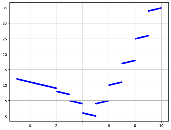
(b)

Fig. 1: (a) A weak-distance for check_sum, and (b) its visualization

This weak-distance approach avoids direct reasoning about floating-point semantics, allowing it to handle loops and external functions seamlessly. It has been successfully applied to satisfiability solving [15], automated testing [16], and boundary value analysis [17], often achieving an order-of-magnitude performance improvement over existing techniques.

1.0.2 Augmented Weak-Distance

Despite its advantages, weak distance suffers from two key limitations: (1) its constraints of non-negativity and zero-target correspondence are too weak, leading to flat landscapes (vanishing gradients) or misleading objectives; (2) it struggles with discontinuities from branching, which hinder optimization.

We address these issues with augmented weak-distance, contributing both theoretically and practically. Theoretically, we introduce an additional constraint, MCC, formalized via path-input affinity, which quantifies input closeness to an execution path by considering: (i) execution depth, tracking how far execution follows the expected path, and (ii) branch satisfaction, measuring how well branch conditions align with expected behavior. Embedding path-input affinity ensures a structured optimization landscape, overcoming flat or discontinuous regions. Practically, we develop a systematic algorithm for constructing augmented weak-distance functions. This algorithm dynamically traces execution paths and computes path affinity at runtime with minimal overhead, ensuring efficient floating-point analysis. As an alternative to symbolic execution, it avoids SMT solving and loop unwinding, enabling robust floating-point verification even in the presence of loops and external calls.

1.0.3 Empirical Results

We evaluated our method on the SV-COMP 2024 benchmark suite [3]. Across 40 benchmarks with known ground truths:

• Our approach achieved 100% accuracy, matching the state-of-the-art bounded model checker CBMC [20].

• Our method was 170 times faster than CBMC.

• The static analysis tool Astrée [10] was faster but solved only 17.5% of the benchmarks.

2 Weak Distance: Pitfalls and How We Address Them

As introduced in Sect. 1, the weak-distance approach embeds a global variable w = ... before each branch, capturing deviations from satisfying the branch condition. The weak distance function satisfies non-negativity and zero-target correspondence, theoretically ensuring that minimizing d leads to a solution.

However, theoretical correctness does not guarantee practical feasibility. Weak distance may mislead optimization due to abrupt changes in the landscape or discontinuities in execution paths, leading to premature convergence or missing valid solutions. We identify two key pitfalls: (1) Non-Monotonic Descent Disrupts Optimization—Abrupt jumps in the landscape mislead the optimizer, causing premature convergence. (2) Ignoring Per-Path Behavior Causes Incorrect Solutions—Weak distance assumes a globally smooth landscape, but execution paths may behave discontinuously.

The following sections illustrate these pitfalls and outline key principles for addressing them.

2.1 Example 1: Non-Monotonic Descent Disrupts Optimization

Consider the following example:

⬇

1void check_date(int day, int month) {

2 if (day == 20) {

3 if (month == 10)

4 printf("reached");

5 }

6}

List. 2: Sample function with nested if statements.

2.1.1 How Weak Distance is Normally Applied

To construct a weak-distance function, we introduce w as a global variable to capture how far the input deviates from satisfying key branch conditions. At each conditional check, w encodes the squared difference between the input variable and the expected value. This ensures non-negativity and zero-target correspondence but does not guarantee an informative gradient for optimization. Fig. 2 illustrates this weak distance construction.

⬇

1double WD(double d, double m){

2 int day = floor(d);

3 int month = floor(m);

4 d = (day - 20) ** 2;

5 if (day == 20){

6 d = (month - 10) ** 2;

7 if (month == 10)

8 printf("reached");

9}

⬇

1double AWD(double d, double m){

2 int day = floor(d);

3 int month = floor(m);

4 d = (day - 20) ** 2 + 150;

5 if (day == 20){

6 d = (month - 10) ** 2;

7 if (month == 10)

8 printf("reached");

9}

Fig. 2: C Weak-Distance (L) and Augmented Weak-Distance (R) for check_sum.

2.1.2 Why Weak Distance Fails

Although $\mathtt{WD}$ satisfies non-negativity and zero-target correspondence, it fails to guide optimization toward the correct target $(20,10)$. The failure can be observed in how the minimization process unfolds: (1) The optimizer minimizes $d$, reducing the squared distance from a starting point $(1,1)$. (2) It successfully moves along the $x$-axis, reaching $(19,1)$ where $d=1$. (3) However, when $x=20$, $d$ jumps to 81, increasing sharply. (4) The optimizer misinterprets this jump as an incorrect direction, causing it to halt prematurely at $(19,1)$.

Thus, the weak distance fails because closeness does not consistently correspond to a lower objective function value. A strictly decreasing objective function as the input approaches the solution is needed.

2.1.3 Fixing the Issue: Monotonic Convergence Condition (MCC)

To resolve this, we introduce the Monotonic Convergence Condition (MCC), ensuring a strictly decreasing objective function as the input approaches the solution:

MCC: The objective function must decrease monotonically as the solution is approached.

MCC accounts for two key aspects of closeness: (1) Execution depth—the objective should decrease as the realized execution path nears the target in the syntax tree, and (2) Branch satisfaction—the distance between the left- and right-hand sides of a branch, as already considered in weak distance. We formalize this in Sect. 3 as path-input affinity.

Fig. 2 modifies $\mathtt{WD}$ to construct an Augmented Weak-Distance function $\mathtt{AWD}$ by introducing a large offset (e.g., 150) before the first branch:

$$\text{d}=(\text{day}-20)^{2}+150.$$ (2)

This adjustment ensures that before satisfying the first branch ($\text{day}=20$), the function remains guided by $(\text{day}-20)^{2}$, while the added 150 has no effect. Once the first branch is met, the function transitions to the second branch, where it is now governed by $(\text{month}-10)^{2}$, a strictly smaller value than 150. This naturally guides the optimization deeper into the program, leading to $(\text{day}=20,\text{month}=10)$.

Fig. 3 illustrates how $\mathtt{AWD}$ corrects $\mathtt{WD}$’s misleading behavior by reshaping the optimization landscape. Unlike $\mathtt{WD}$, which introduces structural discontinuities that hinder convergence, $\mathtt{AWD}$ ensures a smoother descent, enabling the optimizer to reach the desired solution efficiently.

Have a few

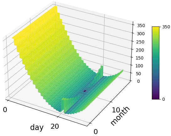
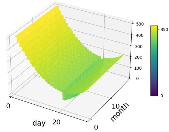
Fig. 3: Weak distance (L) and Augmented Weak Distance (R) for check_sum.

2.2 Example 2: Ignoring Per-Path Behavior Misses Solutions

Numerical programs often use the safe_reciprocal function:

$$\text{safe\_reciprocal}(x)=\begin{cases}1/x,&x\neq 0\\ 0,&x=0\end{cases}$$

to prevent division-by-zero, avoiding numerical instability and NaN propagation [2]. Consider the following program, which computes the cotangent of $x$ using safe_reciprocal, and checks whether the result is zero:

⬇

1double cot(double x) {

2 double y = safe_reciprocal(tan(x));

3 if (y == 0) printf("reach 0");

4 return y; }

List. 3: Program using safe_reciprocal to compute $\cot(x)$.

2.2.1 How Weak Distance is Normally Applied

The weak-distance method attempts to locate inputs that trigger "reach 0". A standard weak-distance function embeds d = (y - 0) ** 2; before the conditional statement, creating a function that maps the input $x$ to the global variable d.

⬇

1double WD(double x) {

2 double y = safe_reciprocal(tan(x));

3 d = (y - 0) ** 2; // Weak distance metric

4 if (y == 0) printf("reach 0");

5 return y;}

2.2.2 Why Weak Distance Fails

The weak-distance function creates a misleading optimization landscape, steering the optimizer away from $x=0$. The failure arises because weak distance lacks smoothness across its input range. Specifically, as $x$ approaches $\pi/2$, $y$ approaches 0, and the weak-distance function provides a smooth gradient, guiding the optimizer toward this solution. However, at $x=0$, weak distance increases, incorrectly signaling the optimizer to move away, despite it being a valid solution.

2.2.3 Fixing the Issue: Per-Path Optimization

To overcome this limitation, we introduce a per-path optimization approach, where each execution path is treated independently to avoid misleading discontinuities. Specifically, we separate execution paths: one solving for $x=0$, where $\tan(x)=0$, and another solving for $x=\pi/2$, where $\tan(x)\to\infty$. By treating each path separately, we restore smoothness within each optimization step, ensuring that numerical minimization correctly identifies all solutions. A potential downside of this approach is the need for explicit path enumeration. However, weak distance remains advantageous in handling loops and external function calls, as it naturally constructs numerical objectives that generalize across execution paths.

2.2.4 Takeaways

These examples highlight a fundamental limitation of weak distance: its properties of non-negativity and zero-target correspondence alone are insufficient when structural or numerical discontinuities exist in the optimization landscape. Weak distance fails because it treats all branches equally, ignoring both execution depth and path-dependent behavior. To overcome this, optimization must align with program structure and explicitly account for execution paths. The Monotonic Convergence Condition (MCC) ensures a strictly decreasing objective function, preventing misleading optima, while the per-path optimization strategy restores continuity and eliminates weak-distance misguidance. Together, these enhancements enable robust and accurate program analysis, even in the presence of branching, loops, and floating-point instability.

3 Foundations of Augmented Weak Distance

3.0.1 General Notation

We denote the set of non-negative integers by $\mathbb{Z}_{\geq 0}$, representing all integers greater than or equal to zero. The set of finite floating-point numbers in IEEE 754 (excluding NaN and infinity) [1] is denoted by $\mathbb{F}$. Given a function $f$, its input domain is written as $\mathit{dom}(f)$. The Cartesian product of two sets $A$ and $B$ is denoted as $A\times B$. The notation $\lambda x.f(x)$ defines an anonymous function, representing a function that takes an input $x$ and returns $f(x)$.

We use $\mathit{Prog}$ to denote a program, $\mathit{Br}$ for a branch, $\pi$ for a path, and $x$ for an input. A path is a sequence of branches, where each branch consists of a label and a Boolean outcome (true or false). . A path is partial if it forms a prefix of a complete execution path. Each input $x$ is treated as an $n$-dimensional floating-point vector, meaning that $\mathit{dom}(\mathit{Prog})\subseteq\mathbb{F}^{n}$ for some integer $n$.

The notation $\mathit{Prog}(x)$ represents the execution path taken by $\mathit{Prog}$ when executed with input $x$, which is a sequence of encountered branches.

Definition 1 (Bounds Checking)

Bounds checking is a reachability problem that determines whether a numerical bound, specified by an arithmetic comparison ($<,\leq,>,\geq,=$) between floating-point numbers, can be reached. Given a target program $\mathit{Prog}$ and a branch $\mathit{Br}$, the goal is to find an input $x$ such that the execution path $\mathit{Prog}(x)$ passes through $\mathit{Br}$.

3.1 Overall Solution

We solve the bounds checking problem using a per-path scheme to maximize precision. Specifically, for each execution path $\pi$ passing through $\mathit{Br}$, we seek an input that triggers $\pi$. The per-path strategy mitigates the risk of missing solutions (Sect. 2.2), but a key challenge arises in handling loops. However, as illustrated in List. 1, weak distance mitigates this issue by disregarding loops. Therefore, we start our solution with the following path synthesis step.

Let $\mathit{Paths}$ denote the set of synthesized paths from Step 1. To systematically evaluate each path, we construct an augmented weak distance function $\mathtt{AWD}$, extending weak distance to a per-path formulation:

$$\mathtt{AWD}:\mathit{Paths}\times\mathit{dom}(\mathit{Prog})\to\mathbb{F}.$$

The function $\mathtt{AWD}(\pi,x)$ takes a path $\pi\in\mathit{Paths}$ and an input $x\in\mathit{dom}(\mathit{Prog})$, returning a floating-point value that quantifies how close $x$ is to triggering $\pi$. We impose the following conditions to ensure its correctness:

• Non-negativity: For all $\pi\in\mathit{Paths}$ and $x\in\mathit{dom}(\mathit{Prog})$, $\mathtt{AWD}(\pi,x)\geq 0$.

• Zero-target correspondence: $\mathtt{AWD}(\pi,x)=0$ if and only if $x$ triggers $\pi$.

To address non-monotonic descent (Sect. 2.1), we impose:

• MCC: For each path $\pi\in\mathit{Paths}$, the function $\lambda x.\mathtt{AWD}(\pi,x)$ must decrease as $x$ moves closer to the target branch.

We will formalize "closeness" in the next section. Below is Step 2.

Once the $\mathtt{AWD}$ function is constructed, we proceed to minimize it to solve the bounds checking problem. Non-negativity and zero-target correspondence ensure that if $\min_{x}\mathtt{AWD}(\pi,x)=0$ for any $\pi$, then the corresponding minimizer ($\arg\min_{x}\mathtt{AWD}(\pi,x)$) represents an input that triggers $\pi$. The MCC condition guarantees that this optimization process is feasible. Thus, we conclude with:

3.2 Path-Input Affinity: Formalizing MCC

Let $\pi$ be a partial execution path terminating at $\mathit{Br}$, and let $\mathit{Prog}\{x\}$ denote the path taken by executing $\mathit{Prog}$ with input $x$. To formally define the notion of closeness between $\pi$ and $x$ required for the Monotonic Convergence Condition (MCC), we introduce a metric called path-input affinity. As motivated in Sect. 2.1, this metric captures two key aspects: (1) how deeply the realized path aligns with the expected path, and (2) how close the branch condition at the fork (where $\mathit{Prog}\{x\}$ and $\pi$ diverge) is to being satisfied.

3.2.1 Preliminary Definitions

We first introduce the necessary building blocks to define path-input affinity rigorously.

The Floating-Point Cardinality between two floating-point numbers $a,b\in\mathbb{F}$ is defined as the number of distinct floating-point values $x\in\mathbb{F}$ such that $\min(a,b)\leq x<\max(a,b)$. We denote this count by $\kappa(a,b)$. Clearly, $0\leq\kappa(a,b)\leq 2^{64}$ for double-precision floating-point numbers.

We define the lexicographic order $\prec$ over $\mathbb{Z}_{\geq 0}\times\mathbb{Z}_{\geq 0}$ as:

$$(x^{\prime},y^{\prime})\prec(x,y)\quad\iff\quad x^{\prime}<x\quad\text{or}\quad(x^{\prime}=x\text{ and }y^{\prime}<y).$$

For example, $(3,27)\prec(10,1)$ and $(3,27)\prec(3,42)$.

The fork branch, or simply fork, between two paths is the first branch where they diverge. If one path subsumes the other, the fork does not exist.

Definition 2 (Path-Input Affinity)

Given a bounds checking problem $(\mathit{Prog},\mathit{Br})$, let $\mathit{Paths}$ denote the set of partial paths ending at $\mathit{Br}$. The path-input affinity quantifies the closeness between a path $\pi$ and an input $x$ as:

$$\mathit{Aff}:\mathit{Paths}\times\text{dom}(\mathit{Prog})\to\mathbb{Z}_{\geq 0}^{2},$$

where $\mathit{Aff}(\pi,x)=(u,v)$ is defined as follows: $u$ is the number of branches in $\pi$ starting from the fork branch; if the fork does not exist, $u=0$; $v$ is the number of floating-point values between the left-hand side (lhs) and right-hand side (rhs) of the fork branch; if no fork exists, $v=0$.

The precise computation of $v$ is given by:

$$v=\begin{cases}\kappa(\text{lhs},\text{rhs})&\text{if the fork branch is }\text{lhs}\leq\text{rhs},\text{lhs}\geq\text{rhs},\text{or }\text{lhs}=\text{rhs},\\ \kappa(\text{lhs},\text{rhs})+1&\text{if the fork branch is }\text{lhs}<\text{rhs},\text{lhs}>\text{rhs},\\ 1&\text{if the fork branch is }\text{lhs}\neq\text{rhs}.\end{cases}$$

3.2.2 Example

Consider the following program:

⬇

1void foo(double x) {

2 if (x <= 3.0) error();

3}

Let the target path be $\pi=[0T]$, where $0$ denotes the label for the if condition. Then:

$$\mathit{Aff}(\pi,3.2)=(1,\kappa(3.2,3))\quad\text{and}\quad\mathit{Aff}(\pi,2.9)=(0,0).$$

3.2.3 Formalizing MCC with Path-Input Affinity

With the notion of path-input affinity established, we can now express the MCC condition formally. For any $\pi\in\mathit{Paths}$ and any two inputs $x,x^{\prime}\in\mathit{dom}(\mathit{Prog})$,

$$\mathit{Aff}(\pi,x^{\prime})\prec\mathit{Aff}(\pi,x)\quad\Rightarrow\quad\mathtt{AWD}(\pi,x^{\prime})<\mathtt{AWD}(\pi,x).$$

This guarantees that as an input $x$ becomes closer to triggering $\pi$ (in the sense of affinity), the corresponding $\mathtt{AWD}$ value strictly decreases, ensuring convergence in the optimization process.

3.3 AWD Function and its Mathematical Properties

We define the $\mathtt{AWD}$ function as any implementation satisfying the interface $\mathit{Paths}\times\mathit{dom}(\mathit{Prog})\to\mathbb{F}$ that adheres to the following three properties: non-negativity, zero-target correspondence, and the Monotonic Convergence Condition (MCC). The MCC ensures that for a fixed $\pi$, if $\mathit{Aff}(\pi,x)$ decreases, then $\mathtt{AWD}(\pi,x)$ must also decrease. Since $\mathtt{AWD}$ returns a scalar value, ensuring compliance with MCC requires an encoding that preserves the lexicographic order $\prec$.

To achieve this, we construct $\mathtt{AWD}$ as follows:

$$\mathtt{AWD}(\pi,x)=u\cdot M+v,\quad\text{where }(u,v)=\mathit{Aff}(\pi,x).$$ (3)

Here, $M$ is chosen such that $M>\max(v)$ for all possible values of $v$, ensuring correct order preservation. Fig. 4 illustrates the fork branch concept and the definition of $\mathtt{AWD}$.

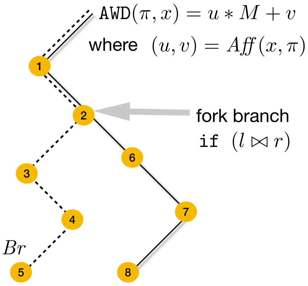
Fig. 4: The fork branch and the $\mathtt{AWD}$ function.

The function defined in Eq. (3) satisfies non-negativity and zero-target correspondence since $u$, $v$, and $M$ are non-negative by construction. The crucial property that establishes MCC follows from the lemma below, which ensures that the encoding $E(u,v)$ correctly preserves the lexicographic order:

Lemma 1

Let $(u_{1},v_{1})$ and $(u_{2},v_{2})$ be two pairs ordered lexicographically. Define the mapping $E(u,v)=uM+v$, where $M>\max(v)$ for all possible $v$. Then $E(u,v)$ preserves the lexicographic order:

1. If $u_{1}<u_{2}$, then $E(u_{1},v_{1})<E(u_{2},v_{2})$.

2. If $u_{1}=u_{2}$ and $v_{1}<v_{2}$, then $E(u_{1},v_{1})<E(u_{2},v_{2})$.

Proof (Proof Sketch)

We show that the mapping $E(u,v)=uM+v$, where $M>\max(v)$, preserves lexicographic order. If $u_{1}<u_{2}$, then $u_{1}M<u_{2}M$, and since $v_{1},v_{2}\geq 0$, adding them does not reverse the inequality, ensuring $E(u_{1},v_{1})<E(u_{2},v_{2})$. If $u_{1}=u_{2}$ and $v_{1}<v_{2}$, then $E(u_{1},v_{1})=u_{1}M+v_{1}$ and $E(u_{2},v_{2})=u_{2}M+v_{2}$, reducing to $v_{1}<v_{2}$, so $E(u_{1},v_{1})<E(u_{2},v_{2})$. The condition $M>\max(v)$ is necessary; otherwise, a large enough $v_{1}$ could dominate the difference $(u_{2}-u_{1})M$, violating order preservation.

3.4 Algorithmic Construction of the AWD Function

To construct the $\mathtt{AWD}$ function, we need to compute Eq. 3. The process of constructing $\mathtt{AWD}$ follows these steps: (1) We introduce three global variables: paths, beats, and d. The variable paths serves as one of the two inputs to $\mathtt{AWD}$, preserving the interface $\mathit{Paths}\times\mathit{dom}(\mathit{Prog})\to\mathbb{F}$ without altering the original interface of $\mathit{Prog}$. Similarly, d represents the output of $\mathtt{AWD}$, ensuring the original output type of $\mathit{Prog}$ remains intact. The variable beats tracks the execution progress along the expected path, which we use for identifying the fork branch and computing $u$ in Eq. 3. (2) Given an input $x\in\mathit{dom}(\mathit{Prog})$, we require that $\mathtt{AWD}(\pi,x)$ returns zero if $x$ follows the expected path $\pi$; otherwise, it identifies the fork branch, computes $(u,v)=\mathit{Aff}(\pi,x)$, and updates d following Eq. 3.

To implement this, we embed a branch sentinel within the program under analysis to identify fork branches and compute $(u,v)$ in the path affinity function. The branch sentinel is a callback function that dynamically updates d based on three execution stages: (1) if the realized path matches $\pi$ completely, then $\texttt{d}=0$; (2) if it partially matches, d accumulates a distance proportional to the unmatched branches; (3) if it diverges at a fork, d incorporates the operand distance $v$, scaled by the remaining unmatched depth. Algorithm 1 illustrates the design of the branch sentinel. Embedding the sentinel as a callback function before each branch ensures that the constructed $\mathtt{AWD}$ function correctly computes Eq. 3 and satisfies the required conditions of non-negativity, zero-target correspondence, and monotonic convergence.

As an implementation detail, we use $\texttt{v}=\ln(1+\texttt{v\_original}))$ instead of v_original itself as one might expect from Def. 2. This modification maintains the correctness of the algorithm due to Lem. 1 and ensures that value of M that is larger than any v, can be found.

1

2

Input: cond: Branch condition
op: Comparison operator
lhs, rhs: Operands for comparison

Output: d

;

 // paths, beats, d are global variables. M is a large number.

3 if disable_sen is true then

4    return

5expected_br $\leftarrow$ paths[beats] ;

6 realized_br $\leftarrow$ Compare(op, lhs, rhs) ;

7

8beats $\leftarrow$ beats + 1 ;

9

10if expected_br = realized_br and beats = paths.length then

    d $\leftarrow 0$ ;

    // Entire path matched

11    disable_sen $\leftarrow$ true ;

12   

13else if expected_br = realized_br then

    d $\leftarrow-42$ ;

    // Partial progress, placeholder value to be overwritten

14   

15else

    ;

    // Fork branch

16    $\texttt{u}\leftarrow\texttt{paths.length}-\texttt{beats}$ ;

17    $\texttt{v\_original}\leftarrow\kappa(\texttt{lhs},\texttt{rhs},\kappa(\texttt{lhs},\texttt{rhs}+1,\text{ or 1 depending on }\texttt{op}$ (Def. 2) ;

18    $\texttt{v}\leftarrow\ln(1+\texttt{v\_original})$ ;

19    $\texttt{d}\leftarrow\texttt{u * M + v}$ ;

20    disable_sen $\leftarrow$ true ;

21   

Algorithm 1 Embedded Branch Sentinel: sen

4 Experiments

5 Implementation

We implement AWD as a research prototype in Python and C++. The input is a tuple $(M,F,T)$, where $M$ is an LLVM IR module, $F$ is the entry function, and $T$ is the target identifier (e.g., __error). The output is a reachability verdict, optionally providing a triggering input.

Our implementation consists of three main components. (1) The LLVM pass paths.cc synthesizes execution paths to $T$ using breadth-first search over the control flow graph, tracking partial paths under depth and call stack constraints. Handling loops and external calls as branches remains a future extension. (2) The embed.cc pass instruments conditional branches by inserting type-aware function calls via llvm::IRBuilder, ensuring program semantics remain intact while enabling precise tracking. (3) Global optimization, implemented in min.py, minimizes $\mathtt{AWD}(\pi,x)$ for each synthesized path, seeking inputs that reach zero. We use basinhopping, a stochastic optimizer leveraging random perturbations and MCMC acceptance criteria, with Powell for local refinement. The AWD function is dynamically loaded as euler.so and invoked via Python’s ctypes, avoiding inter-process overhead. To ensure correctness, we enforce nonnegativity constraints and classify reachability based on the computed minima.

5.1 Experimental Setup

We evaluated AWD on all 40 benchmarks from SV-COMP 2024’s floats-cdfpl category [3, 4], designed for bounds checking [12]. Each C benchmark has a known ground truth (G.T in Tab. 1) as either reachable (REA) or unreachable (UNR).

We compared AWD against two verification tools: static analyzer Astrée [10] and C bounded model checker CBMC [20] which combines bounded model checking and symbolic execution. Astrée is a proprietary static analysis tool. Since it is not freely available, we did not run it but used recorded results from previous executions on the same set of benchmarks, as documented in [11]. CBMC is an actively developed tool widely recognized for software verification, particularly for its capability in floating-point verification.

Other potential comparison methods were considered but ultimately excluded. (1) Weak Distance Methods [17]: While initially considered, weak-distance-based approaches failed to handle even the simplest branching structures, as shown in Sect. 2. (2) Conflict-Driven Learning (CDL) [12]: Originally developed over a decade ago, CDL does not appear to be actively maintained. Additionally, its original authors are now among the primary developers of CBMC. Given CBMC’s status as a leading floating-point verification tool, we consider it the more relevant and representative comparison.

All AWD and CBMC experiments were conducted on a MacBook Air equipped with an Apple M3 chip and 24GB of memory, running macOS Sequoia 15.1. As mentioned above, recorded results from [11] were used for Astrée.

5.2 Accuracy Comparison

As shown in Table 1, AWD achieved 100% accuracy, correctly classifying all benchmarks as either reachable (REA) or unreachable (UNR). In contrast, Astrée solved only 17.5% of the cases, demonstrating its limitations in handling floating-point constraints, while CBMC also achieved 100% accuracy. These results confirm that AWD provides the same level of precision as model checking while significantly outperforming static analysis.

A sanity check was performed, as shown in columns 3 and 4 of the table. Whenever the AWD function reached a minimum value of $0$, AWD consistently returned REA, correctly matching the ground truth classification of REA (reachable). This outcome aligns with theoretical expectations and further reinforces the reliability of AWD’s optimization-based approach.

The comparison against Astrée may appear problematic. As a static analysis tool based on over-approximation through abstract interpretation [9], Astrée’s primary strength lies in proving that erroneous behaviors will never occur in any execution of the analyzed program. In other words, Astrée is designed to establish unreachability (absence of bugs) rather than verify reachability (presence of bugs), although it can be used for the latter with a tight abstraction [26]. This limitation is evident in the results, as Astrée failed in all cases requiring reachability verification. However, if we consider only the 23 benchmarks where the ground truth is unreachability (UNR), a more appropriate evaluation of Astrée’s accuracy emerges. In this case, Astrée correctly identified 7 out of 23, resulting in an adjusted accuracy of 30.4%, which may be insufficient for practical bounds checking compared to AWD.

Tab. 1: Benchmark Results: Accuracy and Execution Time of AWD, CBMC, and Astrée for Floating-Point Bounds Checking. G. T. refers to the ground truth classification, where UNR indicates an unreachable state and REA indicates a reachable state.

Benchmark		AWD Results		Accuracy			Time (seconds)
Name	G. T.	Minimum	Verict	ASTREE	CBMC	AWD	ASTREE	CBMC	AWD
newton_1_1	UNR	1.97E-01	UNR	✓	✓	✓	0.05	8.08	0.55
newton_1_2	UNR	1.77E-01	UNR	✓	✓	✓	0.05	38.25	0.53
newton_1_3	UNR	1.16E-01	UNR	—	✓	✓	0.05	62.73	0.53
newton_1_4	REA	0	REA	—	✓	✓	0.05	2.75	0.52
newton_1_5	REA	0	REA	—	✓	✓	0.05	1.28	0.52
newton_1_6	REA	0	REA	—	✓	✓	0.05	3.97	0.54
newton_1_7	REA	0	REA	—	✓	✓	0.04	3.62	0.53
newton_1_8	REA	0	REA	—	✓	✓	0.05	3.40	0.55
newton_2_1	UNR	2.00E-01	UNR	✓	✓	✓	0.06	132.97	0.52
newton_2_2	UNR	2.00E-01	UNR	✓	✓	✓	0.06	80.84	0.55
newton_2_3	UNR	2.00E-01	UNR	—	✓	✓	0.06	78.30	0.54
newton_2_4	UNR	1.96E-01	UNR	—	✓	✓	0.06	77.34	0.54
newton_2_5	UNR	1.37E-01	UNR	—	✓	✓	0.06	132.82	0.56
newton_2_6	REA	0	REA	—	✓	✓	0.06	61.42	0.54
newton_2_7	REA	0	REA	—	✓	✓	0.05	205.25	0.54
newton_2_8	REA	0	REA	—	✓	✓	0.04	11.47	0.57
newton_3_1	UNR	2.00E-01	UNR	✓	✓	✓	0.06	182.19	0.53
newton_3_2	UNR	2.00E-01	UNR	✓	✓	✓	0.06	226.46	0.56
newton_3_3	UNR	2.00E-01	UNR	✓	✓	✓	0.06	842.97	0.56
newton_3_4	UNR	2.00E-01	UNR	—	✓	✓	0.06	223.78	0.55
newton_3_5	UNR	2.00E-01	UNR	—	✓	✓	0.06	228.78	0.55
newton_3_6	REA	0	REA	—	✓	✓	0.06	105.55	0.56
newton_3_7	REA	0	REA	—	✓	✓	0.05	67.35	0.54
newton_3_8	REA	0	REA	—	✓	✓	0.06	55.55	0.56
sine_1	REA	0	REA	—	✓	✓	0.02	0.40	0.56
sine_2	REA	0	REA	—	✓	✓	0.02	1.38	0.53
sine_3	REA	0	REA	—	✓	✓	0.02	1.16	0.59
sine_4	UNR	1.01E-01	UNR	—	✓	✓	0.02	663.80	0.54
sine_5	UNR	1.91E-01	UNR	—	✓	✓	0.02	15.22	0.53
sine_6	UNR	2.91E-01	UNR	—	✓	✓	0.02	15.76	0.56
sine_7	UNR	5.91E-01	UNR	—	✓	✓	0.02	7.22	0.55
sine_8	UNR	1.09E+00	UNR	—	✓	✓	0.02	16.96	0.54
square_1	REA	0	REA	—	✓	✓	0.01	1.11	0.56
square_2	REA	0	REA	—	✓	✓	0.02	0.86	0.56
square_3	REA	0	REA	—	✓	✓	0.02	0.70	0.55
square_4	UNR	1.00E-01	UNR	—	✓	✓	0.02	61.41	0.55
square_5	UNR	1.00E-01	UNR	—	✓	✓	0.02	52.32	0.55
square_6	UNR	1.01E-01	UNR	—	✓	✓	0.02	52.81	0.55
square_7	UNR	1.02E-01	UNR	—	✓	✓	0.02	36.01	0.57
square_8	UNR	2.02E-01	UNR	—	✓	✓	0.02	0.42	0.56
SUMMARY				17.50%	100%	100%	0.04	94.12	0.55

5.3 Execution Time Comparison

AWD demonstrates a substantial performance advantage over CBMC, significantly reducing execution time across all benchmarks. On average, AWD completed each benchmark in 0.55 seconds, whereas CBMC required 94.12 seconds per benchmark. This corresponds to a 170X speedup, highlighting AWD’s efficiency in solving bounds-checking problems.

Astrée was fastest at 0.04s but lacked accuracy, making it unreliable. AWD balances speed and accuracy, providing a practical bounds-checking solution.

CBMC is particularly slow on certain Newton benchmarks; it took 205.25 seconds on newton_2_7, while AWD solved it in 0.54 seconds. The most extreme case, newton_3_3, required 842.97 seconds for CBMC but only 0.56 seconds for AWD. In contrast, AWD maintains a nearly constant execution time of approximately 0.55 seconds across all benchmarks. This stability likely stems from its execution-based approach, where runtime depends on program execution rather than reasoning overhead. Since all benchmarks are small but vary in complexity, AWD avoids the drastic slowdowns seen in CBMC.

6 Discussion

Theoretical Boundaries and Guarantees

The augmented weak-distance (AWD) approach extends weak distance but also inherits its theoretical limitations. In general, global optimization may fail to return a true global minimum. To formalize this limitation, we use the notation $\hat{x}^{*}$ to denote the global minimum point found by a mathematical optimization backend for a given path $\pi$, and $x^{*}$ to denote the true global minimum. Then, we have:

$$\mathtt{AWD}(\pi,\hat{x}^{*})\geq\mathtt{AWD}(\pi,x^{*}).$$

Consider two cases. If $\mathtt{AWD}(\pi,\hat{x}^{*})=\mathtt{AWD}(\pi,x^{*})$, meaning the optimization backend finds the correct minimum, then the zero-target correspondence property ensures that AWD produces the correct verdict, whether the path is reachable or unreachable. However, if $\mathtt{AWD}(\pi,\hat{x}^{*})>\mathtt{AWD}(\pi,x^{*})$ and additionally $\mathtt{AWD}(\pi,\allowbreak x^{*})=0$, then AWD will incorrectly report the path as unreachable, failing to detect a valid bound. Depending on how reachability is framed, this issue may be classified as incompleteness or unsoundness.

Loops and External Calls: Design Trade-offs and Challenges

While AWD mitigates path explosion by ignoring branches within loops and treating external functions as opaque constructs, this simplification risks overlooking target branches that reside within a loop or an external function. For instance, in the check_sum example (Sect. 1), if the condition sum + decimal == 11 were placed inside the loop spanning lines 6 to 97, our current solution would fail to trigger it. This limitation becomes particularly problematic when critical conditions are nested within loops or hidden inside external functions, as these branches are effectively excluded from the path exploration process.

Beyond Floating-Point

Inputs that are not floating-point numbers must be transformed into floating-point representations to leverage the optimization process. This transformation is straightforward for primary data types such as integers or unsigned numbers. However, handling complex types, such as pointers or custom data structures, requires specialized mappings that preserve semantic meaning. Automating this process is non-trivial and inherently limited.

When dealing with conditional branches based on non-floating-point properties, such as if Prop(a), where Prop(a) evaluates to true or false, the current implementation can only assign a binary distance, which provides no gradient information to guide the optimization process. Otherwise, if Prop(a) is a simple function, it can be inlined or incorporated directly into the path synthesis process during the path synthesis. For example, this strategy works well for handling branches in the safe_reciprocal function (Sect. 2). However, when Property(a) involves inaccessible library functions or contains a large number of branches, this approach becomes infeasible.

7 Related Work

This section reviews related work and positions our contributions. Our approach builds upon the weak distance framework [17], which transforms program analysis problems into mathematical optimization tasks by minimizing an objective function. This paradigm has been extensively explored in the programming languages domain, with applications such as stochastic validation of compilers [25], search-based testing [18], floating-point satisfiability solving [15], and coverage-based testing [16]. A fundamental distinction between weak distance and traditional heuristic-based search methods lies in theoretical guarantees. While heuristic approaches (e.g., search-based testing) aim to minimize a cost function, they often lack assurances that the computed minima correspond to the intended program behavior [23]. In contrast, weak distance guarantees that the global minimum corresponds to a valid input triggering the target program behavior. Our work extends this guarantee by introducing a theoretical condition that ensures efficient convergence, thereby improving robustness and usability.

Bounds checking, also known as numerical bound analysis [12], represents an ideal application domain for AWD due to its emphasis on numerical computations. Unlike symbolic execution [5], which encodes floating-point operations using bit-vector logic such as QF_BVFP [7] and relies on NP-complete decision procedures [21], AWD turns the challenge of floating-point analysis into an opportunity of leveraging numerical techniques for improved efficiency. While symbolic execution is effective for verifying complex programs involving heap structures [24], its generality often leads to scalability challenges, as demonstrated in recent empirical studies [28]. By focusing on numerical computations, AWD achieves significantly improved performance in bounds checking.

Traditional tools for verifying numerical properties include static analyzers such as Astrée [10], model checkers like CBMC [20], symbolic execution engines such as KLEE [8], and SAT/SMT-based approaches like Conflict-Driven Learning (CDL) [12]. Each of these techniques has distinct strengths and limitations. CDL appears to be no longer actively maintained, and weak-distance-based approaches, despite their theoretical appeal, struggle with even simple branching structures, making them impractical for bounds checking. CBMC, as a bounded model checker with a symbolic execution backend, remains one of the most successful tools in floating-point verification and is widely used in verification competitions. Consequently, our evaluation focuses on Astrée and the latest available version of CBMC, as they represent state-of-the-art tools in static analysis, model checking, and symbolic execution for floating-point verification.

More broadly, Mathematical Optimization [6, 8] is a fundamental tool in computer science. It serves as the backbone of modern machine learning, enabling the optimization of objective functions for specific domains, such as loss functions in deep learning [22] and policy functions in reinforcement learning [27]. Similarly, weak distance and augmented weak distance focus on designing effective objective functions, but within the context of program analysis. Our work identifies fundamental issues in the weak distance objective function and proposes augmented weak distance to overcome these limitations, ensuring more reliable and efficient optimization in floating-point program verification.

8 Conclusion

In this paper, we introduced an augmented weak-distance framework, extending the theoretical foundations of weak-distance optimization to address its key limitations in numerical bounds verification. By overcoming branching discontinuity through a per-path approach, and overcoming insufficient theoretical conditions by introducing a new condition, Monotonic Convergence Condition (MCC), we ensure practical optimization landscapes that are both theoretically valid and computationally effective while maintaining the theoretical guarantees of the original weak-distance framework.

Our approach was rigorously validated on the SV-COMP 2024 benchmark suite that were used in bounds checking, achieving 100% accuracy across 40 benchmarks with known ground truths. This significantly outperformed existing techniques, including static analysis, model checking, and conflict-driven learning, both in accuracy and execution time, demonstrating the practical utility of the augmented framework.

The theoretical contributions of our work—particularly the formalization of path-input affinity and the design of the Euler function—lay the groundwork for future extensions. Moving forward, we aim to generalize this framework to handle non-numerical program constructs, such as heap-manipulating programs, while also scaling it to larger, more complex benchmarks.

References

- [1] Ieee standard for floating-point arithmetic. Standard IEEE Std 754-2008, IEEE Computer Society, New York, NY, USA (Aug 2008), https://web.archive.org/web/20160806053349/http://www.csee.umbc.edu/˜tsimo1/CMSC455/IEEE-754-2008.pdf
- [2] Bengio, Y.: Practical recommendations for gradient-based training of deep architectures. In: Neural networks: Tricks of the trade: Second edition, pp. 437–478. Springer (2012)
- [3] Beyer, D.: Sv-comp 2024: The 13th international competition on software verification (2024), https://sv-comp.sosy-lab.org/2024/, accessed: 2024-01-31
- [4] Beyer, D., et al.: Sv-benchmarks: Benchmark suite for software verification (2024), https://gitlab.com/sosy-lab/benchmarking/sv-benchmarks/-/tree/main/c/floats-cdfpl, accessed: 2024-01-31
- [5] de Boer, F.S., Bonsangue, M.M.: Symbolic execution formally explained. Formal Aspects Comput. 33(4-5), 617–636 (2021). https://doi.org/10.1007/S00165-020-00527-Y, https://doi.org/10.1007/s00165-020-00527-y
- [6] Boyd, S.P., Vandenberghe, L.: Convex Optimization. Cambridge University Press (2014). https://doi.org/10.1017/CBO9780511804441, https://web.stanford.edu/%7Eboyd/cvxbook/
- [7] Brain, M., Schanda, F., Sun, Y.: Building better bit-blasting for floating-point problems. In: Vojnar, T., Zhang, L. (eds.) Tools and Algorithms for the Construction and Analysis of Systems - 25th International Conference, TACAS 2019, Held as Part of the European Joint Conferences on Theory and Practice of Software, ETAPS 2019, Prague, Czech Republic, April 6-11, 2019, Proceedings, Part I. Lecture Notes in Computer Science, vol. 11427, pp. 79–98. Springer (2019). https://doi.org/10.1007/978-3-030-17462-0_5, https://doi.org/10.1007/978-3-030-17462-0_5
- [8] Cadar, C., Dunbar, D., Engler, D.R.: KLEE: unassisted and automatic generation of high-coverage tests for complex systems programs. In: Draves, R., van Renesse, R. (eds.) 8th USENIX Symposium on Operating Systems Design and Implementation, OSDI 2008, December 8-10, 2008, San Diego, California, USA, Proceedings. pp. 209–224. USENIX Association (2008), http://www.usenix.org/events/osdi08/tech/full_papers/cadar/cadar.pdf
- [9] Cousot, P., Cousot, R.: Systematic design of program analysis frameworks. In: Aho, A.V., Zilles, S.N., Rosen, B.K. (eds.) Conference Record of the Sixth Annual ACM Symposium on Principles of Programming Languages, San Antonio, Texas, USA, January 1979. pp. 269–282. ACM Press (1979). https://doi.org/10.1145/567752.567778, https://doi.org/10.1145/567752.567778
- [10] Cousot, P., Cousot, R., Feret, J., Mauborgne, L., Miné, A., Monniaux, D., Rival, X.: Combination of abstractions in the astrée static analyzer. In: Okada, M., Satoh, I. (eds.) Advances in Computer Science - ASIAN 2006. Secure Software and Related Issues, 11th Asian Computing Science Conference, Tokyo, Japan, December 6-8, 2006, Revised Selected Papers. Lecture Notes in Computer Science, vol. 4435, pp. 272–300. Springer (2006). https://doi.org/10.1007/978-3-540-77505-8_23, https://doi.org/10.1007/978-3-540-77505-8_23
- [11] Developers, C.: Cprover benchmark repository. https://www.cprover.org/cdfpl/ (2024), accessed: 2024-01-31
- [12] D’Silva, V.V., Haller, L., Kroening, D., Tautschnig, M.: Numeric bounds analysis with conflict-driven learning. In: Flanagan, C., König, B. (eds.) Tools and Algorithms for the Construction and Analysis of Systems - 18th International Conference, TACAS 2012, Held as Part of the European Joint Conferences on Theory and Practice of Software, ETAPS 2012, Tallinn, Estonia, March 24 - April 1, 2012. Proceedings. Lecture Notes in Computer Science, vol. 7214, pp. 48–63. Springer (2012). https://doi.org/10.1007/978-3-642-28756-5_5, https://doi.org/10.1007/978-3-642-28756-5_5
- [13] Euler, L.: Methodus inveniendi lineas curvas maximi minimive proprietate gaudentes sive solutio problematis isoperimetrici latissimo sensu accepti, vol. 1. Springer Science & Business Media (1952)
- [14] Fu, Z., Bai, Z., Su, Z.: Automated backward error analysis for numerical code. In: Aldrich, J., Eugster, P. (eds.) Proceedings of the 2015 ACM SIGPLAN International Conference on Object-Oriented Programming, Systems, Languages, and Applications, OOPSLA 2015, part of SPLASH 2015, Pittsburgh, PA, USA, October 25-30, 2015. pp. 639–654. ACM (2015). https://doi.org/10.1145/2814270.2814317, https://doi.org/10.1145/2814270.2814317
- [15] Fu, Z., Su, Z.: Xsat: A fast floating-point satisfiability solver. In: Chaudhuri, S., Farzan, A. (eds.) Computer Aided Verification - 28th International Conference, CAV 2016, Toronto, ON, Canada, July 17-23, 2016, Proceedings, Part II. Lecture Notes in Computer Science, vol. 9780, pp. 187–209. Springer (2016). https://doi.org/10.1007/978-3-319-41540-6_11, https://doi.org/10.1007/978-3-319-41540-6_11
- [16] Fu, Z., Su, Z.: Achieving high coverage for floating-point code via unconstrained programming. In: Cohen, A., Vechev, M.T. (eds.) Proceedings of the 38th ACM SIGPLAN Conference on Programming Language Design and Implementation, PLDI 2017, Barcelona, Spain, June 18-23, 2017. pp. 306–319. ACM (2017). https://doi.org/10.1145/3062341.3062383, https://doi.org/10.1145/3062341.3062383
- [17] Fu, Z., Su, Z.: Effective floating-point analysis via weak-distance minimization. In: McKinley, K.S., Fisher, K. (eds.) Proceedings of the 40th ACM SIGPLAN Conference on Programming Language Design and Implementation, PLDI 2019, Phoenix, AZ, USA, June 22-26, 2019. pp. 439–452. ACM (2019). https://doi.org/10.1145/3314221.3314632, https://doi.org/10.1145/3314221.3314632
- [18] Harman, M., McMinn, P.: A theoretical and empirical study of search-based testing: Local, global, and hybrid search. IEEE Trans. Software Eng. 36(2), 226–247 (2010). https://doi.org/10.1109/TSE.2009.71, https://doi.org/10.1109/TSE.2009.71
- [19] Iwamatsu, M., Okabe, Y.: Basin hopping with occasional jumping. Chemical Physics Letters 399(4-6), 396–400 (2004)
- [20] Kroening, D., Schrammel, P., Tautschnig, M.: CBMC: the C bounded model checker. CoRR abs/2302.02384 (2023). https://doi.org/10.48550/ARXIV.2302.02384, https://doi.org/10.48550/arXiv.2302.02384
- [21] Kroening, D., Strichman, O.: Decision Procedures - An Algorithmic Point of View, Second Edition. Texts in Theoretical Computer Science. An EATCS Series, Springer (2016). https://doi.org/10.1007/978-3-662-50497-0, https://doi.org/10.1007/978-3-662-50497-0
- [22] LeCun, Y., Bengio, Y., Hinton, G.: Deep learning. nature 521(7553), 436–444 (2015)
- [23] Perera, A., Turhan, B., Aleti, A., Böhme, M.: On the impact of lower recall and precision in defect prediction for guiding search-based software testing. ACM Trans. Softw. Eng. Methodol. 33(6), 144 (2024). https://doi.org/10.1145/3655022, https://doi.org/10.1145/3655022
- [24] Rajput, A., Gopinath, K.: GARUDA: heap aware symbolic execution. In: 44th IEEE/ACM International Conference on Software Engineering: Companion Proceedings, ICSE Companion 2022, Pittsburgh, PA, USA, May 22-24, 2022. pp. 352–353. ACM/IEEE (2022). https://doi.org/10.1145/3510454.3528650, https://doi.org/10.1145/3510454.3528650
- [25] Schkufza, E., Sharma, R., Aiken, A.: Stochastic superoptimization. In: Sarkar, V., Bodík, R. (eds.) Architectural Support for Programming Languages and Operating Systems, ASPLOS 2013, Houston, TX, USA, March 16-20, 2013. pp. 305–316. ACM (2013). https://doi.org/10.1145/2451116.2451150, https://doi.org/10.1145/2451116.2451150
- [26] Stein, B., Chang, B.E., Sridharan, M.: Demanded abstract interpretation. In: Freund, S.N., Yahav, E. (eds.) PLDI ’21: 42nd ACM SIGPLAN International Conference on Programming Language Design and Implementation, Virtual Event, Canada, June 20-25, 2021. pp. 282–295. ACM (2021). https://doi.org/10.1145/3453483.3454044, https://doi.org/10.1145/3453483.3454044
- [27] Wiering, M.A., Van Otterlo, M.: Reinforcement learning. Adaptation, learning, and optimization 12(3), 729 (2012)
- [28] Yang, X., Zhang, G., Shuai, Z., Chen, Z., Wang, J.: Symbolic execution of floating-point programs: How far are we? J. Syst. Softw. 220, 112242 (2025). https://doi.org/10.1016/J.JSS.2024.112242, https://doi.org/10.1016/j.jss.2024.112242