Safe Primal-Dual Optimization with a Single Smooth Constraint

Abstract

This paper addresses the problem of safe optimization under a single smooth constraint, a scenario that arises in diverse real-world applications such as robotics and autonomous navigation. The objective of safe optimization is to solve a black-box minimization problem while strictly adhering to a safety constraint throughout the learning process. Existing methods often suffer from high sample complexity due to their noise sensitivity or poor scalability with number of dimensions, limiting their applicability. We propose a novel primal-dual optimization method that, by carefully adjusting dual step-sizes and constraining primal updates, ensures the safety of both primal and dual sequences throughout the optimization. Our algorithm achieves a convergence rate that significantly surpasses current state-of-the-art techniques. Furthermore, to the best of our knowledge, it is the first primal-dual approach to guarantee safe updates. Simulations corroborate our theoretical findings, demonstrating the practical benefits of our method. We also show how the method can be extended to multiple constraints.

Keywords: safe leaning, black-box optimization, primal-dual method

1 Introduction

Motivation

The safe learning problem is becoming more relevant nowadays with growth of automatization, usage of reinforcement learning, and learning from interactions. In such problems, it is crucial not to violate safety constraints during the learning, even if they are not known in advance. As an example, imagine the task of real-time parameter tuning in manufacturing or control settings (Koenig et al., 2023; Dogru et al., 2022). The goal is to minimize production costs or maximize performance without compromising safety constraints during the real-time world interactions. Moreover, one might only have black-box, noisy measurements of safety and cost, and their estimated gradients, without access to their precise analytical expressions or models. Then, one aims to iteratively update the parameters and simultaneously take measurements, aiming to find parameters with better cost. It is crucial to ensure the constraints not being violated during the learning process. In many cases, the safety constraint is a single constraint, e.g., when safety must be ensured by limiting the probability of hitting the obstacles in robotics and reinforcement learning (Ray et al., 2019), by limiting the velocity error in automatic controller tuning (König et al., 2023), or ensuring a lower bound of the pulse energy in the automatic tuning of the Free Electron Laser (Kirschner et al., 2019b) . Such problem can be formulated as a safe learning problem. Its goal is to minimise an objective $\min_{x}f(x)$ subject to a safety constraint $g(x)\leq 0$, given black-box information, and all queries need to be feasible during the optimization process. For such problems, Bayesian Optimization (BO) methods provide a powerful tool for a black-box learning by construction of models based on Gaussian Processes. However, for many applications, the parameter space might be high-dimensional, what makes BO methods intractable due to their poor scalability with the problem dimension. In such scenarios, zeroth- and first-order methods are preferable.

Existing work

There are several lines of work addressing the safe learning problem. One very powerful approach to solve global non-convex constrained optimization is Bayesian Optimization (BO). SafeOpt (Berkenkamp et al., 2016; Sui et al., 2015) is the first method allowing to solve the safe learning problem. Main drawback of BO based approaches is their bad scaling with number of observations and with dimensionality. Typically, they are not applicable to dimensions higher than $d=15$ and number of samples higher than $N=200$; since every update is extremely computationally expensive in $d$ and $N$. There are more recent approaches extending BO to higher dimensions and number of samples, such as LineBO (Kirschner et al., 2019a; Blasi and Gepperth, 2020; Han et al., 2020), although they are still model based and have their limitations. In particular, LineBO is especially designed for unconstrained problems, whereas for constrained problems it may get stuck on a suboptimal solution on the boundary. Moreover, the performance of all BO approaches depends strongly on the right choice of hyper-parameters such as a suitable kernel function, which in itself might be challenging.

Given the limitations of BO, the importance of first-order methods like Stochastic Gradient Descent (SGD) in machine learning becomes evident. These methods are central due to their efficiency in handling large datasets and complex models, motivating the exploration of safe first-order methods where safety constraints are paramount. Indeed, there are several works that explore safe learning using first-order optimization techniques. For the special case of uncertain linear constraints, methods based on Frank-Wolfe approach were proposed in Usmanova et al. (2019); Fereydounian et al. (2020), and achieving an almost optimal rate of $\mathcal{N}=\tilde{O}(\frac{1}{\varepsilon^{2}})$ for convex problems, where $\varepsilon$ is the accuracy, and $\mathcal{N}$ is the sample complexity. For a general case of non-linear constraints, a Log Barriers based approach was proposed in Usmanova et al. (2020). While being simple and general; the latter approach is unfortunately sample-inefficient and sensitive to noise. In particular, for strongly-convex, convex, and non-convex problems it reaches the rates $\mathcal{N}=\tilde{O}(\frac{1}{\varepsilon^{4}})$, $\mathcal{N}=\tilde{O}(\frac{1}{\varepsilon^{6}})$, $\mathcal{N}=\tilde{O}(\frac{1}{\varepsilon^{7}})$ respectively, which are substantially worse than known optimal rates for non-safe problems.

There is also a recent paper proposing the trust region technique to safe learning (Guo et al., 2023). Such approach however has worse computational complexity, since it requires to solve quadratic approximations formulated as QCQP subproblems at every step. Moreover, the algorithm is designed for the exact measurements, and the paper does not provide analysis for the case of stochastic measurements. There is also a line of work addressing online learning with hard constraints (Yu and Neely, 2020; Guo et al., 2022). However, these works guarantee in the best case $O(1)$ constraints violations, but not zero violation. More importantly, these methods require to know the analytic expression of constraint $g(x)$, whereas we assume that $g(x)$ is unknown and can be only accessed by a noisy oracle.

Research motivation

In fully black-box optimization setting, the standard approaches of dealing with constraints, e.g., projections, are not applicable, since the constraints are unknown in advance. One way to deal with this issue is replacing the original constrained problem with an unconstrained approximate, and solve it with classical unconstrained methods like SGD. The current state-of-the-art approach LB-SGD (Usmanova et al., 2020) approximates the original problem with its log barrier surrogate. Its values and gradients grow to infinity close to the boundary, automatically pushing the iterates away from the boundary, thus, ensuring safety. However, in the presence of noise, the noise in the log barrier gradient estimators also amplifies close to the boundary. In order to guarantee convergence and safety of the updates near the boundary, the log barrier approach requires $O(\frac{1}{\varepsilon^{4}})$ measurements per iteration, which leads to sample-inefficiency. Then, the question raises: Can we use an alternative approach, e.g., utilize the Lagrangian function of the original problem as an unconstrained surrogate, while still guaranteeing safety? Appealingly, the Lagrangian gradients are much more robust to noise compared to log barrier gradients.

Challenge in safety of dual approaches.

Lagrangian duality allows to reformulate the original problem $\min f(x)$ s.t. $g(x)\leq 0$ as a min max problem: $\min_{x}\max_{\lambda\geq 0}\mathcal{L}(x,\lambda)$ of the Lagrangian $\mathcal{L}(x,\lambda):=f(x)+\lambda^{T}g(x)$, with dual vector $\lambda\in\mathbb{R}^{m}$ corresponding to $m$ inequality constraints. Primal-dual approaches replace the primal problem $\min_{x}\max_{\lambda\geq 0}\mathcal{L}(x,\lambda)$ by its dual problem over $\lambda$s : $\max_{\lambda\geq 0}\min_{x}\mathcal{L}(x,\lambda)=\max_{\lambda\geq 0}\mathcal{L}(x_{\lambda},\lambda),$ where the corresponding to $\lambda$ primal variable $x_{\lambda}$ is a solution of an unconstrained problem $\arg\min_{x}\mathcal{L}(x,\lambda)$. The updates are done in both primal and dual spaces $(x,\lambda)$.

Unfortunately, general primal-dual approaches do not guarantee feasible primal updates, and therefore fail to ensure safety. The dual feasibility set $\lambda\geq 0$ does not correspond to the primal feasibility set. When updating the dual variable $\lambda$, the corresponding primal variable $x_{\lambda}$ can be either feasible or not, depending on the value of $\lambda$. E.g., for $\lambda=0$, which is still a feasible dual variable, the corresponding $x_{\lambda}$ is a minimizer of an unconstrained problem $x_{\lambda}=\arg\min_{x}f(x)$, which is most likely infeasible in the primal space. The question is: Can we enforce the dual steps to stay within a primal feasibility region? In this paper, we show that the answer is Yes: in the case of a single smooth constraint, the primal feasibility set in the dual space takes a simple shape: $\{\lambda\in\mathbb{R}_{+}:\lambda\geq\lambda^{*}\}$. Then, we introduce two additional mechanisms: (i) to ensure the dual updates $\{\lambda_{t}\}_{t}$ always reside in this set, and (ii) to ensure safe transit for consecutive corresponding primal variables, i.e., from $x_{\lambda_{t}}$ to $x_{\lambda_{t+1}}$.

Our contribution

In this work, for the special case of a single smooth safety constraint, we propose a new approach for safe learning using duality. By iteratively updating dual variables and solving primal subproblems, our method ensures safety for all primal and dual iterates. In particular, by starting from a large enough dual variable $\lambda_{0}$, and restricting the dual step-size, it ensures the primal safety for every dual update $\lambda_{t+1}$, i.e., that the corresponding primal Lagrangian minimizer $x_{\lambda_{t+1}}$ is feasible. We can find such a safe dual step-size when the dual function is smooth, that holds for a strongly-convex primal problem. Moreover, we ensure that $x_{\lambda_{t+1}}$ lies in a safety set $\mathcal{S}(x_{t})$ of a previous primal variable $x_{\lambda_{t}}$, forming a chain of safe dual updates. See Figure 1 for the illustration. Therefore, by restricting the primal steps to stay within this safety region, it guarantees safety for all the primal updates, converging from $x_{\lambda_{t}}$ to $x_{\lambda_{t+1}}$. We also extend this approach to non-convex case, by solving a sequence of regularized strongly-convex problems.

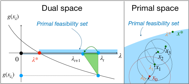
Figure 1: Primal feasibility set in primal and dual spaces, for problem $\min_{x}f(x),\text{ s.t. }g(x)\leq 0$. For primal feasibility of dual updates, we restrict the dual step sizes. For feasibility of the primal updates, we ensure the next dual update $x_{t+1}$ lies within a safety set of $x_{t}$ (circle). Here, we denote $x_{\lambda_{t}}$ as $x_{t}$ for simplicity.

As shown in Table 1, our method enjoys a substantially better sample complexity compared to current state-of-the-art. Concretely, in the case of a single smooth safety constraint, we achieve a sample complexity as $\mathcal{N}=\tilde{O}(\frac{1}{\varepsilon^{2}})$ for strongly-convex problem with stochastic gradient feedback, $\mathcal{N}=\tilde{O}(\frac{1}{\varepsilon^{4}})$ for convex problems, and $\mathcal{N}=\tilde{O}(\frac{1}{\varepsilon^{6}})$ for non-convex problems, where under $\tilde{O}(\cdot)$, we hide a multiplicative logarithmic factor. Despite the main setting of a single constraint being limiting, we can extend our approach to multiple constraints by taking a maximum over constraints and applying any smoothing procedure to the resulting constraint. Such an approach leads to a worse sample complexity by a factor of $\frac{1}{\varepsilon}$; however, in convex and strongly convex cases, it is still strictly better than the baseline. We provide a more detailed discussion in Section 6. The corresponding rates can be found in Table 1.

An advantage of our approach is that it is generic: it allows for use of any constrained optimization solver $\mathcal{A}$ on user’s choice for given type of feedback, for the internal primal steps to find $x_{t+1}$ given the fixed $\lambda_{t+1}$. Another limitation is that for convex case it is a two-cycle method (three-cycle for non-convex problems), which makes it harder to extend for online problems. Despite that, we believe our method has its own theoretical value, as it is conceptually new; feasibility during the learning was never guaranteed before for primal-dual methods.

Table 1: Sample complexity of first-order safe smooth optimization algorithms: SafeOpt (Berkenkamp et al., 2016), LB-SGD (Usmanova et al., 2023), and SafePD (this work). Here $\varepsilon$ is the target accuracy, and $d$ is the dimensionality. NLP stands for Non-Linear Programming. In SafeOpt, $\gamma(d)$ depends on the kernel, and might be exponential in $d$. The last column shows the complexity of a single iterate, for SafeOpt it requires solving a non-linear optimization sub-problem. SafePD^∗ is the extension to multiple constraints.

Method	Str-cvx	Cvx	Non-cvx	Step complexity
SafeOpt	-	-	$O\left(\frac{\gamma(d)}{\varepsilon^{2}}\right)$	NLP subproblem
LB-SGD	$\tilde{O}\left(\frac{1}{\varepsilon^{5}}\right)$	$\tilde{O}\left(\frac{1}{\varepsilon^{6}}\right)$	$\tilde{O}\left(\frac{1}{\varepsilon^{7}}\right)$	gradient step
SafePD (1 constraint)	$\tilde{O}\left(\frac{1}{\varepsilon^{2}}\right)$	$\tilde{O}\left(\frac{1}{\varepsilon^{4}}\right)$	$\tilde{O}\left(\frac{1}{\varepsilon^{6}}\right)$	gradient step
SafePD∗	$\tilde{O}\left(\frac{1}{\varepsilon^{3}}\right)$	$\tilde{O}\left(\frac{1}{\varepsilon^{5}}\right)$	$\tilde{O}\left(\frac{1}{\varepsilon^{7}}\right)$	gradient step

2 Problem Formulation

In this paper, we consider a safe learning problem:

$$\min_{x\in\mathbb{R}^{d}}\leavevmode\nobreak\ f(x) \mathcal{P}$$ ()

s.t. $$g(x)\leq 0,$$

where the objective $f:\mathbb{R}^{d}\rightarrow\mathbb{R}$ and the constraint $g:\mathbb{R}^{d}\rightarrow\mathbb{R}$ are unknown smooth possibly non-convex functions, and only can be accessed via a black-box oracle. We denote by $\mathcal{X}$ the feasible set $\mathcal{X}:=\{x\in\mathbb{R}^{d}:g(x)\leq 0\}.$ Crucially, we require that all iterates and query points are feasible, i.e., $x_{t}\in\mathcal{X}$. Importantly, since $g(\cdot)$ and, therefore, the set $\mathcal{X}$ are unknown, we need to ensure safety while exploring and learning the constrained optimizer. We define the corresponding Lagrangian function by $\mathcal{L}(x,\lambda):=f(x)+\lambda g(x)$.

Feedback

We assume $f(\cdot)$ and $g(\cdot)$ can be accessed via a noisy first-order oracle $\mathcal{O}(\cdot)$ which for any query $x\in\mathcal{X}$ returns a pair of stochastic measurements of $f$ and $g$ and their gradients respectively $(F(x),\nabla F(x))$ and $(G(x),\nabla G(x))$. We assume that these measurements are unbiased and $\sigma$- and $\hat{\sigma}$ sub-Gaussian respectively, that is, $\forall x\in\mathcal{X}$

$$\mathbb{E}\|F(x)-f(x)\|^{2}\leq\sigma^{2},\leavevmode\nobreak\ \leavevmode\nobreak\ \leavevmode\nobreak\ \leavevmode\nobreak\ \leavevmode\nobreak\ \leavevmode\nobreak\ \leavevmode\nobreak\ \mathbb{E}\|G(x)-g(x)\|^{2}\leq\sigma^{2},$$

$$\mathbb{E}\|\nabla F(x)-\nabla f(x)\|^{2}\leq\hat{\sigma}^{2},\leavevmode\nobreak\ \mathbb{E}\|\nabla G(x)-\nabla g(x)\|^{2}\leq\hat{\sigma}^{2},$$

where by $\|\cdot\|$ we denote $\ell_{2}$-norm on $\mathbb{R}^{d}$. We call a random variable $\xi$ zero-mean $\sigma$-sub-Gaussian if $\mathbb{E}\left[e^{\omega\xi}\right]\leq\text{exp}\left(\frac{\omega^{2}\sigma^{2}}{2}\right)\leavevmode\nobreak\ \forall\omega\in\mathbb{R}.$ It can also be shown using Taylor expansion that $\mathbb{E}\|\xi\|^{2}\leq\sigma^{2}$. We also assume that when we query the oracle multiple times, even at the same $x\in\mathcal{X}$, the resulting randomizations are independent of each other.

Assumptions

A function $f:\mathbb{R}^{d}\rightarrow\mathbb{R}$ is called $L$-Lipschitz continuous if $|f(x)-f(y)|\leq L\|x-y\|.$ It is called $M$-smooth if $f(x)\leq f(y)+\langle\nabla f(y),x-y\rangle+\frac{M}{2}\|x-y\|^{2}.$ It is called $\mu$-strongly-convex if $f(x)\geq f(y)+\langle\nabla f(y),x-y\rangle+\frac{\mu}{2}\|x-y\|^{2}.$ Throughout the paper we assume:

Assumption 1.

$f(x),g(x)$ are both $M_{f}$- and $M_{g}$-smooth respectively, $g(x)$ is also $L_{g}$-Lipschitz continuous on $\mathcal{X}.$

Assumption 2.

There exists a known feasible starting point $x_{0}\in\mathcal{X}$ such that $-g(x_{0})\geq\alpha>0.$

Without a safe point $x_{0}$, even the initial measurements can be unsafe. The above directly implies the Slater’s condition in the convex case. By $\alpha>0$ we denote the lower bound on the absolute value of the constraint at $x_{0}$: $\alpha\leq-g(x_{0}).$

Assumption 3.

There exists feasible $\tilde{x}\in\mathcal{X}$ such that $-g(\tilde{x})\geq\beta$ for some known $\beta>0$. If maximum value of $-g(x)$ exists, set $\beta:=\max_{x\in\mathbb{R}^{d}}\{-g(x)\}.$ Note that by definition, $\beta\geq\alpha.$

Optimality criteria and sample complexity

For problem ($\mathcal{P}$), we call $x$ an $\varepsilon$-approximate feasible solution, if $f(x)-f(x^{*})\leq\varepsilon$ and $g(x)\leq 0$. We call pair $(x,\lambda)$ an $(\varepsilon_{p},\varepsilon_{c})$-approximate KKT point, if the following holds:

$$\|\nabla_{x}\mathcal{L}(x,\lambda)\| \leq\varepsilon_{p}, (\varepsilon_{p},\varepsilon_{c})$$ (-KKT.1)

$$-g(x)\lambda \leq\varepsilon_{c}, (\varepsilon_{p},\varepsilon_{c})$$ (-KKT.2)

$$\lambda\geq 0,-g(x) \geq 0, (\varepsilon_{p},\varepsilon_{c})$$ (-KKT.3)

where $\varepsilon_{p}$ is the accuracy in the Lagrangian gradient norm, and $\varepsilon_{c}$ is the accuracy of the approximate complementarity slackness. For any algorithm $\mathcal{A}^{\prime}$, by $\mathcal{N}_{\mathcal{A}^{\prime}}(\varepsilon)$ we define a total sample complexity of $\mathcal{A}^{\prime}$ to solve a given optimization problem up to accuracy $\varepsilon$, which is a total number of oracle queries including complexity of internal algorithms.

3 Preliminaries

In this section, we introduce particular properties of dual function and safety sets, crucial for our analysis.

Duality

In the convex case, the original constrained problem is equivalent to the dual problem $\max_{\lambda\geq 0}\min_{x\in\mathbb{R}^{d}}\mathcal{L}(x,\lambda)=\max_{\lambda\geq 0}d(\lambda).$ In the above we denote by $d(\cdot)$ the dual function $d(\lambda):=\min_{x\in\mathbb{R}^{d}}\mathcal{L}(x,\lambda).$ The corresponding to $\lambda$ primal variable is denoted by $x_{\lambda}:=\arg\min_{x\in\mathbb{R}^{d}}\mathcal{L}(x,\lambda).$ Let $\lambda^{*}:=\arg\max_{\lambda\geq 0}d(\lambda)$ be the optimal dual variable. Then, we can upper bound the norm of the optimal $\lambda^{*}$:

Lemma 4.

Let Assumption 3 hold for ($\mathcal{P}$), then $\lambda^{*}\leq\Lambda:=\frac{\Delta_{f}}{\beta}$ , where $f(x)-f(x^{*})\leq\Delta_{f}$ for all $x\in\mathcal{X}$. Additionally, $\lambda^{*}\leq\frac{f(x_{0})-f(x^{*})}{-g(x_{0})}$ holds.

For the proof see Appendix B.1. In the above, $\Delta_{f}$ is a general upper bound on $f(x)-f(x^{*})\forall x\in\mathcal{X}.$ Note that if $\Delta_{f}$ is unknown, it can still be upper bounded by $\Delta_{f}:=\max_{x\in\mathcal{X}}f(x)-f(x^{*}):=f(\hat{x})-f(x^{*})\leq\|\nabla f(\hat{x})\|R+\frac{M_{f}}{2}R^{2},\text{with }\hat{x}\in\arg\max_{x\in\mathcal{X}}f(x),$ where $\|\nabla f(\hat{x})\|\leq\|\nabla f(x_{0})\|+M_{f}R$ due to the smoothness of $f$. Here, by $R$ we denote an upper bound on the initial distance to the set of optimal solutions: $\|x_{0}-x^{*}\|\leq R\leavevmode\nobreak\ ,\leavevmode\nobreak\ \forall x^{*}\in\arg\min_{x\in\mathcal{X}}f(x).$

Also, the dual problem of $\mathcal{P}$ with a strongly-convex objective $f$ is smooth:

Lemma 5.

If $f(x)$ is $\mu_{f}$-strongly-convex, and $g(x)$ is convex and $L_{g}$-Lipschitz-continuous, then the dual function $d(\lambda)$ is $\frac{2L_{g}^{2}}{\mu_{f}}$-smooth.

For the proof see Appendix B.2. Yu and Neely (2015) proved that under some rank conditions on the constraints Jacobian, the dual function is strongly-concave with some $\mu_{d}$. (See Theorem 10, Yu and Neely (2015)). For a single constraint the rank condition holds automatically. Moreover, we can prove the local strong-concavity and provide a bound on $\mu_{d}$ below.

Lemma 6.

Problem ($\mathcal{P}$) has a $\mu_{d}$-locally strongly-concave dual function with $\mu_{d}=\frac{l^{2}}{M_{f}+\lambda M_{g}}$ for all $\lambda$ such that $\|\nabla g(x_{\lambda})\|\geq l>0$. For convex $g$, it implies $\mu_{d}\geq\frac{\beta^{2}}{4R^{2}(M_{f}+\lambda M_{g})}$ for all $\lambda$ such that $g(x_{\lambda})\geq-\beta/2$, where $\beta$ is defined in Definition 3.

The proof is based on the definition of the Hessian of the dual problem, and can be found in Appendix B.3. The local strong concavity and smoothness of the dual problem allows to bound the convergence rate of our approach, where outer iterations are basically dual gradient ascent steps.

Safety set

Here, we introduce an notion of a safety region at the current point $x_{t}$, using Lipschitz continuity of the constraint. Let $\mathbb{B}^{d}(c,r)$ denote the Euclidean ball in $\mathbb{R}^{d}$ centered at $c$ with radius $r>0$. For point $x_{t}\in\mathcal{X}$ the safety region $\mathcal{S}(x_{t}):=\mathbb{B}^{d}(x_{t},\frac{-g(x_{t})}{{\color[rgb]{0,0,0}2}L_{g}})$ is the ball with center at $x_{t}$ and radius $\frac{-g(x_{t})}{{\color[rgb]{0,0,0}2}L_{g}}$, where $L_{g}$ is the Lipschitz continuity constant of $g(x)$ on $\mathcal{X}$.

Lemma 7.

Given that $x_{t}\in\mathcal{X}$ is strictly feasible, all points $x$ within the safety set $\mathcal{S}(x_{t})$ satisfy $g(x)\leq\frac{g(x_{t})}{2}<0$, implying their strict feasibility.

Proof  Indeed, from Lipschitz continuity we have for all $x\in\mathcal{S}(x_{t})$ : $g(x)-g(x_{t})\leq L_{g}\|x-x_{t}\|$, what implies $g(x)\leq g(x_{t})+L_{g}\|x-x_{t}\|\leq g(x_{t})+L_{g}\frac{-g(x_{t})}{{\color[rgb]{0,0,0}2}L_{g}}\leq\frac{g(x_{t})}{2}.$  
Often, exact measurements of $g(x_{t})$ are unknown, in this case we can use the upper bound $\hat{g}(x_{t})$ with confidence $1-\delta$ and define the corresponding approximate safety set by $\hat{\mathcal{S}}(x_{t}):=\mathbb{B}^{d}(x_{t},\frac{-\hat{g}(x_{t})}{L_{g}})$, that guarantees feasibility of $x\in\hat{\mathcal{S}}(x_{t})$ with probability $1-\delta.$

4 Strongly-Convex Problem

As the main building block of our approach, we propose a primal-dual safe method addressing strongly-convex and smooth optimization problem. Strongly-convex problem in our paper satisfies the assumption below:

Assumption 8.

The objective $f(x)$ is $\mu_{f}$-strongly-convex and $M_{f}$-smooth for some $M_{f}\geq\mu_{f}>0$. Also, the constraint function $g(x)$ is convex and $M_{g}$-smooth.

Then, the main idea of our approach can be described as follows. First, we find an initial primal-dual pair $(\check{\lambda},\check{x})$, such that $\check{x}\approx\min_{x\in\mathbb{R}^{d}}\mathcal{L}(x,\check{\lambda})$ is strictly feasible. By taking $\check{\lambda}$ big enough, we guarantee that any descent method $\check{\mathcal{A}}$ applied to $\arg\min_{x\in\mathbb{R}^{d}}\mathcal{L}(x,\check{\lambda})$ starting from $x_{0}\in Int(\mathcal{X})$ does also imply feasibility of its iterates, including feasibility of $\check{x}.$ We set $(x_{1},\lambda_{1})=(\check{x},\check{\lambda})$. Next, we iteratively update pair $(\lambda_{t},x_{t})$ as follows:

1. We iteratively decrease the dual variable (dual iteration) $\lambda_{t+1}\leftarrow\max\{\lambda_{t}-\frac{-\mu g(x_{t})}{{\color[rgb]{0,0,0}8}L_{g}^{2}},0\}$. This update corresponds to the dual gradient ascent with the step-size $\gamma=\frac{\mu}{{\color[rgb]{0,0,0}8}L_{g}^{2}},$ which guarantees that the corresponding primal solution $x_{\lambda_{t+1}}:=\arg\min_{x\in\mathbb{R}^{d}}\mathcal{L}(x,\lambda_{t+1})$ lies in the approximate safety region $\hat{\mathcal{S}}(x_{t})$ around the last update $x_{t}$.

2. We solve the primal problem (primal iteration) of the corresponding dual variable $x_{t+1}\leftarrow\arg\min_{x\in\hat{\mathcal{S}}(x_{t})}\mathcal{L}(\cdot,\lambda_{t+1})$ constrained to the safety region, up to accuracy $\eta_{t}>0$, i.e., $\mathcal{L}(x_{t+1},\lambda_{t+1})-\mathcal{L}(x_{\lambda_{t+1}},\lambda_{t+1})\leq\eta_{t}.$ This can be done safely using any projection descent method, or any approach that preserves feasibility subject to a ball constraint $\hat{\mathcal{S}}(x_{t})$.

This way, we guarantee a continuous sequence of primal subproblems such that the path between the new $x_{t+1}$ and the past $x_{t}$ lies fully in the safety set of $x_{t}$. Our approach for the Strongly-Convex case is depicted in Algorithm 1. We set the required primal accuracy to be $\eta_{t}:=\begin{cases}\frac{\mu_{f}\hat{g}(x_{t})^{2}}{128L_{g}^{2}},&\text{ if }-\hat{g}(x_{t})\lambda_{t+1}>\varepsilon_{c}\\ \min\{\frac{\mu_{f}}{M_{L}}\varepsilon_{p}^{2},\frac{\varepsilon}{2}\},&\text{ if }-\hat{g}(x_{t})\lambda_{t+1}\leq\varepsilon_{c}\end{cases}$ and prove it is enough in the following sections. The second case corresponds to the accuracy of the last primal step $\eta_{T}.$ In the above, by $\eta_{t}$ we denote accuracy of solving the primal subproblem at step $t$. By $\check{\eta}$ we denote accuracy of solving the initial primal subproblem.

Algorithm 1 Strongly-Convex Safe Algorithm (SCSA)

0:  $x_{0}:-g(x_{0})\geq\alpha>0,$ $\beta>0$, $L_{g},$ $\mu_{f}$, $M_{f},M_{g}>0,$ $\Delta_{f}>0,$ $\{\epsilon_{t}\}_{t=0}^{T}$, $\{\eta_{t}\}_{t=0}^{T}$. Set $\check{\lambda}\leftarrow\frac{\Delta_{f}}{\alpha}.$

0:  Preliminary step: $\check{x}\leftarrow\check{\mathcal{A}}(\mathcal{L}(\cdot,\check{\lambda}),\mathbb{R}^{d},x_{0})$ (up to acc. $\check{\eta}\leq\frac{\mu_{f}\alpha^{2}}{8L_{g}^{2}}$), and set $(x_{1},\lambda_{1})\leftarrow(\check{x},\check{\lambda})$

 for $t\in\{1,\ldots,T\}$  do

   Estimate $\epsilon_{t}$-approximate upper bound on $g(x_{t})$ using a minibatch with $n_{t}:=\frac{4\sigma^{2}}{\epsilon_{t}^{2}}\ln\frac{T}{\delta}$ samples:

$$\hat{g}(x_{t}):=\frac{\sum_{i=1}^{n_{t}}G_{i}(x_{t})}{n_{t}}+\frac{\sigma}{\sqrt{n_{t}}}\sqrt{\ln\frac{T}{\delta}}$$

   Safety set: $\hat{\mathcal{S}}(x_{t})\leftarrow\mathbb{B}^{d}(x_{t},\frac{-\hat{g}(x_{t})}{L_{g}})$

   Dual update: $\lambda_{t+1}\leftarrow\max\{\lambda_{t}+\gamma\hat{\nabla}d(\lambda_{t}),0\}$, where $\gamma=\frac{\mu_{f}}{{\color[rgb]{0,0,0}8}L_{g}^{2}}$ and $\hat{\nabla}d(\lambda_{t})=\hat{g}(x_{t})$

   Primal update: $x_{t+1}\leftarrow\mathcal{A}(\mathcal{L}(\cdot,\lambda_{t+1}),\hat{\mathcal{S}}(x_{t}),x_{t})$, up to accuracy $\eta_{t}$

   If $-\hat{g}(x_{t})\lambda_{t+1}\leq\varepsilon_{c}$ break

 end for

  $(x_{T},\lambda_{T})$

Internal algorithms

By algorithm $\mathcal{A}(f,\mathcal{C},x_{0})$ we denote an optimization procedure with known simple constraint set $\mathcal{C}$, for minimizing $\min f(x)$ s.t. $x\in\mathcal{C}$, where $f$ is $M$-smooth and $\mu$-strongly-convex, the procedure is starting from $x_{0}\in\mathcal{C}$ and all the updates are feasible $x_{t}\in\mathcal{C}$. For internal algorithm $\mathcal{A}$ we can use any algorithm ensuring feasible iterations with known feasibility set $\hat{\mathcal{S}}(x_{t})$, e.g., the projected gradient descent: $\mathcal{A}_{PGD}(\mathcal{L}(\cdot,\lambda_{t+1}),\hat{\mathcal{S}}(x_{t}),x_{t})$ or projected stochastic gradient descent $\mathcal{A}_{SGD}(\mathcal{L}(\cdot,\lambda_{t+1}),\hat{\mathcal{S}}(x_{t}),x_{t}).$ Adam or other momentum-based algorithms can be used too. By $\check{\mathcal{A}}$ we denote an optimization method ensuring descent at every step.

Estimating a constraint value.

Note that in order to estimate the safety set at point $x$, we need to estimate the constraint value $g(x)$. The accuracy of this estimation is limited by the noise level of measurements. We can decrease this error by taking a minibatch of several noisy samples of $g(x)$ at the required point $x$. Let us denote by $\epsilon_{t}$ the required approximation accuracy of the constraint value estimation at iteration $t$ with high probability $\mathbb{P}\{\forall t\leq T:g(x_{t})-\hat{g}(x_{t})\leq\epsilon_{t}\}\geq 1-\delta.$ As we later show in Theorem 13, estimating constraint values $g(x_{t})$ up to accuracy $\epsilon_{t}=O(\varepsilon)$ is enough for safe convergence to $\varepsilon$-approximate solution. In Step 1., we approximate $g(x_{t})$ by using a minibatch of $n_{t}$ samples. Note that from standard concentration inequalities for sub-Gaussian random variables, we have $\mathbb{P}\left\{\left|\frac{\sum_{i=1}^{n_{t}}G_{i}(x_{t})}{n_{t}}-g(x_{t})\right|\leq\frac{\sigma}{\sqrt{n_{t}}}\sqrt{\ln\frac{1}{\delta}}\right\}\geq 1-\delta$. Therefore, by taking $n_{t}\geq\frac{\sigma^{2}}{\epsilon_{t}^{2}}\ln\frac{T}{\delta}$ ensures that $\mathbb{P}\{\forall t\leq T:g(x_{t})-\hat{g}(x_{t})\leq\epsilon_{t}\}\geq 1-\delta.$

In the next three subsections, we provide the theoretical justification of our procedure. In particular, we provide the safety and convergence guarantees, and bound the sample complexity.

4.1 Safety

We split this section into two parts, describing separately safety of finding the initial pair $(\check{x},\check{\lambda})$ and safety of the transition $(x_{t},\lambda_{t})\rightarrow(x_{t+1},\lambda_{t+1}).$

Safe dual initialization

First, we prove the safety of obtaining $(\check{x},\check{\lambda})$ in a safe way starting from $x_{0}$. For that, one can set $\check{\lambda}\geq\frac{\Delta_{f}}{\beta}$, and use any descent method to minimize $\min_{x\in\mathbb{R}^{d}}\mathcal{L}(x,\check{\lambda}).$

Lemma 9.

Let $\check{\lambda}=\frac{\Delta_{f}}{\alpha}\geq\frac{f(x_{0})-\min_{x}f(x)}{-g(x_{0})}.$ Then, all iterates $x_{t}$ of any descent method for $\mathcal{L}(x,\lambda)$ starting at $x_{0}$ would guarantee feasibility of the iterates $g(x_{t})\leq 0.$

For the proof see Appendix B.4. Specifically, we can use SGD with an appropriate minibatch size to estimate the gradients well enough, to guarantee descent at every step with high probability in the following Lemma 10. For its proof see Appendix D.1.

Lemma 10.

Let us use mini-batch SGD $\check{\mathcal{A}}_{mSGD}$ during the initial stage of SCSA (Alg. 1) with properly chosen mini-batch size $n_{0}(\tau)=\frac{4\sigma^{2}}{\|\nabla\tilde{\mathcal{L}}(x_{\tau-1},\check{\lambda})\|^{2}}$ and step-size $\gamma_{\tau}\leq\frac{1}{M_{f}+\check{\lambda}M_{g}}.$ Then, it ensures descent at every step, and converges to $\check{\eta}$-optimal point after $\mathcal{T}=O(\log\frac{1}{\check{\eta}})$ iterates, with total sample complexity $\mathcal{N}_{0}=\tilde{O}(\frac{1}{\check{\eta}^{2}})$.

Safe transition

Next, we discuss a safe transition from $(x_{t},\lambda_{t})$ to $(x_{t+1},\lambda_{t+1})$, given that $(x_{t},\lambda_{t})$ are feasible. Consider the dual problem $d(\lambda)$, where $\lambda$ is scalar in the case of a single constraint. As shown at Figure 2, the optimal $\lambda^{*}$ corresponds to the maximum of $d(\lambda)$, i.e., $\|\nabla d(\lambda^{*})\|=0$ if the solution is on the boundary, otherwise $\lambda^{*}=0$. Recall that $\|\nabla d(\lambda)\|=g(x_{\lambda})$, which should be negative for $x_{\lambda}\in\mathcal{X}.$ Concavity of $d(\lambda)$ implies monotonously decreasing $\nabla d(\lambda).$ Therefore, indeed, $\lambda\geq\lambda^{*}$ corresponds to the primal feasibility region in the dual space. Secondly, note that $\nabla d(\lambda)$ growth is limited by the smoothness bound of $d(\lambda).$ Hence, we can control that $g(x_{\lambda_{t}})$ stays in the negative region by controlling the dual step size. But, just guaranteeing the next $x_{\lambda_{t}}$ is safe is not enough, since we should also find a way to safely transit from $x_{t}$ to $x_{t+1}$. In order to do that, we restrict the step size even more, to guarantee that $x_{\lambda_{t+1}}\in\hat{\mathcal{S}}(x_{t}).$

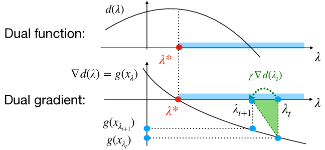
Figure 2: Primal feasibility of the dual iterates

Lemma 11.

Let $\lambda_{t}$ correspond to a feasible point $x_{\lambda_{t}}.$ Let the dual step be bounded by $\lambda_{t}-\lambda_{t+1}\leq\frac{-\mu_{f}\hat{g}(x_{t})}{{\color[rgb]{0,0,0}8}L_{g}^{2}}$, as defined in Step 3 of Alg. 1. Also, let $x_{t}$ be an $\eta_{t}$-accurate solution of $\min_{x\in\mathbb{R}^{d}}\mathcal{L}(x,\lambda_{t})$ with $\eta_{t}\leq\frac{\mu_{f}(-\hat{g}(x_{t-1}))^{2}}{{\color[rgb]{0,0,0}32}L_{g}^{2}}.$ Then, $\|x_{\lambda_{t+1}}-x_{t}\|\leq\frac{-\hat{g}(x_{t})}{{\color[rgb]{0,0,0}2}L_{g}}$, that is, $x_{\lambda_{t+1}}\in\hat{\mathcal{S}}(x_{t})$ with probability $1-\delta$.

The full proof can be found in Appendix B.5. This lemma combined with the way the primal updates are done $x_{t+1}\leftarrow\arg\min_{x\in\hat{S}(x_{t})}\mathcal{L}(x,\lambda_{t+1})$ directly implies safety of SCSA (Alg. 1). Indeed, by using a feasible algorithm $\mathcal{A}(\mathcal{L}(\cdot,\lambda_{t+1}),\hat{\mathcal{S}}(x_{t}),x_{t})$ with projections onto the safety set $\hat{\mathcal{S}}(x_{t})$, we ensure that all the inner iterations are safe, including the last one $x_{t+1}$. And for the very first initialisation run of algorithm $\check{\mathcal{A}}$, the updates are feasible as long as $\check{\mathcal{A}}$ is a descent algorithm. This implies our safety result:

Theorem 12.

Under Assumptions 2, 1, 3, and 8, SCSA (Alg. 1) guarantees that with probability $\geq 1-\delta$, all oracle queries for iterates $t=1,\ldots,T$ are safe, i.e, $g(x_{t})\leq 0$ and $g(x_{t,\tau})\leq 0$ for all steps $\{x_{t,\tau}\}_{\tau=1,\ldots,\mathcal{T}}$ of internal algorithms $\mathcal{A}$ and $\check{\mathcal{A}}$.

Moreover, note that $x_{t+1}\approx\arg\min_{x\in\hat{\mathcal{S}}(x_{t})}\mathcal{L}(x,\lambda_{t+1})=\arg\min_{x\in\mathbb{R}^{d}}\mathcal{L}(x,\lambda_{t+1})$ since $x_{\lambda_{t+1}}\in\hat{\mathcal{S}}(x_{t})$ by Lemma 11. The above fact allows us to guarantee that our safe primal updates restricted to a safe region still form a sequence of primal-dual pairs $(x_{t},\lambda_{t})$.

4.2 Sample complexity

In this section, we derive the sample complexity of the SCSA (Alg. 1). For that, we analyze the number of outer iterates, and sample complexity of the inner algorithms. We exploit the fact that the outer iterates correspond to the gradient ascent of a strongly-concave dual problem, therefore providing a linear convergence.

Theorem 13.

Consider problem ($\mathcal{P}$) under Assumptions 2, 1, 3, and 8. Let the primal sub-problems of SCSA (Alg. 1) be solved with accuracy

$$\eta_{t+1}=\begin{cases}\frac{\mu_{f}\hat{g}(x_{t})^{2}}{128L_{g}^{2}},&\text{ if }-\hat{g}(x_{t})\lambda_{t+1}>\varepsilon_{c}\\ \min\{\frac{\mu_{f}}{M_{L}^{2}}\varepsilon_{p}^{2},\frac{\varepsilon}{2}\},&\text{ if }-\hat{g}(x_{t})\lambda_{t+1}\leq\varepsilon_{c}\end{cases},$$

and constraint measurements be taken up to accuracy $\epsilon_{t}\leq\frac{-\hat{g}(x_{t-1})}{8}$ with probability $1-T\delta.$ Then, the algorithm stops after at most $T=O(\frac{\check{\lambda}}{\beta}+\frac{L_{g}^{2}R^{2}}{\beta^{2}}\frac{M_{f}}{\mu_{f}}\log\frac{\check{\lambda}^{2}}{\mu_{f}\varepsilon_{c}})$ outer iterations of SCSA (Alg. 1) with probability $1-\delta$ and outputs an $(\varepsilon_{p},\varepsilon_{c})$-approximate KKT point, i.e., $\|\nabla\mathcal{L}(x_{T},\lambda_{T})\|\leq\varepsilon_{p},\leavevmode\nobreak\ \lambda_{T}(-g(x_{T}))\leq\varepsilon_{c}.$ Moreover, given $\varepsilon_{c}\leq\varepsilon/2$, $\eta_{T}\leq\varepsilon/2$, we have $f(x_{T})-f(x^{*})\leq\varepsilon.$

Proof  For the full proof see Appendix C. Here we provide a short proof sketch. The outer steps of our algorithm $\lambda_{t+1}\leftarrow\max\{\lambda_{t}-\frac{(-\hat{g}(x_{t}))\mu_{f}}{{\color[rgb]{0,0,0}8}L_{g}^{2}},0\}$, form a projected gradient ascent for the dual problem $d(\lambda)$ with a constant step size and approximate gradient. Moreover, $\forall t>0$: $\lambda_{t}$s are only decreasing: $\lambda_{t+1}\leq\lambda_{t}$. Also, note that the dual problem $d$ is locally-strongly-concave at the region $\Omega_{\lambda}:=\{\lambda\in\mathbb{R}:g(x_{\lambda})\geq\frac{-\beta}{2}\}$, thus implying fast convergence in that region.

Firstly, we show that the method’s dual updates $\lambda_{t}$ can be outside of $\Omega_{\lambda}$ only for a finite number of steps $T_{0}$. Indeed, since outside of $\Omega_{\lambda}$ the gradient norm is lower bounded by a constant $\|\nabla d(\lambda)\|=-g(x_{\lambda})\geq\beta/2$, we make at least a constant progress at each step, until reaching $\Omega_{\lambda}$ in $T_{0}$ steps constant in $\varepsilon_{c}$, bounded by $T_{0}\leq\frac{8L_{g}^{2}}{\mu_{f}}\frac{\check{\lambda}}{\beta}.$ If the method stops earlier by reaching $\lambda_{t}=0$, then $T=T_{0}$.

Secondly, inside this region $\Omega_{\lambda}$ we prove the linear convergence rate using standard techniques and careful disturbance analysis. In particular, by using the bounds on $\epsilon_{t}$ and $\eta_{t}$ from the theorem conditions, we show that the estimate of the dual gradient $\|\hat{\nabla}d(\lambda_{t})-\nabla d(\lambda_{t})\|\leq\frac{\|\nabla d(\lambda_{t})\|}{2}$ with probability $1-\delta$ for all $t>0$ (using Boole’s inequality), which is enough to have a linear convergence rate. That is, $(\lambda_{t+1}-\lambda_{*})\leq\left(1-\frac{\mu_{f}\mu_{d}}{16L_{g}^{2}}\right)^{t-T_{0}}\check{\lambda}$. We also show that $-\hat{g}(x_{t})\lambda_{t+1}\leq\max\left\{\bar{G},\frac{4L_{g}^{2}\check{\lambda}}{\mu_{f}}\right\}(\lambda_{t+1}-\lambda_{*})$, where $-\hat{g}(x_{t})\leq\bar{G}$ for all $t$ (which holds for $\bar{G}=2\hat{g}(\check{x})$). Note that until stopping $-\hat{g}(x_{t})\lambda_{t+1}>\varepsilon_{c}$, what implies that $\varepsilon_{c}\leq-\hat{g}(x_{t})(\lambda_{t+1}-\lambda_{*})\leq\max\left\{\bar{G}\check{\lambda},\frac{4L_{g}^{2}\check{\lambda}^{2}}{\mu_{f}}\right\}\left(1-\frac{\mu_{f}\mu_{d}}{16L_{g}^{2}}\right)^{t-T_{0}}.$ From the above we can directly upper bound the maximal number of steps before stopping:

$$T\leq \frac{8L_{g}^{2}\check{\lambda}}{\beta\mu_{f}}+\frac{16L_{g}^{2}}{\mu_{d}\mu_{f}}O\left(\ln\frac{\check{\lambda}^{2}}{\mu_{f}\varepsilon_{c}}\right).$$ (1)

Using $\mu_{d}\geq\frac{\beta^{2}}{4R^{2}M_{L}},$ we get the bound from the theorem. Using the relation of primal optimality to the Lagrangian optimality, we show that given $\varepsilon_{c}\leq\varepsilon/2$, $\eta_{T}\leq\varepsilon/2$, we have $f(x_{T})-f(x^{*})\leq\varepsilon.$ The expression for iteration complexity in Eq. (1) gives us the linear convergence rate for the dual iterations.  

Finally, we can guarantee the following sample complexity.

Corollary 14.

Consider stochastic oracle with gradient variance $\hat{\sigma}^{2}>0$ and value variance $\sigma^{2}>0.$ Then, the method requires $\mathcal{N}(\varepsilon)=\mathcal{N}_{0}(\check{\eta})+O\left(\frac{L_{g}^{2}}{\beta^{2}}\frac{M_{f}}{\mu_{f}}\log\frac{1}{\varepsilon}\right)\left(\mathcal{N}_{\mathcal{A}}(\min\eta_{t})+n_{t}(\epsilon_{t})\right)$ oracle calls to get $f(x_{T})-f(x^{*})\leq\varepsilon$, where $\mathcal{N}_{\mathcal{A}}(\eta_{t})$ is the sample complexity of the internal algorithm. For $\mathcal{A}\leftarrow\mathcal{A}_{SGD}$ and the conditions of $\check{\eta},\eta_{t},\epsilon_{t},n_{t}$, the total sample complexity is

$$\mathcal{N}(\varepsilon)=O\left(\frac{\check{\lambda}}{\beta}+\frac{M_{f}}{\mu_{f}}\frac{R^{2}}{\beta^{2}}\log\frac{1}{\varepsilon}\right)O\left(\frac{\sigma^{2}}{\varepsilon^{2}}+\frac{(L+\hat{\sigma})^{2}}{\mu_{f}\varepsilon^{2}}\right).$$

For the proof see Appendix C.3.

4.3 General Smooth and Convex Case

Here, we consider the case where the objective and constraint are smooth and convex, but not necessarily strongly-convex. In this case, one can regularize the objective in order to make it strongly-convex. In particular, we can formalize the algorithm as follows:

Algorithm 2 SCSA (Alg. 1) for convex problems

0: Initialization: Feasible starting point $x_{0}$: $g(x_{0})\leq-\beta<0$, regularization parameter $\mu_{f}=\frac{\varepsilon}{R^{2}}>0$.

0:  Define $\hat{\mathcal{P}}:\min f(x)+\frac{\mu_{f}}{2}\|x-x_{0}\|^{2}\text{ s.t. }g(x)\leq 0.$

0:  $(x_{T},\lambda_{T})\leftarrow SCSA(\hat{\mathcal{P}},x_{0})$

Theorem 15.

Consider problem ($\mathcal{P}$) under Assumptions 2, 1, 3, and let $f(\cdot)$ and $g(\cdot)$ be convex. Let $x_{0}$ be a starting vector, such that $\|x_{0}-x^{*}\|\leq R$, where $x^{*}=\arg\min_{x\in\mathcal{X}}f(x)$. Then, applying Algorithm 1 to a regularized problem $\min f(x)+\frac{\mu_{f}}{2}\|x-x_{0}\|^{2}$ s.t. $g(x)\leq 0$ with $\mu_{f}=\varepsilon/R^{2}$ produces an output $x_{T}$ satisfying $f(x_{T})-\min_{x\in\mathcal{X}}f(x)\leq\varepsilon$ in a total sample complexity of $\mathcal{N}(\varepsilon)=O(\frac{1}{\varepsilon^{4}})$, with probability $1-\delta.$ Also, all iterates are safe with probability $1-\delta.$

For the proof see Appendix C.2.

5 Non-convex Case

In this section, we address the setting of safe optimization of general non-convex and smooth objective and constraints; our performance measure is the an $(\varepsilon_{p},\varepsilon_{c})$-approximate KKT condition. First, let us make an additional regularity assumption, which is an extension of Mangasarian-Fromovitz Constraint Qualification (MFCQ):

Assumption 16.

There exists $\theta\in(0,\frac{\beta}{2}]$ such that for any point in $\{x\in\mathcal{X}|g(x)\geq-\theta\}$ there exists a constant $l>0$, such that $\|\nabla g(x)\|\geq l.$

The classic MFCQ (Mangasarian and Fromovitz, 1967) is the regularity assumption on the constraints, guaranteeing that they have a uniform descent direction for all constraints at a local optimum. 16 guarantees $g(x)$ is decreasing towards the middle of the set at all points $\theta$-close to the boundary; it is the same as in Usmanova et al. (2023).

To address the non-convex case, first note that smoothness of $f(x)$ and $g(x)$ implies their weak convexity. That is, there exists such constant $\rho_{f}>0$ such that $f(x)+\frac{\rho_{f}}{2}\|x-x_{0}\|^{2}$ becomes convex, same with the constraint function. Then, we propose to use smoothing technique with the moving regularizer, inspired by Zhang et al. (2020). In particular, at each step $k$ consider regularized problem:

$$\min_{x\in\mathbb{R}^{d}}\leavevmode\nobreak\ f(x)+\frac{\rho_{f}}{2}\|x-x_{k-1}\|^{2}, \mathcal{P}_{x_{k-1}}$$ ()

s.t. $$g(x)+\frac{\rho_{g}}{2}\|x-x_{k-1}\|^{2}\leq 0$$

with the corresponding Lagrangian

$$\mathcal{K}_{x_{k-1}}(x,\lambda):=f(x)+\frac{\rho_{f}}{2}\|x-x_{k-1}\|^{2}+\lambda\left(g(x)+\frac{\rho_{g}}{2}\|x-x_{k-1}\|^{2}\right)$$

with regularizer parameters $\rho_{f}>M_{f}$ and $\rho_{g}>M_{g}$, so that both regularized objective and constraint functions are $\mu_{i}=\rho_{i}-M_{i}$-strongly convex and $\rho_{i}+M_{i}$-smooth for $i\in\{f,g\}$. Note that $\mathcal{K}_{x_{k-1}}(\cdot,\lambda)$ is also $\mu_{K}=\rho_{f}-M_{x}+\lambda(\rho_{g}-M_{g})$ strongly-convex, and $M_{K}=\rho_{f}+M_{f}+\lambda(\rho_{g}+M_{g})$-smooth respectively.

We define the detailed updates in Algorithm 3. Here, $\beta_{k}$ is a lower bound $\beta$ for problem $\mathcal{P}_{x_{k-1}}$, i.e., $-\min_{x\in\mathbb{R}^{d}}\{g(x)+\frac{\rho_{g}}{2}\|x-x_{k-1}\|^{2}\}\geq\beta_{k}:=-\hat{g}(x_{k-1})$, and $\text{SCSA}(\mathcal{P}_{x_{k-1}})$ means SCSA (Alg. 1) applied to problem $\mathcal{P}_{x_{k-1}}$, and initialized directly with primal-dual pair $(\check{x}_{k},\check{\lambda}_{k})$.

Algorithm 3 Safe Primal-Dual Method (SafePD)

0: Preliminary step: Set $\check{\lambda}_{1}\leftarrow\frac{\Delta_{f}}{-\hat{g}(x_{0})}$

 for $k\in\{1,\ldots,K\}$  do

   $\check{x}_{k}\leftarrow\check{\mathcal{A}}(\mathcal{K}_{x_{k-1}}(\cdot,\check{\lambda}_{k}),\mathbb{R}^{d},x_{k-1})$ (to $\check{\eta}_{k}\leq\frac{\mu_{f}\beta_{k}^{2}}{8L_{g}^{2}}$)

   $(x_{k},\lambda_{k})\leftarrow\text{SCSA}(\mathcal{P}_{x_{k-1}})$, Alg. 1 init. at $(\check{x}_{k},\check{\lambda}_{k})$, and solved up to accuracy $(\varepsilon_{p},\varepsilon_{c})$

   If $\|x_{k-1}-x_{k}\|\leq\min\left\{\frac{{\color[rgb]{0,0,0}\varepsilon_{p}}}{\rho_{f}+\check{\lambda}_{k}\rho_{g}},\sqrt{\frac{2\varepsilon_{c}}{\check{\lambda}_{k}\rho_{g}}}\right\}$ then break

   $\hat{\lambda}_{k+1}\leftarrow 2\lambda_{k}+\frac{\rho_{f}}{\rho_{g}}+\frac{\eta_{k}}{-g(x_{k})}+\frac{\hat{\eta}_{k+1}}{-g(x_{k})}$

 end for

 Return: $(x_{K},\lambda_{K})$

Note that for sub-problem $\mathcal{P}_{x_{k-1}}$, we need $\check{\lambda}_{k}$ to be big enough that $g(\check{x}_{k})+\frac{\rho_{g}}{2}\|\check{x}_{k}-x_{k-1}\|^{2}\leq 0$, i.e., $x_{\check{\lambda}_{k}}$ is feasible subject to a regularized constraint. It appears that we can set $\check{\lambda}_{k}$ according to Step 1 using the relation of the subsequent subproblems. This provides us with a less conservative warm start, compared to the original SCSA (Alg. 1) initialization that would require $\check{\lambda}_{k}\geq\frac{f(x_{k-1})-\min_{x\in\mathcal{X}_{k}}f(x)}{-g(x_{k-1})}.$ Then, we can obtain the following convergence and sample complexity guarantees, while ensuring safety of all the updates.

Theorem 17.

Consider problem ($\mathcal{P}$) under Assumptions 2, 1, 3 with non-convex objective and constraint, and let Assumption 16 hold for some constant $\theta>0$. Then, Algorithm 3 stops after at most $K=O\left(\frac{1}{\varepsilon^{2}}\right)$ outer iterations reaching $(\varepsilon,\varepsilon)$-approximate KKT point with probability $1-\delta K$. In total, it requires $\mathcal{N}=O\left(\frac{1}{\varepsilon^{6}\theta}\right)$ samples. Moreover, all iterates are feasible with probability $1-\delta K$.

The proof can be found in the Appendix D.

6 Extension to Multiple Safety Constraints

Extending the method to multiple constraints $g_{i}(x)\leq 0\forall i\in\{1,\ldots,m\}$ is possible by replacing them with the max of all the constraints $g(x):=\max\{g_{i}(x)\}$ and applying any smoothing technique to the resulting function $g(x)$, such as randomized smoothing (Duchi et al., 2012). The convergence rate however worsens by a factor of $\frac{1}{\varepsilon}$ due to trade-off between the approximation quality and and smoothness constant. Indeed, the smoothed constraint $g_{\nu}(x)$ with parameter $\nu>0$ is $O(\nu)$-approximation of the original constraint $g$ and it is $M_{\nu}$ smooth with $M_{\nu}=O(\frac{1}{\nu}).$ (Duchi et al., 2012) Therefore, we need $\nu=O(\varepsilon_{c})$ to guarantee the required solution accuracy $-g(x)\lambda\leq\varepsilon_{c}$. Then, local strong concavity of the dual function $\mu_{d}=\frac{l^{2}}{M_{f}+\lambda M_{\nu}}=\Omega(\varepsilon_{c})$. That is, the total complexity is increased to $T=\tilde{O}(\frac{1}{\varepsilon^{3}})$ for strongly convex case, and $N=\tilde{O}(\frac{1}{\varepsilon^{5}})$ for convex case, and $N=\tilde{O}(\frac{1}{\varepsilon^{7}})$ for non-convex case. Note that these bounds are still better than the previous bounds, for strongly-convex and convex cases, and similar to the baseline for non-convex case.

7 Empirical Evaluations

We compare LB-SGD (Usmanova et al., 2020) and SCSA (Alg. 1) on a synthetic strongly-convex problem with black-box stochastic feedback. In particular, we consider $\min\|x-x_{0}\|^{2},\text{ s.t.}\|Ax-b\|^{2}-4\leq 0,$ with $A=[[I_{d-1},\bar{0}],[0,..,0,2]],b=[0,...,0,1]$ and $x_{0}=[0,..,0,5].$ We consider noisy zeroth-order feedback with standard deviation $\sigma=0.01,0.1$ and dimension $d=2$. The shady area is the area between the max. and min. values over 10 runs. The gradients are approximated by finite differences, similarly to Usmanova et al. (2023). Our experiments demonstrate sensitivity of the LB-SGD to the increasing noise level, compared to our method. Note that when the noise is very small $\sigma\in{0.01}$, the setting is very close to the noise-free setting, for which SGD used in our method is non-optimal. For larger $\sigma=0.1$, the clear improvement can be seen. From the confidence-interval shades, one can also see SafePD is more stable. The complexity of SafePD can also be improved to $O\left(\log^{2}\frac{1}{\epsilon}\right)$ for the strongly-convex problems in the exact information case, since linear convergence can be achieved for the internal problems.

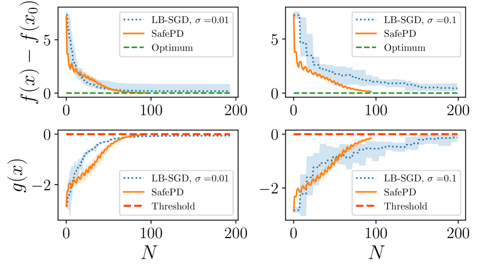
Figure 3: Comparison of SafePD (SCSA, Algorithm 1), and LB-SGD.

See Appendix A for non-convex experiments. Note that the experiments are only illustrative and the main focus of the paper is theoretical.

Appendix A Non-Convex Experiments

Here, we demonstrate the performance of our method compared to LB-SGD on the following non-convex problem of minimising inverted Gaussian over a quadratic constraint.

$$\min_{x} \exp^{-4\|x\|^{2}_{2}}$$ (2)

s.t. $$0.2\|x-x_{0}\|^{2}_{2}+10.*(x[1]-x_{0}[1])^{2}\leq r^{2}$$ (3)

with $r=0.5$, $x_{0}=\frac{1}{\sqrt{d}}[1,\ldots,1],$ and $x[1]$ is the second component of vector $x$.

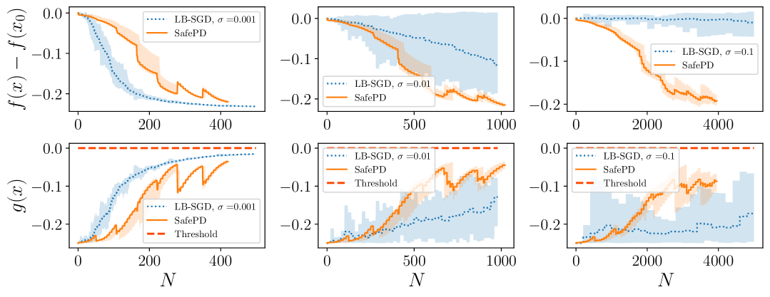
Figure 4: Comparison of SafePD (Alg. 3), and LB-SGD, on a non-convex problem.

Here, we again observe that LB-SGD with higher noise gets less stable and slower in practice. The goal of our experiments is to demonstrate sensitivity of the LB-SGD to increasing the noise level, compared to our method. Note that when the noise variance compared to the target accuracy is very small $\sigma\in{0.001,0.01}$, the given settings are very close to the noise-free setting. In the noise-free setting, the sample complexity of LB-SGD is $O\left(\frac{1}{\epsilon^{2}}\right)$ gradient steps for strongly-convex case, and $O\left(\frac{1}{\epsilon^{3}}\right)$ gradient steps for non-convex case, whereas for non-convex SafePD according to Corollary 14, the sample complexity is still $O\left(\frac{1}{\epsilon^{2}}\right)$ for the strongly-convex case and $O\left(\frac{1}{\epsilon^{6}}\right)$ for the non-convex case, since in the experiments we use SGD for the internal optimization, which is non-optimal for noise-free setting. However, note that the complexity of SafePD can be improved to $O\left(\log^{2}\frac{1}{\epsilon}\right)$ for the strongly-convex problems, $O\left(\frac{1}{\epsilon^{4}}\right)$ for non–convex problems in the exact information case, since SGD can be replaced then with a more efficient internal optimization algorithm achieving linear convergence rate in the exact information case. We do not use it in the experiments for consistency.

For the case of a higher noise level, we observe that $O\left(\frac{1}{\epsilon^{6}}\right)$ sample complexity of SafePD clearly outperforms $O\left(\frac{1}{\epsilon^{7}}\right)$ sample complexity of LB-SGD in practice, what confirms our theoretical findings. And it can also be seen from the confidence-interval shades, that our method is much more stable.

Appendix B Additional Proofs

B.1 Proof of Lemma 4

Lemma 18.

There exists a feasible point $\tilde{x}\in\mathcal{X}$ such that $-g(\tilde{x})\geq\beta>0,$ and $\Delta_{f}:=\max_{x\in\mathcal{X}}\{f(x)-f(x^{*})\}.$ Then, $\lambda^{*}\leq\frac{\Delta_{f}}{\beta}.$

Proof  Let $(x^{*},\lambda^{*})=\min_{x\in\mathcal{X}}\max_{\lambda\geq 0}\mathcal{L}(x,\lambda).$ Then, for feasible point $\tilde{x}$ we have $f(\tilde{x})-f(x^{*})\geq\lambda^{*}(-g(\tilde{x}))$, that follows directly from $\mathcal{L}(\tilde{x},\lambda^{*})\geq\mathcal{L}(x^{*},\lambda^{*}).$ It implies $\lambda^{*}$ is upper bounded by $\lambda^{*}\leq\frac{f(\tilde{x})-f(x^{*})}{-g(\tilde{x})}\leq\frac{\Delta_{f}}{\beta}.$  

B.2 Proof of Lemma 5

Lemma 19.

If $f(x)$ is $\mu_{f}$-strongly-convex, and $g(x)$ is convex and $L_{g}$-Lipschitz-continuous, then the dual function $d(\lambda)$ is $\frac{2L_{g}^{2}}{\mu_{f}}$-smooth.

Proof  Since for every $\lambda>0$ the minimizer of $\min_{x\in\mathbb{R}^{d}}\mathcal{L}(x,\lambda)$ is unique $x_{\lambda}^{*}$, the dual function is differentiable with $\nabla d(\lambda)=g(x_{\lambda}^{*}).$ Next, due to the Lipschitz continuity, we have

$$|g(x_{\lambda_{1}}^{*})-g(x_{\lambda_{2}}^{*})|\leq L_{g}\|x_{\lambda_{1}}^{*}-x_{\lambda_{2}}^{*}\|.$$

$$|g(x_{\lambda_{1}}^{*})-g(x_{\lambda_{2}}^{*})|^{2}\leq L_{g}^{2}\|x_{\lambda_{1}}^{*}-x_{\lambda_{2}}^{*}\|^{2}$$

Then, note that due to $\mu_{f}$-strong convexity of $\mathcal{L}(\cdot,\lambda_{1})$, we have:

$$\frac{\mu_{f}}{2}\|x_{\lambda_{1}}^{*}-x_{\lambda_{2}}^{*}\|^{2} \leq\mathcal{L}(x_{\lambda_{2}}^{*},\lambda_{1})-\mathcal{L}(x_{\lambda_{1}}^{*},\lambda_{1})$$

$$=\mathcal{L}(x_{\lambda_{2}}^{*},\lambda_{2})-\mathcal{L}(x_{\lambda_{1}}^{*},\lambda_{2})+(\lambda_{1}-\lambda_{2})(g(x_{\lambda_{2}}^{*})-g(x_{\lambda_{1}}^{*}))$$

$$\leq 0+|\lambda_{1}-\lambda_{2}||g(x_{\lambda_{2}}^{*})-g(x_{\lambda_{1}}^{*})|.$$ (4)

Thus,

$$|g(x_{\lambda_{1}}^{*})-g(x_{\lambda_{2}}^{*})|^{2}\leq L_{g}^{2}\|x_{\lambda_{1}}^{*}-x_{\lambda_{2}}^{*}\|^{2}\leq\frac{2L_{g}^{2}}{\mu_{f}}|\lambda_{1}-\lambda_{2}||g(x_{\lambda_{1}}^{*})-g(x_{\lambda_{2}}^{*})|,$$

which directly implies

$$\|\nabla d(\lambda_{1})-\nabla d(\lambda_{2})\|\leq\frac{2L_{g}^{2}}{\mu_{f}}|\lambda_{1}-\lambda_{2}|.$$ (5)

 

B.3 Proof of Lemma 6

Lemma 20.

Problem ($\mathcal{P}$) has a $\mu_{d}$-locally strongly-concave dual function with

$$\mu_{d} =\frac{l^{2}}{M_{f}+\lambda M_{g}}$$ (6)

for all $\lambda$ such that $\|\nabla g(x_{\lambda})\|\geq l>0$. For convex $g$, it implies $\mu_{d}\geq\frac{\beta^{2}}{4R^{2}(M_{f}+\lambda M_{g})}$ for all $\lambda$ such that $g(x_{\lambda})\geq-\beta/2$, where $\beta:=-\min_{x\in\mathcal{X}}\{g(x)\}$ if it exists, or a lower bound corresponding to some feasible $\tilde{x}$ such that $-g(\tilde{x})\geq\beta$.

Proof  By equation (6.9), page 598 in (Bertsekas, 1997), the Hessian of dual function is:

$$\nabla^{2}_{\lambda}d(\lambda) =-\nabla g(x_{\lambda})^{T}(\nabla^{2}f(x_{\lambda})+\lambda\nabla^{2}g(x_{\lambda}))^{-1}\nabla g(x_{\lambda})$$ (7)

Note that in our case of a single constraint, $d(\lambda)$ is a one-dimensional function, and the Hessian is just a scalar. Since $f$ is $\mu_{f}$-strongly-convex, i.e., $\mu_{f}\preceq\nabla^{2}f(x_{\lambda})\preceq M_{f}$, and $g$ is convex, i.e., $\mu_{f}\preceq\nabla^{2}f(x_{\lambda})+\lambda\nabla^{2}g(x_{\lambda})\preceq M_{f}+\lambda M_{g}$, then $\nabla^{2}_{\lambda}d(\lambda)\preceq-\frac{1}{M_{f}+\lambda M_{g}}\|\nabla g(x_{\lambda})\|^{2}.$ Hence, for all $\lambda$ such that $\|\nabla g(x_{\lambda})\|\geq l$, we get $\nabla^{2}_{\lambda}d(\lambda)\preceq-\frac{l^{2}}{M_{f}+\lambda M_{g}}.$

For convex $g(x),$ we can lower bound the norm of its gradient on the set $g(x)\geq-\frac{\beta}{2}$. Indeed, for any point $x\in\mathcal{X}$ and for convex constraint $g$ such that $g(x)\geq-\frac{\beta}{2}$, due to convexity we have $g(x_{\lambda})-g(\tilde{x})\leq\langle\nabla g(x),x-\tilde{x}\rangle.$ Given the bounded diameter of the set $\|\tilde{x}-x\|\leq R$, we get $\|\nabla g(x_{\lambda})\|\geq\langle\nabla g(x_{\lambda}),\frac{x_{\lambda}-\tilde{x}}{\|x_{\lambda}-\tilde{x}\|}\rangle\geq\frac{g(x_{\lambda})-g(\tilde{x})}{R}\geq\frac{\beta}{2R}$. Therefore, $\nabla^{2}_{\lambda}d(\lambda)\preceq-\frac{\beta^{2}}{4R^{2}(M_{f}+\lambda M_{g})}.$
 

B.4 Proof of Lemma 9.

Proof  Let $\{x_{t}\}$ be a sequence for minimizing $\mathcal{L}(x,\check{\lambda})$ such that $\mathcal{L}(x_{t},\check{\lambda})\leq\mathcal{L}(x_{0},\check{\lambda}).$ That means:

$$f(x_{t})+\check{\lambda}g(x_{t}) \leq f(x_{0})+\check{\lambda}g(x_{0}).$$

$$g(x_{t}) \leq\frac{f(x_{0})-f(x_{t})}{\check{\lambda}}+g(x_{0}).$$

To guarantee feasibility of all the iterates, i.e., $\forall t\geq T,g(x_{t})\leq 0$, it is enough to show $\frac{f(x_{0})-f(x_{t})}{\check{\lambda}}+g(x_{0})\leq 0$. Thus, by choosing $\check{\lambda}=\frac{\Delta_{f}}{\alpha}\geq\frac{f(x_{0})-\min_{x}f(x)}{-g(x_{0})},$ we imply $g(x_{t})\leq 0$ for all $x_{t}$ as long as $\mathcal{L}(x_{t},\check{\lambda})\leq\mathcal{L}(x_{0},\check{\lambda}).$  

B.5 Proof of Lemma 11

Proof  Knowing that $\mathcal{L}(x_{t},\lambda_{t})-\mathcal{L}(x_{\lambda_{t}},\lambda_{t})\leq\eta$, and using strong convexity of $\mathcal{L}(\cdot,\lambda_{t})$ we can see $\frac{\mu_{f}}{2}\|x_{\lambda_{t}}-x_{t}\|^{2}\leq\eta_{t}.$ Then, from triangle inequality, we get:

$$\|x_{\lambda_{t+1}}-x_{t}\| \leq\|x_{\lambda_{t+1}}-x_{\lambda_{t}}\|+\|x_{\lambda_{t}}-x_{t}\|\leq\sqrt{\frac{\eta_{t}}{\mu_{f}}}+\|x_{\lambda_{t+1}}-x_{\lambda_{t}}\|.$$ (8)

Recall that due to $\mu_{f}$-strong convexity of $\mathcal{L}(\cdot,\lambda_{t+1})$, similarly to Section B.2 in the proof of Lemma 5 we get:

$$\frac{\mu_{f}}{2}\|x_{\lambda_{t+1}}-x_{\lambda_{t}}\|^{2} \leq\langle\lambda_{t}-\lambda_{t+1},g(x_{\lambda_{t+1}})-g(x_{\lambda_{t}})\rangle.$$

Note that using the gradient direction $\lambda_{t+1}^{i}=\max\{\lambda_{t}^{i}+\gamma_{t}g_{i}(x_{t}),0\}$, we always decrease (non-increase) the dual variables corresponding to the safety constraints since for our method we guarantee $g_{i}(x_{t})\leq 0$ due to the safety assumption (and property that we prove by induction now). Therefore, $\lambda_{t+1}\leq\lambda_{t}$. Hence,

$$\frac{\mu_{f}}{2}\|x_{\lambda_{t+1}}-x_{\lambda_{t}}\|^{2} \leq\langle\lambda_{t}-\lambda_{t+1},g(x_{\lambda_{t+1}})-g(x_{\lambda_{t}})\rangle\leq L_{g}(\lambda_{t}-\lambda_{t+1})\|x_{\lambda_{t+1}}-x_{\lambda_{t}}\|.$$

Thus,

$$\frac{\mu_{f}}{2}\|x_{\lambda_{t+1}}-x_{\lambda_{t}}\| \leq(\lambda_{t}-\lambda_{t+1})L_{g}.$$

Combining it with Equation 8

$$\|x_{\lambda_{t+1}}-x_{t}\|\leq\|x_{\lambda_{t+1}}-x_{\lambda_{t}}\|+\sqrt{\frac{2\eta_{t}}{\mu_{f}}} \leq(\lambda_{t}-\lambda_{t+1})\frac{2L_{g}}{\mu_{f}}+\sqrt{\frac{2\eta_{t}}{\mu_{f}}}$$

This guarantees the safety of the next primal solution $\|x_{t}-x_{\lambda_{t+1}}\|\leq\frac{-\hat{g}(x_{t})}{L_{g}}$ if $\lambda_{t}-\lambda_{t+1}\leq\frac{\mu_{f}}{4L^{2}_{g}}(-\hat{g}(x_{t}))$ and $\eta_{t}\leq\mu_{f}\frac{(-\hat{g}(x_{t}))^{2}}{8L_{g}^{2}}.$ That is, solution of the problem $\min_{x\in\mathcal{S}(x_{t})}\mathcal{L}(x,\lambda_{t+1})$ is equivalent to $\min_{x\in\mathbb{R}^{d}}\mathcal{L}(x,\lambda_{t+1})$. Then, by using Algorithm $\mathcal{A}_{M,\mu}(\mathcal{L}(\cdot,\lambda_{t+1}),\mathcal{S}(x_{t}))$ with projections onto the safety set $\mathcal{S}(x_{t})$, we ensure that all the inner iterations are safe, including the last one $x_{t+1}$, and we can come arbitrarily close to $x_{\lambda_{t+1}}$ in a safe way.  

Appendix C Convergence: Proof of Theorem 13

First, we relate the primal optimality to the Lagrangian optimality.

Lemma 21.

Let $\mathcal{L}(x_{T},\lambda_{T})-\mathcal{L}(x_{\lambda_{T}},\lambda_{T})\leq\eta_{T}$, and the approximate complementarity slackness be bounded by $-\lambda_{T}g(x_{T})\leq\varepsilon_{c}$. If $\eta_{T}\leq\varepsilon/2$ and $\varepsilon_{c}\leq\varepsilon/2$, then $x_{T}$ satisfies the $\varepsilon$-primal optimality $f(x_{T})-f(x^{*})\leq\varepsilon.$

Proof  Note that $\mathcal{L}(x_{T},\lambda_{T})-\mathcal{L}(x^{*},\lambda^{*})=\mathcal{L}(x_{T},\lambda_{T})-\mathcal{L}(x_{\lambda_{T}},\lambda_{T})+\underbrace{\mathcal{L}(x_{\lambda_{T}},\lambda_{T})}_{d(\lambda_{T})}-\underbrace{\mathcal{L}(x^{*},\lambda^{*})}_{d(\lambda^{*})}\leq\eta_{T}+d(\lambda_{T})-d(\lambda^{*})\leq\eta_{T},$ where the last inequality is since $d(\lambda^{*})=\max_{\lambda\geq 0}d(\lambda)\geq d(\lambda_{T})$. Thus, $f(x_{T})-f(x^{*})=\mathcal{L}(x_{T},\lambda_{T})-\mathcal{L}(x^{*},\lambda^{*})-\lambda_{T}g(x_{T})+0\leq\eta_{T}+\varepsilon_{c}\leq\varepsilon,$ by condition of the Lemma.  
Below, we provide the full proof of Theorem 13.

Proof  Consider the process $\lambda_{t+1}\leftarrow\max\{\lambda_{t}-\frac{(-\hat{g}(x_{t}))\mu_{f}}{4L_{g}^{2}},0\}$, starting from $\lambda_{1}=\check{\lambda}.$

By $T_{0}$ we denote the number of iterations after which $g(x^{*}_{\lambda_{t}})\geq-\frac{\beta}{2}$ or $\lambda_{t}=0.$ Such $T_{0}>0$ exists since $\lambda_{t}$ is a decreasing sequence for feasible updates with $\hat{g}(x_{t})<0$, and $\nabla d(\lambda)=g(x^{*}_{\lambda})$ is monotonously increasing with $\lambda\rightarrow 0$.

Firstly, we can upper bound $T_{0}$ as follows. Note that $0\leq\lambda_{T_{0}}\leq\lambda_{0}$ since we only decrease $\lambda$. Recall that until reaching $\lambda_{t+1}=0$, by definition of the algorithm we have $\lambda_{t}-\lambda_{t+1}=\frac{-\hat{g}(x_{t})\mu_{f}}{4L_{g}^{2}}.$ Hence,

$$\lambda_{0}-\lambda_{T_{0}}=\sum_{t=0}^{T_{0}-1}(\lambda_{t}-\lambda_{t+1})=\sum_{t=0}^{T_{0}-1}\frac{-\hat{g}(x_{t})\mu_{f}}{4L_{g}^{2}}\geq T_{0}\frac{\beta\mu_{f}}{8L_{g}^{2}},$$

for all $t\leq T_{0}$ while $g(x_{t})<-\frac{\beta}{2}$. The above directly leads to: $T_{0}\leq\frac{8L_{g}^{2}(\lambda_{0}-\lambda_{T_{0}})}{\beta\mu_{f}}\leq\frac{8L_{g}^{2}\lambda_{0}}{\beta\mu_{f}}.$

Secondly, below we upper bound the number of steps required for convergence after reaching $T_{0}$. We have strong convexity of the Lagrangian which gives us $\frac{\mu_{f}}{2}\|x_{t}-x_{\lambda}\|^{2}\leq\mathcal{L}(x_{t})-\mathcal{L}(x^{*}_{\lambda_{t}})\leq\eta_{t}$, and Lipschitz continuity of the constraint: $g(x_{t})-g(x_{\lambda_{t}})\leq L_{g}\|x_{t}-x_{\lambda_{t}}\|$. Combining these together, we get with probability $\geq 1-\delta$, until converging (while $-\hat{g}(x_{t})\lambda_{t}>-\hat{g}(x_{t})\lambda_{t+1}>\varepsilon_{c}$):

$$\lambda_{t+1}-\lambda^{*} =\lambda_{t}-\lambda^{*}-\frac{(-\hat{g}(x_{t}))\mu_{f}}{4L_{g}^{2}}\leq\lambda_{t}-\lambda^{*}-\frac{(-g(x_{t})-\epsilon_{t})\mu_{f}}{4L_{g}^{2}}$$

$$\leq\lambda_{t}-\lambda^{*}-\frac{(-g(x_{\lambda_{t}})-\epsilon_{t}-L_{g}\sqrt{2\eta_{t}/\mu_{f}})\mu_{f}}{4L_{g}^{2}},$$ (9)

where the second inequality is due to strong convexity $\frac{\mu_{f}}{2}\|x_{t}-x_{\lambda_{t}}\|^{2}\leq\eta_{t},$ and $L_{g}$-Lipschitz continuity of $g$.

Lemma 22.

If $\epsilon_{t}\leq\frac{-\hat{g}(x_{t-1})}{8}$ and $\eta_{t}=\frac{\mu_{f}\hat{g}(x_{t-1})^{2}}{128L_{g}^{2}}$, then, $\frac{-g(x_{\lambda_{t}})}{2}\leq-\hat{g}(x_{t})\leq-2g(x_{\lambda_{t}}).$

Proof  Note that $\epsilon_{t}\leq\frac{-\hat{g}(x_{t-1})}{8}\leq\frac{-g(x_{\lambda_{t}})}{4}$(by Lemma 11). Similarly, using $\eta_{t}=\frac{\mu_{f}\hat{g}(x_{t-1})^{2}}{128L_{g}^{2}}$, we get $L_{g}\sqrt{\frac{2\eta_{t}}{\mu_{f}}}\leq\frac{-g(x_{\lambda_{t}})}{4}.$  

Then, combined with Eq. (C), it implies

$$\lambda_{t+1}-\lambda^{*}\leq\lambda_{t}-\lambda^{*}-\frac{-g(x_{\lambda_{t}})\mu_{f}}{8L_{g}^{2}}.$$

Note that after $T_{0}$ we have $\mu_{d}$-strong concavity of the dual function (or stop because of reaching $0$, in this case $T=T_{0}$.) The strong concavity implies: (For the proof see Appendix C.1).

Lemma 23.

For any $\lambda\geq 0$ such that $g(x_{\lambda})\geq-\beta/2$ we have

$$-g(x_{\lambda}) \geq\frac{\mu_{d}}{2}(\lambda-\lambda^{*}).$$ (10)

By using Lemma 23 (10), we obtain:

$$\lambda_{t+1}-\lambda^{*} \leq\lambda_{t}-\lambda^{*}-\frac{(\lambda_{t}-\lambda^{*})\mu_{f}\mu_{d}}{16L_{g}^{2}}=(\lambda_{t}-\lambda^{*})\left(1-\frac{\mu_{f}\mu_{d}}{16L_{g}^{2}}\right).$$

By continuing inductively until $\lambda_{T_{0}}$, for all $t\geq T_{0}$ we get:

$$\lambda_{t+1}-\lambda^{*} \leq\left(1-\frac{\mu_{f}\mu_{d}}{16L_{g}^{2}}\right)^{t-T_{0}}(\lambda_{T_{0}}-\lambda^{*})\leq\left(1-\frac{\mu_{f}\mu_{d}}{16L_{g}^{2}}\right)^{t-T_{0}}\check{\lambda}.$$

Thirdly, Note that the algorithm stops as soon as $-\hat{g}(x_{t})\lambda_{t+1}\leq\varepsilon_{c},$ in this case it founds $x_{t+1}$ with accuracy $\eta_{T}=O(\varepsilon_{p}^{2})$, which leads to $(x_{t+1},\lambda_{t+1})$ being an $(\varepsilon_{c},\varepsilon_{p})$-approximate KKT point.

Until then, $\varepsilon_{c}\leq-\hat{g}(x_{t})\lambda_{t+1}=-\hat{g}(x_{t})(\lambda_{t+1}-\lambda^{*})+(-\hat{g}(x_{t}))\lambda^{*}.$ From here, we consider 2 cases.

Case 1. If $\lambda^{*}>0$, then $\nabla d(\lambda^{*})=g(x^{*})=0$. Using that:

$$-\hat{g}(x_{t})\leq-g(x_{\lambda_{t}})+\varepsilon_{t}+L_{g}\sqrt{\frac{\eta_{t}}{\mu_{f}}}\leq-2g(x_{\lambda_{t+1}})-\frac{-\hat{g}(x_{t})}{2},$$

we get:

$$-\hat{g}(x_{t})=4(-g(x_{\lambda_{t+1}}))=4\|\nabla d(\lambda_{t+1})\|\leq\frac{4L_{g}^{2}}{\mu_{f}}(\lambda_{t+1}-\lambda_{*}).$$

Then

$$-\hat{g}(x_{t})\lambda_{t+1}\leq\frac{4L_{g}^{2}}{\mu_{f}}\lambda_{t+1}(\lambda_{t+1}-\lambda_{*})$$

Case 2. If $\lambda^{*}=0,$ then

$$-\hat{g}(x_{t})\lambda_{t+1}=-\hat{g}(x_{t})(\lambda_{t+1}-\lambda^{*})\leq G(\lambda_{t+1}-\lambda^{*})$$

That is, until stopping:

$$\varepsilon_{c}\leq-\hat{g}(x_{t})\lambda_{t+1}\leq\max\left\{G,\frac{4L_{g}^{2}\check{\lambda}}{\mu_{f}}\right\}(\lambda_{t+1}-\lambda_{*})\leq\max\left\{G,\frac{4L_{g}^{2}\check{\lambda}}{\mu_{f}}\right\}\left(1-\frac{\mu_{f}\mu_{d}}{16L_{g}^{2}}\right)^{t-T_{0}}\check{\lambda}.$$

What implies that until stopping we have at most

$$t-T_{0}\leq\frac{\ln\left(\max\left\{\frac{4L_{g}^{2}\check{\lambda}^{2}}{\mu_{f}},\bar{G}\check{\lambda}\right\}\frac{1}{\varepsilon_{c}}\right)}{-\ln(1-\frac{\mu_{d}\mu_{f}}{16L_{g}^{2}})}.$$

Note that $\frac{z}{1+z}\leq\ln(1+z)\forall z>-1$, that is $\ln(1-\frac{\mu_{d}\mu_{f}}{16L_{g}^{2}})\geq\frac{-\mu_{g}\mu_{f}}{16L_{g}^{2}}.$ Thus, we require

$$t\leq T_{0}+\frac{16L_{g}^{2}}{\mu_{d}\mu_{f}}\ln\left(\max\left\{\frac{4L_{g}^{2}\check{\lambda}^{2}}{\mu_{f}},\bar{G}\check{\lambda}\right\}\frac{1}{\varepsilon_{c}}\right).$$ (11)

Then, in total we require $T>0$ steps with

$$T\leq\frac{8L_{g}^{2}\check{\lambda}}{\beta\mu_{f}}+\frac{16L_{g}^{2}}{\mu_{d}\mu_{f}}O\left(\ln\frac{\check{\lambda}^{2}}{\mu_{f}\varepsilon_{c}}\right).$$ (12)

Recall that $\mu_{d}\geq\frac{\beta^{2}}{4R^{2}M_{L}},$ then we get the bound from the theorem.

Finally, recall that for the last step when $-\hat{g}(x_{T-1})\lambda_{T}\leq\varepsilon_{c}$ we have $\eta_{T}\leq\frac{\mu_{f}\varepsilon_{p}^{2}}{(M_{f}+\lambda_{T}M_{g})^{2}}$. From smoothness of Lagrangian we have $\|\nabla\mathcal{L}(x_{T})\|\leq(M_{f}+\lambda_{T}M_{g})\|x_{T}-x_{\lambda_{T}}\|\leq(M_{f}+\lambda_{T}M_{g})\sqrt{\frac{\mathcal{L}(x_{T})-\mathcal{L}(x_{\lambda_{T}})}{\mu_{f}}}\leq(M_{f}+\lambda_{T}M_{g})\sqrt{\frac{\eta_{T}}{\mu_{f}}}\leq\varepsilon_{p}.$ What directly implies $\|\nabla\mathcal{L}(x_{T})\|\leq\varepsilon_{p}$, i.e., $(x_{t+1},\lambda_{t+1})$ is a $(\varepsilon_{p},\varepsilon_{c})$-KKT point.

Then, by using Lemma 21, if $\eta_{t}\leq\varepsilon/2$ and $\varepsilon_{c}\leq\varepsilon/2$, we get an $\varepsilon$-accurate solution $|f(x_{T})-f(x^{*})|\leq\varepsilon$. The expression for iteration complexity in Eq. (1) gives us the linear convergence rate for the dual iterations.  

C.1 Proof of Lemma 23

Lemma 24.

For any $\lambda\geq 0$ such that $g(x_{\lambda})\geq-\beta/2$ we have

$$-g(x_{\lambda}) \geq\frac{\mu_{d}}{2}(\lambda-\lambda^{*}).$$

where $\lambda^{*}=\arg\min_{\lambda\geq 0}d(\lambda)$

Proof  Recall that from Lemma 6, we have for all $\lambda\geq 0$ such that $g(x_{\lambda})\geq-\beta/2$ the local strong concavity: $d(\hat{\lambda}^{*})\geq d(\lambda)+\frac{\mu_{d}}{2}\|\lambda-\hat{\lambda}^{*}\|^{2},$ where $\hat{\lambda}^{*}=\arg\min_{\lambda\in\mathbb{R}}d(\lambda).$ By using concavity, for all $\lambda>\lambda^{*}$ and with $g(x_{\lambda})\leq 0$ we get:

$$\langle\nabla_{\lambda}d(\lambda),\hat{\lambda}^{*}-\lambda\rangle \geq d(\hat{\lambda}^{*})-d(\lambda)\geq\frac{\mu_{d}}{2}\|\lambda-\hat{\lambda}^{*}\|^{2}.$$

$$-g(x_{\lambda})|\lambda-\hat{\lambda}^{*}| =-g(x_{\lambda})(\lambda-\hat{\lambda}^{*})\geq\frac{\mu_{d}}{2}|\lambda-\hat{\lambda}^{*}|^{2}$$

$$-g(x_{\lambda}) \geq\frac{\mu_{d}}{2}|\lambda-\hat{\lambda}^{*}|=\frac{\mu_{d}}{2}(\lambda-\hat{\lambda}^{*})\geq\frac{\mu_{d}}{2}(\lambda-\lambda^{*}),$$

since $\lambda^{*}=\max\{\hat{\lambda}^{*},0\}$  

C.2 Proof of Theorem 15

Proof  Note that the new objective of problem $\hat{\mathcal{P}}$ is $\varepsilon$-strongly-convex, which allows to apply the guarantees of the previous section, implying that to reach the accuracy $\varepsilon/2$ of the regularized problem the algorithm requires $\mathcal{N}=O(\frac{\Lambda}{\beta}+\frac{R^{2}}{\mu_{f}\beta^{2}}\log\frac{1}{\varepsilon})O\left(\frac{\sigma^{2}}{\varepsilon^{2}}+\frac{(L+\sigma)^{2}}{\mu_{f}\varepsilon_{p}^{2}}\right)=\tilde{O}(\frac{1}{\varepsilon\beta}\left(\frac{1}{\varepsilon^{2}}+\frac{1}{\varepsilon^{3}}\right))=O(\frac{1}{\varepsilon^{4}}).$ Then, the algorithm outputs $x_{T}$ satisfying: $f(x_{T})+\frac{\mu_{f}}{2}\|x_{0}-x_{T}\|^{2}-f(x^{*})-\frac{\mu_{f}}{2}\|x_{0}-x^{*}\|^{2}\leq\frac{\varepsilon}{2},$ which is due to $x^{*}$ is the minimizer, and by the property of the algorithm reaching accuracy $\frac{\varepsilon}{2}.$ The above implies the target accuracy $f(x_{T})-f(x^{*})\leq$ $\frac{\varepsilon}{2}+\frac{\mu_{f}}{2}\|x_{0}-x^{*}\|^{2}-\frac{\mu_{f}}{2}\|x_{0}-x_{T}\|^{2}\leq\frac{\varepsilon}{2}+\frac{\mu_{f}}{2}R^{2}\leq\varepsilon.$ Safety of this method follows directly from the safety of the SCSA (Alg. 1) algorithm.  

C.3 Proof of Corollary 14

Proof  For the internal primal iterations we can use any algorithm for strongly-convex smooth stochastic problems (e.g. projected SGD), and obtain the complexity $O(\frac{1}{\eta_{t}})=O(\frac{1}{\varepsilon^{2}})$. Recall that $\epsilon_{t}=\frac{-\hat{g}(x_{t})}{8},$ that implies, before stopping $\varepsilon_{t}\geq\frac{\varepsilon}{8\lambda_{t}}$ (if $\lambda_{t}>0$), or, if $\lambda_{t}=0$, measuring the value of $g(x_{t})$ is not needed any more, since the solution is strictly in the interior. In order to have $\epsilon_{t}$-accurate measurements of $g(x_{t})$ we need $n_{t}=O(\frac{\sigma^{2}}{\epsilon_{t}^{2}})=O(\frac{\sigma^{2}}{\varepsilon^{2}})$ extra measurements at each of outer iterations. That is, in total we need $\mathcal{N}(\varepsilon)=\mathcal{N}_{0}(\check{\eta})+\sum_{t=1}^{T}(\mathcal{N}_{\mathcal{A}}(\eta_{t})+n_{t})$ first- and zeroth-order measurements in total. If we use descent-SGD with minibatches for the initialization algorithm $\check{\mathcal{A}}$, from Lemma D.1) we get its sample complexity bound $\mathcal{N}_{0}(\check{\eta})=\tilde{O}(\frac{1}{\check{\eta}^{2}}\log\frac{1}{\check{\eta}})=\tilde{O}(\frac{1}{\alpha^{2}}\log\frac{1}{\alpha}).$  

Appendix D Non-convex Case: Proof of Theorem 17

Notations

For the analysis, we construct the following potential function $\phi_{k}:=\mathcal{K}_{x_{k-1}}(x_{k},\lambda_{k})$ for $k\geq 1$. At every iteration, we solve regularized subproblem $\mathcal{P}_{x_{k-1}}$ up to accuracy $(\varepsilon_{p},\varepsilon_{c})$, that is:

$$\mathcal{K}_{x_{k-1}}(x_{k},\lambda_{k})-\mathcal{K}_{x_{k-1}}(x_{k}^{*},\lambda_{k}) \leq\eta_{k}=\frac{\mu_{f}}{2}\varepsilon_{p}^{2}$$

$$\|\nabla_{x}\mathcal{K}_{x_{k-1}}(x_{k},\lambda_{k})\| \leq\varepsilon_{p}$$

$$-\lambda_{k}\left(g(x_{k})+\frac{\rho_{g}}{2}\|x_{k}-x_{k-1}\|^{2}\right) \leq\varepsilon_{c},$$

Indeed, $\|\nabla_{x}\mathcal{K}_{x_{k-1}}(x_{k},\lambda_{k})\|^{2}\leq M_{K}(\mathcal{K}_{x_{k-1}}(x_{k},\lambda_{k})-\mathcal{K}_{x_{k-1}}(\hat{x}_{k},\lambda_{k}))\leq\varepsilon_{p}^{2}$. In the above, $\hat{x}_{k}=\arg\min_{x}\mathcal{K}_{x_{k-1}}(\cdot,\lambda_{k}).$

Stopping criterion

Below, see the key lemma for the convergence of our approach, that also provides us with the stopping criterion.

Lemma 25.

As soon as $\|x_{k}-x_{k-1}\|\leq\min\left\{\frac{\varepsilon_{p}}{\rho_{f}+\check{\lambda}_{k}\rho_{g}},\sqrt{\frac{2\varepsilon_{c}}{\check{\lambda}_{k}\rho_{g}}}\right\}$, the output every outer iteration $(x_{k},\lambda_{k})$ satisfies $(\varepsilon_{p}+\varepsilon_{p},\varepsilon_{c}+\varepsilon_{c})$-KKT condition for the original problem.

Proof  Indeed, $\|\nabla\mathcal{L}(x_{k},\lambda_{k})\|\leq$ $\|\nabla\mathcal{K}_{x_{k-1}}(x_{k},\lambda_{k})\|+(\rho_{f}+\check{\lambda}_{k}\rho_{g})\|x_{k}-x_{k-1}\|\leq\varepsilon_{p}+\varepsilon_{p}.$ Also, we get: $-\lambda_{k}\left(g(x_{k})+\frac{\rho_{g}}{2}\|x_{k}-x_{k-1}\|^{2}\right)\leq\varepsilon_{c}$ which implies $-\lambda_{k}g(x_{k})\leq\varepsilon_{c}+\lambda_{k}\frac{\rho_{g}}{2}\|x_{k}-x_{k-1}\|^{2}\leq\varepsilon_{c}+\varepsilon_{c}.$  

Theorem 26.

Consider problem ($\mathcal{P}$) with non-convex objective and constraints, and let Assumption 16 hold for some constant $\theta>0$. Then, Algorithm 3 stops after at most $K=O\left(\frac{1}{\varepsilon_{p}^{2}}\right)$ outer iterations. In total, it requires $\mathcal{N}=O\left(\frac{1}{\varepsilon_{p}^{6}\theta}\right)$ measurements.

Proof  First, note that $\phi_{k}$ is lower bounded. Second, let us bound the improvement per iteration.
Bounding an improvement per iteration. From the definition:

$$\phi_{k+1}-\phi_{k} =\mathcal{K}_{x_{k}}(x_{k+1},\lambda_{k+1})-\mathcal{K}_{x_{k-1}}(x_{k},\lambda_{k})$$

$$=\mathcal{K}_{x_{k}}(x_{k+1},\lambda_{k+1})-\mathcal{K}_{x_{k}}(x_{k},\lambda_{k+1})$$ (13)

$$+\mathcal{K}_{x_{k}}(x_{k},\lambda_{k+1})-\mathcal{K}_{x_{k-1}}(x_{k},\lambda_{k+1})$$ (14)

$$+\mathcal{K}_{x_{k-1}}(x_{k},\lambda_{k+1})-\mathcal{K}_{x_{k-1}}(x_{k},\lambda_{k}).$$ (15)

Then, since $x_{k+1}$ is an $\varepsilon_{k+1}$-approximate minimizer of $\mathcal{K}_{x_{k}}(\cdot,\lambda_{k+1})$, and using strong-convexity, Equation 13 we bound by

$$\mathcal{K}_{x_{k}}(x_{k+1},\lambda_{k+1})-\mathcal{K}_{x_{k}}(x_{k},\lambda_{k+1}) \leq-\langle\nabla\mathcal{K}_{x_{k}}(x_{k+1},\lambda_{k+1}),x_{k+1}-x_{k}\rangle-\frac{\mu_{K}}{2}\|x_{k}-x_{k+1}\|^{2}$$

$$\leq\|\nabla\mathcal{K}_{x_{k}}(x_{k+1},\lambda_{k+1})\|\|x_{k}-x_{k+1}\|-\frac{\mu_{K}}{2}\|x_{k}-x_{k+1}\|^{2}$$

$$\leq\varepsilon_{p,k+1}\|x_{k}-x_{k+1}\|-\frac{\mu_{K}}{2}\|x_{k}-x_{k+1}\|^{2}.$$

For Equation 15, from linearity of $\mathcal{K}_{x_{k-1}}(x_{k},\cdot)$ on $\lambda$, $(\varepsilon_{p},\varepsilon_{c})$-KKT condition on $\mathcal{K}_{x_{k-1}}$, $\lambda_{k+1}\geq 0$ and $g(x_{k})\leq 0$ we have:

$$\mathcal{K}_{x_{k-1}}(x_{k},\lambda_{k+1})-\mathcal{K}_{x_{k-1}}(x_{k},\lambda_{k}) =(\lambda_{k+1}-\lambda_{k})(g(x_{k})+\frac{\rho_{g}}{2}\|x_{k}-x_{k-1}\|^{2})$$

$$=\lambda_{k+1}g(x_{k})+\lambda_{k+1}\frac{\rho_{g}}{2}\|x_{k}-x_{k-1}\|^{2}+\underbrace{\lambda_{k}(-g(x_{k}))-\lambda_{k}\frac{\rho_{g}}{2}\|x_{k}-x_{k-1}\|^{2}}_{\leq\varepsilon_{c}})$$

$$\leq-\lambda_{k+1}(-g(x_{k})-\frac{\rho_{g}}{2}\|x_{k}-x_{k-1}\|^{2})+\varepsilon_{c}.$$

And finally, for Equation 14 we have

$$\mathcal{K}_{x_{k}}(x_{k},\lambda_{k+1})-\mathcal{K}_{x_{k-1}}(x_{k},\lambda_{k+1}) =\left(\frac{\rho_{f}}{2}+\lambda_{k+1}\frac{\rho_{g}}{2}\right)\|x_{k}-x_{k}\|^{2}-\left(\frac{\rho_{f}}{2}+\lambda_{k+1}\frac{\rho_{g}}{2}\right)\|x_{k}-x_{k-1}\|^{2}$$

$$=-\frac{\rho_{f}+\lambda_{k+1}\rho_{g}}{2}\|x_{k}-x_{k-1}\|^{2}.$$

Therefore, we have

$$\phi_{k+1}-\phi_{k} \leq\varepsilon_{p,k+1}\|x_{k}-x_{k+1}\|-\frac{\mu_{K}}{2}\|x_{k}-x_{k+1}\|^{2}-\lambda_{k+1}(-g(x_{k})-\frac{\rho_{g}}{2}\|x_{k}-x_{k-1}\|^{2})+\varepsilon_{c}-\frac{\rho_{f}+\lambda_{k+1}\rho_{g}}{2}\|x_{k}-x_{k-1}\|^{2}$$

$$=(\varepsilon_{c}+\varepsilon_{p,k+1}\|x_{k+1}-x_{k}\|)-\frac{\rho_{f}}{2}\|x_{k}-x_{k-1}\|^{2}$$

$$-\frac{\mu_{K}}{2}\|x_{k}-x_{k+1}\|^{2}-\lambda_{k+1}(-g(x_{k})).$$

Bounding number of outer steps. Summing up over $k$, we get

$$\phi_{0}-\phi^{*}\geq\phi_{0}-\phi_{K}=\sum_{k=1}^{K}\phi_{k}-\phi_{k+1}$$

$$\geq\sum_{k=1}^{K}-(\varepsilon_{c}+\varepsilon_{p,k+1}\|x_{k+1}-x_{k}\|)+\frac{\rho_{f}}{2}\|x_{k}-x_{k-1}\|^{2}+\frac{\mu_{K}}{2}\|x_{k}-x_{k+1}\|^{2}+\lambda_{k+1}(-g(x_{k}))$$

$$\geq-\sum_{k=1}^{K}(\varepsilon_{c}+\varepsilon_{p}\|x_{k}-x_{k-1}\|)+\sum_{k=1}^{K}\frac{\rho_{f}+\mu_{K}}{2}\|x_{k}-x_{k-1}\|^{2}+\lambda_{k+1}(-g(x_{k}))$$

$$\geq-\sum_{k=1}^{K}(\varepsilon_{c}+\varepsilon_{p}\|x_{k}-x_{k-1}\|)+\sum_{k=1}^{K}\frac{\rho_{f}+\mu_{K}+\lambda_{k+1}\rho_{g}}{2}\|x_{k}-x_{k-1}\|^{2}$$

$$=\sum_{k=1}^{K}\left(\underbrace{\left(\underbrace{\frac{\rho_{f}+\mu_{K}+\lambda_{k+1}\rho_{g}}{2}\|x_{k}-x_{k-1}\|-\varepsilon_{p}}_{(1)}\right)\|x_{k}-x_{k-1}\|-\varepsilon_{c}}_{(2)}\right).$$

The last inequality is by safety of the updates $g(x_{k})+\frac{\rho_{g}}{2}\|x_{k}-x_{k-1}\|^{2}\leq 0$, i.e., $-g(x_{k})\geq\frac{\rho_{g}}{2}\|x_{k}-x_{k-1}\|^{2}.$ Then, $(1)\geq\frac{\rho_{f}+\mu_{K}+\lambda_{k+1}\rho_{g}}{4}\|x_{k}-x_{k-1}\|$ if

$$\varepsilon_{p}\leq\frac{\rho_{f}+\mu_{K}+\lambda_{k+1}\rho_{g}}{4}\|x_{k}-x_{k-1}\|.$$ (16)

Also, $(2)\geq\frac{\rho_{f}+\mu_{K}+\lambda_{k+1}\rho_{g}}{8}\|x_{k}-x_{k-1}\|^{2}$ if

$$\varepsilon_{c}\leq\frac{\rho_{f}+\mu_{K}+\lambda_{k+1}\rho_{g}}{4}\|x_{k}-x_{k-1}\|^{2}.$$ (17)

In this case, we have:

$$\phi_{0}-\phi^{*} \geq\sum_{k=1}^{K}\frac{\rho_{f}+\mu_{K}+\lambda_{k+1}\rho_{g}}{2}\|x_{k}-x_{k-1}\|^{2}.$$

Recall that before stopping, $\|x_{k}-x_{k-1}\|\geq\min\left\{\frac{\varepsilon_{p}}{\rho_{f}+\Lambda\rho_{g}},\sqrt{\frac{2\varepsilon_{c}}{\Lambda\rho_{g}}}\right\}.$ The above two inequalities imply the following bound on the number of steps:

$$K \leq\frac{2(\phi_{0}-\phi^{*})}{\rho_{f}+\mu_{K}+\max_{k}\lambda_{k+1}\rho_{g}}\frac{1}{\min_{k}\|x_{k}-x_{k-1}\|^{2}}$$

$$\leq\frac{2(\phi_{0}-\phi^{*})}{\rho_{f}+\mu_{K}+\Lambda\rho_{g}}\frac{1}{\min\left\{\frac{\varepsilon_{p}^{2}}{(\rho_{f}+\Lambda\rho_{g})^{2}},\frac{2\varepsilon_{c}}{\Lambda\rho_{g}}\right\}}$$

$$=O\left(\max\left\{\frac{1}{\varepsilon_{p}^{2}},\frac{1}{\varepsilon_{c}}\right\}\right).$$

Bounding sample complexity Recall that, the sample complexity of Algorithm 1 to solve the problem up to accuracy $(\varepsilon_{p},\varepsilon_{c})$ according to Theorem 13 is $\mathcal{N}_{k}=O(\frac{\Lambda_{k}}{\beta_{k}}+\frac{R_{k}^{2}}{\beta_{k}^{2}}\log\frac{1}{\varepsilon_{c}})O\left(\frac{\sigma^{2}}{\varepsilon_{c}^{2}}+\frac{(L+\sigma)^{2}}{\mu\varepsilon_{p}^{2}}\right)=\tilde{O}(\frac{1}{\beta_{k}}\left(\frac{1}{\varepsilon_{c}^{2}}+\frac{1}{\varepsilon_{p}^{2}}\right)).$ Then, the total number of samples would be

$$\mathcal{N}=K\mathcal{N}_{k}=O\left(\max\left\{\frac{1}{\varepsilon_{p}^{2}},\frac{1}{\varepsilon_{c}}\right\}\right)\tilde{O}\left(\frac{\check{\lambda}_{k}}{\beta_{k}}+\frac{1}{\mu_{d}}\right)O\left(\frac{1}{\varepsilon_{c}^{2}}+\frac{1}{\mu\varepsilon_{p}^{2}}\right),$$

where

$$\beta_{k}:=-\min_{x\in\mathbb{R}^{d}}\{g(x)+\frac{\rho_{g}}{2}\|x-x_{k-1}\|^{2}\}.$$

In the next who lemmas, we lower bound $\mu_{d}$ and $\beta_{k}$.

Lemma 27.

We can lower bound $\mu_{d}$ of a subproblem $\mathcal{P}_{x_{k-1}}$ as follows: $\mu_{d}\geq\frac{\beta_{k}\mu_{g}}{32(M_{f}+\lambda M_{g})}$.

Proof  First, let us upper bound the diameter of the feasibility set for ($\mathcal{P}_{x_{k-1}}$). Let us define $\check{x}_{k}:=\arg\min_{x\in\mathbb{R}^{d}}g(x)+\frac{\rho_{g}}{2}\|x-x_{k-1}\|^{2}$. For all feasible points $y$ at the boundaries of ($\mathcal{P}_{x_{k-1}}$) we have $\frac{\mu_{f}}{2}\|y-\check{x}_{k}\|^{2}\leq g(y)+\frac{\rho_{g}}{2}\|y-x_{k-1}\|^{2}-\min_{x}(g(x)+\frac{\rho_{g}}{2}\|x-x_{k-1}\|^{2})\leq g(y)+\frac{\rho_{g}}{2}\|y-x_{k-1}\|^{2}+\beta_{k}\leq\beta_{k}$, that implies $\forall y\in\mathcal{X}_{k}$ we have $\|y-\check{x}_{k}\|^{2}\leq\frac{2\beta_{k}}{\mu_{g}},$ that is $\forall y,z\in\mathcal{X}_{k}$ we have $\|y-z\|^{2}\leq 2\|y-\check{x}_{k}\|^{2}+2\|y-\check{x}_{k}\|^{2}\leq\frac{8\beta_{k}}{\mu_{g}},$ that is: $R_{k}^{2}\leq\frac{8\beta_{k}}{\mu_{g}}.$ Then, by using Lemma (6: $\mu_{d}\geq\frac{\beta_{k}^{2}}{4R_{k}^{2}(M_{f}+\lambda M_{g})}\geq\frac{\beta_{k}\mu_{g}}{32(M_{f}+\lambda M_{g})}.$  

The lemma below allows to lower bound $\beta_{k},$ under the regularity assumption similar to LB-SGD, extended MFCQ that we made above.

Lemma 28.

Let Assumption 16 hold with constant $\theta>0$, then at step $k$ we can lower bound $\beta_{k}$ as follows $\beta_{k}\geq\min\{\theta,\frac{\mu_{g}l^{2}}{2\rho_{g}^{2}}\}.$

Proof  Let us define $\check{x}_{k}:=\arg\min_{x\in\mathbb{R}^{d}}g(x)+\frac{\rho_{g}}{2}\|x-x_{k-1}\|^{2}$. If $\hat{x}_{k}$ is at most $\theta$ -close to the boundary $-g(\hat{x}_{k})\leq\theta$, then it satisfies $\nabla g(\check{x}_{k})+\rho_{g}(\check{x}_{k}-x_{k-1})=0$, what implies $\|\check{x}_{k}-x_{k-1}\|=\frac{\|\nabla g(\check{x}_{k})\|}{\rho_{g}}\geq\frac{l}{\rho_{g}}$ (by Assumption 16). Then we have that the maximum value of the constraint at problem ($\mathcal{P}_{x_{k-1}}$) $\beta_{k}:=\max_{x\in\mathbb{R}^{d}}\{-g(x)-\frac{\rho_{g}}{2}\|x-x_{k-1}\|^{2}\}$ is lower bounded by

$$\beta_{k} =-g(\check{x}_{k})-\frac{\rho_{g}}{2}\|\check{x}_{k}-x_{k-1}\|^{2}$$

$$\geq-g(x_{k-1})+\frac{\mu_{g}}{2}\|\hat{x}_{k}-x_{k-1}\|^{2}\geq\frac{\mu_{g}l^{2}}{2\rho_{g}^{2}}.$$

In the alternative case, $\beta_{k}\geq\theta.$ In any case, we have

$$\beta_{k}\geq\min\left\{\theta,\frac{\mu_{g}l^{2}}{2\rho_{g}^{2}}\right\}.$$ (18)

 

Combining two lemmas above, and putting their results into the bound of SCSA (Alg. 1), we get:

$$\mathcal{N} =K\mathcal{N}_{k}=O\left(\max\left\{\frac{1}{\varepsilon_{p}^{2}},\frac{1}{\varepsilon_{c}}\right\}\right)\tilde{O}\left(\frac{\check{\lambda}_{k}}{\beta_{k}}+\frac{1}{\mu_{d}}\right)O\left(\frac{1}{\varepsilon_{c}^{2}}+\frac{1}{\mu\varepsilon_{p}^{2}}\right)$$

$$=O\left(\max\left\{\frac{1}{\varepsilon_{p}^{2}},\frac{1}{\varepsilon_{c}}\right\}\right)\tilde{O}\left(\frac{\check{\lambda}_{k}}{\beta_{k}}+\frac{32(M_{f}+\check{\lambda}_{k}M_{g})}{\beta_{k}\mu_{g}}\right)O\left(\frac{1}{\varepsilon_{c}^{2}}+\frac{1}{\mu\varepsilon_{p}^{2}}\right)$$

$$=O\left(\max\left\{\frac{1}{\varepsilon_{p}^{2}},\frac{1}{\varepsilon_{c}}\right\}\max\left\{\frac{1}{\theta},\frac{2\rho_{g}^{2}}{\mu_{g}l^{2}}\right\}\right)\tilde{O}\left(\check{\lambda}_{k}+\frac{32(M_{f}+\check{\lambda}_{k}M_{g})}{\mu_{g}}\right)O\left(\frac{1}{\varepsilon_{c}^{2}}+\frac{1}{\mu\varepsilon_{p}^{2}}\right).$$

If $\theta$ is constant, or if we can make the bound it dependent on $\theta$, and given $\varepsilon_{c}=O(\varepsilon_{p}^{2})$ (from Eq. (17)), then the bound is $\tilde{O}(\frac{1}{\theta\varepsilon_{p}^{6}})$.  

D.1 Proof of Lemma 10

that at every approximate gradient step $\tau>0$ uses a mini-batch of $n_{0}(\tau)=\frac{4\sigma^{2}}{\|\nabla\tilde{\mathcal{L}}(x_{\tau-1},\check{\lambda})\|^{2}}$ samples and the step-size $\gamma_{\tau}\leq\frac{1}{M_{f}+\check{\lambda}M_{g}}.$ First, let us prove the descent.

Lemma 29.

Let the Lagrangian gradient estimator $\tilde{\nabla}\mathcal{L}(x,\lambda)=\nabla L(x,\lambda)+\xi$ (with $\xi=(1+\lambda)\zeta$ ) be such that $\|\xi\|\leq\frac{\|\tilde{\nabla}\mathcal{L}(x,\lambda)\|}{2}$, then the stochastic gradient step with step size $\gamma\leq\frac{1}{M_{f}+\lambda M_{g}}$ implies descent.

Proof  We consider steps defined by $x_{t+1}=x_{t}-\gamma_{t}\tilde{\nabla}L(x,\lambda).$ From smoothness:

$$L(x_{t+1},\lambda) \leq L(x_{t},\lambda)+\langle-\gamma_{t}\tilde{\nabla}L(x,\lambda),\nabla L(x,\lambda)\rangle+\frac{M}{2}\gamma_{t}^{2}\|\tilde{\nabla}L(x,\lambda)\|^{2}$$

$$L(x_{t+1},\lambda)-L(x_{t},\lambda) \leq-\gamma_{t}\left(\langle\tilde{\nabla}L(x,\lambda),\tilde{\nabla}L(x,\lambda)-\xi\rangle-\frac{1}{2}\|\tilde{\nabla}L(x,\lambda)\|^{2}\right)$$

$$\leq-\gamma_{t}\left(\frac{1}{2}\|\tilde{\nabla}L(x,\lambda)\|^{2}-\|\tilde{\nabla}L(x,\lambda)\|\|\xi\|\right).$$

Using $\|\xi\|\leq\frac{\|\tilde{\nabla}L(x,\lambda)\|}{2}$ we get

$$L(x_{t+1},\lambda)-L(x_{t},\lambda)\leq-\gamma_{t}\left(\frac{1}{2}\|\tilde{\nabla}L(x,\lambda)\|^{2}-\|\tilde{\nabla}L(x,\lambda)\|\|\xi\|\right)\leq 0,$$

what concludes the proof.  
To get such an estimation accuracy $\|\xi\|\geq\|\tilde{\nabla}L(x,\lambda)\|/2$ until we reach $\|\tilde{\nabla}L(x,\lambda)\|\leq\varepsilon_{p}^{0}$, one requires $n_{0}=\frac{\hat{\sigma}^{2}}{(\varepsilon_{p}^{0})^{2}}$. Then, for convergence of such a descent method to accuracy $\varepsilon_{p}^{0}$ for strongly-convex problems $T=\tilde{O}(\log\frac{1}{\varepsilon_{p}^{0}})$ steps are required, that implies $\mathcal{N}_{0}=O(\frac{1}{(\varepsilon_{p}^{0})^{2}}\log\frac{1}{\varepsilon_{p}^{0}}).$

D.2 Safety

Note that for safety, $\check{\lambda}_{k}$ must be chosen so that $-g(\check{x}_{k})-\frac{\rho_{g}}{2}\|\check{x}_{k}-x_{k-1}\|^{2}>0,$ and that descent on $\mathcal{K}_{x_{k-1}}(\cdot,\check{\lambda}_{k})$ implies feasibility subject to $g(x).$

Lemma 30.

If $\check{\lambda}_{k}$ is chosen such that $\check{\lambda}_{k}\geq\frac{2\eta_{k-1}}{\rho_{g}\|x_{k-1}-x_{k-2}\|^{2}}+\frac{\rho_{f}}{\rho_{g}}+(2-\frac{\mu_{g}}{\rho_{g}})\lambda_{k-1}$, then any descent method on $\mathcal{K}_{x_{k-1}}(\cdot,\check{\lambda}_{k})$ starting from $x_{k-1}$ guarantees feasibility of all its iterates $\{x_{t}\}$ subject to $g(x).$

Proof  Let $\{x_{t}\}$ be a descent sequence for minimizing $\mathcal{\mathcal{missing}}K_{x_{k-1}}(x,\check{\lambda}_{k})$ such that $\mathcal{K}_{x_{k-1}}(x_{t},\check{\lambda}_{k})\leq\mathcal{K}_{x_{k-1}}(x_{k-1},\check{\lambda}_{k}).$ That means:

$$f(x_{t})+\frac{\rho_{f}}{2}\|x_{t}-x_{k-1}\|^{2} +\check{\lambda}_{k}(g(x_{t})+\frac{\rho_{g}}{2}\|x_{t}-x_{k-1}\|^{2})\leq f(x_{k-1})+\check{\lambda}_{k}g(x_{k-1}).$$ (19)

About $x_{k-1}$ we know:

$$\lambda_{k-1}(g(x_{k-1})+\frac{\rho_{g}}{2}\|x_{k-1}-x_{k-2}\|^{2})\leq\varepsilon_{c,k-1},$$ (20)

$$\|\nabla f(x_{k-1})+\rho_{f}(x_{k-1}-x_{k-2})+\lambda_{k-1}(\nabla g(x_{k-1})+\rho_{g}(x_{k-1}-x_{k-2}))\|\leq\varepsilon_{p,k-1}$$ (21)

and by strong-convexity and $\eta_{k}$-optimality we have

$$f(x_{k-1})+\frac{\rho_{f}}{2}\|x_{k-1}-x_{k-2}\|^{2}+\lambda_{k-1}(g(x_{k-1})+\frac{\rho_{g}}{2}\|x_{k-1}-x_{k-2}\|^{2})$$ (22)

$$\leq\min_{x}(f(x)+\frac{\rho_{f}}{2}\|x-x_{k-2}\|^{2}+\lambda_{k-1}(g(x)+\frac{\rho_{g}}{2}\|x-x_{k-2}\|^{2}))+\eta_{k-1}$$ (23)

$$\leq f(x_{t})+\frac{\rho_{f}}{2}\|x_{t}-x_{k-2}\|^{2}+\lambda_{k-1}(g(x_{t})+\frac{\rho_{g}}{2}\|x_{t}-x_{k-2}\|^{2})+\eta_{k-1}-\frac{\mu_{k-1}}{2}\|x_{t}-x_{k-1}\|^{2},$$ (24)

where $\mu_{k-1}:=\mu_{f}+\lambda_{k-1}\mu_{g}$. Hence,

$$f(x_{k-1})-f(x_{t})-\frac{\rho_{f}}{2}\|x_{t}-x_{k-1}\|^{2}\leq\underbrace{\frac{\rho_{f}}{2}\|x_{t}-x_{k-2}\|^{2}-\frac{\rho_{f}}{2}\|x_{t}-x_{k-1}\|^{2}-\frac{\rho_{f}}{2}\|x_{k-1}-x_{k-2}\|^{2}}_{\frac{\rho_{f}}{2}(1)}$$

$$+\lambda_{k-1}(g(x_{t})+\frac{\rho_{g}}{2}\|x_{t}-x_{k-2}\|^{2}-g(x_{k-1})-\frac{\rho_{g}}{2}\|x_{k-1}-x_{k-2}\|^{2})+\eta_{k-1}-\frac{\mu_{k-1}}{2}\|x_{t}-x_{k-1}\|^{2}$$

$$\leq\frac{\rho_{f}}{2}(1)+\lambda_{k-1}(-g(x_{k-1})+\frac{\rho_{g}}{2}\|x_{t}-x_{k-1}\|^{2})-\frac{\mu_{k-1}}{2}\|x_{t}-x_{k-1}\|^{2}$$

$$+\lambda_{k-1}(g(x_{t})+\underbrace{\frac{\rho_{g}}{2}\|x_{t}-x_{k-2}\|^{2}-\frac{\rho_{g}}{2}\|x_{t}-x_{k-2}\|^{2}-\frac{\rho_{g}}{2}\|x_{k-1}-x_{k-2}\|^{2}}_{\frac{\rho_{g}}{2}(1)})+\eta_{k-1}$$

$$f(x_{k-1})-f(x_{t})-\frac{\rho_{f}}{2}\|x_{t}-x_{k-1}\|^{2}$$ (25)

$$\leq\lambda_{k-1}(-g(x_{k-1})+\frac{\rho_{g}}{2}\|x_{t}-x_{k-1}\|^{2})+\left(\frac{\rho_{f}}{2}+\lambda_{k-1}\frac{\rho_{g}}{2}\right)(1)+\lambda_{k-1}g(x_{t})+\eta_{k-1}-\frac{\mu_{k-1}}{2}\|x_{t}-x_{k-1}\|^{2}.$$

Recall from Equation 19 that $x_{t}$ is a descent sequence, so:

$$f(x_{t}) +\frac{\rho_{f}}{2}\|x_{t}-x_{k-1}\|^{2}+\check{\lambda}_{k}(g(x_{t})+\frac{\rho_{g}}{2}\|x_{t}-x_{k-1}\|^{2})\leq f(x_{k-1})+\check{\lambda}_{k}g(x_{k-1}).$$

$$\check{\lambda}_{k}g(x_{t}) \leq f(x_{k-1})-f(x_{t})-\frac{\rho_{f}}{2}\|x_{t}-x_{k-1}\|^{2}+\check{\lambda}_{k}(g(x_{k-1})-\frac{\rho_{g}}{2}\|x_{t}-x_{k-1}\|^{2})$$

$$\leq\lambda_{k-1}(-g(x_{k-1})+\frac{\rho_{g}}{2}\|x_{t}-x_{k-1}\|^{2})+\left(\frac{\rho_{f}}{2}+\lambda_{k-1}\frac{\rho_{g}}{2}\right)(1)$$

$$+\lambda_{k-1}g(x_{t})+\eta_{k-1}-\check{\lambda}_{k}(-g(x_{k-1})+\frac{\rho_{g}}{2}\|x_{t}-x_{k-1}\|^{2})-\frac{\mu_{k-1}}{2}\|x_{t}-x_{k-1}\|^{2}.$$

where the second inequality follows from Eq. (25). That implies

$$(\check{\lambda}_{k}-\lambda_{k-1})g(x_{t}) \leq\eta_{k-1}+\left(\frac{\rho_{f}}{2}+\lambda_{k-1}\frac{\rho_{g}}{2}\right)(1)+(\check{\lambda}_{k}-\lambda_{k-1})(g(x_{k-1})-\frac{\rho_{g}}{2}\|x_{t}-x_{k-1}\|^{2})-\frac{\mu_{k-1}}{2}\|x_{t}-x_{k-1}\|^{2}.$$

$$g(x_{t}) \leq\frac{\eta_{k-1}+\left(\frac{\rho_{f}}{2}+\lambda_{k-1}\frac{\rho_{g}}{2}\right)(1)}{(\check{\lambda}_{k}-\lambda_{k-1})}+g(x_{k-1})-\frac{\rho_{g}}{2}\|x_{t}-x_{k-1}\|^{2}-\frac{\mu_{k-1}}{2}\|x_{t}-x_{k-1}\|^{2}.$$ (26)

We want to guarantee feasibility of all the iterates, that is, $g(x_{t})\leq 0$, i.e.,:

$$\frac{\eta_{k-1}+\left(\frac{\rho_{f}}{2}+\lambda_{k-1}\frac{\rho_{g}}{2}\right)(1)-\frac{\mu_{k-1}}{2}\|x_{t}-x_{k-1}\|^{2}}{(\check{\lambda}_{k}-\lambda_{k-1})}+g(x_{k-1})-\frac{\rho_{g}}{2}\|x_{t}-x_{k-1}\|^{2}\leq 0$$

which holds when

$$\check{\lambda}_{k}-\lambda_{k-1}\geq\frac{\eta_{k-1}+\left(\frac{\rho_{f}}{2}+\lambda_{k-1}\frac{\rho_{g}}{2}\right)(1)-\frac{\mu_{k-1}}{2}\|x_{t}-x_{k-1}\|^{2}}{-g(x_{k-1})+\frac{\rho_{g}}{2}\|x_{t}-x_{k-1}\|^{2}}.$$

Therefore, it is enough to set

$$\check{\lambda}_{k}\geq\lambda_{k-1}+\frac{\eta_{k-1}+\left(\frac{\rho_{f}}{2}+\lambda_{k-1}\frac{\rho_{g}}{2}\right)(\|x_{k-1}-x_{k-2}\|^{2}+\|x_{t}-x_{k-1}\|^{2})-\frac{\mu_{k-1}}{2}\|x_{t}-x_{k-1}\|^{2}}{-g(x_{k-1})+\frac{\rho_{g}}{2}\|x_{t}-x_{k-1}\|^{2}},$$

since $(1)=\|x_{t}-x_{k-2}\|^{2}-\|x_{t}-x_{k-1}\|^{2}-\|x_{k-1}-x_{k-2}\|^{2}\leq\|x_{k-1}-x_{k-2}\|^{2}+\|x_{t}-x_{k-1}\|^{2}.$ Moreover, we know that

$$-g(x_{k-1})\geq\frac{\rho_{g}}{2}\|x_{k-1}-x_{k-2}\|^{2}.$$

Therefore, we can upper bound the required increase by:

$$\check{\lambda}_{k}-\lambda_{k-1} \geq\frac{\eta_{k-1}+\left(\frac{\rho_{f}}{2}+\lambda_{k-1}\frac{\rho_{g}}{2}\right)\|x_{k-1}-x_{k-2}\|^{2}+\left(\frac{\rho_{f}-\mu_{f}}{2}+\lambda_{k-1}\frac{\rho_{g}-\mu_{g}}{2}\right)\|x_{t}-x_{k-1}\|^{2}}{\frac{\rho_{g}}{2}\|x_{k-1}-x_{k-2}\|^{2}+\frac{\rho_{g}}{2}\|x_{t}-x_{k-1}\|^{2}}.$$ (27)

The above holds when

$$\check{\lambda}_{k}-\lambda_{k-1} \geq\frac{2\eta_{k-1}}{\rho_{g}\|x_{k-1}-x_{k-2}\|^{2}}+\frac{\rho_{f}}{\rho_{g}}+\left(1-\frac{\mu_{g}}{\rho_{g}}\right)\lambda_{k-1}.$$ (28)

Then, choosing $\check{\lambda}_{k}=(2-\frac{\mu_{g}}{\rho_{g}})\lambda_{k-1}+\frac{\rho_{f}}{\rho_{g}}+\frac{\eta_{k-1}}{-g(x_{k-1})}$, we imply $g(x_{t})\leq 0$ for all $\{x_{t}\}$ such that $\mathcal{K}_{x_{k-1}}(x_{t},\check{\lambda}_{k})\leq\mathcal{K}_{x_{k-1}}(x_{k-1},\check{\lambda}_{k}).$  

Lemma 31.

If $\check{\lambda}_{k}$ is chosen such that $\check{\lambda}_{k}\geq\frac{\eta_{k-1}}{-g(x_{k-1})}+\frac{\check{\eta}_{k}}{-g(x_{k-1})}+\frac{\rho_{f}}{\rho_{g}}+2\lambda_{k-1}$, and $\mu_{f}\geq\rho_{f}/2$, and $\mu_{g}\geq\rho_{g}/2,$ then for the $k$-th iterate, any $\eta_{k}$-approximate minimizer $\check{x}_{k}\approx\arg\min_{x\in\mathbb{R}^{d}}\mathcal{K}_{x_{k-1}}(x,\check{\lambda}_{k})$ is a strictly feasible point subject to $g(x)+\frac{\rho_{g}}{2}\|x-x_{k-1}\|^{2}.$

Proof  Recall first that from strong concavity of $\mathcal{K}_{k-1}(x,\check{\lambda}_{k})$ we get

$$\frac{\hat{\mu}_{k}}{2}\|\check{x}_{k}-x_{k-1}\|^{2}\leq\mathcal{K}_{k-1}(x_{k-1},\check{\lambda}_{k})-\mathcal{K}_{k-1}(\check{x}_{k},\check{\lambda}_{k})+\eta_{k}$$

with $\hat{\mu}_{k}:=\mu_{f}+\check{\lambda}_{k}\mu_{g}$ i.e., similarly to Equation 19 we have:

$$f(\check{x}_{k}) +\frac{\rho_{f}}{2}\|\check{x}_{k}-x_{k-1}\|^{2}+\check{\lambda}_{k}(g(\check{x}_{k})+\frac{\rho_{g}}{2}\|\check{x}_{k}-x_{k-1}\|^{2})+\frac{\hat{\mu}_{k}}{2}\|\check{x}_{k}-x_{k-1}\|^{2}$$

$$\leq f(x_{k-1})+\check{\lambda}_{k}g(x_{k-1})+\eta_{k}.$$

Then,

$$\check{\lambda}_{k}(g(\check{x}_{k})+\frac{\rho_{g}}{2}\|\check{x}_{k}-x_{k-1}\|^{2})$$

$$\leq f(x_{k-1})-f(\check{x}_{k})-\frac{\rho_{f}}{2}\|\check{x}_{k}-x_{k-1}\|^{2}+\check{\lambda}_{k}(g(x_{k-1}))-\frac{\hat{\mu}_{k}}{2}\|\check{x}_{k}-x_{k-1}\|^{2}+\eta_{k}$$

$$\leq\lambda_{k-1}(-g(x_{k-1})+\frac{\rho_{g}}{2}\|\check{x}_{k}-x_{k-1}\|^{2})+\left(\frac{\rho_{f}}{2}+\lambda_{k-1}\frac{\rho_{g}}{2}\right)(1)-\frac{\mu_{k-1}}{2}\|\check{x}_{k}-x_{k-1}\|^{2}$$

$$+\lambda_{k-1}g(\check{x}_{k})+\eta_{k-1}-\check{\lambda}_{k}(-g(x_{k-1}))+\eta_{k}-\frac{\hat{\mu}_{k}}{2}\|\check{x}_{k}-x_{k-1}\|^{2}.$$ (29)

where in the second inequality we used Eq. (25), and $(1):=\|x_{t}-x_{k-2}\|^{2}-\|x_{t}-x_{k-2}\|^{2}-\|x_{k-1}-x_{k-2}\|^{2}$. Note that if $\mu_{f}\geq\rho_{f}/2$ and $\mu_{g}\geq\rho_{g}/2,$ then

$$\left(\frac{\rho_{f}}{2}+\lambda_{k-1}\frac{\rho_{g}}{2}\right)(\|x_{t}-x_{k-2}\|^{2}-\|x_{t}-x_{k-2}\|^{2}-\|x_{k-1}-x_{k-2}\|^{2})-\frac{\mu_{k-1}}{2}\|x_{t}-x_{k-1}\|^{2}-\frac{\hat{\mu}_{k}}{2}\|x_{t}-x_{k-1}\|^{2}$$

$$\leq\left(\frac{\rho_{f}}{2}+\lambda_{k-1}\frac{\rho_{g}}{2}\right)(\|x_{t}-x_{k-2}\|^{2}-\|x_{t}-x_{k-2}\|^{2}-\|x_{k-1}-x_{k-1}\|^{2})-\mu_{k-1}\|x_{t}-x_{k-1}\|^{2}$$

$$\leq\left(\frac{\rho_{f}}{2}+\lambda_{k-1}\frac{\rho_{g}}{2}\right)(\|x_{t}-x_{k-2}\|^{2}-2\|x_{t}-x_{k-1}\|^{2}-\|x_{k-1}-x_{k-2}\|^{2})$$

$$\leq\left(\frac{\rho_{f}}{2}+\lambda_{k-1}\frac{\rho_{g}}{2}\right)\|x_{k-1}-x_{k-2}\|^{2}$$ (30)

Then combining Section D.2 with Section D.2 we have:

$$g(\check{x}_{k})+\frac{\rho_{g}}{2}\|\hat{x}_{k}-x_{k-1}\|^{2} \leq\frac{\eta_{k-1}+\eta_{k}+\left(\frac{\rho_{f}}{2}+\lambda_{k-1}\frac{\rho_{g}}{2}\right)\|x_{k-1}-x_{k-2}\|^{2}}{(\check{\lambda}_{k}-\lambda_{k-1})}+g(x_{k-1}).$$ (31)

We require it to be strictly negative, that is:

$$\frac{\eta_{k-1}+\eta_{k}+\left(\frac{\rho_{f}}{2}+\lambda_{k-1}\frac{\rho_{g}}{2}\right)\|x_{k-1}-x_{k-2}\|^{2}}{(\check{\lambda}_{k}-\lambda_{k-1})}+g(x_{k-1})\leq 0.$$

$$\check{\lambda}_{k}-\lambda_{k-1}\geq\frac{\eta_{k-1}+\left(\frac{\rho_{f}}{2}+\lambda_{k-1}\frac{\rho_{g}}{2}\right)\|x_{k-1}-x_{k-2}\|^{2}}{-g(x_{k-1})}.$$

Similarly as before, note that $-g(x_{k-1})\geq\frac{\rho_{g}}{2}\|x_{k-1}-x_{k-2}\|^{2}$. Therefore, we require

$$\check{\lambda}_{k}\geq 2\lambda_{k-1}+\frac{\eta_{k-1}+\eta_{k}}{-g(x_{k-1})}+\frac{\rho_{f}}{\rho_{g}}.$$

 

Then, we can conclude that all the iterates of Algorithm 3 are feasible with high probability. Indeed, safety of the internal updates follows from the safety of SCSA (Alg. 1). The safety of the initialization runs follows from the above lemmas.

References

• Berkenkamp et al. (2016) Felix Berkenkamp, Andreas Krause, and Angela P Schoellig. Bayesian optimization with safety constraints: safe and automatic parameter tuning in robotics. arXiv preprint arXiv:1602.04450, 2016.
• Bertsekas (1997) D. P. Bertsekas. Nonlinear programming. Journal of the Operational Research Society, 48(3):334–334, 1997. doi: 10.1057/palgrave.jors.2600425. URL https://doi.org/10.1057/palgrave.jors.2600425.
• Blasi and Gepperth (2020) Stefano De Blasi and Alexander Rainer Tassilo Gepperth. Sasbo: Self-adapting safe bayesian optimization. 2020 19th IEEE International Conference on Machine Learning and Applications (ICMLA), pages 220–225, 2020. URL https://api.semanticscholar.org/CorpusID:232061923.
• Dogru et al. (2022) Oguzhan Dogru, Kirubakaran Velswamy, Fadi Ibrahim, Yuqi Wu, Arun Senthil Sundaramoorthy, Biao Huang, Shu Xu, Mark Nixon, and Noel Bell. Reinforcement learning approach to autonomous pid tuning. Computers & Chemical Engineering, 161:107760, 2022. ISSN 0098-1354. doi: https://doi.org/10.1016/j.compchemeng.2022.107760. URL https://www.sciencedirect.com/science/article/pii/S0098135422001016.
• Duchi et al. (2012) John C. Duchi, Peter L. Bartlett, and Martin J. Wainwright. Randomized smoothing for stochastic optimization, 2012. URL https://arxiv.org/abs/1103.4296.
• Fereydounian et al. (2020) Mohammad Fereydounian, Zebang Shen, Aryan Mokhtari, Amin Karbasi, and Hamed Hassani. Safe learning under uncertain objectives and constraints. arXiv preprint arXiv:2006.13326, 2020.
• Guo et al. (2023) Baiwei Guo, Yuning Jiang, Giancarlo Ferrari-Trecate, and Maryam Kamgarpour. Safe zeroth-order optimization using quadratic local approximations, 2023.
• Guo et al. (2022) Hengquan Guo, Xin Liu, Honghao Wei, and Lei Ying. Online convex optimization with hard constraints: Towards the best of two worlds and beyond. In S. Koyejo, S. Mohamed, A. Agarwal, D. Belgrave, K. Cho, and A. Oh, editors, Advances in Neural Information Processing Systems, volume 35, pages 36426–36439. Curran Associates, Inc., 2022. URL https://proceedings.neurips.cc/paper_files/paper/2022/file/ec360cb73d322e80a877b7ec7e13c79a-Paper-Conference.pdf.
• Han et al. (2020) E. Han, Ishank Arora, and Jonathan Scarlett. High-dimensional bayesian optimization via tree-structured additive models. ArXiv, abs/2012.13088, 2020. URL https://api.semanticscholar.org/CorpusID:229371449.
• Kirschner et al. (2019a) Johannes Kirschner, Mojmir Mutnỳ, Nicole Hiller, Rasmus Ischebeck, and Andreas Krause. Adaptive and safe bayesian optimization in high dimensions via one-dimensional subspaces. arXiv preprint arXiv:1902.03229, 2019a.
• Kirschner et al. (2019b) Johannes Kirschner, Manuel Nonnenmacher, Mojmír Mutnỳ, Andreas Krause, Nicole Hiller, Rasmus Ischebeck, and Andreas Adelmann. Bayesian optimisation for fast and safe parameter tuning of swissfel. In FEL2019, Proceedings of the 39th International Free-Electron Laser Conference, pages 707–710. JACoW Publishing, 2019b.
• Koenig et al. (2023) Christopher Koenig, Miks Ozols, Anastasia Makarova, Efe C. Balta, Andreas Krause, and Alisa Rupenyan. Safe risk-averse bayesian optimization for controller tuning, 2023.
• König et al. (2023) Christopher König, Miks Ozols, Anastasia Makarova, Efe C Balta, Andreas Krause, and Alisa Rupenyan. Safe risk-averse bayesian optimization for controller tuning. IEEE Robotics and Automation Letters, 2023.
• Mangasarian and Fromovitz (1967) O.L Mangasarian and S Fromovitz. The fritz john necessary optimality conditions in the presence of equality and inequality constraints. Journal of Mathematical Analysis and Applications, 17(1):37–47, 1967. ISSN 0022-247X. doi: https://doi.org/10.1016/0022-247X(67)90163-1. URL https://www.sciencedirect.com/science/article/pii/0022247X67901631.
• Ray et al. (2019) Alex Ray, Joshua Achiam, and Dario Amodei. Benchmarking safe exploration in deep reinforcement learning. arXiv preprint arXiv:1910.01708, 2019.
• Sui et al. (2015) Yanan Sui, Alkis Gotovos, Joel Burdick, and Andreas Krause. Safe exploration for optimization with gaussian processes. In International Conference on Machine Learning, pages 997–1005, 2015.
• Usmanova et al. (2019) Ilnura Usmanova, Andreas Krause, and Maryam Kamgarpour. Safe convex learning under uncertain constraints. In The 22nd International Conference on Artificial Intelligence and Statistics, pages 2106–2114, 2019.
• Usmanova et al. (2020) Ilnura Usmanova, Andreas Krause, and Maryam Kamgarpour. Safe non-smooth black-box optimization with application to policy search. In Learning for Dynamics and Control, pages 980–989, 2020.
• Usmanova et al. (2023) Ilnura Usmanova, Yarden As, Maryam Kamgarpour, and Andreas Krause. Log barriers for safe black-box optimization with application to safe reinforcement learning, 2023.
• Yu and Neely (2015) Hao Yu and Michael J. Neely. On the convergence time of dual subgradient methods for strongly convex programs. IEEE Transactions on Automatic Control, 63:1105–1112, 2015.
• Yu and Neely (2020) Hao Yu and Michael J. Neely. A low complexity algorithm with o(√t) regret and o(1) constraint violations for online convex optimization with long term constraints. Journal of Machine Learning Research, 21(1):1–24, 2020. URL http://jmlr.org/papers/v21/16-494.html.
• Zhang et al. (2020) Jiawei Zhang, Peijun Xiao, Ruoyu Sun, and Zhi-Quan Luo. A single-loop smoothed gradient descent-ascent algorithm for nonconvex-concave min-max problems. 10 2020.