Singular Damped Twist Waves in Chromonic Liquid Crystals
Abstract
Chromonics are special classes of nematic liquid crystals, for which a quartic elastic theory seems to be more appropriate than the classical quadratic Oseen-Frank theory. The relaxation dynamics of twist director profiles are known to develop a shock wave in finite time in the inviscid case, where dissipation is neglected. This paper studies the dissipative case. We give a sufficient criterion for the formation of shocks in the presence of dissipation and we estimate the critical time at which these singularities develop. Both criterion and estimate depend on the initial director profile. We put our theory to the test on a class of initial kink profiles and we show how accurate our estimates are by comparing them to the outcomes of numerical solutions.
I Introduction
Chromonic liquid crystals (CLCs) are special lyotropic phases that arise in colloidal solutions (mostly aqueous) when the concentration of the solute is sufficiently high or the temperature is sufficiently low. These materials, which have potential applications in life sciences [1, 2, 3, 4], are constituted by plank-shaped molecules that arrange themselves in stacks when dissolved in water. For sufficiently high concentrations or low temperatures, the constituting stacks give rise to an ordered phase, either nematic or columnar [5, 6, 7, 8, 9]. Here, we shall only be concerned with the nematic phase, in which the elongated microscopic constituents of the material display a certain degree of orientational order described by the nematic director , while their centres of mass remain disordered.
The classical quadratic elastic theory of Oseen [10] and Frank [11] was proved to have potentially paradoxical consequences when applied to free-boundary problems for chromonics, such as those involving the equilibrium shape of CLC droplets surrounded by their isotropic phase [12]. To remedy this state of affairs, a quartic elastic theory was proposed for CLCs in [13], which alters the Oseen-Frank energy density by the addition of a single quartic term in the twist measure of nematic distortion.
Preliminary possible experimental confirmations of the validity of this theory are presented in [14, 15, 16]. These were all concerned with equilibrium configurations of the nematic director. In [17], we began studying the relaxation dynamics of these phases, under the simplifying assumption that the fluid remains quiescent; we showed that the quartic structure of the elastic energy is responsible for the formation of shock waves in a twist director mode. Only the inviscid case was considered in [17], with all dissipative effects neglected. In this paper, which is the natural sequel of [17], rotational viscosity is reinstated.
We wonder whether dissipation may systematically grant regularity to the solutions of the dynamical equations, thus avoiding shock wave formation. To tackle this issue, after recalling from [17] our mechanical theory for CLCs in Section II, we develop in Section III a method that extends to dissipative systems the approach purported in [18], which has been a source of inspiration for our previous work. In Section IV, we illustrate the properties exhibited by the solutions to the global Cauchy problem studied in this paper as long as they maintain the same regularity possessed at the initial time. In Section V, which is the heart of the paper, we establish an estimate for the critical time at which at shock emerges out of a regular solution (when it does). This estimate is articulated in a sufficient criterion for the occurrence of a singularity and a selection rule that delimits the tolerated amount of dissipation. The theory is applied in Section VI to a class of initial director profiles exhibiting a kink. Our theoretical estimates for the critical time are compared with the outcomes of a number of numerical solutions of the dynamical problem. Finally, in Section VII, we collect the conclusions of this study and comment briefly on possible ways to extend it. The paper is closed by an Appendix containing auxiliary results needed in the main body, but marginal to its development.
II Theoretical Recap
Here, to make this paper self-contained, we recall from [17] the main features of our mechanical theory for CLCs; the reader is referred to [17] for all missing details.
Letting be the unit vector field representing the local orientation of the molecular aggregates constituting CLCs, we write the elastic free-energy density in the form
| (1) |
where is the splay, is the twist, is the square modulus of the bend vector , and, in accordance with a reinterpretation of the basic elastic modes proposed in [19] (see also [20]), is the octupolar splay [21] defined by the following equation,
| (2) |
In (1), is a characteristic length, which here shall be treated as a phenomenological parameter, and the ’s are elastic moduli that must satisfy the following inequalities for to be bounded below,
| (3a) | |||
| (3b) | |||
| (3c) | |||
These are the form appropriate to this theory of Ericksen’s inequalities, which were formulated for the classical Oseen-Frank theory [22]. If they hold, as assumed here, then attains its minimum for
| (4) |
a distortion state known as double twist [20].
Twist waves in nematic liquid crystals were first studied by Ericksen in [23]. They are special solutions to the hydrodynamic equations under the assumption that the flow velocity vanishes: this implies that the motion of the director induces no backflow. The governing one-dimensional wave equation derived in [23] presumes that no extrinsic body forces or couples act on the system, and that the material occupies the whole space, assumptions that will be retained in this paper.
Under these assumptions, as shown in [17], the Cauchy stress tensor takes the following form,
| (5) |
where is the unknown pressure associated with the constraint of incompressibility and
| (6) |
are viscosity coefficients. In particular, the rotational viscosity will play here a central role.
In the absence of body forces and couples, the governing balance equations reduce to
| (7a) | |||
| (7b) | |||
where is the (density) of molecular moment of inertia and is a Lagrange multiplier associated with the unimodularity constraint, .
By representing in a Cartesian frame as
| (8) |
where denotes the twist angle for , we easily see that and are the only (related) distortion measures that do not vanish,
| (9) |
Equations (7) are then equivalent to
| (10a) | |||||
| (10b) | |||||
| (10c) | |||||
where is an arbitrary function of time. While equations (10c) and (10b) determine the Lagrange multipliers associated with the constraints enforced in the theory, (10a) is the genuine evolution equation of the system, whose solutions thus provide a complete solution to the governing equations.
The following sections will be devoted to the analysis of equation (10a). The molecular inertia is responsible for its hyperbolic character: equation (10a) becomes parabolic if vanishes.
We found it convenient to rescale lengths to and times to
| (11) |
Keeping the original names for the rescaled variables , we write (10a) as
| (12) |
where
| (13) |
is the dimensionless wave velocity and is a dimensionless damping parameter defined as
| (14) |
In our scaling, the molecular inertia affects both and , making the former larger and the latter smaller when it is decreased, so that the director evolution becomes overdamped and (correspondingly) its hyperbolic character applies to an ever shrinking time scale.
III Mathematical Methodology
In this section, we study the following global Cauchy problem for the function ,
| for , | (15a) | ||||
| for , | (15b) | ||||
| for , | (15c) | ||||
where is defined as in (14) and is a function of class such that its derivative is bounded, but not constant. The function in (13) is strictly positive for all , ensuring that the system is strictly hyperbolic. However, according to a common definition (see, e.g., [24, p. 15]), the system is not genuinely nonlinear since . Additionally,
| (16) |
which rules out the possibility of using the method developed in [25].
Remark 1.
Our aim is to show that there there is a whole range of values of for which a shock can still arise from a regular solution of the system (15) within a finite time . The time is expected to depend only on the initial data and the parameter ; the shock should manifest itself as a discontinuity in the derivatives and across a singular position traveling in time, while the second derivatives become infinite.
In the following, we lay out the method employed in this paper to extend the results arrived at in [17]. As will be clearer below, the present method is not just an adaptation of the one that applied to the inviscid case.
III.1 Problem Setup
We start by setting a different symbol for first-order derivatives of the twist angle ,
| (17) |
and transform (15) into the following first-order system,
| (18a) | |||||
| (18b) | |||||
We diagonalize this system by introducing the Riemann functions and defined as
| (19a) | |||||
| (19b) | |||||
where is a mapping that satisfies
| (20) |
The system (18) can then be rewritten as
| , | (21a) | ||||
| , | (21b) | ||||
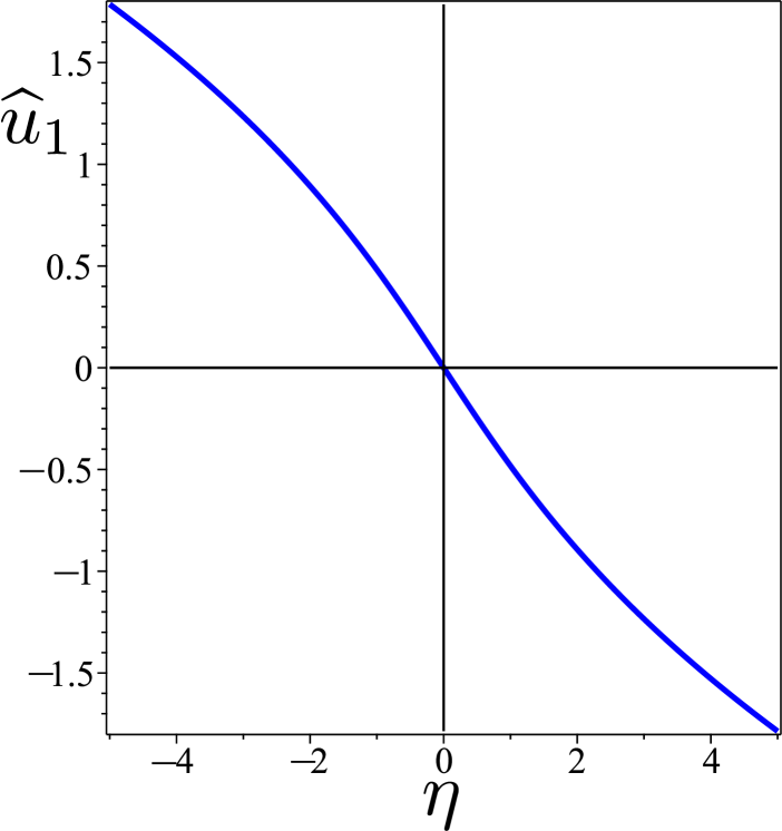
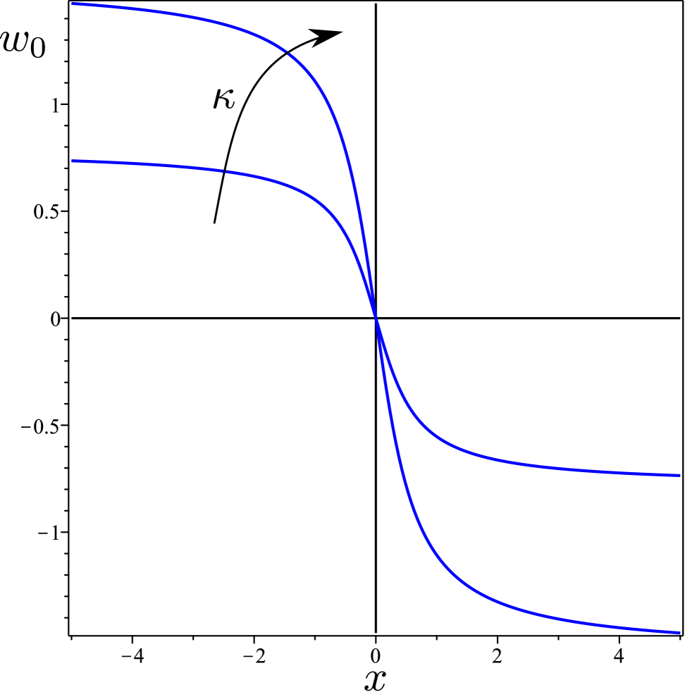
where is the maximal interval of classical existence. We need to express as a function of and for (21) to acquire the desired form; by setting , with no prejudice for the validity of (20), the combination of (19) and (13) yields the relation
| (22) |
By inverting (22), can be expressed in terms of the difference
| (23) |
as
| (24) |
The graph of is represented in Fig. 1(a).
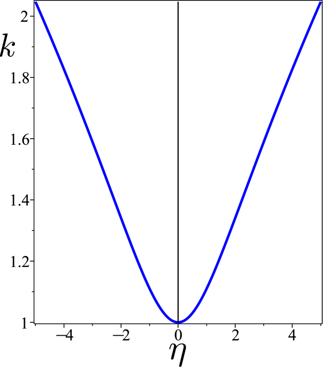
In (19), we can thus fomally replace the function with
| (25) |
finally arriving at
| , | (26a) | ||||
| , | (26b) | ||||
subject to initial conditions
| (27) |
The graph of the function in (25) is illustrated in Fig. 1(b).
Remark 2.
The characteristics of (26) are families of curves and , parametrized by , which, in the inviscid case, represent the trajectories along which the corresponding Riemann functions and remain constant. More precisely, the curve starting from a point at is the solution of the following differential problem
| (30) |
Similarly, the curve starting from a point at solves
| (31) |
Definition 1.
For brevity, we often say that and belong to the first and second families of characteristics, respectively. Since , we shall also say that is the forward characteristic, whereas is the backward characteristic.
Remark 3.
The reader should be advised though that this definition is not universally accepted: in equations (3.52) of [24], for example, the role of the two characteristics is interchanged.
Based on the definition of characteristics and , we introduce a concise notation for the derivatives along these curves of any smooth function .
Definition 2.
For any smooth function , we set
| (32) |
and call it the forward derivative of . Similarly, we set
| (33) |
and call it the backward derivative of .
As is apparent from (26), in the dissipative case the Riemann functions and in (19) fail to be constant along characteristics. Instead, they obey the following laws,
| (34) |
Remark 4.
Remark 5.
The system (34) governing the evolution of the Riemann functions along characteristics remains locally well-posed under the given initial conditions and assumptions. Indeed, since is bounded by assumption, the initial values of the Riemann functions, and , expressed in (27) in terms of , are bounded continuous functions with bounded continuous derivatives. Under these hypotheses, the general theory presented in [28] ensures that the strictly hyperbolic system (26) has a unique solution locally in time.
III.2 Boundedness of Riemann Functions
In the following, we assume that, for a given value of , the pair is the unique solution of the system (26) in , subject to the initial conditions in (27) with . Building on the framework recently proposed in [29, 30] for dissipative problems, we define
| (35) |
and rephrase the evolution laws in (34) as
| (36) |
Integrating both sides of (36) and taking into account the initial conditions in (27), we obtain that
| (37) |
In the dissipative case, and are no longer constant along the characteristics of (26), but they remain uniformly bounded over time, as we now proceed to show.
Lemma 1.
Let and . Then, for a solution of the system (26) of class over ,
| (38a) | ||||
| (38b) | ||||
The proof of Lemma 1 employs the strategy used in the proof of Lemma 7 in [29]; its adaptation to our context is deferred to Appendix A.
Remark 6.
Definition 3.
By the continuation principle (see, for example, [24, p. 100] for this particular incarnation), the estimates (39) imply the following dichotomy: for a given value of , either there is a critical time such that
| (40) |
or there is a global smooth solution of (19) for all . In the former case, which is the one we are interested in, a shock wave is formed in a finite time. In the latter case, we conventionally set .
III.3 Energy Dissipation and Mass Conservation
Here, we show that regular solutions of the system (15) in dissipate energy while preserving mass.111The latter is meant as a synonym for the total twist. We shall employ the following lemma, which asserts that the limits of the spatial derivative of the twist angle , as approaches , coincide with the limits of the derivatives of the initial datum .
Lemma 2.
Let be finite. Then, for a solution of the system (15), the following limits hold for every ,
| (42) |
Similarly, since for all , then
| (43) |
for every .
The proof of Lemma 2 can be found in Appendix A; it is an extension to our present context of a similar result proved in Lemma 8 of [29]. Building upon Lemma 2, we derive a dissipation law for the total energy associated with the system (15), which comprises a quadratic kinetic energy and a quartic potential energy.
Proposition 1.
Thus, the energy of the system decreases over time due to the damping term; the rate of dissipation is proportional to the integral of , which represents the kinetic energy of the system.
Proof.
Proposition 2.
IV Pre-Breakdown Properties
Here, we prepare the ground for the analysis of the formation of discontinuities in the derivatives of the Riemann functions that will be performed in the following section. Detailed proof of the following preparatory results are deferred to Appendix A.
IV.1 Evolution along characteristics
We first focus on the behavior of the spatial derivatives of the solutions and of (26) along the characteristic curves described by (30) and (31). This is meant to lay the foundation for the analysis of shock formation along characteristics. We are primarily interested in sufficient conditions for the breakdown of solutions.
Definition 4.
Let the pair be a solution of class of (26). We define the pair of weighted Riemann derivatives as
| (51a) | ||||
| (51b) | ||||
The following Proposition analyzes the behavior of along the characteristic curves and , respectively.
Proposition 3.
If the pair is a solution of class of (26), then the pair satisfies
| (52a) | ||||
| (52b) | ||||
where is the function defined by
| (53) |
Proof.
Using Definition 2, we obtain that
| (54) |
where all quantities are evaluated along the characteristic curve . By differentiating both sides of the first equation in (34) with respect to and using (54), we obtain that
| (55) |
Similarly, we have that
| (56) |
where all quantities are evaluated along the characteristic curve . From (22) and (21) we can also derive the equations
| (57) |
Then, by multiplying both sides of (55) and (56) by evaluated at and , respectively, and making use of (51) and (53), we obtain (52). ∎
Remark 8.
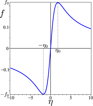
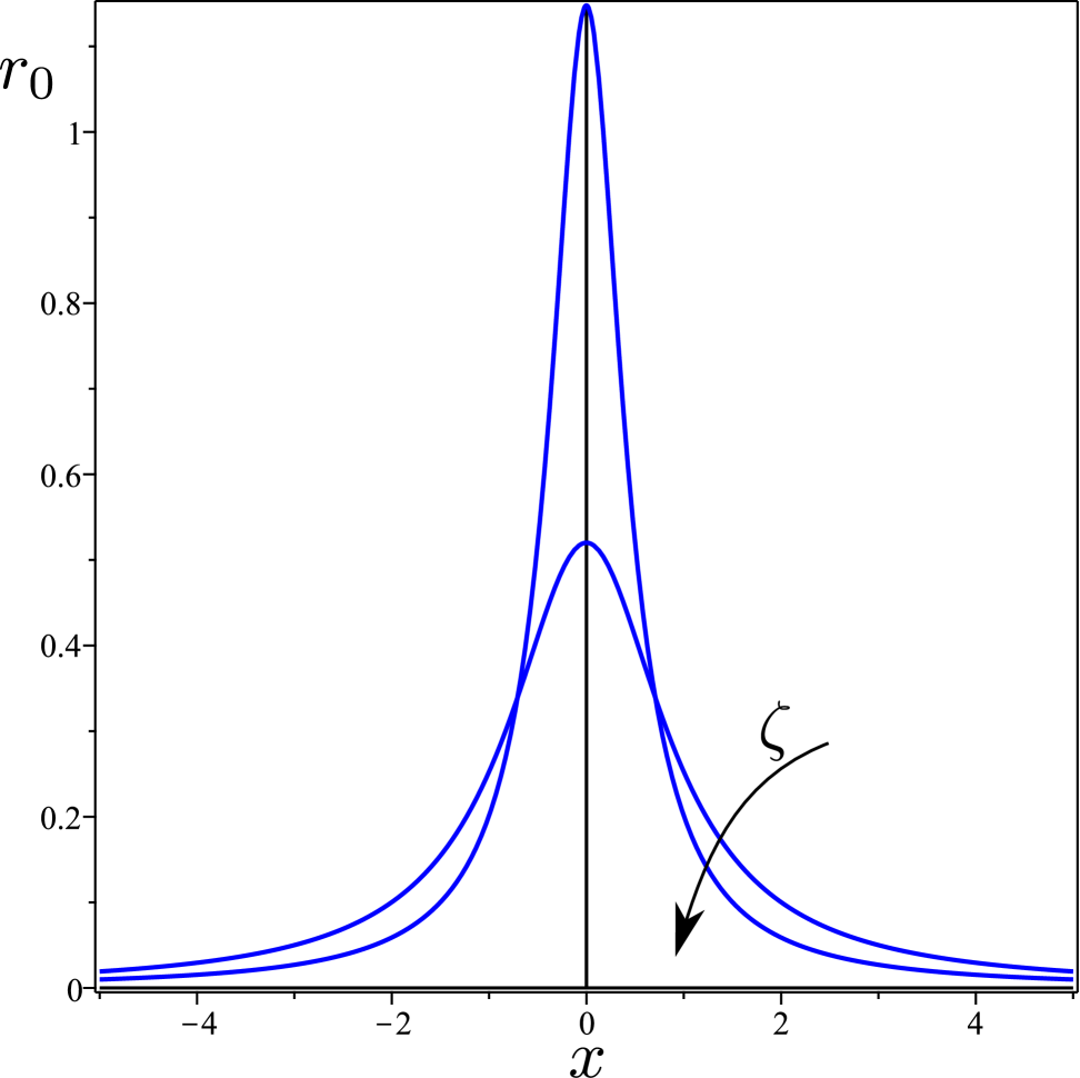
Since is defined implicitly by (25), it is better represented in parametric form. By differentiating both sides of (25), and using (13), (20), and (24), we easily arrive at
| (58) |
the former being simply (22) rewritten. It is clear from (58) that is an odd function of . It exhibits an isolated minimum at and an isolated maximum at , whose values are , respectively, corresponding to the values of the parameter in (58).
The graph of the function is illustrated in Fig. 2.
IV.2 Damped Shock Waves
A critical aspect of our analysis is to identify every point reached by a characteristic of one family as the end-point, at time , of a characteristic in the other family. This identification is formalized by the functions and defined as follows.
Definition 5.
Every point reached by a forward characteristic can be seen as the end-point at time of a backward characteristic originating at , where is formally defined by
| (59a) | |||
| Conversely, by exchanging the roles of forward and backward characteristics, the function is defined implicitly by | |||
| (59b) | |||
Instrumental to the analysis of the mappings and are the wave infinitesimal compression ratios, which can be defined as follows.
Definition 6.
For every characteristic curve, and , corresponding to a smooth solution of (26), the wave infinitesimal compression ratios, and , are defined by
| (60) |
Proposition 4.
If the pair is a local solution of class of the system (26) in , then the wave infinitesimal compression ratios and are given by
| (61a) | ||||
| (61b) | ||||
Remark 9.
As long as both and are of class , inequalities (61) remain valid, and vice versa, meaning that characteristics in the same family do not crash on one another.
Since both and are always positive for regular solutions, we can then derive the following properties for the mappings and . This result is proved in Appendix A
Proposition 5.
Remark 10.
It readily follows from (63) that and .
Definition 7.
For a given value of , we say that a shock wave is formed when either or in (51) diverges along one family of characteristics. Specifically, this requires either that there is and a finite time such that
| (64) |
or that there is and a finite time such that
| (65) |
By (51), this in turn implies that either diverges as or diverges as . Finally, according to (19) and (17), as a shock wave arises, the second derivatives of diverge, while its first derivatives develop a discontinuity.
Remark 11.
Remark 12.
Not to burden our presentation with too many case distinctions, we shall preferentially focus on the divergence of along forward characteristics. When both and diverge, the critical time is the least between and , for all admissible and for which these times exist.
In the following section, we shall derive estimates for and record without explicit proof the corresponding estimates for .
V Critical time estimates
By applying the method illustrated in the preceding section, we shall determine a range of values of for which singularities in the smooth solutions of problem (15) occur for a wide class of initial data . We shall provide an estimate for the critical time , which depends only on and (through ).
V.1 Auxiliary Lemmas
The following lemma asserts that along forward characteristic curves departing from values of where specific properties of the initial condition in (27) are satisfied, the function remains confined between two functions of time determined by .
Lemma 3.
Let and let the pair be a solution of class of the system (26) for with initial condition in (27). Assume that is bounded and has a finite limit as ,
| (66) |
If there exists at least one such that satisfies both
| (67) |
then, along the characteristic curve , is confined between two functions,
| (68) |
where
| (69) | ||||
| (70) |
Proof.
For the proof of this lemma, we focus on one of the alternatives contemplated in (67), that is,
| (71) |
The other alternative can be treated in exactly the same way. The proof employs a recursive argument to improve progressively lower and upper bounds on the function
| (72) |
By Proposition 5, the point , where is to be evaluated, is the end-point at time of the backward characteristic starting from . Hence, by (36),
| (73) |
This identity is instrumental to our recursive method.
Step .
We start by rewriting equation (V.1) as
| (74) |
where
| (75a) | ||||
| (75b) | ||||
By Lemma 1 and Remark 6, we have that
| (76) |
By using (76) in (74), we obtain the following upper and lower bounds for ,
| (77) |
where (35) has also been used. By (35), (77) provides a first estimate for upper and lower bounds on . To refine this estimate we proceed recursively. We know from (36) that along the characteristic curves and through the points and ,
| (78) |
from which it follows that
| (79) |
Step .
We apply equation (79) to the integrand in (74): and can be seen as end-points at time of the characteristic curves and , respectively, where both and range between and for . Thus, we can write
| (80) |
By use of (V.1) in (74), we arrive at
| (81) |
where
| (82a) | ||||
| (82b) | ||||
We now estimate for . By (71), both and range between and for , and since , by (82a),
| (83) |
Moreover, by applying Lemma 1 and Remark 6 to (82b), we obtain that
| (84) |
By inserting (84) into (81) and using again (35), we find that
| (85) |
and
| (86) |
Step .
We now apply formula (79) to in (82b): and can be seen as the end-points at time of the characteristic curves and , with and as . Therefore, for in , both and lie within the interval . Then, in (81) we can write
| (87) |
where
| (88a) | ||||
| (88b) | ||||
and (81) becomes
| (89) |
As above, by (71), every in (V.1) ranges between and , while, by Lemma 1 and Remark 6, is bounded by , and so
| (90) |
and
| (91) |
where use of (35) has again been made.
The steps illustrated above outline already a clear pattern. By repeated applications of this method, we easily reach any higher level of recursion.
Step .
Thus, for , we arrive at
| (92a) | |||
| and | |||
| (92b) | |||
Taking in (92) the limit as delivers
| (93) |
whence the inequalities in (68) follow easily, also by use of (72) and (75a). ∎
Remark 13.
To determine the sign of as elapses, an additional hypothesis on the sign of is required in addition to conditions (67).
Lemma 4.
Proof.
Remark 14.
In the following lemma, we state a property similar to that found in Remark 14 for the function .
Lemma 5.
Let the pair be a solution of class of the system (26) for with initial condition such that as in (27). Assume that is bounded and has a finite limit as , as in (66). Assume further that there exists at least one such that (67), and (95) hold. Then, for every such that
| (99) |
we have that
| (100) |
where is defined as in (51b).
Proof.
Here, we focus on the specific case of (67) and (95) embodied by
| (101) |
The complementary case arising from assuming that is analogous and can be treated similarly. By (30), (32), and (57), we can rewrite the definition of in (51b) as
| (102) |
where is such that
| (103) |
By integrating by parts in (102), we obtain that
| (104) |
and to prove (100) it suffices to show that the right-hand side of (104) is positive. Under hypothesis (101), by Lemma 4 and Remark 14, the function is always positive and bounded below by the positive and strictly decreasing function in (69). Accordingly, by (103) is a decreasing function of for every , and so
| (105) |
Moreover, since
| (106) |
is concave for every . Thus, the right-hand side of (104) can be estimated as
| (107a) | ||||
| (107b) | ||||
| (107c) | ||||
where inequality (107b) follows from the concavity of and use is made in (107c) of (69), (70), and (103). By (101), for , and so (107c)implies (100). ∎
Remark 15.
The function is hard to find explicitly, but its bounds in (63) provide explicit estimates for :
| (108) |
where
| (109) |
with defined in (41). Since the function is monotonically increasing with time, the function retains the same properties as outlined in Lemma 4 and Remark 14: thus, under conditions (67) and (95),
| (110) |
Moreover, from (108) we obtain that
| (111) |
and so the conclusion of Lemma 5 also applies under the following condition
| (112) |
which strengthens (99) and will replace it in our development below.
V.2 Main Result
We now provide an estimate for the critical time at which a singularity occurs in a forward characteristics under the assumptions (67) and (95). This estimate will be acceptable only if it satisfies (112).
Theorem 1.
Consider the global Cauchy problem (26) with initial condition such that as in (27). Suppose that for a given there exists at least one such that satisfies conditions (67) and (95). Then the solution to (26) is predicted to develop a singularity along the characteristic curve in a finite time , provided that there exists a solution to the following equation for ,
| (113) |
where is defined as
| (114) |
with as in (109), and provided that at inequality (112) is satisfied.
Proof.
As above, for the proof of this theorem, we focus again on the specific case where conditions (67) and (95) are specialized as in (101). We first consider the ordinary differential equation in (52a). By integrating in time, can be written along the forward characteristic as
| (115) |
Here, by (51a),
| (116) |
By Lemma 5, for every such that (112) holds,
| (117) |
and so
| (118) |
Moreover, according to Lemma 4, under conditions (101) is positive for every . Since for all , in (118) is also positive for every , and so
| (119) |
from which we arrive at
| (120) |
Let now satisfy
| (121) |
so that, by (120),
| (122) |
By applying to (122) the comparison theorem stated in Appendix A, by (119), we find that
| (123) |
where is the solution of (121),
| (124) |
By (116), diverges to in a finite time if
| (125) |
and, by (123) and (51a), so also does along the characteristic curve .
Remark 16.
The proof of Theorem 1 essentially relies on the existence for all times of solutions for the following Riccati equation,
| (129) |
which reduces to (52a) once we set
| (130a) | ||||
| (130b) | ||||
| (130c) | ||||
Were we able to determine the sign of or verify whether , for some differentiable and non-decreasing function , we could either guarantee solvability of (129) for all times [31], or blow-up in a finite time [32, 33, 34]. However, by (57), controlling the sign of amounts to control the sign of the derivative along forward characteristics, which is a far more demanding task than the bounds delivered by (68) can accomplish. In our study, the control of the sign of is replaced by the estimate in (118).
Remark 17.
A parallel argument applied to backward characteristics proves that if has a finite limit as ,
| (131) |
and if there exists at least one such that satisfies the conditions
| (132a) | |||
| (132b) | |||
then the solution to (26) will develop a singularity along the characteristic curve in a finite time , provided that
-
1.
there exists a solution to the following equation for ,
(133) where is defined as
(134) and
(135) -
2.
at the following inequality is satisfied,
(136)
Remark 18.
We now consider the inviscid limit of Theorem 1. For , (94) applies and since, by (63), for every , (62) implies that under conditions (67) is monotonic and does not change sign for all . Thus, the asymptotic limit approached as has the same sign as . This implies that
| (137) |
so that
| (138) |
and (113) becomes
| (139) |
which is precisely the estimate achieved in Corollary 1 of [17]. We finally also note that in the inviscid case, inequality (112) need not be satisfied.
Theorem 1 estimates , for given and . An estimate for the critical time follows from minimizing over all ’s for which a singularity occurs, as summarized in the following proposition.
Proposition 6.
VI Application
As an illustrative example, we consider an initial profile for the twist angle that exhibits a strong concentration of distortion around , which fades away at infinity without ever vanishing. Thus, by (13), the more distorted core is expected to propagate faster than the distant tails, possibly overtaking them: intuitively, this should prompt the creation of a singularity in a finite time. We shall see here how such an intuitive prediction is indeed confirmed by the estimate (141).
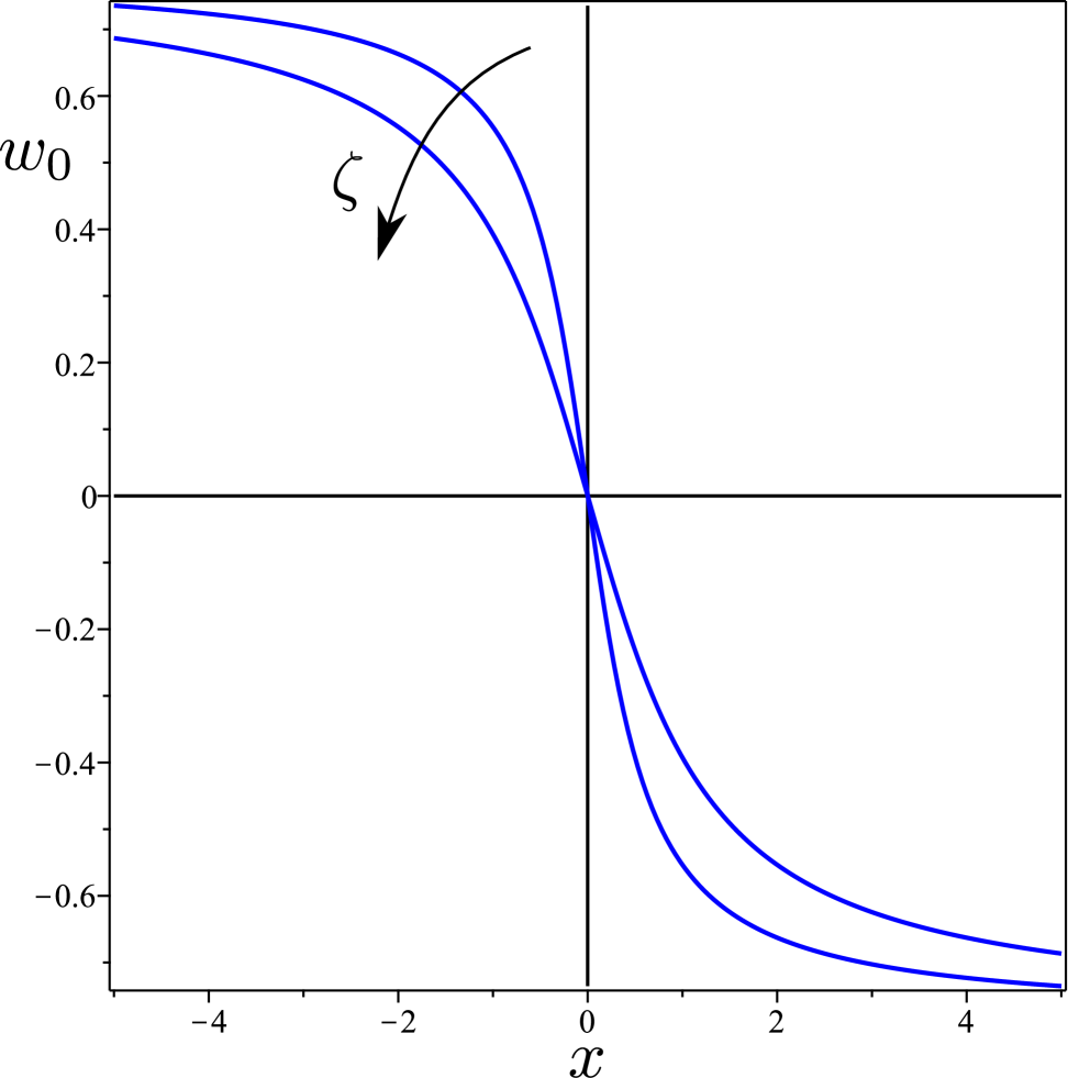
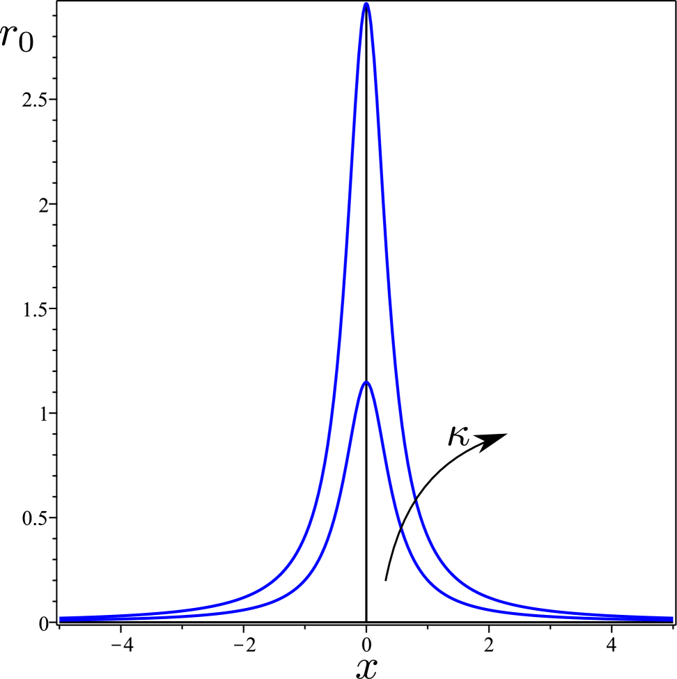
We consider the following initial twist profile
| (142) |
where and are positive parameters. This is a kink representing a smooth transition of the twist angle between two asymptotic values depending on over an effective width depending on . Fig. 3 illustrates the graphs of the initial profile in (142) for different values of and : either increasing or decreasing makes the initial profile less distorted (whereas either decreasing or increasing makes the initial profile more distorted).
| (143) |
The graph of is illustrated in Fig. 4 for different values of and . Since is an even function, by Theorem 1, we need only consider forward characteristics: if a singularity arises along a forward characteristic originating at , a singularity will also occur at the same critical time along the (symmetric) backward characteristic originating at .
Here, and conditions (67) and (95) are satisfied for every . Thus, by Theorem 1 a singularity can occur in a finite time , provided that there is a root of (113) for that obeys (112).
To compute the infimum of for any given , we find it convenient to compute first the pre-critical time defined as
| (144) |
where
| (145) |
and then use (112) as a selection rule: we set , if (112) is valid for and ;222In most practical cases, the infimum is attained and (112) is computed for . otherwise, we set .
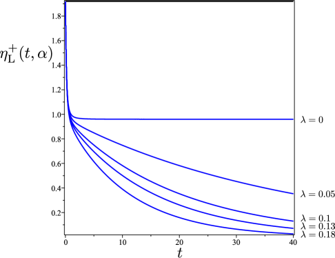
We start by studying the function in (109); its graph against is represented in Fig. 5 for different values of . As observed in Lemma 4 and Remark 14, its behavior reproduces for that of for : it is strictly decreasing and stays positive as time elapses.
Blue lines in Fig. 6 show how the pre-critical time depends on for fixed and . In accord with physical intuition, is a monotonically increasing function of : as increases, the wave undergoes a greater damping, resulting in a stronger progressive attenuation over time and a corresponding delay in forming shocks. Furthermore, for given , decreases as decreases and increases as increases: a decrease in or an increase in results indeed in a wider or lower initial profile, suggesting that the kink’s core propagates more slowly, thus delaying the occurrence of shocks. Figure 6 also brings to effect the selection rule (112); the acceptable range of for the validity of our theory is determined graphically as the maximum interval over which the red line is above the blue one. The cases shown in Fig. 6 seem to indicate that the acceptable range of increases when either the amplitude of the kink increases or the width decreases.
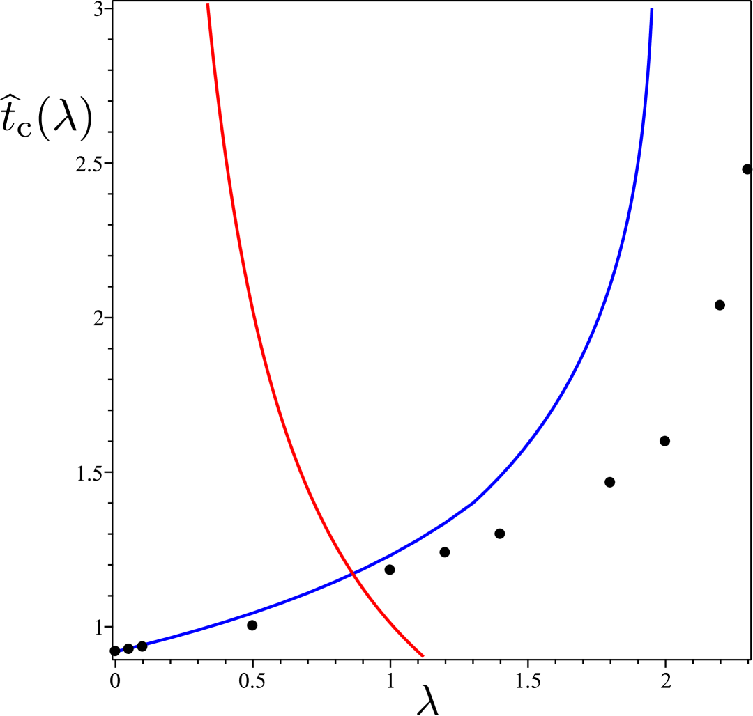
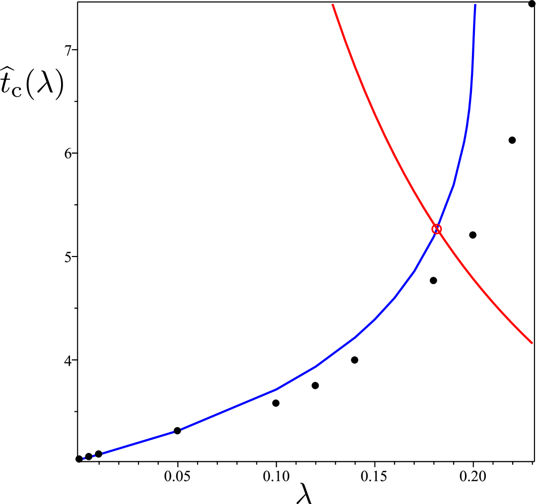
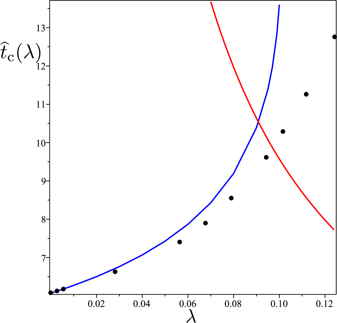
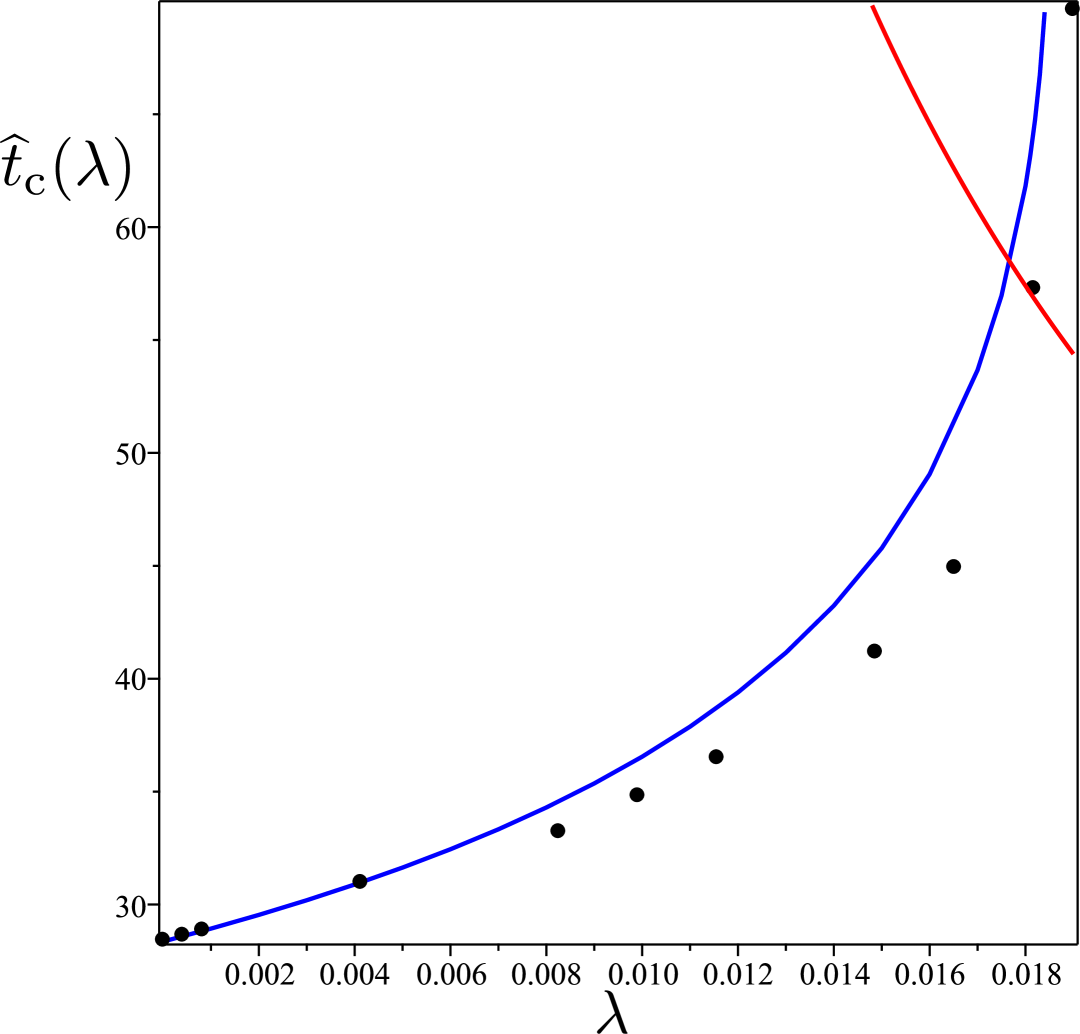
Numerical solutions of the Cauchy problem (15) closely corroborate our theoretical predictions. Black dots in Fig. 6 represent critical times computed numerically for different values of , with fixed and . Within the range of validity of our theory, these numerical values are in close agreement with the estimated values of the pre-critical times .
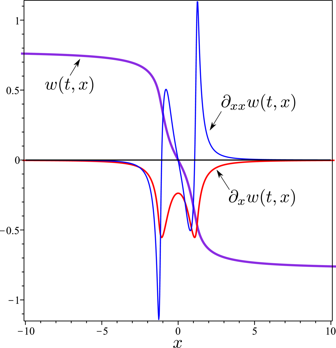
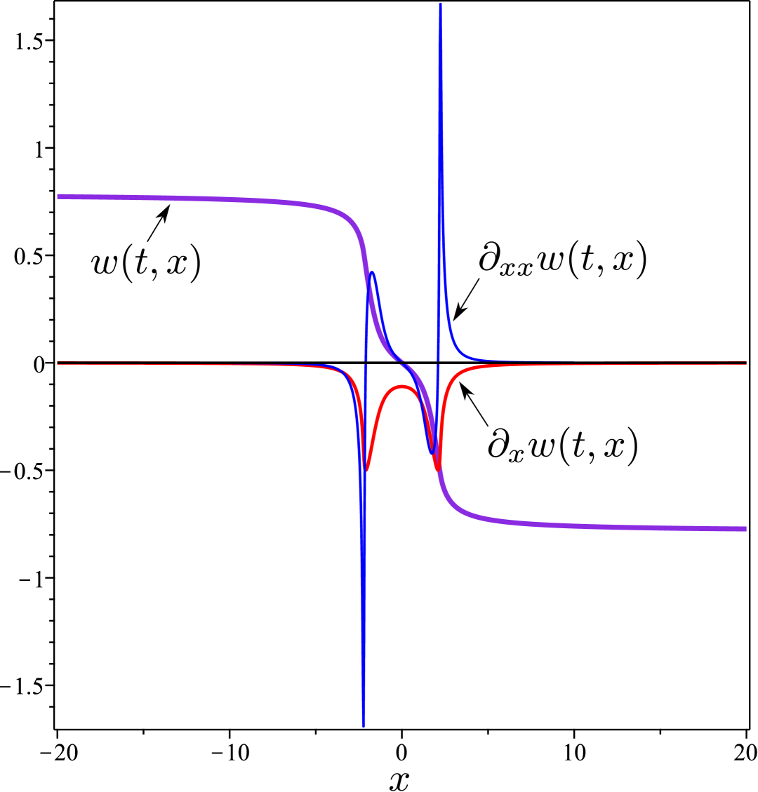
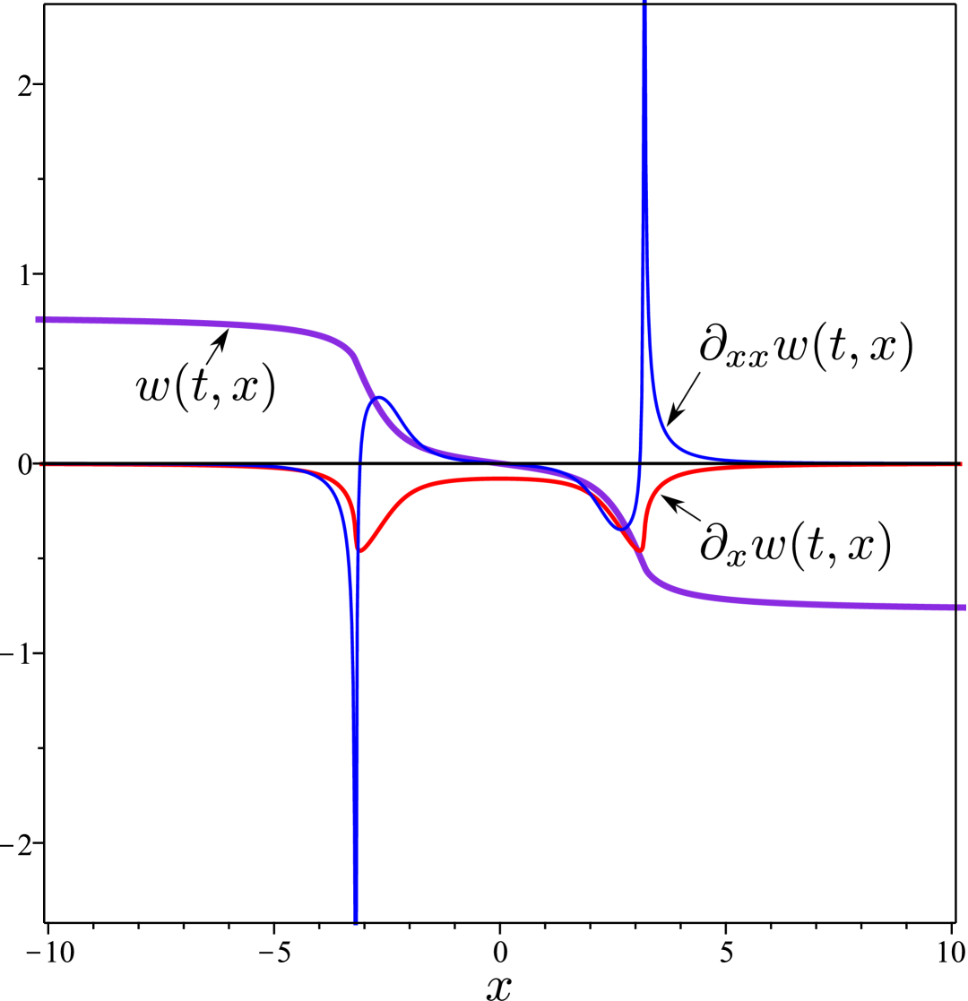
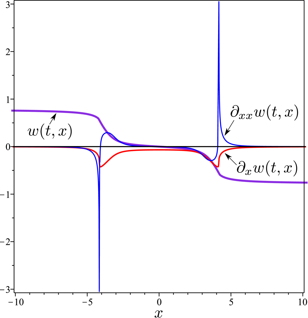
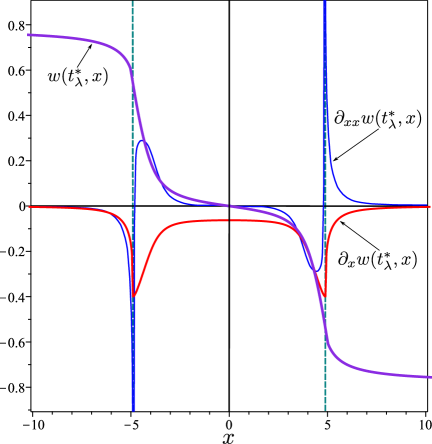
We paid special attention to the case where in (142) and ; for these specific values of and , is the upper acceptable limit for the validity of our theory. The initial profile generates two symmetric waves propagating in opposite directions. We computed the conserved quantity and the decaying quantity introduced in Propositions 2 and 1, respectively, and used them to monitor the accuracy of our numerical solutions. Our calculations indicate the existence of a critical time, estimated as , at which the solution exhibits a singularity. Fig. 7 illustrates a typical numerical solution and its spatial derivatives and for a sequence of times in the interval . A snapshot at is shown in Fig. 8. The observed behavior is in good agreement with our theory: a shock is formed in a finite time, at which becomes discontinuous, and second derivatives diverge.
The critical time identified numerically agrees with our theoretical upper estimate ; the infimum in (141) is correspondingly attained for .
VII Conclusions
The relaxation dynamics of liquid crystals involves only the motion of the director which represents the average molecular orientation; no hydrodynamic flow is entrained. The director motion is hampered by rotational viscosity and, in ordinary nematic liquid crystals, it drives the fluid smoothly towards equilibrium.
Such a state of affairs, common to many dissipative systems, does not apply to chromonic liquid crystals. They are as dissipative as ordinary nematic liquid crystals, but their elasticity is better represented by a free-energy density quartic in the director gradient, instead of quadratic, as in the celebrated Oseen-Frank formula for ordinary nematics. This peculiar aspect of chromonics affects deeply the propagation of twist waves. It was proved in [17] that in the inviscid limit, where all sources of dissipation are neglected, a twist wave generally develops a singularity, giving rise to a shock wave in finite time.
The present study, which is the ideal sequel of [17], was concerned with the possible regularizing effect of dissipation. We asked whether a finite degree of dissipation could systematically prevent singularities from arising, thus leading smoothly the system to stillness.
We answered this question for the negative: We provided a criterion for the choice of the initial data that guarantees the formation of a shock wave and estimated the critical time for its manifestation. This criterion was also subject to a numerical validation; for a class of initial director profiles our estimate for the critical time proved to be accurate, more so for small values of the dimensionless parameter that weights dissipation against elasticity.
This is the main achievement of our paper, but it came at a price. A selection rule had to be enforced on the time interval where our analytical method is applicable. Such a rule effectively reduces the range of acceptable values of in a manner influenced by the initial director profile.
Although, we provided a tool to probe the range of confidence of our method, this limitation can hardly be ignored. It is likely to stem from the role played here by the Riemann functions: they are no longer invariant in the dissipative setting, but they are still the main players in our analysis. We might have pushed this method to the extreme and paid a price in generality.
We have established that dissipation does nor prevent shocks to develop in chromonic twist waves, but an important question remains unanswered: is there a critical value of (possibly affected by the initial director profile) above which singularities are banned and twist waves fade away uneventfully? The answer to this might come from an approach different from the one taken here.
Acknowledgements.
Both authors are members of GNFM, a branch of INdAM, the Italian Institute for Advanced Mathematics. For the most part, this work was performed while S.P. was holding a Postdoctoral Fellowship with the Department of Mathematics of the University of Pavia. Their kind hospitality during later times, while this paper was completed, is gratefully acknowledged.Appendix A Auxiliary Results
In this Appendix, we collect a number of auxiliary results needed in the main text, including the proofs of Lemmata 1 and 2, and that of Propositions 4 and 5.
We start by stating a comparison theorem (see Theorem 1.3 of [35]).
Theorem 2 (Comparison Theorem).
If is a function locally Lipschitz continuous in and uniformly continuous in , and if and are two differentiable functions such that
| (146) |
then
| (147) |
To apply this theorem to (122), it suffices to take
| (148) |
where . The function in (148) is clearly locally Lipschitz continuous in and uniformly continuous in , given the regularity of the solution and its boundedness (by Lemma 1).
Proof of Lemma 1.
We only prove (38a). On the characteristic curves and with and selected so that these curves pass through the points and , respectively, by (36), we obtain that
| (149) |
By the definition of in Lemma 1, this equation is equivalent to
| (150) |
and by taking the -norm of both sides of (150) with , we arrive at
| (151) |
By the classical Grönwall’s inequality, it then follows that
| (152) |
which implies inequality (38a) in the main text. Inequality (38b) can be proved in precisely the same way. ∎
Proof of Lemma 2.
Since can be expressed through (17) and (24) in terms of ,
| (153) |
we prove Lemma 2 by studying the behaviour of for . We set
| (154a) | ||||
| (154b) | ||||
and we consider the characteristic curves and with and selected so that these curves meet at a given point ; as long as the solution remains regular, they are uniquely identified (see Proposition 5 in the main text). Then, by (36), we can express as
| (155) |
Since for any given , , by the arbitrariness of , it follows from (155) that
| (156) |
where the last inequality is obtained through the Lebesgue Convergence Theorem, since the function is bounded for every and for every by (38b). By the classical Grönwall’s inequality, we then obtain that
| (157) |
In a similar way, we also prove that
| (158) |
Since by definition, (157) and (158) imply that
| (159) |
Proof of Proposition 4.
By differentiating both sides of the first equation in (30) with respect to , we find that
| (161) |
Letting
| (162) |
where also (25) has been used, by (32) we arrive at
| (163) |
Then, (161) reduces to
| (164) |
which can be set in the form
| (165) |
where, also by (51a),
| (166) |
The solution of (165) subject to the initial condition is the following,
| (167) |
Since, by (166) and (27), , (167) delivers equation (61a) in the main text.
Equation (61b) is obtained in a similar way. ∎
Proof of Proposition 5.
The existence of the unique solution is a consequence of the fact that the Cauchy problem
| (168) |
has a unique solution for every . We set and , where is solution of (31). Thus, represents the point from which the backward characteristic starts. By (31), we conclude that for every and . By differentiating both sides of equation (59a) with respect to , and using (30) and (31), we obtain (62).
References
- Shiyanovskii et al. [2005] S. V. Shiyanovskii, T. Schneider, I. I. Smalyukh, T. Ishikawa, G. D. Niehaus, K. J. Doane, C. J. Woolverton, and O. D. Lavrentovich, Real-time microbe detection based on director distortions around growing immune complexes in lyotropic chromonic liquid crystals, Phys. Rev. E 71, 020702 (2005).
- Mushenheim et al. [2014a] P. C. Mushenheim, R. R. Trivedi, H. H. Tuson, D. B. Weibel, and N. L. Abbott, Dynamic self-assembly of motile bacteria in liquid crystals, Soft Matter 10, 88 (2014a).
- Mushenheim et al. [2014b] P. C. Mushenheim, R. R. Trivedi, D. Weibel, and N. Abbott, Using liquid crystals to reveal how mechanical anisotropy changes interfacial behaviors of motile bacteria, Biophys. J. 107, 255 (2014b).
- Zhou et al. [2014] S. Zhou, A. Sokolov, O. D. Lavrentovich, and I. S. Aranson, Living liquid crystals, Proc. Natl. Acad. Sci. USA 111, 1265 (2014).
- Lydon [1998a] J. Lydon, Chromonic liquid crystal phases, Curr. Opin. Colloid Interface Sci. 3, 458 (1998a).
- Lydon [1998b] J. Lydon, Chromonics, in Handbook of Liquid Crystals: Low Molecular Weight Liquid Crystals II, edited by D. Demus, J. Goodby, G. W. Gray, H.-W. Spiess, and V. Vill (John Wiley & Sons, Weinheim, Germany, 1998) Chap. XVIII, pp. 981–1007.
- Lydon [2010] J. Lydon, Chromonic review, J. Mater. Chem. 20, 10071 (2010).
- Lydon [2011] J. Lydon, Chromonic liquid crystalline phases, Liq. Cryst. 38, 1663 (2011).
- Dierking and Martins Figueiredo Neto [2020] I. Dierking and A. Martins Figueiredo Neto, Novel trends in lyotropic liquid crystals, Crystals 10, 604 (2020).
- Oseen [1933] C. W. Oseen, The theory of liquid crystals, Trans. Faraday Soc. 29, 883 (1933).
- Frank [1958] F. C. Frank, On the theory of liquid crystals, Discuss. Faraday Soc. 25, 19 (1958).
- Paparini and Virga [2022] S. Paparini and E. G. Virga, Paradoxes for chromonic liquid crystal droplets, Phys. Rev. E 106, 044703 (2022).
- Paparini and Virga [2024a] S. Paparini and E. G. Virga, An elastic quartic twist theory for chromonic liquid crystals, J. Elast. 155, 469 (2024a).
- Paparini and Virga [2023] S. Paparini and E. G. Virga, Spiralling defect cores in chromonic hedgehogs, Liq. Cryst. 50, 1498 (2023).
- Ciuchi et al. [2024] F. Ciuchi, M. P. De Santo, S. Paparini, L. Spina, and E. G. Virga, Inversion ring in chromonic twisted hedgehogs: theory and experiment, Liq. Cryst. 51, 2381 (2024).
- Paparini and Virga [2024b] S. Paparini and E. G. Virga, What a twist cell experiment tells about a quartic twist theory for chromonics, Liq. Cryst. 51, 993 (2024b).
- Paparini and Virga [2025] S. Paparini and E. G. Virga, Singular twist waves in chromonic liquid crystals, Wave Motion 134, 103486 (2025).
- Manfrin [2000] R. Manfrin, A note on the formation of singularities for quasi-linear hyperbolic systems, SIAM J. Math. Anal. 32, 261 (2000).
- Selinger [2018] J. V. Selinger, Interpretation of saddle-splay and the Oseen-Frank free energy in liquid crystals, Liq. Cryst. Rev. 6, 129 (2018).
- Selinger [2022] J. V. Selinger, Director deformations, geometric frustration, and modulated phases in liquid crystals, Ann. Rev. Condens. Matter Phys. 13, 49 (2022).
- Pedrini and Virga [2020] A. Pedrini and E. G. Virga, Liquid crystal distortions revealed by an octupolar tensor, Phys. Rev. E 101, 012703 (2020).
- Ericksen [1991] J. L. Ericksen, Liquid crystals with variable degree of orientation, Arch. Rational Mech. Anal. 113, 97 (1991).
- Ericksen [1968] J. L. Ericksen, Twist waves in liquid crystals, Q. J. Mech. Appl. Math. 21, 463 (1968).
- Majda [1984] A. Majda, Compressible Fluid Flow and Systems of Conservation Laws in Several Space Variables, Applied Mathematical Sciences, Vol. 53 (Springer-Verlag, New York, 1984).
- MacCamy and Mizel [1967] R. C. MacCamy and V. J. Mizel, Existence and nonexistence in the large of solutions of quasilinear wave equations, Arch. Rational Mech. Anal. 25, 299 (1967).
- Chang [1977] P. H. Chang, On the existence of shock curves of quasilinear wave equations, Indiana Univ. Math. J. 26, 605 (1977).
- Klainerman and Majda [1980] S. Klainerman and A. Majda, Formation of singularities for wave equations including the nonlinear vibrating string, Comm. Pure Appl. Math. 33, 241 (1980).
- Douglis [1952] A. Douglis, Some existence theorems for hyperbolic systems of partial differential equations in two independent variables, Comm. Pure Appl. Math. 5, 119 (1952).
- Sugiyama [2018] Y. Sugiyama, Singularity formation for the 1D compressible Euler equations with variable damping coefficient, Nonlinear Anal. 170, 70 (2018).
- [30] Y. Sui and H. Yu, Vacuum and singularity formation problem for compressible Euler equations with general pressure law and time-dependent damping, Nonlinear Anal. Real World Appl. 65, https://doi.org/10.1016/j.nonrwa.2021.103472.
- Grigoryan [2015] G. A. Grigoryan, Global solvability of scalar Riccati equations, Russ. Math. 59, 31 (2015).
- Wei [2021] L. Wei, New wave-breaking criteria for the Fornberg-Whitham equation, Differ. Equ. 280, 571 (2021).
- Baris et al. [2006] J. Baris, P. Baris, and B. Ruchlewicz, On blow-up solutions of nonautonomous quadratic differential systems, Differ. Equ. 42, 320 (2006).
- Dou and Zhao [2021] C. Dou and Z. Zhao, Analytical solution to 1D compressible Navier-Stokes equations, J. Funct. Spaces 2021, 6339203 (2021).
- Teschl [2012] G. Teschl, Ordinary Differential Equations and Dynamical Systems, Graduate Studies in Mathematics, Vol. 140 (American Mathematical Society, Providence, 2012) available from https://www.mat.univie.ac.at/~gerald/ftp/book-ode/ode.pdf.