Dynamical Low-Rank Compression of Neural Networks with Robustness under Adversarial Attacks

Abstract

Deployment of neural networks on resource-constrained devices demands models that are both compact and robust to adversarial inputs. However, compression and adversarial robustness often conflict. In this work, we introduce a dynamical low-rank training scheme enhanced with a novel spectral regularizer that controls the condition number of the low-rank core in each layer. This approach mitigates the sensitivity of compressed models to adversarial perturbations without sacrificing clean accuracy. The method is model- and data-agnostic, computationally efficient, and supports rank adaptivity to automatically compress the network at hand. Extensive experiments across standard architectures, datasets, and adversarial attacks show the regularized networks can achieve over 94% compression while recovering or improving adversarial accuracy relative to uncompressed baselines.

1 Introduction

Deep neural networks have achieved state-of-the-art performance across a wide range of tasks in computer vision and data processing. However, their success comes at the cost of substantial computational and memory demands which hinder deployment in resource-constrained environments. While significant progress has been made in scaling up models through data centers and specialized hardware, a complementary and equally important challenge lies in the opposite direction: deploying accurate and robust models on low-power platforms such as unmanned aerial vehicles (UAVs) or surveillance sensors. These platforms often operate in remote locations with limited power and compute resources, and are expected to function autonomously over extended periods without human intervention.

This setting introduces three interdependent challenges:

• Compression: Models must operate under strict memory, compute, and energy budgets.

• Accuracy: Despite being compressed, models must maintain high performance to support critical decision-making.

• Robustness: Inputs may be corrupted by noise or adversarial perturbations, requiring models to be resilient under distributional shifts.

Recent work has shown that these three objectives are inherently at odds. Compression via low-rank steffen2022low or sparsity techniques guo2016dynamic often leads to reduced accuracy. Techniques to improve adversarial robustness—such as data augmentation lee2023generativeadversarialtrainerdefense or regularization-based defenses zhang2019theoreticallyprincipledtradeoffrobustness —frequently degrade clean accuracy. Moreover, it has been observed that compressed networks can exhibit increased sensitivity to adversarial attacks savostianova2023robustlowranktrainingapproximate . Finally, many methods to increase adversarial robustness of the model impose additional computational burdens during training 10302664 ; 9442932 or inference pmlr-v70-cisse17a ; hein2017formal ; liu2019advbnnimprovedadversarialdefense , further complicating deployment on constrained hardware.

Our Contribution. We summarize our main contributions as follows:

• Low-rank compression framework. We introduce a novel regularizer and training framework that yields low-rank compressed neural networks, achieving a more than $10\times$ reduction in both memory footprint and compute cost, while maintaining clean accuracy and adversarial robustness on par with full-rank baselines.

• Theoretical guarantees. We analyze the proposed regularizer and derive an explicit bound on the condition number $\kappa$ of each regularized layer. The bound gives further confidence that the regularizer improves adversarial performance.

• Preservation of performance. We prove analytically—and verify empirically—that our regularizer neither degrades training performance nor reduces clean validation accuracy across a variety of network architectures.

• Extensive empirical validation. We conduct comprehensive experiments on multiple architectures and datasets, demonstrating the effectiveness, robustness, and broad applicability of our method.

Beyond these core contributions, our approach is model- and data-agnostic, can be integrated seamlessly with existing adversarial defenses, and never requires assembling full-rank weight matrices – the last point guaranteeing a low memory footprint during training and inference. Moreover, by connecting to dynamical low-rank integration schemes and enabling convergence analysis via gradient flow, we offer new theoretical and algorithmic insights. Finally, the use of interpretable spectral metrics enhances the trustworthiness and analyzability of the compressed models.

2 Related work

Low-rank compression is a prominent approach for reducing the memory and computational cost of deep networks by constraining weights to lie in low-rank subspaces. Early methods used post-hoc matrix denton2014exploiting and tensor decompositions (lebedev2015speeding, ), while more recent approaches integrate low-rank constraints during training for improved efficiency and generalization.

Dynamical Low-Rank Training (DLRT) steffen2022low constrains network weights to evolve on a low-rank manifold throughout training, allowing substantial reductions in memory and FLOPs without requiring full-rank weight storage. The method has been extended to tensor-valued neural network layers zangrando2023rank , and federated learning schotthöfer2024federateddynamicallowranktraining . Pufferfish (wang2021pufferfish, ) restricts parameter updates to random low-dimensional subspaces, while intrinsic dimension methods (aghajanyan2020intrinsic, ) argue that many tasks can be learned in such subspaces. GaLore (zhao2024galore, ) reduces memory cost by projecting gradients onto low-rank subspaces.

In contrast, low-rank fine-tuning methods like LoRA (hu2021lora, ) inject trainable low-rank updates into a frozen pre-trained model, enabling efficient adaptation with few parameters. Extensions such as GeoLoRA schotthöfer2024geolorageometricintegrationparameter , AdaLoRA (zhang2023adalora, ), DyLoRA (valipour2023dylora, ), and DoRA (Mao2024DoRAEP, ) incorporate rank adaptation or structured updates, improving performance over static rank baselines. However, these fine-tuning methods do not reduce the cost of the full training and inference, thus are not applicable to address the need of promoting computational efficiency.

Improving adversarial robustness with orthogonal layers has been a recently studied topic in the literature anil2019sorting ; bansal2018can ; xie2017all ; cisse17_parseval ; savostianova2023robustlowranktrainingapproximate . Many of these methods can be classified as either a soft approach, where orthogonality is imposed weakly via a regularizer, or a hard approach where orthogonality is explicitly enforced in training.

Examples of soft approaches include the soft orthogonal (SO) regularizer xie2017all , double soft orthogonal regularizer bansal2018can , mutual coherance regularizer bansal2018can , and spectral normalization miyato2018spectral . These regularization-based approaches have several advantages; namely, they are more flexible to many problems/architectures and are amenable to transfer learning scenarios (since pertained models are admissible in the optimization space). However, influencing the spectrum weakly via regularization cannot enforce rigorous and explicit bounds on the spectrum.

Many hard approaches strongly enforce orthogonality/well-conditioned constraints by training on a chosen manifold using Riemannian optimization methods li2020efficientriemannianoptimizationstiefel ; Projection_like_Retractions ; savostianova2023robustlowranktrainingapproximate . A hard approach built for low-rank training is given in savostianova2023robustlowranktrainingapproximate ; this method clamps the extremes of the spectrum to improve the condition number during the coefficient update. The clamping gives a hard estimate on the range of the spectrum which enables a direct integration of the low-rank equations of motion with standard learning rates. However, this method requires a careful selection of the rank $r$, which is viewed as a hyperparameter in savostianova2023robustlowranktrainingapproximate . If $r$ is chosen incorrectly, the clamping of the spectrum, a hard-thresholding technique, acts as a strong regularizer which could affect the validation metrics of the network.

Our method falls neatly into a soft approach and our proposed regularizer can be seen as an extension of the soft orthogonality (SO) regularizer xie2017all to well-conditioned matrices in the low-rank setting. As noted in bansal2018can , the SO regularizer only works well when the input matrix is of size $m\times n$ where $m\leq n$. However, in our case we avoid this issue since the low-rank coefficient matrix $S$ is always square; an extension to convolutional layers is discussed in (4.1). In the context of low-rank training, the soft approach enables rank-adaptivity of the method.

3 Controlling the adversarial robustness of a neural network through the singular spectrum of its layers

We consider a neural network $f$ as a concatenation of $L$ layers $z^{\ell+1}=\sigma^{\ell}(W^{\ell}z^{\ell})$ with matrix valued parameters $W^{\ell}\in\mathbb{R}^{n\times n}$, layer input $z^{\ell}\in\mathbb{R}^{b\times n}$ and element-wise nonlinear activation $\sigma^{\ell}$. We do not consider biases, but a model with biases can always be formulated without them by folding them into the weights and creating a dimension that is always one. The data $X$ constitutes the input to the first layer, i.e. $z^{0}=X$. We assume that the layer activations $\sigma^{\ell}$ are Lipschitz continuous, which is the case for all popular activations savostianova2023robustlowranktrainingapproximate . The network is trained on a loss function $\mathcal{L}$ which we assume to be locally bounded and Lipschitz continuous gradient.

Low-rank Compression: The compression the network for training and inference is typically facilitated by approximating the layer weight matrices by a low-rank factorization $W^{\ell}=U^{\ell}S^{\ell}V^{\ell,\top}$ with $U^{\ell},V^{\ell}\in\mathbb{R}^{n\times r}$ and $S^{\ell}\in\mathbb{R}^{r\times r}$, where $r$ is the rank of the factorization. In this work, we generally assume that $U^{\ell},V^{\ell}$ are orthonormal matrices at all times during training and inference. This assumption deviates from standard low-rank training approaches hu2021lora , however recent literature provides methods that are able to fulfill this assumption approximately zhang2023adalora and even exactly steffen2022low ; schotthöfer2024geolorageometricintegrationparameter . If $r\ll n$, the low-rank factorization with computational cost of $\mathcal{O}(2nr+r^{2})$ is computationally more efficient than the standard matrix format $W$ with computational cost of $\mathcal{O}(n^{2})$. Throughout this work, we call a network in the standard format a "baseline" network.

Adversarial robustness: The adversarial robustness of a neural network $f$, a widely used trustworthiness metric, can be measured by its relative sensitivity $\mathcal{S}$ to small perturbations $\delta$, e.g., noise, of the input data $X$ 9726211 ; 10.1145/3274895.3274904 , i.e., $\mathcal{S}(f,X,\delta):=\tfrac{||f(X+\delta)-f(X)||}{||f(X)||}\tfrac{||X||}{||\delta||}$.

In this work, we consider the sensitivity in the Euclidean ($\ell^{2}$) norm, i.e., $||\cdot||=||\cdot||_{2}$. For neural networks consisting of layers with Lipschitz continuous activation functions $\sigma^{\ell}$, $\mathcal{S}$ can be bounded savostianova2023robustlowranktrainingapproximate by the product

$$\vskip-2.84544pt\mathcal{S}(f,X,\delta)\leq\big{(}\textstyle\prod_{\ell=1}^{L}\kappa(W^{\ell})\big{)}\big{(}\prod_{\ell=1}^{L}\kappa(\sigma^{\ell})\big{)}\vskip-2.84544pt$$ (1)

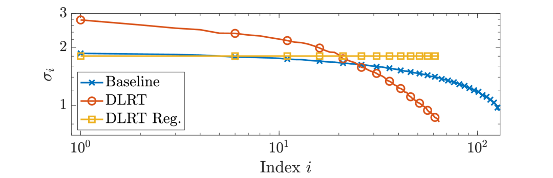
Figure 1: The singular values $\sigma_{i}(W)$ of sequential layer 7 in VGG16 for baseline training, dynamical low-rank training (DLRT), and regularized DLRT with our condition number regularizer $\mathcal{R}$ with $\beta=0.075$. The matrix $W$ is formed as the first-mode unfolding of the convolutional tensor. Conditioning of the regularized low-rank layer is significantly improved compared to the non-regularized low-rank and baseline layer.²

where $\kappa(W^{\ell}):=\left\lVert W^{\ell}\right\rVert\left\lVert W^{\ell,{\dagger}}\right\rVert$ is the condition number of the matrix of layer $\ell$, $W^{\dagger}$ is the pseudo-inverse of a matrix $W$, and $\kappa(\sigma^{\ell})$ is the condition number of the layer activation function $\sigma^{\ell}$. The condition number of the element-wise non-linear activation functions $\sigma^{\ell}$ can be computed with the standard definitions (see trefethen1997numerical and savostianova2023robustlowranktrainingapproximate for condition numbers of several popular activation functions). Equation˜1 allows us to consider each layer individually, thus we drop the superscript $\ell$ for brevity of exposition.

The sensitivity of a low-rank factorized network can be readily deducted from Equation˜1 by leveraging orthonormality of $U,V$: $\kappa(USV^{\top})=\left\lVert USV^{\top}\right\rVert\left\lVert VS^{\dagger}U^{\top}\right\rVert=\left\lVert S\right\rVert\left\lVert S^{\dagger}\right\rVert=\kappa(S)$. This fact allows us to only consider the $r\times r$ coefficient matrix $S$ to control the networks sensitivity. The condition number $\kappa(S)$ can be determined via a singular value decomposition (SVD) of $S$, which is computationally feasible when $r\ll n$.

Adversarial robustness-aware low-rank training: Enhancing the adversarial robustness of the network during low-rank training thus boils down to control the conditioning of $S$, which is a non-trivial task. In fact, the dynamics of the singular spectrum of $S$ of adaptive low-rank training schemes as DLRT steffen2022low exhibit ill conditioned behavior, even if $S$ is always full rank. In Figure˜1, we observe that the singular values a rank 64 factorization of a network layer compressed with DLRT range from $\sigma_{r=1}=2.7785$ to $\sigma_{r=64}=0.8210$ yielding a condition number of $\kappa(S)=3.3844$. In comparison, the baseline network has singular values ranging from $\sigma_{r=1}=1.8627$ to $\sigma_{r=128}=0.9445$ yielding a lower condition number of $\kappa(S)=1.9722$. As a result, a $\ell^{2}$-FGSM attack with strength $\epsilon=0.3$, reduces the accuracy of the baseline network to $54.96\%$, while the low-rank network’s accuracy drops to $43.39\%$, see Table˜2.

Thus, we design a computationally efficient regularizer $\mathcal{R}$ to control and decrease the condition number of each network layer during training. The regularizer $\mathcal{R}$ only acts on the small $r\times r$ coefficient matrices $S$ of each layer and thus has a minimal memory and compute overhead over low-rank training. The regularizer is differentiable almost everywhere and compatible with automatic differentiation tools. Additionally, ${\mathcal{R}}$ has a closed form derivative that enables an efficient and scalable implementation of ${\nabla}{\mathcal{R}}$. Furthermore, ${\mathcal{R}}$ compatible with any rank-adaptive low-rank training scheme that ensures orthogonality of $U,V$, e.g., zhang2023adalora ; schotthöfer2024federateddynamicallowranktraining ; schotthöfer2024geolorageometricintegrationparameter ; savostianova2023robustlowranktrainingapproximate .

Definition 1.

We define the robustness regularizer ${\mathcal{R}}$ for any $S\in\mathbb{R}^{r\times r}$ by

$${\mathcal{R}}(S)=\|S^{\top}\!S-\alpha_{S}^{2}I\|\qquad\text{where}\qquad\alpha_{S}^{2}=\frac{1}{r}\|S\|^{2}$$ (2)

and $I=I_{r}$ is the $r\times r$ identity matrix.

The regularizer ${\mathcal{R}}$ can be viewed as an extension of the soft orthogonal regularizer xie2017all ; bansal2018can where we penalize the distance of $S^{\top}\!S$ to the well-conditioned matrix $\alpha_{S}^{2}I$. Here $\alpha_{S}$ is chosen such that $\|S\|=\|\alpha_{S}I\|$. Moreover, ${\mathcal{R}}$ is also a scaled standard deviation of the set $\{\sigma_{i}(S)^{2}\}_{i=1}^{r}$, that is,

$$\frac{1}{r}{\mathcal{R}}(S)^{2}=\frac{1}{r}\sum_{i=1}^{r}(\sigma_{i}(S)^{2})^{2}-\Big{(}\frac{1}{r}\sum_{i=1}^{r}\sigma_{i}(S)^{2}\Big{)}^{2}.$$ (3)

See Appendix˜B for the proof. Therefore, ${\mathcal{R}}$ is a unitarily invariant regularizer; namely, ${\mathcal{R}}(USV^{\top})={\mathcal{R}}(S)$ for orthogonal $U,V$. These two forms of ${\mathcal{R}}$ are useful in the properties shown below.

Proposition 1.

The gradient of ${\mathcal{R}}$ in (2) is given by ${\nabla}{\mathcal{R}}(S)=2S(S^{\top}\!S-\alpha_{S}^{2}I)/\mathcal{R}(S)$.

See Appendix˜B for the proof. The gradient computation consists only of $r\times r$ matrix multiplications and an Frobenius norm evaluation, and is thus computationally efficient for $r\ll m$. Further, its closed form enables a straight-forward integration into existing optimizers as Adam or SGD applied to $S$.

Table 1: VGG16 on UCM data. Comparison of adversarial robustness of LoRA and DLRT trained networks under the $\ell^{2}$-FGSM attack with similar compression rate. Orthogonality of $U,V$ increases adversarial performance significantly.

Method	c.r. [%]	clean Acc [%]	$\ell^{2}$-FGSM, $\epsilon=0.1$
RobustDLRT, $\beta=0.0$	95.30	93.92	72.41
RobustDLRT, $\beta=0.075$	95.84	94.61	78.68
LoRA, $\beta=0.075$	95.83	88.57	73.81

Proposition 2.

We have the condition number bound

$$\kappa(S)\leq\exp\bigg{(}\frac{1}{\sqrt{2}\sigma_{r}(S)^{2}}{\mathcal{R}}(S)\bigg{)}$$ (4)

for any $S\in\mathbb{R}^{r\times r}$.

See Appendix˜B for the proof. Thus, if $\sigma_{r}(S)$ is not too small, we can use ${\mathcal{R}}(S)$ as a good measure for the conditioning of $S$. Note that the singular value truncation of Algorithm˜1 ensures that $\sigma_{r}(S)$ is always sufficiently large. Figure˜2a) and b) show the dynamics of ${\mathcal{R}}(S(t))$ and $\kappa(S(t))$ during regularized training using Algorithm˜1, and we see that $\kappa(S(t))$ decays as ${\mathcal{R}}(S(t))$ decays, validating ˜2.

Remark 1.

When $U,V$ are not orthonormal, e.g. in simultaneous gradient descent training (LoRA), we have ${\mathcal{R}}(USV^{\top})\not={\mathcal{R}}(S)$. $USV^{\top}$ are zero-valued thus the bound of Equation˜4 is not useful. Table˜1 shows that the clean accuracy and adversarial accuracy of regularized LoRA is significantly lower than baseline training or regularized training with orthonormal $U,V$.

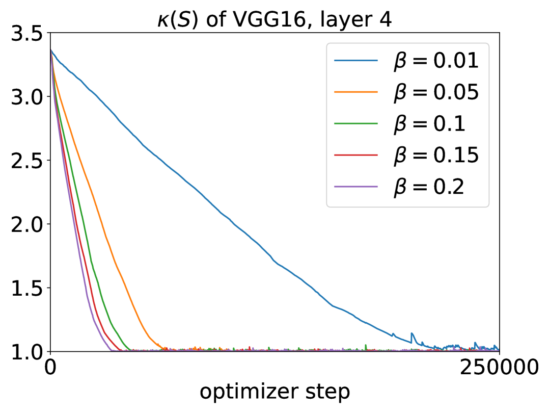
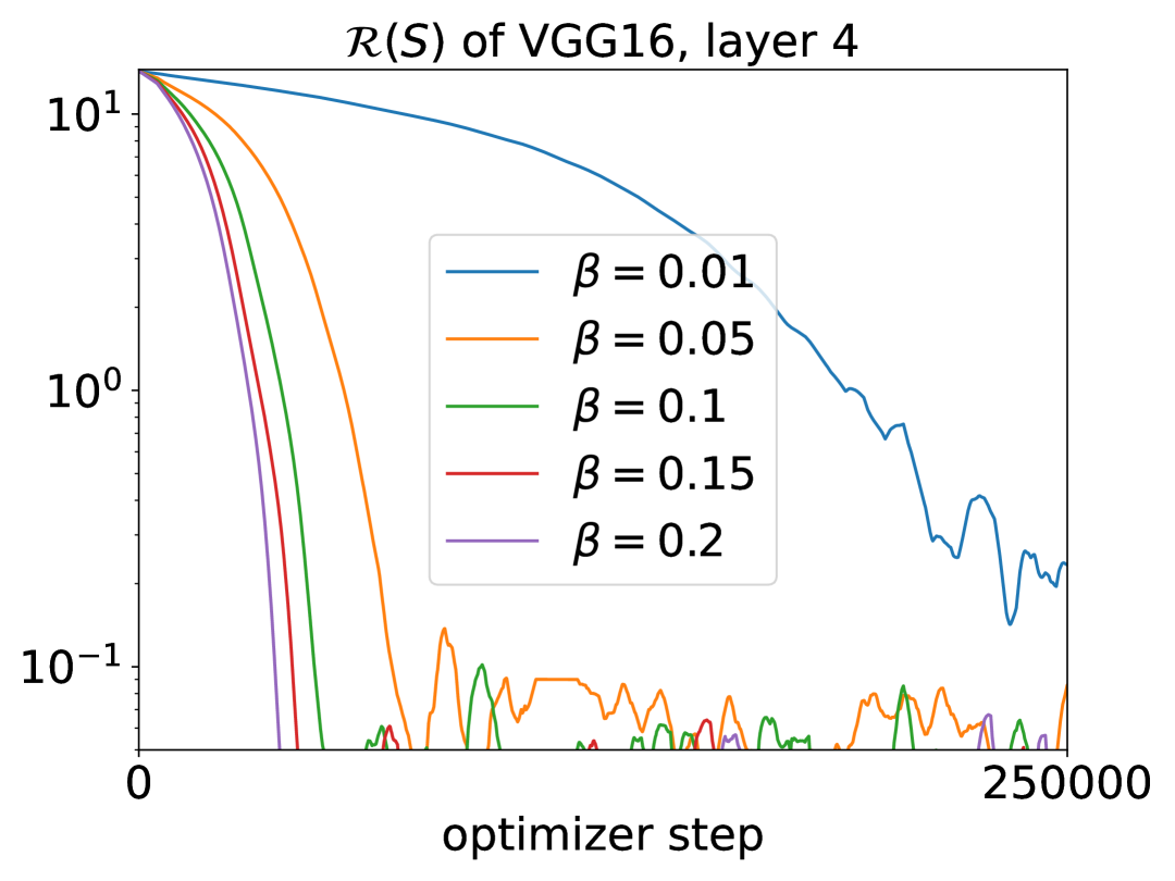
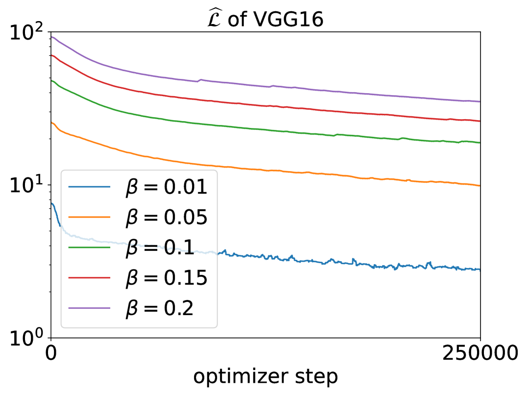
Figure 2: UCM Dataset, $\kappa(S(t))$ and $\mathcal{R}(S(t))$ of layer 4 of VGG16 for different regularizations strengths $\beta$. Each line is the median of 5 training runs. Higher $\beta$ values lead to faster reduction of the layer condition $\kappa(S)$, which quickly approaches its minimum value $1$, and faster decay of $\mathcal{R}$. Unregularized training, i.e. $\beta=0$ leads to $\kappa(S)>1e3$ after few iterations.

We now study the stability of the regularizer when applied to a least squares regression problem, i.e., given a fixed $W\in\mathbb{R}^{r\times r}$ we seek to minimize $\mathcal{J}(S):=\beta{\mathcal{R}}(S)+\frac{1}{2}\|S-W\|^{2}$ over $S\in\mathbb{R}^{r\times r}$.

Proposition 3.

For a fixed $W\in\mathbb{R}^{r\times r}$, consider the dynamical system $\dot{S}(t)+\beta{\nabla}{\mathcal{R}}(S(t))+S(t)=W$. Then for any $t\geq 0$ we have the long-time stability estimate

$$\tfrac{1}{2}\|S(t)-W\|^{2}+2\beta\int_{0}^{t}e^{\tau-t}{\mathcal{R}}(S(\tau))\,\mathrm{d}\tau\leq\tfrac{1}{2}e^{-t}\|S(0)-W\|^{2}+2(1-e^{-t})\beta(1+2\beta)\|W\|^{2}.$$ (5)

See Appendix˜B for the proof. We note that unlike standard ridge and lasso regularizations methods, ${\mathcal{R}}$ lacks convexity; thus long-time stability of the regularized dynamics is not obvious. However, ${\nabla}{\mathcal{R}}$ possesses monotonicity properties that we leverage to show in (5) that the growth in ${\mathcal{L}}$ in the regularized problem only depends on $\beta$, $W$, and the initial loss. Moreover, for large $t$, the change in the final loss by the regularizer only depends on $\beta$ and the true solution $W$ and not the specific path $S(t)$. While training on the non-convex loss will not provide the same theoretical properties as the least-square loss, ˜3 and the experiments in Figure˜2 give confidence that adding our regularizer does not yield a relatively large change in the loss decay rate over moderate training regimes. Particularly, we observe empirically in Figure˜2 that the condition number $\kappa(S)$ of decreases alongside the regularizer value $\mathcal{R}$ during training.

Remark 2.

We note ${\mathcal{R}}^{2}$ can also be used in place of ${\mathcal{R}}$. While ${\mathcal{R}}^{2}$ is differentiable at ${\mathcal{R}}(S)=0$, we choose ${\mathcal{R}}$ as our regularizer due to the proper scaling in (4).

4 A rank-adaptive, adversarial robustness increasing dynamical low-rank training scheme

In this section we integrate the regularizer $\mathcal{R}$ into a rank-adaptive, orthogonality preserving, and efficient low-rank training scheme. We are specifically interested in a training method that 1) enables separation of the spectral dynamics of the coefficients $S$ from the bases $U,V$ and 2) ensures orthogonality of $U,V$ at all times during training to obtain control layer conditioning in a compute and memory efficient manner. Popular schemes based upon simultaneous gradient descent of the low-rank factors such as LoRA hu2021lora are not suitable here. These methods typically do not ensure orthogonality of $U$ and $V$. Consequently, $\mathcal{R}(USV^{\top})\not=\mathcal{R}(S)$, and this fact renders evaluation of the regularizer $\mathcal{R}$ computationally inefficient.

Thus we adapt the two-step scheme of schotthöfer2024federateddynamicallowranktraining which ensures orthogonality of $U,V$. The method dynamically reduces or increases the rank of the factorized layers dynamically depending on the training dynamics and the complexity of the learning problem at hand. Consequently, the rank of each layer is no longer a hyper-parameter that needs fine-tuning, c.f. hu2021lora ; savostianova2023robustlowranktrainingapproximate , but is rather an interpretable measure for the inherent complexity required for each layer.

To facilitate the discussion, we define $\widetilde{\mathcal{L}}=\mathcal{L}+\beta\mathcal{R}$ as the regularized loss function of the training process with regularization parameter $\beta>0$. To construct the method we consider the (stochastic) gradient descent-based update of a single weight matrix $W_{t+1}=W_{t+1}-\lambda\nabla_{W}\widetilde{\mathcal{L}}$ for minimizing $\widetilde{\mathcal{L}}$ with step size $\lambda>0$. The corresponding continuous time gradient flow reads $\dot{W}(t)=-\nabla_{W}\widetilde{\mathcal{L}}(W(t))$, which is a high-dimensional dynamical system with a steady state solution. We draw from established dynamical low-rank approximation (DLRA) methods, which were initially proposed for matrix-valued equations KochLubich07 . DLRA was recently extended to neural network training steffen2022low ; zangrando2023rank ; schotthöfer2024federateddynamicallowranktraining ; schotthöfer2024geolorageometricintegrationparameter ; kusch2025augmentedbackwardcorrectedprojectorsplitting ; Hnatiuk to formulate a consistent gradient flow evolution for the low-rank factors $U$, $S$, and $V$.

The DLRA method constrains the trajectory of $W$ to the manifold $\mathcal{M}_{r}$, consisting of $n\times n$ matrices with rank $r$, by projecting the full dynamics $\dot{W}$ onto the local tangent space of $\mathcal{M}_{r}$ via an orthogonal projection, see Figure˜3. The low-rank matrix is represented as $USV^{\top}\in\mathcal{M}_{r}$, where $U\in\mathbb{R}^{n\times r}$ and $V\in\mathbb{R}^{n\times r}$ have orthonormal columns and $S\in\mathbb{R}^{r\times r}$ is full-rank (but not necessarily diagonal). An explicit representation of the tangent space leads to equations for the factors $U$, $S$, and $V$ in (KochLubich07, , Proposition 2.1). However, following these equations requires a prohibitively small learning rate due to the curvature of the manifold lubich2014projector . Therefore, specialized integrators have been developed to accurately navigate the manifold with reasonable learning rates lubich2014projector ; ceruti2022unconventional ; ceruti2022rank .

Below we summarize proposed method, called RobustDLRT, along with the changes induced by adding our robustness regularizer. A single iteration of DLRT is specified in Algorithm˜1.

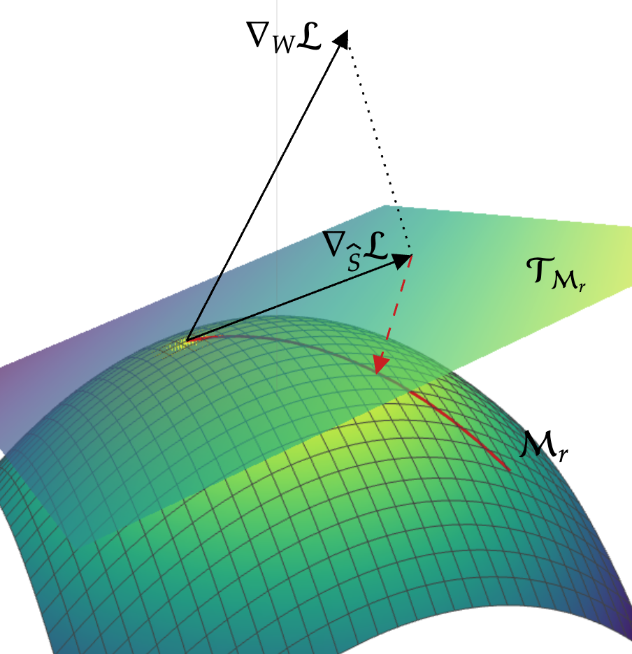
Figure 3: Geometric interpretation of Algorithm˜1. First, we compute the parametrization of the tangent plane $\mathcal{T}_{\mathcal{M}_{r}}$. Then we compute the projected gradient update with $\nabla_{\widehat{S}}\mathcal{L}$. Lastly, we retract the updated coefficients back onto the manifold $\mathcal{M}_{r}$. The regularizer $\mathcal{R}$ effectively changes the local curvature of $\mathcal{M}_{r}$.

Basis Augmentation:

The method first augments the current bases $U^{t},V^{t}$ at optimization step $t$ by their gradient dynamics $\nabla_{U}\mathcal{L}$, $\nabla_{V}\mathcal{L}$ via

$$\begin{aligned} {\widehat{U}}&=\texttt{orth}([U^{t}\mid\nabla_{U}\mathcal{L}(U^{t}S^{t}V^{t,\top})])\in\mathbb{R}^{n\times 2r},\\ {\widehat{V}}&=\texttt{orth}([V^{t}\mid\nabla_{V}\mathcal{L}(U^{t}S^{t}V^{t,\top})])\in\mathbb{R}^{n\times 2r},\end{aligned}$$ (6)

to double the rank of the low-rank representation and subsequently creates orthonormal bases ${\widehat{U}},{\widehat{V}}$. Since ${\mathcal{R}}(USV^{\top})={\mathcal{R}}(S)$, $\nabla_{U}{\mathcal{R}}(USV^{\top})=\nabla_{V}{\mathcal{R}}(USV^{\top})=0$; hence $\nabla_{U}\widetilde{\mathcal{L}}=\nabla_{U}\mathcal{L}$ and $\nabla_{V}\widetilde{\mathcal{L}}=\nabla_{V}\mathcal{L}$ are used in (6). The span on ${\widehat{U}}$ contains $U$, which is needed to ensure of the loss does not increase during augmentation, and a first-order approximation of the basis for $W^{t+1}$ using the exact gradient flow for $U$, see (schotthöfer2024federateddynamicallowranktraining, , Theorem 2) for details. Geometrically, the augmented space

$$\mathcal{S}=\{{\widehat{U}}Z{\widehat{V}}^{\top}:Z\in\mathbb{R}^{2r\times 2r}\}$$ (7)

can be seen as subspace of the tangent plane of $\mathcal{M}_{r}$ at $U^{t}S^{t}V^{t,\top}$, see Figure˜3.

Latent Space Training:

We update the augmented coefficients ${\widehat{S}}$ via a Galerkin projection of the training dynamics onto the latent space $\mathcal{S}$. The augmented coefficients ${\widehat{S}}$ are updated by integrating the projected gradient flow $\dot{{\widehat{S}}}=-{\widehat{U}}^{\top}\nabla_{W}\widetilde{\mathcal{L}}{\widehat{V}}=-\nabla_{\widehat{S}}\widetilde{\mathcal{L}}$ using stochastic gradient descent or an other suitable optimizer for a number of $s_{*}$ local iterations, i.e.

$${{\widehat{S}}_{s+1}} ={\widehat{S}}_{s}-\lambda\nabla_{\widehat{S}}\mathcal{L}-\beta\nabla_{\widehat{S}}\mathcal{R}({\widehat{S}}_{s}),$$ (8)

Equation˜8 is initialized with ${{\widehat{S}}_{0}}={\widehat{U}}^{\top}U^{t}S^{t}V^{t,\top}{\widehat{V}}\in\mathbb{R}^{2r\times 2r}$, and we set $\tilde{S}=\hat{S}_{s_{*}}$

Truncation:

Finally, the augmented solution ${\widehat{U}}\tilde{S}{\widehat{V}}^{\top}$ is retracted back onto the manifold $\mathcal{M}_{r}$. The retraction can be computed efficiently by using a truncated SVD of $\tilde{S}$ that discards the smallest $r$ singular values. To enable rank adaptivity, the new rank $r_{1}$ instead of $r$ can be chosen by a variety of criteria, e.g., a singular value threshold $\left\lVert[\sigma_{r_{1}},\dots,\sigma_{2r}]\right\rVert_{2}<\vartheta$. Once a suitable rank is determined, the bases $U$ and $V$ are updated by discarding the basis vectors corresponding to the truncated singular values.

Computational cost:

The computational cost of the above described scheme is asymptotically the same as LoRA, since the reconstruction of the full weight matrix $W$ is never required. The orthonormalization accounts for $\mathcal{O}(nr^{2})$, the regularizer $\mathcal{R}$ for $\mathcal{O}(r^{3})$, and the SVD for $\mathcal{O}(r^{3})$ floating point operations. When using multiple coefficient update steps $s_{*}>1$, the amortized cost is indeed lower than that of LoRA, since only the gradient w.r.t ${\widehat{S}}$ is required in most updates.

1

Input : Initial orthonormal bases $U,V\in\mathbb{R}^{n\times r}$ and diagonal $S\in\mathbb{R}^{r\times r}$;

$\vartheta$: singular value threshold for rank truncation; $\lambda$: learning rate.

Evaluate $\mathcal{L}(USV^{\top})$

  /* Forward evaluate */

$G_{U}\leftarrow\nabla_{U}\mathcal{L}(USV^{\top});\,G_{V}\leftarrow\nabla_{V}\mathcal{L}(USV^{\top})$

  /* Backprop on basis */

2

${\widehat{U}}\leftarrow\texttt{orth}([U\mid G_{U}])$; ${\widehat{V}}\leftarrow\texttt{orth}([V\mid G_{V}])$

  /* augmentation in parallel */

${\widehat{S}}\leftarrow{\widehat{U}}^{\top}USV^{\top}{\widehat{V}}$

  /* coefficient augmentation */

${\widehat{S}}\leftarrow\texttt{coefficient\_update}({\widehat{S}},s_{*},\lambda,\beta)$

  /* regularized coefficient training */

3 $U,S,V\leftarrow$truncation$({\widehat{S}},{\widehat{U}},{\widehat{V}})$

4 def  coefficient_update(${\widehat{S}}_{0}$: coefficient, $s_{*}$: # local steps, $\lambda$: learning rate, $\beta$: robustness regularization weight):

5    for $s=1,\dots,s_{*}$ do

6       $G_{S}\leftarrow-\lambda\nabla_{\widehat{S}}\mathcal{L}({\widehat{U}}{\widehat{S}}_{s-1}{\widehat{V}}^{\top})-\beta\nabla_{{\widehat{S}}_{s}}\mathcal{R}({\widehat{S}}_{s})$

       ${\widehat{S}}_{s}\leftarrow{\widehat{S}}_{s-1}+\texttt{optim}(G_{S})$

        /* optimizer update, e.g., SGD or Adam */

7      

8    return ${\widehat{S}}_{s_{*}}$

9 def  truncation(${\widehat{S}}$: augmented coefficient, ${\widehat{U}}$: augmented basis, ${\widehat{V}}$: augmented co-basis ):

10    $P_{r_{1}},\Sigma_{r_{1}},Q_{r_{1}}\leftarrow$ truncated svd$(\widetilde{S})$ with threshold $\vartheta$ to new rank $r_{1}$

    $U\leftarrow{\widehat{U}}P_{r_{1}}$; $V\leftarrow{\widehat{V}}Q_{r_{1}}$

     /* Basis update */

    $S\leftarrow\Sigma_{r_{1}}$

     /* Coefficient update with diagonal $\Sigma_{r_{1}}$ */

11    return $U,S,V$

12   

Algorithm 1 Single iteration of RobustDLRT.

4.1 Extension to convolutional neural networks

The convolution layer map in 2D CNNs translates a $W\times H$ image with $N_{I}$ in-features to $N_{O}$ out-features. Using tensors, this map is expressed as $Y=C*X$ where $X\in\mathbb{R}^{N_{I}\times W\times H}$, $Y\in\mathbb{R}^{N_{O}\times W\times H}$, and $C\in\mathbb{R}^{N_{O}\times N_{I}\times S_{W}\times S_{H}}$ is the convolutional kernel with a convolution window size $S_{W}\times S_{H}$. Neglecting the treatment of strides and padding, $C*X$ is given as a tensor contraction by

$$Y(o,w,h)=\textstyle\sum_{c,s_{w},s_{h}}C(o,c,s_{w},s_{h})X(c,w+s_{w},h+s_{h})$$ (9)

where $s_{w}$ and $s_{h}$ range from $-S_{W}/2,\ldots,S_{W}/2$ and $-S_{H}/2,\ldots,S_{H}/2$ respectively, and $o=1,\dots,N_{O}$, $w=1,\dots,W$, and $h=1,\dots,H$.

DLRT was extended to convolutional layers in zangrando2023rank by compressing $C$ with a Tucker factorization. Little is gained in compressing the window modes as they are traditionally small. Thus, we only factorize $C$ in the feature modes with output and input feature ranks $r_{O}\ll N_{O}$ and $r_{I}\ll N_{I}$ as

$$C(o,i,s_{w},s_{h})=\textstyle\sum_{q_{O},q_{I}=1}^{r_{I},r_{O}}U_{O}(o,q_{O})U_{I}(i,q_{I})S(q_{O},q_{I},s_{w},s_{h}).$$ (10)

Substituting (10) into (9) and rearranging indices yields

$$Y(o,w,h) =\textstyle\sum_{q_{O}}U_{O}(o,q_{O})\widetilde{Y}(q_{O},w,h),$$ (11a)

$$\widetilde{Y}(q_{O},w,h) =\textstyle\sum_{q_{I},s_{w},s_{h}}S(q_{O},q_{I},s_{w},s_{h})\widetilde{X}(q_{I},w+s_{w},h+s_{h}),$$ (11b)

$$\widetilde{X}(q_{I},w+s_{w},h+s_{h}) =\textstyle\sum_{c}U_{I}(c,q_{I})X(c,w+s_{w},h+s_{h}).$$ (11c)

Remark 3.

Aside from the prolongation (11a) and retraction (11c) from/to the low-rank latent space, the low-rank convolution map (11) equations features a convolution (11b) similar to (9) but in the reduced dimension low-rank latent space.

Robustness regularization for convolutional layers.

The contractions in (9) and (11b) show that the output channels arise from a tensor contraction of the input channel and window modes; hence, both (9) and (11b) can be viewed as matrix-vector multiplication where $C$ is matricised on the output channel mode; i.e., $C\to\text{Mat}(C)\in\mathbb{R}^{N_{O}\times N_{I}S_{W}S_{H}}$ and $S\to\text{Mat}(S)\in\mathbb{R}^{r_{O}\times r_{I}S_{W}S_{H}}$. Therefore, we only regularize $\text{Mat}(S)$ with our robustness regularizer. Moreover, we assume $r_{O}\leq r_{I}S_{W}S_{H}$, which is almost always the case since $r_{O}$ and $r_{I}$ are comparable and $S_{W}S_{H}\gg 1$. Then we regularize convolutional layers by ${\mathcal{R}}(\text{Mat}(S)^{\top})$ so that $SS^{\top}$ is an $r_{O}\times r_{O}$ matrix, which is computationally efficient.

We remark, that the extension of Algorithm˜1 to a tensor-valued layer with Tucker factorization only requires to change the truncation step; the SVD is replaced by a truncated Tucker decomposition of $S$. The Tucker bases $U_{i}$ can be augmented in parallel analogously to $U,V$ in the matrix case.

Table 2: UCM and Cifar10 benchmark. Clean and adversarial accuracy means and std. devs. of the baseline and regularized low-rank networks for different architectures. We report the low-rank results for unregulated, $\beta=0.0$, and the best performing $\beta$, given in Table˜6. Algorithm˜1 is able to match or surpass baseline adversarial accuracy values at compression rates of up to $95\%$ in most setups.

UCM Data			Clean	Acc [%] for $\ell^{2}$-FGSM, $\epsilon$			Acc [%] for Jitter, $\epsilon$		Acc [%] for Mixup, $\epsilon$
	Method	c.r. [%]	Acc. [%]	0.05	0.1	0.3	0.035	0.045	0.025	0.1	0.75
VGG16	Baseline	0.0	94.40$\pm$0.72	86.71$\pm$1.90	76.40$\pm$2.84	54.96$\pm$2.99	89.58$\pm$2.99	85.05$\pm$3.40	77.77$\pm$1.61	37.25$\pm$3.66	23.05$\pm$3.01
	DRLT	95.30	93.92$\pm$0.23	87.95$\pm$1.02	72.41$\pm$2.08	43.39$\pm$4.88	83.99$\pm$1.22	67.41$\pm$1.63	85.79$\pm$1.51	40.42$\pm$2.89	20.13$\pm$2.92
	RobustDLRT	95.84	94.61$\pm$0.35	89.12$\pm$1.33	78.68$\pm$2.30	53.30$\pm$3.14	88.33$\pm$1.20	79.81$\pm$0.93	90.33$\pm$0.90	70.12$\pm$3.08	47.31$\pm$2.78
VGG11	Baseline	0.0	94.23$\pm$0.71	89.93$\pm$1.33	78.66$\pm$2.46	39.45$\pm$2.98	90.25$\pm$1.66	85.24$\pm$1.90	83.10$\pm$1.47	40.34$\pm$4.88	22.01$\pm$3.21
	DRLT	94.89	93.70$\pm$0.71	86.58$\pm$1.22	67.55$\pm$2.16	28.92$\pm$2.65	83.90$\pm$1.36	63.41$\pm$1.39	87.15$\pm$1.18	40.17$\pm$4.96	14.18$\pm$3.78
	RobustDLRT	94.59	93.57$\pm$0.84	87.90$\pm$0.91	72.96$\pm$1.55	32.85$\pm$2.46	86.77$\pm$0.76	74.31$\pm$1.50	88.00$\pm$1.13	60.97$\pm$4.18	28.56$\pm$3.64
ViT-32b	Baseline	0.0	96.72$\pm$0.36	93.02$\pm$0.38	92.18$\pm$0.31	89.71$\pm$0.28	93.71$\pm$1.22	93.21$\pm$1.17	89.62$\pm$1.81	51.05$\pm$3.17	43.91$\pm$3.97
	DRLT	86.7	96.38$\pm$0.60	91.21$\pm$0.44	82.10$\pm$0.32	62.45$\pm$0.41	86.67$\pm$1.05	79.81$\pm$0.81	80.48$\pm$1.82	41.52$\pm$3.24	35.91$\pm$3.76
	RobustDLRT	87.9	96.41$\pm$0.67	92.57$\pm$0.34	85.67$\pm$0.41	69.94$\pm$0.42	91.03$\pm$0.86	84.19$\pm$1.39	87.33$\pm$1.81	46.39$\pm$2.75	40.76$\pm$3.88
Cifar10 Data
VGG16	Baseline	0.0	89.82$\pm$0.45	76.22$\pm$1.38	63.78$\pm$2.01	34.97$\pm$2.54	78.60$\pm$1.12	73.54$\pm$1.55	71.51$\pm$1.31	37.36$\pm$2.60	16.12$\pm$2.12
	DRLT	94.37	89.23$\pm$0.62	74.07$\pm$1.23	59.55$\pm$1.79	28.74$\pm$2.21	72.51$\pm$1.04	66.21$\pm$1.41	79.56$\pm$1.15	59.88$\pm$2.26	38.98$\pm$1.94
	RobustDLRT	94.18	89.49$\pm$0.58	76.04$\pm$1.18	62.08$\pm$1.69	32.77$\pm$2.04	75.53$\pm$0.98	69.93$\pm$1.22	87.62$\pm$1.07	84.80$\pm$2.01	81.26$\pm$2.15
VGG11	Baseline	0.0	88.34$\pm$0.49	75.89$\pm$1.42	64.21$\pm$1.96	31.76$\pm$2.45	74.96$\pm$1.09	68.59$\pm$1.63	74.77$\pm$1.26	40.88$\pm$2.58	08.95$\pm$1.98
	DRLT	95.13	88.13$\pm$0.56	72.02$\pm$1.34	55.83$\pm$1.92	21.59$\pm$2.16	66.98$\pm$1.05	58.57$\pm$1.55	79.42$\pm$1.08	47.95$\pm$2.18	22.92$\pm$1.77
	RobustDLRT	94.67	87.97$\pm$0.52	76.04$\pm$1.26	63.82$\pm$1.83	30.77$\pm$2.30	71.06$\pm$1.00	65.63$\pm$1.38	84.93$\pm$1.10	78.35$\pm$1.89	65.93$\pm$2.04
ViT-32b	Baseline	0.0	95.42$\pm$0.35	79.94$\pm$0.95	63.66$\pm$1.62	32.09$\pm$2.05	84.65$\pm$0.88	77.20$\pm$1.04	52.17$\pm$1.49	16.03$\pm$2.34	13.29$\pm$2.01
	DRLT	73.42	95.39$\pm$0.41	79.50$\pm$0.91	61.62$\pm$1.48	30.32$\pm$1.94	83.33$\pm$0.80	76.16$\pm$0.95	58.32$\pm$1.44	17.43$\pm$2.28	14.49$\pm$1.92
	RobustDLRT	75.21	94.66$\pm$0.38	82.03$\pm$0.88	69.29$\pm$1.43	38.05$\pm$1.99	87.97$\pm$0.75	83.03$\pm$0.91	74.49$\pm$1.32	27.80$\pm$2.11	18.34$\pm$1.87

5 Numerical Results

We evaluate the numerical performance of Algorithm˜1 compared with non-regularized low-rank training, baseline training, and several other robustness-enhancing methods on various datasets and network architectures. We measure the compression rate (c.r.) as the relative amount of pruned parameters of the target network, i.e. $\textup{c.r.}=(1-\frac{\#\textup{params low-rank net}}{\#\textup{params baseline net}})\times 100$. Detailed descriptions of the models, data-sets, pre-processing, training hyperparameters, and competitor methods are given in Appendix˜A. The reported numbers in the tables represent the average over 10 stochastic training runs. We observe in Table˜2 that clean accuracy results exhibit a standard deviation of less than 0.8%; the standard deviation increases with the attack strength $\epsilon$ for all tests and methods. This observation holds true for all presented results, thus we omit the error bars in the other tables for the sake of readability.

UCM dataset: We observe in Table˜2 that Algorithm˜1 can compress the VGG11, VGG16 and ViT-32b networks equally well as the non-regularized low-rank compression and achieves the first goal of high compression values of up to $95\%$ reduction of trainable parameters. Furthermore, the clean accuracy is similar to the non-compressed baseline architecture; thus, we achieve the second goal of (almost) loss-less compression. Noting the adversarial accuracy results under the $\ell^{2}$-FGSM, Jitter, and Mixup attacks with various attack strengths $\epsilon$, we observe that across all tests, the regularized low-rank network of Algorithm˜1 significantly outperforms the non-regularized low-rank network. For the $\ell^{2}$-FGSM attack, our method is able to recover the adversarial accuracy of the baseline network. For Mixup, the regularization almost doubles the baseline accuracy for VGG16. By targeting the condition number of the weights, which gives a bound on the relative growth of the loss w.r.t. the size of the input, we postulate that the large improvement could be attributed to the improved robustness against the scale invariance attack (lin2020nesterov, , Section 3.3) included in MixupWe refer the reader to Section˜A.1.4 for a precise definition of the Mixup attack featuring scale invariance. However, this hypothesis was not further explored and is delayed to a future work. Finally, we are able to recover half of the lost accuracy in the Jitter attack. Overall, we achieved the third goal of significantly increasing adversarial robustness of the compressed networks. We refer to Table˜6 for the used values of $\beta$ and to Section˜A.3 for extended numerical results for a grid of different $\beta$ values.

Table 3: Comparison to literature on CIFAR10 with VGG16 under the $\ell^{1}$-FGSM. The first three rows list the computed mean over $10$ random initializations. The values of all other methods, given below the double rule, are taken from (NEURIPS2024_ea48cb23, , Table 1). RobustDLRT has higher adversarial accuracy at higher compression rates than all listed methods.

		$\ell^{1}$-FGSM, $\epsilon$
Method	c.r. [%]	0.0	0.002	0.004	0.006
RobustDLRT $\beta=0.15$	94.35	89.35	78.72	66.02	54.15
DLRT	94.58	89.55	74.71	59.61	47.56
Baseline	0	89.83	78.61	64.66	53.71
Cayley SGD li2020efficientriemannianoptimizationstiefel	0	89.62	74.46	58.16	45.29
Projected SGD Projection_like_Retractions	0	89.70	74.55	58.32	45.74
CondLR savostianova2023robustlowranktrainingapproximate $\xi=0.5$	50	89.97	72.25	60.19	50.17
CondLR savostianova2023robustlowranktrainingapproximate $\xi=0.5$	80	89.33	68.23	48.54	36.66
LoRA hu2021lora	50	89.97	67.71	48.86	38.49
LoRA hu2021lora	80	88.10	64.24	42.66	29.90
SVD prune yang2020learninglowrankdeepneural	50	89.92	67.30	47.77	36.98
SVD prune yang2020learninglowrankdeepneural	80	87.99	63.57	42.06	29.27

Cifar10 dataset: We repeat the methodology of the UCM dataset for Cifar10, and observe similar computational results in Table˜2. Furthermore, we compare our method in Table˜3 to several methods of the recent literature, see Section˜2. We compare the adversarial accuracy under the $\ell^{1}$-FGSM attack, see Section˜A.1.2 for details, for consistency with the literature results. We find that our proposed method achieves the highest adversarial validation accuracy for all attack strengths $\epsilon$, even surpassing the baseline adversarial accuracy. Additionally, we find an at least 15% higher compression ratio with RobustDLRT than the second best compression method, CondLR savostianova2023robustlowranktrainingapproximate .

Table 4: UCM dataset – Black-box attack. Adversarial images with the $\ell^{2}$-FGSM attack are generated by the baseline network for different values of $\epsilon$. The baseline, low-rank, and regularized low-rank networks are evaluated on these images. Regularized low-rank compression achieves high adversarial accuracy, even under strong attacks.

			$\ell^{2}$-FGSM, $\epsilon$
	Method	c.r. [%]	0.05	0.1	0.25	0.05	0.75	1.0
VGG16	Baseline	0.0	86.71	76.40	48.76	39.33	35.23	33.23
	$\beta=0$	95.30	93.03	91.81	88.09	83.14	78.95	76.00
	$\beta=0.05$	95.15	92.66	92.47	91.33	88.76	86.85	84.76
VGG11	Baseline	0.0	89.93	78.66	60.76	45.23	38.38	35.52
	$\beta=0$	95.82	92.76	91.81	88.25	84.09	80.57	77.71
	$\beta=0.05$	96.12	92.95	92.66	92.00	91.04	88.66	87.33

Black-box attacks: We investigate the scenario, where an attacker has knowledge of the used model architecture, but not of the low-rank compression. We use the Imagenet-1k pretrained VGG16 and VGG11 and re-train it with Algorithm˜1 and baseline training on the UCM data using the same training hyperparameters. Then we generate adversarial examples with the baseline network and evaluate the performance on the low-rank network with and without regularization. The results are given in Table˜4. In this scenario, the weights from low-rank training, being sufficiently far away from the baseline, provide an effective defense against the attack. Further, the proposed regularization significantly improves the adversarial robustness when compared to the unregularized low-rank network. Even for extreme attacks with $\epsilon=1$, the regularized network achieves $84.76\%$ and $87.33\%$ accuracy for VGG16 and VGG11 respectively.

6 Conclusion

RobustDLRT enables highly compressed neural networks with strong adversarial robustness by controlling the spectral properties of low-rank factors. The method is efficient and rank-adaptive that yields an over 94% parameter reduction across diverse models and attacks. The method achieves competitive accuracy, even for strong adversarial attacks, surpassing the current literature results by a significant margin. Therefore, we conclude the proposed method scores well in the combined metric of compression, accuracy and adversarial robustness.

The accomplished high compression and adversarial robustness advance computer vision models and enable broader applications on resource-constrained edge devices. These achievements also enhance energy efficiency and trustworthiness, positively impacting society. The regularization and condition number bounds further improve interpretability, which is crucial for transparency and accountability in critical decision-making when applying the proposed methods.

Funding Acknowledgements

This material is based upon work supported by the Laboratory Directed Research and Development Program of Oak Ridge National Laboratory (ORNL), managed by UT-Battelle, LLC for the U.S. Department of Energy under Contract No. De-AC05-00OR22725.

This manuscript has been authored by UT-Battelle, LLC under Contract No. DE-AC05-00OR22725 with the U.S. Department of Energy. The United States Government retains and the publisher, by accepting the article for publication, acknowledges that the United States Government retains a non-exclusive, paid-up, irrevocable, world-wide license to publish or reproduce the published form of this manuscript, or allow others to do so, for United States Government purposes. The Department of Energy will provide public access to these results of federally sponsored research in accordance with the DOE Public Access Plan(http://energy.gov/downloads/doe-public-access-plan).

This research used resources of the Compute and Data Environment for Science (CADES) at the Oak Ridge National Laboratory, which is supported by the Office of Science of the U.S. Department of Energy under Contract No. DE-AC05-00OR22725"

Appendix A Details to the numerical experiments of this work

A.1 Recap of adversarial attacks

In the following we provide the defintions of the used adversarial attacks. We use the implementation of https://github.com/YonghaoXu/UAE-RS for the $\ell^{2}$-FGSM, Jitter, and Mixup attack. For the $\ell^{1}$-FGSM attack, we use the implementation of https://github.com/COMPiLELab/CondLR.

A.1.1 $\ell^{2}$-FGSM attack

The Fast Gradient Sign Method (FGSM)[17] is a single-step adversarial attack that perturbs an input in the direction of the gradient of the loss with respect to the input. Given a neural network classifier $f_{\theta}$ with parameters $\theta$, an input $x$, and its corresponding label $y$, the attack optimizes the cross-entropy loss $\mathcal{L}_{\text{CE}}(f_{\theta}(x),y)$ by modifying $x$ along the gradient’s sign. The adversarial example is computed as:

$$x^{\prime}=x+\alpha\cdot\frac{\nabla_{x}\mathcal{L}_{\text{CE}}(f_{\theta}(x),y)}{\|\nabla_{x}\mathcal{L}_{\text{CE}}(f_{\theta}(x),y)\|_{\infty}},$$ (12)

where $\alpha$ controls the perturbation magnitude. To ensure the perturbation remains bounded, the difference $x^{\prime}-x$ is clamped by an $\epsilon$ bound, i.e.,

$$x^{\prime}=x+\max(-\epsilon,\min(x^{\prime}-x,\epsilon)).$$ (13)

In this work we fix $\alpha=\epsilon$. The attack can be iterated to increase its strength.

A.1.2 $\ell^{1}$-FGSM attack

The $\ell^{1}$-FGSM attack [37] is used in the reference work of [29] and uses the same workflow as (A.1.1), where (12) is changed to

$$x^{\prime}=x+\alpha\cdot\frac{\textup{sign}(\nabla_{x}\mathcal{L}_{\text{CE}}(f_{\theta}(x),y))}{\Sigma},$$ (14)

where $\Sigma$ denotes the standard deviation of the data-points in the training data-set and the sign of the gradient matrix is taken element wise.

A.1.3 Jitter attack

The Jitter attack [33] is an adversarial attack that perturbs an input by modifying the softmax-normalized output of the model with random noise before computing the loss. Given a neural network classifier $f_{\theta}$ with parameters $\theta$, an input $x$, and its corresponding label $y$, the attack first computes the network output $z=f_{\theta}(x)$ and normalizes it using the $\ell^{\infty}$ norm:

$$\hat{z}=\text{Softmax}\left(\frac{s\cdot z}{\|z\|_{\infty}}\right),$$ (15)

where $s$ is a scaling factor. A random noise term $\eta\sim\mathcal{N}(0,\sigma^{2})$ is added to $\hat{z}$, i.e.,

$$\tilde{z}=\hat{z}+\sigma\cdot\eta.$$ (16)

The attack loss function is a mean squared error between perturbed input and target, given by

$$\mathcal{L}={\|\tilde{z}-y\|_{2}^{2}}.$$ (17)

The adversarial example is then computed using the gradient of $\mathcal{L}$ with respect to $x$:

$$x^{\prime}=x+\alpha\cdot\frac{\nabla_{x}\mathcal{L}}{\|\nabla_{x}\mathcal{L}\|_{\infty}}.$$ (18)

To ensure the perturbation remains bounded, the modification $x^{\prime}-x$ is clamped within an $\epsilon$ bound:

$$x^{\prime}=x+\max(-\epsilon,\min(x^{\prime}-x,\epsilon)).$$ (19)

In this work, we fix $\alpha=\epsilon$ and set $\sigma=0.1$. The Jitter attack can be performed iteratively. Then, for each but the first iteration $k$, the attack loss is normalized by the perturbation of the input image,

$$\mathcal{L}=\frac{\|\tilde{z}-y\|_{2}^{2}}{\|x-x^{\prime}_{k}\|_{\infty}},\qquad k>0$$ (20)

In this work, we use $5$ iterations of the Jitter attack for each image.

A.1.4 Mixup attack

The Mixup attack is an adversarial attack that generates adversarial samples that share similar feature representations with an given virtual example [42]. Inspired by the Mixup data augmentation technique, this attack aims to create adversarial examples that maintain characteristics of both the original sample and its adversarial counterpart. Given a neural network classifier $f_{\theta}$ with parameters $\theta$, an input $x$, and its corresponding label $y$, the attack first computes a linear combination of cross-entropy and negative KL-divergence loss,

$$\mathcal{L}_{\textup{mixup}}=\beta\sum_{k=1}^{5}\mathcal{L}_{\text{CE}}(f_{\theta}(\frac{x}{2^{k}}),y)-\mathcal{L}_{\text{KL}}$$ (21)

$$\delta=\alpha\cdot\frac{\nabla_{x}\mathcal{L}_{\text{CE}}(f_{\theta}(x),y)}{\|\nabla_{x}\mathcal{L}_{\text{CE}}(f_{\theta}(x),y)\|_{\infty}}.$$ (22)

Equation˜21 features a scale invariance attack applied to the loss [22, Section 3.3].

The final adversarial example is computed as a convex combination of the original input and its perturbed version:

$$x^{\prime}=\lambda x+(1-\lambda)(x+\delta),$$ (23)

where $\lambda\sim\text{Beta}(\beta,\beta)$ is sampled from a Beta distribution with hyperparameter $\beta$, controlling the interpolation between clean and perturbed inputs. The perturbation is further constrained within an $\epsilon$-ball to ensure bounded adversarial modifications:

$$x^{\prime}=x+\max(-\epsilon,\min(x^{\prime}-x,\epsilon)).$$ (24)

In this work, we fix $\alpha=1$ and set $\beta=10^{-3}$. The attack can be iterated to increase its effectiveness, refining the adversarial perturbation at each step. We use 5 iterations of the Mixup Attack for each image.

Table 5: Training hyperparameters for the UCM and Cifar10 Benchmark. The first set hyperparameters apply to both DLRT and baseline training, and we train DLRT with the same hyperparameters as the full-rank baseline models. The second set of hyper-parameters is specific to DLRT. The DLRT hyperparameters are selected by an initial parameter sweep. We choose the DLRT truncation tolerance relative to the Frobenius norm of ${\widehat{S}}$, i.e. $\vartheta=\tau\|{\widehat{S}}\|_{F}$, as suggested in [32].

Hyperparameter	VGG16	VGG11	ViT
Batch Size (UCM)	16	16	16
Batch Size (Cifar10)	128	128	128
Learning Rate	0.001	0.001	0.001
Number of Epochs	20	20	5
L2 regularization	0	0	0.001
Optimizer	Adam	Adam	Adam
DLRT rel. truncation tolerance $\tau$	0.1	0.05	0.08
Coefficient Steps	10	10	10
Initial Rank	150	150	150

A.2 Network architecture and training details

In this paper, we use the pytorch implementation and take pretrained weights from the imagenet1k dataset as initialization. The data-loaded randomly samples a batch for each batch-update which is the only source of randomness in our training setup. Below is an overview of the used network architectures

• VGG16 is a deep convolutional neural network architecture that consists of 16 layers, including 13 convolutional layers and 3 fully connected layers.

• VGG11 is a convolutional neural network architecture similar to VGG16 but with fewer layers, consisting of 11 layers: 8 convolutional layers and 3 fully connected layers. It follows the same design principle as VGG16, using small 3×3 convolution filters and 2×2 max-pooling layers.

• ViT32b is a Vision Transformer with 32x32 patch size, a deep learning architecture that leverages transformer models for image classification tasks.

The full training setup is described in Table˜5. We train DLRT with the same hyperparameters as the full-rank baseline models. It is known [31] that DLRT methods are robust w.r.t. common hyperparameters as learning rate, and batch-size, and initial rank. The truncation tolerance $\tau$ is chosen between $0.05$ and $0.1$ per an initial parameter study. These values are good default values, as per recent literature [30, 35]. In general, there is a trade-off between target compression ratio and accuracy, as illustrated e.g. in [32] for matrix-valued and [35] for tensor-valued (CNN) layers.

A.3 UCM Test Case

Table 6: Overview of the $\beta$ for best performing regularization strength for RobustDLRTof Table˜2.

	UCM Dataset			Cifar10 Dataset
Architecture	FGSM	Jitter	Mixup	FGSM	Jitter	Mixup
Vgg16	0.075	0.2	0.15	0.05	0.05	0.05
Vgg11	0.1	0.05	0.15	0.15	0.05	0.2
ViT-32b	0.1	0.15	0.15	0.01	0.01	0.05

The UC Merced (UCM) Land Use Dataset is a benchmark dataset in remote sensing and computer vision, introduced in [44]. It comprises 2,100 high-resolution aerial RGB images, each measuring 256×256 pixels, categorized into 21 land use classes with 100 images per class. The images were manually extracted from the USGS National Map Urban Area Imagery collection, covering various urban areas across the United States. The dataset contains images with spatial resolution approximately 0.3 meters per pixel (equivalent to 1 foot), providing detailed visual information suitable for fine-grained scene classification tasks.

We normalize the training and validation data with mean $[0.485,0.456,0.406]$ and standard deviation $[0.229,0.224,0.225]$ for the rgb image channels. The convolutional neural neural networks used in this work are applied to the original $256\times 256$ image size. The vision transformer data-pipeline resizes the image to a resolution of $224\times 224$ pixels. The adversarial attacks for this dataset are performed on the resized images.

The numerical results for the whitebox FGSM, Jitter, and Mixup adversarial attacks on the VGG16 and VGG11 architectures can be found in Figure˜4, Figure˜5, and Figure˜7. The regularizer confidently increases the adversarial validation accuracy of the networks.

In Table˜7, we observe that the regularizer ${\mathcal{R}}(W)$ applied to the full weight matrices (and flattened tensors) $W$ in baseline format is able to increase the adversarial robustness of the baseline network in the UCM/VGG16 test case. However, the increased adversarial robustness comes at the expense of some of the clean validation accuracy.

Table 7: UCM Data, VGG16, baseline training. Data is averaged over 10 stochastic training runs. The regularizer is able to increase the adversarial robustness of the baseline training network, at the cost of some reduction of its clean validation accuracy. The provided results are averaged over 5 iterations.

	Acc [%] under the $\ell^{2}$-FGSM attack with $\epsilon$
$\beta$	0	0.01	0.025	0.05	0.075	0.1	0.2	0.3	0.4	0.5
0	92.40	91.72	90.65	86.71	81.32	76.40	64.52	54.96	49.38	45.14
0.0001	91.69	91.69	91.10	87.73	83.14	78.43	63.21	53.31	47.18	42.99
0.001	88.81	88.78	87.90	84.40	80.00	76.34	62.61	53.77	48.09	44.38
0.01	88.22	88.19	87.12	82.78	77.52	72.72	58.32	48.89	42.83	38.61
0.05	90.45	90.43	89.63	87.23	84.11	80.55	68.66	59.29	52.62	46.61
0.1	92.51	92.51	92.11	90.45	88.43	86.32	76.91	68.01	61.29	55.52
0.2	89.20	89.18	88.85	86.66	84.36	81.96	73.25	65.20	58.61	53.29

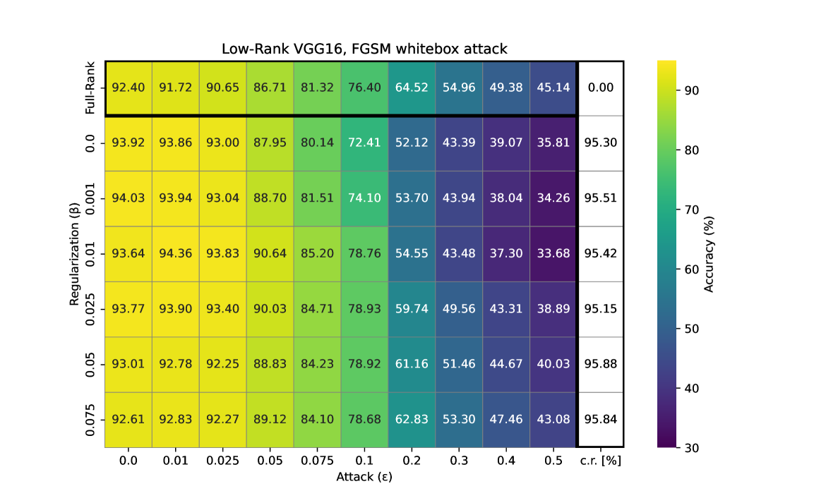
Figure 4: UCM Dataset, VGG16 clean and adversarial accuracy under the FGSM attack. Data is averaged over 10 stochastic training runs. The top row displays the full baseline network with $0\%$ c.r. and the matrix below displays the low-rank and regularized networks trained with Algorithm˜1. All numbers display the mean of $10$ randomized training runs, where the randomness stems from shuffled batches. The initial condition of all runs is given by Imagenet-1k pretrained weights. The regularized low-rank networks with $\beta=0.075$ are able to recover the adversarial robustness of the baseline training while compressed by 95.84%. Results for VGG11 and Vit32b are similar.

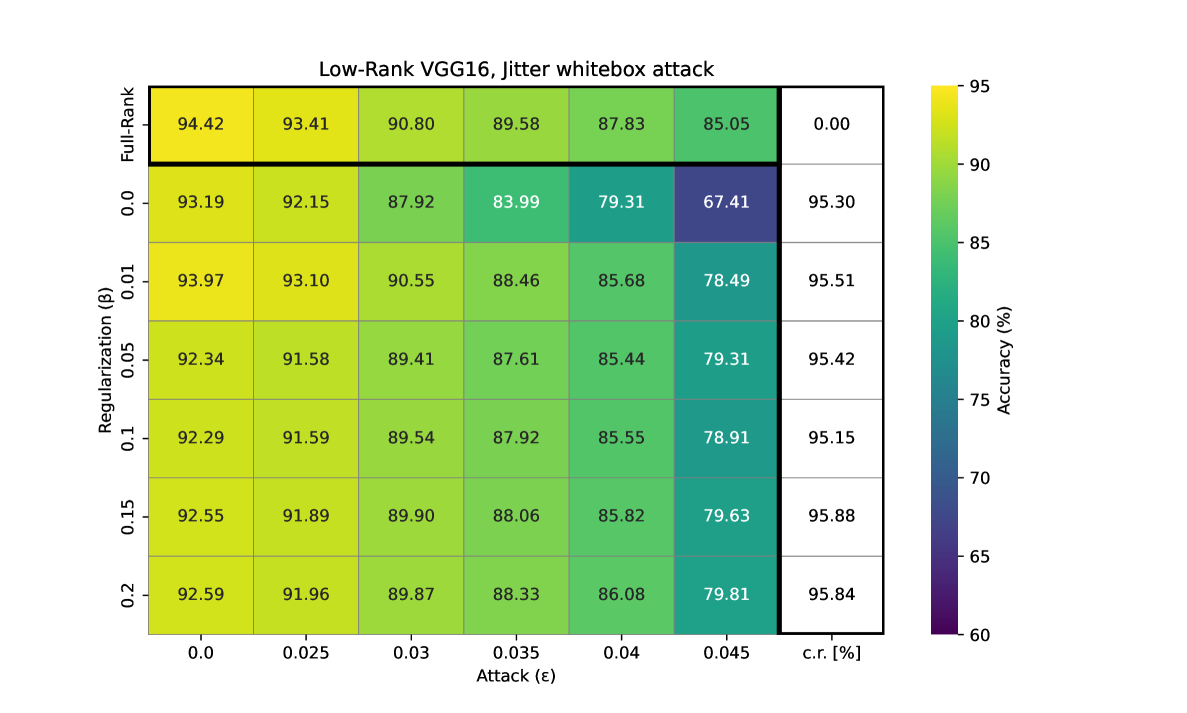
Figure 5: UCM Dataset, VGG16 clean and adversarial accuracy under the Jitter attack. Data is averaged over 10 stochastic training runs. The top row displays the full baseline network with $0\%$ c.r. and the matrix below displays the low-rank and regularized networks trained with Algorithm˜1. All numbers display the mean of $10$ randomized training runs, where the randomness stems from shuffled batches. The initial condition of all runs is given by Imagenet-1k pretrained weights. The regularized low-rank networks are able to recover most of the adversarial robustness of the baseline network. Results for VGG11 and Vit32b are similar.

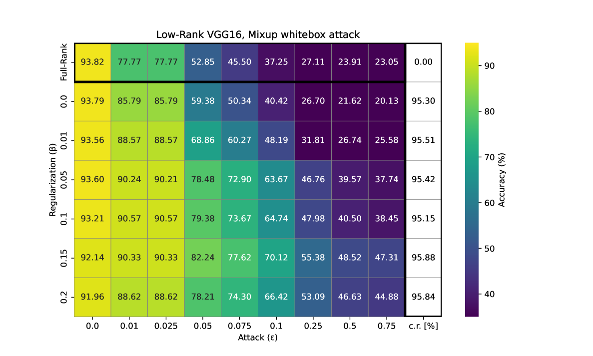
Figure 6: VGG16

Figure 7: UCM Dataset, VGG16 clean and adversarial accuracy under the Mixup attack. Data is averaged over 10 stochastic training runs. The top row displays the full baseline network with $0\%$ c.r. and the matrix below displays the low-rank and regularized networks trained with Algorithm˜1. All numbers display the mean of $10$ randomized training runs, where the randomness stems from shuffled batches. The initial condition of all runs is given by Imagenet-1k pretrained weights. The regularized low-rank networks almost double the adversarial accuracy of the baseline network at $95.84\%$ compression rate. Results for VGG11 and Vit32b are similar.

A.4 Cifar10

The Cifar10 dataset consists of 10 classes, with a total of 60000 rgb images with a resolution of $32\times 32$ pixels.

We use standard data augmentation techniques. That is, for CIFAR10, we augment the training data set by a random horizontal flip of the image, followed by a normalization using mean $[0.4914,0.4822,0.4465]$ and std. dev. $[0.2470,0.2435,0.2616]$. The test data set is only normalized. The convolutional neural neural networks used in this work are applied to the original $32\times 32$ image size. The vision transformer data-pipeline resizes the image to a resolution of $224\times 224$ pixels. The adversarial attacks for this dataset are performed on the resized images.

A.5 Computational hardware

All experiments in this paper are computed using workstation GPUs. Each training run used a single GPU. Specifically, we have used 5 NVIDIA RTX A6000, 3 NVIDIA RTX 4090, and 8 NVIDIA A-100 80G.

The estimated time for one experimental run depends mainly on the data-set size and neural network architecture. For training, generation of adversarial examples and validation testing we estimate $30$ minutes on one GPU for one run.

Appendix B Proofs

For the following proofs, let

$$(A,B)=\text{trace}(B^{\top}A)=\sum_{ij}A_{ij}B_{ij}$$

be the Frobenius inner product that induces the norm $\|A\|=\sqrt{(A,A)}$. By the cyclic property of the trace, we have

$$(AB,CD)=(B,CDA^{\top})=(C^{\top}\!AB,D).$$ (25)

for matrices $A$, $B$, $C$, and $D$ of appropriate size.

Proof of (3).

We calculate

$$\begin{split}{\mathcal{R}}(S)^{2}&=(S^{\top}\!S-\alpha_{S}^{2}I,S^{\top}\!S-\alpha_{S}^{2}I)\\ &=\|S^{\top}\!S\|^{2}-2\alpha_{S}^{2}(S^{\top}\!S,I)+\alpha_{S}^{4}(I,I)\\ &=\|S^{\top}\!S\|^{2}-\tfrac{1}{r}\|S\|^{4}\\ &=\sum_{i=1}^{r}\sigma_{i}(S^{\top}\!S)^{2}-\frac{1}{r}\bigg{(}\sum_{i=1}^{r}\sigma_{i}(S)^{2}\bigg{)}^{2}\\ &=r\bigg{(}\frac{1}{r}\sum_{i=1}^{r}\sigma_{i}(S^{\top}\!S)^{2}-\bigg{(}\frac{1}{r}\sum_{i=1}^{r}\sigma_{i}(S)^{2}\bigg{)}^{2}\bigg{)}\end{split}$$ (26)

Since $S^{\top}\!S$ is symmetric positive semi-definite, $\sigma_{i}(S^{\top}\!S)=\sigma_{i}(S)^{2}$. Applying this substitution yields (3). The proof is complete. ∎

Proof of ˜1.

Given $S\in\mathbb{R}^{r\times r}$, the Fréchet derivative for ${\mathcal{Q}}={\mathcal{R}}^{2}$ at $S$ is a linear operator $Z\to{\nabla}{\mathcal{Q}}(S)[Z]$ for $Z\in\mathbb{R}^{r\times r}$. Denote $W_{S}=S^{\top}\!S-\alpha_{S}^{2}I$ which is symmetric. Since ${\mathcal{Q}}$ is an inner product, we calculate ${\nabla}{\mathcal{Q}}(S)[Z]$ as

$$\begin{split}\tfrac{1}{2}{\nabla}{\mathcal{Q}}(S)[Z]&=(W_{S},Z^{\top}\!S+S^{\top}\!Z-\tfrac{2}{r}(S,Z)I)\\ &=(W_{S},Z^{\top}\!S)+(W_{S},S^{\top}\!Z)-\tfrac{2}{r}(S,Z)(W_{S},I)\\ &=(SW_{S}^{\top},Z)+(SW_{S},Z)-\tfrac{2}{r}(S,Z)(W_{S},I)\\ &=2(S(S^{\top}\!S-\alpha_{S}^{2}I),Z)-\tfrac{2}{r}(S,Z)(S^{\top}\!S-\alpha_{S}^{2}I,I).\end{split}$$ (27)

Note by definition of $\alpha_{S}^{2}$,

$$(S^{\top}\!S-\alpha_{S}^{2}I,I)=\|S\|^{2}-\alpha_{S}^{2}\|I\|^{2}=0.$$ (28)

Hence

$${\nabla}{\mathcal{Q}}(S)=4S(S^{\top}\!S-\alpha_{S}^{2}I).$$ (29)

Since ${\mathcal{R}}^{2}={\mathcal{Q}}$, therefore

$${\nabla}{\mathcal{R}}(S)=\tfrac{{\nabla}{\mathcal{Q}}(S)}{2{\mathcal{R}}(S)}.$$ (30)

The desired estimate follows. The proof is complete. ∎

Proof of ˜2.

From (3) and noting $\sigma_{i}(S^{\top}\!S)=\sigma_{i}(S)^{2}$, we obtain

$$\frac{1}{r}{\mathcal{R}}(S)^{2}=\frac{1}{r}\sum_{i=1}^{r}\sigma_{i}(S^{\top}\!S)^{2}-\bigg{(}\frac{1}{r}\sum_{i=1}^{r}\sigma_{i}(S^{\top}\!S)\bigg{)}^{2}.$$ (31)

From (31), $\tfrac{1}{r}{\mathcal{R}}(S)^{2}$ is the variance of the sequence $\{\sigma_{i}(S^{\top}\!S)\}_{i=1}^{r}$. The Von Szokefalvi Nagy inequality [27] bounds the variance of a finite sequence of numbers below by the range of the sequence (see [34]). Applied to (31), this yields

$$\frac{1}{r}{\mathcal{R}}(S)^{2}\geq\frac{(\sigma_{1}(S^{\top}\!S)-\sigma_{r}(S^{\top}\!S))^{2}}{2r}=\frac{(\sigma_{1}(S)^{2}-\sigma_{r}(S)^{2})^{2}}{2r}.$$ (32)

Hence

$$\sqrt{2}{\mathcal{R}}(S)\geq\sigma_{1}(S)^{2}-\sigma_{r}(S)^{2}.$$ (33)

An application of the Mean Value Theorem for logarithms (see [28, Proof of Theorem 2.2]), gives

$$\ln(\kappa(S))\leq\frac{\sigma_{1}(S)^{2}-\sigma_{r}(S)^{2}}{2\sigma_{r}(S)^{2}}.$$ (34)

Combining (33) and (34) yields

$$\ln(\kappa(S))\leq\frac{1}{\sqrt{2}\sigma_{r}(S)^{2}}{\mathcal{R}}(S),$$ (35)

which, after exponentiation, yields (4). The proof is complete. ∎

Proof of ˜3.

Since $W$ is constant, we rewrite the dynamical system $\dot{S}+\beta{\nabla}{\mathcal{R}}(S)+S=W$ as

$$\tfrac{\mathrm{d}}{\mathrm{d}t}(S-W)+\beta{\nabla}{\mathcal{R}}(S)+(S-W)=0.$$ (36)

Testing (36) by $S-W$ and rearranging yields

$$\tfrac{1}{2}\tfrac{\mathrm{d}}{\mathrm{d}t}\|S-W\|^{2}+\beta({\nabla}{\mathcal{R}}(S),S)+\|S-W\|^{2}=\beta({\nabla}{\mathcal{R}}(S),W).$$ (37)

We calculate $({\nabla}{\mathcal{R}}(S),S)$. Note

$$\begin{split}(S(S^{\top}S-\alpha_{S}^{2}I),S)&=(S^{\top}\!S-\alpha_{S}^{2}I,S^{\top}\!S)\\ &=\|S^{\top}S\|^{2}-\alpha_{S}^{2}(I,S^{\top}\!S)=\|S^{\top}\!S\|^{2}-\tfrac{1}{r}\|S\|^{4}={\mathcal{R}}(S)^{2},\end{split}$$ (38)

where the last equality is due to (26). Hence

$$({\nabla}{\mathcal{R}}(S),S)=\frac{2S(S^{\top}\!S-\alpha_{S}^{2}I,S)}{{\mathcal{R}}(S)}=2{\mathcal{R}}(S).$$ (39)

Using Hölder’s inequality, the sub-multiplicative property of $\|\cdot\|$, and Young’s inequality, we bound the right hand side of (37) by

$$\begin{split}\beta({\nabla}{\mathcal{R}}(S),W)&\leq 2\beta\frac{\|S(S^{\top}\!S-\alpha_{S}^{2}I)\|}{{\mathcal{R}}(S)}\|W\|\leq 2\beta\|S\|\|W\|\\ &\leq 2\beta(\|S-W\|\|W\|+\|W\|^{2})\leq\tfrac{1}{2}\|S-W\|^{2}+2\beta(1+2\beta)\|W\|^{2}.\end{split}$$ (40)

Applying (39) and (40) to (36) we obtain

$$\tfrac{1}{2}\tfrac{\mathrm{d}}{\mathrm{d}t}\|S-W\|^{2}+2\beta{\mathcal{R}}(S)+\tfrac{1}{2}\|S-W\|^{2}\leq 2\beta(1+2\beta)\|W\|^{2}.$$ (41)

An application of Grönwall’s inequality on $[0,t]$ yields

$$\tfrac{1}{2}\|S(t)-W\|^{2}+2\beta\int_{0}^{t}e^{\tau-t}{\mathcal{R}}(S(\tau))\,\mathrm{d}\tau=\tfrac{1}{2}e^{-t}\|S(0)-W\|^{2}+2(1-e^{-t})\beta(1+2\beta)\|W\|^{2}.$$ (42)

The proof is complete. ∎

References

- [1] P.-A. Absil and J. Malick. Projection-like retractions on matrix manifolds. SIAM Journal on Optimization, 22(1):135–158, 2012.
- [2] A. Aghajanyan, S. Gupta, and L. Zettlemoyer. Intrinsic dimensionality explains the effectiveness of language model fine-tuning. In Proceedings of the 59th Annual Meeting of the Association for Computational Linguistics and the 11th International Joint Conference on Natural Language Processing (Volume 1: Long Papers), pages 7319–7328, 2021.
- [3] C. Anil, J. Lucas, and R. Grosse. Sorting out Lipschitz function approximation. In International conference on machine learning, pages 291–301. PMLR, 2019.
- [4] N. Bansal, X. Chen, and Z. Wang. Can we gain more from orthogonality regularizations in training deep networks? Advances in Neural Information Processing Systems, 31, 2018.
- [5] G. Ceruti, J. Kusch, and C. Lubich. A rank-adaptive robust integrator for dynamical low-rank approximation. BIT Numerical Mathematics, pages 1–26, 2022.
- [6] G. Ceruti and C. Lubich. An unconventional robust integrator for dynamical low-rank approximation. BIT Numerical Mathematics, 62(1):23–44, 2022.
- [7] G. Cheng, X. Sun, K. Li, L. Guo, and J. Han. Perturbation-seeking generative adversarial networks: A defense framework for remote sensing image scene classification. IEEE Transactions on Geoscience and Remote Sensing, 60:1–11, 2022.
- [8] M. Cisse, P. Bojanowski, E. Grave, Y. Dauphin, and N. Usunier. Parseval networks: Improving robustness to adversarial examples. In D. Precup and Y. W. Teh, editors, Proceedings of the 34th International Conference on Machine Learning, volume 70 of Proceedings of Machine Learning Research, pages 854–863. PMLR, 06–11 Aug 2017.
- [9] M. Cisse, P. Bojanowski, E. Grave, Y. Dauphin, and N. Usunier. Parseval networks: Improving robustness to adversarial examples. In International Conference on Learning Representations (ICLR), 2017.
- [10] W. Czaja, N. Fendley, M. Pekala, C. Ratto, and I.-J. Wang. Adversarial examples in remote sensing. In Proceedings of the 26th ACM SIGSPATIAL International Conference on Advances in Geographic Information Systems, SIGSPATIAL ’18, page 408–411, New York, NY, USA, 2018. Association for Computing Machinery.
- [11] E. L. Denton, W. Zaremba, J. Bruna, Y. LeCun, and R. Fergus. Exploiting linear structure within convolutional networks for efficient evaluation. Advances in neural information processing systems, 27, 2014.
- [12] Y. Guo, A. Yao, and Y. Chen. Dynamic network surgery for efficient dnns. Advances in neural information processing systems, 29, 2016.
- [13] M. Hein and M. Andriushchenko. Formal guarantees on the robustness of a classifier against adversarial manipulation. Advances in neural information processing systems, 30, 2017.
- [14] A. Hnatiuk, J. Kusch, L. Kusch, N. R. Gauger, and A. Walther. Stochastic aspects of dynamical low-rank approximation in the context of machine learning. Optimization Online, 2024.
- [15] E. J. Hu, Y. Shen, P. Wallis, Z. Allen-Zhu, Y. Li, S. Wang, L. Wang, and W. Chen. Lora: Low-rank adaptation of large language models. arXiv preprint arXiv:2106.09685, 2021.
- [16] O. Koch and C. Lubich. Dynamical low-rank approximation. SIAM Journal on Matrix Analysis and Applications, 29(2):434–454, 2007.
- [17] A. Kurakin, I. J. Goodfellow, and S. Bengio. Adversarial machine learning at scale. In International Conference on Learning Representations, 2017.
- [18] J. Kusch, S. Schotthöfer, and A. Walter. An augmented backward-corrected projector splitting integrator for dynamical low-rank training. arXiv preprint arXiv:2502.03006, 2025.
- [19] V. Lebedev, Y. Ganin, M. Rakhuba, I. Oseledets, and V. Lempitsky. Speeding-up convolutional neural networks using fine-tuned CP-decomposition. In International Conference on Learning Representations, 2015.
- [20] H. Lee, S. Han, and J. Lee. Generative adversarial trainer: Defense to adversarial perturbations with GAN. arXiv preprint arXiv:1705.03387, 2017.
- [21] J. Li, F. Li, and S. Todorovic. Efficient Riemannian optimization on the Stiefel manifold via the Cayley transform. In International Conference on Learning Representations, 2020.
- [22] J. Lin, C. Song, K. He, L. Wang, and J. E. Hopcroft. Nesterov accelerated gradient and scale invariance for adversarial attacks. In International Conference on Learning Representations, 2020.
- [23] X. Liu, Y. Li, C. Wu, and C.-J. Hsieh. Adv-BNN: Improved adversarial defense through robust Bayesian neural network. In International Conference on Learning Representations, 2010.
- [24] C. Lubich and I. V. Oseledets. A projector-splitting integrator for dynamical low-rank approximation. BIT Numerical Mathematics, 54(1):171–188, 2014.
- [25] Y. Mao, K. Huang, C. Guan, G. Bao, F. Mo, and J. Xu. DoRA: Enhancing parameter-efficient fine-tuning with dynamic rank distribution. In L.-W. Ku, A. Martins, and V. Srikumar, editors, Proceedings of the 62nd Annual Meeting of the Association for Computational Linguistics (Volume 1: Long Papers), pages 11662–11675, Bangkok, Thailand, Aug. 2024. Association for Computational Linguistics.
- [26] T. Miyato, T. Kataoka, M. Koyama, and Y. Yoshida. Spectral normalization for generative adversarial networks. In International Conference on Learning Representations, 2018.
- [27] J. Nagy. Über algebraische gleichungen mit lauter reellen wurzeln. Jahresbericht der Deutschen Mathematiker-Vereinigung, 27:37–43, 1918.
- [28] R. Nenov, D. Haider, and P. Balazs. (Almost) smooth sailing: Towards numerical stability of neural networks through differentiable regularization of the condition number, 2024.
- [29] D. Savostianova, E. Zangrando, G. Ceruti, and F. Tudisco. Robust low-rank training via approximate orthonormal constraints. Advances in Neural Information Processing Systems, 36:66064–66083, 2023.
- [30] S. Schotthöfer and M. P. Laiu. Federated dynamical low-rank training with global loss convergence guarantees. arXiv preprint arXiv:2406.17887, 2024.
- [31] S. Schotthöfer, E. Zangrando, G. Ceruti, F. Tudisco, and J. Kusch. GeoLoRA: Geometric integration for parameter efficient fine-tuning. In The Thirteenth International Conference on Learning Representations, 2025.
- [32] S. Schotthöfer, E. Zangrando, K. Jonas, G. Ceruti, and F. Tudisco. Low-rank lottery tickets: finding efficient low-rank neural networks via matrix differential equations. In Advances in Neural Information Processessing Systems, 2022.
- [33] L. Schwinn, R. Raab, A. Nguyen, D. Zanca, and B. Eskofier. Exploring misclassifications of robust neural networks to enhance adversarial attacks, 2021.
- [34] R. Sharma, M. Gupta, and G. Kapoor. Some better bounds on the variance with applications. Journal of Mathematical Inequalities, 4(3):355–363, 2010.
- [35] S. P. Singh, G. Bachmann, and T. Hofmann. Analytic insights into structure and rank of neural network Hessian maps. In Advances in Neural Information Processing Systems, volume 34, 2021.
- [36] Y. Su, G. Zhang, S. Mei, J. Lian, Y. Wang, and S. Wan. Reconstruction-assisted and distance-optimized adversarial training: A defense framework for remote sensing scene classification. IEEE Transactions on Geoscience and Remote Sensing, 61:1–13, 2023.
- [37] F. Tramèr, A. Kurakin, N. Papernot, I. Goodfellow, D. Boneh, and P. McDaniel. Ensemble adversarial training: Attacks and defenses, 2020.
- [38] L. N. Trefethen and D. Bau. Numerical Linear Algebra. SIAM, Philadelphia, PA, 1997.
- [39] M. Valipour, M. Rezagholizadeh, I. Kobyzev, and A. Ghodsi. Dylora: Parameter efficient tuning of pre-trained models using dynamic search-free low-rank adaptation, 2023.
- [40] H. Wang, S. Agarwal, and D. Papailiopoulos. Pufferfish: Communication-efficient models at no extra cost. Proceedings of Machine Learning and Systems, 3:365–386, 2021.
- [41] D. Xie, J. Xiong, and S. Pu. All you need is beyond a good init: Exploring better solution for training extremely deep convolutional neural networks with orthonormality and modulation. In Proceedings of the IEEE Conference on Computer Vision and Pattern Recognition, pages 6176–6185, 2017.
- [42] Y. Xu and P. Ghamisi. Universal adversarial examples in remote sensing: Methodology and benchmark. IEEE Transactions on Geoscience and Remote Sensing, 60:1–15, 2022.
- [43] H. Yang, M. Tang, W. Wen, F. Yan, D. Hu, A. Li, H. Li, and Y. Chen. Learning low-rank deep neural networks via singular vector orthogonality regularization and singular value sparsification, 2020.
- [44] Y. Yang and S. Newsam. Bag-of-visual-words and spatial extensions for land-use classification. In Proceedings of the 18th SIGSPATIAL International Conference on Advances in Geographic Information Systems, GIS ’10, page 270–279, New York, NY, USA, 2010. Association for Computing Machinery.
- [45] E. Zangrando, S. Schotthöfer, G. Ceruti, J. Kusch, and F. Tudisco. Geometry-aware training of factorized layers in tensor tucker format. In A. Globerson, L. Mackey, D. Belgrave, A. Fan, U. Paquet, J. Tomczak, and C. Zhang, editors, Advances in Neural Information Processing Systems, volume 37, pages 129743–129773. Curran Associates, Inc., 2024.
- [46] E. Zangrando, S. Schotthöfer, G. Ceruti, J. Kusch, and F. Tudisco. Rank-adaptive spectral pruning of convolutional layers during training. In Advances in Neural Information Processing Systems, 2024.
- [47] H. Zhang, Y. Yu, J. Jiao, E. Xing, L. El Ghaoui, and M. Jordan. Theoretically principled trade-off between robustness and accuracy. In International conference on machine learning, pages 7472–7482. PMLR, 2019.
- [48] Q. Zhang, M. Chen, A. Bukharin, P. He, Y. Cheng, W. Chen, and T. Zhao. AdaLoRA: Adaptive budget allocation for parameter-efficient fine-tuning. In The Eleventh International Conference on Learning Representations, 2023.
- [49] J. Zhao, Z. Zhang, B. Chen, Z. Wang, A. Anandkumar, and Y. Tian. GaLore: Memory-efficient LLM training by gradient low-rank projection. In International Conference on Machine Learning, pages 61121–61143. PMLR, 2024.