RDD: Robust Feature Detector and Descriptor using Deformable Transformer

Abstract

As a core step in structure-from-motion and SLAM, robust feature detection and description under challenging scenarios such as significant viewpoint changes remain unresolved despite their ubiquity. While recent works have identified the importance of local features in modeling geometric transformations, these methods fail to learn the visual cues present in long-range relationships. We present Robust Deformable Detector (RDD), a novel and robust keypoint detector/descriptor leveraging the deformable transformer, which captures global context and geometric invariance through deformable self-attention mechanisms. Specifically, we observed that deformable attention focuses on key locations, effectively reducing the search space complexity and modeling the geometric invariance. Furthermore, we collected an Air-to-Ground dataset for training in addition to the standard MegaDepth dataset. Our proposed method outperforms all state-of-the-art keypoint detection/description methods in sparse matching tasks and is also capable of semi-dense matching. To ensure comprehensive evaluation, we introduce two challenging benchmarks: one emphasizing large viewpoint and scale variations, and the other being an Air-to-Ground benchmark — an evaluation setting that has recently gaining popularity for 3D reconstruction across different altitudes. Project page: https://xtcpete.github.io/rdd/.

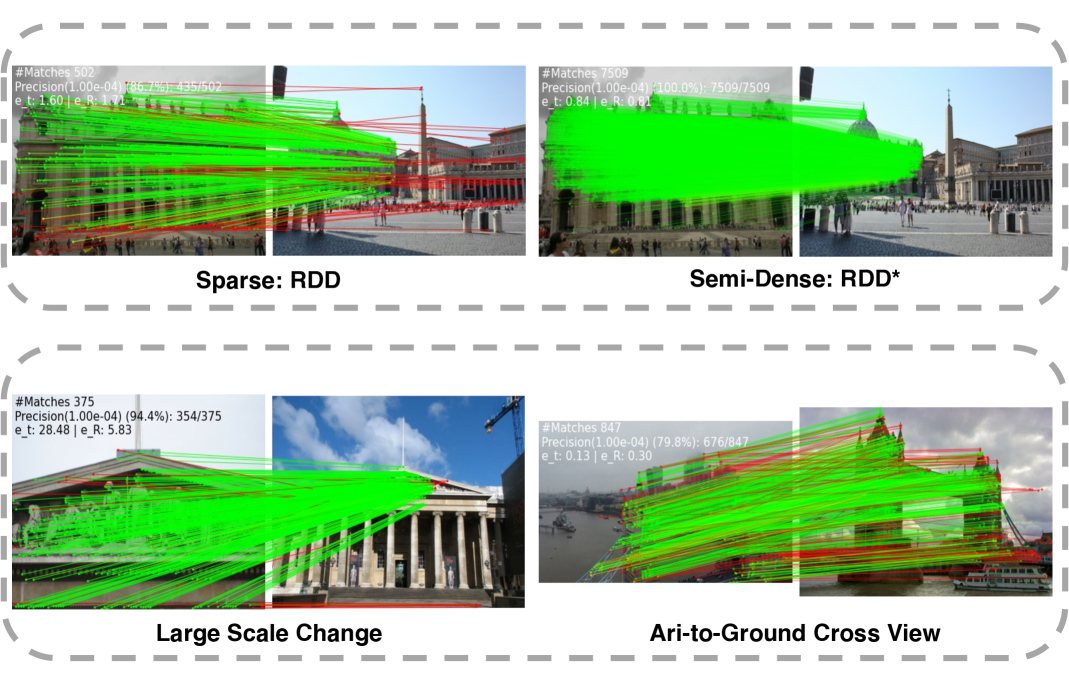
Figure 1: Our proposed method effectively performs both sparse and semi-dense feature matching, referred to as RDD and RDD*, respectively, as shown in the top section. RDD demonstrates its ability to extract accurate keypoints and robust descriptors, enabling reliable matching even under significant scale and viewpoint variations, as illustrated in the bottom section.

1 Introduction

Keypoint detection and description are central to numerous 3D computer vision tasks, including structure-from-motion (SfM), visual localization, and simultaneous localization and mapping (SLAM). These tasks depend on reliable keypoints and descriptors to establish accurate tracks, which are crucial for downstream algorithms to interpret spatial relationships—a requirement in fields from robotics to augmented reality [20]. When applied to real-world tasks, these systems face challenges such as significant viewpoint shifts, lighting variations, and scale changes.

Historically, feature detection and description methods relied on rule-based techniques such as SIFT , SURF, and ORB [25, 3, 35]. However, these methods oftenf struggled with the aforementioned challenges. To better address these issues, recent works [6, 13, 41, 46] leverage deep neural networks based on data-driven approaches which often extract more robust and discriminative descriptors than the rule-based ones. Despite the enhanced robustness that learning-based methods have, they often rely on regular convolutions to encode images [6, 41, 13, 32, 46], which ignore the geometric invariance and long-distance awareness critical for robust description under challenging conditions. Subsequently, [28, 45, 26] have partially addressed geometric invariance by estimating the scale and orientation of keypoint descriptors to model affine transformations. ALIKED [47] and ASLFeat [28] advanced this approach by using deformable convolutions capable of modeling any geometric transformations. However, these methods are limited to modeling transformations within local windows; features learned with the localized kernels of convolution operators fall short of learning important visual cues that depend on long-range relationships (e.g. vanishing lines).

In this paper, we focus on feature detection and description in challenging scenarios that haven’t been effectively addressed in prior works – specifically, extracting reliable and discriminative keypoints and descriptors across images with large camera baselines, significant illumination variations, and scale changes. We therefore propose RDD: a novel two-branch architecture for keypoint detection and description that can model both geometric invariance and global context at the same time. In particular, we design two dedicated network branches: a fully convolutional architecture to perform keypoint detection and a transformer-based architecture for extracting descriptors: the objectives of keypoint detection and description have previously been found not to align perfectly [21]. We observe that the convolutional neural network excels in detecting sub-pixel keypoints thanks to its expressiveness, whereas a transformer-based architecture is particularly suited for learning features that captures global context and possess geometric invariance through its self-attention mechanism [42, 7]. However, as self-attention layers attend to all spatial locations in the image, they significantly increase computational overhead and may reduce descriptor discriminability. To address this, we have adopted the deformable attention [48] for keypoint description, allowing our designed network to selectively focus on key locations, which greatly reduces time complexity while maintaining the capability to learn geometric invariance and global context.

The two-branch architecture of RDD allows specialized architectures to learn keypoint detection and description independently. Our experiments have found that such design choice accelerates convergence and leads to better overall performance, as proven in Sec. 4.4. Overall, RDD is designed to be robust, achieving competitive performance on challenging imagery and also capable of semi-dense matching Fig. 1. This enhanced capability improves accuracy and stability in 3D vision applications, such as structure-from-motion (SfM) [4] and relative camera pose estimation under difficult imaging conditions. Our approach outperforms current state-of-the-art methods for keypoint detection and description on standard benchmarks, including MegaDepth-1500 [8], HPatches [1], and Aachen-Day-Night [38], across various tasks. However, to the best of our knowledge, no existing benchmarks accurately capture the aftermentioned challenging scenarios. To further validate the robustness of our method and provide a more comprehensive evaluation, we have collected and derived two additional benchmark datasets. The main contributions of our work are:

• A novel two branch architecture that utilizes a convolutional neural network for detecting accurate keypoints and transformer based network to extract robust descriptors under challenging scenarios, all while maintaining efficient runtime performance.

• An innovative refinement module for semi-dense matching, improving matching accuracy and density.

• Dataset contribution: MegaDepth-View, derived from MegaDepth [22], specifically focuses on challenging image pairs with large viewpoint and scale variations. Air-to-Ground dataset provides diverse aerial and ground cross view imagery for training and evaluation, enhancing robustness and performance and providing a new evaluation setting.

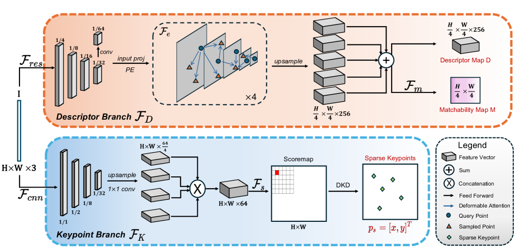
Figure 2: An overview of our network architecture. Descriptor Branch $\mathcal{F}_{D}$ and Keypoint Branch $\mathcal{F}_{K}$ process an input image $I\in\mathbb{R}^{H\times W\times 3}$ independently. Descriptor Branch: 4 layers of multiscale feature maps $\{\mathbf{x}_{res}^{l}\}_{l=1}^{L}$ are extracted by passing $I$ through ResNet-50 [15] $\mathcal{F}_{res}$. Additional feature map at scale of $1/64$ is added by applying a simple CNN on the last feature map and then they are feed to a transformer encoder $\mathcal{F}_{e}$ with positional embeddings [42]. We up-sample all feature maps output by $\mathcal{F}_{e}$ to size $H/k\times W/k$ where $k=4$ is the patch size. Feature maps are then summed together to generate the dense descriptor map $D$. A classification head $\mathcal{F}_{m}$ is applied to the descriptor map to estimate a matchability map $M$. Keypoint Branch: $I$ passes through a lightweight CNN with residual connection [15] $\mathcal{F}_{cnn}$ to capture multi-scale features $\{\mathbf{x}_{cnn}^{l}\}_{l=1}^{L}$. Features are then up-sampled to size $H\times W$ and concatenated to generate a feature map of $H\times W\times 64$. A score map $S$ is estimated by a classification head $\mathcal{F}_{s}$. Final sub-pixel keypoints are detected using DKD [46].

2 Related Work

2.1 Geometric Invariant Descriptors

In geometric invariance modeling, previous methods have primarily focused on two key aspects: scale and orientation. In traditional hand-crafted methods, SIFT [25] estimates a keypoint’s scale and orientation by analyzing histograms of image gradients and subsequently extracts and normalizes image patches around the keypoint to construct scale- and orientation-invariant descriptors. Similarly, ORB [35] computes orientation based on the keypoint’s center of mass, followed by rotation of the image patches to ensure orientation invariance.

Learning-based methods approach geometric invariance through two primary strategies. The majority of these methods [6, 41, 8, 33, 13, 32] relies heavily on data augmentation techniques to achieve scale and orientation invariance. On the other hand, some learning-based approaches explicitly model scale and orientation. For instance, LIFT [45] mimics SIFT [25] by detecting keypoints, estimating their orientation, and extracting descriptors with different neural networks. Other methods, such as AffNet [30] and LF-Net [31], predict affine transformation parameters and apply these transformations via Spatial Transformer Networks [18] to produce affine-invariant descriptors. These methods generally assume a predefined geometric transformation, typically affine transformations. More recent advancements, such as ASLFeat [28] and ALIKED [47], employ deformable convolutions to directly extract geometric-invariant features, offering a more flexible and adaptive approach to handling geometric variations.

Inspired by the use of deformable convolutions in feature description, the proposed network RDD employs deformable attention to extract geometric invariant features that are not restricted by local windows.

2.2 Decoupling Keypoint and Descriptor Learning

In traditional handcrafted methods for feature detection and description, such as SIFT [25] and ORB [35], the detection and description processes are performed independently. This decoupled approach was also common in early learning-based methods [2, 29], where keypoint detection and description were treated as separate tasks. However, later works [8, 6, 13, 33] proposed an end-to-end framework, jointly optimizing keypoint detection and descriptor extraction. This joint learning approach ensures that the detected keypoints and their descriptors complement each other. Despite the advantages,  [21] highlighted a potential drawback of joint training, observing that poorly learned descriptors could negatively impact keypoint detection quality. Subsequently, DeDoDe[10] demonstrated that decoupling keypoint detection and description into two independent networks can significantly improve performance. Similarly, XFeat [32] showed that using task-specific networks provides a better balance between efficiency and accuracy. Inspired by these recent insights, RDD consists of two separate branches for independent keypoint detection and description. We also formulate a training strategy that optimize the descriptor branch first and then the keypoint branch. This design enables both sparse and dense matching and ensures optimized performance across various scenarios.

2.3 Efficient Attention Mechanisms

The quadratic complexity of multi-head attention [42] leads to long training schedules and limited spatial resolution for tractability. For 2D images, LR-Net [16] proposed a local relation layer, computing attention in a fixed local window. Linear Transformer [19] proposes to reduce the computation complexity of vanilla attention to linear complexity by substituting the exponential kernel with an alternative kernel function. Deformable attention [48] further allows the attention window to depend on the query features. With a linear projection predicting a deformable set of displacements from the center and their weight, each pixel in the feature map may attend to a fixed number of pixels of arbitrary distance. Deformable attention [48] is well-suited for our objectives, enabling efficient learning of global context, making it a fitting choice for our approach.

3 Methods

Our method extracts descriptors and keypoints separately using a descriptor branch and a keypoint branch, as shown in Fig. 2. For an input image $I\in\mathbb{R}^{H\times W\times 3}$, the descriptor branch first extracts multi-scale feature maps $\{x_{res}^{l}\}_{l=1}^{L}$ from $I$ using ResNet-50 [15], denoted as $\mathcal{F}_{res}$, and then estimates a descriptor map $D\in\mathbb{R}^{H/k\times W/k}$ through a deformable transformer encoder [48], denoted as $\mathcal{F}_{e}$, where $k=4$ is the patch size. The matchability map $M\in\mathbb{R}^{H/k\times W/k}$ is then estimated from $D$ with a classification head $\mathcal{F}_{m}$. The keypoint branch $\mathcal{F}_{K}$ estimates a scoremap $S\in\mathbb{R}^{H\times W}$ by passing image $I$ through a lightweight CNN with residual connection [15] $\mathcal{F}_{cnn}$ and a classification head $\mathcal{F}_{s}$, then sub-pixel keypoints $p_{s}=[x,y]^{T}$ are detected with differentiable keypoint detection (DKD) [46].

The detected keypoints are used to sample their corresponding descriptors $d\in\mathbb{R}^{256}$ from $D$. In Sec. 3.1, we provide an overview of DKD [46] and deformable attention [48]. In Sec. 3.2, we introduce the network architecture. In Sec. 3.3, we discuss how sparse and dense matching are obtained. Finally, the training details and loss functions are presented in Sec. 3.4.

3.1 Preliminaries

3.1.1 Differentiable Keypoint Detection

Given the scoremap $S$, DKD detects sub-pixel keypoint locations through partially differentiable operations. First, local maximum scoremap $S_{nms}$ is obtained by non-maximum suppression in local $N\times N$ windows. Pixel-level keypoints $p_{nms}=[x^{\prime},y^{\prime}]^{T}$ are then extracted by applying a threshold to $S_{nms}$. DKD then selects all scores $s(i,j)$ in the $N\times N$ windows centered on $p_{nms}$ from $S$ and estimates a sub-pixel-level offset through following steps:

$s(i,j)$ are first normalized with softmax:

$$s^{\prime}(i,j)=\mathbf{softmax}\left(\frac{s(i,j)-s_{max}}{t_{det}}\right),$$ (1)

where $t_{det}$ is the temperature. Then $s^{\prime}(i,j)$ represents the probability of $[i,j]^{T}$ to be a keypoint within the local window. Thus, the expected position of the keypoint in the local window can be given by integral regression [40, 14]:

$$[\hat{i},\hat{j}]_{soft}^{T}=\sum_{0\leq i,j<N}s^{\prime}(i,j)[i,j]^{T}.$$ (2)

The final estimated sub-pixel-level keypoint is

$$\boldsymbol{p_{s}}=[x,y]^{T}=[x^{\prime},y^{\prime}]^{T}+[\hat{i},\hat{j}]_{soft}^{T}.$$ (3)

3.1.2 Deformable Attention

Given a feature map $\mathbf{x}\in\{\mathbf{x}_{res}^{l}\}_{l=1}^{L}$, deformable attention selects a small set of sample keys $\mathbf{p}_{q}$ corresponding to the query index $q$ and its feature vectors $\mathbf{z}_{q}$. The deformable attention feature $\mathbf{x}_{d}$ is calculated by

$$\mathbf{x}_{d}(\mathbf{z}_{q},\mathbf{p}_{q},\mathbf{x})=\sum_{m=1}^{M}\mathbf{W}_{m}A_{mq},\vskip-10.00002pt$$ (4)

where

$$A_{mq}=\sum_{k=1}^{K}A_{mqk}\cdot\mathbf{W}^{\prime}_{m}\mathbf{x}(\mathbf{p}_{q}+\Delta\mathbf{p}_{mqk}),\vskip-5.0pt$$ (5)

$m$ indexes the attention head, $k$ indexes the sampled keys, and $K$ is the total number of sampled keys. $\mathbf{W}$ and $\mathbf{W}^{\prime}$ are learnable weights. $\Delta\mathbf{p}_{mqk}$ and $A_{mqk}$ denote the sampling offset and attention weight of the $k$-th sampling point in the $m$-th attention head, where the sampling points are inferred by a linear layer.

Most of recent keypoint detection and description frameworks [10, 32, 46, 47] benefit from the use of multi-scale feature maps to capture fine details and broader spatial context. Deformable attention naturally extends to multi-scale feature maps [48], enabling the network to effectively adapt to features at different scales. Similar to Eq. 4, multi-scale deformable attention feature $\mathbf{x}_{msd}$ can be calculated similar to Eq. 4 and Eq. 7

$$\mathbf{x}_{msd}(\mathbf{z}_{q},\mathbf{p}_{q},\{\mathbf{x}^{l}\}_{l=1}^{L})=\sum_{m=1}^{M}\mathbf{W}_{m}A^{\prime}_{mq},\vskip-10.00002pt$$ (6)

where

$$A^{\prime}_{mq}=\big{[}\sum_{l=1}^{L}\sum_{k=1}^{K}A_{mlqk}\cdot\mathbf{W}^{\prime}_{m}\mathbf{x}_{l}(f_{s}(\hat{p_{q}})+\Delta\mathbf{p}_{mlqk})\big{]}.$$ (7)

Here, $\hat{p_{q}}\in[0,1]^{2}$ is the normalized coordinates and function $f_{s}$ re-scales it to match the scale of input feature map of the $l$-th level.

3.2 Network Architecture

Descriptor Branch

The descriptor branch $\mathcal{F}_{D}$ extracts a dense feature map $D\in\mathbb{R}^{H/4\times W/4\times 256}$ and a matchability map $M$, which models that probability of a given feature vector can be matched.

Using a ResNet-50 [15] as the CNN backbone, $\mathcal{F}_{res}$ extracts feature maps at 4 scales, each with resolutions of $1/4,1/8,1/16,1/32$ of the original image. An additional feature map at scale of $1/64$ is then included by applying a CNN on the last feature map. These features are positionally encoded and fed into $\mathcal{F}_{e}$ with multi-scale deformable attention [48], enabling the network to dynamically attend to relevant spatial locations across multiple scales. We use 4 encoder layers each with 8 attention heads and each head samples 8 points. The entire process of the Descriptor Branch is illustrated in Fig. 2.

Keypoint Branch

The keypoint branch is dedicated solely to detecting accurate keypoints without being influenced by descriptor estimation. $\mathcal{F}_{cnn}$ extracts feature maps at 4 different resolutions, each with a resolution of $1/1,1/2,1/8,$ and $1/32$ of the original image and feature dimension of 32. These features are subsequently upsampled to match the original image resolution and concatenated to produce a feature map of size $H\times W\times 128$. Then $\mathcal{F}_{s}$ is used to estimate the scoremap. DKD [46] is applied on the scoremap to perform non-maximum suppression and detect the sub-pixel-accurate keypoints.  Fig. 2 depicts the entire process of the Keypoint Branch.

3.3 Feature Matching

In this section, we describe how sparse matches and dense matches are obtained for a given image pair $I^{1}$ and $I^{2}$. Our network outputs sparse keypoints $p_{s}^{1,2}$, descriptor maps $D^{1,2}$, and matchability maps $M^{1,2}$ all in a single forward pass. We bilinearly upsample $D^{1,2}$ to match the original resolution of $I^{1}$ and $I^{2}$. Descriptors $d^{1,2}$ are then sampled from $D^{1,2}$ using $p_{s}^{1,2}$.

Sparse Matching

Dual-Softmax operator [34, 41] is used to establish correspondences between two descriptors $d^{1,2}$. The score matrix $S$ between the descriptors is first calculated by $S\left(i,j\right)=\frac{1}{\tau}\cdot\langle\ d^{1},d^{2}\rangle$, where $\tau$ is the temperature. We can now apply softmax on both dimensions of $S$ to obtain the probability of soft mutual nearest neighbor (MNN) matching. The matching probability matrix $P$ is obtained by:

$$P(i,j)=\operatorname{softmax}\left(S\left(i,\cdot\right)\right)_{j}\cdot\operatorname{softmax}\left(S\left(\cdot,j\right)\right)_{i}.$$ (8)

Based on the confidence matrix $P$, we select matches $m_{s}$ with confidence higher than a threshold(0.01) to further enforce the mutual nearest neighbor criteria, which filters possible outlier matches.

Semi-Dense Matching

Recent works [39, 5, 17, 43] demonstrated the benefits of semi-dense feature matching by improving coverage and number of inliers. We propose a novel dense matching module that produces accurate and geometry consistent dense matches.

Given images $I^{1}$ and $I^{2}$, our method can control the memory and computation usage by only selecting the top-K coarse keypoints $p_{c}^{1,2}$ according to their matchability score $M^{1,2}$. Then we can obtain the coarse matches $m_{c}$ using equation Eq. 8, similar to how we obtain the sparse matches $m_{s}$. These matches are naturally coarse matches and require refinement for sub-pixel level accuracy as $M$’s resolution is only $1/4$ of the original resolution. Unlike existing methods [39, 5] that crop fine level features around coarse matches in $I^{1}$ and $I^{2}$ and then predict offset in $I^{2}$, our work proposes a simple, efficient, and accurate module for semi-dense feature matching, inspired by [4] that utilizes sparse correspondences in guiding semi-dense feature matching.

Differing from [4], which iteratively reassigns the coarse matches of detector-free methods, we adopt a similar idea to refine coarse matches to fine matches. With $m_{s}$ obtained from sparse matching, we use the eight-point method to estimate a fundamental matrix $F$ that relates corresponding points between $I^{1}$ and $I^{2}$. We keep $p_{c}^{1}$ unchanged and refine $p_{c}^{2}$ by solving offsets ($\Delta x,\Delta y$) that satisfy the epipolar constraint defined by $F$. First, we convert $p_{c}^{1}$ to homogeneous coordinates $p_{h}^{1}$. Then, epipolar lines $L$ in $I^{2}$ for $p_{h}^{1}$ is computed by

$$L={F}\cdot{p_{h}^{1}},$$ (9)

where each line is represented by coefficients $a,b$ and $c$. Offsets ($\Delta x,\Delta y$) are then calculated for each point in $p_{c}^{2}$ by solving the linear equation

$$a\cdot(x+\Delta x)+b\cdot(y+\Delta y)+c=0$$ (10)

to enforce the epipolar constraint. Then we can get offsets

$$\Delta x=\frac{b(bx-ay)-ac}{a^{2}+b^{2}+\epsilon}-x,\quad\Delta y=\frac{a(ay-bx)-bc}{a^{2}+b^{2}+\epsilon}-y,$$ (11)

where $(x,y)$ are the pixel coordinates of $p_{c}^{2}$. We finally filter out points with offsets that are larger than the patch size (4) because they are moved outside the matched patch and likely outliers. We then obtain refined dense matches $m_{c}$ by $(x+\Delta x,y+\Delta y)$. In Sec. 4.4, we show that without this refinement module, the performance of dense matching degrades significantly.

3.4 Implementation Details

We train RDD with pseudo ground truth correspondences from the MegaDepth dataset [22] and our Air-to-Ground dataset. We collect data from Internet drone videos and ground images of different famous landmarks, more details can be found in the supplementary. Following [39, 37], we use poses and depths to establish pixel correspondences. For every given image pair $(I^{1},I^{2})$ with $N$ matching pixels, $m_{gt}\in R^{N\times 4}$ is defined such that the first two columns are the pixel coordinates of points in $I^{1}$ and the last two columns are those in $I^{2}$ obtained through a warping function $f_{warp}$. We train the descriptor branch and the keypoint branch separately.

Training Descriptor Branch

To supervise the local feature descriptors, we apply focal loss [23] to focus on challenging examples and reduce the influence of easily classified matches. Given descriptor maps $D^{1}$ and $D^{2}$, we sample descriptor sets $d_{gt}^{1}$ and $d_{gt}^{2}$ based on the ground truth matchability $m_{gt}/k$, where $k$ is the patch size. The $i$-th rows, $d_{gt}^{1}(i)$ and $d_{gt}^{2}(i)$, represent descriptors corresponding to the same points in the images $I^{1}$ and $I^{2}$, respectively. Using these descriptors, we compute a probability matrix $P$ as described in Eq. 8. Our supervision targets positive correspondences only, represented by the diagonal elements $P_{(i,i)}$ of $P$. By enforcing $P_{(i,i)}$ to be close to 1, we calculate the focal loss $\mathcal{L}_{focal}$ as follows:

$$\mathcal{L}_{focal}=-\alpha\cdot(1-P_{(i,i)})^{\gamma}\cdot\log(P_{(i,i)}),$$ (12)

where $\alpha=0.25$ and $\gamma=2$.

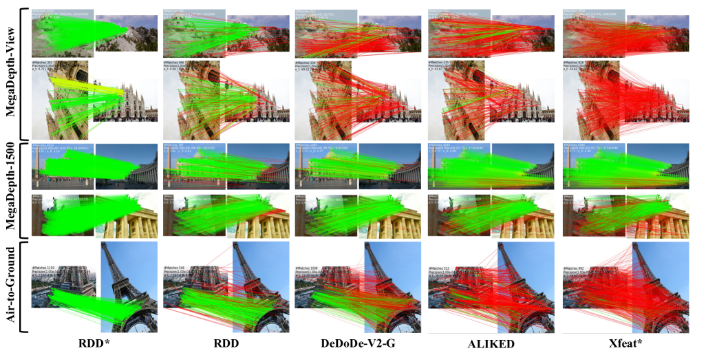
Figure 3: Qualitative Results on MegaDepth. RDD* and RDD are qualitatively compared to DeDoDe-V2-G [10, 11] ALIKED [47] and XFeat* [32]. RDD* and RDD are more robust compared DeDoDe-G* and ALIKED under challenging scenarios like large scale and viewpoint changes. The red color indicates epipolar error beyond $1\times 10^{-4}$ (in the normalized image coordinates)

To supervise the matchability map, we apply a modified focal loss that incorporates binary cross-entropy (BCE) on the matchability map $M^{1,2}$. The ground truth matchability map $M_{gt}^{1,2}$ is generated using $m_{gt}/k$. We first compute the binary cross-entropy loss $\mathcal{L}_{BCE}$ as

and then replace $P_{(i,i)}$ in Eq. 12 with $\lambda=e^{-\mathcal{L}_{BCE}}$, resulting in the matchability loss $\mathcal{L}_{matchability}$:

$$\mathcal{L}_{matchability}=-\alpha\cdot(1-\lambda)^{\gamma}\cdot\mathcal{L}_{BCE}.$$ (14)

The final loss for the descriptor branch is defined as $\mathcal{L}_{D}=\mathcal{L}_{focal}+\mathcal{L}_{matchability}$. We train the descriptor branch on the mixture of MegaDepth dataset [22] and collected Air-to-Ground dataset, with images resized to 800. The training uses a batch size of 32 image pairs and the AdamW optimizer [27]. We use a base learning rate of $1\cdot 10^{-4}$ with a step learning rate scheduler that updates the learning rate every 2000 steps after 20000 steps with $\gamma=0.5$. The descriptor branch converges after 1 day of training on 8 NVIDIA H100 GPU.

Training Keypoint Branch

We freeze the weights of descriptor branch once it converges and only supervise the keypoint branch to detect accurate and repeatable keypoints. We apply reprojection loss $\mathcal{L}_{reprojection}$, reliability loss $\mathcal{L}_{reliability}$ similar to [46, 8, 28] and dispersity peaky loss $\mathcal{L}_{peaky}$ [46] to train repeatable and reliable keypoints.

Given detected keypoint $p_{s}^{1}$ from $I^{1}$ and $p_{s}^{2}$ from $I^{2}$. We obtain the warped keypoints $p_{s}^{1\to 2}$ using $f_{warp}$ and we find their closest keypoints from $p_{s}^{2}$ with distance less than 5 pixels as matched keypoints. Then, $dist_{1\to 2}$ is the reprojection distance between the matched $p_{s}^{1}$ and $p_{s}^{2}$. We define the reprojection loss in a symmetric way:

$$\mathcal{L}_{reprojection}=\frac{1}{2}(dist_{1\to 2}+dist_{2\to 1}),$$ (15)

For keypoint $p_{s}^{1}$ and its warped keypoint $p_{s}^{1\to 2}$ with scores $s^{1}$ and $s^{1\to 2}$, and the probability map $P$ as described in Sec. 3.3, the reliability map is defined as

$$R=\exp\left(\frac{P-1}{t_{rel}}\right),$$ (16)

where $t_{rel}$ is the temperature parameter. Considering all valid $p_{s}^{1}$ and warped points $p_{s}^{1\to 2}$, we sample the reliability $r^{1}$ from $R$. The reliability loss for $p_{s}^{1}$ is then defined as

$$\mathcal{L}_{\text{reliability}}^{1}=\frac{1}{N_{1}}\sum_{p_{s}^{1},p_{s}^{1\to 2}}\frac{s^{1}\cdot s^{1\to 2}}{\sum_{p_{s}^{1},p_{s}^{1\to 2}}s^{1}\cdot s^{1\to 2}}(1-r^{1}).$$ (17)

Similarly, the total reliability loss is defined symmetrically as

$$\mathcal{L}_{\text{reliability}}=\frac{1}{2}\left(\mathcal{L}_{\text{reliability}}^{1}+\mathcal{L}_{\text{reliability}}^{2}\right).$$ (18)

Eq. 15 optimizes the scores of keypoints in local window through the soft term $[\hat{i},\hat{j}]_{soft}^{T}$ of Eq. 3, which might affect the first term $[x^{\prime},y^{\prime}]_{nms}^{T}$ of the equation. In order to align their optimization direction, we define the dispersity peak loss similiar to [46] as

$$\mathcal{L}_{peaky}=\frac{1}{N^{2}}\sum_{0\leq i,j<N}d(i,j)s^{\prime}(i,j),$$ (19)

where

$$d(i,j)=\left\{||{[i,j]-[\hat{i},\hat{j}]_{soft}}||_{p}\ |\ 0\leq i,j<N\right\},$$ (20)

$N$ is the window size and $s^{\prime}(i,j)$ are softmax scores defined in Eq. 1.

The overall loss for the keypoint branch is defined as $\mathcal{L}_{K}=\mathcal{L}_{reprojection}+\mathcal{L}_{reliability}+\mathcal{L}_{peaky}$. We use the DKD [46] with a window size of $N=5$ to detect the top 500 keypoints, and we randomly sample 500 keypoints from non-salient positions. We train the keypoint branch similarly to the descriptor branch, the keypoint branch converges after 4 hours of training on an NVIDIA H100 GPU.

4 Experiments

In this section, we demonstrate the performance of our method in Relative Pose Estimation on public benchmark datasets MegaDepth [22] and collected Air-to-Ground dataset, and in Visual Localization using Aachen Day-Night dataset [38]. All experiments are conducted on an NVIDIA H100 GPU.

4.1 Relative Pose Estimation

Dataset

Following [10, 32, 8], we use the standard MegaDepth-1500 benchmark from D2-Net [8] for outdoor pose estimation and adopt the same test split. To further validate the performance of RDD in challenging scenarios, we construct two benchmark datasets. MegaDepth-View is derived from MegaDepth [22] test scenes, focusing on pairs with large viewpoint and scale changes; additionally, we sampled 1500 pairs from our collected Air-to-Ground dataset. This benchmark is designed to validate feature matching performance for large-baseline outdoor cross-view images, which is naturally challenging because of geometric distortion and significant viewpoint changes.

Table 1: SotA comparison on the MegaDepth [22]. Results are measured in AUC (higher is better). Top 4,096 features used to all sparse matching methods. Best in bold, second best underlined.

Method	MegaDepth-1500			MegaDepth-View
	AUC			AUC
	@5°	@10°	@20°	@5°	@10°	@20°
Dense
DKM [9] CVPR’23	60.4	74.9	85.1	67.4	80.0	88.2
RoMa [12] CVPR’24	62.6	76.7	86.3	69.9	81.8	89.4
Semi-Dense
LoFTR [39] CVPR’21	52.8	69.2	81.2	50.6	65.8	77.9
ASpanFormer [5] ECCV’22	55.3	71.5	83.1	61.3	75.2	84.6
ELoFTR [44] CVPR’24	56.4	72.2	83.5	60.2	74.8	84.7
XFeat* [32] CVPR’24	38.6	56.1	70.5	23.9	37.7	51.8
RDD*	51.3	67.1	79.3	41.5	55.7	66.7
Sparse with Learned Matcher
SP [6]+SG [37] CVPR’19	49.7	67.1	80.6	51.5	65.5	76.9
SP [6]+LG [24] ICCV’23	49.9	67.0	80.1	52.4	67.3	78.5
Dedode-V2-G [10, 11]+LG [24] ICCV’23	44.1	62.1	76.5	41.9	57.1	70.0
RDD+LG [24] ICCV’23	52.3	68.9	81.8	54.2	69.3	80.3
Sparse with MNN
SuperPoint [6] CVPRW’18	24.1	40.0	54.7	7.50	13.3	21.1
DISK [41] NeurIps’20	38.5	53.7	66.6	30.4	41.9	51.6
ALIKED [47] TIM’23	41.8	56.8	69.6	30.0	41.8	53.2
XFeat [32] CVPR’24	24.0	40.1	55.8	8.82	16.5	26.8
DeDoDe-V2-G [10, 11] CVPRW’24, 3DV’24	47.2	63.9	77.5	33.1	47.6	60.2
RDD	48.2	65.2	78.3	38.3	53.1	65.6

Table 2: SotA comparison on proposed Air-to-Ground benchmark. Keypoints and descriptors are matched using dual-softmax MNN. Measured in AUC (higher is better). Best in bold, second best underlined.

Method	$@5^{\circ}$	$@10^{\circ}$	$@20^{\circ}$
SuperPoint [6] CVPRW’18	1.89	3.56	6.81
DISK [41] NeurIps’20	19.2	27.1	34.6
ALIKED [47] TIM’23	12.0	17.8	25.8
XFeat [32] CVPR’24	6.12	11.4	17.5
DeDoDe-V2-G [10, 11] CVPRW’24,3DV’24	31.5	45.3	58.3
RDD	41.4	56.0	67.8

Metrics and Comparing Methods

We report the AUC of recovered pose under threshold of (5°, 10° ,and 20°). We use RANSAC to estimate the essential matrix. We compared RDD against the state-of-the-art detector/descriptor methods [6, 41, 46, 47, 13, 10, 32] and learned matching methods [37, 24, 39, 5, 44, 9, 12] on MegaDepth [22] dataset. For Air-to-Ground dataset, RDD is compared against detector/descriptor methods. More results on Air-to-Ground data can be found in the supplementary. For all sparse methods, we use resolution whose larger dimension is set to 1,600 pixels and use top 4,096 features, while all other learned matching methods follow experiment settings mentioned in their paper.

Results

The results are presented in Tab. 1 and Tab. 2, and visually in Fig. 3. RDD demonstrates superior performance in the sparse matching setting compared to the state-of-the-art method DeDoDe-V2-G [10, 11], especially in more challenging scenarios. RDD with learned matcher LightGlue [24] also outperforms previous methods.

The results on MegaDepth-View and Air-to-Ground prove the effectiveness of our method under challenging scenarios with significant improvements over previous methods. RDD outperforms all previous feature detector/descriptor methods under large viewpoints and scale changes.

4.2 Homography Estimation

Datasets

We evaluate the quality of correspondences estimated by RDD on HPatches dataset [1] for Homography Estimation. HPatches contains 52 sequences under significant illumination changes and 56 sequences that exhibit large variation in viewpoints. We use RANSAC to robustly estimate the homography given the estimated correspondences. All images are resized such that their shorter size is equal to 480 pixels.

Table 3: Homography estimation on HPatches. All methods perform well for illumination sequences. RDD provides high quality homography estimation especially when there are significant viewpoint changes. Best in bold, second best underlined.

Method	Illumination			Viewpoint
	MHA			MHA
	@3px	@5px	@10px	@3px	@5px	@10px
SuperPoint [6] CVPRW’18	93.0	98.0	99.9	70.0	82.0	87.0
DISK [41] NeurIps’20	96.0	98.0	98.0	72.0	81.0	84.0
ALIKED [47] TIM’23	97.0	99.0	99.0	78.0	85.0	88.0
DeDoDe-G [10] 3DV’24	96.0	99.0	99.9	68.0	77.0	80.0
XFeat [32] CVPR’24	90.0	96.0	98.0	55.0	72.0	80.0
RDD	93.0	99.0	99.9	76.0	86.0	90.0

Metrics and Comparing Methods

We follow [32, 46] to estimate the mean homogeneity accuracy (MHA) with a predefined threshold of {3, 5, 7} pixels. Accuracy is computed using the average corner error in pixels by warping reference image corners onto target images using both ground truth and estimated homographies.

Results on HPatches

In Table 3, RDD shows a similar performance in illumination sequences compared to previous accurate keypoint detectors and descriptors, while outperforming most of the other methods on viewpoint changes, reinforcing the robustness of our proposed method in handling challenging cases such as large baseline pairs.

4.3 Visual Localization

Dataset

We further validate the performance of RDD on the task of visual localization, which estimates the poses of a given query image with respect to the corresponding 3D scene reconstruction. We evaluate RDD on the Aachen Day-Night dataset [38]. It focuses on localizing high-quality night-time images against a day-time 3D model. There are 14,607 images with changing conditions of weather, season, viewpoints, and day-night cycles.

Table 4: Visual Localization on Aachen day-night. RDD outperforms previous state-of-the-art methods with MNN matching for more challenging night setting. Best in bold, second best underlined.

Methods	Day		Night
	(0.25m,2°) / (0.5m,5°) / (1.0m,10°)
SuperPoint [6] CVPRW’18	87.4 / 93.2 / 97.0		77.6 / 85.7 / 95.9
DISK [41] NeurIps’20	86.9 / 95.1 / 97.8		83.7 / 89.8 / 99.0
ALIKE [46] TM’22	85.7 / 92.4 / 96.7		81.6 / 88.8 / 99.0
ALIKED [47] TIM’23	86.5 / 93.4 / 96.8		85.7 / 91.8 / 96.9
XFeat [32] CVPR’24	84.7 / 91.5 / 96.5		77.6 / 89.8 / 98.0
RDD	87.0 / 94.2 / 97.8		86.7 / 92.9 / 99.0

Table 5: Ablation study on MegaDepth. We ablate the design choices for architecture and training strategies for relative pose estimation on MegaDepth.

Variant	AUC@$5^{\circ}$
	RDD	RDD*
Full	48.2	51.3
Larger patch size $s=8$	44.6	49.4
Less sample points $N_{p_{q}}=4$	46.5	49.9
No keypoint branch	44.1	-
Joint training of two branches	42.8	46.9
No match refinement	-	41.3
Without Air-to-Ground Data	47.4	50.4

Metrics and Comparing Methods

Following [32], HLoc [36] is used to evaluate all approaches [32, 46, 6, 37, 41, 47]. We resize the images such that their longer side is equal to 1,024 pixels and sample the top 4,096 keypoints for all approaches. We use the evaluation tool provide by [38] to calculate the metrics, the AUC of estimated camera poses under threshold of $\{0.25$m$,0.5$m$,5$m$\}$ for translation errors and $\{2\degree,5\degree,10\degree\}$ for rotation errors respectively.

Results

Tab. 4 presents the results on visual localization. RDD outperforms all approaches in the challenging night setting. These results further validate the effectiveness of RDD .

4.4 Ablation

To better understand RDD, we evaluate 5 variants of RDD, with the results shown in  Tab. 5: 1) Increasing the patch size of the transformer encoder results in a significant drop in accuracy. 2) Reducing the number of sampled points per query in deformable attention degrades pose estimation accuracy. 3) Removing the keypoint branch and using upsampled matchibility map as keypoint score map with NMS negatively affect the performance. 4) Joint training of the descriptor and keypoint branches leads to a significant drop in performance, as the weights of both branches are updated when only one task fails, making it even harder for the descriptor branch to converge. 5) Simply concatenating the semi-dense matches from matchability results in worse performance. 6) Training without Air-to-Ground dataset slightly damages the performance.

5 Limitations and Conclusion

We present RDD, a robust feature detection and description framework based on deformable transformer, excelling in sparse image matching and demonstrating strong resilience to geometric transformations and varying conditions. By leveraging deformable attention, RDD efficiently extracts geometric-invariant features, enhancing accuracy and adaptability compared to traditional methods. RDD lacks explicit data augmentation during training and depends on confident priors from sparse correspondences which might lead to the failure of semi-dense matching. Training with data augmentation and improving the refinement module with visual features might boost the performance. RDD marks a significant advancement in keypoint detection and description, paving the way for impactful applications in challenging 3D vision tasks like cross-view scene modeling and visual localization.

6 Acknowledgement

Supported by the Intelligence Advanced Research Projects Activity (IARPA) via Department of Interior/ Interior Business Center (DOI/IBC) contract number 140D0423C0075. The U.S. Government is authorized to reproduce and distribute reprints for Governmental purposes notwithstanding any copyright annotation thereon. Disclaimer: The views and conclusions contained herein are those of the authors and should not be interpreted as necessarily representing the official policies or endorsements, either expressed or implied, of IARPA, DOI/IBC, or the U.S. Government. We would like to thank Yayue Chen for her help with visualization.

References

- Balntas et al. [2017] Vassileios Balntas, Karel Lenc, Andrea Vedaldi, and Krystian Mikolajczyk. Hpatches: A benchmark and evaluation of handcrafted and learned local descriptors. In CVPR, 2017.
- Barroso-Laguna et al. [2019] Axel Barroso-Laguna, Edgar Riba, Daniel Ponsa, and Krystian Mikolajczyk. Key.net: Keypoint detection by handcrafted and learned cnn filters, 2019.
- Bay et al. [2008] Herbert Bay, Andreas Ess, Tinne Tuytelaars, and Luc Van Gool. Speeded-up robust features (surf). CVIU, 110(3):346–359, 2008.
- Chen et al. [2024] Gonglin Chen, Jinsen Wu, Haiwei Chen, Wenbin Teng, Zhiyuan Gao, Andrew Feng, Rongjun Qin, and Yajie Zhao. Geometry-aware feature matching for large-scale structure from motion, 2024.
- Chen et al. [2022] Hongkai Chen, Zixin Luo, Lei Zhou, Yurun Tian, Mingmin Zhen, Tian Fang, David McKinnon, Yanghai Tsin, and Long Quan. Aspanformer: Detector-free image matching with adaptive span transformer. ECCV, 2022.
- DeTone et al. [2018] Daniel DeTone, Tomasz Malisiewicz, and Andrew Rabinovich. Superpoint: Self-supervised interest point detection and description. CVPR Workshops, pages 224–236, 2018.
- Dosovitskiy et al. [2021] Alexey Dosovitskiy, Lucas Beyer, Alexander Kolesnikov, Dirk Weissenborn, Xiaohua Zhai, Thomas Unterthiner, Mostafa Dehghani, Matthias Minderer, Georg Heigold, Sylvain Gelly, Jakob Uszkoreit, and Neil Houlsby. An image is worth 16x16 words: Transformers for image recognition at scale, 2021.
- Dusmanu et al. [2019] Mihai Dusmanu, Ignacio Rocco, Tomas Pajdla, Marc Pollefeys, Josef Sivic, Akihiko Torii, and Torsten Sattler. D2-net: A trainable cnn for joint detection and description of local features, 2019.
- Edstedt et al. [2023] Johan Edstedt, Ioannis Athanasiadis, Mårten Wadenbäck, and Michael Felsberg. DKM: Dense kernelized feature matching for geometry estimation. In IEEE Conference on Computer Vision and Pattern Recognition, 2023.
- Edstedt et al. [2024a] Johan Edstedt, Georg Bökman, Mårten Wadenbäck, and Michael Felsberg. DeDoDe: Detect, Don’t Describe — Describe, Don’t Detect for Local Feature Matching. In 2024 International Conference on 3D Vision (3DV). IEEE, 2024a.
- Edstedt et al. [2024b] Johan Edstedt, Georg Bökman, and Zhenjun Zhao. DeDoDe v2: Analyzing and Improving the DeDoDe Keypoint Detector . In IEEE/CVF Computer Society Conference on Computer Vision and Pattern Recognition Workshops (CVPRW), 2024b.
- Edstedt et al. [2024c] Johan Edstedt, Qiyu Sun, Georg Bökman, Mårten Wadenbäck, and Michael Felsberg. RoMa: Robust Dense Feature Matching. IEEE Conference on Computer Vision and Pattern Recognition, 2024c.
- Gleize et al. [2023] Pierre Gleize, Weiyao Wang, and Matt Feiszli. Silk – simple learned keypoints, 2023.
- Gu et al. [2021] Kang Gu, Lei Yang, and Anbang Yao. Removing the bias of integral pose regression. In Proceedings of the IEEE/CVF International Conference on Computer Vision, pages 11067–11076, 2021.
- He et al. [2015] Kaiming He, Xiangyu Zhang, Shaoqing Ren, and Jian Sun. Deep residual learning for image recognition, 2015.
- Hu et al. [2019] Han Hu, Zheng Zhang, Zhenda Xie, and Stephen Lin. Local relation networks for image recognition. In Proceedings of the IEEE/CVF international conference on computer vision, pages 3464–3473, 2019.
- Huang et al. [2023] Dihe Huang, Ying Chen, Yong Liu, Jianlin Liu, Shang Xu, Wenlong Wu, Yikang Ding, Fan Tang, and Chengjie Wang. Adaptive assignment for geometry aware local feature matching. CVPR, 2023.
- Jaderberg et al. [2016] Max Jaderberg, Karen Simonyan, Andrew Zisserman, and Koray Kavukcuoglu. Spatial transformer networks, 2016.
- Katharopoulos et al. [2020] Angelos Katharopoulos, Apoorv Vyas, Nikolaos Pappas, and François Fleuret. Transformers are rnns: Fast autoregressive transformers with linear attention, 2020.
- Kerbl et al. [2023] Bernhard Kerbl, Georgios Kopanas, Thomas Leimkühler, and George Drettakis. 3d gaussian splatting for real-time radiance field rendering. ACM Transactions on Graphics, 42(4), 2023.
- Li et al. [2022] Kunhong Li, Longguang Wang, Li Liu, Qing Ran, Kai Xu, and Yulan Guo. Decoupling makes weakly supervised local feature better. In Proceedings of the IEEE/CVF Conference on Computer Vision and Pattern Recognition (CVPR), pages 15838–15848, 2022.
- Li and Snavely [2018] Zhengqi Li and Noah Snavely. MegaDepth: Learning single-view depth prediction from internet photos. In CVPR, 2018.
- Lin et al. [2018] Tsung-Yi Lin, Priya Goyal, Ross Girshick, Kaiming He, and Piotr Dollár. Focal loss for dense object detection, 2018.
- Lindenberger et al. [2023] Philipp Lindenberger, Paul-Edouard Sarlin, and Marc Pollefeys. LightGlue: Local Feature Matching at Light Speed. In ICCV, 2023.
- Liu et al. [2010] Ce Liu, Jenny Yuen, and Antonio Torralba. SIFT Flow: Dense correspondence across scenes and its applications. T-PAMI, 2010.
- Liu et al. [2019] Yuan Liu, Zehong Shen, Zhixuan Lin, Sida Peng, Hujun Bao, and Xiaowei Zhou. Gift: Learning transformation-invariant dense visual descriptors via group cnns, 2019.
- Loshchilov and Hutter [2019] Ilya Loshchilov and Frank Hutter. Decoupled weight decay regularization, 2019.
- Luo et al. [2020] Zixin Luo, Lei Zhou, Xuyang Bai, Hongkai Chen, Jiahui Zhang, Yao Yao, Shiwei Li, Tian Fang, and Long Quan. Aslfeat: Learning local features of accurate shape and localization. Computer Vision and Pattern Recognition (CVPR), 2020.
- Mishchuk et al. [2018] Anastasiya Mishchuk, Dmytro Mishkin, Filip Radenovic, and Jiri Matas. Working hard to know your neighbor’s margins: Local descriptor learning loss, 2018.
- Mishkin et al. [2018] Dmytro Mishkin, Filip Radenovic, and Jiri Matas. Repeatability is not enough: Learning affine regions via discriminability, 2018.
- Ono et al. [2018] Yuki Ono, Eduard Trulls, Pascal Fua, and Kwang Moo Yi. Lf-net: Learning local features from images, 2018.
- Potje et al. [2024] Guilherme Potje, Felipe Cadar, Andre Araujo, Renato Martins, and Erickson R. Nascimento. Xfeat: Accelerated features for lightweight image matching. In 2024 IEEE / CVF Computer Vision and Pattern Recognition (CVPR), 2024.
- Revaud et al. [2019] Jerome Revaud, Philippe Weinzaepfel, César Roberto de Souza, and Martin Humenberger. R2D2: repeatable and reliable detector and descriptor. In NeurIPS, 2019.
- Rocco et al. [2018] Ignacio Rocco, Mircea Cimpoi, Relja Arandjelović, Akihiko Torii, Tomas Pajdla, and Josef Sivic. Neighbourhood consensus networks, 2018.
- Rublee et al. [2011] Ethan Rublee, Vincent Rabaud, Kurt Konolige, and Gary Bradski. Orb: An efficient alternative to sift or surf. ICCV, 2011.
- Sarlin et al. [2019] Paul-Edouard Sarlin, Cesar Cadena, Roland Siegwart, and Marcin Dymczyk. From coarse to fine: Robust hierarchical localization at large scale. In CVPR, 2019.
- Sarlin et al. [2020] Paul-Edouard Sarlin, Daniel DeTone, Tomasz Malisiewicz, and Andrew Rabinovich. SuperGlue: Learning feature matching with graph neural networks. In CVPR, 2020.
- Sattler et al. [2018] Torsten Sattler, Will Maddern, Carl Toft, Akihiko Torii, Lars Hammarstrand, Erik Stenborg, Daniel Safari, Masatoshi Okutomi, Marc Pollefeys, Josef Sivic, Fredrik Kahl, and Tomas Pajdla. Benchmarking 6dof outdoor visual localization in changing conditions, 2018.
- Sun et al. [2021] Jiaming Sun, Zehong Shen, Yuang Wang, Hujun Bao, and Xiaowei Zhou. LoFTR: Detector-free local feature matching with transformers. CVPR, 2021.
- Sun et al. [2018] Xiao Sun, Bin Xiao, Fangyin Wei, Shuang Liang, and Yichen Wei. Integral human pose regression, 2018.
- Tyszkiewicz et al. [2020] Michał J. Tyszkiewicz, Pascal Fua, and Eduard Trulls. Disk: Learning local features with policy gradient, 2020.
- Vaswani et al. [2017] Ashish Vaswani, Noam Shazeer, Niki Parmar, Jakob Uszkoreit, Llion Jones, Aidan N Gomez, Łukasz Kaiser, and Illia Polosukhin. Attention is all you need. In Advances in Neural Information Processing Systems, pages 5998–6008, 2017.
- Wang et al. [2022] Qing Wang, Jiaming Zhang, Kailun Yang, Kunyu Peng, and Rainer Stiefelhagen. Matchformer: Interleaving attention in transformers for feature matching. In Asian Conference on Computer Vision, 2022.
- Wang et al. [2024] Yifan Wang, Xingyi He, Sida Peng, Dongli Tan, and Xiaowei Zhou. Efficient LoFTR: Semi-dense local feature matching with sparse-like speed. In CVPR, 2024.
- Yi et al. [2016] Kwang Moo Yi, Eduard Trulls, Vincent Lepetit, and Pascal Fua. Lift: Learned invariant feature transform. ECCV, 2016.
- Zhao et al. [2022] Xiaoming Zhao, Xingming Wu, Jinyu Miao, Weihai Chen, Peter C. Y. Chen, and Zhengguo Li. Alike: Accurate and lightweight keypoint detection and descriptor extraction. IEEE Transactions on Multimedia, 2022.
- Zhao et al. [2023] Xiaoming Zhao, Xingming Wu, Weihai Chen, Peter C. Y. Chen, Qingsong Xu, and Zhengguo Li. Aliked: A lighter keypoint and descriptor extraction network via deformable transformation, 2023.
- Zhu et al. [2020] Xizhou Zhu, Weijie Su, Lewei Lu, Bin Li, Xiaogang Wang, and Jifeng Dai. Deformable detr: Deformable transformers for end-to-end object detection. arXiv preprint arXiv:2010.04159, 2020.