Probing black hole entropy via entanglement

Shuxuan Ying

Department of Physics

Chongqing University

Chongqing, 401331, China

ysxuan@cqu.edu.cn

Abstract

In this paper, we develop a method to extract the Bekenstein-Hawking entropy of $D$-dimensional black holes using the entanglement entropy of a lower-dimensional conformal field theory (CFT). This approach relies on two key observations. On the gravitational side, the near-horizon geometry of extremal black holes is AdS₂, and the Bekenstein-Hawking entropy is entirely determined by this two-dimensional geometry. Moreover, the higher-dimensional spherical part of the black hole metric is absorbed into the $D$-dimensional Newton’s constant $G_{N}^{\left(D\right)}$, which can be effectively reduced to a two-dimensional Newton’s constant $G_{N}^{\left(2\right)}$. On the field theory side, the entanglement entropy of two disconnected one-dimensional conformal quantum mechanics (CQM₁) can be calculated. According to the Ryu-Takayanagi (RT) prescription, this entanglement entropy computes the area of the minimal surface in the AdS₂ geometry. Since the near-horizon region of the black hole and the emergent spacetime derived from the entanglement entropy share the same Penrose diagram—with both the black hole event horizon and the RT surface corresponding to specific points on this diagram—the Bekenstein-Hawking entropy can be probed via entanglement entropy when these points coincide. This result explicitly demonstrates that the entanglement across the event horizon is the fundamental origin of the Bekenstein-Hawking entropy.

1 Introduction

Understanding the deep connection between the Bekenstein-Hawking entropy of black holes and entanglement entropy is crucial. It provides insights into the microscopic origin of black hole entropy and offers a pathway toward resolving the black hole information paradox. In general, quantum corrections to the Bekenstein-Hawking entropy are interpreted as entanglement entropy contributions [1, 2]. However, if gravity itself is entirely induced, the Bekenstein-Hawking entropy may be identified directly with entanglement entropy [1, 3]. In this paper, motivated by the work [4], we aim to probe higher-dimensional Bekenstein-Hawking entropy through the entanglement entropy of a lower-dimensional conformal field theory (CFT), based on the equivalence:

$$S_{EE}=\frac{\mathrm{Area}\left(\gamma_{A}\right)}{4G_{N}^{\left(d+2\right)}}=\frac{\mathrm{Area}\left(\Sigma\right)}{4G_{N}^{\left(d+2\right)}}=S_{BH}.$$ (1.1)

which holds when the area of the $d$-dimensional minimal surface $\gamma_{A}$, as given by the Ryu–Takayanagi (RT) formula, coincides with the area of the black hole event horizon $\Sigma$. Although the possibility of such an equivalence was also explored in ref. [5], through the study of the Emparan–Horowitz–Myers black hole [6], our method applies more generally to arbitrary extremal black holes.

This equivalence is most transparent in three dimensions, where both $\mathrm{Area}\left(\gamma_{A}\right)$ and $\mathrm{Area}\left(\Sigma\right)$ reduce to geodesic lengths and can be directly identified. A well-known example is the BTZ black hole [4]. If we consider its boundary as a circle parameterized by $\phi\sim\phi+2\pi$, and define entanglement entropy on this boundary between two regions—region $A$ with angular size $\triangle\phi=2\pi L$, and region $B$ with $\triangle\phi=2\pi\left(1-L\right)$—then the entanglement entropy takes the form

$$S_{A}\left(L\right)=\frac{c}{3}\log\left[\frac{\beta}{\pi a}\sinh\left(\frac{\pi L}{\beta}\right)\right],$$ (1.2)

where $\beta$ is the inverse temperature of the black hole, and $c$ is the central charge of the CFT on the boundary. In the high-temperature limit, as $L\rightarrow 1$, we let $L=1-\epsilon$ with $\epsilon\rightarrow 0$. Then, the entanglement entropy becomes $S_{A}\left(L=1-\epsilon\right)=S_{BH}+S_{A}\left(L=\epsilon\right)$ indicating that the black hole entropy $S_{BH}$ can be extracted from the entanglement entropy. Holographically, the entanglement entropy $S_{A}\left(L\right)$ corresponds to the geodesic length of $\gamma_{A}$ via

$$S_{A}\left(L\right)=\frac{\mathrm{Length}\left(\gamma_{A}\right)}{4G_{N}^{\left(3\right)}},\qquad\mathrm{with}\qquad c=\frac{3R_{AdS}}{2G_{N}^{\left(3\right)}}.$$ (1.3)

As $L$ increases, the geodesic $\gamma_{A}$ winds around the BTZ black hole horizon, and its length approaches the horizon circumference, i.e., $\mathrm{Length}\left(\gamma_{A}\right)=\mathrm{Area}\left(\Sigma\right)$, as illustrated in figure (1). This demonstrates that the black hole entropy can indeed be obtained from entanglement entropy.

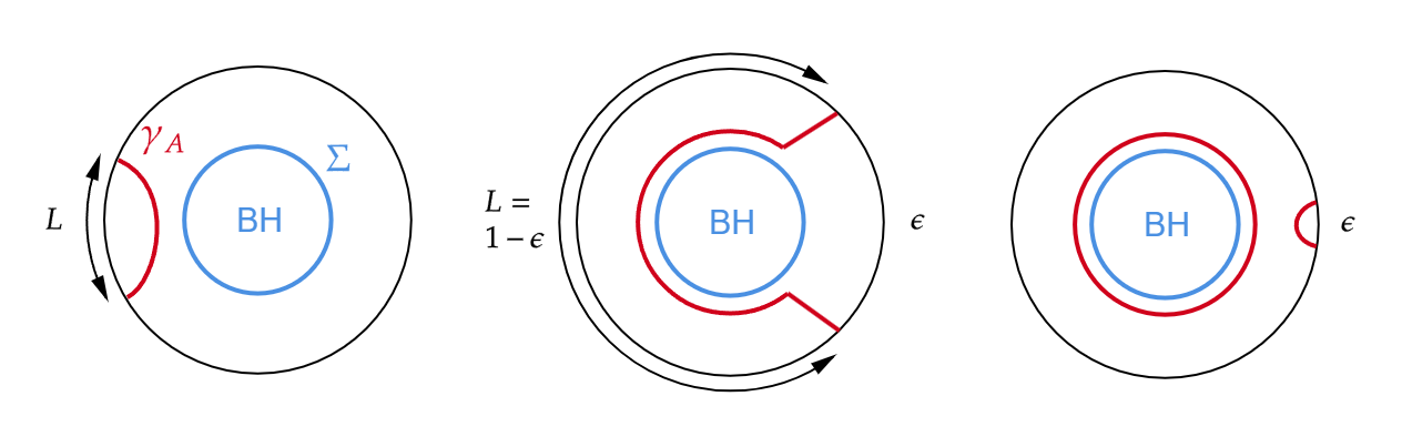
Figure 1: The geodesic length of $\gamma_{A}$ on a time slice of AdS₃ is related to the entanglement entropy of the dual CFT₂ for an entangling region of length $L$. As $L$ increases, the geodesic $\gamma_{A}$ stretches further and eventually wraps around the event horizon of the black hole. In the limit where $L$ becomes sufficiently large, the geodesic $\gamma_{A}$ fully encircles the horizon, and its length coincides with the horizon length. Consequently, the black hole entropy can be extracted from the entanglement entropy in this manner.

However, this setup is challenging to generalize to higher-dimensional black holes. The primary difficulty lies in the lack of a concrete method for computing the entanglement entropy of a CFT_D-1 in higher dimensions. Even if such results were known, it would remain unclear how to construct the corresponding minimal surface $\gamma_{A}$ in the bulk such that it wraps around the higher-dimensional black hole’s event horizon in a manner analogous to the three-dimensional case. To solve this issue, let us revisit the BTZ black hole from a different perspective. Consider the maximally extended Penrose diagram of the BTZ black hole, which features two asymptotic boundaries, each of which hosts a copy of the dual CFT₂ [7]. These two CFTs on asymptotic boundaries are known as the Thermofield double (TFD) sate. Each point in this diagram represents a spatial $S^{1}$ circle, as shown in the left panel of figure (2). From the viewpoint of the boundary CFT₂, we can compute the entanglement entropy $S_{\mathrm{vN}}\left(A:B\right)$ between regions $A$ and $B$ located on the two separate asymptotic boundaries, following recent developments in the study of disconnected-boundary entanglement [8, 9, 10]. Using the RT formula, we obtain the corresponding geodesic $\gamma\left(A:B\right)$, which coincides with the event horizon of the BTZ black hole, as illustrated in the right panel of (2) (Note that the event horizons of the BTZ black hole and the wormhole are identical). In other words, since the holographic dual of the thermofield double (TFD) state and the BTZ black hole share the same Penrose diagram, and both the entanglement entropy and black hole entropy correspond to areas associated with specific points on this diagram, one can use entanglement entropy to probe black hole entropy whenever the corresponding points coincide. Therefore, the entanglement entropy $S_{\mathrm{vN}}\left(A:B\right)$ in a two-boundary configuration of CFT₂ offers a viable approach for recovering the Bekenstein-Hawking entropy of the BTZ black hole.

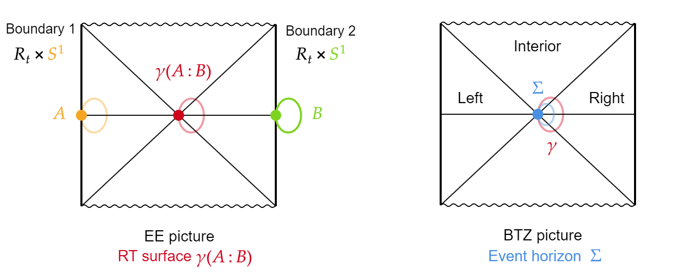
Figure 2: The left panel illustrates the emergence of spacetime from the entanglement entropy of a thermofield double (TFD) state. Two CFTs reside on the two asymptotic boundaries, and at a fixed time slice, each point on the boundary corresponds to an $S^{1}$ circle. The entanglement entropy between two disconnected boundary circles yields the length of the geodesic ${\color[rgb]{1,0,0}\gamma\left(A:B\right)}$. This geodesic ${\color[rgb]{1,0,0}\gamma\left(A:B\right)}$ is precisely the event horizon ${\color[rgb]{0,0,1}\Sigma}$ of the BTZ black hole, as shown in the right panel.

Now, we aim to generalize this method to arbitrary higher-dimensional black holes. The key insight lies in the near-horizon region of near-extremal black holes, as all known extremal black holes exhibit an AdS₂ factor in their near-horizon geometry [11]. Based on this observation, and motivated by the AdS₂/CFT₁ correspondence, it is natural to investigate how the black hole entropy is related to the entanglement entropy in CFT₁. Moreover, it is important to note that the AdS₂ geometry itself possesses a nonzero entropy, as it arises in the near-horizon limit of large $D$ near-extremal black holes [4]. In this paper, we focus on a concrete example: the large $D$ Reissner–Nordström (RN) black hole of Einstein-Maxwell theory. The correspondence between large $D$ black holes and low-dimensional string theory was first observed in ref. [12]. The near-horizon geometry of the extremal RN black hole in the large $D$ limit is AdS₂, which is the solution of two-dimensional heterotic string effective action. This solution allows us to compute the entanglement entropy between two CFT₁ (or more precisely, conformal quantum mechanics, CQM₁) theories defined on the boundaries of AdS₂. Following the same reasoning as in the BTZ black hole case, this entanglement entropy corresponds to a minimal surface $\gamma\left(A:B\right)$, which in turn captures the area of the event horizon of the large $D$ RN black hole, as shown in figure (3). In the entropy, the remaining spherical part of the metric will be absorbed into the $D$-dimensional Newton’s constant $G_{N}^{\left(D\right)}$, effectively reducing it to a two-dimensional quantity, denoted as $G_{N}^{\left(2\right)}$. Thus, it becomes possible to compute the higher-dimensional Bekenstein–Hawking entropy from the entanglement entropy of CQM₁. In the large $D$ limit, the relation between black hole entropy and entanglement entropy becomes particularly transparent: black hole entropy arises entirely from the entanglement entropy between the two CFTs living on either side of the event horizon. In other words, entanglement entropy weaves together the structure of black hole entropy.

Figure 3: The shaded square regions on both sides denote equivalent regions of interest. The left-hand side of the figure shows the Penrose diagram of a $D$-dimensional extremal RN black hole. The strip enclosed by dashed purple lines represents its near-horizon region, which takes the form AdS₂$\times S^{D-2}$. Each point along the bold black line corresponds to the same area of the event horizon. The Bekenstein–Hawking entropy associated with the black hole is entirely determined by the AdS₂ geometry, captured by the blue dot labeled $\mathrm{Area}\left({\color[rgb]{0,0,1}\Sigma}\right)$. In the entropy, the higher-dimensional spherical part $S^{D-2}$ of the spacetime metric is absorbed into the $D$-dimensional Newton’s constant $G_{N}^{\left(D\right)}$, effectively reducing it to a two-dimensional Newton’s constant, denoted $G_{N}^{\left(2\right)}$. The right-hand side of the figure illustrates the emergent AdS₂ spacetime derived from the entanglement entropy of a TFD state. In this setup, the RT prescription yields the area associated with the red dot $\mathrm{Area}\left({\color[rgb]{1,0,0}\gamma\left(A:B\right)}\right)$. Since the two purple strip regions represent the same near-horizon geometry, the areas can be naturally identified: $\mathrm{Area}\left({\color[rgb]{0,0,1}\Sigma}\right)=\mathrm{Area}\left({\color[rgb]{1,0,0}\gamma\left(A:B\right)}\right)$. This observation implies that the $D$-dimensional Bekenstein–Hawking entropy of the extremal black hole can be recovered from the entanglement entropy of CQM₁.

Several related studies are worth mentioning here. In [13], the authors investigate the large $D$ limit of Reissner–Nordström–AdS (RN-AdS) black holes in both extremal and non-extremal cases. They show that the near-horizon geometry of the extremal case becomes AdS₂, and the Bekenstein–Hawking entropy is computed using the Cardy formula. Another relevant work examines the island formula in the context of large $D$ RN-AdS black holes [14]. In [15], the large $D$ limit of Lifshitz black holes is studied. The authors find that the near-horizon and near-extremal regions are effectively captured by two-dimensional gravity theories, including the Callan–Giddings–Harvey–Strominger (CGHS) and Jackiw–Teitelboim (JT) models.

This paper is organized as follows. In Section 2, we review the entanglement entropy of finite regions in the TFD state. This result can be applied to extract the Bekenstein–Hawking entropy of the BTZ black hole and the $D1$-$D5$ black hole in type IIB string theory. In Section 3, we generalize the method to the large $D$ RN black hole. As expected, the Bekenstein–Hawking entropy exactly matches the entanglement entropy of CQM₁. The final section contains our conclusions and discussions.

2 Entanglement entropy of the TFD state

In this section, we briefly review the computation of entanglement entropy between two disconnected CFTs in the thermofield double (TFD) formalism. This approach was originally formulated in [8] and further developed in [9, 10]. For a comprehensive review of the TFD state and its associated Euclidean path integral construction, see [16, 17].

2.1 BTZ black hole

We consider the total Hilbert space as the tensor product of two identical CFT Hilbert spaces:

$$\mathcal{H}_{total}=\mathcal{H}_{1}\otimes\mathcal{H}_{2},$$ (2.4)

where each energy eigenstate satisfies $H\left|n\right\rangle=E_{n}\left|n\right\rangle$. The TFD state, a pure entangled state in this doubled system, is defined by

$$\left|TFD\right\rangle=\frac{1}{\sqrt{Z\left(\beta\right)}}\underset{n}{\sum}e^{-\beta E_{n}/2}\left|E_{n}\right\rangle_{1}\otimes\left|E_{n}\right\rangle_{2},\qquad Z\left(\beta\right)=\underset{n}{\sum}e^{-\beta E_{n}},$$ (2.5)

where $T=1/\beta$ denotes the temperature. The corresponding density matrix is given by

$$\rho_{total}=\left|TFD\right\rangle\left\langle TFD\right|.$$ (2.6)

Remarkably, the entropy of system 1 is precisely the entanglement entropy between the two CFT copies, which can be given by:

$$S_{1}=-tr\rho_{1}\ln\rho_{1},$$ (2.7)

where the reduced density matrix is $\rho_{1}=tr_{2}\rho_{total}=e^{-\beta H_{1}}$. Furthermore, the TFD state can be constructed by “cutting” the thermal partition function into two halves, as illustrated in figure (4). Once the TFD state is prepared, one can specify the entangling regions $A$ and $B$ on each respective boundary and compute the corresponding entanglement entropy.

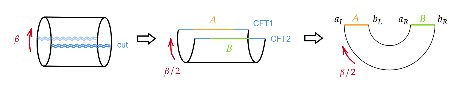
Figure 4: This figure illustrates the preparation of the TFD state. The first step is to consider the thermal partition function at temperature $T=1/\beta$. A quantum field theory (QFT) at finite temperature can be formulated as a Euclidean path integral with imaginary time periodicity, where $t\sim t+i\beta$. For a two-dimensional theory on the line, the corresponding Euclidean geometry is an infinite cylinder with periodicity $\beta$ in the Euclidean time direction. The second step involves cutting this cylinder along a time interval of length $\beta/2$, effectively dividing it into two halves. Two copies of the CFT are then defined on the two resulting blue boundaries, representing the open cuts. Upon specifying entangling regions $A$ and $B$ on each side, the relevant path integral region corresponds to a half-annulus geometry.

The corresponding entanglement entropy in the annular CFT can be computed using the modular Hamiltonian method, and is given by the replica trick:

$$S_{\mathrm{vN}}\left(A:B\right)=\underset{N\rightarrow 1}{\lim}\left[\frac{1}{1-N}\log tr_{A}\rho_{A}^{N}\right]=\underset{N\rightarrow 1}{\lim}\left[\frac{1}{1-N}\log\frac{Z_{N}}{Z_{1}^{N}}\right],$$ (2.8)

where $Z_{1}$ denotes the ordinary annulus partition function with width $W=\log\frac{R_{2}}{R_{1}}$, and $Z_{N}$ represents the partition function on the replicated manifold, which is conformally equivalent to an annulus of width $W_{N}=\frac{W}{N}$, as illustrated in figure (5).

Figure 5: The left-hand side of the figure depicts a standard annulus geometry, whose corresponding partition function is denoted by $Z_{1}$. The width of the annulus is given by $W=\log\frac{R_{2}}{R_{1}}$, where $R_{1}$ and $R2$ are the inner and outer radii, respectively. After applying the replica trick to compute the entanglement entropy, the geometry is modified to a replicated annulus shown on the right-hand side. This replicated geometry has a reduced width $W_{N}=\frac{W}{N}$, and the associated partition function is denoted by $Z_{N}$.

Using this setup, the entanglement entropy becomes

$$S_{\mathrm{vN}}\left(A:B\right)=\frac{c}{6}\log\left(1+2\eta^{-1}+2\sqrt{\eta^{-1}\left(\eta^{-1}+1\right)}\right),$$ (2.9)

where we neglect boundary contributions, which do not affect the universal part of the result. The cross-ratio $\eta$ is defined as

$$\eta=\frac{\cosh\left(\frac{\pi\left(a_{L}-a_{R}\right)}{\beta}\right)\cosh\left(\frac{\pi\left(b_{L}-b_{R}\right)}{\beta}\right)}{\sinh\left(\frac{\pi\left(a_{L}-b_{L}\right)}{\beta}\right)\sinh\left(\frac{\pi\left(a_{R}-b_{R}\right)}{\beta}\right)}.$$ (2.10)

By applying the coordinate transformation described in [10], and specializing to the case $a_{L}=a_{R}=a$ and $b_{L}=b_{R}=b$, the expression simplifies to

$$S_{\mathrm{vN}}\left(A:B\right)=\frac{\pi c}{3\beta}\left|a-b\right|.$$ (2.11)

Using the AdS/CFT dictionary: $c=3R_{AdS}/2G_{N}^{\left(3\right)}$, $\frac{\left|a-b\right|}{\beta}=\frac{r_{+}}{R_{AdS}}$, and the Hawking temperature $\beta=\frac{2\pi R_{AdS}^{2}}{r_{+}}$, we obtain

$$S_{\mathrm{vN}}\left(A:B\right)=\frac{2\pi r_{+}}{4G_{N}^{\left(3\right)}}.$$ (2.12)

This value precisely reproduces the area of the red point (entangling surface) according to the RT formula in figure (6), which coincides with the area of the BTZ black hole event horizon $\Sigma$, since the entanglement entropy and black hole entropy correspond to the same surface in the shared Penrose diagram of the TFD state and BTZ geometry. Therefore, we conclude:

$$S_{\mathrm{vN}}\left(A:B\right)=S_{BH},$$ (2.13)

establishing a direct identification between entanglement entropy in the TFD state and the Bekenstein–Hawking entropy of the BTZ black hole.

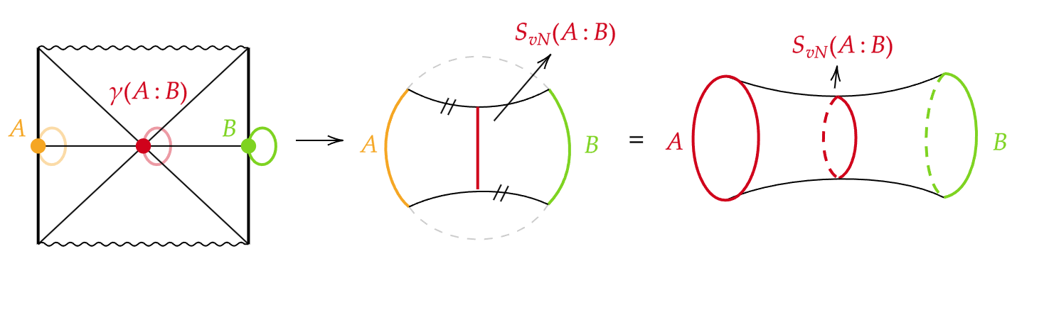
Figure 6: This picture illustrates the spacetime that emerges from the entanglement entropy of the TFD state. The spacetime geometry is reconstructed via Synge’s world function associated with the von Neumann entanglement entropy $S_{\mathrm{vN}}\left(A:B\right)$. In the first panel, each point along the central horizontal line corresponds to an $S^{1}$ circle. Therefore, this horizontal line can be visualized as in the second or third panels. The third panel is obtained as a quotient of the geometry shown in the second panel.

2.2 $D1$-$D5$ black hole of type IIB string theory

A quick example is the $D1$-$D5$ black hole, which arises as a solution of ten-dimensional type IIB string theory with $Q_{1}$ D$1$-branes and $Q_{5}$ D$5$-branes wrapped on a compact internal space $T^{4}\times S^{1}$. Here, the four-torus $T^{4}$ has volume $\left(2\pi\right)^{4}v\alpha^{\prime}$, and the circle $S^{1}$ has radius $R$ [18]. The Kaluza-Klein momentum along $S^{1}$ is quantized and labeled by $N$. The near-horizon limit is obtained by taking the string length squared $\alpha^{\prime}\rightarrow 0$, leading to the following geometry:

$$\frac{dS^{2}}{\alpha^{\prime}}=\left[\frac{U^{2}}{\ell^{2}}\left(-dt^{2}+\left(dx^{5}\right)^{2}\right)+\frac{\ell^{2}}{U^{2}-U_{0}^{2}}dU^{2}\right]+\frac{U_{0}^{2}}{\ell^{2}}\left(\cosh\sigma dt+\sinh\sigma dx^{5}\right)^{2}+\ell^{2}\left(d\Omega_{3}\right)^{2}+\sqrt{\frac{Q_{1}}{vQ_{5}}}dx_{i}^{2},$$ (2.14)

where $\ell^{2}=g_{6}\sqrt{Q_{1}Q_{5}}$, $g_{6}$ is the six-dimensional string coupling, and $x^{5}$ is the coordinate along $S^{1}$. Note $Q_{1}Q_{5}$ also determines the central charge of the dual two-dimensional CFT via the Kac-Moody superconformal algebra. It is evident that the coordinates $\left(x^{5},U,t\right)$ span a locally AdS₃ geometry. Therefore, the full near-horizon geometry (2.14) can be interpreted as

$$\mathrm{BTZ}_{3}\times S^{3}\times T^{4}.$$ (2.15)

The corresponding Bekenstein–Hawking entropy is given by the Cardy formula for the dual CFT:

$$S_{BH}=2\pi\sqrt{\frac{cL_{0}}{6}}=2\pi\sqrt{Q_{1}Q_{5}N}.$$ (2.16)

To probe this result using entanglement entropy, we also compute the entanglement entropy between the two CFTs defined on the asymptotic boundaries. Since the near-horizon region of the $D1$-$D5$ black hole is $\mathrm{BTZ}_{3}$, our previous result for the entanglement entropy of the TFD (2.11) is applicable here. However, given the specific form of the near-horizon metric (2.14), the central charge of the dual CFT must include contributions from both bosonic and fermionic degrees of freedom. This yields [19, 20]:

$$c=6Q_{1}Q_{5}.$$ (2.17)

Furthermore, from the near-horizon metric (2.14), the AdS radius can be identified as

$$R_{AdS}^{2}=\ell^{2}.$$ (2.18)

In the extremal limit, the black hole radius $r_{+}$ is related to the microscopic parameters by [18]:

$$\frac{r_{+}^{2}}{R_{AdS}^{2}}=\frac{N}{Q_{1}Q_{5}}.$$ (2.19)

Substituting this into our general entanglement entropy result (2.11), and using the identification $\frac{\left|a-b\right|}{\beta}=\frac{r_{+}}{R_{AdS}}$, we find

$$S_{\mathrm{vN}}\left(A:B\right)=\frac{\pi c}{3\beta}\left|a-b\right|=2\pi\sqrt{Q_{1}Q_{5}N}.$$ (2.20)

which precisely reproduces the Bekenstein–Hawking entropy given in (2.16). This agreement confirms that our method, based on computing entanglement entropy from the dual CFT, correctly captures the Bekenstein–Hawking entropy of the $D1$-$D5$ black hole, whose near-horizon geometry is BTZ₃.

Moreover, it is worth noting that the near horizon limit of near extremal BTZ is AdS₂$\times S^{1}$. This implies that the corresponding TFD state in AdS₂/CFT₁ can also be used to compute the entanglement entropy. In this case, one starts with a rotating BTZ black hole, which modifies the CFT defined on the asymptotic boundary. The TFD state must then be replaced by [7]:

$$\left|TFD\right\rangle=\frac{1}{\sqrt{Z_{0}}}\underset{n_{L},n_{R}}{\sum}e^{-\frac{\beta_{L}L_{0}}{2}-\frac{\beta_{R}\bar{L}_{0}}{2}}\left|n_{L},n_{R}\right\rangle_{1}\otimes\left|n_{L},n_{R}\right\rangle_{2},$$ (2.21)

where $Z_{0}$ is the partition function of the CFT₂. Consequently, the corresponding entanglement entropy differs from the non-rotating case. This entropy has been computed in [4] by taking the near-extremal limit—where $\beta_{L}$ remains finite and $\beta_{R}\rightarrow\infty$ —and the near-horizon limit $r\rightarrow r_{+}$. In this setup, states labeled by $L_{0}=N$ are denoted as $\left|k\right\rangle$, where $k=1,2,\ldots,d\left(N\right)$. The degeneracy $d\left(N\right)$ is large and grows as:

$$d\left(N\right)\sim e^{2\pi\sqrt{Q_{1}Q_{5}N}}.$$ (2.22)

The TFD state in the near-horizon, near-extremal limit can then be rewritten as

$$\left|TFD\right\rangle=\frac{1}{\sqrt{d\left(N\right)}}\underset{n}{\sum}\underset{k=1}{\overset{d\left(N\right)}{\sum}}e^{-\frac{\beta E_{n}}{2}}\left|k_{L},n_{R}\right\rangle_{\mathrm{CQM}1}\otimes\left|k_{L},n_{R}\right\rangle_{\mathrm{CQM}2},$$ (2.23)

where $E_{n}=\left\langle n\left|\bar{L}_{0}\right|n\right\rangle$. In the zero temperature limit $\beta=\infty$, there is only the single ground state $\left|0\right\rangle$ in the the right-moving sector, and the state reduces to $\left|k\right\rangle_{\mathrm{CQM}1}=\left|k_{L},0\right\rangle$. The reduced density matrix of CQM1, obtained by tracing out CQM2 , is

$$\rho_{1}=\frac{1}{\sqrt{d\left(N\right)}}\underset{k=1}{\overset{d\left(N\right)}{\sum}}\left|k\right\rangle\left\langle k\right|_{\mathrm{CQM}1}.$$ (2.24)

The entanglement entropy then becomes

$$S_{1}=-tr\rho_{1}\ln\rho_{1}=\log d\left(N\right)=2\pi\sqrt{Q_{1}Q_{5}N},$$ (2.25)

which exactly matches our previous result (2.20). This equivalence demonstrates that our approach not only captures the Bekenstein–Hawking entropy but also provides a microscopic counting of BPS states of the black hole.

3 Large $D$ black hole entropy and CQM₁ entanglement entropy

In this section, we demonstrate that the entanglement entropy of a one-dimensional CQM₁ precisely matches the Bekenstein–Hawking entropy of a RN black hole in the large $D$ limit. Specifically, we begin by analyzing the RN black hole in the large $D$ regime, where the near-horizon geometry simplifies and becomes effectively described by a two-dimensional charged black hole—a solution arising from the heterotic string effective action. In the extremal limit, this near-horizon geometry further reduces to AdS₂. Simultaneously, we examine the Bekenstein–Hawking entropy of the RN black hole under the same limiting procedure: large $D$ and extremality. In this limit, the entropy becomes a purely two-dimensional quantity, as the area of the event horizon shrinks to a point (represented by the blue dot in the left panel of figure (7)). On the other hand, we compute the entanglement entropy for two disconnected CQM₁ systems using both field-theoretic and holographic techniques. The results obtained from these independent methods are in complete agreement and yield a minimal surface located at the midpoint of the Penrose diagram (represented by the red dot in the right panel of figure (7)). As expected, this entanglement entropy exactly reproduces the Bekenstein–Hawking entropy of the extremal RN black hole in the large $D$ limit, thereby establishing a precise correspondence between the two.

Figure 7: This figure highlights the shaded regions of interest from figure (3). The purple strip regions on both sides share the same Penrose diagram and describe identical near-horizon geometries. In this section, we demonstrate that the Bekenstein–Hawking entropy of the RN black hole in the large $D$ limit, shown on the left-hand side, precisely matches the entanglement entropy of the CQM₁ on the right-hand side.

3.1 Bekenstein-Hawking entropy of RN black hole at large $D$

In this subsection, we initiate the computation of the large $D$ limit of the RN black hole and its corresponding Bekenstein–Hawking entropy. Given the one-to-one correspondence between black hole solutions and gravitational actions, the large $D$ behavior can be analyzed from two complementary perspectives: the metric description and the action-based formulation. Accordingly, our strategy proceeds along the following route:

3.1.1 RN black hole at large $D$

Metric description:

Let us begin with the first step $①$, where we aim to demonstrate that the large $D$ limit of the RN black hole reduces to the two-dimensional charged black hole solution in string theory. We first recall the $D$-dimensional RN black hole solution in Einstein–Maxwell theory [21]:

$$ds^{2}=-f\left(r\right)dt^{2}+\frac{dr^{2}}{f\left(r\right)}+r^{2}d\Omega_{n+1}^{2}$$ (3.26)

where $D=n+3$, and

$$f\left(r\right)=1-\frac{2m}{r^{n}}+\frac{q^{2}}{r^{2n}},\qquad A_{t}=\sqrt{\frac{n+1}{2n}}\left(C-\frac{q}{r^{n}}\right)dt,$$ (3.27)

with $C$ an arbitrary constant. The parameters $m$ and $q$ are related to the ADM mass $M$ and the physical electric charge $Q$ via:

$$m=\frac{8\pi}{\Omega_{n+1}\left(n+1\right)}M,\qquad q^{2}=\frac{2}{\left(n+1\right)n}Q^{2},\qquad\Omega_{n+1}=\frac{2\pi^{\left(n+2\right)/2}}{\Gamma\left(\frac{n+2}{2}\right)}.$$ (3.28)

The inner and outer horizons $r_{\pm}$ are determined by the roots of:

$$1-\frac{r_{0}^{n}}{r^{n}}+\frac{q^{2}}{r^{2n}}=0,$$ (3.29)

where we define $r_{0}^{n}\equiv 2m$, so that $\mathrm{dim}\left[r_{0}\right]=\mathrm{Length}$. Accordingly, $\mathrm{dim}\left[m\right]=\mathrm{dim}\left[q\right]=\mathrm{Length}^{n}$. The horizon locations are given by:

$$r_{\pm}^{n}=\frac{1}{2}r_{0}^{n}\pm\sqrt{\frac{1}{4}r_{0}^{2n}-q^{2}}.$$ (3.30)

In the extremal case, the condition $q^{2}=\frac{1}{4}r_{0}^{2n}$ yields a degenerate horizon at:

$$r_{h}^{n}\equiv r_{\pm}^{n}=\frac{1}{2}r_{0}^{n}=m.$$ (3.31)

To study the near-horizon geometry, we introduce the dimensionless coordinate:

$$\mathrm{R}=\left(\frac{r}{r_{0}}\right)^{n},$$ (3.32)

Before proceeding, it is worth emphasizing that the notion of the event horizon differs significantly between finite and large $D$. To see this, we express $f\left(r\right)$ in terms of $\mathrm{R}$:

$$f\left(\mathrm{R}\right)=1-\frac{1}{\mathrm{R}}+\frac{q^{2}}{\left(2m\right)^{2}}\frac{1}{\mathrm{R}^{2}}.$$ (3.33)

It follows that:

$$\mathrm{R}_{\pm}=\left(\frac{r_{\pm}}{r_{0}}\right)^{n}\Rightarrow r_{\pm}=r_{0}\mathrm{R}_{\pm}^{\frac{1}{n}}\rightarrow r_{\pm}=r_{0},$$ (3.34)

in the large $D$ limit. This result clearly contrasts with the finite $D$ case (3.31). Let us now rewrite the metric in terms of the coordinate $\mathrm{R}$:

$$ds^{2} = -\left(1-\frac{1}{\mathrm{R}}+\frac{q^{2}}{\left(2m\right)^{2}}\frac{1}{\mathrm{R}^{2}}\right)dt^{2}+\left(\frac{r_{0}}{n}\right)^{2}\frac{\mathrm{R}^{\frac{2\left(1-n\right)}{n}}d\mathrm{R}^{2}}{\left(1-\frac{1}{\mathrm{R}}+\frac{q^{2}}{\left(2m\right)^{2}}\frac{1}{\mathrm{R}^{2}}\right)}+r_{0}^{2}\mathrm{R}^{\frac{2}{n}}d\Omega_{n+1}^{2},$$

$$A_{t} = \sqrt{\frac{n+1}{2n}}\left(C-\frac{q}{r_{0}^{n}\mathrm{R}}\right)dt.$$ (3.35)

Note that we have not assumed $\mathrm{R}=\mathrm{R}_{\pm}$, so this result holds for both extremal and non-extremal cases. In the large $D$ limit (i.e., $\ln\mathrm{R}\ll n$), the metric simplifies to:

$$ds^{2} = -\left(1-\frac{1}{\mathrm{R}}+\frac{q^{2}}{\left(2m\right)^{2}}\frac{1}{\mathrm{R}^{2}}\right)dt^{2}+\left(\frac{r_{0}}{n}\right)^{2}\frac{d\mathrm{R}^{2}}{\mathrm{R}^{2}\left(1-\frac{1}{\mathrm{R}}+\frac{q^{2}}{\left(2m\right)^{2}}\frac{1}{\mathrm{R}^{2}}\right)}+r_{0}^{2}d\Omega_{n+1}^{2},$$

$$A_{t} = \sqrt{\frac{1}{2}}\left(C-\frac{q}{\mathrm{R}}\frac{1}{r_{0}^{n}}\right)dt.$$ (3.36)

To restore the physical radial dimension, we define:

$$\mathrm{R}=\frac{\bar{\mathrm{R}}}{2m},\qquad 2\lambda=\frac{n}{r_{0}}.$$ (3.37)

Since $\bar{\mathrm{R}}=2m\frac{r^{n}}{r_{0}^{n}}=r^{n}$, this transformation connects $\bar{\mathrm{R}}$ with the $n$-th power of the physical radius $r$. This form precisely matches the two-dimensional charged black hole solution of heterotic string theory [22, 23]:

$$ds^{2} = -\left(1-\frac{2m}{\bar{\mathrm{R}}}+\frac{q^{2}}{\bar{\mathrm{R}}^{2}}\right)dt^{2}+\frac{d\bar{\mathrm{R}}^{2}}{\mathrm{\left(2\lambda\right)}^{2}\bar{\mathrm{R}}^{2}\left(1-\frac{2m}{\bar{\mathrm{R}}}+\frac{q^{2}}{\bar{\mathrm{R}}^{2}}\right)}+r_{0}^{2}d\Omega_{n+1}^{2},$$

$$A_{t} = \sqrt{\frac{1}{2}}\left(\frac{q}{\bar{\mathrm{R}}_{+}}-\frac{q}{\bar{\mathrm{R}}}\right)dt.$$ (3.38)

with field strength $F^{2}=-\frac{4\lambda^{2}q^{2}}{\bar{\mathrm{R}}^{2}}$. The gauge potential is fixed by requiring $A_{t}\left(\bar{\mathrm{R}}_{+}\right)=0$. The dilaton field in this background is given by $\phi\left(\bar{\mathrm{R}}\right)=-\frac{1}{2}\ln\frac{\bar{\mathrm{R}}}{2m}$, which can be derived from the corresponding low-energy effective action.

Action description:

Now, we consider step $②$, which involves the action description corresponding to the black hole solution obtained in step $①$. We begin with the $D$-dimensional Einstein–Maxwell theory, whose action is given by:

$$I_{\mathrm{EM}}=\frac{1}{16\pi G_{N}^{\left(D\right)}}\int d^{D}x\sqrt{-g}\left(R-F_{\mu\nu}F^{\mu\nu}\right)$$ (3.39)

To introduce a dilaton field $\phi(x^{\mu})$, we perform a dimensional reduction on a $\left(n+1\right)$-dimensional sphere, with the following ansatz for the metric:

$$ds^{2}=\underset{2\;\mathrm{dimensions}}{\underbrace{\mathbb{G}_{\mu\nu}\left(x^{\mu}\right)dx^{\mu}dx^{\nu}}}+\underset{n+1\;\mathrm{dimensional\;sphere}}{\underbrace{r_{0}^{2}e^{-4\phi\left(x^{\mu}\right)/\left(n+1\right)}d\Omega_{n+1}^{2}}},$$ (3.40)

where $\mathbb{G}_{\mu\nu}$ is the two-dimensional metric, and $d\Omega_{n+1}^{2}$ is the line element of a unit $\left(n+1\right)$-sphere. Under this reduction, the Einstein–Maxwell action becomes:

$$I_{\mathrm{EM}}=\frac{\Omega_{n+1}r_{0}^{n+1}}{16\pi G_{N}^{\left(D\right)}}\int d^{2}x\sqrt{-\mathbb{G}}e^{-2\phi}\left(\mathbb{R}+\frac{4n}{n+1}\left(\nabla\phi\right)^{2}+\frac{n\left(n+1\right)}{r_{0}^{2}}e^{-4\phi/\left(n+1\right)}-F_{\mu\nu}F^{\mu\nu}\right),$$ (3.41)

where $\mathbb{R}$ is the Ricci scalar associated with the 2$D$ metric, and the volume of the unit $\left(n+1\right)$-sphere is given by $\Omega_{n+1}=2\pi^{\frac{n+2}{2}}/\Gamma\left(\frac{n+2}{2}\right)$. Taking the large $n$ limit ($n\rightarrow\infty$), the action reduces to the two-dimensional string effective action:

$$I_{\mathrm{string}}=\frac{1}{16\pi G_{N}^{\left(2\right)}}\int d^{2}x\sqrt{-\mathbb{G}}e^{-2\phi}\left(\mathbb{R}+4\left(\nabla\phi\right)^{2}+4\lambda^{2}-F^{2}\right),$$ (3.42)

where $\lambda=\frac{n}{2r_{0}}$, and the effective two-dimensional Newton’s constant is given by

$$G_{N}^{\left(2\right)}=\underset{n\rightarrow\infty}{\lim}\frac{G_{N}^{\left(D\right)}}{\Omega_{n+1}r_{0}^{n+1}}.$$ (3.43)

This is precisely the two-dimensional heterotic string effective action. To determine the dilaton profile, we compare the metrics (3.26) and (3.40), which leads to:

$$\phi\left(\mathrm{R}\right)=-\frac{n+1}{2n}\ln\mathrm{R}\overset{n\rightarrow\infty}{\longrightarrow}-\frac{1}{2}\ln\mathrm{R}.$$ (3.44)

Applying the same coordinate transformation on $\mathrm{R}$ as used in (3.37), we obtain the dilaton solution in terms of the rescaled coordinate $\bar{\mathrm{R}}$:

$$\phi\left(\bar{\mathrm{R}}\right)=-\frac{1}{2}\ln\frac{\bar{\mathrm{R}}}{2m}.$$ (3.45)

3.1.2 Extremal limit of RN black hole at large $D$

Metric description:

In this subsection, we proceed to discuss steps $③$ and $④$, which involve taking the extremal limit of the large $D$ black hole and analyzing its associated action. Recall that the inner and outer horizons of a large $D$ black hole are determined by the condition:

$$1-\frac{2m}{\bar{\mathrm{R}}}+\frac{q^{2}}{\bar{\mathrm{R}}^{2}}=0,$$ (3.46)

Solving this equation yields the inner and outer horizons $\bar{\mathrm{R}}_{\pm}$:

$$\bar{\mathrm{R}}_{\pm}=m\pm\sqrt{m^{2}-q^{2}},$$ (3.47)

or, equivalently,

$$\bar{\mathrm{R}}_{+}+\bar{\mathrm{R}}_{-}=2m,\qquad\bar{\mathrm{R}}_{+}\bar{\mathrm{R}}_{-}=q^{2}.$$ (3.48)

Using this notation, the black hole metric can be rewritten as:

$$ds^{2}=-\frac{1}{\bar{\mathrm{R}}^{2}}\left(\bar{\mathrm{R}}-\bar{\mathrm{R}}_{+}\right)\left(\bar{\mathrm{R}}-\bar{\mathrm{R}}_{-}\right)dt^{2}+\left(\frac{r_{0}}{n}\right)^{2}\frac{d\bar{\mathrm{R}}^{2}}{\left(\bar{\mathrm{R}}-\bar{\mathrm{R}}_{+}\right)\left(\bar{\mathrm{R}}-\bar{\mathrm{R}}_{-}\right)}+r_{0}^{2}d\Omega_{D-2}^{2},$$ (3.49)

with gauge field and dilaton:

$$A_{t}=\sqrt{\frac{1}{2}}\frac{q}{\bar{\mathrm{R}}_{+}}\left(1-\frac{\bar{\mathrm{R}}_{+}}{\bar{\mathrm{R}}}\right)dt,\qquad\phi\left(\bar{\mathrm{R}}\right)=-\frac{1}{2}\ln\frac{\bar{\mathrm{R}}}{2m}.$$ (3.50)

To study the near-extremal and near-horizon limit, we follow the coordinate transformations introduced in [13]:

$$\bar{\mathrm{R}}\rightarrow\bar{\mathrm{R}}_{+}+\epsilon\tilde{\mathrm{R}},\qquad\bar{\mathrm{R}}_{+}-\bar{\mathrm{R}}_{-}=\epsilon,\qquad t\rightarrow\frac{\bar{\mathrm{R}}_{+}}{\epsilon}\frac{r_{0}}{n}\tau.$$ (3.51)

Applying this limit, the metric becomes

$$ds^{2} = \left(\frac{r_{0}}{n}\right)^{2}\left[-\left(\tilde{\mathrm{R}}\right)\left(\tilde{\mathrm{R}}+1\right)d\tau^{2}+\frac{d\tilde{\mathrm{R}}^{2}}{\left(\tilde{\mathrm{R}}\right)\left(1+\tilde{\mathrm{R}}\right)}\right]+r_{0}^{2}d\Omega_{D-2}^{2},$$

$$A_{\tau} = \sqrt{\frac{1}{2}}\frac{q}{\bar{\mathrm{R}}_{+}}\tilde{\mathrm{R}}\frac{r_{0}}{n}d\tau,$$

$$\phi\left(\bar{\mathrm{R}}\right) = -\frac{1}{2}\ln\frac{\bar{\mathrm{R}}_{+}}{2m}.$$ (3.52)

We can also rewrite the metric as:

$$ds^{2}=\left(\frac{r_{0}}{n}\right)^{2}\left[-\left(\left(\tilde{\mathrm{R}}+\frac{1}{2}\right)^{2}-\frac{1}{4}\right)d\tau^{2}+\frac{d\tilde{\mathrm{R}}^{2}}{\left(\left(\tilde{\mathrm{R}}+\frac{1}{2}\right)^{2}-\frac{1}{4}\right)}\right]+r_{0}^{2}d\Omega_{D-2}^{2}.$$ (3.53)

Introducing a new coordinate:

$$\rho=\tilde{\mathrm{R}}+\frac{1}{2},$$ (3.54)

and in the extremal limit, where $q=\bar{\mathrm{R}}_{+}=m$, the geometry becomes:

$$ds^{2} = \left(\frac{r_{0}}{n}\right)^{2}\left[-\left(\rho^{2}-\frac{1}{4}\right)d\tau^{2}+\frac{d\rho^{2}}{\left(\rho^{2}-\frac{1}{4}\right)}\right]+r_{0}^{2}d\Omega_{D-2}^{2},$$

$$A_{\tau} = \sqrt{\frac{1}{2}}\frac{r_{0}}{n}\left(\rho-\frac{1}{2}\right)d\tau,$$

$$\phi\left(\rho\right) = -\frac{1}{2}\ln\frac{1}{2}.$$ (3.55)

The field strength squared becomes: $F^{2}=-\frac{4\lambda^{2}q^{2}}{\bar{\mathrm{R}}^{2}}=-4\lambda^{2}$. We observe that the $\left(\tau,\rho\right)$ sector of the geometry is precisely AdS₂, completing the near-horizon, extremal limit of the large $D$ charged black hole.

Action description:

Finally, let us see how the two-dimensional heterotic string effective action reduces to two-dimensional gravity in the extremal limit. Recall the two-dimensional heterotic string effective action:

$$I_{\mathrm{string}}=\frac{1}{16\pi G_{N}^{\left(2\right)}}\int d^{2}x\sqrt{-\mathbb{G}}e^{-2\phi}\left(\mathbb{R}+4\left(\nabla\phi\right)^{2}+4\lambda^{2}-F^{2}\right).$$ (3.56)

In the extremal limit, we use the constant dilaton solution $\phi\left(\bar{\mathrm{R}}\right)=-\frac{1}{2}\ln\frac{1}{2}$ given earlier to integrate out the dilaton. The action then becomes

$$I_{\mathrm{string}}=\frac{1}{16\pi G_{N}^{\left(2\right)}}\int d^{2}xe^{-2\phi}\sqrt{-\mathbb{G}}\left(\mathbb{R}+4\lambda^{2}-F^{2}\right),$$ (3.57)

which corresponds to Jackiw–Teitelboim (JT) gravity without the topological term. The solution to this action is

$$\mathbb{R}=-8\lambda^{2},\qquad F^{2}=-\frac{4\lambda^{2}q^{2}}{\bar{\mathrm{R}}^{2}}=-4\lambda^{2},$$ (3.58)

which agrees with the AdS₂ solution obtained previously in the metric formulation (3.55).

3.1.3 Bekenstein-Hawking entropy

Now let us examine the Bekenstein–Hawking entropy of an extremal RN black hole in the large $D$ limit. We begin by recalling the $D$-dimensional RN black hole metric (3.26):

$$ds^{2}=-f\left(r\right)dt^{2}+\frac{dr^{2}}{f\left(r\right)}+r^{2}d\Omega_{n+1}^{2},$$ (3.59)

where $D=n+3$, and

$$f\left(r\right)=1-\frac{2m}{r^{n}}+\frac{q^{2}}{r^{2n}},\qquad A_{t}=\sqrt{\frac{n+1}{2n}}\left(\frac{q}{r_{+}^{n}}-\frac{q}{r^{n}}\right)dt,$$ (3.60)

where the gauge potential is fixed by requiring $A_{t}\left(r_{+}\right)=0$. The Bekenstein–Hawking entropy in $D$ dimensions is given by

$$S_{\mathrm{BH}}=\frac{\mathrm{Area}_{D}}{4G_{N}^{\left(D\right)}}=\frac{r_{+}^{D-2}\Omega_{D-2}}{4G_{N}^{\left(D\right)}}.$$ (3.61)

where we used the fact that the horizon area is $\mathrm{Area}_{D}=r_{+}^{D-2}\Omega_{D-2}$. Using the relation between the two-dimensional and $D$-dimensional Newton constants at large $D$, as derived in equation (3.43):

$$G_{N}^{\left(2\right)}=\underset{n\rightarrow\infty}{\lim}\frac{G_{N}^{\left(D\right)}}{\Omega_{n+1}r_{0}^{n+1}},$$ (3.62)

and applying the extremality condition $r_{+}^{n+1}=r_{0}^{n+1}$ from equation (3.34), the Bekenstein-Hawking entropy becomes

$$S_{\mathrm{BH}}=\frac{1}{4G_{N}^{\left(2\right)}}.$$ (3.63)

3.2 CQM₁ entanglement entropy

Recall the entanglement entropy of the TFD state in the CFT₂ obtained previously (2.11):

$$S_{\mathrm{vN}}\left(A:B\right)=\frac{2\pi r_{+}}{4G_{N}^{\left(3\right)}}.$$ (3.64)

It is straightforward to obtain the entanglement entropy of the CQM₁ using the well-known dimensional reduction formula for Newton’s constant:

$$\frac{1}{G_{N}^{\left(2\right)}}=\frac{2\pi r_{+}}{G_{N}^{\left(3\right)}}.$$ (3.65)

Therefore, we find

$$S_{\mathrm{vN}}\left(A:B\right)=\frac{1}{4G_{N}^{\left(2\right)}},$$ (3.66)

which exactly reproduces the Bekenstein–Hawking entropy (3.63) of the large $D$ extremal RN black hole.

This result can also be verified holographically, following the method of ref.  [4]. Let us recall the two-dimensional gravity action in Euclidean signature, which arises from the large $D$ limit of Einstein–Maxwell theory:

$$I_{\mathrm{string}}=-\frac{1}{16\pi G_{2}}\int d^{2}x\sqrt{\mathbb{G}}e^{-2\phi}\left(\mathbb{R}+4\lambda^{2}-F^{2}\right),$$ (3.67)

where $\lambda=\frac{n}{2r_{0}}$. Using the classical solutions $\phi=\mathrm{const}.$, $A_{t}=\sqrt{\frac{1}{2}}\frac{n}{r_{0}}\left(\rho-\frac{1}{2}\right)d\tau,$ and the field strength $F^{2}=-\frac{4\lambda^{2}q^{2}}{\bar{\mathrm{R}}^{2}}=-4\lambda^{2}$, one introduces the replica geometry via the curvature singularity $\mathbb{R}=4\pi\left(1-N\right)\delta^{2}\left(x\right)$. This leads to the action: $I_{\mathrm{string}}=\frac{N-1}{4G_{N}^{\left(2\right)}}$. The entanglement entropy is then computed by

$$S_{\mathrm{EE}}=-\frac{\partial}{\partial N}\log\left.\left(e^{-I_{\mathrm{string}}+NI_{\mathrm{string}}^{\left(0\right)}}\right)\right|_{n=1}=\frac{1}{4G_{N}^{\left(2\right)}},$$ (3.68)

where $I_{\mathrm{string}}^{\left(0\right)}$ denotes the action of the single-sheeted geometry without any branch cut. This holographic result confirms the field theory calculation (3.66).

Moreover, the same result is supported by recent developments in the nearly-AdS₂/SYK correspondence [24].

4 Conclusion and discussion

In this paper, we developed a method to probe the Bekenstein–Hawking entropy of black holes via entanglement entropy. This approach is based on two key observations. On the gravitational side, the near-horizon geometry of extremal black holes is AdS₂, and the Bekenstein–Hawking entropy is entirely determined by this two-dimensional geometry. The higher-dimensional spherical part of the black hole metric is absorbed into the $D$-dimensional Newton’s constant $G_{N}^{\left(D\right)}$, which can be effectively reduced to a two-dimensional Newton’s constant $G_{N}^{\left(2\right)}$. On the field theory side, the entanglement entropy of two disconnected CQM₁ systems corresponds to the same AdS₂ geometry. According to the RT prescription, this entanglement entropy computes the area of a minimal surface. Since the near-horizon region of the black hole and the emergent spacetime derived from entanglement share the same Penrose diagram—with both the black hole event horizon and the RT surface corresponding to specific points on this diagram—the Bekenstein–Hawking entropy can be extracted from entanglement entropy when these points coincide.

We explicitly verified this correspondence in three examples: the BTZ black hole, the $D1$-$D5$ black hole in type IIB string theory, and the large $D$ RN black hole.

Our results suggest the following:

• Entanglement across the event horizon is the origin of the Bekenstein–Hawking entropy. In other words, information in $D$ spacetime dimensions can be encoded within a one-dimensional quantum system.

• Entanglement entropy provides a route to microscopically count the BPS states of black holes. This is because the RT formula bridges quantum features (states) and classical geometry (minimal surfaces), and the minimal surface in the near-horizon region corresponds to the black hole event horizon.

For future work, a promising direction is:

• Extension to the covariant case. It would be important to generalize this method to time-dependent or non-static geometries, potentially involving the covariant holographic entanglement entropy framework.

Acknowledgements This work was supported by NSFC Grant No. 12105031 and No. 12347101.

References

- [1] L. Susskind and J. Uglum, “Black hole entropy in canonical quantum gravity and superstring theory,” Phys. Rev. D 50, 2700-2711 (1994) doi:10.1103/PhysRevD.50.2700 [arXiv:hep-th/9401070 [hep-th]].
- [2] T. M. Fiola, J. Preskill, A. Strominger and S. P. Trivedi, “Black hole thermodynamics and information loss in two-dimensions,” Phys. Rev. D 50, 3987-4014 (1994) doi:10.1103/PhysRevD.50.3987 [arXiv:hep-th/9403137 [hep-th]].
- [3] T. Jacobson, “Black hole entropy and induced gravity,” [arXiv:gr-qc/9404039 [gr-qc]].
- [4] T. Azeyanagi, T. Nishioka and T. Takayanagi, “Near Extremal Black Hole Entropy as Entanglement Entropy via AdS(2)/CFT(1),” Phys. Rev. D 77, 064005 (2008) doi:10.1103/PhysRevD.77.064005 [arXiv:0710.2956 [hep-th]].
- [5] R. Emparan, “Black hole entropy as entanglement entropy: A Holographic derivation,” JHEP 06, 012 (2006) doi:10.1088/1126-6708/2006/06/012 [arXiv:hep-th/0603081 [hep-th]].
- [6] R. Emparan, G. T. Horowitz and R. C. Myers, “Exact description of black holes on branes,” JHEP 01, 007 (2000) doi:10.1088/1126-6708/2000/01/007 [arXiv:hep-th/9911043 [hep-th]].
- [7] J. M. Maldacena, “Eternal black holes in anti-de Sitter,” JHEP 04, 021 (2003) doi:10.1088/1126-6708/2003/04/021 [arXiv:hep-th/0106112 [hep-th]].
- [8] J. Cardy and E. Tonni, “Entanglement hamiltonians in two-dimensional conformal field theory,” J. Stat. Mech. 1612, no.12, 123103 (2016) doi:10.1088/1742-5468/2016/12/123103 [arXiv:1608.01283 [cond-mat.stat-mech]].
- [9] X. Jiang, P. Wang, H. Wu and H. Yang, “Alternative to purification in conformal field theory,” Phys. Rev. D 111, no.2, L021902 (2025) doi:10.1103/PhysRevD.111.L021902 [arXiv:2406.09033 [hep-th]].
- [10] X. Jiang, P. Wang, H. Wu and H. Yang, “Realization of ”ER=EPR”,” [arXiv:2411.18485 [hep-th]].
- [11] A. Sen, “Quantum Entropy Function from AdS(2)/CFT(1) Correspondence,” Int. J. Mod. Phys. A 24, 4225-4244 (2009) doi:10.1142/S0217751X09045893 [arXiv:0809.3304 [hep-th]].
- [12] R. Emparan, D. Grumiller and K. Tanabe, “Large-D gravity and low-D strings,” Phys. Rev. Lett. 110, no.25, 251102 (2013) doi:10.1103/PhysRevLett.110.251102 [arXiv:1303.1995 [hep-th]].
- [13] E. D. Guo, M. Li and J. R. Sun, “CFT dual of charged AdS black hole in the large dimension limit,” Int. J. Mod. Phys. D 25, no.07, 1650085 (2016) doi:10.1142/S0218271816500851 [arXiv:1512.08349 [gr-qc]].
- [14] C. W. Tong, D. H. Du and J. R. Sun, “Island of Reissner-Nordström anti–de Sitter black holes in the large D limit,” Phys. Rev. D 109, no.10, 104053 (2024) doi:10.1103/PhysRevD.109.104053 [arXiv:2306.06682 [hep-th]].
- [15] W. Sybesma, “A zoo of deformed Jackiw-Teitelboim models near large dimensional black holes,” JHEP 01, 141 (2023) doi:10.1007/JHEP01(2023)141 [arXiv:2211.07927 [hep-th]].
- [16] T. Hartman, “Lectures on Quantum Gravity and Black Holes.”
- [17] N. Callebaut, “Entanglement in Conformal Field Theory and Holography,” Lect. Notes Phys. 1022, 239-271 (2023) doi:10.1007/978-3-031-42096-2_10 [arXiv:2303.16827 [hep-th]].
- [18] J. M. Maldacena and A. Strominger, “AdS(3) black holes and a stringy exclusion principle,” JHEP 12, 005 (1998) doi:10.1088/1126-6708/1998/12/005 [arXiv:hep-th/9804085 [hep-th]].
- [19] A. Strominger and C. Vafa, “Microscopic origin of the Bekenstein-Hawking entropy,” Phys. Lett. B 379, 99-104 (1996) doi:10.1016/0370-2693(96)00345-0 [arXiv:hep-th/9601029 [hep-th]].
- [20] C. G. Callan and J. M. Maldacena, “D-brane approach to black hole quantum mechanics,” Nucl. Phys. B 472, 591-610 (1996) doi:10.1016/0550-3213(96)00225-8 [arXiv:hep-th/9602043 [hep-th]].
- [21] R. C. Myers and M. J. Perry, “Black Holes in Higher Dimensional Space-Times,” Annals Phys. 172, 304 (1986) doi:10.1016/0003-4916(86)90186-7
- [22] M. D. McGuigan, C. R. Nappi and S. A. Yost, “Charged black holes in two-dimensional string theory,” Nucl. Phys. B 375, 421-450 (1992) doi:10.1016/0550-3213(92)90039-E [arXiv:hep-th/9111038 [hep-th]].
- [23] A. Giveon and D. Kutasov, “The Charged black hole/string transition,” JHEP 01, 120 (2006) doi:10.1088/1126-6708/2006/01/120 [arXiv:hep-th/0510211 [hep-th]].
- [24] Y. Chen and P. Zhang, “Entanglement Entropy of Two Coupled SYK Models and Eternal Traversable Wormhole,” JHEP 07, 033 (2019) doi:10.1007/JHEP07(2019)033 [arXiv:1903.10532 [hep-th]].