Tagging fully hadronic exotic decays of the vectorlike $\mathbf{B}$ quark using a graph neural network

Abstract

Following up on our earlier study in [J. Bardhan et al., Machine learning-enhanced search for a vectorlike singlet B quark decaying to a singlet scalar or pseudoscalar, Phys. Rev. D 107 (2023) 115001; arXiv:2212.02442 [hep-ph]], we investigate the LHC prospects of pair-produced vectorlike $B$ quarks decaying exotically to a new gauge-singlet (pseudo)scalar field $\Phi$ and a $b$ quark. After the electroweak symmetry breaking, the $\Phi$ decays predominantly to $gg/bb$ final states, leading to a fully hadronic $2b+4j$ or $6b$ signature. Because of the large Standard Model background and the lack of leptonic handles, it is a difficult channel to probe. To overcome the challenge, we employ a hybrid deep learning model containing a graph neural network followed by a deep neural network. We estimate that such a state-of-the-art deep learning analysis pipeline can lead to a performance comparable to that in the semi-leptonic mode, taking the discovery (exclusion) reach up to about $M_{B}=1.8\>(2.4)$ TeV at HL-LHC when $B$ decays fully exotically, i.e., BR$(B\to b\Phi)=100\%$.

I Introduction

New fermions are usually considered vectorlike in scenarios beyond the Standard Model (SM) to avoid introducing gauge anomalies Gopalakrishna et al. (2011, 2014); Alves et al. (2024). The LHC has been searching for vectorlike quarks (VLQs) that mix with the third-generation ones at the ATLAS and CMS detectors. So far, none of these detectors has observed any VLQ signatures, pushing the mass exclusion limits on them to about $2$ TeV. Recently, there has been considerable interest in non-standard decays of VLQs  Arhrib et al. (2018); Han et al. (2019); Bizot et al. (2018); Benbrik et al. (2020); Cacciapaglia et al. (2019a); Aguilar-Saavedra et al. (2020); Cacciapaglia et al. (2019b); Wang et al. (2021); Banerjee et al. (2022a, b); Elander et al. (2023); Franceschini (2023); Banerjee et al. (2024a); Bennett et al. (2024); Banerjee et al. (2024b); Qureshi et al. (2025). While there could be various motivations to add extra particles to the new particle spectrum from a model-building perspective (consider, e.g., the Maverick Top-partner model Kim et al. (2020), where the VLQ can decay to a dark photon Verma et al. (2022, 2024)), any extra decay mode would reduce the branching ratios (BRs) in the standard modes. Since the experiments considered only the standard modes, the limits on VLQs could be actually weaker.

This paper is part of a series (see Refs. Bhardwaj et al. (2022a, b); Bardhan et al. (2023)) where we study the prospects in looking for VLQs decaying through an exotic decay mode, $q\Phi$ (where $q$ is a third-generation quark and $\Phi$ is a new spinless boson singlet under the SM gauge group), at the LHC. In Ref. Bhardwaj et al. (2022a), we charted out the possibilities at the LHC. Since a spinless gauge-singlet particle does not couple to SM particles directly (except, possibly, the Higgs), it is difficult to probe experimentally. Hence, a priori, it might seem that a VLQ dominantly decaying to $\Phi$ would have poor prospects at the LHC; however, in Refs. Bhardwaj et al. (2022b); Bardhan et al. (2023), we showed that this is not the case. Even if, for a conservative estimation, we assume $\Phi$ has no direct coupling to particles other than a VLQ, it gains such couplings once the electroweak symmetry (EWS) breaks and the VLQ mixes with SM quarks. Depending on the VLQ(s), a $\Phi$ could then decay to a pair of $b$ or $t$ quarks at the tree level and to a pair of SM bosons (like $gg$, $\gamma\gamma$, $Z\gamma$ or a pair of heavy SM bosons if kinematically allowed) at the loop level. Interestingly, the loop-mediated decay of the $\Phi$ to a pair of gluons can dominate over all other decay modes, including the tree-level ones, in a large part of the parameter space. We analysed the $pp\to TT\to\left(t\Phi\right)\,\left(t\Phi\right)\to(tgg)(tgg)$ process to estimate the discover/exclusion prospects of a singlet $T$ quark at the LHC in Ref. Bhardwaj et al. (2022b). We studied the $B$ quark prospects in Ref. Bardhan et al. (2023) through a mixed-decay channel: $pp\to BB\to\left(b\Phi\right)\,\left(tW\right)\to(bgg/bbb)(tW)$. Our analyses showed good prospects for both cases, especially with machine learning techniques.

In this paper, we investigate the collider prospects of pair-produced $B$ quarks that decay predominantly to the singlet $\Phi$ in fully hadronic final states (see Fig. 1). Earlier, we selected those channels because a top quark can decay to produce a (high-$p_{T}$, in these cases) lepton in the final states, simplifying the analyses. Because of the large QCD background in a hadron collider, fully hadronic final states are highly complicated to isolate. With sophisticated tagging algorithms, one can still tag a highly boosted hadronic top quark. However, without identifiable known structures, probing a $B$ quark becomes formidable with a simple analysis when the $\Phi$ decays to $bb$ or $gg$ final states. We use a graph neural network (GNN) model to separate the signal events from those coming from the significant background processes after passing them through some basic signal selection criteria. A key advantage of representing event data as graphs is that GNNs are permutation invariant, allowing us to train the model with variable numbers of nodes and edges. Therefore, we can use all the well-defined reconstructed objects in events passing, even those playing no role in the basic selection.

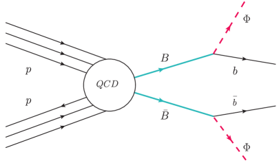
Figure 1: Signal topology

The plan of the paper is as follows. In Section II, we sketch an outline of the extended VLQ models. Section III describes the event-selection criteria and background processes considered in our analysis. Section IV presents the GNN model in detail, along with the design choices we made and the training details. In Section V, we present the HL-LHC reach of the singlet and doublet VLQ models. We conclude the paper in Section VI.

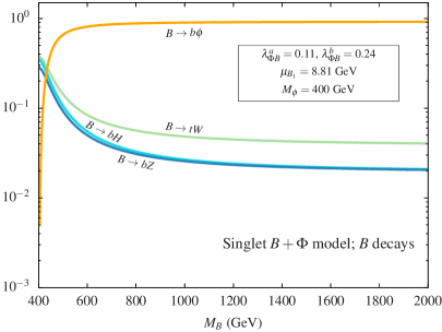
((a))   (a)

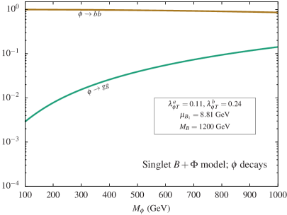
((b))   (b)

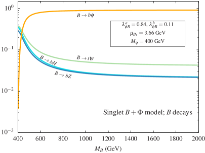
((c))   (c)

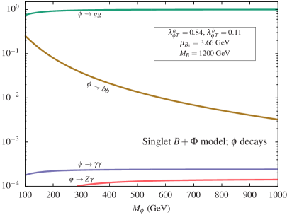
((d))   (d)

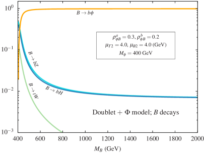
((e))   (e)

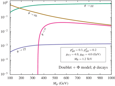
((f))   (f)

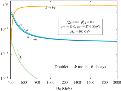
((g))   (g)

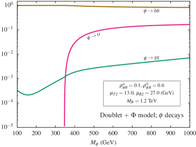
((h))   (h)

Figure 2: Decays of $B$ and $\phi$ in the singlet $B$ [(a)–(d)] and doublet models [(e)–(h)] for some benchmark parameters where $B\to b\phi$ decay dominates over all the other decay modes. On the right panel, we show that either $\phi\to gg$ or $\phi\to b\bar{b}$ can dominate in both scenarios. For more benchmarks and a detailed discussion on the final states from extended VLQ models, see Ref. Bhardwaj et al. (2022a).

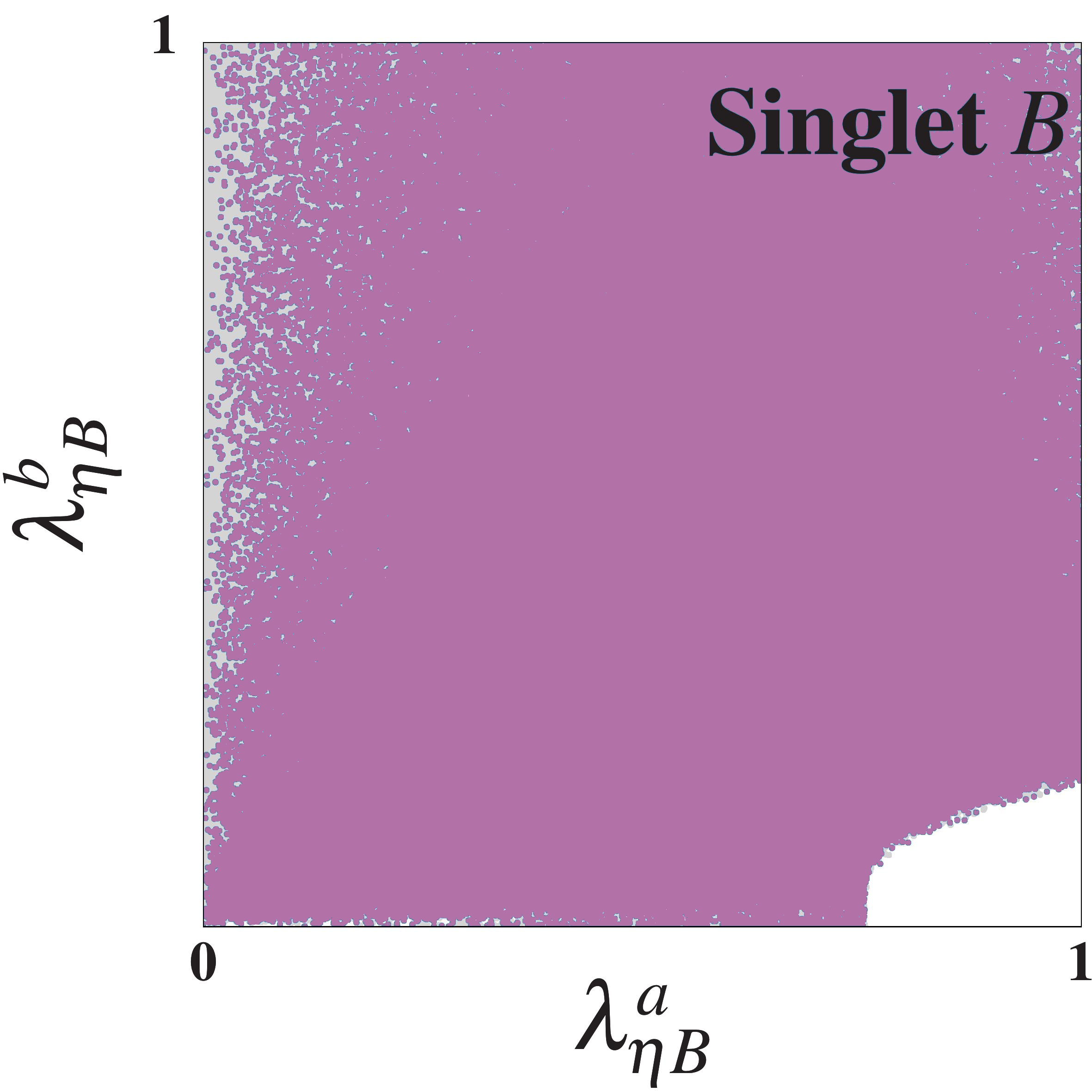
((a))   (a)

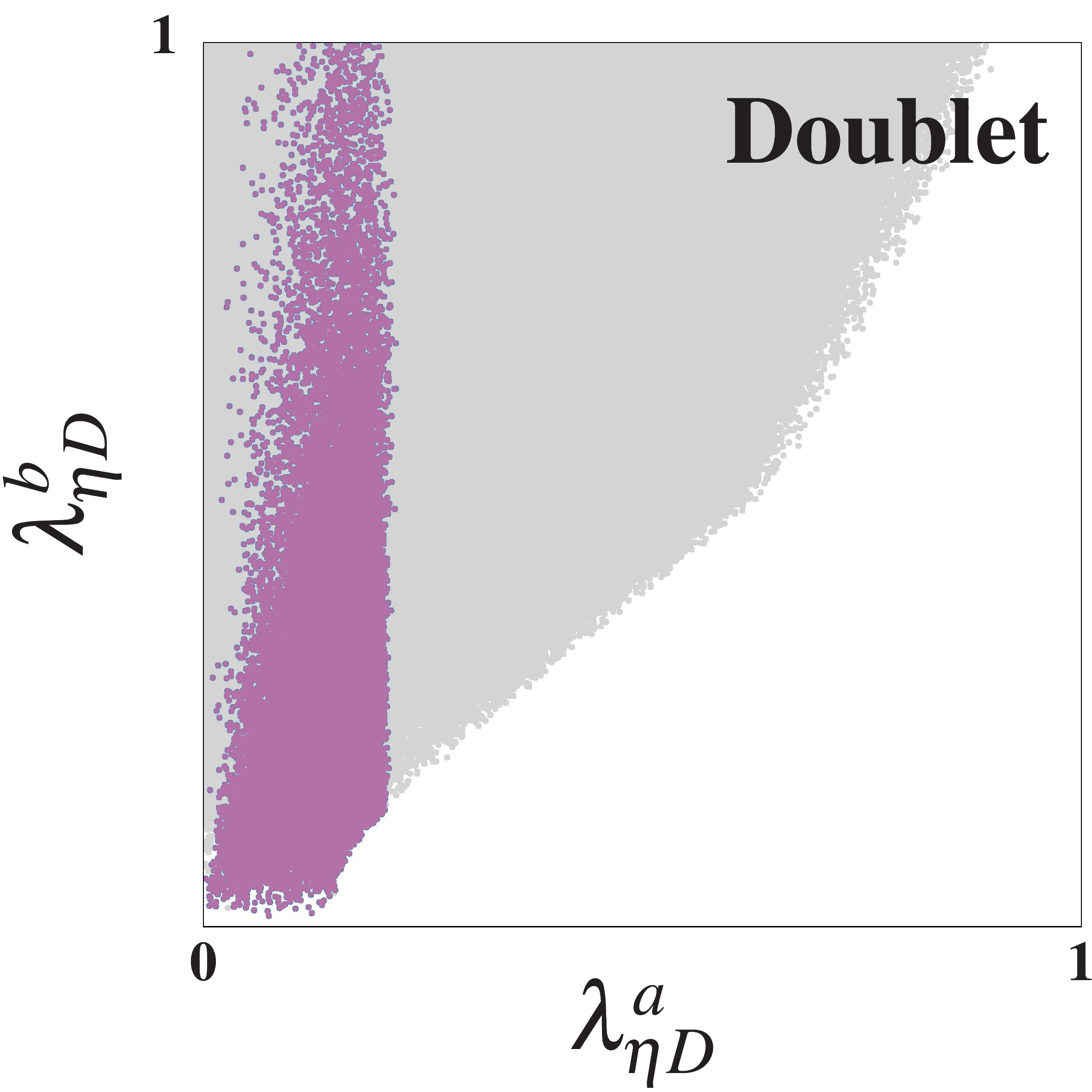
((b))   (b)

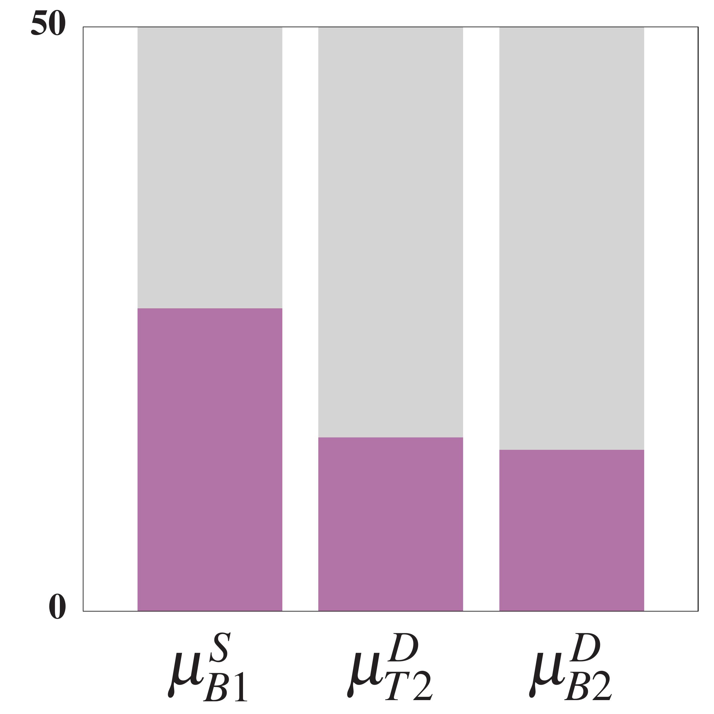
((c))   (c)

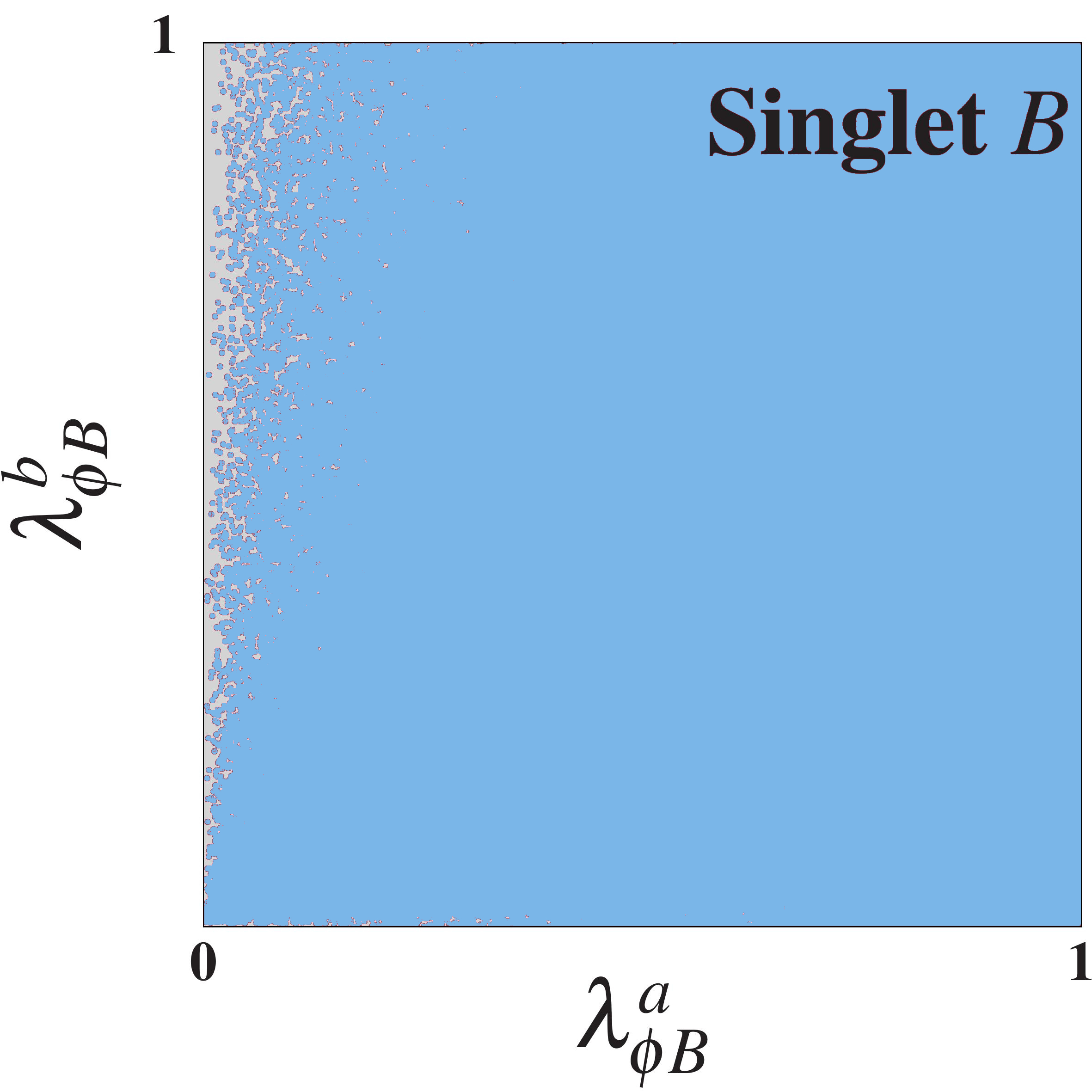
((d))   (d)

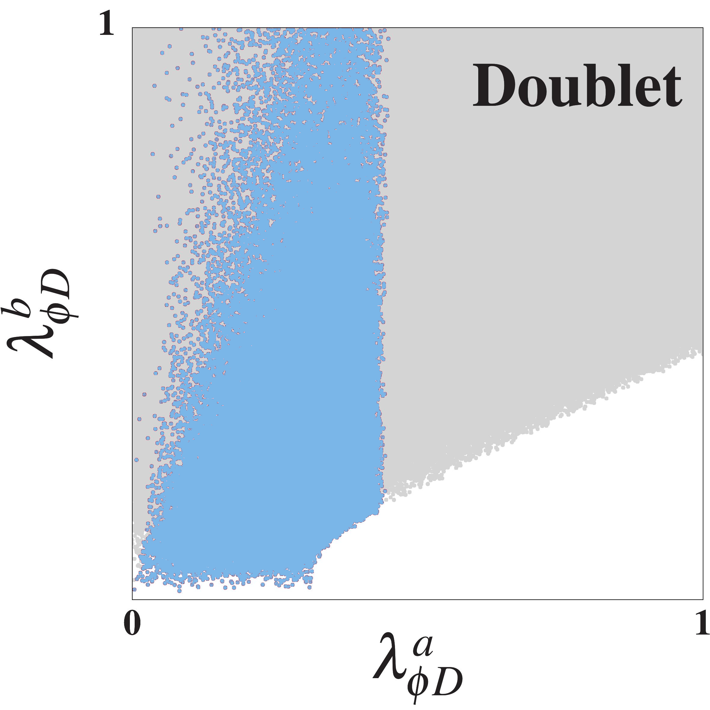
((e))   (e)

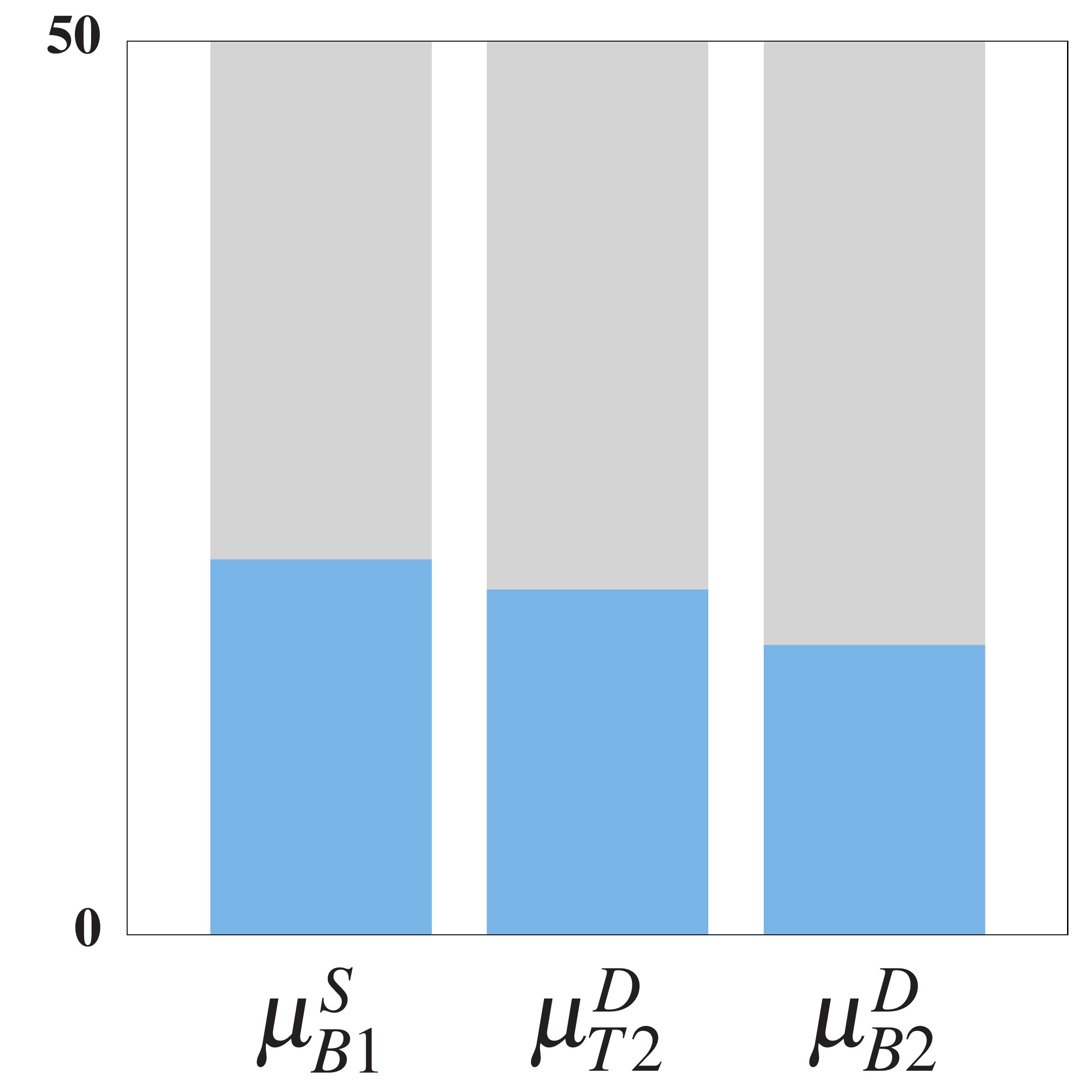
((f))   (f)

Figure 3: Parameter scans for VLQ $B+\>\Phi$ models for benchmark point $\left(M_{B},M_{\Phi}\right)=\left(1.2,0.4\right)$ TeV. The top row [bottom row] shows the scans for a model where the new singlet is a pseudoscalar $\eta$ [scalar $\phi$] boson. The grey-coloured regions are allowed by reinterpreted LHC limits. Coloured in purple [blue] are the regions where BR$(\eta\to gg)\geq 50\%$ [BR$(\phi\to gg)\geq 50\%$].

II Phenomenological Models

We are interested in the following signatures:

$$pp\to B\bar{B}\to\left(b\Phi\right)\>\left(\bar{b}\Phi\right)\to\left\{\begin{array}[]{l}\left(bgg\right)\left(\bar{b}gg\right)\\ \left(bb\bar{b}\right)\left(\bar{b}b\bar{b}\right)\end{array}\right..$$ (3)

Below, we discuss the essential phenomenological parameters in the singlet and doublet $B+\Phi$ models that can produce these processes.

II.1 Singlet $B$ Model

In the notation of Ref. Bhardwaj et al. (2022a), the mass terms relevant to the bottom sector can be written as

$$\mathcal{L}\supset-\Big{\{} \lambda_{b}\left(\bar{Q}_{L}H\right)b_{R}+\omega_{B}\left(\bar{Q}_{L}H\right)B_{R}\$$

$$+M_{B}\bar{B}_{L}B_{R}+h.c.\Big{\}},$$ (4)

where $H=1/\sqrt{2}{\begin{pmatrix}0&v\end{pmatrix}}^{T}$, with $v$ being the vacuum expectation value of the Higgs field, $\lambda_{b}$ is the $b$-quark Yukawa coupling, the off-diagonal $\omega_{B}$ parametrises the mixing between the $b$ and $B$ quarks, and $M_{B}$ is the mass of $B$. Once EWS breaks, we get the mass terms as

$$\mathcal{L}_{mass}=\begin{pmatrix}\bar{b}_{L}&\bar{B}_{L}\end{pmatrix}\begin{pmatrix}\lambda_{b}\frac{v}{\sqrt{2}}&\mu_{B1}\\ 0&M_{B}\end{pmatrix}\begin{pmatrix}b_{R}\\ B_{R}\end{pmatrix}+h.c.,$$ (5)

where $\mu_{B1}=\omega_{B}v/\sqrt{2}$. The matrix is diagonalised by a bi-orthogonal rotation with two mixing angles $\theta_{L}$ and $\theta_{R}$:

$$\begin{pmatrix}b_{L/R}\\ B_{L/R}\end{pmatrix}=\begin{pmatrix}c_{L/R}&s_{L/R}\\ -s_{L/R}&c_{L/R}\end{pmatrix}\begin{pmatrix}b_{1_{L/R}}\\ b_{2_{L/R}}\end{pmatrix},$$ (6)

where $s_{P}=\sin\theta_{P}$ and $c_{P}=\cos\theta_{P}$ for the two chirality projections, and $b_{1}$ and $b_{2}$ are the mass eigenstates. We identify $b_{1}$ as the physical bottom quark and $b_{2}$ is mostly the $B$ quark. Hence, we use the notations $B$ and $b_{2}$ interchangeably.

If we express the $\Phi$ interactions before the breaking of EWS as

$$\mathcal{L}_{int}^{B\Phi}=-\lambda^{a}_{\Phi}\Phi\bar{B}_{L}\Gamma B_{R}-\lambda_{\Phi}^{b}\Phi\bar{B}_{L}\Gamma b_{R}+h.c.,$$ (7)

where $\Gamma=\left\{1,i\gamma_{5}\right\}$ for $\Phi=\left\{\mbox{scalar~}\phi,\mbox{pseudoscalar~}\eta\right\}$, expanding in terms of $b_{1},b_{2}$ we get

$$\mathcal{L}_{int}^{b_{2}\Phi}= -\lambda_{\Phi}^{a}\Phi\left(c_{L}\bar{b}_{2L}-s_{L}\bar{b}_{L}\right)\Gamma\left(c_{R}b_{2R}-s_{R}b_{R}\right)$$

$$-\lambda_{\Phi}^{b}\Phi\left(c_{L}\bar{b}_{2L}-s_{L}\bar{b}_{L}\right)\Gamma\left(c_{R}b_{R}+s_{R}b_{2R}\right)$$

$$+h.c,$$ (8)

after the symmetry breaking. Thus, apart from the masses, the couplings $\lambda_{a}$ and $\lambda_{b}$ and the mixing angles form the set of parameters of the Singlet $B$ model. As explained in Ref. Bhardwaj et al. (2022a), we can draw two types of limits on the VLQ+$\Phi$ models from the current LHC data: 1) We can rescale the current mass exclusion limits on VLQs from their pair-production searches to account for the $\Phi$ decay mode, and 2) recast the heavy resonance searches to put constraints on $\Phi$ production at hadron colliders. The strongest limit on $\Phi$ comes from the clean two-photon search data. (See Refs. Bhardwaj et al. (2022a); Bardhan et al. (2023) for a detailed discussion on the constraints on the VLQ+$\Phi$ models from the LHC data.) Fig. 3 shows different projections of the allowed parameter region after these constraints are considered. The coloured areas are allowed. The dark region is where the loop-mediated $\Phi\to gg$ decay dominates, i.e., BR$(\Phi\to gg)\geq 50\%$, giving a dijet signature at the colliders. In this region, a dedicated collider analysis in fully hadronic modes is necessary to look for VLQ+$\Phi$ models.

II.2 Doublet VLQ

When the $T$ and $B$ quarks together forms a weak doublet, $\mathcal{F}=\left(T\ B\right)^{T}=(\mathbf{3},\mathbf{2},1/6)$, we can write the terms relevant for the quark masses as

$$\mathcal{L}\supset -\lambda_{t}\left(\bar{Q}_{L}\widetilde{H}\right)t_{R}+\rho_{T}\left(\bar{\mathcal{F}}_{L}\widetilde{H}\right)t_{R}+\lambda_{b}\left(\bar{Q}_{L}H\right)b_{R}$$

$$+\rho_{B}\left(\bar{\mathcal{F}}_{L}H\right)b_{R}+M_{F}\bar{\mathcal{F}}_{L}\mathcal{F}_{R}+h.c.$$ (9)

From this, we get the following mass matrices:

$$\mathcal{L}_{mass}^{\mathcal{F}}= \begin{pmatrix}\bar{t}_{L}&\bar{T}_{L}\end{pmatrix}\begin{pmatrix}\begin{array}[]{cc}\lambda_{t}\frac{v}{\sqrt{2}}&0\\ \rho_{T}\,\frac{v}{\sqrt{2}}&M_{T}\end{array}\end{pmatrix}\begin{pmatrix}t_{R}\\ T_{R}\end{pmatrix}$$

$$+\begin{pmatrix}\bar{b}_{L}&\bar{B}_{L}\end{pmatrix}\begin{pmatrix}\begin{array}[]{cc}\lambda_{b}\frac{v}{\sqrt{2}}&0\\ \rho_{B}\,\frac{v}{\sqrt{2}}&M_{B}\end{array}\end{pmatrix}\begin{pmatrix}b_{R}\\ B_{R}\end{pmatrix}+{\textrm{h}.c.}$$ (10)

The interactions between $\Phi$ and the doublet $\mathcal{F}$ can be written as

$$\mathcal{L}_{int}^{\Phi\mathcal{F}}= -\lambda_{\Phi D}^{a}\Phi\,\bar{\mathcal{F}}_{L}\Gamma\mathcal{F}_{R}-\lambda_{\Phi D}^{b}\Phi\,\bar{\mathcal{F}}_{R}\Gamma Q_{L}+h.c.$$ (11)

Expanding, we get the interactions between $\Phi$ and $B$:

$$\mathcal{L}\supset -\lambda_{\Phi D}^{a}\Phi\left(c_{L}^{B}\>\bar{b}_{2L}-s_{L}^{B}\>\bar{b}_{L}\right)\Gamma\left(c_{R}^{B}\>\bar{b}_{2R}-s_{R}^{B}\>\bar{b}_{R}\right)$$

$$+\lambda_{\Phi D}^{b}\Phi\left(c_{R}^{B}\>\bar{b}_{2R}-s_{R}^{B}\>\bar{b}_{R}\right)\Gamma\left(c_{L}^{B}\>\bar{b}_{L}+s_{L}^{B}\>\bar{b}_{2L}\right)+h.c.$$ (12)

In Fig. 2, we show the decays of the $B$ quark and the scalar, $\phi$, for some benchmark choices of parameters where the $B\to b\phi$ decay dominates over all other decay modes and $\phi$ (essentially) decays hadronically. Note that since no fine-tuning is needed to find such parameter points, one can easily find similar benchmarks for the pseudoscalar, $\eta$. Fig. 3 illustrates the dependence of the dominant decay mode of $\Phi$ on the value of the off-diagonal mass term: $\mu_{B1}=\omega_{B}v/\sqrt{2}$, for the singlet model, and $\mu^{D}_{T2}=\mu_{T2}=\rho_{T}\nu/\sqrt{2}$ and $\mu^{D}_{B2}=\mu_{B2}=\rho_{B}\nu/\sqrt{2}$, for the doublet model. The $\Phi\to gg$ mode is enhanced for small mixing values, and the tree-level $\Phi\to b\bar{b}$ mode starts dominating with increasing $\mu_{B1}$. In the doublet mode, $\Phi$ can also decay to a $t\bar{t}$ pair (if kinematically allowed). However, the combined $\Phi\to gg/bb$ mode dominates.

III Collider phenomenology

We use FeynRulesv2.3 Alloul et al. (2014) to obtain the Universal FeynRules Output Degrande et al. (2012) model files, which we use in MadGraph5v3.3 Alwall et al. (2014) to simulate the hard scatterings at the leading order. We use Pythia8 Sjöstrand et al. (2015) for showering and hadronisation, and Delphes3 de Favereau et al. (2014) for simulating a generic LHC detector environment. The events are generated at $\sqrt{s}=14$ TeV. The $b$-tagging efficiency and the mistag rate for the lighter quarks were updated to reflect the Medium working point of the DeepCSV tagger from Ref. Sirunyan et al. (2018). Our analysis relies on two types of jets clustered using the anti-$k_{T}$ algorithm Cacciari et al. (2008) — one with $R=0.4$ (AK4) and the other with $R=1.2$ (fatjet). The AK4 objects are required to pass a minimum-$p_{T}$ cut: $p_{T}>20$ GeV and have $|\eta|<5$. We use the next-to-next-to-leading order (NNLO) signal cross sections from Ref. Sirunyan et al. (2019) (Fig. 4) and for the background processes, we use the highest-order cross sections available in the literature (Table 1). We scan over a wide kinematic range — we take $M_{\Phi}\in\left[300,1000\right]$ GeV and $M_{B}\in\left[1.0,3.0\right]$ TeV.

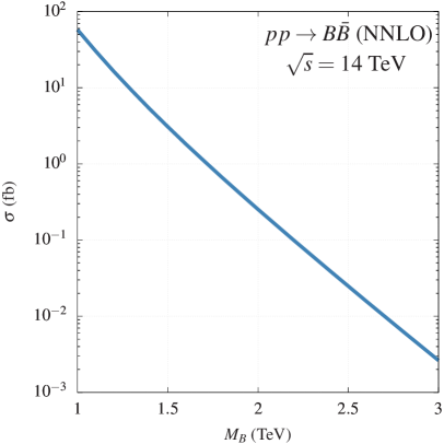
Figure 4: The signal cross section at the $14$ TeV LHC calculated from the leading order cross section as $\sigma$(LO)$\times K_{\rm NNLO}$. We estimate the NNLO QCD $K$-factor to be about $1.3$ from Ref. Sirunyan et al. (2019).

Table 1: Higher-order cross sections of the SM backgrounds considered in our analysis.

Background		$\sigma$	QCD
Processes		(pb)	order
$V$ + jets Balossini et al. (2010); Catani et al. (2009)	$W$ + jets	$1.95\times 10^{5}$	NLO
	$Z$ + jets	$6.33\times 10^{4}$	NNLO
$tt$ Muselli et al. (2015)	$tt$ + jets	$988.57$	N3LO
Single $t$ Kidonakis (2015)	$tW$	$83.10$	N2LO
	$tb$	$248.00$	N2LO
	$t$ + jets	$12.35$	N2LO
$VV$ + jets Campbell et al. (2011)	$WW$ + jets	$124.31$	NLO
	$WZ$ + jets	$51.82$	NLO
$VH$ Cepeda et al. (2019)	$WH$	$1.50$	NNLO (NLO EW)
	$ZH$	$0.98$	NNLO (NLO EW)
$ttV$ Kulesza et al. (2019); de Florian et al. (2016)	$ttZ$	$1.05$	NLO + NNLL
	$ttW$	$0.65$	NLO + NNLL
	$ttH$	$0.61$	NLO

III.1 The background and selection criteria

Our signal has at least two $b$ jets and two $\Phi$ (fat)jets originating in heavy particles, but no isolated leptons. We collect all the major background processes that could lead to similar final states in Table 1. With the signal topology in mind, we first pass the events through the following selection criteria:

• $\ell$-veto, where $l\in\{e,\mu\}$ and $H_{T}$ > 1 TeV.

  We require an event to have no electrons or muons, and the scalar sum of hadronic transverse momenta ($H_{T}$) should be at least $1$ TeV.

• At least three AK4 jets with $p_{T1},~p_{T2}>100$ GeV and $p_{T3},\ldots,p_{Tn}>30$ GeV.

  In our analysis, we only consider reconstructed jets with a minimum $p_{T}$ of $30$ GeV. We also demand the $p_{T}$ of the top two leading-$p_{T}$ jets should be at least $100$ GeV.

• At least two AK4 jets in the event must be b-tagged.

• At least one fatjet $(R=1.2)$ with $p_{T}>200$ GeV

  We tag one of the $\Phi$-jets in the event as a fatjet of $R=1.2$ with minimum $p_{T}>200$ GeV. We also demand that the mass of fatjet, $M_{J}>250$ GeV. To cover both $\Phi\to gg/bb$, our analysis relies only on the two-pronged nature of $\Phi$.

• At least two b-tagged jets with $\Delta R_{b_{i}J}\geq 1.2$.

  We demand that the event has at least two b-tagged jets that are well-separated from the fatjet, i.e., they do not come from the $\Phi$.

The strong $p_{T}$ cuts and the demand for $b$-tagged jets essentially eliminate the QCD multijet background. These topology-motivated cuts also reduce the total background from other processes significantly (roughly by an order of magnitude) while retaining a large part of the signal. We can see the reduction in Table 2. Fig. 5 shows the efficiency of the selection cuts at different parameter points. However, as expected, the set of background events remains overwhelmingly larger in this hadronic channel even after the cuts. We collect all the signal and background events that pass the selection cuts and feed them to a GNN model for further analysis.

Table 2: Cut flow for the three benchmark choices of the signal and the relevant background processes. We use the MLM jet-parton shower matching technique Mangano et al. (2007) to generate the background samples as indicated by the additional jets in brackets. Wherever necessary, we simulate background events with generation-level cuts to reduce computational time. The events are estimated for luminosity $\mathcal{L}=3$ ab^-1.

	Selection Criteria
	$\mathfrak{C}_{1}$	$\mathfrak{C}_{2}$	$\mathfrak{C}_{3}$	$\mathfrak{C}_{4}$	$\mathfrak{C}_{5}$
Signal benchmarks
$M_{B}=1200$ GeV, $M_{\Phi}=400$ GeV	$4.90\text{\times}{10}^{4}$	$4.90\text{\times}{10}^{4}$	$4.76\text{\times}{10}^{4}$	$3.76\text{\times}{10}^{4}$	$3.22\text{\times}{10}^{4}$
$M_{B}=1200$ GeV, $M_{\Phi}=900$ GeV	$4.91\text{\times}{10}^{4}$	$4.91\text{\times}{10}^{4}$	$4.78\text{\times}{10}^{4}$	$3.90\text{\times}{10}^{4}$	$3.35\text{\times}{10}^{4}$
$M_{B}=2000$ GeV, $M_{\Phi}=700$ GeV	$754$	$754$	$725$	$664$	$571$
$M_{B}=2800$ GeV, $M_{\Phi}=400$ GeV	$19$	$19$	$18$	$18$	$14$
Background processes
$t_{h}t_{h}~(+j)$	$2.21\text{\times}{10}^{7}$	$2.21\text{\times}{10}^{7}$	$1.22\text{\times}{10}^{7}$	$4.504\text{\times}{10}^{6}$	$1.38\text{\times}{10}^{6}$
$Z_{bb}~(+j)$	$1.36\text{\times}{10}^{7}$	$1.18\text{\times}{10}^{7}$	$2.54\text{\times}{10}^{6}$	$4.11\text{\times}{10}^{5}$	$1.45\text{\times}{10}^{5}$
$tb~(+j)$	$4.28\text{\times}{10}^{5}$	$4.14\text{\times}{10}^{5}$	$2.20\text{\times}{10}^{5}$	$6.21\text{\times}{10}^{4}$	$1.44\text{\times}{10}^{4}$
$t_{h}t_{h}H~(+j)$	$5.50\text{\times}{10}^{4}$	$5.50\text{\times}{10}^{4}$	$4.74\text{\times}{10}^{4}$	$2.40\text{\times}{10}^{4}$	$1.13\text{\times}{10}^{4}$
$W_{h}~(+j)$	$8.34\text{\times}{10}^{6}$	$7.09\text{\times}{10}^{6}$	$1.85\text{\times}{10}^{5}$	$3.98\text{\times}{10}^{4}$	$8.74\text{\times}{10}^{3}$
$t_{h}t_{h}W_{h}~(+j)$	$7.15\text{\times}{10}^{4}$	$7.15\text{\times}{10}^{4}$	$3.97\text{\times}{10}^{4}$	$1.84\text{\times}{10}^{4}$	$6.67\text{\times}{10}^{3}$
$W_{h}Z_{bb}~(+j)$	$1.84\text{\times}{10}^{5}$	$1.81\text{\times}{10}^{5}$	$6.24\text{\times}{10}^{4}$	$2.13\text{\times}{10}^{4}$	$5.39\text{\times}{10}^{3}$
$t_{h}t_{h}Z_{h}~(+j)$	$4.58\text{\times}{10}^{4}$	$4.57\text{\times}{10}^{4}$	$2.83\text{\times}{10}^{4}$	$1.28\text{\times}{10}^{4}$	$5.17\text{\times}{10}^{3}$
$h_{b}W_{h}~(+j)$	$6.77\text{\times}{10}^{3}$	$98$	$<10$	$<10$	$<10$
$h_{b}Z_{h}~(+j)$	$4.31\text{\times}{10}^{3}$	$66$	$<10$	$<10$	$<10$
		Total number of background events:			$1.58\text{\times}{10}^{6}$

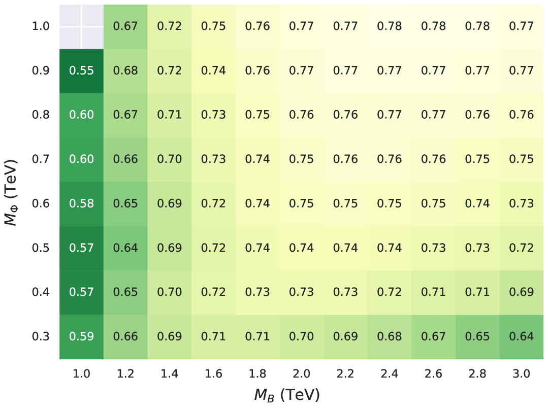
Figure 5: Selection efficiency after $\mathfrak{C}_{5}$ at various parameter points on the $M_{B}-M_{\Phi}$ plane. On average, the efficiency exceeds $70\%$.

IV The Graph Neural Network Model

GNNs are a class of permutation-invariant machine learning methods that learn functions on graphs. The functions may be at the node, edge, or graph levels. The workings of GNNs are better understood by thinking of them as message-passing frameworks: GNN modules (layers) pass messages (information) between nodes to let each node learn the embedding that depends on its attributes and its connections to other nodes in the graph. It can be mathematically expressed as Shlomi et al. (2020),

$$\hskip-5.0pt\mathbf{x}_{i}^{(k)}=\gamma^{(k)}\Big{(}\mathbf{x}_{i}^{(k-1)},\bigoplus_{j\in\mathcal{N}(i)}\phi^{(k)}\big{(}\mathbf{x}_{i}^{(k-1)},\mathbf{x}_{j}^{(k-1)},\mathbf{e}_{j,i}\big{)}\Big{)},$$ (13)

where $\mathbf{x}_{i}^{(k)}$ denotes the embedding of the $i$th node at the $k$th layer of the GNN, $\mathcal{N}(i)$ is the neighbourhood of $i$, $e_{j,i}$ is the edge (link) from node $j$ to node $i$, $\bigoplus$ denotes a differentiable, permutation invariant function such as sum, max and min, and $\gamma$ and $\phi$ are differentiable functions like multilayer perceptrons. For graph-level tasks (like our classification task), the latent embeddings of each node are aggregated through a permutation-invariant function to give a single prediction. GNNs can be helpful for tasks such as particle tracking and particle flow Kieseler (2020), jet identification Qu and Gouskos (2020); Mikuni and Canelli (2020), and, in particular, event identification Abdughani et al. (2021); Choma et al. (2018); Abbasi et al. (2022). GNNs are especially effective since they operate much lower than boosted decision trees and deep neural networks (DNNs), allowing them to model features that might be difficult for us to construct or provide. (See Ref. Shlomi et al. (2020) for a comprehensive review of GNNs.)

IV.1 Constructing graphs from a collision event

Even though our event selection criteria focus on three AK4 jets (of which at least two are $b$ jets) and one fatjet, a typical signal event contains more well-defined objects due to the high jet multiplicity of the $B$-quark decay. In principle, once an event passes our selection criteria, all well-defined objects in that event can be used to classify the event using a GNN model. We can also make use of the event-level features. Therefore, to capture the information content in the events, we model them as heterogeneous graphs.

We represent the kinematic features of jets and fatjets with special abstract nodes — we call them ‘shared attributes’ or SA nodes — essentially containing a set of attributes: $\eta$, $\phi$, $m$, and $p_{T}$. By constructing an abstract common node type for these kinematic features, we enable the model to process these generic features in a unified way and learn functions to model them better. Each jet or fatjet in a selected event has one corresponding SA node. Since our event topology has two kinds of hadronic objects (jets and fatjets), we choose two kinds of auxiliary nodes to represent them. The auxiliary jet node contains features like $b$ tag, MeanSqDeltaR (the mean of $p_{T}^{2}$-weighted RMS distance between the constituent and the jet axis), and PTD (a measure of the $p_{T}$ dispersion of the jet constituents). The auxiliary fatjet node has $N$-subjettiness ratios and girth (mean of the $p_{T}$-weighted distances of the constituents from the fatjet axis) along with their four-momenta as its attributes.

The graph also contains two additional nodes — global and CLS. The global node contains features of the whole event, such as $H_{T}$ and $\not{E}_{T}$. The CLS node extracts the embedding for the entire graph (i.e., event) as a vector. This vector is then fed as the input to a fully connected DNN that performs the signal vs. background binary classification. Table 3 lists the attribute content of each node type we construct. For simplicity, we do not specify edge-level attributes and instead let the GNN module learn these from the node features.

Sequential graph contruction: We sequentially construct the event graph — Fig. 6 illustrates the construction.

1. GNN layer 1-2: In the first step, the SA nodes are connected with each other (i.e., a clique graph) to enable global interactions among the kinematics of the reconstructed objects and to ensure that each subsequent connection has some information about other nodes present at the global scale. We then perform a round of message passing.

2. GNN layer 2-3: Each SA node is connected to its corresponding auxiliary jet or fatjet node in the second step. This allows for object-specific embedding learning, where the kinematic information gathered from the previous layer and the node-level input from the current one are used to construct meaningful embeddings for each reconstructed object. A round of message passing is performed after the connection is made.

3. GNN layer 3-5: Jets and fatjets located nearby are likely related. For instance, a fatjet will be close to its constituent jets. Furthermore, independent jets with a common parent are also likely to be close. To incorporate this, we connect nodes to their nearest objects in the $\eta-\phi$ plane in the next step using the $k$ Nearest Neighbours ($k$NN) algorithm. We also connect the global node of the jet and fatjet nodes using a bidirectional link. We do this for two reasons — we want to provide event-level information to each (fat)jet, and we also want to enable long-range interactions between distant jets, as this information transfer can occur through the global node. This choice is critical for large graphs, and similar strategies have been employed previously Hussain et al. (2021); Hwang et al. (2022). Once the connections are in place, we perform two rounds of message passing.

4. GNN layer 5-6: Once all message passings are performed, and each node has an appropriate embedding, we connect all the nodes to the CLS token/node to extract the graph-level class information and perform a round of message passing. This idea is commonly used in Transformers in language-related tasks Devlin et al. (2018).

We primarily use the GATv2Conv Brody et al. (2021) message-passing module to construct our GNN as it shows superior performance over other methods such as GCNConv Veličković et al. (2017) and SAGEConv Hamilton et al. (2017). This performance improvement could be attributed to the attention mechanism employed by the GNN. The GATv2Conv module incorporates the attention mechanism to learn an embedding for a node by selectively attending to information obtained by its neighbours,

$$\mathbf{x}^{\prime}_{i}=\sum_{j\in\mathcal{N}(i)\cup\{i\}}\alpha_{i,j}\mathbf{\Theta}_{t}\mathbf{x}_{j},$$ (14)

where the attention coefficients $\alpha_{i,j}$ are computed as

$$\alpha_{i,j}=\frac{\exp\left(\mathbf{a}^{\top}\mathrm{LeakyReLU}\left(\mathbf{\Theta}_{s}\mathbf{x}_{i}+\mathbf{\Theta}_{t}\mathbf{x}_{j}\right)\right)}{\sum_{k\in\mathcal{N}(i)\cup\{i\}}\exp\left(\mathbf{a}^{\top}\mathrm{LeakyReLU}\left(\mathbf{\Theta}_{s}\mathbf{x}_{i}+\mathbf{\Theta}_{t}\mathbf{x}_{k}\right)\right)}.$$ (15)

Here, subscripts $s$ and $t$ indicate the source and the target in the message passing framework, and $\mathbf{\Theta}_{s,t}$ are their corresponding parameters. Using the constructed event embeddings from CLS node, we use a simple, fully connected deep neural network (DNN) to perform the final event classification.

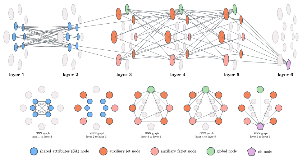
Figure 6: Constructing the GNN: We show sequential construction of the graph along with flow of information (message passing) in the GNN model. We use GATv2Conv layer to implement the message passing operation in layer.

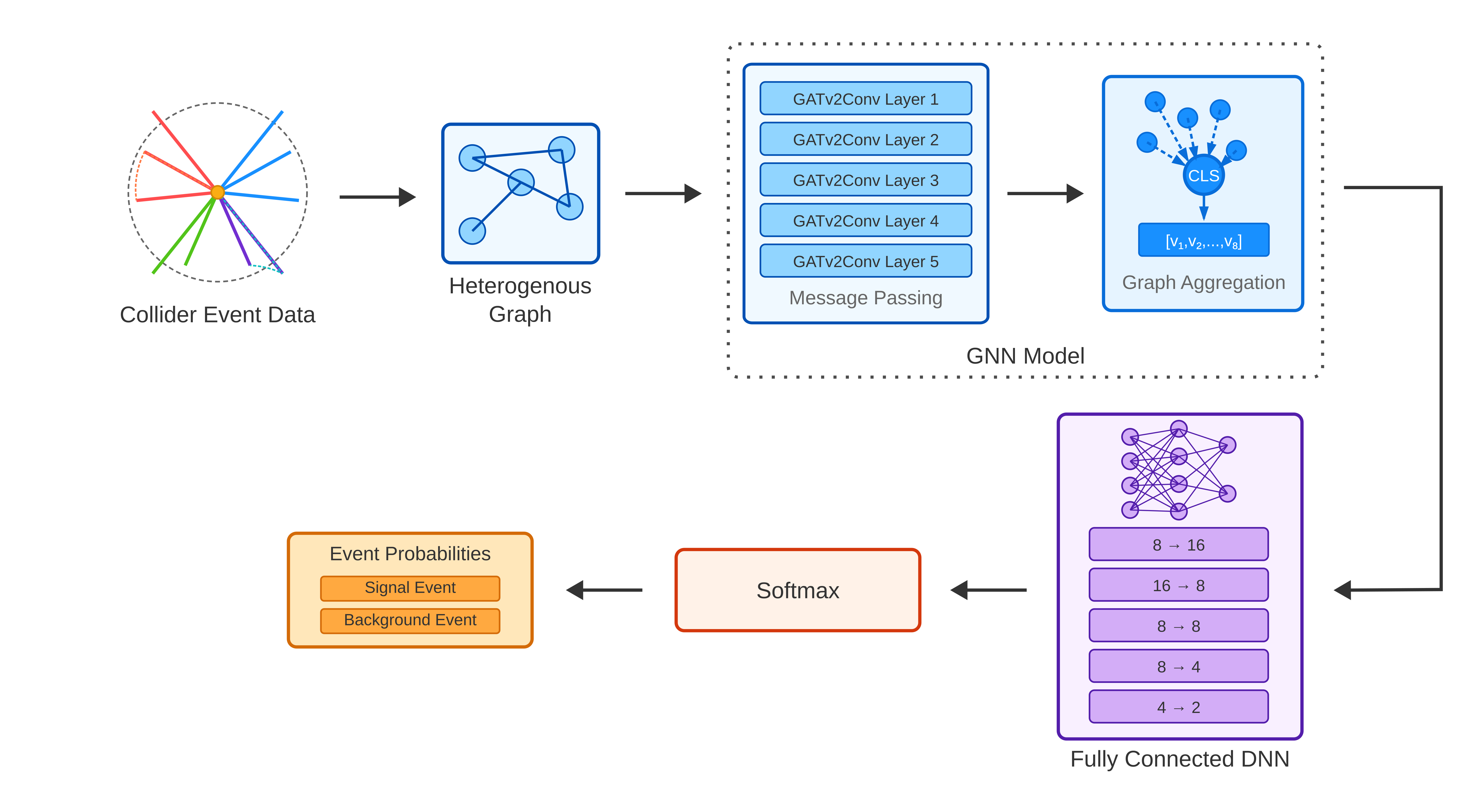
Figure 7: Schematic of the event classification pipeline. We perform an event-level signal vs. background classification on the learned event embeddings using a DNN model. We use a GNN model (Fig. 6) to learn the embeddings of the event.

Node-type	Input Features
Shared attributes (SA) nodes	$m,p_{T},\eta,\phi$
Auxiliary jet	MeanSqDeltaR, $b$-tag, PTD
Auxiliary fatjet	girth, $E,p_{x},p_{y},p_{z},\tau_{i},\tau_{ij}$
global	$H_{T},\not{E}_{T}$
CLS	–

Table 3: Node types and their respective input features. For the auxiliary fatjet node, $\tau$ denotes the $N$-subjettiness feature, where $i=1,2,3,4$ and $\tau_{ij}$ denotes the $N$-subjettiness ratios ($j=1,2,3$).

IV.2 Classifier description and hyperparameters tuning

Our classifier has two components: a GNN model (with six graph-convolution layers) to learn the event embedding and a DNN model (with five fully connected layers) for event classification using the embeddings. Fig. 7 shows a representative diagram of the classification pipeline. We use BatchNorm Ioffe and Szegedy (2015) and Dropout Srivastava et al. (2014) layers to regularise our model with dropout probability $p=0.5$. We use the AdamW optimiser Loshchilov and Hutter (2017) with a weight decay value of $\lambda=10^{-4}$. We run a comprehensive hyperparameter search on the depth of the model (both GNN and DNN), the sizes of the various nodes of the different layers, the regularisation parameters, the learning rate and weight decay, the batch size, the number of epochs of training, and the value of $k$ for $k$NN for generating the graph. Our hyperparameters are optimised using the Bayesian Search strategy on Weights and Biases Biewald (2020).

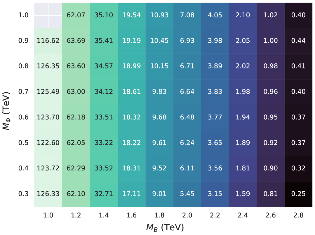
Figure 8: Discovery sensitivity [defined in Eq. (18)] obtained from the GNN+DNN model for each parameter point on the $M_{B}-M_{\Phi}$ grid considered in Fig. 5.

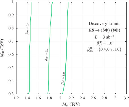
((a))   (a)

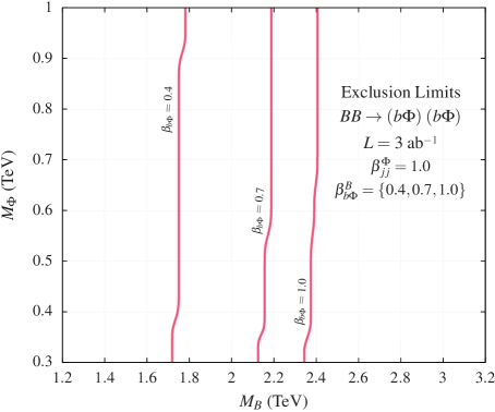
((b))   (b)

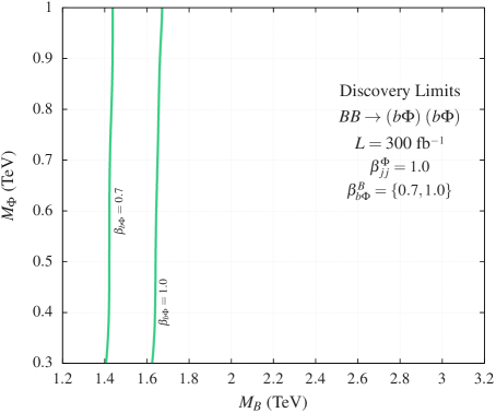
((c))   (c)

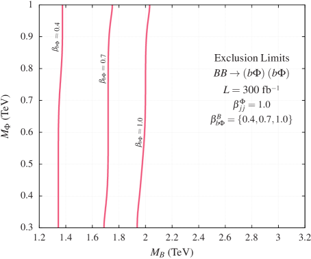
((d))   (c)

Figure 9: LHC reach plots for $BB\to\left(b\Phi\right)\>\left(b\Phi\right)$ signal at the HL-LHC, i.e., for luminosity, $L=3000$ fb^-1 [(a) and (b)]. The left panel shows the $\mathcal{Z}_{D}=5$ [discovery, Eq. (18)] contours and the right panel shows the $\mathcal{Z}_{E}=2$ [$\sim$ exclusion, Eq. (19)] contours for three different values of branching in the $B\to b\Phi$ mode: $\beta_{b\Phi}=40\%,70\%,100\%$. The boson, $\Phi$, has a two-prong decay to either a pair of $b$-jets or gluon jets. We also show these plots for $L=300$ fb^-1 in (c) and (d).

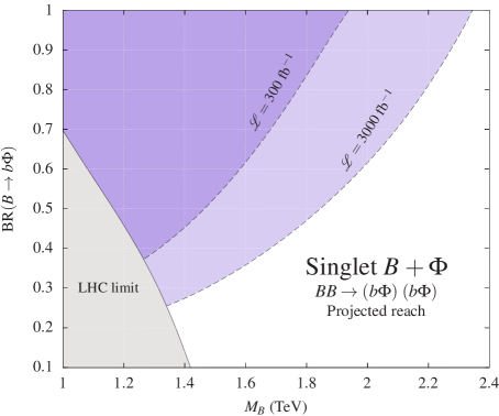
((a))   (a)

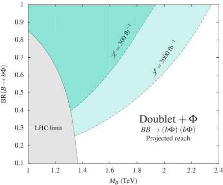
((b))   (b)

Figure 10: Projected LHC reach for (a) the Singlet $B+\Phi$ model and (b) the Doublet $+\Phi$ in the proposed channel along with the regions ruled out from the current LHC data (in grey) for $L=300$ and $3000$ fb^-1.

IV.3 Training Strategy

We train the classifier with a two-step strategy:

1. Pre-training: We pre-train our model on all signal parameter points we consider.

2. Finetuning: After pre-training the classifier, we finetune our model on each mass point.

Our strategy is mainly motivated by the mounting evidence that large models trained on vast amounts of data generalise better than specific models Li et al. (2024); Touvron et al. (2023); Reid et al. (2024); Brown et al. (2020). Models trained on larger datasets are better able to capture the underlying properties.

Our signal is characterised by $M_{B}$ and $M_{\Phi}$. We treat the branching ratio of $B$ to the new mode, i.e., BR$(B\to b\Phi)$, as a free parameter that controls the yield of the signal. As mentioned earlier, we pick eight benchmark values for $M_{\Phi}$ (from $300$ GeV to $1$ TeV, sampled at an interval of $100$ GeV), and eleven values for $M_{B}$ ($1$ TeV to $3$ TeV, sampled at an interval of $200$ GeV). Considering all combinations leaves us with $87$ distinct parameter points (the parameter point $M_{B}=M_{\Phi}=1$ TeV is kinematically forbidden) to pre-train the model on. The model is trained to perform binary classification at these parameter points.

Loss calculation: We train an unbiased signal vs background classifier in our pre-training stage, i.e., we set the total background weight equal to the total signal weight. For this, we weigh the background processes such that the total background weight is the proportionate sum of the rates (cross-sections). Therefore, the weight of a particular background process is,

$$w_{b_{i}}\propto\frac{\sigma_{b_{i}}}{N_{b_{i}}},$$ (16)

where $\sigma_{b_{i}}$ is the cross-section of the background process $i$ and $N_{b_{i}}$ is the number of samples of background process $i$ in the dataset. Similarly, we weigh the signal events. However, since the signal cross-section varies across the parameter range we scan, we ensure that all points contribute equally to the final loss by setting the weights as

$$w_{s}\propto\frac{1}{N_{s}},$$ (17)

where $N_{s}$ is the number of signal samples for a parameter point. As we showed earlier Bardhan et al. (2023), a bias-adjusted loss function performs better than the conventional cross-entropy loss. We find that such a loss function effectively balances the performance across all the signal parameter points while cutting out heavy background processes in the current case as well.

Finetuning: While finetuning to a particular parameter point, we keep the GNN model frozen and retrain only the fully connected DNN. Each parameter point is finetuned independently, giving us $87$ models in total. We scan the threshold values of the classifier response curve and select the best value that maximises the discovery sensitivity Cowan et al. (2011), given as

$$\mathcal{Z}_{D}=\sqrt{2(N_{S}+N_{B})\ln\left(\frac{N_{S}+N_{B}}{N_{B}}\right)-2N_{S}},$$ (18)

where $N_{S}$ and $N_{B}$ are the number of surviving signal and background events at the HL-LHC, respectively. We take the branching ratio in the new mode $\beta_{b\Phi}=1$. The pre-trained generic model performs well on most parameter points, as seen in Fig. 8. Finetuning shows a modest improvement in the final $\mathcal{Z}_{D}$ score, with noticeable improvements at the extremums of the parameter points.

V Prospects

Fig. 10 shows the LHC reach obtained using the finetuned GNN model for two different projected luminosities, $\mathcal{L}=3000$ fb^-1 [Figs. (a) and (b) in Fig. 10] and $300$ fb^-1 [Figs. (c) and (d) in Fig. 10]. We show the $5\sigma$ (discovery) and $2\sigma$ ($\sim$ exclusion) contours on the $M_{B}-M_{\Phi}$ plane with different contours corresponding to different values of $\beta_{b\Phi}$. Since the number of signal events scales with the branching ratio as $\beta_{b\Phi}^{2}$, these contours can be easily interpreted for other scenarios (e.g., when the standard decay modes dominate or the $B$ quark has additional decay modes) as well by scaling down the $\beta_{b\Phi}=1.0$ line appropriately. We estimate the discovery contours with the $Z_{D}$ score [Eq. (18)], and the exclusion limits with Cowan et al. (2011),

$$\mathcal{Z}_{E}=\sqrt{2N_{S}-2N_{B}\ln\left(\frac{N_{S}+N_{B}}{N_{B}}\right)},$$ (19)

where $N_{S},N_{B}$ are the number of surviving signal and background events at the LHC, respectively. In general, we see that with the complex GNN model, it is possible to attain a discovery significance score of $5\sigma$ at values $M_{B}>2$ TeV. The reach is only slightly better towards the higher end of $M_{\Phi}$ considered due to the lower boost of $\Phi$-jet; overall, the GNN+DNN model efficiency follows the same trend as Fig. 5.

As expected, the LHC can exclude regions beyond its discovery reach. The projected exclusion limits apply to both the singlet $B+\Phi$ and doublet $+\>\Phi$ models. Since the contours in Fig. 10 are insensitive to $M_{\Phi}$, we reinterpret the exclusion contours and plot them on the BR$(B\to b\Phi)$ vs. $M_{B}$ plane in Fig. 10 by picking the maximum value $M_{B}$ allowed at the $2\sigma$ level for each BR$(B\to b\Phi)$ value $\in\left[0.1,1.0\right]$. The purple (turquoise) regions are excludable in the singlet $B+\Phi$ (doublet $+\>\Phi$) model. The current limits (recast from the LHC data for $L=139$ fb^-1) are coloured in grey. The gain is considerable, particularly at the HL-LHC. It also extends beyond the HL-LHC limits for the monoleptonic final states, as obtained in our previous paper Bardhan et al. (2023). There, the singlet $B\>+\>\Phi$ exclusion limit stood at $M_{B}=1.8$ TeV, for BR$(B\to b\Phi)=50\%$, corresponding to the maximal signal yield.

VI Conclusions

In this paper, we studied the pair production of vectorlike bottom-type quarks ($B$), with each decaying to a $b$ quark and a new gauge-singlet scalar or pseudoscalar boson $\Phi$ that dominantly decays to $gg$ or $b\bar{b}$ pairs. Such final states ($2b+4j$ or $6b$) are difficult to isolate due to the absence of any leptonic handles and an overwhelmingly large hadronic background at the LHC. We designed a sophisticated GNN model-based event classification pipeline to tag the resulting fully hadronic final states. By representing collision events as heterogeneous graphs containing jets, fatjets, and global event features, our model utilised the permutation invariance and message-passing strengths of GNNs. We also employed a novel two-step training strategy to train our event classifier: a pre-training over the entire set of benchmark parameter points before fine-tuning the model for classification at a particular parameter point. This strategy closely follows the one used to train large foundation models in various domains (see, e.g., Refs. Li et al. (2024); Touvron et al. (2023); Reid et al. (2024); Brown et al. (2020)). Our estimation showed that, at the HL-LHC ($L=3000$ fb^-1), $M_{B}$ up to $2.4$ TeV could be excluded by a dedicated search in the joint $2b+4j/6b$ channel for BR$(B\to b\Phi)\approx 100\%$. Even for a moderate BR in the new mode, $\beta_{b\Phi}=0.4$, the exclusion limit in $M_{B}$ goes up to about $1.8$ TeV. Our projections indicate that, in the future, the LHC sensitivity to the singlet and doublet VLQ scenarios (see Fig. 10) could be significantly enhanced, particularly in regions of parameter space currently unconstrained. Thus, a dedicated search for pair-produced VLQs decaying through the $4j+2b\>/\>6b$ channel could uncover or constrain a wide range of new physics scenarios.

Though our analysis is thorough, a more rigorous analysis with real data, higher-order simulations, or better simulation of detector effects (e.g., with Geant4 Agostinelli et al. (2003)) could improve our results. Our estimations can be taken as conservative since, in the signal, we only included events where each pair-produced $B$ quark decayed to a $b$ and a $\Phi$ pair. Including hadronic final states from all pair-production signatures arising from standard decays of the $B$ quark (i.e., $B\to\left\{tW,bZ,bh\right\}$) that satisfy our selection criteria could enhance the signal strength, as we showed in Ref. Bardhan et al. (2023) while studying the prospects of an inclusive $tW+X$ signal arising from the decays of pair-produced $B$ quarks. Moreover, as Refs. Mandal and Mitra (2013); Mandal et al. (2015) showed, accounting for contaminating contributions from other production processes (e.g., single productions) could lead to further enhancement of the sensitivities. This is interesting because, beyond $2$ TeV, the pair production process may not remain the leading production process of VLQs. Moreover, non-conventional single productions ($pp\to B\Phi$) also come into play in that regime.

Model Files

The Universal FeynRules Output Degrande et al. (2012) files used in our analysis are available at https://github.com/rsrchtsm/vectorlikequarks/ under the name SingBplusPhi.

References

- Gopalakrishna et al. (2011) Shrihari Gopalakrishna, Tanumoy Mandal, Subhadip Mitra, and Rakesh Tibrewala, “LHC Signatures of a Vector-like b’,” Phys. Rev. D 84, 055001 (2011), arXiv:1107.4306 [hep-ph] .
- Gopalakrishna et al. (2014) Shrihari Gopalakrishna, Tanumoy Mandal, Subhadip Mitra, and Grégory Moreau, “LHC Signatures of Warped-space Vectorlike Quarks,” JHEP 08, 079 (2014), arXiv:1306.2656 [hep-ph] .
- Alves et al. (2024) João M. Alves, G. C. Branco, A. L. Cherchiglia, C. C. Nishi, J. T. Penedo, Pedro M. F. Pereira, M. N. Rebelo, and J. I. Silva-Marcos, “Vector-like singlet quarks: A roadmap,” Phys. Rept. 1057, 1–69 (2024), arXiv:2304.10561 [hep-ph] .
- Arhrib et al. (2018) A. Arhrib, R. Benbrik, S. J. D. King, B. Manaut, S. Moretti, and C. S. Un, “Phenomenology of 2HDM with vectorlike quarks,” Phys. Rev. D 97, 095015 (2018), arXiv:1607.08517 [hep-ph] .
- Han et al. (2019) Huayong Han, Li Huang, Teng Ma, Jing Shu, Tim M. P. Tait, and Yongcheng Wu, “Six Top Messages of New Physics at the LHC,” JHEP 10, 008 (2019), arXiv:1812.11286 [hep-ph] .
- Bizot et al. (2018) Nicolas Bizot, Giacomo Cacciapaglia, and Thomas Flacke, “Common exotic decays of top partners,” JHEP 06, 065 (2018), arXiv:1803.00021 [hep-ph] .
- Benbrik et al. (2020) Rachid Benbrik et al., “Signatures of vector-like top partners decaying into new neutral scalar or pseudoscalar bosons,” JHEP 05, 028 (2020), arXiv:1907.05929 [hep-ph] .
- Cacciapaglia et al. (2019a) Giacomo Cacciapaglia, Gabriele Ferretti, Thomas Flacke, and Hugo Serôdio, “Light scalars in composite Higgs models,” Front. in Phys. 7, 22 (2019a), arXiv:1902.06890 [hep-ph] .
- Aguilar-Saavedra et al. (2020) J. A. Aguilar-Saavedra, J. Alonso-González, L. Merlo, and J. M. No, “Exotic vectorlike quark phenomenology in the minimal linear model,” Phys. Rev. D 101, 035015 (2020), arXiv:1911.10202 [hep-ph] .
- Cacciapaglia et al. (2019b) Giacomo Cacciapaglia, Thomas Flacke, Myeonghun Park, and Mengchao Zhang, “Exotic decays of top partners: mind the search gap,” Phys. Lett. B 798, 135015 (2019b), arXiv:1908.07524 [hep-ph] .
- Wang et al. (2021) Daohan Wang, Lei Wu, and Mengchao Zhang, “Hunting for top partner with a new signature at the LHC,” Phys. Rev. D 103, 115017 (2021), arXiv:2007.09722 [hep-ph] .
- Banerjee et al. (2022a) Avik Banerjee et al., “Phenomenological aspects of composite Higgs scenarios: exotic scalars and vector-like quarks,” (2022a), arXiv:2203.07270 [hep-ph] .
- Banerjee et al. (2022b) Avik Banerjee, Diogo Buarque Franzosi, and Gabriele Ferretti, “Modelling vector-like quarks in partial compositeness framework,” JHEP 03, 200 (2022b), arXiv:2202.00037 [hep-ph] .
- Elander et al. (2023) Daniel Elander, Ali Fatemiabhari, and Maurizio Piai, “Toward minimal composite Higgs models from regular geometries in bottom-up holography,” Phys. Rev. D 107, 115021 (2023), arXiv:2303.00541 [hep-th] .
- Franceschini (2023) Roberto Franceschini, “Physics Beyond the Standard Model Associated with the Top Quark,” Ann. Rev. Nucl. Part. Sci. 73, 397–420 (2023), arXiv:2301.04407 [hep-ph] .
- Banerjee et al. (2024a) Avik Banerjee, Venugopal Ellajosyula, and Luca Panizzi, “Heavy vector-like quarks decaying to exotic scalars: a case study with triplets,” JHEP 01, 187 (2024a), arXiv:2311.17877 [hep-ph] .
- Bennett et al. (2024) Ed Bennett, Ho Hsiao, Jong-Wan Lee, Biagio Lucini, Axel Maas, Maurizio Piai, and Fabian Zierler, “Singlets in gauge theories with fundamental matter,” Phys. Rev. D 109, 034504 (2024), arXiv:2304.07191 [hep-lat] .
- Banerjee et al. (2024b) Avik Banerjee, Elin Bergeaas Kuutmann, Venugopal Ellajosyula, Rikard Enberg, Gabriele Ferretti, and Luca Panizzi, “Vector-like quarks: Status and new directions at the LHC,” SciPost Phys. Core 7, 079 (2024b), arXiv:2406.09193 [hep-ph] .
- Qureshi et al. (2025) Umar Sohail Qureshi, Alfredo Gurrola, Andres Flórez, and Cristian Rodriguez, “Probing light scalars and vector-like quarks at the high-luminosity LHC,” Eur. Phys. J. C 85, 379 (2025), arXiv:2410.17854 [hep-ph] .
- Kim et al. (2020) Jeong Han Kim, Samuel D. Lane, Hye-Sung Lee, Ian M. Lewis, and Matthew Sullivan, “Searching for Dark Photons with Maverick Top Partners,” Phys. Rev. D 101, 035041 (2020), arXiv:1904.05893 [hep-ph] .
- Verma et al. (2022) Shivam Verma, Sanjoy Biswas, Anirban Chatterjee, and Joy Ganguly, “Exploring maverick top partner decays at the LHC,” (2022), arXiv:2209.13888 [hep-ph] .
- Verma et al. (2024) Shivam Verma, Sanjoy Biswas, Tanumoy Mandal, and Subhadip Mitra, “Machine learning tagged boosted dark photon: A signature of fermionic portal matter at the LHC,” (2024), arXiv:2410.06925 [hep-ph] .
- Bhardwaj et al. (2022a) Akanksha Bhardwaj, Tanumoy Mandal, Subhadip Mitra, and Cyrin Neeraj, “Roadmap to explore vectorlike quarks decaying to a new scalar or pseudoscalar,” Phys. Rev. D 106, 095014 (2022a), arXiv:2203.13753 [hep-ph] .
- Bhardwaj et al. (2022b) Akanksha Bhardwaj, Kartik Bhide, Tanumoy Mandal, Subhadip Mitra, and Cyrin Neeraj, “Discovery prospects of a vectorlike top partner decaying to a singlet boson,” Phys. Rev. D 106, 075024 (2022b), arXiv:2204.09005 [hep-ph] .
- Bardhan et al. (2023) Jai Bardhan, Tanumoy Mandal, Subhadip Mitra, and Cyrin Neeraj, “Machine learning-enhanced search for a vectorlike singlet B quark decaying to a singlet scalar or pseudoscalar,” Phys. Rev. D 107, 115001 (2023), arXiv:2212.02442 [hep-ph] .
- Alloul et al. (2014) Adam Alloul, Neil D. Christensen, Céline Degrande, Claude Duhr, and Benjamin Fuks, “FeynRules 2.0 - A complete toolbox for tree-level phenomenology,” Comput. Phys. Commun. 185, 2250–2300 (2014), arXiv:1310.1921 [hep-ph] .
- Degrande et al. (2012) Celine Degrande, Claude Duhr, Benjamin Fuks, David Grellscheid, Olivier Mattelaer, and Thomas Reiter, “UFO - The Universal FeynRules Output,” Comput. Phys. Commun. 183, 1201–1214 (2012), arXiv:1108.2040 [hep-ph] .
- Alwall et al. (2014) J. Alwall, R. Frederix, S. Frixione, V. Hirschi, F. Maltoni, O. Mattelaer, H. S. Shao, T. Stelzer, P. Torrielli, and M. Zaro, “The automated computation of tree-level and next-to-leading order differential cross sections, and their matching to parton shower simulations,” JHEP 07, 079 (2014), arXiv:1405.0301 [hep-ph] .
- Sjöstrand et al. (2015) Torbjörn Sjöstrand, Stefan Ask, Jesper R. Christiansen, Richard Corke, Nishita Desai, Philip Ilten, Stephen Mrenna, Stefan Prestel, Christine O. Rasmussen, and Peter Z. Skands, “An introduction to PYTHIA 8.2,” Comput. Phys. Commun. 191, 159–177 (2015), arXiv:1410.3012 [hep-ph] .
- de Favereau et al. (2014) J. de Favereau, C. Delaere, P. Demin, A. Giammanco, V. Lemaître, A. Mertens, and M. Selvaggi (DELPHES 3), “DELPHES 3, A modular framework for fast simulation of a generic collider experiment,” JHEP 02, 057 (2014), arXiv:1307.6346 [hep-ex] .
- Sirunyan et al. (2018) A. M. Sirunyan et al. (CMS), “Identification of heavy-flavour jets with the CMS detector in pp collisions at 13 TeV,” JINST 13, P05011 (2018), arXiv:1712.07158 [physics.ins-det] .
- Cacciari et al. (2008) Matteo Cacciari, Gavin P. Salam, and Gregory Soyez, “The anti- jet clustering algorithm,” JHEP 04, 063 (2008), arXiv:0802.1189 [hep-ph] .
- Sirunyan et al. (2019) Albert M Sirunyan et al. (CMS), “Search for pair production of vectorlike quarks in the fully hadronic final state,” Phys. Rev. D 100, 072001 (2019), arXiv:1906.11903 [hep-ex] .
- Balossini et al. (2010) Giovanni Balossini, Guido Montagna, Carlo Michel Carloni Calame, Mauro Moretti, Oreste Nicrosini, Fulvio Piccinini, Michele Treccani, and Alessandro Vicini, “Combination of electroweak and QCD corrections to single W production at the Fermilab Tevatron and the CERN LHC,” JHEP 01, 013 (2010), arXiv:0907.0276 [hep-ph] .
- Catani et al. (2009) Stefano Catani, Leandro Cieri, Giancarlo Ferrera, Daniel de Florian, and Massimiliano Grazzini, “Vector boson production at hadron colliders: A fully exclusive qcd calculation at next-to-next-to-leading order,” Phys. Rev. Lett. 103, 082001 (2009).
- Muselli et al. (2015) Claudio Muselli, Marco Bonvini, Stefano Forte, Simone Marzani, and Giovanni Ridolfi, “Top Quark Pair Production beyond NNLO,” JHEP 08, 076 (2015), arXiv:1505.02006 [hep-ph] .
- Kidonakis (2015) Nikolaos Kidonakis, “Theoretical results for electroweak-boson and single-top production,” PoS DIS2015, 170 (2015), arXiv:1506.04072 [hep-ph] .
- Campbell et al. (2011) John M. Campbell, R. Keith Ellis, and Ciaran Williams, “Vector boson pair production at the LHC,” JHEP 07, 018 (2011), arXiv:1105.0020 [hep-ph] .
- Cepeda et al. (2019) M. Cepeda et al., “Report from Working Group 2: Higgs Physics at the HL-LHC and HE-LHC,” CERN Yellow Rep. Monogr. 7, 221–584 (2019), arXiv:1902.00134 [hep-ph] .
- Kulesza et al. (2019) Anna Kulesza, Leszek Motyka, Daniel Schwartländer, Tomasz Stebel, and Vincent Theeuwes, “Associated production of a top quark pair with a heavy electroweak gauge boson at NLONNLL accuracy,” Eur. Phys. J. C 79, 249 (2019), arXiv:1812.08622 [hep-ph] .
- de Florian et al. (2016) D. de Florian et al. (LHC Higgs Cross Section Working Group), “Handbook of LHC Higgs Cross Sections: 4. Deciphering the Nature of the Higgs Sector,” 2/2017 (2016), 10.23731/CYRM-2017-002, arXiv:1610.07922 [hep-ph] .
- Mangano et al. (2007) Michelangelo L. Mangano, Mauro Moretti, Fulvio Piccinini, and Michele Treccani, “Matching matrix elements and shower evolution for top-quark production in hadronic collisions,” JHEP 01, 013 (2007), arXiv:hep-ph/0611129 .
- Shlomi et al. (2020) Jonathan Shlomi, Peter Battaglia, and Jean-Roch Vlimant, “Graph Neural Networks in Particle Physics,” (2020), 10.1088/2632-2153/abbf9a, arXiv:2007.13681 [hep-ex] .
- Kieseler (2020) Jan Kieseler, “Object condensation: one-stage grid-free multi-object reconstruction in physics detectors, graph and image data,” Eur. Phys. J. C 80, 886 (2020), arXiv:2002.03605 [physics.data-an] .
- Qu and Gouskos (2020) Huilin Qu and Loukas Gouskos, “ParticleNet: Jet Tagging via Particle Clouds,” Phys. Rev. D 101, 056019 (2020), arXiv:1902.08570 [hep-ph] .
- Mikuni and Canelli (2020) Vinicius Mikuni and Florencia Canelli, “ABCNet: An attention-based method for particle tagging,” Eur. Phys. J. Plus 135, 463 (2020), arXiv:2001.05311 [physics.data-an] .
- Abdughani et al. (2021) Murat Abdughani, Daohan Wang, Lei Wu, Jin Min Yang, and Jun Zhao, “Probing the triple Higgs boson coupling with machine learning at the LHC,” Phys. Rev. D 104, 056003 (2021), arXiv:2005.11086 [hep-ph] .
- Choma et al. (2018) Nicholas Choma, Federico Monti, Lisa Gerhardt, Tomasz Palczewski, Zahra Ronaghi, Prabhat, Wahid Bhimji, Michael M. Bronstein, Spencer R. Klein, and Joan Bruna (IceCube), “Graph Neural Networks for IceCube Signal Classification,” (2018), arXiv:1809.06166 [cs.LG] .
- Abbasi et al. (2022) R. Abbasi et al., “Graph Neural Networks for low-energy event classification & reconstruction in IceCube,” JINST 17, P11003 (2022), arXiv:2209.03042 [hep-ex] .
- Hussain et al. (2021) Md. Shamim Hussain, Mohammed J. Zaki, and Dharmashankar Subramanian, “Edge-augmented graph transformers: Global self-attention is enough for graphs,” CoRR abs/2108.03348 (2021), 2108.03348 .
- Hwang et al. (2022) EunJeong Hwang, Veronika Thost, and Tengfei Ma Shib Sankar Dasgupta, “An analysis of virtual nodes in graph neural networks for link prediction,” Learning on Graphs (2022).
- Devlin et al. (2018) Jacob Devlin, Ming-Wei Chang, Kenton Lee, and Kristina Toutanova, “BERT: pre-training of deep bidirectional transformers for language understanding,” CoRR abs/1810.04805 (2018), 1810.04805 .
- Brody et al. (2021) Shaked Brody, Uri Alon, and Eran Yahav, “How attentive are graph attention networks?” arXiv preprint arXiv:2105.14491 (2021).
- Veličković et al. (2017) Petar Veličković, Guillem Cucurull, Arantxa Casanova, Adriana Romero, Pietro Lio, and Yoshua Bengio, “Graph attention networks,” (2017), arXiv:1710.10903 [stat.ML] .
- Hamilton et al. (2017) Will Hamilton, Zhitao Ying, and Jure Leskovec, “Inductive representation learning on large graphs,” Advances in neural information processing systems 30 (2017), arXiv:1706.02216 [cs.SI] .
- Ioffe and Szegedy (2015) Sergey Ioffe and Christian Szegedy, “Batch Normalization: Accelerating Deep Network Training by Reducing Internal Covariate Shift,” (2015), arXiv:1502.03167 [cs.LG] .
- Srivastava et al. (2014) Nitish Srivastava, Geoffrey Hinton, Alex Krizhevsky, Ilya Sutskever, and Ruslan Salakhutdinov, “Dropout: A simple way to prevent neural networks from overfitting,” Journal of Machine Learning Research 15, 1929–1958 (2014).
- Loshchilov and Hutter (2017) Ilya Loshchilov and Frank Hutter, “Decoupled Weight Decay Regularization,” (2017), arXiv:1711.05101 [cs.LG] .
- Biewald (2020) Lukas Biewald, “Experiment tracking with weights and biases,” (2020), software available from wandb.com.
- Li et al. (2024) Congqiao Li, Antonios Agapitos, Jovin Drews, Javier Duarte, Dawei Fu, Leyun Gao, Raghav Kansal, Gregor Kasieczka, Louis Moureaux, Huilin Qu, Cristina Mantilla Suarez, and Qiang Li, “Accelerating Resonance Searches via Signature-Oriented Pre-training,” (2024), arXiv:2405.12972 [hep-ph] .
- Touvron et al. (2023) Hugo Touvron, Thibaut Lavril, Gautier Izacard, Xavier Martinet, Marie-Anne Lachaux, Timothée Lacroix, Baptiste Rozière, Naman Goyal, Eric Hambro, Faisal Azhar, Aurélien Rodriguez, Armand Joulin, Edouard Grave, and Guillaume Lample, “Llama: Open and efficient foundation language models,” (2023), arXiv:2302.13971 [cs.CL] .
- Reid et al. (2024) Machel Reid, Nikolay Savinov, Denis Teplyashin, Dmitry Lepikhin, Timothy Lillicrap, Jean-baptiste Alayrac, Radu Soricut, Angeliki Lazaridou, Orhan Firat, Julian Schrittwieser, et al., “Gemini 1.5: Unlocking multimodal understanding across millions of tokens of context,” (2024), arXiv:2403.05530 [cs.CL] .
- Brown et al. (2020) Tom B. Brown, Benjamin Mann, Nick Ryder, Melanie Subbiah, Jared Kaplan, Prafulla Dhariwal, Arvind Neelakantan, Pranav Shyam, Girish Sastry, Amanda Askell, Sandhini Agarwal, Ariel Herbert-Voss, Gretchen Krueger, Tom Henighan, Rewon Child, Aditya Ramesh, Daniel M. Ziegler, Jeffrey Wu, Clemens Winter, Christopher Hesse, Mark Chen, Eric Sigler, Mateusz Litwin, Scott Gray, Benjamin Chess, Jack Clark, Christopher Berner, Sam McCandlish, Alec Radford, Ilya Sutskever, and Dario Amodei, “Language models are few-shot learners,” CoRR abs/2005.14165 (2020), 2005.14165 .
- Cowan et al. (2011) Glen Cowan, Kyle Cranmer, Eilam Gross, and Ofer Vitells, “Asymptotic formulae for likelihood-based tests of new physics,” Eur. Phys. J. C 71, 1554 (2011), [Erratum: Eur.Phys.J.C 73, 2501 (2013)], arXiv:1007.1727 [physics.data-an] .
- Agostinelli et al. (2003) S. Agostinelli et al. (GEANT4), “GEANT4 - A Simulation Toolkit,” Nucl. Instrum. Meth. A 506, 250–303 (2003).
- Mandal and Mitra (2013) Tanumoy Mandal and Subhadip Mitra, “Probing Color Octet Electrons at the LHC,” Phys. Rev. D 87, 095008 (2013), arXiv:1211.6394 [hep-ph] .
- Mandal et al. (2015) Tanumoy Mandal, Subhadip Mitra, and Satyajit Seth, “Single Productions of Colored Particles at the LHC: An Example with Scalar Leptoquarks,” JHEP 07, 028 (2015), arXiv:1503.04689 [hep-ph] .