Nonparametric Instrumental Variable Inference
with Many Weak Instruments

Abstract

We study inference on linear functionals in the nonparametric instrumental variable (NPIV) problem with a discretely-valued instrument under a many-weak-instruments asymptotic regime, where the number of instrument values grows with the sample size. A key motivating example is estimating long-term causal effects in a new experiment with only short-term outcomes, using past experiments to instrument for the effect of short- on long-term outcomes. Here, the assignment to a past experiment serves as the instrument: we have many past experiments but only a limited number of units in each. Since the structural function is nonparametric but constrained by only finitely many moment restrictions, point identification typically fails. To address this, we consider linear functionals of the minimum-norm solution to the moment restrictions, which is always well-defined. As the number of instrument levels grows, these functionals define an approximating sequence to a target functional, replacing point identification with a weaker asymptotic notion suited to discrete instruments. Extending the Jackknife Instrumental Variable Estimator (JIVE) beyond the classical parametric setting, we propose npJIVE, a nonparametric estimator for solutions to linear inverse problems with many weak instruments. We construct automatic debiased machine learning estimators for linear functionals of both the structural function and its minimum-norm projection, and establish their efficiency in the many-weak-instruments regime.

Keywords: Discrete instruments, many weak instruments, NPIV, JIVE, ill-posed inverse problems

1 Introduction

Estimating causal effects from observational data is challenging due to unmeasured confounding. Instrumental variable (IV) methods address this issue by leveraging variables that influence treatment assignment while remaining independent of unobserved confounders (Angrist et al., 1996). Traditional IV methods, such as linear structural equation models, rely on parametric assumptions for identification and estimation (Angrist et al., 1999). In contrast, nonparametric instrumental variable (NPIV) methods aim to recover causal effects without restrictive modeling assumptions (Newey and Powell, 2003; Darolles et al., 2011; Newey, 2013). Discrete NPIV is a special case that arises when an instrument takes on a finite number of values, as may occur with categorical or ordinal instruments, thereby introducing unique estimation and identification challenges for causal inference. Multiple binary instruments constitute a special case of discrete instruments, with each category corresponding to a unique binary vector.

Standard NPIV methods estimate a structural function that characterizes the causal relationship between treatment and outcome by solving a conditional moment restriction (Ai and Chen, 2003, 2012). In discrete NPIV, point identification typically fails due to limited treatment variation induced by categorical instruments: the structural function is nonparametric but constrained by only finitely many moment restrictions. In particular, point identification necessarily fails when the number of treatment levels exceeds the number of instrument categories, as is the case with continuous treatments. Targeting a functional of the structural function can relax identification requirements (Severini and Tripathi, 2006; Bennett et al., 2022), but the necessary conditions remain stringent. This issue is further exacerbated by weak instruments that exert little influence on treatment assignment, requiring a large number of instruments and strong parametric assumptions for any hope of identification (Ye et al., 2024). While identification conditions generally fail in finite samples, it may be plausible that they hold asymptotically as the number of instrument levels increases. However, existing theory for identification and estimation relies on finite-sample identification and therefore does not apply in this setting. In addition to identification challenges, inference in discrete NPIV problems often takes place in a many-weak-instrument asymptotic regime, where the number of instruments increases while the number of individuals remains fixed or grows slowly. This imbalance in growth rates further complicates inference and introduces bias in standard large-sample approximations (Angrist et al., 1999). For instance, Peysakhovich and Eckles (2018) show that in this regime, parametric methods based on two-stage least squares (2SLS) in structural linear models exhibit nonzero asymptotic bias.

The discrete NPIV problem is particularly relevant in digital experimentation, where rapid innovation generates an increasing number of randomized studies. In many applications, directly measuring long-term outcomes is infeasible, necessitating the use of short-term surrogate outcomes to infer long-term effects. If one can construct a surrogate index that preserves the average treatment effect on long-term outcomes, then the causal effect of new experiments can be inferred before long-term data become available. The NPIV framework provides a principled approach to constructing confounding-robust surrogate indices by using past experiments as instruments to estimate the relationship between surrogates and long-term outcomes, even in the presence of unmeasured confounding. In this setting, the instrument corresponds to a unit’s test cell assignment, representing an experimental intervention, and is discrete with potentially many levels. Moreover, each experiment has a finite sample size, which may remain bounded as the number of experiments increases. Consequently, the relevant asymptotic regime is one in which the number of experiments grows while the sample size per experiment remains fixed. A related challenge arises in Mendelian randomization (Smith and Ebrahim, 2004; VanderWeele et al., 2014; Emdin et al., 2017), which uses genetic variants—often only weakly associated with the exposure—as instrumental variables to study the causal effects of modifiable risk factors, such as weight, blood pressure, cholesterol, alcohol consumption, and tobacco use, on various health outcomes.

1.1 Contributions

This work provides a framework for identification and debiased machine learning estimation for inference on linear functionals of the structural parameter in discrete NPIV problems under many-weak-instruments asymptotics. Our approach relaxes stringent identification conditions to more feasible asymptotic identification conditions and introduces a novel, regularized empirical risk minimization method for estimating solutions to linear inverse problems in this regime.

Our key contributions are as follows:

1. We propose projection parameters for linear inverse problems that are always well-defined—i.e., independent of identification conditions—and correspond to linear functionals of minimum-norm solutions. We establish their pathwise differentiability and derive their efficient influence functions.

2. We develop an asymptotic identification framework for linear functionals of the structural function and establish a second-order approximation of the minimum-norm projection parameter for the functional.

3. We propose the Nonparametric Jackknife Instrumental Variables (npJIVE) framework for estimating the structural parameter and solutions to related inverse problems using regularized empirical risk minimization under many-weak-instruments asymptotics. This framework extends the JIVE procedure for two-stage least squares within structural linear models (Angrist et al., 1999) to generic nonparametric hypothesis classes.

4. We introduce novel cross-fold debiased machine learning estimators and establish their asymptotic normality and efficiency for both the approximating and true functionals of the structural parameter under many-weak-instruments asymptotics. In doing so, we develop a novel efficiency theory for debiased machine learning estimators in discrete NPIV problems.

2 Problem setup

2.1 Data structure and causal parameter

In the discrete NPIV problem, the observed data consist of triplets $O:=(Z,X,Y)\in\mathcal{O}$, where $Z\in[K]$ is a categorical instrument with $K<\infty$ levels, $X\in\mathcal{X}$ is a treatment or intervention variable, and $Y\in\mathcal{Y}$ is the outcome. We adopt an instrument-fixed design in which $Z$ is treated as deterministic, and randomness arises solely from the distribution of $X$ and $Y$ conditional on $Z$. We observe $N=\sum_{k=1}^{K}n_{k}$ units across the $K$ levels of $Z$, drawn jointly from a distribution $P^{(K)}$ on $\mathcal{O}^{N}$, with $n_{k}$ units at level $k$. Each unit, indexed by $(k,i)$, yields an observation $O_{ki}=(Z_{ki},X_{ki},Y_{ki})$, where $Z_{ki}:=k$ is fixed. In this setting, expectations such as $E_{P^{(K)}}[Y_{ki}]$ and $E_{P^{(K)}}[h(X_{ki})]$ are analogous to conditional expectations $\mathbb{E}[Y\mid Z=k]$ and $\mathbb{E}[h(X)\mid Z=k]$ in an instrument-random design. We assume only that $P^{(K)}$ belongs to a nonparametric model $\mathcal{M}^{(K)}$, which contains all distributions satisfying $Z_{ki}=k$ for all $k,i$, with $(X_{ki},Y_{ki})$ conditionally i.i.d. across $k$ and $i$ given $Z_{ki}$. Following the many weak instruments framework, we consider an asymptotic regime where the number of instrument levels grows ($K\to\infty$) with the sample size ($N\to\infty$), while the number of observations per level, $n_{k}$, remains potentially bounded. For notational simplicity, we write $S_{K}$ to denote any population quantity $S_{P^{(K)}}$ under the true data-generating distribution, e.g., $E_{K}$ for $E_{P^{(K)}}$.

We model the data-generating process using a nonparametric structural equation model (NPSEM) (Pearl, 2009). For each $k=1,\ldots,K$ and $i=1,\ldots,n_{K}$, we assume the existence of latent variables $U_{ki}:=(U_{X,ki},U_{Y,ki},U_{C,ki})\in\mathcal{U}$, drawn independently from a distribution $P_{U}$, with components $U_{X,ki}$, $U_{Y,ki}$, and $U_{C,ki}$ mutually independent. The observed data are generated by structural functions $f_{X}$ and $f_{Y}$ according to:

$$Z_{ki}=k,\quad X_{ki}=f_{X}(Z_{ki},U_{X,ki},U_{C,ki}),\quad Y_{ki}=f_{Y}(X_{ki},U_{Y,ki},U_{C,ki}).$$

Here, the latent variable $U_{C,ki}$ represents unmeasured confounding between the treatment $X_{ki}$ and the outcome $Y_{ki}$. The instrument $Z_{ki}$ influences the outcome $Y_{ki}$ only through its effect on the treatment $X_{ki}$.

In this work, we aim to infer a real-valued linear summary $\psi(h_{F}^{\star})$ of the structural parameter $h^{\star}_{F}:x\mapsto\int\big{(}f_{Y}(x,u_{Y},u_{C})\big{)}dP_{U}(u)$. We assume that $h\mapsto\psi(h)$ is continuous linear functional on the Hilbert space induced by the inner product $\sum_{k=1}^{K}\frac{n_{k}}{N}E_{K}[h_{1}(X_{k})h_{2}(X_{k})]$. Under our causal assumptions, the function $h^{\star}_{F}(x)$ identifies the counterfactual mean of $Y$ under an intervention that sets the treatment $X$ to $x$, and the causal effect of a dynamic or stochastic intervention on $X$ can be identified by a linear functional of the structural parameter. Due to unmeasured confounding through $U_{C,ki}$, the structural parameter $h^{\star}_{F}(x)$ generally differs from the regression $E_{P^{(K)}}[Y_{ki}\mid X_{ki}=x]$ and, therefore, must be identified through alternative methods. Notably, the NPSEM implies that $Y_{ki}=h^{\star}_{F}(X_{ki})+\varepsilon_{ki}$, where $\varepsilon_{ki}$ is a structural error term that is mean-zero conditional on the instrument, i.e., $E_{K}[\varepsilon_{ki}]=0$.

Example 1 (Inference on counterfactual means).

Given a counterfactual treatment distribution $P_{X}^{\star}$, we generate counterfactual data $O^{\star}:=(X^{\star},Y^{\star})\sim P_{F}^{\star}$ by intervening on the treatment equation in the NPSEM: $Y^{\star}=f_{Y}(X^{\star},U^{\star}_{Y},U_{C}^{\star}),\quad X^{\star}\sim P_{X}^{\star},\quad U^{\star}\sim P_{U}.$ Suppose the outcome is generated additively as $Y_{ki}=f_{XY}(X_{ki},U_{Y,ki})+f_{CY}(U_{Y,ki},U_{C,ki})$ for structural functions $f_{XY}$ and $f_{CY}$. Then, $h^{\star}_{F}(x)=\int\big{(}f_{XY}(x,u_{Y})+f_{CY}(u_{Y},u_{C})\big{)}dP_{U}(u)$ and the counterfactual mean outcome $E_{P_{F}^{\star}}[Y^{\star}]$ is identified as $\psi(h_{F}^{\star}):=\int h^{\star}_{F}(x)dP_{X}^{\star}(x).$ The linear functional $\psi$ is continuous whenever the density ratio $\frac{dP_{X}^{\star}}{dP_{X}}$ has finite variance.

In lieu of $Z$ being an instrument for $X$, the structural parameter $h^{\star}_{F}$ satisfies the following conditional moment restriction (CMR) (Newey and Powell, 2003; Ai and Chen, 2003): for all $k\in[K]$,

$$E_{K}[Y_{k}-h^{\star}_{F}(X_{k})]=0,$$ (1)

where $O_{k}=(k,X_{k},Y_{k})$ represents a single unit with $Z=k$ drawn from $P^{(K)}$. The above is simply the instrument-fixed design analogue of the usual IV moment equation, $\mathbb{E}[Y-h^{\star}_{F}(X)\mid Z]=0$ almost surely, in the instrument-random design. Consequently, the structural parameter $h^{\star}_{F}$ is set-identified as an element of the solution set of the linear inverse problem: $E_{K}[h^{\star}_{F}(X_{k})]=E_{K}[Y_{k}]$ for all $k\in[K]$. This inverse problem is generally ill-posed, admitting infinitely many solutions and exhibiting poor conditioning, which poses significant challenges for the identification and estimation of both $h^{\star}_{F}$ and $\psi(h^{\star}_{F})$. In the next subsections, we discuss these challenges in statistical identification and how they can be relaxed by only requiring asymptotic identification as $K\to\infty$.

The discrete NPIV problem is particularly relevant in digital experimentation for constructing confounding-robust surrogate indices in large-scale online experimentation, where the rapid pace of innovation results in many ($K$) historical randomized experiments (indexed by serial numbers $Z$). These experiments serve as instruments for estimating the effect $h^{\star}_{F}(X)$ of short-term surrogate observations ($X$) on long-term outcomes ($Y$), even in the presence of unobserved confounding between the two. However, each experiment has a finite sample size ($n_{k}$), which may remain bounded or grow slowly as $K\rightarrow\infty$. If this effect is known, we can construct a surrogate index $h^{\star}_{F}(X)$ such that the average treatment effect (ATE) of an intervention on $Y$ matches that on $h_{F}^{\star}(X)$. Moreover, the ATE on $h_{F}^{\star}(X)$ can be expressed as a linear functional of $h_{F}^{\star}(X)$ for an appropriate choice of $\psi$—see Bibaut et al. (2024) for details. Consequently, in novel experiments, predicting long-term ATEs before observing long-term outcomes can be framed as inference on $\psi(h_{F}^{\star})$.

2.2 Challenges in statistical identification

In this section, we discuss existing approaches for identifying the structural parameter $h^{\star}_{F}$ and the causal estimand $\psi(h^{\star}_{F})$, and why these approaches are ill-suited for our many-weak-instruments setting due to fundamental violations of their assumptions. In the next section, we propose a novel asymptotic identification framework that overcomes these challenges and establishes the identification of $\psi(h^{\star}_{F})$ under much milder assumptions.

The structural parameter $h^{\star}_{F}$ is set-identified as a solution to a linear inverse problem derived from a conditional moment restriction (CMR). Because the structural function is nonparametric but subject to only finitely many moment constraints, point identification generally fails. To formalize this, we introduce the following notation. Define the Hilbert spaces $L^{2}_{K}(X):=\{h:\mathcal{X}\to\mathbb{R}:\sum_{k=1}^{K}\frac{n_{k}}{N}E_{K}[h^{2}(X_{k})]<\infty\}$ and $L^{2}_{K}(Z):=\{q:[K]\to\mathbb{R}:\sum_{k=1}^{K}\frac{n_{k}}{N}q^{2}(k)<\infty\}$ with inner products defined as $\langle h_{1},h_{2}\rangle_{L^{2}_{K}(X)}:=\sum_{k=1}^{K}\frac{n_{k}}{N}E_{K}[h_{1}(X_{k})h_{2}(X_{k})]$ and $\langle q_{1},q_{2}\rangle_{L^{2}_{K}(Z)}:=\sum_{k=1}^{K}\frac{n_{k}}{N}q_{1}(k)q_{2}(k)$, respectively. Define $\mu_{K}(k):=E_{K}[Y_{k}]$, and let $\mathcal{T}_{K}:L^{2}_{K}(X)\to L^{2}_{K}(Z)$ be the operator defined, for any $h\in L^{2}_{K}(X)$ and any $k\in[K]$, by $(\mathcal{T}_{K}h)(k)=E_{K}[h(X_{k})].$ Let $\mathcal{T}_{K}^{*}:L^{2}_{K}(Z)\to L^{2}_{K}(X)$ denote the adjoint of $\mathcal{T}_{K}$, which is given by

$$\mathcal{T}_{K}^{*}(q):x\mapsto\frac{\sum_{k=1}^{K}\frac{n_{k}}{N}q(k)p^{(K)}(X_{k}=x)}{\sum_{k=1}^{K}\frac{n_{k}}{N}p^{(K)}(X_{k}=x)},$$

where $\mathcal{T}_{K}^{*}(q)(x)=\mathbb{E}[q(Z)\mid X=x]$ in the instrument-random design. Define the null space of $\mathcal{T}_{K}$ as $\mathcal{N}(\mathcal{T}_{K}):=\{h\in L^{2}_{K}(X):\mathcal{T}_{K}(h)=0\}$, and let $\mathcal{R}(\mathcal{T}_{K}^{*})$ represent the range of the adjoint operator $\mathcal{T}_{K}^{*}$. Notably, the ranges $\mathcal{R}(\mathcal{T}_{K}^{*})$ and $\mathcal{R}(\mathcal{T}_{K})$ are finite-dimensional subspaces and hence closed. Let $\mathcal{H}_{K}(X)\subseteq L^{2}_{K}(X)$ denote the range of the adjoint $\mathcal{T}_{K}^{*}$, or equivalently, the orthogonal complement of the null space, $\mathcal{H}_{K}(X)=\mathcal{N}(\mathcal{T}_{K})^{\perp}=\mathcal{R}(\mathcal{T}_{K}^{*})$. Let $\Pi_{K}:L^{2}_{K}(X)\to\mathcal{H}_{K}(X)$ denote the orthogonal projection operator onto the subspace $\mathcal{H}_{K}(X)$.

The structural parameter $h^{\star}_{F}$ satisfies the integral equation $\mathcal{T}_{K}(h^{\star}_{F})=\mu_{K}$ and, thus, is an element of the solution set $\mathcal{T}_{K}^{-1}\left(\mu_{K}\right):=\{h\in L^{2}_{K}(X):\mathcal{T}_{K}(h)=\mu_{K}\}=\{h^{\star}_{F}+h:h\in\mathcal{H}_{K}(X)^{\perp}\}$. In general, the causal parameter $\psi(h_{F}^{\star})$ cannot be point-identified from $P^{(K)}$ without additional distributional assumptions, as $h^{\star}_{F}$ is only set-identified, being determined up to addition by an element of the orthogonal complement $\mathcal{H}_{K}(X)^{\perp}$. One approach to achieve identification is to assume that $h^{\star}_{F}$ is the unique solution to the integral equation. A sufficient condition for this is the completeness condition (Severini and Tripathi, 2006; D’Haultfoeuille, 2011), which states that the null space of $\mathcal{T}_{K}$ is trivial: for every function $g\in L^{2}_{K}(X)$,

$$E_{K}[g(X_{k})]=0\quad\text{for all }k\implies g=0\quad\text{almost everywhere}.$$

For the instrument-random design, this condition requires that $\mathbb{E}[g(X)\mid Z]=0$ implies $g(X)=0$ almost surely. Intuitively, completeness ensures that $Z$ contains sufficient information to fully capture the variability in $X$, such that any function $h\in L^{2}_{K}(X)$ can be expressed as a convolution $h(X)=\mathbb{E}[q(Z)\mid X]$ for some $q\in L^{2}_{K}(Z)$. However, this condition is highly restrictive in our setting, as the instrument $Z$ consists of $K$ categories, and category membership may only weakly predict $X$. In particular, completeness can hold only if $X$ is discrete with at most $K$ levels, which is necessarily violated when $X$ is continuous. In the context of constructing confounding-robust surrogate indices for large-scale online experimentation, this condition is too stringent, as potential surrogates $X$, such as engagement metrics like streaming time, click-through rates, and interaction counts, are often continuous or have many levels.

Identification of $\psi(h_{F}^{\star})$ is possible without assuming unique identification of $h^{\star}_{F}$ if we are willing to assume that every element $h^{\diamond}$ in the solution set $\mathcal{T}_{K}^{-1}\left(\mu_{K}\right)=\{h_{F}^{\star}\}\oplus\mathcal{H}_{K}^{\perp}$ maps to the same estimand $\psi(h^{\diamond})=\psi(h_{F}^{\star})$ (Severini and Tripathi, 2006; Bennett et al., 2022, 2023), requiring that $\psi(h)=0$ for all $h\perp\mathcal{H}_{K}$. By Riesz representation theorem, our parameter can be written as an expectation under the factual distribution as

$$\psi(h_{F}^{\star})=\sum_{k=1}^{K}\frac{n_{k}}{N}E_{K}[\alpha_{K}(X_{k})h^{\star}_{F}(X_{k})]=\langle\alpha_{K},h^{\star}_{F}\rangle_{L^{2}_{K}(X)},$$

where the function $\alpha_{K}\in L^{2}_{K}(X)$ is the Riesz representer of the linear functional $\psi$. Consequently, the parameter $\psi(h_{F}^{\star})$ is point-identified if and only if $\alpha_{K}\in\mathcal{H}_{K}(X)$, where $\mathcal{H}_{K}(X)$ is defined as $\mathcal{N}(\mathcal{T}_{K})^{\perp}=\mathcal{R}(\mathcal{T}_{K}^{*})$. For the instrument-random design, point identification holds if $\alpha_{K}(X)=\mathbb{E}[\widetilde{q}_{K}(Z)\mid X]$ for some $\widetilde{q}_{K}\in L^{2}_{K}(Z)$.

Example 1 (continued).

For the counterfactual mean $\psi(h_{F}^{\star})=\int h^{\star}_{F}(x)dP_{X}^{\star}(x),$, the Riesz representer is the density ratio between the counterfactual and factual distributions of the treatment: $\alpha_{K}(x):=\frac{p_{X}^{\star}(x)}{\sum_{k=1}^{K}\frac{n_{k}}{N}p^{(K)}(X_{k}=x)}.$ Thus, using our expression for $\mathcal{T}_{K}^{*}$, point identification requires that $p_{X}^{\star}(x)=\sum_{k=1}^{K}\frac{n_{k}}{N}q^{\star}(k)p^{(K)}(X_{k}=x).$ In other words, the counterfactual density $p_{X}^{\star}$ must lie in the linear span of the factual densities $\{p^{(K)}(X_{k}):k\in[K]\}$. In the context of confounding-robust surrogate construction in online experimentation, if the instrument $Z$ indexes multiple historical randomized experiments and $P_{X}^{\star}$ represents the distribution of the surrogate in a novel experiment, identification requires that this distribution lies in the linear span of the distributions from past experiments. That is, identification requires that our novel experiment match a synthetic experiment constructed from a linear combination of past experiments, which is akin to synthetic controls (Abadie et al., 2015).

The identification condition $\alpha_{K}\in\mathcal{H}_{K}(X)$ is, again, restrictive in our setting. Notably, the space $\mathcal{H}_{K}(X)$, as the image of $L^{2}_{K}(Z)$ under $\mathcal{T}_{K}^{*}$, is at most a $K$-dimensional linear subspace of $L^{2}_{K}(Z)$, which imposes significant restrictions on the allowable complexity of the Riesz representer $\alpha_{K}$. However, while the identification condition $\alpha_{K}\in\mathcal{H}_{K}(X)$ may not hold for any finite sample size $N$, it may approximately hold under many-weak-instruments asymptotics, where $K\to\infty$. In this setting, the allowable complexity of $\alpha_{K}$ increases with $N$, allowing the stringent condition to approximately hold in the limit, provided that $\mathcal{H}_{K}(X)$ expands to a sufficiently rich subspace of $L^{2}_{K}(X)$. In this sense, the instrument $Z$ induces a sieve for the representer $\alpha_{K}$ — a growing sequence of linear submodels, given by $\{\mathcal{H}_{K}(X):1\leq K\leq\infty\}$ — such that $\alpha_{K}$ may potentially be approximated asymptotically, with arbitrarily small error, by the subspace $\mathcal{H}_{K}(X)$ for $K$ large enough. Building on this, in the next subsection, we propose a projection-based statistical parameter that is well-defined regardless of identification and, under conditions, identifies the true estimand asymptotically.

3 Identification Framework

3.1 Statistical parameter defined without identification

In this section, we introduce functionals of minimum-norm solutions based on pseudoinverses, which remain well-defined regardless of identification. These functionals yield an approximating sequence for the target linear functional, replacing the need for point identification with a weaker asymptotic condition suited to discrete instruments. Specifically, we relax the stringent finite-sample requirement that $\alpha_{K}\in\mathcal{H}_{K}(X)$ to a much milder condition that holds asymptotically as $K\to\infty$. This relaxation enables valid asymptotic inference on $\psi(h_{F}^{\star})$.

We define our statistical estimand as $\psi(h_{K})$, where $h_{K}:=\mathcal{T}_{K}^{+}\mu_{K}$ and $\mathcal{T}_{K}^{+}:\mathcal{R}(\mathcal{T}_{K})\to L^{2}_{K}(X)$ denotes the Moore–Penrose pseudoinverse of $\mathcal{T}_{K}$, given by $\mathcal{T}_{K}^{*}(\mathcal{T}_{K}\mathcal{T}_{K}^{*})^{-1}$. This estimand corresponds to evaluating the target parameter $\Psi^{(K)}:P^{(K)}\mapsto\psi(h_{P^{(K)}})$, defined on the nonparametric model $\mathcal{M}^{(K)}$. For each $\mu_{K}\in\mathcal{R}(\mathcal{T}_{K})$, the pseudoinverse $\mathcal{T}_{K}^{+}$ returns the minimum-norm solution to the inverse problem $\mathcal{T}_{K}h=\mu_{K}$, i.e.,

$$\mathcal{T}_{K}^{+}\mu_{K}:=\arg\min_{h\in L^{2}_{K}(X)}\|h\|_{L^{2}_{K}(X)}\quad\text{subject to }\mathcal{T}_{K}h=\mu_{K}.$$

A distinctive feature of the discrete NPIV problem is that the range of $\mathcal{T}_{K}$ is finite-dimensional and therefore closed. This ensures that $\mathcal{T}_{K}\mathcal{T}_{K}^{*}$ admits a bounded inverse on its range $\mathcal{R}(\mathcal{T}_{K})$, so that $\mathcal{T}_{K}^{+}$ is a bounded operator and the inverse problem is well-posed in the minimum-norm sense. The solution $h_{K}$ is the (necessarily unique) orthogonal projection of the true structural function $h_{F}^{\star}$ onto the subspace $\mathcal{H}_{K}(X):=\mathcal{R}(\mathcal{T}_{K}^{*})\subseteq L^{2}_{K}(X)$, since the projection operator is given by $\Pi_{K}=\mathcal{T}_{K}^{+}\mathcal{T}_{K}$. Consequently, as $K\to\infty$, the parameter $\psi(h_{K})$ defines an approximating sequence for the linear functional $\psi(h_{F}^{\star})$, where the sequence of subspaces $\mathcal{H}_{1}(X),\,\mathcal{H}_{2}(X),\,\mathcal{H}_{3}(X),\dots$ form a sieve for approximating $h_{F}^{\star}\in L^{2}_{K}(X)$.

Example 1 (continued).

For the counterfactual mean $\psi(h_{F}^{\star})=\int h^{\star}_{F}(x)p_{X}^{\star}(x)dx$, it holds that $\psi(h_{K})=\int h^{\star}_{F}(x)p_{X}^{\diamond}(x)dx$, where $p_{X}^{\diamond}(x):=\sum_{k=1}^{K}\frac{n_{k}}{N}q^{\diamond}(k)p^{(k)}(X_{k}=x)$ lies in the linear span of factual densities, and $q^{\diamond}\in L^{2}_{K}(Z)$ is chosen such that the density ratio $\frac{p_{X}^{\diamond}(x)}{\sum_{k=1}^{K}\frac{n_{k}}{N}p^{(k)}(X_{k}=x)}$ is the $L^{2}(Z)$-projection of $\frac{p_{X}^{\star}(x)}{\sum_{k=1}^{K}\frac{n_{k}}{N}p^{(k)}(X_{k}=x)}$ onto this span. Consequently, $\psi(h_{K})$ identifies the counterfactual mean outcome of the identified intervention whose density ratio is closest to that of $p_{X}^{\star}$ among all identified interventions.

Since the minimum-norm solution $h_{K}$ is point-identified, this parameter is well-defined even when the identification conditions from the previous section do not hold for finite $K$, offering a practical target for inference in such cases. When the identification conditions do hold, the following result establishes that this parameter exactly identifies the causal parameter $\psi(h_{F}^{\star})$, adapting to the presence or absence of these conditions without requiring their validity as an assumption.

1. Functional continuity: For each $K<\infty$, $\psi:L^{2}_{K}(X)\rightarrow\mathbb{R}$ is a bounded linear functional, satisfying $\sup_{h\in L^{2}_{K}(X)}\frac{\psi(h)}{\|h\|_{L^{2}_{K}(X)}}<\infty$.

Theorem 1 (Point Identification).

Assume C1. If $\alpha_{K}\in\mathcal{H}_{K}(X)$, we have $\psi(h_{K})=\psi(h_{F}^{\star})$.

In the next subsection, recognizing that point identification may not hold for any finite $K$, we study the asymptotic identification of $\psi(h_{F}^{\star})$ as $K\to\infty$.

3.2 Asymptotic identification for many weak instruments

In this section, we demonstrate that the projection parameter $\Psi^{(K)}(P^{(K)})$ asymptotically identifies the causal parameter $\psi(h_{F}^{\star})$ under many weak instruments asymptotics, even when $\alpha_{K}\notin\mathcal{H}_{K}(X)$. To do so, we explicitly characterize the finite-sample bias $\psi(h_{K})-\psi(h_{F}^{\star})$.

The following theorem provides a second-order expansion for the approximation error of the target parameter $\psi(h_{K})$ relative to the causal parameter $\psi(h_{F}^{\star})$. Recall that the projection operator $\Pi_{K}:L^{2}_{K}(X)\rightarrow\mathcal{H}_{K}(X)$ maps $L^{2}_{K}(X)$ onto $\mathcal{H}_{K}(X)$.

Theorem 2 (Approximation error of the projection parameter).

Assume C1 holds. The approximation error of $\psi(h_{K})$ satisfies the following mixed-bias expression:

$$\psi(h_{K})-\psi(h_{F}^{\star})=\langle\alpha_{K}-\Pi_{K}\alpha_{K},\Pi_{K}h^{\star}_{F}-h^{\star}_{F}\rangle_{L^{2}_{K}(X)}.$$

Theorem 2 shows that the approximation error of the target parameter $\psi(h_{K})$ relative to the causal parameter $\psi(h_{F}^{\star})$ is second-order in how well the subspace $\mathcal{H}_{K}(X)$ approximates elements of $L^{2}_{K}(X)$, particularly the Riesz representer $\alpha_{K}$ and the structural function $h^{\star}_{F}$. This approximation error is doubly robust with respect to the nuisance approximation errors, as by the Cauchy-Schwarz inequality, we have

$$|\psi(h_{K})-\psi(h_{F}^{\star})|\leq\|\alpha_{K}-\Pi_{K}\alpha_{K}\|_{L^{2}_{K}(X)}\|h^{\star}_{F}-\Pi_{K}h^{\star}_{F}\|_{L^{2}_{K}(X)}.$$

Doubly robust approximation errors of this form also arise in the model approximation bias for pathwise differentiable parameters, particularly in the context of data-driven model selection and sieve estimation (Lemma 2 of van der Laan et al. (2023); Theorem 5 of van der Laan et al. (2025); Theorem 4 of van der Laan et al. (2025)).

As a consequence of the above theorem, we obtain the following asymptotic identification resullt.

Theorem 3 (Doubly robust asymptotic identification).

Assume C1 holds for each $K$. Suppose that either $\|\Pi_{K}h^{\star}_{F}-h^{\star}_{F}\|_{L^{2}_{K}(X)}\to 0$ or $\|\Pi_{K}\alpha_{K}-\alpha_{K}\|_{L^{2}_{K}(X)}\to 0$. Then, $\psi(h_{K})\to\psi(h_{F}^{\star})$.

Theorem 3 establishes that the approximation error of $\psi(h_{K})$ for $\psi(h_{F}^{\star})$ tends to zero as $K\to\infty$, provided that either the approximation error for the Riesz representer $\alpha_{K}$ or the structural function $h^{\star}_{F}$, when approximated by elements in $\mathcal{H}_{K}(X)$, tends to zero in norm. Notably, this asymptotic identification result is doubly robust, requiring only that either the Riesz representer or the structural function is sufficiently structured to be approximated by $\mathcal{H}_{K}(X)$, while allowing the other to be arbitrarily complex. A sufficient condition is that, as $K\to\infty$, the instrument $Z$ is sufficiently predictive of the treatment $X$, such that the range of the adjoint $\mathcal{H}_{K}(X)=\mathcal{R}(\mathcal{T}_{K}^{*})$ can approximate any element in $L^{2}_{K}(X)$. In the random-instrument setting, this requires that each element $h\in L^{2}_{K}(X)$ can be approximately expressed as a convolution $h(X)=\mathbb{E}[q(Z)\mid X]$ for some $q\in L^{2}_{K}(Z)$ as $K\to\infty$. In the case where the discrete instrument $Z$ consists of several weak binary instruments, the condition that $\mathcal{R}(\mathcal{T}_{K}^{*})$ is sufficiently rich typically requires that there are many instruments that are weakly correlated with the treatment and sufficiently uncorrelated with one another.

Example 1 (continued).

For the counterfactual mean $\psi(h_{F}^{\star})=\int h^{\star}_{F}(x)p_{X}^{\star}(x)dx$, asymptotic identification requires that, with asymptotically vanishing error as $K\rightarrow\infty$, either (i) $p_{X}^{\star}$ can be approximated by an element of the linear combination of factual densities $\sum_{k=1}^{K}q(k)p^{(k)}(X_{k}=x)$ for some $q\in L^{2}_{K}(Z)$, or (ii) the structural parameter $h_{K}^{\star}$ can be approximately expressed as a convolution $\sum_{k=1}^{K}q(k)\frac{p^{(k)}(X_{k}=x)}{\sum_{j=1}^{K}\frac{n_{j}}{N}p^{(j)}(X_{j}=x)}$ for some $q\in L^{2}_{K}(Z)$. The latter condition is equivalent to requiring that the product of $h_{K}^{\star}$ with the marginal density of $X$, given by $x\mapsto h_{K}^{\star}(x)\cdot\sum_{j=1}^{K}\frac{n_{j}}{N}p^{(j)}(X_{j}=x)$, can be approximated by a linear combination $\sum_{k=1}^{K}q(k)p^{(k)}(X_{k}=x)$ for some $q\in L^{2}_{K}(Z)$ with vanishing error. When the instrument $Z$ indexes multiple historical randomized experiments, the former condition requires that the distribution of the surrogate in a novel experiment $P_{X}^{\star}$ eventually lies in the linear span of the surrogate distributions from past experiments, up to an asymptotically vanishing error.

3.3 Examples of asymptotic identification

In this subsection, we study asymptotic identification for various examples. The first example illustrates how a discrete intended treatment variable can serve as an instrument when the realized treatment consists only of small deviations.

Example 2 (Intended dose as an ordinal instrument).

In a multi-arm trial, individuals are randomized into $K$ arms, with the intended dose for arm $k$ given by $Z_{ki}=k/K$ and the actual dose by $X_{ki}=k/K+\varepsilon_{ki}$, where $\varepsilon_{ki}\overset{iid}{\sim}\text{N}(0,K^{-2})$ due to protocol deviations or measurement error. The actual dose may be confounded, but the intended dose is randomized and predicts $X$, making it a valid instrument. Define $\widetilde{h}^{\star}:k\mapsto h^{\star}_{F}(k/K)$ as an $L^{2}_{K}(Z)$ approximation of $h^{\star}_{F}$. Since $\Pi_{K}$ projects onto $\mathcal{R}(\mathcal{T}_{K}^{*})$, we obtain $\|\Pi_{K}h^{\star}_{F}-h^{\star}_{F}\|_{L^{2}_{K}(X)}\lesssim\|\mathcal{T}_{K}^{*}(\widetilde{h}^{\star})-h^{\star}_{F}\|_{L^{2}_{K}(X)}\lesssim\|\widetilde{h}^{\star}-h^{\star}_{F}\|_{L^{2}_{K}(X,Z)}.$ If $h^{\star}_{F}$ is $L$-Lipschitz, then $|\widetilde{h}^{\star}(Z_{ki})-h^{\star}_{F}(X_{ki})|=O_{p}(K^{-1})$, yielding $\|\widetilde{h}^{\star}-h^{\star}_{F}\|_{L^{2}_{K}(X,Z)}=O(K^{-1})$ and $\|\Pi_{K}h^{\star}_{F}-h^{\star}_{F}\|_{L^{2}_{K}(X)}=O(K^{-1})$. If $\alpha_{K}$ is also $L$-Lipschitz, then $\|\alpha_{K}-\Pi_{K}\alpha_{K}\|_{L^{2}_{K}(X)}\|h^{\star}_{F}-\Pi_{K}h^{\star}_{F}\|_{L^{2}_{K}(X)}=O(K^{-2}),$ which is $o(N^{-1/2})$ when $\frac{K}{N^{1/4}}\rightarrow\infty$. For $N=nK$ with $n_{k}=n$, this requires $\frac{K}{n^{1/3}}\rightarrow\infty$.

The next example demonstrates that if $h^{\star}_{F}$ and $\alpha_{K}$ are sufficiently smooth such that they asymptotically satisfy a source condition as $K\to\infty$, precise rates on the approximation errors can be obtained.

Example 3 (Asymptotic source condition).

Source conditions on solutions to inverse problems are commonly assumed to ensure consistent and sufficiently fast estimation. A sufficient condition for asymptotic identification is that these source conditions hold asymptotically. Let $\lambda_{K}$ be the $K$th largest eigenvalue of $\mathcal{T}_{K}^{*}\mathcal{T}_{K}$. Suppose that $h^{\star}_{F}$ satisfies the asymptotic source condition, meaning that there exists a sequence of functions $f_{K}\in L^{2}(X)$ and a residual term $\eta_{K}$ such that $h^{\star}_{F}=(\mathcal{T}_{K}^{*}\mathcal{T}_{K})^{r}f_{K}+\eta_{K}$ for some $0<r\leq 1$, where the residual satisfies $\|\eta_{K}\|_{L^{2}(X)}\lesssim\lambda_{K}^{r}$. This condition implies that, asymptotically, $h^{\star}_{F}$ is smooth with respect to the orthonormal eigenbasis of $\mathcal{T}_{K}^{*}\mathcal{T}_{K}$, with its coefficients decaying at a fractional power of the corresponding eigenvalues. Then, we can show that $\|\Pi_{K}h^{\star}_{F}-h^{\star}_{F}\|_{L^{2}(X)}\lesssim\lambda_{K}^{r}$. If, in addition, $\alpha_{K}$ satisfies the asymptotic source condition with exponent $0<s\leq 1$, then $\|\alpha_{K}-\Pi_{K}\alpha_{K}\|_{L^{2}_{K}(X)}\|h^{\star}_{F}-\Pi_{K}h^{\star}_{F}\|_{L^{2}_{K}(X)}\lesssim\lambda_{K}^{r+s},$ which is $o(N^{-1/2})$ as long as $\lambda_{K}=o(N^{-\frac{1}{2(r+s)}})$.

The final example considers asymptotic identification for the counterfactual mean parameter when many experiments are used as instruments for constructing confounding-robust surrogates.

Example 4 (Experiments as Incremental Exponential Tilts.).

Suppose we have $K$ weak experiments where the surrogates $X_{k}$ have density $c_{k}p(x)e^{\theta_{k}x}$, with $\theta_{k}\in(0,\varepsilon)$ and $c_{k}$ as a normalization constant, representing an incremental exponential tilt of a strictly positive base density $p$. These experiments are generated sequentially from a potentially correlated sequence of random tilt parameters $(\theta_{k})_{k=1}^{K}$, such as a random walk starting at $\theta_{0}=0$. Let the surrogate $X^{\star}$ in a new experiment follow an arbitrary density $p^{\star}$. Suppose the sequence $(\theta_{k})_{k=1}^{\infty}$ is dense in $(0,\varepsilon)$, as would occur for a reflected Gaussian random walk in $(0,\varepsilon)$. Then, we can show that the space $\Bigl{\{}x\mapsto\sum_{k=1}^{\infty}b_{k}e^{\theta_{k}x}:(b_{k})_{k\geq 1}\in\ell^{2}(\mathbb{R})\Bigr{\}}$ is dense in the space of functions $f$ whose Laplace transform $\theta\mapsto\int f(x)e^{\theta x}dx$ exists and is analytic for $\theta\in(0,\varepsilon)$. Consequently, if the Laplace transform of $p^{\star}/p$ is analytic, then $p^{\star}(x)=\sum_{k=1}^{\infty}b_{k}p(x)e^{\theta_{k}x}$, such that $\|\Pi_{K}\alpha_{K}-\alpha_{K}\|_{L^{2}_{K}(X)}\to 0$. Similarly, if the Laplace transform of $h^{\star}_{F}\cdot\sum_{j=1}^{K}\frac{n_{j}}{N}p^{(j)}(X_{j}=\cdot)$ is analytic, then $\|\Pi_{K}h^{\star}_{F}-h^{\star}_{F}\|_{L^{2}_{K}(X)}\to 0$.

4 Debiased machine learning estimation

4.1 Proposed estimator under asymptotic identification

Given an estimator $\widehat{h}_{K}$ of the projected structural parameter $h_{K}$, the plug-in estimator $\psi(\widehat{h}_{K})$ can be used to estimate $\psi(h_{K})$. In the next section, we propose the Nonparametric Jackknife Instrumental Variable Estimation (npJIVE) framework for consistent estimation of $h_{K}$ under many weak instruments asymptotics ($K\to\infty$) using machine learning methods such as gradient boosting or neural networks. However, when $\widehat{h}_{K}$ is obtained using flexible statistical learning tools, the plug-in estimator $\psi(\widehat{h}_{K})$ typically lacks both $\sqrt{N}$-convergence and asymptotic normality due to excessive bias resulting from the first-order dependence of $\psi(\widehat{h}_{K})-\psi(h_{K})$ on the nuisance estimation error $\widehat{h}_{K}-h_{K}$ (van der Laan and Rose, 2011; Chernozhukov et al., 2018). To address this issue, debiasing methods are often required to eliminate the first-order bias of the plug-in estimator $\psi(\widehat{h}_{K})$.

To motivate our proposed debiased estimators, we consider a dual representation of the parameter $\psi(h_{K})$ as a weighted expectation of the outcome. Specifically, let $q_{K}:=(\mathcal{T}_{K}^{*})^{+}\Pi_{K}\alpha_{K}$ denote the minimum-norm solution to the inverse problem $\mathcal{T}_{K}^{*}q_{K}=\Pi_{K}\alpha_{K}$, where $\Pi_{K}=\mathcal{T}_{K}^{*}(\mathcal{T}_{K}^{*})^{+}$ is the orthogonal projection onto $\mathcal{H}_{K}$. We refer to the original inverse problem $\mathcal{T}_{K}(h_{K})=\mu_{K}$ as the primal inverse problem and its dual counterpart $\mathcal{T}_{K}^{*}q_{K}=\Pi_{K}\alpha_{K}$ as the dual inverse problem. This dual solution $q_{K}$ provides an alternative expression for $\psi(h_{K})$ in terms of an inner product with the outcome regression $\mu_{K}$, specifically, $\psi(h_{K})=\langle\alpha_{K},h_{K}\rangle_{L^{2}_{K}(X)}=\langle q_{K},\mu_{K}\rangle_{L^{2}_{K}(Z)}$. Importantly, since $q_{K}$ is the minimum-norm solution, it lies in $\mathcal{N}(\mathcal{T}_{K}^{*})^{\perp}=\mathcal{R}(\mathcal{T}_{K})$, using the fact that $\mathcal{R}(\mathcal{T}_{K})$ is a closed subspace. Hence, there exists some $\beta_{K}\in L^{2}_{K}(X)$ such that $q_{K}=\mathcal{T}_{K}\beta_{K}$, where $\beta_{K}$ solves the inverse problem $\mathcal{T}_{K}^{*}\mathcal{T}_{K}\beta_{K}=\Pi_{K}\alpha_{K}$. Given an estimator $\widehat{\beta}_{K}$ of $\beta_{K}$, the dual representation naturally leads to the weighted outcome estimator $\psi^{*}_{N}(\widehat{\beta}_{K}):=\frac{1}{N}\sum_{k=1}^{K}\sum_{i=1}^{n_{k}}\widehat{q}_{K}(k)Y_{ki}$, where $\widehat{q}_{K}(k):=\frac{1}{n_{k}}\sum_{i=1}^{n_{k}}\widehat{\beta}_{K}(X_{ki})$. However, much like the plug-in estimator, when $\widehat{\beta}_{K}$ is estimated using flexible methods, $\psi^{*}_{N}(\widehat{\beta}_{K})$ often fails to achieve $\sqrt{N}$-convergence and asymptotic normality due to its first-order dependence on the nuisance estimation error $\widehat{\beta}_{K}-\beta_{K}$.

To address the limitations of the plug-in and weighted outcome estimators, we propose a doubly robust debiased machine learning (DML) estimator that combines the solutions to the primal and dual problems. Let $\widehat{h}_{K}$ and $\widehat{\beta}_{K}$ be estimators of the primal solution $h_{K}$ and the debiasing nuisance $\beta_{K}$. In the next section, we show that $h_{K}$ and $\beta_{K}$ can be consistently estimated via regularized empirical risk minimization under weak instrument asymptotics, where $K\to\infty$ while each $n_{k}$ remains bounded or grows slowly. Our proposed estimator is given by the following cross-fold one-step debiased estimator:

$$\widehat{\psi}_{K}=\psi\bigl{(}\widehat{h}_{K}\bigr{)}+\frac{2}{N}\sum_{v=0,1}\sum_{k=1}^{K}\sum_{i=1}^{n_{k}}\mathbbm{1}\{V_{ki}=v\}\left\{\frac{2}{n_{k}}\sum_{j=1}^{n_{k}}\mathbbm{1}\{V_{kj}\neq v\}\widehat{\beta}_{K}(X_{kj})\right\}\Bigl{(}Y_{ki}-\widehat{h}_{K}\bigl{(}X_{ki}\bigr{)}\Bigr{)},$$

where $V_{ki}\in\{0,1\}$ is a binary indicator denoting whether observation $(k,i)$ belongs to one of two folds in a two-fold equal split. This estimator applies an influence-function-based bias correction to the plug-in estimator, ensuring insensitivity to the nuisance estimation errors $\widehat{h}_{K}-h_{K}$ and $\widehat{\beta}_{K}-\beta_{K}$, achieving fast rates and valid inference for both the projection estimand $\psi\bigl{(}h_{K}\bigr{)}$ and the causal estimand $\psi\bigl{(}h_{F}^{\star}\bigr{)}$ as $K\to\infty$, even when $h_{K}$ and $\beta_{K}$ converge at slow rates. This estimator is a cross-fold modification of the NPIV DML estimator of Bennett et al. (2022) applied to the discrete instrument setting, where the dual solution $q_{K}$ is estimated by the plug-in estimator $\frac{2}{n_{k}}\sum_{j=1}^{n_{k}}\mathbbm{1}\{V_{kj}\neq v\}\widehat{\beta}_{K}(X_{kj})$. While the prior results of Bennett et al. (2022) assumed strong identification and standard asymptotics, we will show that the asymptotic normality of our estimator can be established under many-weak-instruments asymptotics and the much weaker condition of asymptotic identification.

The validity of inference based on the one-step estimator typically requires that the estimator $\widehat{q}_{K,v}(k):=\frac{2}{n_{k}}\sum_{i\in[n_{k}]:V_{ki}=v}\widehat{\beta}_{K}(X_{ki})$ for the dual solution $q_{K}(k)$ converges at a sufficiently fast rate. This condition, in turn, necessitates that the number of observations $n_{k}$ for each category $k\in[K]$ of the instrument $Z$ must grow rapidly with $K$—a strong requirement that may not always hold. Notably, $\widehat{q}_{K,v}(k)$ converges at most at a rate of $n_{k}^{-1/2}$, which requires $n_{k}\asymp\sqrt{N}$ for $N^{-1/4}$-consistency. However, with cross-fold splitting, we can leverage the fact that the estimate $\widehat{q}_{K,v}(k)$, though noisy, is asymptotically unbiased in expectation for $\mathcal{T}_{K}(\widehat{\beta}_{K})$. While $\widehat{q}_{K,v}(k)$ may converge slowly or even be inconsistent, we show that its unbiasedness is sufficient to debias the plug-in estimator $\psi\bigl{(}\widehat{h}_{K}\bigr{)}$. This significantly relaxes the growth requirements on $n_{k}$ as $K\to\infty$, permitting arbitrarily slow growth.

In Section 6.2, we establish that in the many weak instruments asymptotic regime, where $K\to\infty$ and each $n_{k}\to\infty$ slowly, the one-step estimator $\widehat{\psi}_{K}$ is $\sqrt{N}$-consistent, asymptotically normal, and nonparametrically efficient under $\mathcal{M}^{(K)}$ for the causal estimand $\psi(h_{F}^{\star})$. This guarantees valid inference, even when $\psi(h_{F}^{\star})$ is not identified for any finite $K$. Specifically, we establish the asymptotically linear expansion $\widehat{\psi}_{K}-\psi(h_{F}^{\star})=\sum_{k=1}^{K}\frac{n_{k}}{N}\left\{\frac{1}{n_{k}}\sum_{i=1}^{n_{k}}D_{K}(O_{ki})\right\}+o_{p}(N^{-\frac{1}{2}})$, where $D_{K}:o\mapsto q_{K}(z)\big{(}y-h_{K}(x)\big{)}$ asymptotically converges to the efficient influence function of $\Psi^{(K)}$. This result holds provided that the nuisance and model approximation errors satisfy the following rate conditions, as $N\rightarrow\infty$:

1. $\big{\langle}\mathcal{T}_{K}(\widehat{\beta}_{K}-\beta_{K}),\mathcal{T}_{K}\big{(}\widehat{h}_{K}-h_{K}\big{)}\big{\rangle}_{L^{2}_{K}(Z)}=o_{p}(N^{-1/2})$;

2. $\big{\langle}\alpha_{K}-\Pi_{K}\alpha_{K},\widehat{h}_{K}-h^{\star}_{F}\big{\rangle}_{L^{2}_{K}(X)}=o_{p}(N^{-1/2})$.

Consequently, by Lindeberg’s CLT, $\sqrt{N/\sigma_{K}^{2}}\big{(}\widehat{\psi}_{K}-\psi(h_{F}^{\star})\big{)}$ converges in distribution to a $\text{N}(0,1)$-distributed random variable as $K\to\infty$, where $\sigma_{K}^{2}:=\sum_{k=1}^{K}\frac{n_{k}}{N}q_{K}^{2}(k)\sigma_{\epsilon}^{2}(k)$ with $\sigma_{\epsilon}^{2}(k)=\mathrm{Var}_{K}[Y_{k}-h_{K}(X_{k})]$. Under regularity conditions, the limiting variance $\sigma_{K}^{2}$ can be consistently estimated using the plug-in estimator $\frac{1}{N}\sum_{k=1}^{K}\sum_{i=1}^{n_{k}}\widehat{q}_{K}^{2}\bigl{(}k\bigr{)}\,\{Y_{ki}-\widehat{h}_{K}\bigl{(}X_{ki}\bigr{)}\}^{2}$, which enables the construction of Wald-type confidence intervals and hypothesis tests. In general, the one-step estimator $\widehat{\psi}_{K}$ is not asymptotically normal and does not provide valid inference when some $n_{k}$ remains bounded asymptotically. However, in Section 6.3, we show that a single-split variant, which leverages each data split only once, ensures valid—though inefficient—inference in such cases.

4.2 Proposed estimator without asymptotic identification

The validity of the cross-fold debiased machine learning estimator proposed in the previous section relies on the asymptotic identification condition $\big{\langle}\alpha_{K}-\Pi_{K}\alpha_{K},h_{K}-h^{\star}_{F}\big{\rangle}_{L^{2}_{K}(X)}=o_{p}(N^{-1/2}).$ Under this condition, the estimator provides valid inference for the causal estimand $\psi(h^{\star})$. However, when this condition fails, the estimator is generally not $\sqrt{N}$-consistent or asymptotically normal for either $\psi(h^{\star})$ or the minimum norm projection estimand $\psi(h_{K})$ due to the presence of additional error terms. In this section, we propose a general one-step debiased machine learning estimator that provides valid inference for $\psi(h_{K})$ without identification conditions and, under asymptotic identification, valid inference for $\psi(h^{\star})$.

To ensure asymptotic normality of the projection estimand without assuming asymptotic identification, we require estimation of additional nuisance functions. Specifically, we need estimates of the Riesz representer $\alpha_{K}$ and its projection $\Pi_{K}\alpha_{K}$ onto the range of the adjoint, denoted $\mathcal{H}_{K}$. In addition, we require an extra debiasing nuisance term $\rho_{K}:=(\mathcal{T}_{K}^{*}\mathcal{T}_{K})^{+}h_{K}$, where $r_{K}=(\mathcal{T}_{K}^{*})^{+}h_{K}$ denotes the minimum-norm solution to the inverse problem $\mathcal{T}_{K}^{*}r_{K}=h_{K}$, where $h_{K}\in\mathcal{H}_{K}$ is necessarily in $\mathcal{R}(\mathcal{T}_{K}^{*})$. Since the minimum-norm solution $r_{K}$ lies in $\mathcal{R}(\mathcal{T}_{K})$, there exists $\rho_{K}\in L^{2}_{K}(X)$ such that $r_{K}=\mathcal{T}_{K}\rho_{K}$. These nuisance functions can be estimated using regularized empirical risk minimization techniques similar to those used for estimating $h_{K}$ and $\beta_{K}$.

Given estimators $\widehat{h}_{K}$, $\widehat{\alpha}_{K}$, $\widehat{\Pi}_{K}\widehat{\alpha}_{K}$, $\widehat{\beta}_{K}$, and $\widehat{\rho}_{K}$ of $h_{K}$, $\alpha_{K}$, $\Pi_{K}\alpha_{K}$, $\beta_{K}$, and $\rho_{K}$, our proposed debiased machine learning estimator is:

$$\widehat{\psi}_{K}^{*}=\psi\bigl{(}\widehat{h}_{K}\bigr{)}+\frac{2}{N}\sum_{v=0,1}\sum_{k=1}^{K}\sum_{i=1}^{n_{k}}\mathbbm{1}\{V_{ki}=v\}\,\widehat{q}_{K,-v}(k)\,\bigl{(}Y_{ki}-\widehat{h}_{K}(X_{ki})\bigr{)}$$

$$+\frac{2}{N}\sum_{v=0,1}\sum_{k=1}^{K}\sum_{i=1}^{n_{k}}\mathbbm{1}\{V_{ki}=v\}\bigl{(}\widehat{\alpha}_{K}(X_{ki})-\widehat{\Pi}_{K}\widehat{\alpha}_{K}(X_{ki})\bigr{)}\bigl{(}\widehat{r}_{K,-v}(k)-\widehat{h}_{K}(X_{ki})\bigr{)},$$

where $\widehat{q}_{K,-v}(k):=\frac{2}{n_{k}}\sum_{j=1}^{n_{k}}\mathbbm{1}\{V_{kj}\neq v\}\widehat{\beta}_{K}(X_{kj})$ and $\widehat{r}_{K,-v}(k):=\frac{2}{n_{k}}\sum_{j=1}^{n_{k}}\mathbbm{1}\{V_{kj}\neq v\}\widehat{\rho}_{K}(X_{kj}).$ We establish conditions for asymptotic normality and efficiency of $\widehat{\psi}_{K}^{*}$ for the projection estimand $\psi(h_{K})$ in Section 6.4. The DML estimator $\widehat{\psi}_{K}$ from the previous section is a special case of $\widehat{\psi}_{K}^{*}$ obtained by setting $\widehat{\alpha}_{K}:=\alpha_{K}$ and $\widehat{\Pi}_{K}\widehat{\alpha}_{K}=\alpha_{K}$, eliminating the final debiasing term, which is valid under asymptotic identification. While its validity requires stronger conditions than $\widehat{\psi}_{K}^{*}$, an advantage of this estimator is its simplicity, as it avoids estimating $\alpha_{K}$, $\Pi_{K}\alpha_{K}$, or $r_{K}$, and shares the same form as the DML estimator of Bennett et al. (2022) derived under strong identification.

5 npJIVE: Nuisance estimation with many-weak-instruments

Our proposed DML estimators in Section 4.1 require the estimation of two nuisances: the primal solution $h_{K}$ and the debiasing nuisance $\beta_{K}$, which is related to the dual solution by $\mathcal{T}_{K}\beta_{K}=q_{K}$. Additionally, the DML estimator proposed in Section 4.2 requires the estimation of additional nuisances defined as solutions to linear inverse problems. Standard approaches for estimating such solutions may exhibit substantial bias and inconsistency when the number of instruments is comparable to the total sample size (Angrist et al., 1999; Peysakhovich and Eckles, 2018). In this section, we introduce the Nonparametric Jackknife IV (npJIVE) framework for estimating these nuisance parameters using regularized empirical risk minimization under the many-weak-instruments asymptotic regime.

5.1 Estimation of primal solution

To estimate the primal solution $h_{K}$, we propose a novel nonparametric jackknife IV estimator (npJIVE), extending the JIVE procedure for two-stage least squares within structural linear models (Angrist et al., 1999) to a generic nonparametric hypothesis class. npJIVE leverages an empirical risk framework with cross-fold splitting to eliminate asymptotic bias, which may arise when some $n_{k}$ remain bounded as $K\to\infty$. Furthermore, it incorporates Tikhonov regularization to address the ill-posed nature of the inverse problem.

In the linear setting where $h^{\star}(X)=X^{\top}\beta^{\star}$, the primal problem reduces to solving $\mathbb{E}[Y\mid Z]=\mathbb{E}[X\mid Z]^{\top}\beta^{\star}$ for $\beta^{\star}$. This motivates the two-stage least squares (2SLS) approach of estimating $\beta^{\star}$ by ordinary least squares (OLS) regression of $Y$ on the “first-stage” OLS prediction of $X$ given $Z$ (for discrete $Z$, this is simply the sample mean of $X$ for each $Z$ value). However, when $n_{k}\ll N$, even as $N\to\infty$, this approach can incur non-vanishing bias because the first-stage regression may not converge at all (Angrist et al., 1999; Peysakhovich and Eckles, 2018). JIVE (Angrist et al., 1999) addresses this issue by regressing $Y$ on a prediction of $X$ given $Z$, where the prediction is based on OLS using all the data except the datapoint for which the prediction is made. This ensures that the errors from the first stage are uncorrelated with those from the second stage, allowing them to average out to zero and thereby restoring consistency (Chao et al., 2012).

To motivate our npJIVE framework, we observe that the solution $h^{\star}$ globally minimizes the population risk $R_{K}(h):=\sum_{k=1}^{K}\frac{n_{k}}{N}\left\{[\mathcal{T}_{K}(\mathrm{id}_{Y}-h)](k)\right\}^{2},$ where $\mathrm{id}_{Y}:(x,y)\mapsto y$ projects onto the $y$-coordinate. Thus, we propose estimating $h_{K}$ nonparametrically by approximating and minimizing $R_{K}(h)$ over a flexible function class. Under fixed-$K$ asymptotics, a natural choice is the plug-in empirical estimator:

$$\widehat{R}_{K}^{\text{plug-in}}(h)=\frac{1}{K}\sum_{k=1}^{K}\left([\widehat{\mathcal{T}}_{K}(\mathrm{id}_{Y}-h)](k)\right)^{2},\quad\text{where}\quad[\widehat{\mathcal{T}}_{K}f](k) =\frac{1}{n_{k}}\sum_{i=1}^{n_{k}}f(k,X_{ki},Y_{ki}).$$

Minimizing $\widehat{R}_{1}^{\text{plug-in}}(h)$ over linear functions $h(x)=x^{\top}\beta$ is nearly equivalent to the 2SLS estimator (aside from certain $Z$-dependent sample weights). Optimizing over a nonparametric class $\mathcal{H}$, possibly with regularization, corresponds exactly to the adversarial NPIV estimator appearing in Dikkala et al. (2020); Bennett and Kallus (2023); Bennett et al. (2019); Dikkala et al. (2020); Bennett et al. (2022), where the adversarial class includes all functions of discrete $Z$. Unfortunately, $\widehat{R}_{1}^{\text{plug-in}}(h)$ is biased and can be inconsistent when $n_{k}\not\to\infty$. This bias arises because the expectation of a product of correlated sample means differs from the product of their individual expectations—a fundamental reason why 2SLS fails under weak IV scenarios.

To construct an unbiased estimator of the risk, our npJIVE framework proposes using cross-fold estimates of terms of the form $\mathcal{T}_{K}(f)$ that appear in the empirical risks. Specifically, for each observation $(k,i)$, define a binary indicator $V_{ki}\in\{0,1\}$ assigning the data to one of two folds. For each fold $v\in\{0,1\}$, we define the empirical operator $\widehat{\mathcal{T}}_{K,v}:L^{2}_{K}(X,Y)\to L^{2}_{K}(Z)$ by:

$$[\widehat{\mathcal{T}}_{K,v}(f)](k)=\frac{1}{m_{kv}}\sum_{i=1}^{n_{k}}\mathbf{1}(V_{ki}=v)f(X_{ki},Y_{ki}),$$

where $m_{kv}=\sum_{i=1}^{n_{k}}\mathbf{1}(V_{ki}=v)$ is the number of observations in stratum $k$ assigned to fold $v$. The npJIVE estimator of the risk $R_{K}(h)$ is then defined as:

$$\widehat{R}_{K}(h)=\sum_{k=1}^{K}\frac{n_{k}}{N}[\widehat{\mathcal{T}}_{K,0}(\mathrm{id}_{Y}-h)](k)[\widehat{\mathcal{T}}_{K,1}(\mathrm{id}_{Y}-h)](k).$$

By concentration inequalities and independence of $\widehat{\mathcal{T}}_{K,0}$ and $\widehat{\mathcal{T}}_{K,1}$, it follows that as $K\to\infty$,

$$\widehat{R}_{K}(h) =\sum_{k=1}^{K}\frac{n_{k}}{N}E_{K}\left\{[\widehat{\mathcal{T}}_{K,0}(\mathrm{id}_{Y}-h)](k)\right\}E_{K}\left\{[\widehat{\mathcal{T}}_{K,1}(\mathrm{id}_{Y}-h)](k)\right\}+O_{p}(N^{-\frac{1}{2}})$$

$$=\sum_{k=1}^{K}\frac{n_{k}}{N}\left\{[\mathcal{T}_{K}(\mathrm{id}_{Y}-h)](k)\right\}^{2}+O_{p}(N^{-\frac{1}{2}}),$$

where the leading term corresponds precisely to the population risk $R_{K}(h)$.

Our proposed npJIVE estimator of $h_{K}$ minimizes the risk $\widehat{R}_{K}$ with an added Tikhonov regularization penalty:

$$\widehat{h}_{K}:=\operatorname*{argmin}_{h\in\mathcal{F}_{h}}\widehat{R}_{K}(h)+\lambda_{K}\|h\|^{2}_{2,K},$$

where $\mathcal{F}_{h}\subset L^{2}_{K}(X)$ is a model for $h_{K}$, and $\|h\|^{2}_{2,K}:=\frac{1}{N}\sum_{k=1}^{K}\sum_{i=1}^{n_{k}}\{h(X_{ki})\}^{2}$. The regularization parameter $\lambda_{K}>0$ is chosen to tend to zero as $K\to\infty$, ensuring that $\widehat{h}_{K}$ converges to the minimum-norm solution. We now establish estimation rates for this estimator under the many-instruments asymptotic regime. For clarity, we present rates for cases where sup-norm covering numbers are available for $\mathcal{F}_{h}$. In the appendix, we provide more general rates in terms of the critical radius of the function class $\mathcal{F}_{h}$ with respect to its Rademacher complexity.

To quantify the complexity of a function class $\mathcal{F}$, we consider the $\varepsilon$–covering number $N_{\infty}(\varepsilon,\mathcal{F})$ with respect to the $P$–essential supremum metric $(\theta_{1},\theta_{2})\mapsto d_{\infty}(\theta_{1},\theta_{2}):=\|\theta_{1}-\theta_{2}\|_{\infty}$ on $\mathcal{F}$ as the smallest number of balls of $d_{\infty}$–radius $\varepsilon$ required to cover $\mathcal{F}$ (Chapter 2 of van der Vaart and Wellner, 1996), and the corresponding metric entropy integral $\mathcal{J}_{\infty}(\delta,\mathcal{F}):=\int_{0}^{\delta}\{\log N_{\infty}(\varepsilon,\mathcal{F})\}^{\frac{1}{2}}d\varepsilon$. To establish our results, we require the following regularity conditions.

1. nonparametric, convex action space that is not too large: $\mathcal{F}$ is uniformly bounded, convex, and $\mathcal{J}_{\infty}(\delta,\mathcal{F})\leq C\delta^{1-1/(2\gamma)}$ for some $\gamma>1/2$ and $C>0$, and for every $\delta>0$.

1. (Source condition): $(\mathcal{T}_{K}\mathcal{T}_{K}^{*})^{1+\nu}u_{K}=\mu_{K}$ for some $\nu\in[0,1]$ and $u_{K}\in L^{2}_{K}(Z)$.

Theorem 4.

Assume C2 with $\mathcal{F}:=\mathcal{F}_{h}$ and C4 with $\nu\geq 0$ hold. Choose $\lambda_{K}^{\nu+1}\asymp(nN)^{-\frac{\gamma}{2\gamma+1}}$ and define $\epsilon_{N}:=N^{-\frac{\gamma}{2\gamma+1}}+\left\{(nN)^{-\frac{\gamma}{2\gamma+1}}\right\}^{\frac{2\nu+1}{2\nu+2}}$, where $n:=\min_{k\in[K]}n_{k}$. Then, we have $\|\mathcal{T}_{K}(\widehat{h}_{K}(\lambda_{K})-h_{K})\|_{L^{2}_{K}(Z)}=O_{p}(\epsilon_{N})$ and $\|\widehat{h}_{K}(\lambda_{K})-h_{K}\|_{L^{2}_{K}(X)}=O_{p}(\lambda_{K}^{-\frac{1}{2}}\epsilon_{N})$. Moreover, if either $\nu>0$ or $(nN)=o(N^{2})$ then $\|\widehat{h}_{K}(\lambda_{K})-h_{K}\|_{L^{2}_{K}(X)}=o_{p}(1)$.

Condition C2 holds with exponent $\gamma:=s/d$ when $\mathcal{F}$ belongs to a $d$-variate Hölder or Sobolev smoothness class with smoothness exponent $s>d/2$ (Theorem 2.7.2 of van der Vaart and Wellner, 1996; Corollary 4 of Nickl and Pötscher, 2007). Condition C3 is a source condition that trivially holds for $\nu=0$, as $\mu_{K}=\mathcal{T}_{K}(h_{K})$ and $h_{K}\in\mathcal{R}(\mathcal{T}_{K}^{*})$. Consequently, without a source condition, Theorem 4 implies that $\|\mathcal{T}_{K}(\widehat{h}_{K}(\lambda_{K})-h_{K})\|_{L^{2}_{K}(Z)}\lesssim m_{N}^{-\frac{\gamma}{2\gamma+1}}$, where $m_{N}:=\sqrt{nN}$ represents the effective sample size. Notably, when $n\asymp N/K$, we obtain $\|\mathcal{T}_{K}(\widehat{h}_{K}(\lambda_{K})-h_{K})\|_{L^{2}_{K}(Z)}\lesssim\left(\frac{\sqrt{K}}{N}\right)^{\frac{\gamma}{2\gamma+1}}$, indicating that the effective sample size is reduced by a factor of $\sqrt{K}$. Condition C3 enables faster convergence rates if $h_{K}$ is smooth with respect to the eigenfunctions of $\mathcal{T}_{K}\mathcal{T}_{K}^{*}$ in that $\nu>0$.

5.2 Estimation of dual solution under asymptotic identification

In this section, we construct an estimator $\widehat{\beta}_{K}$ for $\beta_{K}$ by solving a regularized approximation of the dual inverse problem: $\mathcal{T}_{K}^{*}\mathcal{T}_{K}\beta_{K}=\Pi_{K}\alpha_{K}$ via cross-fold empirical risk minimization. To motivate our proposed estimator of $\beta_{K}$, we observe that the dual inverse problem corresponds to the first-order optimality conditions of the following risk:

$$R_{K}^{*}(\beta) :=\|\mathcal{T}_{K}(\beta)\|^{2}_{L^{2}_{K}(Z)}-2\langle\beta,\Pi_{K}\alpha_{K}\rangle_{L^{2}_{K}(X)}$$

$$=\|\mathcal{T}_{K}(\beta)\|^{2}_{L^{2}_{K}(Z)}-2\psi(\beta)-2\langle\beta,\Pi_{K}\alpha_{K}-\alpha_{K}\rangle_{L^{2}_{K}(X)}.$$

To circumvent the challenge of directly estimating $\Pi_{K}\alpha_{K}$, we approximate $R_{K}^{*}(\beta)$ by $\|\mathcal{T}_{K}(\beta)\|^{2}_{L^{2}_{K}(Z)}-2\psi(\beta)$, effectively replacing $\Pi_{K}\alpha_{K}$ with $\alpha_{K}$. This approach is valid since, under asymptotic identification, the term $\langle\beta,\Pi_{K}\alpha_{K}-\alpha_{K}\rangle_{L^{2}_{K}(X)}$ becomes asymptotically negligible, and the risks $R_{K}^{*}(\beta)$ and $\|\mathcal{T}_{K}(\beta)\|^{2}_{L^{2}_{K}(Z)}-2\psi(\beta)$ converge. However, for finite $K$, this risk may not have a global minimizer when the strong identification condition $\alpha_{K}\in\mathcal{H}_{K}(X)$ does not hold exactly. To ensure a solution, we introduce a regularization penalty, which incurs additional approximation error.

We propose estimating $\beta_{K}$ by minimizing the Tikhonov-regularized npJIVE risk estimator over a function class $\mathcal{F}_{\beta}$:

$$\widehat{\beta}_{K}(\lambda):=\operatorname*{argmin}_{\beta\in\mathcal{F}_{\beta}}\left[\sum_{k=1}^{K}\frac{n_{k}}{N}\widehat{\mathcal{T}}_{K,0}(\beta)\widehat{\mathcal{T}}_{K,1}(\beta)-2\psi(\beta)+\lambda\|\beta\|_{2,K}^{2}\right].$$

The inclusion of the regularization penalty $\lambda\|\beta\|_{2,K}^{2}$ ensures the existence of a solution, even when strong identification is violated. The estimator $\widehat{\beta}_{K}(\lambda)$ approximates the solution $\beta_{K}(\lambda)$ to the regularized inverse problem $(\mathcal{T}_{K}^{*}\mathcal{T}_{K}+\lambda I)\beta_{K}(\lambda)=\alpha_{P}$, which itself approximates $\mathcal{T}_{K}^{*}\mathcal{T}_{K}\beta_{K}=\Pi_{K}\alpha_{P}$. The validity of this estimator was established in Bibaut et al. (2024) for the estimation of $\beta_{K}$ under exact strong identification.

We now show that this estimator remains valid under asymptotic identification, provided that $\|\Pi_{K}\alpha_{K}-\alpha_{K}\|_{L^{2}_{K}(X)}$ tends to zero and the regularization parameter $\lambda$ is appropriately tuned. To establish this, we derive bounds on the estimation error $\widehat{\beta}_{K}(\lambda)-\beta_{K}(\lambda)$ relative to the regularized solution $\beta_{K}(\lambda)$, in terms of the complexity of the function class $\mathcal{F}_{\beta}$. We then use the following theorem to bound the oracle bias $\beta_{K}(\lambda)-\beta_{K}$, which arises from both regularization and the approximation of the projection $\Pi_{K}\alpha_{K}$ by $\alpha_{K}$. To control this bias, we impose the following source condition, which introduces additional smoothness assumptions on $\Pi_{K}\alpha_{K}$ by requiring that $\Pi_{K}\alpha_{K}\in\mathcal{R}((\mathcal{T}_{K}^{*}\mathcal{T}_{K})^{1+\nu})$ for some $\nu\in[0,1]$.

1. (Source condition): $(\mathcal{T}_{K}^{*}\mathcal{T}_{K})^{1+\nu}w_{K}=\Pi_{K}\alpha_{K}$ for some $\nu\in[0,1]$ and $w_{K}$.

Theorem 5 (Oracle bias decomposition).

Under C1 and C4, we have that

$$\|\mathcal{T}_{K}(\beta_{K}(\lambda)-\beta_{K})\|_{L^{2}_{K}(Z)}=O(\lambda^{\nu+\frac{1}{2}})\|w_{K}\|_{L^{2}_{K}(X)}+O(\lambda^{-1/2})\|\alpha_{K}-\Pi_{K}\alpha_{K}\|_{L^{2}_{K}(X)}.$$

The first term in the error bound of Theorem 5 corresponds to the regularization bias, while the second term arises from approximating $\Pi_{K}\alpha_{K}$ by $\alpha_{K}$. The oracle bias is minimized when $\lambda\sim\|\alpha_{K}-\Pi_{K}\alpha_{K}\|^{\frac{1}{1+\nu}}$, yielding a best case bias of $\|\alpha_{K}-\Pi_{K}\alpha_{K}\|^{\frac{2\nu+1}{2\nu+2}}_{L^{2}_{K}(X)}$. Leveraging this result, we now present our main theorem on the estimation rate of $\widehat{\beta}_{K}(\lambda)$ for $\beta_{K}$.

Theorem 6 (Convergence rates).

Assume C1 and C4 with $\nu>0$ and C2 with $\mathcal{F}:=\mathcal{F}_{\beta}$ hold. Define $\epsilon_{N}:=N^{-\frac{\gamma}{2\gamma+1}}+\left\{(nN)^{-\frac{\gamma}{2\gamma+1}}+\|\alpha_{K}-\Pi_{K}\alpha_{K}\|_{L^{2}_{K}(X)}\right\}^{\frac{2\nu+1}{2\nu+2}}$, where $n:=\min_{k\in[K]}n_{k}$. Then, choosing $\lambda^{\nu+1}\asymp(nN)^{-\frac{\gamma}{2\gamma+1}}+\|\alpha_{K}-\Pi_{K}\alpha_{K}\|_{L^{2}_{K}(X)}$, we have $\|\mathcal{T}_{K}(\widehat{\beta}_{K}(\lambda_{K})-\beta_{K})\|_{L^{2}_{K}(Z)}=O_{p}(\epsilon_{N})$ and $\|\widehat{\beta}_{K}(\lambda_{K})-\beta_{K}\|_{L^{2}_{K}(X)}=O_{p}(\lambda_{K}^{-\frac{1}{2}}\epsilon_{N})$. Hence, if $\nu>0$ or $nN=o(N^{2})$ then $\|\widehat{\beta}_{K}(\lambda_{K})-\beta_{K}\|_{L^{2}_{K}(X)}=o_{p}(1)$.

Theorem 6 establishes that the weak and strong norm rates for estimating the debiasing nuisance $\beta_{K}$ are analogous to those in Theorem 4 for estimating the primal solution $h_{K}$, up to dependence on the approximation error $\|\alpha_{K}-\Pi_{K}\alpha_{K}\|_{L^{2}_{K}(X)}$. Notably, when $\|\alpha_{K}-\Pi_{K}\alpha_{K}\|_{L^{2}_{K}(X)}=O_{p}\left((nN)^{-\frac{\gamma}{2\gamma+1}}\right)$, meaning that strong identification approximately holds, we obtain the same rate as in Theorem 4, up to a potentially different entropy exponent $\gamma$. In the appendix, we provide a generalization of Theorem 6, which expresses the rates in terms of the critical radii of function classes derived from $\mathcal{F}_{\beta}$.

5.3 Estimation of debiasing nuisances without asymptotic identification

The one-step estimator proposed in Section 4.2 provides valid inference for the minimum norm projection estimand $\psi(h_{K})$ when asymptotic identification fails. This estimator requires estimation of additional nuisance functions to ensure debiasedness and asymptotic normality for $\psi(h_{K})$, specifically, the Riesz representer $\alpha_{K}$ of the linear functional $\psi$, its projection $\Pi_{K}\alpha_{K}$ onto $\mathcal{H}_{K}$, and the debiasing nuisances $\rho_{K}=(\mathcal{T}_{K}^{*}\mathcal{T})^{+}h_{K}$ and $\beta_{K}=(\mathcal{T}_{K}^{*}\mathcal{T})^{+}\Pi_{K}\alpha_{K}$.

The Riesz representer $\alpha_{K}$ can be flexibly estimated using Riesz regression (Chernozhukov et al., 2022) based on the following empirical risk:

$$\alpha\mapsto\frac{1}{N}\sum_{k=1}^{K}\sum_{i=1}^{n_{k}}\{\alpha(X_{ki})\}^{2}-2\psi(\alpha).$$

To estimate its projection onto $\mathcal{H}_{K}=\mathcal{N}(\mathcal{T}_{K})^{\perp}$, we observe that $\Pi_{K}\alpha_{K}$ is the minimum norm solution to a null space constraint:

$$\Pi_{K}\alpha_{K}=\operatorname*{argmin}_{\alpha\in L^{2}_{K}(X)}\,\|\alpha\|_{L^{2}_{K}(X)}\quad\text{subject to}\quad\|\mathcal{T}_{K}(\alpha_{K}-\alpha)\|_{L^{2}_{K}(Z)}=0.$$

Given an estimator $\widehat{\alpha}_{K}$ of $\alpha_{K}$, this suggests estimating $\Pi_{K}\alpha_{K}$ by minimizing the npJIVE empirical risk with Tikhonov regularization:

$$\widehat{\Pi}_{K}\widehat{\alpha}_{K}:=\operatorname*{argmin}_{\alpha\in\mathcal{F}_{\alpha}}\sum_{k=1}^{K}\frac{n_{k}}{N}\widehat{\mathcal{T}}_{K,0}(\widehat{\alpha}_{K}-\alpha)(k)\widehat{\mathcal{T}}_{K,1}(\widehat{\alpha}_{K}-\alpha)(k)+\lambda_{K}\|\alpha\|_{2,K}^{2},$$

where $\mathcal{F}_{\alpha}$ is a convex function class and the regularization parameter $\lambda_{K}>0$ is chosen to tend to zero as $K\to\infty$, ensuring convergence to the minimum-norm solution. Estimation rates for $\widehat{\Pi}_{K}\widehat{\alpha}_{K}-\Pi_{K}\alpha_{K}$ in weak and strong norms akin to those of $\widehat{h}_{K}-h_{K}$ can be attained by modifying the proof of Theorem 4, where an additional error term arises from the first-stage estimation error of $\widehat{\alpha}_{K}$ for $\alpha_{K}$. Alternatively, to directly estimate $\alpha_{K}-\Pi_{K}\alpha_{K}$, we observe that $\alpha_{K}-\Pi_{K}\alpha_{K}=\Pi_{K}^{\perp}\alpha_{K}$ is the projection onto the orthogonal complement $\mathcal{H}_{K}^{\perp}=\mathcal{N}(\mathcal{T}_{K})$ and, hence, is the solution to the following constrained Riesz regression:

$$\Pi_{K}^{\perp}\alpha_{K}=\operatorname*{argmin}_{\alpha\in L^{2}_{K}(X)}\,\|\alpha\|_{L^{2}_{K}(X)}^{2}-2\psi(\alpha)\quad\text{subject to}\quad\|\mathcal{T}_{K}(\alpha)\|_{L^{2}_{K}(Z)}^{2}=0.$$

To estimate the debiasing nuisances $\beta_{K}$ and $\rho_{K}$, we recall from the previous section that the dual inverse problem $\mathcal{T}_{K}^{*}\mathcal{T}_{K}\beta_{K}=\Pi_{K}\alpha_{K}$ corresponds to the optimal conditions of the first order of the following risk:

$$R_{K}^{*}(f):=\|\mathcal{T}_{K}(\beta_{K})\|^{2}_{L^{2}_{K}(Z)}-2\langle\Pi_{K}\alpha_{K},\beta_{K}\rangle_{L^{2}_{K}(X)}.$$

Using an estimate $\widehat{\Pi}_{K}\widehat{\alpha}_{K}$ of $\Pi_{K}\alpha_{K}$, an estimator of $\beta_{K}$ is given by

$$\widehat{\beta}_{K}:=\operatorname*{argmin}_{\beta\in\mathcal{F}_{\beta}}\sum_{k=1}^{K}\frac{n_{k}}{N}\widehat{\mathcal{T}}_{K,0}(\beta)(k)\widehat{\mathcal{T}}_{K,1}(\beta)(k)-\sum_{k=2}^{K}\sum_{i=1}^{n_{k}}\widehat{\Pi}_{K}\widehat{\alpha}_{K}(X_{ki})\beta(X_{ki})+\lambda_{K}\|\beta\|_{2,K}^{2}.$$

Similarly, using that $\mathcal{T}_{K}^{*}\mathcal{T}_{K}\rho_{K}=h_{K}$ and an estimate $\widehat{h}_{K}$ of $h_{K}$, an estimator of $\rho_{K}$ is given by

$$\widehat{\rho}_{K}:=\operatorname*{argmin}_{\rho\in\mathcal{F}_{\rho}}\sum_{k=1}^{K}\frac{n_{k}}{N}\widehat{\mathcal{T}}_{K,0}(\rho)(k)\widehat{\mathcal{T}}_{K,1}(\rho)(k)-\frac{2}{N}\sum_{k=2}^{K}\sum_{i=1}^{n_{k}}\widehat{h}_{K}(X_{ki})\rho(X_{ki})+\lambda_{K}\|\rho\|_{2,K}^{2}.$$

where $\mathcal{F}_{\rho}$ is a convex function class. Estimation rates for $\widehat{\rho}_{K}$ and $\widehat{\beta}_{K}$ in weak and strong norms akin to those of $\widehat{h}_{K}$ can be attained by modifying the proof of Theorem 4, where an additional error term arises from the first-stage estimation errors of loss nuisances.

6 Large-sample theory and inference

6.1 Efficient influence function and functional bias expansion

In this section, we establish the pathwise differentiability of the projection parameter $\Psi^{(K)}$, derive its efficient influence function (EIF), and provide a functional von Mises expansion. This expansion shows that the EIF captures the leading-order bias in plug-in estimators of $\psi(h_{K})$. We then demonstrate that our proposed debiased machine learning estimators of $\psi(h_{K})$ are obtained by applying a bias correction, based on the EIF, to the plug-in estimator $\psi(\widehat{h}_{K})$.

In the following theorem, we recall that $\Pi_{K}:L_{K}^{2}(X)\to L_{K}^{2}(X)$ is the projection onto $\mathcal{H}_{K}=\mathcal{R}(\mathcal{T}_{K}^{*})$, and we define the projection operator onto the orthogonal complement $\mathcal{H}_{K}^{\perp}$ in $L_{K}^{2}(X)$ by $\Pi_{K}^{\perp}:=I_{L_{K}^{2}(X)}-\Pi_{K}$, where $I_{L_{K}^{2}(X)}$ denotes the identity map. We also recall that $r_{k}=\mathcal{T}_{K}\rho_{K}$ provides the minimum-norm solution to the inverse problem $\mathcal{T}_{K}^{*}r_{K}=h_{K}$, where $\rho_{K}:=(\mathcal{T}_{K}^{*}\mathcal{T}_{K})^{+}h_{K}$.

Theorem 7 (Efficient Influence Function).

Assume C1. Suppose that the linear operators $\mathcal{T}_{K}$ and $\mathcal{T}_{K}^{*}$ are totally pathwise differentiable as maps in $P^{(K)}$ and in their inputs, in the sense of Luedtke (2024). Then, the efficient influence function (EIF) of $\Psi^{(K)}$ at $P^{(K)}$ is given by

$$\chi_{K}=q_{K}(\mathrm{id}_{Y}-h_{K})+\Pi_{K}^{\perp}\alpha_{K}(r_{K}-h_{K}).$$ (2)

Furthermore, for any $\bar{P}^{(K)}$, the following von Mises expansion holds:

$$\psi(\bar{h}_{K})-\psi(h_{K})+P^{(K)}\bar{\chi}_{K}={} -\left\langle\bar{q}_{K}-q_{K},\mathcal{T}_{K}(\bar{h}_{K}-h_{K})\right\rangle_{L_{K}^{2}(Z)}$$ (3)

$$+\left\langle\bar{\Pi}_{K}^{\perp}\bar{\alpha}_{K}-\Pi_{K}^{\perp}\alpha_{K},\,\mathcal{T}_{K}^{*}(\bar{r}_{K}-r_{K})-(\bar{h}_{K}-h_{K})\right\rangle_{L_{K}^{2}(X)}.$$ (4)

The EIF of a pathwise differentiable parameter is a key object in semiparametric statistics and efficient estimation theory, as it determines the generalized Cramér–Rao lower bound. Specifically, when the number of categories $K$ is fixed, the variance of the EIF, $\sum_{k=1}^{K}\frac{n_{k}}{N}\operatorname{Var}_{K}(D_{K}^{*}(O_{k}))$, is the minimal achievable variance of any regular estimator of $\Psi^{(K)}$, with any estimator attaining it being locally asymptotic minimax optimal. In Section 6.5, we show that as $K\to\infty$, the limiting variance of the EIF also determines the generalized Cramér–Rao lower bound and characterizes optimality over all regular estimators under many-weak-instruments asymptotics. Under strong identification, the EIF $D_{K}^{*}$ of the nonparametric projection parameter $\Psi^{(K)}$ simplifies to the score $D_{K}\colon o\mapsto q_{K}(z)\big{(}y-h_{K}(x)\big{)}$. Scores of this form appear in the construction of debiased machine learning estimators in linear inverse problems under strong identification (Bennett et al., 2022, 2023). When strong identification does not hold, the EIF consists of an additional term, $o\mapsto\big{(}\alpha_{K}(x)-\Pi_{K}\alpha_{K}(x)\big{)}\big{(}r_{K}(z)-h_{K}(x)\big{)}$, which depends on two additional nuisance functions: $\alpha_{K}-\Pi_{K}\alpha_{K}$ and $r_{K}$.

The functional von Mises expansion shows that the leading bias of the plug-in estimator $\psi(\widehat{h}_{K})$ is $P^{(K)}\widehat{D}_{K}^{*}$. This suggests the one-step estimator $\psi(\widehat{h}_{K})+\frac{1}{N}\sum_{k=1}^{K}\sum_{i=1}^{n_{k}}\widehat{D}_{K}^{*}(O_{ki})$, which corrects this bias by adding the empirical mean of the EIF, $\widehat{D}_{K}^{*}$. The debiased machine learning estimator proposed in Section 4.2 is precisely of this form and is therefore debiased for $\psi(h_{K})$ with respect to nuisance estimation errors. At first glance, the simplified debiased machine learning estimator proposed in Section 4.1 may not appear debiased, as the EIF nuisances $\alpha_{K}$, $\Pi_{K}\alpha_{K}$, and $r_{K}$ are not explicitly estimated. However, if we are willing to assume asymptotic identification, this estimator is, in fact, debiased due to the asymptotic negligibility of the second term appearing in the EIF.

Specifically, under asymptotic identification, with $\|\Pi_{K}\alpha_{k}-\alpha_{K}\|_{L^{2}_{K}(Z)}=o_{p}(1)$, the EIF $D_{K}^{*}$ and $D_{K}:o\mapsto q_{K}(z)\big{(}y-h_{K}(x)\big{)}$ converge to one another. Furthermore, by defining $\widehat{q}_{K}:=\mathcal{T}_{K}(\widehat{\beta}_{K})$ and $\widehat{\Pi}_{K}^{\perp}\widehat{\alpha}_{K}=0$, and utilizing the orthogonality of the projection $\Pi_{K}^{\perp}\alpha_{K}$, the von Mises expansion simplifies to:

$$\psi(\widehat{h}_{K}) -\psi(h_{K})+\sum_{k=1}^{K}\frac{n_{k}}{N}E_{K}[\mathcal{T}_{K}(\widehat{\beta}_{K})(k)(Y_{k}-\widehat{h}_{K}(X_{k}))]$$

$$=\big{\langle}\mathcal{T}_{K}(\beta_{K}-\widehat{\beta}_{K}),\mathcal{T}_{K}\big{(}\widehat{h}_{K}-h_{K}\big{)}\big{\rangle}_{L^{2}_{K}(Z)}+\big{\langle}\alpha_{K}-\Pi_{K}\alpha_{K},\widehat{h}_{K}-h_{K}\big{\rangle}_{L^{2}_{K}(X)}.$$

Thus, our simplified debiased machine learning estimator in Section 4.1 achieves debiasing by using an empirical estimate of $\sum_{k=1}^{K}\frac{n_{k}}{N}E_{K}[\mathcal{T}_{K}(\widehat{\beta}_{K})(k)(Y_{k}-\widehat{h}_{K}(X_{k}))]$ to eliminate first-order bias.

6.2 Asymptotic normality of one-step estimator under asymptotic identification

In this section, we establish $\sqrt{N}$-convergence, asymptotic normality, and efficiency of the one-step estimator $\widehat{\psi}_{K}$ for the causal estimand $\psi(h_{F}^{\star})$ under many-weak-instruments asymptotics, where each $n_{k}$ grows slowly as $K\rightarrow\infty$. Our main result makes use of the following conditions.

1. (Level size grows slowly) $\lim\min_{k\in[K]}n_{k}=\infty$ and $\lim\frac{1}{K}\sum_{k=1}^{K}\frac{N}{Kn_{k}}<\infty$ as $N\rightarrow\infty$;

2. (Boundedness) For all $(k,i)$, $\widehat{h}_{K}$, $\widehat{\beta}_{K}$, $h_{k}$, $\beta_{K}$ and $Y_{ki}$ are uniformly bounded by $M<\infty$ a.s.

3. (Sample-splitting) $\widehat{h}_{K}$ and $\widehat{\beta}_{K}$ are estimated from data independent of $\{O_{ki}:(k,i)\}$.

4. (Nuisance estimation rates) All of the following hold:

   1. $\|\mathcal{T}_{K}(\widehat{\beta}_{K}-\beta_{K})\|_{L^{2}_{K}(Z)}=o_{p}(1)$ and $\|\widehat{h}_{K}-h_{K})\|_{L^{2}_{K}(Z)}=o_{p}(1)$.

   2. $\big{\langle}\mathcal{T}_{K}(\widehat{\beta}_{K}-\beta_{K}),\mathcal{T}_{K}\big{(}\widehat{h}_{K}-h_{K}\big{)}\big{\rangle}_{L^{2}_{K}(Z)}=o_{p}(N^{-1/2})$.

   3. $\big{\langle}\alpha_{K}-\Pi_{K}\alpha_{K},\widehat{h}_{K}-h_{K}\big{\rangle}_{L^{2}_{K}(X)}=o_{p}(N^{-1/2})$.

5. (Asymptotic identification) $\langle\alpha_{K}-\Pi_{K}\alpha_{K},\Pi_{K}h^{\star}_{F}-h^{\star}_{F}\rangle_{L^{2}_{K}(X)}=o_{p}(N^{-1/2})$.

Theorem 8.

Under C1, D1-D4, we have $\widehat{\psi}_{K}-\psi(h_{K})=\frac{1}{N}\sum_{k=1}^{K}\sum_{i=1}^{n_{k}}\mathcal{T}_{K}(\beta_{K})(k)\{Y_{ki}-h_{K}(X_{ki})\}+o_{p}(N^{-1/2})$, and $\sqrt{N/\sigma_{K}^{2}}\big{(}\widehat{\psi}_{K}-\psi(h_{K})\big{)}\overset{d}{\to}\text{N}(0,1)\text{ as }K\to\infty$, where $\sigma_{K}^{2}:=\sum_{k=1}^{K}\frac{n_{k}}{N}q_{K}^{2}(k)\sigma_{\epsilon}^{2}(k)$, with $\sigma_{\epsilon}^{2}(k)=\mathrm{Var}_{K}[Y_{k}-h_{K}(X_{k})]$. If D5 also holds, then we have $\sqrt{N/\sigma_{K}^{2}}\big{(}\widehat{\psi}_{K}-\psi(h_{F}^{\star})\big{)}\overset{d}{\to}\text{N}(0,1)\text{ as }K\to\infty$. Furthermore, if $\|\alpha_{K}-\Pi_{K}\alpha_{K}\|_{L^{2}_{K}(X)}=o_{p}(1)$ and $\sigma_{K}^{2}\rightarrow\sigma_{\infty}^{2}<\infty$ then $\widehat{\psi}_{K}$ is nonparametric efficient for $\psi(h_{K})$ and $\psi(h^{\star})$.

Condition D1 requires that the number of observations $n_{k}$ in category $k$ of $Z$ grows slowly to infinity, without imposing any constraints on the growth rate. Condition D2 requires that the nuisances and outcomes are bounded, though this assumption can be relaxed under appropriate tail behavior conditions. Condition D3 is a sample-splitting condition that requires the estimators to be obtained from a dataset independent of the one used to compute the one-step estimator. To leverage all available data, a cross-fitting approach can be employed, wherein nuisance estimates and parameter estimates are repeatedly computed and averaged across multiple splits of the data. Sample-splitting and cross-fitting are commonly used to relax stringent Donsker conditions, which limit the allowable complexity of the nuisance estimators.

Condition D4D4(i) ensures that the nuisance estimators $\widehat{\beta}_{K}$ and $\widehat{h}_{K}$ are consistent in the weak and strong norms, respectively. Condition D4D4(ii) is a doubly robust rate condition that requires the product of the weak norm estimation rates of $\widehat{\beta}_{K}$ and $\widehat{h}_{K}$ to be $o_{p}(N^{-1/2})$. By the Cauchy-Schwarz inequality, it suffices that $\|\mathcal{T}_{K}(\widehat{\beta}_{K}-\beta_{K})\|_{L^{2}_{K}(Z)}\|\mathcal{T}_{K}(\widehat{h}_{K}-h_{K})\|_{L^{2}_{K}(Z)}=o_{p}(N^{-1/2})$, which holds in particular if each nuisance estimator converges to its target at a rate faster than $N^{-1/4}$. To further elucidate these conditions, suppose the nuisance estimators are obtained using the regularized empirical minimization approaches in Section 5, with $\mathcal{F}_{h}$ and $\mathcal{F}_{\beta}$ satisfying the entropy condition C2 with identical exponents $\gamma$. Without a nontrivial source condition, this typically requires $(nN)^{-\frac{\gamma}{2\gamma+1}}=o_{p}(N^{-1/2})$, which holds if $n=N^{c}$ for $c>\frac{1}{2\gamma}$. Consequently, as the degree of smoothness in the nuisances increases ($\gamma\to\infty$), slower growth rates of $n$ are required. Condition D4D4(iii) holds if $\|\alpha_{K}-\Pi_{K}\alpha_{K}\|_{L^{2}_{K}(X)}\|\widehat{h}_{K}-h_{K}\|_{L^{2}_{K}(X)}=o_{p}(N^{-1/2})$, which requires that the approximation error of $\alpha_{K}$ by the sieve $\mathcal{H}_{K}(X)$ and the strong norm convergence rate of $\widehat{h}_{K}$ tend to zero sufficiently quickly. Condition D5 ensures the asymptotic identification of $\psi(h_{F}^{\star})$ and, in view of Theorem 2, guarantees that the approximation error $\psi(h_{K})-\psi(h_{F}^{\star})$ is asymptotically negligible.

6.3 Estimation and asymptotic normality for the case of bounded $n_{k}$

In general, the one-step estimator $\widehat{\psi}_{K}$ will not be asymptotically normal or provide valid inference when the growth condition D1 is violated, such that some $n_{k}$ remains bounded asymptotically. To enable valid inference in such cases, we propose the following single-split variant of the one-step estimator, which leverages each data split only once:

$$\widehat{\psi}_{K}^{\diamond}=\psi\bigl{(}\widehat{h}_{K}\bigr{)}+\frac{2}{N}\sum_{k=1}^{K}\sum_{i=1}^{n_{k}}\mathbbm{1}\{V_{ki}=0\}\left\{\frac{2}{n_{k}}\sum_{j=1}^{n_{k}}\mathbbm{1}\{V_{kj}=1\}\widehat{\beta}_{K}(X_{kj})\right\}\Bigl{(}Y_{ki}-\widehat{h}_{K}\bigl{(}X_{ki}\bigr{)}\Bigr{)}.$$

The term $\widehat{q}_{K}^{\diamond}(k):=\frac{2}{n_{k}}\sum_{i\in[n_{k}]:V_{ki}=0}\widehat{\beta}_{K}(X_{ki})$ is a noisy estimate that is asymptotically unbiased for $q_{K}$. While generally inconsistent, its unbiasedness suffices to ensure $\sqrt{N}$-consistency and asymptotic normality of $\widehat{\psi}_{K}^{\diamond}$ as $K\to\infty$.

Theorem 9.

Under C1, D2-D5, we have $\widehat{\psi}_{K}^{\diamond}-\psi(h_{F}^{\star})=\frac{2}{N}\sum_{k=1}^{K}\sum_{i=1}^{n_{k}}\mathbbm{1}\{V_{ki}=1\}\widetilde{q}_{K}(k)\{Y_{ki}-h_{K}(X_{ki})\}+o_{p}(N^{-1/2})$, where $\widetilde{q}_{K}(k):=\left\{\frac{2}{n_{k}}\sum_{j=1}^{n_{k}}\mathbbm{1}\{V_{kj}=0\}\beta_{K}(X_{kj})\right\}$. Hence, $\sqrt{N/(2\sigma_{K}^{\diamond 2})}\big{(}\widehat{\psi}_{K}^{\diamond}-\psi(h_{F}^{\star})\big{)}$ converges in distribution to an $\text{N}(0,1)$-distributed random variable as $K\to\infty$, where $\sigma_{K}^{\diamond 2}=\sigma_{K}^{2}+\frac{2K}{N}\sum_{k=1}^{K}\frac{N}{Kn_{k}}\frac{n_{k}}{N}\,\sigma_{\beta}^{2}(k)\,\sigma_{\epsilon}^{2}(k),$ with $\sigma_{\beta}^{2}(k)=\mathrm{Var}_{K}[\beta_{K}(X_{k})]$ and $\sigma_{\epsilon}^{2}(k)=\mathrm{Var}_{K}[Y_{k}-h_{K}(X_{k})]$.

The single-split estimator $\widehat{\psi}_{K}^{\diamond}$ is not efficient under $\mathcal{M}^{(K)}$, as using $\widehat{q}_{K}^{\diamond}(k)$ as a noisy estimate of $q_{K}$ and sample-splitting introduces additional asymptotic variance. This limiting variance is generally at least twice that of $\widehat{\psi}_{K}$ since only half the data is used to compute the empirical mean. However, $\widehat{\psi}_{K}^{\diamond}$ becomes efficient for the reduced dataset $\{O_{ki}\in[n_{k}]:V_{ki}=1\}$ when $K/N\to 0$ as $N\to\infty$, provided that $\lim\frac{1}{K}\sum_{k=1}^{K}\frac{N}{Kn_{k}}<\infty$ and $\lim\sum_{k=1}^{K}\frac{n_{k}}{N}\left\{\sigma_{\beta}^{2}(k)\,\sigma_{\epsilon}^{2}(k)\right\}^{2}<\infty.$ Notably, the cross-fold estimator $\widehat{\psi}_{K}$ is simply the average of two single-split estimators, obtained by swapping the roles of the two folds. However, when some $n_{k}$ remain bounded, the limiting distribution of $\widehat{\psi}_{K}$ may be a mixture-of-normals due to cross-fold correlations, complicating inference. Nonetheless, Theorem 9 establishes that $\widehat{\psi}_{K}$, while not asymptotically normal, is $\sqrt{N}$-consistent since it is the average of two single-split one-step estimators.

6.4 Asymptotic normality for projection without asymptotic identification

The previous DML estimators provide valid inference for $\psi(h^{\star})$ under asymptotic identification conditions. In Section 4.2, we proposed a general one-step debiased estimator $\widehat{\psi}_{K}^{*}$ for the projection estimand $\psi(h_{K})$ that is valid regardless of whether identification conditions hold. In this section, we establish that this estimator maintains asymptotic normality for $\psi(h_{K})$ under general conditions. Therefore, $\widehat{\psi}_{K}^{*}$ always provides valid inference for an approximation of $\psi(h^{\star})$, with bias precisely characterized by Theorem 2. Furthermore, if asymptotic identification holds, we show that $\widehat{\psi}_{K}^{*}$ provides valid inference for $\psi(h_{K}^{\star})$ and is asymptotically equivalent to the estimators studied in previous sections.

In this section, we establish $\sqrt{N}$-convergence, asymptotic normality, and efficiency of $\widehat{\psi}_{K}^{*}$ for $\psi(h_{K})$ under many-weak-instruments asymptotics, where each $n_{k}$ grows slowly as $K\rightarrow\infty$. Our main result makes use of the following conditions.

1. (Boundedness) All nuisance estimators, nuisance functions, and $\{Y_{ki}:(k,i)\}$ are uniformly bounded by $M<\infty$ a.s.

2. (Sample-splitting) $\widehat{h}_{K}$, $\widehat{\beta}_{K}$, $\widehat{\alpha}_{K}$, $\widehat{\Pi}_{K}\widehat{\alpha}_{K}$, and $\widehat{\rho}_{K}$ are estimated from data independent of $\{O_{ki}:(k,i)\}$.

3. (Nuisance estimation rates) All of the following hold:

   1. $\|\widehat{h}_{K}-h_{K})\|_{L^{2}_{K}(Z)}$, $\|\mathcal{T}_{K}(\widehat{\beta}_{K}-\beta_{K})\|_{L^{2}_{K}(Z)}$, $\|\mathcal{T}_{K}(\widehat{\rho}_{K}-\rho_{K})\|_{L^{2}_{K}(Z)}$, $\|\widehat{\Pi}_{K}\widehat{\alpha}_{K}-\Pi_{K}\alpha_{K}\|_{L^{2}_{K}(Z)}$, and $\|\widehat{\alpha}_{K}-\alpha_{K}\|_{L^{2}_{K}(Z)}$ are all $o_{p}(1)$.

   2. $\big{\langle}\mathcal{T}_{K}(\widehat{\beta}_{K}-\beta_{K}),\mathcal{T}_{K}\big{(}\widehat{h}_{K}-h_{K}\big{)}\big{\rangle}_{L^{2}_{K}(Z)}=o_{p}(N^{-1/2})$.

   3. $\big{\langle}\big{(}\text{I}-\widehat{\Pi}_{K}\big{)}\widehat{\alpha}_{K}-\big{(}\text{I}-\Pi_{K}\big{)}\alpha_{K}\big{)},\mathcal{T}_{K}^{*}\mathcal{T}_{K}\big{(}\widehat{\rho}_{K}-\rho_{K}\big{)}+\widehat{h}_{K}-h_{K}\big{\rangle}_{L^{2}_{K}(X)}=o_{p}(N^{-1/2}).$

Theorem 10.

Under C1, D1, E1-E3, we have $\widehat{\psi}_{K}^{*}-\psi(h_{K})=\frac{1}{N}\sum_{k=1}^{K}\sum_{i=1}^{n_{k}}D_{K}^{*}(O_{ki})+o_{p}(N^{-1/2})$, and $\sqrt{N/\sigma_{K}^{*2}}\big{(}\widehat{\psi}_{K}^{*}-\psi(h_{K})\big{)}\overset{d}{\to}\text{N}(0,1)\text{ as }K\to\infty$, where $\sigma_{K}^{*2}:=\sum_{k=1}^{K}\frac{n_{k}}{N}E_{K}[D_{K}^{*}(O_{k})^{2})]$. In addition, $\widehat{\psi}_{K}^{*}$ is nonparametric efficient for $\psi(h_{K})$. If $\big{\langle}\alpha_{K}-\Pi_{K}\alpha_{K},\Pi_{K}h^{\star}_{F}-h^{\star}_{F}\big{\rangle}_{L^{2}_{K}(X)}=o_{p}(N^{-1/2}),$ then this theorem remains valid when $\psi(h_{K})$ is replaced by $\psi(h^{\star})$.

The conditions of Theorem 10 differ from those of Theorem 8 primarily through E3E3(iii), which ensure the asymptotic negligibility of second-order error terms arising from the estimation of additional nuisance functions.

6.5 Efficiency theory for many weak instruments

In this section, we adapt semiparametric efficiency theory for regular estimators (see, e.g., Bickel et al. (1993); Van der Vaart (2000)) to the many-weak-instruments asymptotic framework. We introduce a definition of regularity tailored to many-weak-instruments asymptotics and present a set of generic conditions under which the asymptotic variance of regular estimators is lower bounded by the limit variance of the sequence of efficient influence functions (EIFs) associated with the parameters $(\Psi^{(K)})_{K\geq 1}$.

Parametric efficiency theory relies on two fundamental components: the asymptotic theory of statistical experiments (Van der Vaart, 2000) and the regularity of estimators. The former, utilizing Le Cam’s third lemma, demonstrates that under appropriate conditions on likelihood ratio processes, statistics from a sequence of experiments can be asymptotically matched by statistics from a limiting normal experiment. Regular estimators are defined such that their corresponding statistic in the limit experiment is equivariant in law. Anderson’s lemma then leads to the convolution theorem, which ensures that the asymptotic distribution of regular estimators has a variance at least as large as the Cramér-Rao lower bound. Semiparametric efficiency theory is subsequently derived by applying parametric efficiency theory to sequences of experiments constructed from sequences of least-favorable one-dimensional parametric submodels (Bickel et al., 1993).

We begin by generalizing the definition of regularity for a sequence of estimators of a fixed statistical parameter to a sequence of estimators of a sequence of parameters. For any $K$ and score $s_{K}$ in the tangent space of $\mathcal{M}^{(K)}$, we denote $P_{s_{K},\epsilon}$ and element of a one-dimensional parametric submodel of $\mathcal{M}^{(K)}$ indexed by $\epsilon$ that passes through $P^{(K)}$ at $\epsilon=0$.

Definition 1 (Regularity).

Consider the present setting. Consider a sequence of scores $(s_{K})$ such that for any $K$, $s_{K}$ lies in the tangent space of $\mathcal{M}^{(K)}$. We say that a sequence of statistics $(\widehat{\psi}_{K})$ is regular for the sequence of parameters $(\Psi^{(K)}(P^{(K)}))$ w.r.t. $(s_{K})$ if for any $\epsilon>0$,

$$\sqrt{K}\left(\widehat{\psi}_{K}-\Psi^{(K)}(P^{(K)}_{s_{K},\epsilon/\sqrt{K}})\right)\stackrel{{\scriptstyle s_{K},\epsilon}}{{\rightsquigarrow}}L$$ (5)

for a law $L$ that does not depend on $\epsilon$ but may depend on the sequences $(s_{K})$, $(P^{(K)})$, $(\Psi^{(K)})$ and $(\widehat{\psi}_{K})$, where $\stackrel{{\scriptstyle s_{K},\epsilon}}{{\rightsquigarrow}}$ means convergence in distribution under $(P^{(K)}_{s_{K},\epsilon/\sqrt{K}})$.

Remark 1.

Regularity in the classical semiparametric efficiency theory requires that, for any score in the tangent space, the limiting distribution under $O(n^{-1/2})$ perturbations along that score be stable. Our definition above is laxer with that respect in that it requires only stability under perturbations along a specific sequence of scores. We will see further down that it is in fact all that is needed for semiparametric efficiency theory, as the only scores that matter are those of least-favorable parametric submodels. One may note that there is anyway no hope that the definition above hold for every sequence of scores.

We now turn to the other ingredient of semiparametric efficiency theory, that is local asymptotic normality and asymptotic experiments. While the most common instantiation of the limit theory of experiments considers a sequences of i.i.d. samples of a common distribution $P$, the specificity of our setting is that experiments correspond to a single draw of a distribution $P^{(K)}$ that changes with the index $K$ of the experiment. We present mild conditions under which we can analyze a regular estimator under an asymptotic normal experiment.

1. Pathwise differentiablity. For any $K$, $\Psi^{(K)}$ is pathwise differentiable at $P^{(K)}$ w.r.t. model $\mathcal{M}^{(K)}$ with efficient influence function $D_{K}.$

2. Limit variance. The variance of the efficient influence functions converges to a limit, that is there exists $\sigma_{\infty}^{2}$ such that $P^{(K)}D_{K}^{2}\to\sigma_{\infty}^{2}$.

For any $K$, denote $s_{K}:=D_{K}/(P^{(K)}D_{K}^{2})^{1/2}$, the normalized efficient influence function.

1. Regularity. $\widehat{\psi}_{K}$ is regular for the sequence of parameters $\Psi^{(K)}$ at $P^{(K)}$ w.r.t. $(s_{K})$.

Theorem 11.

Suppose conditions F1-F3 hold. Then $\widehat{\psi}_{K}$ has asymptotic variance at least $\sigma_{\infty}^{2}$.

A consequence of this theorem is that an asymptotically linear estimator with the EIF as its influence function is regular and efficient.

Corollary 1.

Suppose that conditions F1 and F2 hold, and that $\widehat{\psi}_{K}$ is an asymptotically linear estimator with influence function $D_{K}$, satisfying $\widehat{\psi}_{K}-\Psi^{(K)}(P^{(K)})=P_{n}D_{K}+o_{p}(N^{-1/2}).$ Then, $\widehat{\psi}_{K}$ is a regular and efficient estimator of $\Psi^{(K)}(P^{(K)})$ over the class of all regular estimators.

7 Numerical Experiments

7.1 Evaluation of JIVE-based DML estimation

We evaluate the cross-fold debiased machine learning estimators proposed in Section 4.1. We consider the problem setup of Example 1, where multiple historical experiments are used as weak instruments to construct a surrogate index for predicting long-term outcomes in a new experiment.

The data is generated as follows. We consider $K$ historical experiments (instrument levels), each containing $n$ samples, resulting in a total sample size of $N=K\times n$. For each experiment $k\in\{1,\ldots,K\}$, a latent confounder $U_{ki}$ is generated from a discretized Gaussian distribution with $M=10$ levels and standard deviation $\sigma_{U}=0.2$. For each sample $i$ in experiment $k$, we generate $X_{ki}\mid Z_{ki}=k\sim\text{Beta}(a_{k},b_{k})+U_{ki}$, where the shape parameters $(a_{k},b_{k})$ are generated via a reflected random walk on $[1,8]\times[1,8]$ to induce smooth variation across experiments. The process starts by sampling $(a_{1},b_{1})$ uniformly from $[1,8]$. For each group $k=2,\ldots,K$, the parameters are updated as $a_{k}=a_{k-1}+\eta_{k}$ and $b_{k}=b_{k-1}+\zeta_{k}$, where $\eta_{k},\zeta_{k}\sim\mathcal{N}(0,0.5^{2})$. The outcome $Y_{ki}$ is generated according to the structural equation $Y_{ki}=h^{\star}(X_{ki})+3U_{ki}+\epsilon_{ki}$, where $\epsilon_{ki}$ is independent Gaussian noise with standard deviation $0.3$ and $h^{\star}(x)=x$. A new experiment $K+1$ is generated with treatment $X_{\text{new},i}\sim\text{Beta}(a_{\text{new}},b_{\text{new}})+U_{\text{new},i}$ for $1\leq i\leq n_{\text{new}}:=50000$. The functional of interest is the mean outcome under the new experiment, defined as $\psi(h^{\star})=\frac{1}{n_{\text{new}}}\sum_{i=1}^{n_{\text{new}}}h^{\star}(X_{\text{new},i}).$

We evaluate three estimators of $\psi(h^{\star})$: the cross-fold DML estimator proposed in Section 4.1, the single-fold DML estimator proposed in Section 6.3, and the adversarial NPIV DML estimator of Bennett and Kallus (2023) that does not leverage cross-fold splitting. To assess the impact of npJIVE on nuisance estimation, we also evaluate the plug-in and inverse probability weighted (IPW) outcome estimators based on the primal and dual inverse problems, both with and without cross-fold splitting. For the cross-fold and single-fold DML estimators, the structural function and debiasing nuisance are estimated using the npJIVE procedures described in Sections 5.1 and 5.2. For the standard DML estimator, we use non-JIVE variants of these procedures, specifically the adversarial estimators of Bennett and Kallus (2023) and Bennett et al. (2022), which generalize 2SLS to the NPIV setting.

The function classes $\mathcal{F}_{h}$ and $\mathcal{F}_{\beta}$ used for optimization consist of functions of bounded total variation (Vogel and Oman, 1996), a flexible class that imposes only a global regularity constraint, allowing for discontinuous functions. Regularized empirical risk minimization is implemented via the Highly Adaptive Ridge (Schuler et al., 2024), a reproducing kernel Hilbert space variant of the Highly Adaptive Lasso (Benkeser and Van Der Laan, 2016; Bibaut and van der Laan, 2019), which applies ridge penalization to indicator spline functions. For all estimation procedures, regularization parameters for the ridge penalty and Tikhonov regularization are selected using cross-validation based on the unregularized cross-fold risk estimators proposed in Section 4.1.

(a) $n=30,a_{\text{new}}=2$, $b_{\text{new}}=3.5$

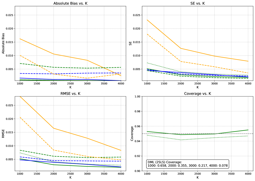
(b) $n=100,a_{\text{new}}=2$, $b_{\text{new}}=3.5$

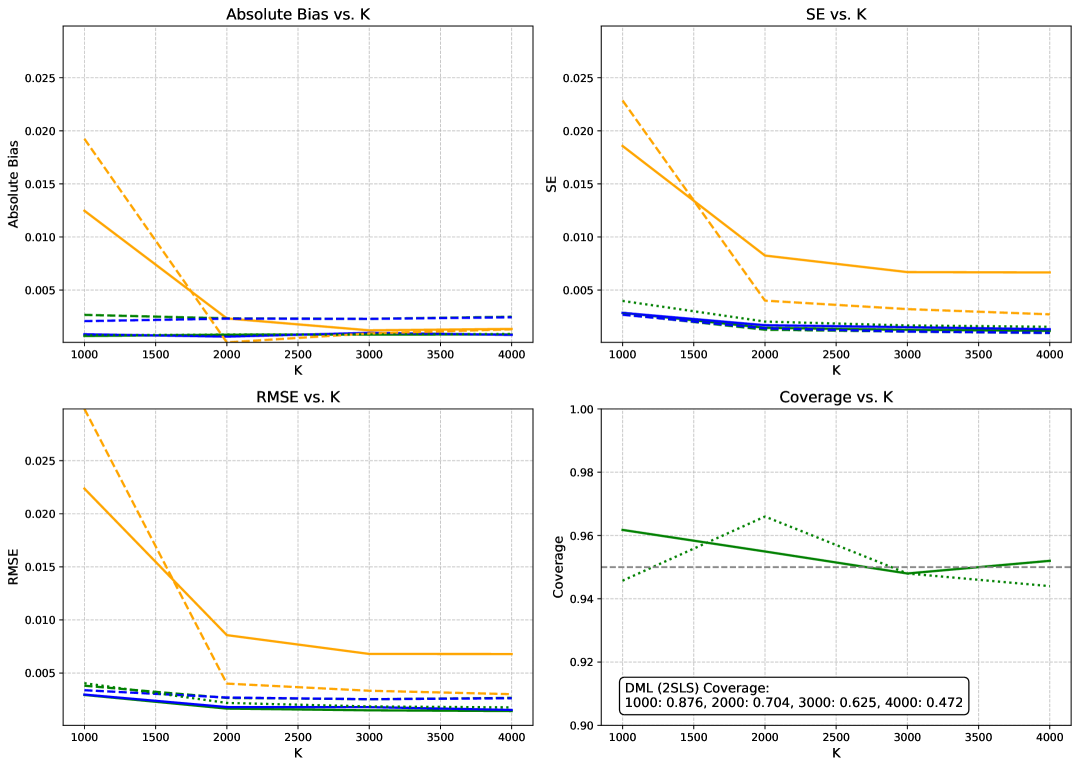
(c) $n=300,a_{\text{new}}=2$, $b_{\text{new}}=3.5$

Figure 1: Monte Carlo evaluation of estimation performance for the proposed cross-fold JIVE-based DML estimators, compared to single-fold JIVE DML, adversarial NPIV DML (2SLS), and plug-in and IPW estimators with and without cross-fold splitting. The plots show absolute bias, standard error (SE), root mean squared error (RMSE), and 95% confidence interval coverage for various $K$ and $n$. DML (2SLS) coverage values for each $K$ are reported in the coverage plots.

7.2 Simulation Results

Figure 1 displays Monte Carlo estimates of the absolute bias, standard error (SE), root mean squared error (RMSE), and 95% confidence interval coverage for the cross-fold (JIVE) and single-fold (JIVE 1-fold) DML estimators, as well as the baseline adversarial NPIV estimator (2SLS) that does not use cross-fold splitting. The figure also includes results for the plug-in and IPW estimators with and without cross-fold splitting (JIVE vs. 2SLS). Monte Carlo estimates are plotted for increasing numbers of instruments $K=1000,2000,3000,4000,5000$ and group-specific sample sizes $n=30$, $100$, and $300$.

The cross-fold JIVE-based DML estimator consistently achieves lower bias and RMSE compared to the single-fold JIVE DML and adversarial NPIV (2SLS) estimators, particularly when the number of instruments $K$ is large. Incorporating cross-fold splitting in the plug-in and IPW estimators also improves performance over their non-cross-fold counterparts, demonstrating the advantage of using JIVE. The coverage of the 95% confidence intervals for the DML (2SLS) estimator deteriorates rapidly as $K$ increases, especially for smaller sample sizes ($n=30$), where coverage rates drop to zero for $K=4000$ and fall below 10% for $K\geq 2000$. In contrast, the cross-fold JIVE-based estimators maintain reliable coverage across all settings, highlighting the importance of cross-fold splitting in improving both estimation accuracy and uncertainty quantification. We find that even with sample sizes as small as $n=30$, the cross-fold DML estimator achieves nominal coverage comparable to its single-fold counterpart and better estimation performance in terms of bias, standard error, and RMSE. This suggests that the potential lack of normality of the cross-fold DML estimator when $n_{k}\not\rightarrow\infty$ is not a significant issue in this experiment.

7.3 Asymptotic identification for linear regression

In this experiment, we consider inference on the structural coefficients in the NPIV problem within a high-dimensional linear model. Suppose $X\in\mathbb{R}^{d}$ is a feature vector with $d=200$, and the structural function satisfies $h_{F}^{\star}(x)=\langle X,\theta^{\star}\rangle_{\mathbb{R}^{d}}$, where $j^{\alpha}\theta^{\star}_{j}\in\{-1,1\}$ for $j\in[d]$ and an approximate sparsity parameter $\alpha>0$. The structural model is:

$$Y_{ki}=\langle X_{ki},\theta^{\star}\rangle_{\mathbb{R}^{d}}+\varepsilon_{ki}^{Y},\quad X_{ki}=\tilde{\Pi}_{k}+\varepsilon_{ki}^{X},$$

where $\tilde{\Pi}_{k}=(\tilde{\Pi}_{k,j})_{j\in\mathbb{N}}^{T}$ with $\tilde{\Pi}_{k,j}=j^{-\alpha}A_{k,j},$ and $A_{k,j}\overset{\text{iid}}{\sim}N(0,1).$ This model assumes the instrument $Z$ primarily influences $X$ through its leading components. Given an effective sparsity factor $1\leq s\leq d$, we choose the sparsity parameter $\alpha_{s}$ such that the vector $b_{\alpha}:=(j^{-\alpha})_{j=1}^{d}$ satisfies $s=\frac{\|b_{\alpha}\|_{\ell_{1}}^{2}}{\|b_{\alpha}\|_{\ell_{2}}^{2}},$ ensuring that $\theta^{\star}$ is well-approximated in $\ell^{2}$ by its first $s$ components. Our target of inference is $\psi(h_{F}^{\star})=\frac{1}{n}\sum_{i=1}^{n}h_{F}^{\star}(X_{K+1,i})$, where the new treatment $X_{K+1,i}$ is drawn as described by above.

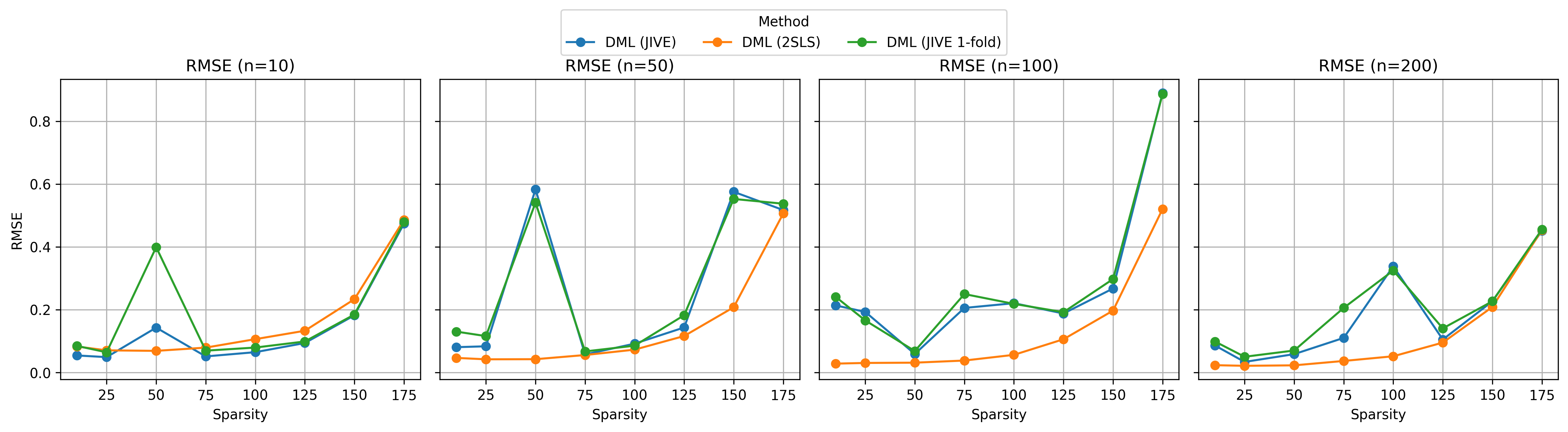
(a) RMSE Plot (2SLS)

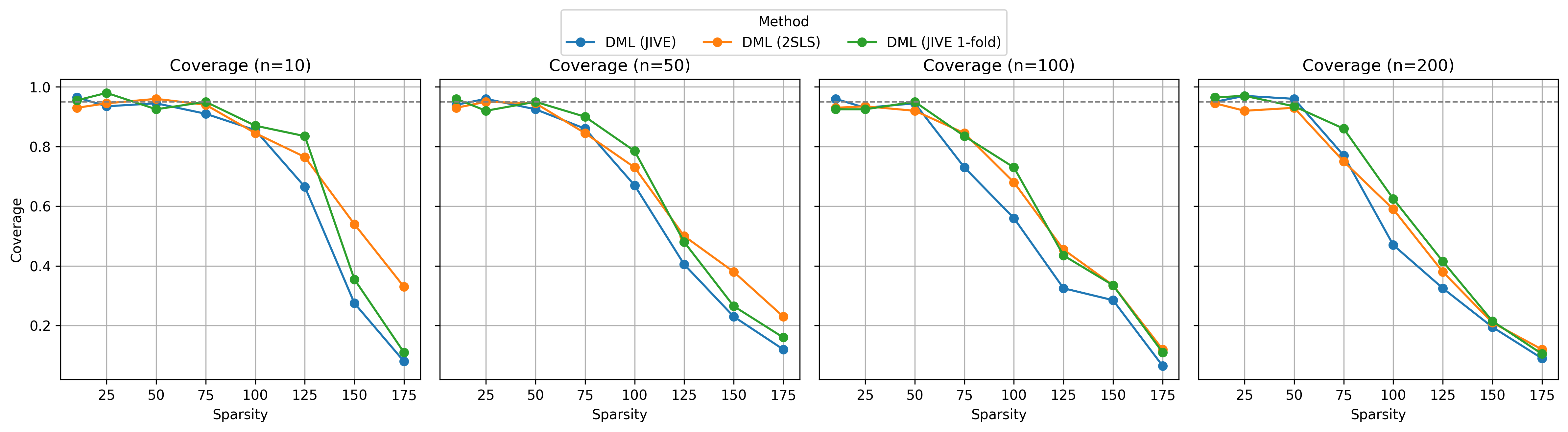
(b) Coverage Plot (2SLS)

Figure 2: Comparison of RMSE and Coverage Plots using 2SLS

In our experiments, we consider effective sparsity factors ranging from $10$ to $175$ with total dimension $d=200$ and the number of instruments $K=100$. Since $K<d$, strong identification does not hold in finite samples, and the functional $\psi(h_{F}^{\star})$ is only approximately identified, with the degree of approximation error determined by the approximate sparsity of $\theta^{\star}$. For various sparsity factors $s$ and sample sizes $n$, Figure 2 shows the root mean squared error (RMSE) and 95% confidence interval coverage for the cross-fold and single-fold DML estimators, as well as the baseline adversarial NPIV estimator that does not use cross-fold splitting. For sparsity factors between $10$ and $75$, all methods achieve nominal coverage, suggesting that asymptotic identification holds in this regime. As the sparsity factor increases, estimation error and coverage of all methods gradually deteriorate, consistent with the bias bound in Theorem 9, with coverage tending to zero as the solution becomes nonsparse due to failure of asymptotic identification. In this experiment, the number of instruments $K=100$ is of similar order to the sample size $n\in\{10,50,100,200\}$, resulting in similar performance across methods. We observe that cross-fold splitting decreases RMSE for $n=10$, while for larger sample sizes, RMSE and estimator stability is improved by not using cross-fold splitting. We note that cross-validation based on the JIVE empirical risks proposed in Section 5 can be used to adaptively select between nuisance estimators with and without cross-fold splitting.

Appendix A Additional experimental results

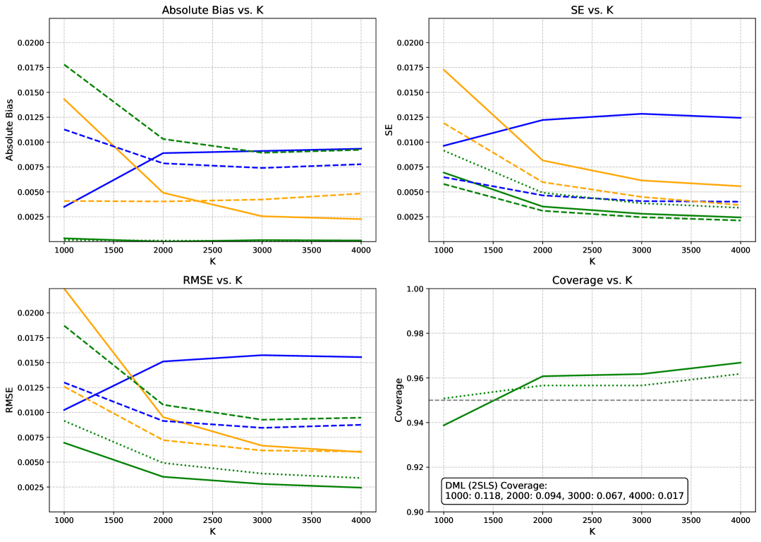
(a) $a_{\text{new}}=2$, $b_{\text{new}}=2.5$

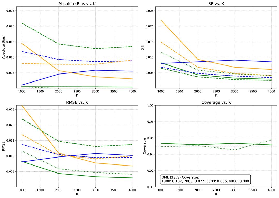
(b) $a_{\text{new}}=2$, $b_{\text{new}}=3$

(c) $a_{\text{new}}=2$, $b_{\text{new}}=3.5$

Figure 3: Comparison of Performance Metrics for Different Values of Overlap between treatment distribution in new experiment and marginal distribution of historical experiments.

Appendix B Additional details on examples

Denseness of $\mathcal{H}_{K}$ in Example 4.

Let $\mathcal{E}=\{e^{\theta x}:\theta\in(0,\varepsilon)\}.$ Suppose that $g$ is a function for which the Laplace transform

$$L_{g}(\theta)=\int g(x)e^{\theta x}\,dx$$

is analytic on $(0,\varepsilon)$ and satisfies

$$L_{g}(\theta)=0\quad\text{for all }\theta\in(0,\varepsilon).$$

Then by the identity theorem for analytic functions, it follows that $L_{g}(\theta)=0$ on the entire domain of analyticity, including $(0,\varepsilon)$. Under standard conditions ensuring the uniqueness of the Laplace transform (such as appropriate integrability and growth conditions on $g$), this implies that $g(x)=0$ almost everywhere. In other words, if the Laplace transform of $g$ vanishes on an interval, then $g$ itself must be the zero function (almost everywhere). Thus, the only function orthogonal to the linear span of $\mathcal{E}$ is the zero function, and by a standard Hilbert space argument, the span of $\mathcal{E}$ is dense in the space of functions whose Laplace transform exists on $(0,\varepsilon)$.

Now, consider the example where

$$g(x)=\frac{p^{\star}(x)}{p(x)},$$

with $p(x)>0$ and assume that the Laplace transform of $g$ exists on $(0,\varepsilon)$. Then, for every $\delta>0$, there exist $K$ large enough and coefficients $b_{k}$ and parameters $\theta_{k}\in(0,\varepsilon)$ such that

$$\Bigl{\|}g(x)-\sum_{k=1}^{K}b_{k}e^{\theta_{k}x}\Bigr{\|}<\delta.$$

Multiplying by $p(x)$, we obtain

$$\Bigl{\|}p^{\star}(x)-\sum_{k=1}^{K}b_{k}\,p(x)e^{\theta_{k}x}\Bigr{\|}<\delta\,\|p\|,$$

which shows that

$$p^{\star}(x)=p(x)g(x)=\sum_{k=1}^{\infty}b_{k}\,p(x)e^{\theta_{k}x},$$

with the approximation error vanishing as $K\to\infty$.

Now let $\{\theta_{k}\}_{k\geq 1}$ be an arbitrary sequence that is dense in $(0,\varepsilon)$. By the earlier density result, any function $f\in\mathcal{H}$ (in particular, any function whose Laplace transform exists on $(0,\varepsilon)$) can be approximated arbitrarily well by finite linear combinations of the form

$$f_{N}(x)=\sum_{j=1}^{N}c_{j}e^{\theta^{(j)}x},\quad\theta^{(j)}\in(0,\varepsilon).$$

Given $\delta>0$, choose such an approximation $f_{N}$ satisfying

$$\|f-f_{N}\|<\frac{\delta}{2}.$$

Since $\{\theta_{k}\}$ is dense in $(0,\varepsilon)$, for each $\theta^{(j)}$ there exists some $\theta_{k_{j}}$ with

$$|\theta^{(j)}-\theta_{k_{j}}|<\eta,$$

where $\eta>0$ is small enough that

$$\|e^{\theta^{(j)}x}-e^{\theta_{k_{j}}x}\|<\frac{\delta}{2N\max_{1\leq j\leq N}|c_{j}|}.$$

Define the alternative approximation

$$g_{N}(x)=\sum_{j=1}^{N}c_{j}e^{\theta_{k_{j}}x}.$$

Then, by the triangle inequality,

$$\|f-g_{N}\|\leq\|f-f_{N}\|+\|f_{N}-g_{N}\|<\frac{\delta}{2}+\sum_{j=1}^{N}|c_{j}|\|e^{\theta^{(j)}x}-e^{\theta_{k_{j}}x}\|<\frac{\delta}{2}+\frac{\delta}{2}=\delta.$$

Since $\delta>0$ was arbitrary, it follows that the linear span of $\{e^{\theta_{k}x}:k\geq 1\}$ is dense in $\mathcal{H}$. Consequently, any function in $\mathcal{H}$ (and thus any function whose Laplace transform exists on $(0,\varepsilon)$) can be approximated arbitrarily well by a linear combination of $e^{\theta_{k}x}$, with $\theta_{k}\in(0,\varepsilon)$.

∎

Appendix C Proofs of asymptotic identification

Proof of Theorem 2.

By properties of the pseudoinverse, it holds that $h^{\star}_{K}=\Pi_{K}h^{\star}_{F}$. By the Riesz representation theorem, we have

$$\Psi^{(K)}(P^{(K)})-\psi(h_{F}^{\star}) =\langle\alpha_{K},h^{\star}_{K}\rangle_{L^{2}_{K}(X)}-\langle\alpha_{K},h^{\star}_{F}\rangle_{L^{2}_{K}(X)}$$

$$=\langle\alpha_{K},h^{\star}_{K}-h^{\star}_{F}\rangle_{L^{2}_{K}(X)}$$

$$=\langle\alpha_{K},\Pi_{K}h^{\star}_{F}-h^{\star}_{F}\rangle_{L^{2}_{K}(X)}$$

$$=\langle\alpha_{K}-\Pi_{K}\alpha_{K},\Pi_{K}h^{\star}_{F}-h^{\star}_{F}\rangle_{L^{2}_{K}(X)},$$

where the final equality follows from the orthogonality condition of the projection, which ensures that

$$\langle\Pi_{K}\alpha_{K},\Pi_{K}h^{\star}_{F}-h^{\star}_{F}\rangle_{L^{2}_{K}(X)}=0.$$

∎

Appendix D Proofs for convergence rate of primal solution

Proof of Theorem 4.

The proof of Theorem 4 is analogous to that of Theorem 6. The rate without the source condition ($\nu=0$) was established in Theorem 1 of Bibaut et al. (2024). ∎

Appendix E Proofs for convergence rate of debiasing nuisance

E.1 Proof of bounds for oracle bias

Proof of Theorem 5.

We use the fact that the source condition $\Pi_{K}\alpha_{K}\in\mathcal{R}((\mathcal{T}_{K}^{*}\mathcal{T}_{K})^{1+\nu})$ for some $\nu>0$ implies that $\beta_{K}\in\mathcal{R}((\mathcal{T}_{K}^{*}\mathcal{T}_{K})^{\nu})$. To see this, let $(\mathcal{T}_{K}^{*}\mathcal{T}_{K})^{\dagger}$ denote the inverse of the restriction of $\mathcal{T}_{K}^{*}\mathcal{T}_{K}$ to $\mathcal{H}_{K}(X)$. Then, noting that $\Pi_{K}\alpha_{K}\in\mathcal{H}_{K}(X)$, we know that $\beta_{K}=(\mathcal{T}_{K}^{*}\mathcal{T}_{K})^{+}\Pi_{K}\alpha_{K}=(\mathcal{T}_{K}^{*}\mathcal{T}_{K})^{\dagger}(\mathcal{T}_{K}^{*}\mathcal{T}_{K})^{1+\nu}\omega_{K}$ , where $\Pi_{K}\alpha_{K}=(\mathcal{T}_{K}^{*}\mathcal{T}_{K})^{\nu}\omega_{K}$. Thus, $\beta_{K}=(\mathcal{T}_{K}^{*}\mathcal{T}_{K})^{\nu}\omega_{K}$, as desired.

Strong norm rate.

For the strong norm, we will establish the following two bounds:

$$\|(\mathcal{T}_{K}^{*}\mathcal{T}_{K}+\lambda I)^{-1}\Pi_{K}\alpha_{K}-\beta_{K}\| \leq O(\lambda^{\nu})\,\|w_{K}\|$$ (6)

$$\|(\mathcal{T}_{K}^{*}\mathcal{T}_{K}+\lambda I)^{-1}(\alpha_{K}-\Pi_{K}\alpha_{K})\| \leq O(\lambda^{-1})\,\|\alpha_{K}-\Pi_{K}\alpha_{K}\|$$ (7)

Taking the above bounds as given for the moment, observe that:

$$\beta_{K}(\lambda)-\beta_{K}\;=\;\Bigl{[}(\mathcal{T}_{K}^{*}\mathcal{T}_{K}+\lambda I)^{-1}\,\Pi_{K}\alpha_{K}-\beta_{K}\Bigr{]}\;+\;(\mathcal{T}_{K}^{*}\mathcal{T}_{K}+\lambda I)^{-1}\,(\alpha_{K}-\Pi_{K}\alpha_{K}).$$

Thus,

$$\|\beta_{K}(\lambda)-\beta_{K}\|\;=\;O(\lambda^{\nu})\,\|w_{K}\|\;+\;O(\lambda^{-1})\,\|\alpha_{K}-\Pi_{K}\alpha_{K}\|.$$

Optimizing the choice of $\lambda$ (the bias-variance trade-off) yields $\lambda\sim\|\alpha_{K}-\Pi_{K}\alpha_{K}\|^{\frac{1}{1+\nu}}$ and

$$\|\beta_{K}(\lambda)-\beta_{K}\|\leq\|\alpha_{K}-\Pi_{K}\alpha_{K}\|^{\frac{\nu}{1+\nu}}$$

Weak norm rate.

For the weak norm, observe that:

$$\mathcal{T}_{K}\beta_{K}(\lambda)-\mathcal{T}_{K}\beta_{K}\;=\;\Bigl{[}\mathcal{T}_{K}(\mathcal{T}_{K}^{*}\mathcal{T}_{K}+\lambda I)^{-1}\,\Pi_{K}\alpha_{K}-\mathcal{T}_{K}\beta_{K}\Bigr{]}\;+\;\mathcal{T}_{K}(\mathcal{T}_{K}^{*}\mathcal{T}_{K}+\lambda I)^{-1}\,(\alpha_{K}-\Pi_{K}\alpha_{K}).$$

We will establish the following two bounds:

$$\|\mathcal{T}_{K}(\mathcal{T}_{K}^{*}\mathcal{T}_{K}+\lambda I)^{-1}\Pi_{K}\alpha_{K}-\beta_{K}\| \leq O(\lambda^{\nu+\frac{1}{2}})\,\|w_{K}\|$$ (8)

$$\|\mathcal{T}_{K}(\mathcal{T}_{K}^{*}\mathcal{T}_{K}+\lambda I)^{-1}(\alpha_{K}-\Pi_{K}\alpha_{K})\| \leq O(\lambda^{-1/2})\,\|\alpha_{K}-\Pi_{K}\alpha_{K}\|.$$ (9)

Thus,

$$\|\mathcal{T}_{K}\beta_{K}(\lambda)-\mathcal{T}_{K}\beta_{K}\|\;=\;O(\lambda^{\nu+\frac{1}{2}})\,\|w_{K}\|\;+\;O(\lambda^{-1/2})\,\|\alpha_{K}-\Pi_{K}\alpha_{K}\|.$$

Optimizing the choice of $\lambda$ (the bias-variance trade-off) yields $\lambda\sim\left(\|\alpha_{K}-\Pi_{K}\alpha_{K}\|\right)^{\frac{1}{\nu+1}}$ and

$$\|\mathcal{T}_{K}\beta_{K}(\lambda)-\mathcal{T}_{K}\beta_{K}\|\;\leq\;\|\alpha_{K}-\Pi_{K}\alpha_{K}\|^{\frac{\nu+\frac{1}{2}}{\nu+1}}.$$

Proof of regularization error bounds.

These bounds follow from the proof of Lemma 3 in Bennett et al. (2023). Since $\Pi_{K}\alpha_{K}\in\mathcal{R}(\mathcal{T}_{K}^{*})$ and $\mathcal{T}_{K}^{*}\mathcal{T}_{K}$ is invertible on $\mathcal{R}(\mathcal{T}_{K}^{*})$, note $\Pi_{K}\alpha_{K}\;=\;\mathcal{T}_{K}^{*}\mathcal{T}_{K}\,\beta_{K}$ implies that

$$(\mathcal{T}_{K}^{*}\mathcal{T}_{K}+\lambda I)^{-1}\,\Pi_{K}\alpha_{K}\;-\;\beta_{K}\;=\;(\mathcal{T}_{K}^{*}\mathcal{T}_{K}+\lambda I)^{-1}\,\mathcal{T}_{K}^{*}\mathcal{T}_{K}\,\beta_{K}\;-\;\beta_{K}.$$

A standard argument in regularization theory (using functional calculus or the resolvent identity) shows that if $\beta_{K}\in\mathcal{R}((\mathcal{T}_{K}^{*}\mathcal{T}_{K})^{\nu})$, then the norm of the latter term in the previous display satisfies

$$\Bigl{\|}\Bigl{[}I\;-\;(\mathcal{T}_{K}^{*}\mathcal{T}_{K}+\lambda I)^{-1}\mathcal{T}_{K}^{*}\mathcal{T}_{K}\Bigr{]}\beta_{K}\Bigr{\|}=O(\lambda^{\nu})\,\|w_{K}\|.$$

For details, we refer to the proof of Lemma 3 in Bennett et al. (2023). Hence, $\|(\mathcal{T}_{K}^{*}\mathcal{T}_{K}+\lambda I)^{-1}\Pi_{K}\alpha_{K}\;-\;\beta_{K}\|\;=\;O(\lambda^{\nu})\,\|w_{K}\|.$ The proof of Lemma 3 in Bennett et al. (2023) also establishes the weak norm bound $\|\mathcal{T}_{K}(\mathcal{T}_{K}^{*}\mathcal{T}_{K}+\lambda I)^{-1}\Pi_{K}\alpha_{K}\;-\;\beta_{K}\|\;=\;O(\lambda^{\frac{1}{2}+\nu})\,\|w_{K}\|.$

Proof of approximation error bounds.

For the strong norm bound. Consider $(A+\lambda I)^{-1}\bigl{(}\alpha_{K}-\Pi_{K}\alpha_{K}\bigr{)},$ where $A=\mathcal{T}_{K}^{*}\mathcal{T}_{K}$. Then

$$\|(A+\lambda I)^{-1}(\alpha_{K}-\Pi_{K}\alpha_{K})\| \leq\|(A+\lambda I)^{-1}\|_{\text{op}}\|\alpha_{K}-\Pi_{K}\alpha_{K}\|$$

$$\leq\frac{1}{\lambda}\|\alpha_{K}-\Pi_{K}\alpha_{K}\|,$$

where we use the standard bound $\|(A+\lambda I)^{-1}\|_{\text{op}}=\sup_{\sigma\in\text{spec}(A)}\frac{1}{\sigma+\lambda}\lesssim\lambda^{-1}.$

For the weak norm bound, similarly, we can show that

$$\|\mathcal{T}_{K}(\mathcal{T}_{K}^{*}\mathcal{T}_{K}+\lambda I)^{-1}(\alpha_{K}-\Pi_{K}\alpha_{K})\| \leq\|\mathcal{T}_{K}(\mathcal{T}_{K}^{*}\mathcal{T}_{K}+\lambda I)^{-1}\|_{\text{op}}\|\alpha_{K}-\Pi_{K}\alpha_{K}\|$$

$$\leq\sup_{\sigma\in\text{spec}(\mathcal{T}_{K}^{*}\mathcal{T}_{K})}\frac{\sigma}{\sigma^{2}+\lambda}\|\alpha_{K}-\Pi_{K}\alpha_{K}\|$$

$$\leq O\left(\lambda^{-1/2}\right)\|\alpha_{K}-\Pi_{K}\alpha_{K}\|.$$

∎

E.2 Technical lemmas based on local maximal inequalities

Lemma 1.

Suppose that $\mathcal{F}$ is a star-shaped and uniformly bounded function class. Define $\delta_{n}:=\max_{k\in[K]}\delta_{n_{k}}$, where each $\delta_{n_{k}}$ satisfies the critical inequality $E_{K}[\widehat{\mathcal{R}}_{n_{k}}(\mathcal{F},\delta)]\leq\delta^{2}\sqrt{n_{k}}$ and the growth condition $n_{k}^{-1/2}\sqrt{\log\log\delta_{n_{k}}}=o(\delta_{n_{k}})$. Then, with probability at least $1-e^{\log K-\min_{k\in[K]}\{\delta_{n,k}^{2}n_{k}\}}$, the following holds uniformly for all $f\in\mathcal{F}$ and $k\in[K]$:

$$\left|\widehat{\mathcal{T}}_{K,0}(f)(k)-\mathcal{T}_{K}(f)(k)\right|\lesssim\delta_{n}\|f\|_{k}+\delta_{n}^{2}.$$

Proof.

By Lemma 9 of Bibaut et al. (2024), we have, for any $u_{k}\geq 0$, with probability at least $1-e^{-u_{k}^{2}}$, the following holds uniformly for all $f\in\mathcal{F}$:

$$\widehat{\mathcal{T}}_{K,0}(f)(k)-\mathcal{T}_{K}(f)(k)\lesssim\delta_{n_{k}}\|f\|_{k}+\delta_{n_{k}}^{2}+\frac{u_{k}\|f\|_{k}}{\sqrt{n_{k}}}+\frac{u_{k}^{2}}{\sqrt{n_{k}}}.$$

Setting $u_{k}=\delta_{n_{k}}\sqrt{n_{k}}$ and applying a union bound, with probability at least $1-\sum_{k=1}^{K}e^{-\delta_{n,k}^{2}n_{k}}\geq 1-e^{\log K-\min_{k\in[K]}\{\delta_{n,k}^{2}n_{k}\}}$, we have $\widehat{\mathcal{T}}_{K,0}(f)(k)-\mathcal{T}_{K}(f)(k)\lesssim\delta_{n_{k}}\|f\|_{k}+\delta_{n_{k}}^{2}.$

∎

Lemma 2.

Suppose that $\mathcal{F}$ is a uniformly bounded function class. Define the function class $\mathcal{G}:=\{g_{f}:f\in\mathcal{F}\}$, where $g_{f}:=\mathcal{T}_{K}(f)\{f-\mathcal{T}_{K}(f)\}$. Let $\delta_{N}$ satisfy the critical inequality $E_{K}[\widehat{\mathcal{R}}_{N}(\text{star}(\mathcal{G}),\delta)]\leq\sqrt{N}\delta^{2}$ and $N^{-1/2}\sqrt{\log\log\delta_{N}}=o(\delta_{N}).$ Then, with probability at least $1-e^{-N\delta_{N}^{2}}$, we have

$$\langle\mathcal{T}_{K}(f),[\widehat{\mathcal{T}}_{K,v}-\mathcal{T}_{K}](f)\rangle_{L^{2}_{K}(Z)}\lesssim\delta_{N}\|\mathcal{T}_{K}(f)\|_{L^{2}_{K}(Z)}+\delta_{N}^{2}.$$

Proof.

For each $v\in\{0,1\}$, we can write

$$\langle\mathcal{T}_{K}(f),\widehat{\mathcal{T}}_{K,v}(f)-\mathcal{T}_{K}(f)\rangle_{L^{2}_{K}(Z)}=\frac{1}{N}\sum_{k=1}^{K}\sum_{i=1}^{n_{k}}1(V_{ki}=v)\mathcal{T}_{K}(f)(k)\left\{f(X_{ki})-\mathcal{T}_{K}(f)(k)\right\},$$

where the right-hand side is an empirical mean of approximately $N/2$ random variables with mean zero. We will use this fact to show that this term uniformly concentrates around zero.

Define the function class $\mathcal{G}:=\{g_{f}:f\in\mathcal{F}\}$, where $g_{f}:=\mathcal{T}_{K}(f)\{f-\mathcal{T}_{K}(f)\}$. Applying the local maximal inequality stated in Lemma 9 of Bibaut et al. (2024), we find that for any $u\geq 0$, with probability at least $1-e^{-u^{2}}$, the following holds for any $f\in\mathcal{F}$:

$$\langle\mathcal{T}_{K}(f),[\widehat{\mathcal{T}}_{K,v}-\mathcal{T}_{K}](f)\rangle_{L^{2}_{K}(Z)}\lesssim\delta_{N}\|g_{f}\|_{L^{2}_{K}}+\delta_{N}^{2}+\frac{u\|g_{f}\|_{L^{2}_{K}}}{\sqrt{N}}+\frac{u^{2}}{N}.$$

where $\delta_{N}$ satisfies the critical inequality $E_{K}[\widehat{\mathcal{R}}_{N}(\mathcal{G},\delta)]\leq\sqrt{N}\delta^{2}$ and $N^{-1/2}\sqrt{\log\log\delta_{N}}=o(\delta_{N}).$ Since $\mathcal{F}$ is uniformly bounded, we can further bound $\|g_{f}\|_{L^{2}_{K}}$ loosely as

$$\|g_{f}\|_{L^{2}_{K}} =\sqrt{\sum_{k=1}^{K}\frac{n_{k}}{N}\{\mathcal{T}_{K}(f)(k)\}^{2}E_{K}\left[\{f(X_{k})-\mathcal{T}_{K}(f)(k)\}^{2}\right]}$$

$$\lesssim\min\left\{\|\mathcal{T}_{K}(f)\|_{L^{2}_{K}(Z)},\,\|f\|_{L^{2}_{K}}\right\}.$$

Thus, for any $u\geq 0$, with probability at least $1-e^{-u^{2}}$, the following holds for any $f\in\mathcal{F}$:

$$\langle\mathcal{T}_{K}(f),[\widehat{\mathcal{T}}_{K,v}-\mathcal{T}_{K}](f)\rangle_{L^{2}_{K}(Z)}\lesssim\delta_{N}\|\mathcal{T}_{K}(f)\|_{L^{2}_{K}(Z)}+\delta_{N}^{2}+\frac{u}{\sqrt{N}}\|\mathcal{T}_{K}(f)\|_{L^{2}_{K}(Z)}+\frac{u^{2}}{N}.$$

Setting $u=\delta_{n}\sqrt{N}$, with probability at least $1-e^{-N\delta_{N}^{2}}$, we have

$$\langle\mathcal{T}_{K}(f),[\widehat{\mathcal{T}}_{K,v}-\mathcal{T}_{K}](f)\rangle_{L^{2}_{K}(Z)}\lesssim\delta_{N}\|\mathcal{T}_{K}(f)\|_{L^{2}_{K}(Z)}+\delta_{N}^{2}.$$

∎

Lemma 3.

Suppose that $\mathcal{F}$ be a uniformly bounded function class, and let $f_{0}\in\mathcal{F}$. Define the function class $\mathcal{G}:=\{g_{f}:f\in\mathcal{F}\}$, where $g_{f}:=f\cdot\mathcal{T}_{K}(f-f_{0})$. Let $\delta_{N}$ satisfy the critical inequality $E_{K}[\widehat{\mathcal{R}}_{N}(\text{star}(\mathcal{G}),\delta)]\leq\sqrt{N}\delta^{2}$ and $N^{-1/2}\sqrt{\log\log\delta_{N}}=o(\delta_{N}).$ Then, with probability at least $1-e^{-N\delta_{N}^{2}}$, we have

$$\langle\widehat{\mathcal{T}}_{K,v}(f),\mathcal{T}_{K}(f-f_{0})\rangle_{L^{2}_{K}(Z)}-\langle\mathcal{T}_{K}(f),\mathcal{T}_{K}(f-f_{0})\rangle_{L^{2}_{K}(Z)}\lesssim\delta_{N}\|\mathcal{T}_{K}(f-f_{0})\|_{L^{2}_{K}(Z)}+\delta_{N}^{2}.$$

Proof.

The proof of this lemma is nearly identical to the proof of Lemma 2. By independence of the folds, we can express $\langle\widehat{\mathcal{T}}_{K,v}(f),\mathcal{T}_{K}(f-f_{0})\rangle_{L^{2}_{K}(Z)}$ as the empirical mean of mean zero-random variables:

$$\frac{1}{N}\sum_{k=1}^{K}\sum_{i=1}^{n_{k}}1(V_{ki}=v)\{f(X_{ki})-\mathcal{T}_{K}(f)\}\mathcal{T}_{K}(f-f_{0})(k).$$

Applying Lemma 9 of Bibaut et al. (2024), with probability at least $1-e^{-N\delta_{N}^{2}}$, we have

$$\langle\widehat{\mathcal{T}}_{K,v}(f-\mathcal{T}_{K}f),\mathcal{T}_{K}(f-f_{0})\rangle_{L^{2}_{K}(Z)}\lesssim\delta_{N}\|\mathcal{T}_{K}(f-f_{0})\|_{L^{2}_{K}(Z)}+\delta_{N}^{2}.$$

∎

Lemma 4.

Suppose that $\mathcal{F}$ is a uniformly bounded function class, where $\|f-\mathcal{T}_{K}(f)\|_{\infty}\lesssim\|f-\mathcal{T}_{K}(f)\|_{L^{2}_{K}}^{1-\kappa}$ for each $f\in\mathcal{F}$. This condition always holds with $\kappa=1$. Define the function class $\widehat{\mathcal{G}}:=\{\widehat{g}_{f}:f\in\mathcal{F}\}$ as the set of all elements of the form $\widehat{g}_{f}:=[\widehat{\mathcal{T}}_{K,0}-\mathcal{T}_{K}](f)\{f-\mathcal{T}_{K}(f)\}$. Let $\delta_{N}$ satisfy the critical inequality $E_{K}[\widehat{\mathcal{R}}_{N}(\text{star}(\widehat{\mathcal{G}}),\delta)\mid\mathcal{D}_{n,0}]\leq\sqrt{N}\delta^{2}$ and $N^{-1/2}\sqrt{\log\log\delta_{N}}=o(\delta_{N}).$ Let $\delta_{n}^{2}:=\max_{k\in[K]}\delta_{n_{k}}^{2}$, where each $\delta_{n_{k}}$ satisfies the critical inequality $E_{K}[\widehat{\mathcal{R}}_{n_{k}}(\text{star}(\mathcal{F}),\delta)]\leq\delta^{2}\sqrt{n_{k}}$ and $n_{k}^{-1/2}\sqrt{\log\log\delta_{n_{k}}}=o(\delta_{n_{k}})$ Then, with probability at least $1-e^{\log K-N\delta_{N}^{2}}-e^{\log K-\min_{k\in[K]}\{\delta_{n,k}^{2}n_{k}\}}$, the following holds uniformly for any $f\in\mathcal{F}$:

$$\langle\widehat{\mathcal{T}}_{K,0}(f)-\mathcal{T}_{K}(f),\widehat{\mathcal{T}}_{K,1}(f)-\mathcal{T}_{K}(f)\rangle_{L^{2}_{K}(Z)} \lesssim\delta_{N}\delta_{n}\|f-\mathcal{T}_{K}(f)\|_{L^{2}_{K}}^{2-\kappa}$$

$$\quad+\delta_{N}\delta_{n}^{2}\|f-\mathcal{T}_{K}(f)\|_{L^{2}_{K}}+\delta_{N}^{2}.$$

Lemma 5.

Suppose that $\mathcal{F}$ is a uniformly bounded function class, and let $f_{0}\in\mathcal{F}$. Define the function class $\widehat{\mathcal{G}}:=\{\widehat{g}_{f}:f\in\mathcal{F}\}$ as the set of all elements of the form $\widehat{g}_{f}:=\widehat{\mathcal{T}}_{K,v}(f)\{f-f_{0}-\mathcal{T}_{K}(f-f_{0})\}$. Let $\delta_{N}$ satisfy the critical inequality $E_{K}[\widehat{\mathcal{R}}_{N}(\text{star}(\widehat{\mathcal{G}}),\delta)\mid\mathcal{D}_{n,v}]\leq\sqrt{N}\delta^{2}$ and $N^{-1/2}\sqrt{\log\log\delta_{N}}=o(\delta_{N}).$ Let $\delta_{n}^{2}:=\max_{k\in[K]}\delta_{n_{k}}^{2}$, where each $\delta_{n_{k}}$ satisfies the critical inequality $E_{K}[\widehat{\mathcal{R}}_{n_{k}}(\text{star}(\mathcal{F}),\delta)]\leq\delta^{2}\sqrt{n_{k}}$ and $n_{k}^{-1/2}\sqrt{\log\log\delta_{n_{k}}}=o(\delta_{n_{k}})$ Then, with probability at least $1-e^{\log K-N\delta_{N}^{2}}-e^{\log K-\min_{k\in[K]}\{\delta_{n,k}^{2}n_{k}\}}$, the following holds uniformly for any $f\in\mathcal{F}$:

$$\langle\widehat{\mathcal{T}}_{K,0}(f),\widehat{\mathcal{T}}_{K,1}(f-f_{0})-\mathcal{T}_{K}(f-f_{0})\rangle_{L^{2}_{K}(Z)} \lesssim\delta_{N}\delta_{n}\|f-f_{0}\|_{L^{2}_{K}}$$

$$\quad+\delta_{N}\delta_{n}^{2}+\delta_{N}^{2}.$$

Proof of Lemma 4.

We can express $\langle\widehat{\mathcal{T}}_{K,0}(f)-\mathcal{T}_{K}(f),\widehat{\mathcal{T}}_{K,1}(f)-\mathcal{T}_{K}(f)\rangle_{L^{2}_{K}(Z)}$ as the empirical mean:

$$\frac{1}{N}\sum_{k=1}^{K}\sum_{i=1}^{n_{k}}1(V_{ki}=1)\left\{\widehat{\mathcal{T}}_{K,0}(f)-\mathcal{T}_{K}(f)\right\}\left\{f(X_{ki})-\mathcal{T}_{K}(f)(k)\right\}.$$

Moreover, from the independence of the data folds, the right-hand side is mean zero conditional on the data fold $\mathcal{D}_{n,0}$:

$$\sum_{k=1}^{K}\frac{n_{k}}{N}E_{K}\Big{[}\big{\{}\widehat{\mathcal{T}}_{K,0}(f)(k) -\mathcal{T}_{K}(f)\big{\}}\big{\{}f(X_{k})-\mathcal{T}_{K}(f)(k)\big{\}}\mid\mathcal{D}_{n,0}\Big{]}$$

$$=\sum_{k=1}^{K}\frac{n_{k}}{N}\big{\{}\widehat{\mathcal{T}}_{K,0}(f)(k)-\mathcal{T}_{K}(f)(k)\big{\}}E_{K}\big{[}f(X_{k})-\mathcal{T}_{K}(f)(k)\big{]}=0.$$

Define the function class $\widehat{\mathcal{G}}:=\{\widehat{g}_{f}:f\in\mathcal{F}\}$ as the set of all elements of the form $\widehat{g}_{f}:=[\widehat{\mathcal{T}}_{K,0}-\mathcal{T}_{K}](f)\{f-\mathcal{T}_{K}(f)\}$. Note that $\big{\{}\widehat{\mathcal{T}}_{K,0}(f)-\mathcal{T}_{K}(f)\big{\}}\big{\{}f-\mathcal{T}_{K}(f)\big{\}}$ is an element of $\widehat{\mathcal{G}}$ with probability at least $1-e^{-\delta_{n}^{2}N/K}$. Thus, applying Lemma 9 of Bibaut et al. (2024), conditionally on the training fold $\mathcal{D}_{n,0}$, we find, with probability at least $1-e^{-N\delta_{N}^{2}}$, the following holds uniformly for any $f\in\mathcal{F}$:

$$\langle\widehat{\mathcal{T}}_{K,0}(f)-\mathcal{T}_{K}(f),\widehat{\mathcal{T}}_{K,1}(f)-\mathcal{T}_{K}(f)\rangle_{L^{2}_{K}(Z)}\lesssim\delta_{N}\|\widehat{g}_{f}\|_{L^{2}_{K}}+\delta_{N}^{2}.$$

where $\delta_{N}$ satisfies $E_{K}[\widehat{\mathcal{R}}_{N}(\widehat{\mathcal{G}},\delta)\mid\mathcal{D}_{n,0}]\leq\sqrt{N}\delta^{2}$ and $N^{-1/2}\sqrt{\log\log\delta_{N}}=o(\delta_{N}).$

Now, define $\delta_{n}^{2}:=\max_{k\in[K]}\delta_{n_{k}}^{2}$, where each $\delta_{n_{k}}$ satisfies the critical inequality $E_{K}[\widehat{\mathcal{R}}_{n_{k}}(\mathcal{F},\delta)]\leq\delta^{2}\sqrt{n_{k}}$ and $n_{k}^{-1/2}\sqrt{\log\log\delta_{n_{k}}}=o(\delta_{n_{k}})$. Then, by Lemma 1, there exists a constant $C\geq 0$ such that, with probability at least $1-e^{\log K-\min_{k\in[K]}\{\delta_{n,k}^{2}n_{k}\}}$, the following holds uniformly over all $f\in\mathcal{F}$:

$$\|\widehat{g}_{f}\|_{L^{2}_{K}}^{2} =\|[\widehat{\mathcal{T}}_{K,0}-\mathcal{T}_{K}](f)\{f-\mathcal{T}_{K}(f)\}\|_{L^{2}_{K}}^{2}$$

$$=\sum_{k=1}^{N}\frac{n_{k}}{N}\{[\widehat{\mathcal{T}}_{K,0}-\mathcal{T}_{K}](f)(k)\}^{2}\|f-\mathcal{T}_{K}(f)\|_{k}^{2}$$

$$\leq\sum_{k=1}^{N}\frac{n_{k}}{N}\left\{\delta_{n}\|f-\mathcal{T}_{K}(f)\|_{k}+\delta_{n}^{2}\right\}^{2}\|f-\mathcal{T}_{K}(f)\|_{k}^{2}$$

$$\lesssim\delta_{n}^{2}\left[\sum_{k=1}^{N}\frac{n_{k}}{N}\|f-\mathcal{T}_{K}(f)\|_{k}^{4}\right]+\delta_{n}^{4}\|f-\mathcal{T}_{K}(f)\|_{L^{2}_{K}}^{2}$$

$$\lesssim\delta_{n}^{2}\|f-\mathcal{T}_{K}(f)\|_{\infty}^{2}\|f-\mathcal{T}_{K}(f)\|_{L^{2}_{K}}^{2}+\delta_{n}^{4}\|f-\mathcal{T}_{K}(f)\|_{L^{2}_{K}}^{2}.$$

Thus, we have $\|\widehat{g}_{f}\|_{L^{2}_{K}}\lesssim\delta_{n}\|f-\mathcal{T}_{K}(f)\|_{L^{2}_{K}}^{2-\kappa}+\delta_{n}^{2}\|f-\mathcal{T}_{K}(f)\|_{L^{2}_{K}}$, since $\|f-\mathcal{T}_{K}(f)\|_{\infty}\lesssim\|f-\mathcal{T}_{K}(f)\|_{L^{2}_{K}}^{1-\kappa}$.

Putting it all together, we find, with probability at least $1-e^{\log K-N\delta_{N}^{2}}-e^{\log K-\min_{k\in[K]}\{\delta_{n,k}^{2}n_{k}\}}$, the following holds uniformly for any $f\in\mathcal{F}$:

$$\langle\widehat{\mathcal{T}}_{K,0}(f)-\mathcal{T}_{K}(f),\widehat{\mathcal{T}}_{K,1}(f)-\mathcal{T}_{K}(f)\rangle_{L^{2}_{K}(Z)} \lesssim\delta_{N}\delta_{n}\|f-\mathcal{T}_{K}(f)\|_{L^{2}_{K}}^{2-\kappa}$$

$$\quad+\delta_{N}\delta_{n}^{2}\|f-\mathcal{T}_{K}(f)\|_{L^{2}_{K}}+\delta_{N}^{2}.$$

∎

Proof of Lemma 5.

The proof of this lemma is nearly identical to the proof of Lemma 4. By independence of the folds, we can express $\langle\widehat{\mathcal{T}}_{K,0}(f),\widehat{\mathcal{T}}_{K,1}(f-f_{0})-\mathcal{T}_{K}(f-f_{0})\rangle_{L^{2}_{K}(Z)}$ as the empirical mean of mean zero-random variables:

$$\frac{1}{N}\sum_{k=1}^{K}\sum_{i=1}^{n_{k}}1(V_{ki}=0)f(X_{ki})\left\{\widehat{\mathcal{T}}_{K,1}(f-f_{0})(k)-\mathcal{T}_{K}(f-f_{0})(k)\right\}.$$

Applying Lemma 9 of Bibaut et al. (2024), conditionally on the training fold $\mathcal{D}_{n,1}$, we find, with probability at least $1-e^{-N\delta_{N}^{2}}$, the following holds uniformly for any $f\in\mathcal{F}$:

$$\langle\widehat{\mathcal{T}}_{K,0}(f),\widehat{\mathcal{T}}_{K,1}(f-f_{0})-\mathcal{T}_{K}(f-f_{0})\rangle_{L^{2}_{K}(Z)}\lesssim\delta_{N}\|f\{\widehat{\mathcal{T}}_{K,1}(f-f_{0})-\mathcal{T}_{K}(f-f_{0})\}\|_{L^{2}_{K}}+\delta_{N}^{2}.$$

To complete the proof, we will now show that $\|f\{\widehat{\mathcal{T}}_{K,1}(f-f_{0})-\mathcal{T}_{K}(f-f_{0})\}\|_{L^{2}_{K}}^{2}\lesssim\delta_{n}\|f-f_{0}\|_{L^{2}_{K}(X)}+\delta_{n}^{2}$ with high probability. By Lemma 1, there exists a constant $C\geq 0$ such that, with probability at least $1-e^{\log K-\min_{k\in[K]}\{\delta_{n,k}^{2}n_{k}\}}$, the following holds uniformly over all $f\in\mathcal{F}$:

$$\|f\{\widehat{\mathcal{T}}_{K,1}(f-f_{0})-\mathcal{T}_{K}(f-f_{0})\}\|_{L^{2}_{K}}^{2} \lesssim\sum_{k=1}^{N}\frac{n_{k}}{N}\{[\widehat{\mathcal{T}}_{K,1}-\mathcal{T}_{K}](f-f_{0})(k)\}^{2}$$

$$\leq\sum_{k=1}^{N}\frac{n_{k}}{N}\left\{\delta_{n}\|f-f_{0}-\mathcal{T}_{K}(f-f_{0})\|_{k}+\delta_{n}^{2}\right\}^{2}$$

$$\lesssim\delta_{n}^{2}\left[\sum_{k=1}^{N}\frac{n_{k}}{N}\|f-f_{0}\|_{k}^{2}\right]+\delta_{n}^{4}$$

$$\lesssim\delta_{n}^{2}\|f-f_{0}\|_{L^{2}_{K}(X)}^{2}+\delta_{n}^{4}.$$

∎

E.3 Proof of bounds for estimation error

We define the empirical Rademacher complexities:

$$\widehat{\mathcal{R}}_{N}(\mathcal{F},\delta) =\sum_{v\in\{0,1\}}\sup_{\begin{subarray}{c}f\in\mathcal{F}:\|f\|_{L^{2}_{K}}\leq\delta\end{subarray}}\frac{2}{N}\sum_{i:V_{ki}=v}\epsilon_{i}f(O_{ki}),$$

$$\widehat{\mathcal{R}}_{n_{k}}(\mathcal{F},\delta) =E_{K}\sup_{\begin{subarray}{c}f\in\mathcal{F}:\|f\|_{k}\leq\delta\end{subarray}}\frac{2}{n_{k}}\sum_{i\in[n_{k}]:V_{ki}=0}\epsilon_{i}f(O_{ki}),$$

where we define the conditional norm $\|f\|_{k}:=\left\{E_{K}\left[f^{2}(O_{k})\right]\right\}^{1/2}.$

In the following, we define the function classes: $\mathcal{G}:=\{\mathcal{T}_{K}(\beta)(\beta-\mathcal{T}_{K}(\beta)):\beta\in\mathcal{F}_{\beta}\}\cup\{\beta\cdot\mathcal{T}_{K}(\beta-\beta_{\lambda}):\beta\in\mathcal{F}_{\beta}\}\cup\mathcal{F}_{\beta}$ and $\widehat{G}_{v}:=\{(\widehat{\mathcal{T}}_{K,v}-\mathcal{T}_{K})(\beta)(\beta-\mathcal{T}_{K}(\beta)):\beta\in\mathcal{F}_{\beta}\}\cup\{\widehat{\mathcal{T}}_{K,v}(\beta)(\beta-\beta_{\lambda}-\mathcal{T}_{K}(\beta-\beta_{\lambda})):\beta\in\mathcal{F}_{\beta}\}$.

Theorem 12 (Estimation error).

Let $\delta_{N}$ be deterministic and almost surely satisfy the critical inequalities $E_{K}[\widehat{\mathcal{R}}_{N}(\text{star}(\mathcal{G}),\delta)]\leq\delta^{2}$ and $E_{K}[\widehat{\mathcal{R}}_{N}(\text{star}(\widehat{\mathcal{G}}_{v}),\delta)\mid\mathcal{D}_{n,v}]\leq\delta^{2}$ for all $v\in\{0,1\}$. Moreover, assume that $N^{-1/2}\sqrt{\log\log\delta_{N}}=o(\delta_{N})$, and $N\delta_{N}^{2}\rightarrow\infty$. Let $\delta_{n}^{2}:=\max_{k\in[K]}\delta_{n_{k}}^{2}$, where each $\delta_{n_{k}}$ satisfies the critical inequality $E_{K}[\widehat{\mathcal{R}}_{n_{k}}(\text{star}(\mathcal{F}_{\beta}),\delta)]\leq\delta^{2}$, $n_{k}^{-1/2}\sqrt{\log\log\delta_{n_{k}}}=o(\delta_{n_{k}})$, and $\min_{k\in[K]}n_{k}\delta_{n_{k}}^{2}\rightarrow\infty$. Then, it holds that

$$\|\mathcal{T}_{K}(\widehat{\beta}_{K}(\lambda)-\beta_{K}(\lambda)\|_{L^{2}_{K}(Z)} \lesssim\delta_{N}\left(1+\frac{\delta_{n}}{\sqrt{\lambda}}+\sqrt{\lambda}\right)$$

$$\|\widehat{\beta}_{K}-\beta_{\lambda}\|_{L^{2}_{K}(X)} \lesssim\lambda^{-1/2}\delta_{N}\left(1+\frac{\delta_{n}}{\sqrt{\lambda}}+\sqrt{\lambda}\right)$$

Proof of Theorem 12.

For ease of notation, we denote $R_{K}(\beta):=R_{K}^{*}(\beta)$. Denote the regularized population and empirical risks by $R_{\lambda}(\beta):=R_{K}(\beta)+\lambda\|\beta\|^{2}_{L^{2}_{K}(X)}$ and $\widehat{R}_{\lambda}(\beta):=\widehat{R}_{K}(\beta)+\lambda\|\beta\|^{2}_{N}$, respectively. As shorthand, let $\beta_{\lambda}:=\beta_{K}(\lambda)$ and $\widehat{\beta}_{K}:=\widehat{\beta}_{K}(\lambda)$ denote the population and empirical risk minimizers, and denote $\mathcal{F}:=\mathcal{F}_{\beta}$.

We can lower bound the regret by:

$$R_{\lambda}(\widehat{\beta}_{K})-R_{\lambda}(\beta_{\lambda}) \geq\frac{d}{dt}R_{\lambda}(\beta_{\lambda}+t(\widehat{\beta}_{K}-\beta_{\lambda}))\big{|}_{t=0}+\frac{d^{2}}{dt^{2}}R_{\lambda}(\beta_{\lambda}+t(\widehat{\beta}_{K}-\beta_{\lambda}))\big{|}_{t=0}$$

$$\geq\frac{d^{2}}{dt^{2}}R_{\lambda}(\beta_{\lambda}+t(\widehat{\beta}_{K}-\beta_{\lambda}))\big{|}_{t=0},$$

where we used the first-order optimality condition that $\frac{d}{dt}R_{\lambda}(\beta_{\lambda}+t(\widehat{\beta}_{K}-\beta_{\lambda}))\big{|}_{t=0}\geq 0$, since $\mathcal{F}$ is convex. Computing the second derivative, we obtain

$$\|\mathcal{T}_{K}(\widehat{\beta}_{K}-\beta_{\lambda})\|_{L^{2}_{K}(Z)}^{2}+\lambda\|\widehat{\beta}_{K}-\beta_{\lambda}\|_{L^{2}_{K}(X)}^{2}\lesssim R_{\lambda}(\widehat{\beta}_{K})-R_{\lambda}(\beta_{\lambda}).$$ (10)

Now, using that $\widehat{\beta}_{K}$ is the minimizer of the regularized empirical risk, so that $\widehat{R}_{\lambda}(\widehat{\beta}_{K})-\widehat{R}_{\lambda}(\beta_{\lambda})\leq 0$, we can further write:

$$R_{\lambda}(\widehat{\beta}_{K})-R_{\lambda}(\beta_{\lambda}) \leq R_{\lambda}(\widehat{\beta}_{K})-R_{\lambda}(\beta_{\lambda})-\left\{\widehat{R}_{\lambda}(\widehat{\beta}_{K})-\widehat{R}_{\lambda}(\beta_{\lambda})\right\}$$

$$\leq R_{K}(\widehat{\beta}_{K})-R_{K}(\beta_{\lambda})-\left\{\widehat{R}_{K}(\widehat{\beta}_{K})-\widehat{R}_{K}(\beta_{\lambda})\right\}$$

$$\quad+\lambda\left[\|\widehat{\beta}_{K}\|^{2}_{N}-\|\beta_{\lambda}\|^{2}_{N}-\left\{\|\widehat{\beta}_{K}\|^{2}_{L^{2}_{K}(X)}-\|\beta_{\lambda}\|^{2}_{L^{2}_{K}(X)}\right\}\right]$$

We now establish concentration of each of the two terms on the right-hand side of the above display. To do so, we will apply local maximal inequalities with the following function classes and critical radii. Define the function classes: $\mathcal{G}:=\{\mathcal{T}_{K}(\beta)(\beta-\mathcal{T}_{K}(\beta)):\beta\in\mathcal{F}\}\cup\{\beta\cdot\mathcal{T}_{K}(\beta-\beta_{\lambda}):\beta\in\mathcal{F}\}\cup\mathcal{F}$ and $\widehat{G}_{v}:=\{(\widehat{\mathcal{T}}_{K,v}-\mathcal{T}_{K})(\beta)(\beta-\mathcal{T}_{K}(\beta)):\beta\in\mathcal{F}\}\cup\{\widehat{\mathcal{T}}_{K,v}(\beta)(\beta-\beta_{\lambda}-\mathcal{T}_{K}(\beta-\beta_{\lambda})):\beta\in\mathcal{F}\}$. Let $\delta_{N}$ be a deterministic and satisfy the critical inequalities $E_{K}[\widehat{\mathcal{R}}_{N}(\text{star}(\mathcal{G}),\delta)]\leq\sqrt{N}\delta^{2}$ and $E_{K}[\widehat{\mathcal{R}}_{N}(\text{star}(\widehat{\mathcal{G}}),\delta)\mid\mathcal{D}_{n,v}]\leq\sqrt{N}\delta^{2}$ for each $v\in\{0,1\}$. Moreover, assume that $N^{-1/2}\sqrt{\log\log\delta_{N}}=o(\delta_{N})$, and $N\delta_{N}^{2}\rightarrow\infty$. Let $\delta_{n}^{2}:=\max_{k\in[K]}\delta_{n_{k}}^{2}$, where each $\delta_{n_{k}}$ satisfies the critical inequality $E_{K}[\widehat{\mathcal{R}}_{n_{k}}(\text{star}(\mathcal{F}),\delta)]\leq\delta^{2}\sqrt{n_{k}}$, $n_{k}^{-1/2}\sqrt{\log\log\delta_{n_{k}}}=o(\delta_{n_{k}})$, and $\min_{k\in[K]}n_{k}\delta_{n_{k}}^{2}\rightarrow\infty$.

It was shown in Bibaut et al. (2024) (using Lemma 9) that, with probability tending to one:

$$\lambda\left[\|\widehat{\beta}_{K}\|^{2}_{N}-\|\beta_{\lambda}\|^{2}_{N}-\left\{\|\widehat{\beta}_{K}\|^{2}_{L^{2}_{K}(X)}-\|\beta_{\lambda}\|^{2}_{L^{2}_{K}(X)}\right\}\right]\lesssim\lambda\delta_{N}\|\widehat{\beta}_{K}-\|_{L^{2}_{K}(X)}+\lambda\delta_{N}^{2}.$$ (11)

Next, we establish concentration of $R_{\lambda}(\widehat{\beta}_{K})-R_{\lambda}(\beta_{\lambda})-\left\{\widehat{R}_{\lambda}(\widehat{\beta}_{K})-\widehat{R}_{\lambda}(\beta_{\lambda})\right\}$. We use the following decomposition of the empirical regret:

$$\widehat{R}_{K}(\widehat{\beta}_{K})-\widehat{R}_{K}(\beta_{\lambda}) =\langle\widehat{\mathcal{T}}_{K,0}(\widehat{\beta}_{K}),\widehat{\mathcal{T}}_{K,1}(\widehat{\beta}_{K})\rangle_{L^{2}_{K}(Z)}-\langle\widehat{\mathcal{T}}_{K,0}(\beta_{\lambda}),\widehat{\mathcal{T}}_{K,1}(\beta_{\lambda})\rangle_{L^{2}_{K}(Z)}-2\psi(\widehat{\beta}_{K}-\beta_{\lambda})$$

$$=\langle\widehat{\mathcal{T}}_{K,0}(\widehat{\beta}_{K}),\widehat{\mathcal{T}}_{K,1}(\widehat{\beta}_{K}-\beta_{\lambda})\rangle_{L^{2}_{K}(Z)}+\langle\widehat{\mathcal{T}}_{K,0}(\widehat{\beta}_{K}-\beta_{\lambda}),\widehat{\mathcal{T}}_{K,1}(\beta_{\lambda})\rangle_{L^{2}_{K}(Z)}-2\psi(\widehat{\beta}_{K}-\beta_{\lambda})$$

$$=\langle\widehat{\mathcal{T}}_{K,0}(\widehat{\beta}_{K}-\beta_{\lambda}),\widehat{\mathcal{T}}_{K,1}(\widehat{\beta}_{K}-\beta_{\lambda})\rangle_{L^{2}_{K}(Z)}$$

$$\quad+\langle\widehat{\mathcal{T}}_{K,0}(\beta_{\lambda}),\widehat{\mathcal{T}}_{K,1}(\widehat{\beta}_{K}-\beta_{\lambda})\rangle_{L^{2}_{K}(Z)}+\langle\widehat{\mathcal{T}}_{K,0}(\widehat{\beta}_{K}-\beta_{\lambda}),\widehat{\mathcal{T}}_{K,1}(\beta_{\lambda})\rangle_{L^{2}_{K}(Z)}-2\psi(\widehat{\beta}_{K}-\beta_{\lambda}).$$

Therefore, leveraging an analogous decomposition for the true regret, we have:

$$R_{K}(\widehat{\beta}_{K})-R_{K}(\beta_{\lambda}) -\left\{\widehat{R}_{K}(\widehat{\beta}_{K})-\widehat{R}_{K}(\beta_{\lambda})\right\}$$

$$\leq\langle\mathcal{T}_{K}(\widehat{\beta}_{K}-\beta_{\lambda}),\mathcal{T}_{K}(\widehat{\beta}_{K}-\beta_{\lambda})\rangle_{L^{2}_{K}(Z)}-\langle\widehat{\mathcal{T}}_{K,0}(\widehat{\beta}_{K}-\beta_{\lambda}),\widehat{\mathcal{T}}_{K,1}(\widehat{\beta}_{K}-\beta_{\lambda})\rangle_{L^{2}_{K}(Z)}$$

$$\quad+\sup_{v\in\{0,1\}}\left|\langle\mathcal{T}_{K}(\beta_{\lambda}),\mathcal{T}_{K}(\widehat{\beta}_{K}-\beta_{\lambda})\rangle_{L^{2}_{K}(Z)}-\langle\widehat{\mathcal{T}}_{K,v}(\beta_{\lambda}),\widehat{\mathcal{T}}_{K,1-v}(\widehat{\beta}_{K}-\beta_{\lambda})\rangle_{L^{2}_{K}(Z)}\right|.$$

We begin by establishing concentration of the second term on the right-hand side of the previus display. For each $v\in\{0,1\}$, we can write

$$\langle\widehat{\mathcal{T}}_{K,v}(\beta_{\lambda}),\widehat{\mathcal{T}}_{K,1-v}(\widehat{\beta}_{K}-\beta_{\lambda})\rangle_{L^{2}_{K}(Z)} -\langle\mathcal{T}_{K}(\beta_{\lambda}),\mathcal{T}_{K}(\widehat{\beta}_{K}-\beta_{\lambda})\rangle_{L^{2}_{K}(Z)}$$

$$=\langle\widehat{\mathcal{T}}_{K,v}(\widehat{\beta}_{K})-\mathcal{T}_{K}(\widehat{\beta}_{K}),\mathcal{T}_{K}(\widehat{\beta}_{K}-\beta_{\lambda})\rangle_{L^{2}_{K}(Z)}$$

$$\quad+\langle\widehat{\mathcal{T}}_{K,v}(\widehat{\beta}_{K}),\widehat{\mathcal{T}}_{K,1-v}(\widehat{\beta}_{K}-\beta_{\lambda})-\mathcal{T}_{K}(\widehat{\beta}_{K}-\beta_{\lambda})\rangle_{L^{2}_{K}(Z)}.$$

Applying Lemma 3, we have, with probability tending to one, that

$$\langle\widehat{\mathcal{T}}_{K,v}(\widehat{\beta}_{K})-\mathcal{T}_{K}(\widehat{\beta}_{K}),\mathcal{T}_{K}(\widehat{\beta}_{K}-\beta_{\lambda})\rangle_{L^{2}_{K}(Z)}\lesssim\delta_{N}\|\mathcal{T}_{K}(\widehat{\beta}_{K}-\beta_{\lambda})\|_{L^{2}_{K}(Z)}+\delta_{N}^{2}.$$

Next, applying Lemma 5, we have, with probability tending to one, that

$$\langle\widehat{\mathcal{T}}_{K,v}(\widehat{\beta}_{K}),\widehat{\mathcal{T}}_{K,1-v}(\widehat{\beta}_{K}-\beta_{\lambda})-\mathcal{T}_{K}(\widehat{\beta}_{K}-\beta_{\lambda})\rangle_{L^{2}_{K}(Z)}\lesssim\delta_{N}\delta_{n}\|\widehat{\beta}_{K}-\beta_{\lambda}\|_{L^{2}_{K}}+\delta_{N}\delta_{n}^{2}+\delta_{N}^{2}.$$

Thus, we conclude, with probability tending to one, that

$$\sup_{v\in\{0,1\}}\Big{|}\langle \mathcal{T}_{K}(\beta_{\lambda}),\mathcal{T}_{K}(\widehat{\beta}_{K}-\beta_{\lambda})\rangle_{L^{2}_{K}(Z)}-\langle\widehat{\mathcal{T}}_{K,v}(\beta_{\lambda}),\widehat{\mathcal{T}}_{K,1-v}(\widehat{\beta}_{K}-\beta_{\lambda})\rangle_{L^{2}_{K}(Z)}\Big{|}$$

$$\lesssim\delta_{N}\|\mathcal{T}_{K}(\widehat{\beta}_{K}-\beta_{\lambda})\|_{L^{2}_{K}(Z)}+\delta_{N}^{2}+\delta_{N}\delta_{n}\|\widehat{\beta}_{K}-\beta_{\lambda}\|_{L^{2}_{K}(X)}+\delta_{N}\delta_{n}^{2}+\delta_{N}^{2}.$$

Next, we establish concentration of the first term on the right-hand side. We have the expansion:

$$\langle\widehat{\mathcal{T}}_{K,0}(\widehat{\beta}_{K}-\beta_{\lambda}) ,\widehat{\mathcal{T}}_{K,1}(\widehat{\beta}_{K}-\beta_{\lambda})\rangle_{L^{2}_{K}(Z)}-\langle\mathcal{T}_{K}(\widehat{\beta}_{K}-\beta_{\lambda}),\mathcal{T}_{K}(\widehat{\beta}_{K}-\beta_{\lambda})\rangle_{L^{2}_{K}(Z)}$$

$$=\langle\widehat{\mathcal{T}}_{K,0}(\widehat{\beta}_{K}-\beta_{\lambda})-\mathcal{T}_{K}(\widehat{\beta}_{K}-\beta_{\lambda}),\widehat{\mathcal{T}}_{K,1}(\widehat{\beta}_{K}-\beta_{\lambda})-\mathcal{T}_{K}(\widehat{\beta}_{K}-\beta_{\lambda})\rangle_{L^{2}_{K}(Z)}$$

$$\quad+\langle\mathcal{T}_{K}(\widehat{\beta}_{K}-\beta_{\lambda}),\widehat{\mathcal{T}}_{K,0}(\widehat{\beta}_{K}-\beta_{\lambda})-\mathcal{T}_{K}(\widehat{\beta}_{K}-\beta_{\lambda})\rangle_{L^{2}_{K}(Z)}$$

$$\quad+\langle\mathcal{T}_{K}(\widehat{\beta}_{K}-\beta_{\lambda}),\widehat{\mathcal{T}}_{K,1}(\widehat{\beta}_{K}-\beta_{\lambda})-\mathcal{T}_{K}(\widehat{\beta}_{K}-\beta_{\lambda})\rangle_{L^{2}_{K}(Z)}.$$

We consider each of the terms on the right-hand side of the above display in turn.

To bound the first term, we apply Lemma 4 with $\kappa=1$ to find, with probability tending to one, that

$$\langle\widehat{\mathcal{T}}_{K,0}(\widehat{\beta}_{K}-\beta_{\lambda})-\mathcal{T}_{K}(\widehat{\beta}_{K}-\beta_{\lambda}),\widehat{\mathcal{T}}_{K,1}(\widehat{\beta}_{K}-\beta_{\lambda})-\mathcal{T}_{K}(\widehat{\beta}_{K}-\beta_{\lambda})\rangle_{L^{2}_{K}(Z)}$$

$$\lesssim\delta_{N}\delta_{n}\|\widehat{\beta}_{K}-\beta_{\lambda}\|_{L^{2}_{K}(X)}+\delta_{N}\delta_{n}^{2}\|\widehat{\beta}_{K}-\beta_{\lambda}\|_{L^{2}_{K}(X)}+\delta_{N}^{2}.$$

To bound the final two terms, we applying Lemma 2 to find for each $v\in\{0,1\}$, with probability tending to one, that

$$\langle\mathcal{T}_{K}(\widehat{\beta}_{K}-\beta_{\lambda}),\widehat{\mathcal{T}}_{K,v}(\widehat{\beta}_{K}-\beta_{\lambda})-\mathcal{T}_{K}(\widehat{\beta}_{K}-\beta_{\lambda})\rangle_{L^{2}_{K}(Z)}$$

$$\lesssim\delta_{N}\|\mathcal{T}_{K}(\widehat{\beta}_{K}-\beta_{\lambda})\|_{L^{2}_{K}(Z)}+\delta_{N}^{2}.$$

Combining both bounds, we conclude, with probability tending to one, that

$$\langle\widehat{\mathcal{T}}_{K,0}(\widehat{\beta}_{K}-\beta_{\lambda}) ,\widehat{\mathcal{T}}_{K,1}(\widehat{\beta}_{K}-\beta_{\lambda})\rangle_{L^{2}_{K}(Z)}-\langle\mathcal{T}_{K}(\widehat{\beta}_{K}-\beta_{\lambda}),\mathcal{T}_{K}(\widehat{\beta}_{K}-\beta_{\lambda})\rangle_{L^{2}_{K}(Z)}$$

$$=\delta_{N}\delta_{n}\|\widehat{\beta}_{K}-\beta_{\lambda}\|_{L^{2}_{K}(X)}+\delta_{N}\delta_{n}^{2}\|\widehat{\beta}_{K}-\beta_{\lambda}\|_{L^{2}_{K}(X)}+\delta_{N}^{2}$$

$$\quad+\delta_{N}\|\mathcal{T}_{K}(\widehat{\beta}_{K}-\beta_{\lambda})\|_{L^{2}_{K}(Z)}+\delta_{N}^{2}.$$

Substituting all our bounds, we find, with probability tending to one, that

$$R_{K}(\widehat{\beta}_{K})-R_{K}(\beta_{\lambda}) -\left\{\widehat{R}_{K}(\widehat{\beta}_{K})-\widehat{R}_{K}(\beta_{\lambda})\right\}$$

$$\leq\delta_{N}\delta_{n}\|\widehat{\beta}_{K}-\beta_{\lambda}\|_{L^{2}_{K}(X)}+\delta_{N}\delta_{n}^{2}\|\widehat{\beta}_{K}-\beta_{\lambda}\|_{L^{2}_{K}(X)}+\delta_{N}^{2}$$

$$\quad+\delta_{N}\|\mathcal{T}_{K}(\widehat{\beta}_{K}-\beta_{\lambda})\|_{L^{2}_{K}(Z)}+\delta_{N}^{2}$$

$$\quad+\delta_{N}\delta_{n}\|\widehat{\beta}_{K}-\beta_{\lambda}\|_{L^{2}_{K}(X)}+\delta_{N}\delta_{n}^{2}\|\widehat{\beta}_{K}-\beta_{\lambda}\|_{L^{2}_{K}(X)}+\delta_{N}^{2}$$

$$\quad+\delta_{N}\|\mathcal{T}_{K}(\widehat{\beta}_{K}-\beta_{\lambda})\|_{L^{2}_{K}(Z)}+\delta_{N}^{2}.$$

Combining like terms, we have, with probability tending to one, that

$$R_{K}(\widehat{\beta}_{K})-R_{K}(\beta_{\lambda}) -\left\{\widehat{R}_{K}(\widehat{\beta}_{K})-\widehat{R}_{K}(\beta_{\lambda})\right\}$$

$$\leq\delta_{N}\delta_{n}\|\widehat{\beta}_{K}-\beta_{\lambda}\|_{L^{2}_{K}(X)}+\delta_{N}\|\mathcal{T}_{K}(\widehat{\beta}_{K}-\beta_{\lambda})\|_{L^{2}_{K}(Z)}+\delta_{N}^{2}.$$

Therefore, from (10) and (11), we have that

$$\|\mathcal{T}_{K}(\widehat{\beta}_{K}-\beta_{\lambda})\|_{L^{2}_{K}(Z)}^{2}+\lambda\|\widehat{\beta}_{K}-\beta_{\lambda}\|_{L^{2}_{K}(X)}^{2} \lesssim R_{\lambda}(\widehat{\beta}_{K})-R_{\lambda}(\beta_{\lambda})$$

$$\lesssim\delta_{N}\delta_{n}\|\widehat{\beta}_{K}-\beta_{\lambda}\|_{L^{2}_{K}(X)}+\delta_{N}\|\mathcal{T}_{K}(\widehat{\beta}_{K}-\beta_{\lambda})\|_{L^{2}_{K}(Z)}+\delta_{N}^{2}$$

$$\quad+\lambda\left\{\delta_{N}\|\widehat{\beta}_{K}-\beta_{\lambda}\|_{L^{2}_{K}(X)}+\delta_{N}^{2}\right\}$$

$$\lesssim\lambda\delta_{N}\left\{1+\frac{\delta_{n}}{\lambda}\right\}\|\widehat{\beta}_{K}-\beta_{\lambda}\|_{L^{2}_{K}(X)}+\delta_{N}\|\mathcal{T}_{K}(\widehat{\beta}_{K}-\beta_{\lambda})\|_{L^{2}_{K}(Z)}+\delta_{N}^{2}.$$

We now obtain weak and strong norm rates from the above inequality. Define $A:=\|\mathcal{T}_{K}(\widehat{\beta}_{K}-\beta_{\lambda})\|_{L^{2}_{K}(Z)}$ and $B:=\|\widehat{\beta}_{K}-\beta_{\lambda}\|_{L^{2}_{K}(X)}.$ Then,

$$A^{2}+\lambda B^{2}\lesssim\lambda\delta_{N}\Bigl{(}1+\frac{\delta_{n}}{\lambda}\Bigr{)}B+\delta_{N}A+\delta_{N}^{2}.$$

Applying Young’s inequality,

$$\delta_{N}A\leq\frac{1}{2}A^{2}+\frac{1}{2}\delta_{N}^{2},\quad\lambda\delta_{N}\Bigl{(}1+\frac{\delta_{n}}{\lambda}\Bigr{)}B\leq\frac{\lambda}{2}B^{2}+\frac{\lambda\delta_{N}^{2}}{2}\Bigl{(}1+\frac{\delta_{n}}{\lambda}\Bigr{)}^{2}.$$

Substituting, we get

$$A^{2}+\lambda B^{2} \lesssim\frac{1}{2}A^{2}+\frac{\lambda}{2}B^{2}+\frac{\lambda\delta_{N}^{2}}{2}\Bigl{(}1+\frac{\delta_{n}}{\lambda}\Bigr{)}^{2}+\frac{3}{2}\delta_{N}^{2}$$

$$\lesssim\frac{1}{2}A^{2}+\frac{\lambda}{2}B^{2}+\delta_{N}^{2}\Bigl{(}\frac{(\lambda+\delta_{n})^{2}}{2\lambda}+\frac{3}{2}\Bigr{)}.$$

Rearranging and using that $(\lambda+\delta_{n})^{2}\lesssim\lambda^{2}+\delta_{n}^{2}$ :

$$\frac{1}{2}A^{2}+\frac{\lambda}{2}B^{2} \lesssim\delta_{N}^{2}\Bigl{(}\frac{\delta_{n}^{2}}{2\lambda}+1\Bigr{)}+\lambda\delta_{N}^{2}$$

$$\lesssim\delta_{N}^{2}\Bigl{(}1+\frac{\delta_{n}^{2}}{2\lambda}+\lambda\Bigr{)}.$$

It follows that

$$\|\mathcal{T}_{K}(\widehat{\beta}_{K}-\beta_{\lambda})\|_{L^{2}_{K}(Z)} =\delta_{N}\left(1+\frac{\delta_{n}}{\sqrt{\lambda}}+\sqrt{\lambda}\right)$$

$$\|\widehat{\beta}_{K}-\beta_{\lambda}\|_{L^{2}_{K}(X)} =\lambda^{-1/2}\delta_{N}\left(1+\frac{\delta_{n}}{\sqrt{\lambda}}+\sqrt{\lambda}\right)$$

∎

E.4 Convergence rates in weak and strong norms

Theorem 13 (Weak and strong norm rates).

Suppose that the results of Theorem 5 and Theorem 12 hold. Then, for $\lambda^{\nu+1}\asymp\delta_{N}\delta_{n}+\|\alpha_{K}-\Pi_{K}\alpha_{K}\|_{L^{2}_{K}(X)}$, we have

$$\|\mathcal{T}_{K}(\widehat{\beta}_{K}(\lambda)-\beta_{K})\|_{L^{2}_{K}(Z)} =O_{p}\left(\delta_{N}+\left\{\delta_{N}\delta_{n}+\|\alpha_{K}-\Pi_{K}\alpha_{K}\|_{L^{2}_{K}(X)}\right\}^{\frac{2\nu+1}{2\nu+2}}\right)$$

$$\|\widehat{\beta}_{K}(\lambda)-\beta_{K}\|_{L^{2}_{K}(Z)} =O_{p}\left(\delta_{N}\left\{\delta_{N}\delta_{n}+\|\alpha_{K}-\Pi_{K}\alpha_{K}\|_{L^{2}_{K}(X)}\right\}^{\frac{-1}{2\nu+2}}\right)$$

$$\quad+O_{p}\left(\left\{\delta_{N}\delta_{n}+\|\alpha_{K}-\Pi_{K}\alpha_{K}\|_{L^{2}_{K}(X)}\right\}^{\frac{2\nu}{2\nu+2}}\right).$$

Proof of Theorem 13.

From Theorem 5, we have

$$\|\mathcal{T}_{K}(\beta_{K}(\lambda)-\beta_{K})\|_{L^{2}_{K}(Z)}=O(\lambda^{\nu+\frac{1}{2}})\|w_{K}\|_{L^{2}_{K}(X)}+O(\lambda^{-1/2})\|\alpha_{K}-\Pi_{K}\alpha_{K}\|_{L^{2}_{K}(X)}.$$

From Theorem 12, we have

$$\|\mathcal{T}_{K}(\widehat{\beta}_{K}(\lambda)-\beta_{K}(\lambda))\|_{L^{2}_{K}(Z)} =\delta_{N}\left(1+\frac{\delta_{n}}{\sqrt{\lambda}}+\sqrt{\lambda}\right)$$

$$\|\widehat{\beta}_{K}(\lambda)-\beta_{K}(\lambda)\|_{L^{2}_{K}(X)} =\lambda^{-1/2}\delta_{N}\left(1+\frac{\delta_{n}}{\sqrt{\lambda}}+\sqrt{\lambda}\right)$$

Combining these bounds and applying the triangle inequality, we have

$$\|\mathcal{T}_{K}(\widehat{\beta}_{K}(\lambda)-\beta_{K})\|_{L^{2}_{K}(Z)} \lesssim\lambda^{-1/2}\delta_{N}\left(1+\frac{\delta_{n}}{\sqrt{\lambda}}\right)+O(\lambda^{\nu+\frac{1}{2}})+O(\lambda^{-1/2})\|\alpha_{K}-\Pi_{K}\alpha_{K}\|_{L^{2}_{K}(X)}$$

$$\sqrt{\lambda}\|\widehat{\beta}_{K}(\lambda)-\beta_{K}\|_{L^{2}_{K}(Z)} \lesssim\lambda^{-1/2}\delta_{N}\left(1+\frac{\delta_{n}}{\sqrt{\lambda}}\right)+O(\lambda^{\nu+\frac{1}{2}})+O(\lambda^{-1/2})\|\alpha_{K}-\Pi_{K}\alpha_{K}\|_{L^{2}_{K}(X)}.$$

The right-hand side of the weak norm bound is minimized when $\lambda^{\nu+1}\asymp\delta_{N}\delta_{n}+\|\alpha_{K}-\Pi_{K}\alpha_{K}\|_{L^{2}_{K}(X)}$. For this choice, we find

$$\|\mathcal{T}_{K}(\widehat{\beta}_{K}(\lambda)-\beta_{K})\|_{L^{2}_{K}(Z)}=O_{p}\left(\delta_{N}+\left\{\delta_{N}\delta_{n}+\|\alpha_{K}-\Pi_{K}\alpha_{K}\|_{L^{2}_{K}(X)}\right\}^{\frac{2\nu+1}{2\nu+2}}\right).$$

For this choice, we find the strong norm can be bounded as

$$\|\widehat{\beta}_{K}(\lambda)-\beta_{K}\|_{L^{2}_{K}(Z)} =O_{p}\left(\delta_{N}\left\{\delta_{N}\delta_{n}+\|\alpha_{K}-\Pi_{K}\alpha_{K}\|_{L^{2}_{K}(X)}\right\}^{\frac{-1}{2\nu+2}}\right)$$

$$\quad+O_{p}\left(\left\{\delta_{N}\delta_{n}+\|\alpha_{K}-\Pi_{K}\alpha_{K}\|_{L^{2}_{K}(X)}\right\}^{\frac{2\nu}{2\nu+2}}\right).$$

∎

E.5 Rates in terms of sup-norm entropy integral

To quantify the complexity of a function class $\mathcal{F}$, we consider the $\varepsilon$–covering number $N_{\infty}(\varepsilon,\mathcal{F})$ with respect to the $P$–essential supremum metric $(\theta_{1},\theta_{2})\mapsto d_{\infty}(\theta_{1},\theta_{2}):=\|\theta_{1}-\theta_{2}\|_{\infty}$ on $\mathcal{F}$ as the smallest number of balls of $d_{\infty}$–radius $\varepsilon$ required to cover $\mathcal{F}$ (Chapter 2 of van der Vaart and Wellner, 1996), and the corresponding metric entropy integral $\mathcal{J}_{\infty}(\delta,\mathcal{F}):=\int_{0}^{\delta}\{\log N_{\infty}(\varepsilon,\mathcal{F})\}^{\frac{1}{2}}d\varepsilon$. To establish our results, we require the following regularity conditions on the class of functions $\mathcal{F}$:

Condition C2 holds with exponent $\alpha:=s/d$ when $\mathcal{F}$ falls in a $d$–variate Hölder or Sobolev smoothness class with smoothness exponent $s>d/2$ (Theorem 2.7.2. of van der Vaart and Wellner, 1996; Corollary 4 of Nickl and Pötscher, 2007).

Theorem 14.

Under C2, we have

$$\|\mathcal{T}_{K}(\widehat{\beta}_{K}(\lambda)-\beta_{K}(\lambda)\|_{L^{2}_{K}(Z)} \lesssim N^{-\frac{\gamma}{2\gamma+1}}\left(1+\frac{n^{-\frac{\gamma}{2\gamma+1}}}{\sqrt{\lambda}}+\sqrt{\lambda}\right)$$

$$\|\widehat{\beta}_{K}-\beta_{\lambda}\|_{L^{2}_{K}(X)} \lesssim\lambda^{-1/2}N^{-\frac{\gamma}{2\gamma+1}}\left(1+\frac{n^{-\frac{\gamma}{2\gamma+1}}}{\sqrt{\lambda}}+\sqrt{\lambda}\right).$$

Proof of Theorem 14.

We apply Theorem 12 using the sup-norm entropy integral to upper bound the critical radii of the function classes. To this end, we claim that the sup-norm covering numbers $N_{\infty}(\varepsilon,\mathcal{G})$ and $N_{\infty}(\varepsilon,\widehat{\mathcal{G}})$ are upper bounded by $N_{\infty}(\varepsilon,\mathcal{F})$, up to a constant. To see this, observe that for any $f_{1},f_{2}\in\mathcal{F}$, $\|\mathcal{T}_{K}f_{1}-\mathcal{T}_{K}f_{2}\|_{\infty}\lesssim\|f_{1}-f_{2}\|_{\infty}$ and $\|\widehat{\mathcal{T}}_{K,v}f_{1}-\widehat{\mathcal{T}}_{K,v}f_{2}\|_{\infty}\lesssim\|f_{1}-f_{2}\|_{\infty}$, since the average of functions is upper bounded by the supremum of these functions. It follows that the sup-norm covering numbers of $\{\mathcal{T}_{K}f:f\in\mathcal{F}\}$ and $\{\widehat{\mathcal{T}}_{K,v}f:f\in\mathcal{F}\}$ are upper bounded by $N_{\infty}(\varepsilon,\mathcal{F})$. Furthermore, the function classes $\mathcal{G}$ and $\widehat{\mathcal{G}}$ are obtained through Lipschitz transformations of $\mathcal{F}$ and the aforementioned function classes. Thus, by Theorem 2.10.20 of van der Vaart and Wellner (1996), we conclude that $\mathcal{J}_{\infty}(\delta,\mathcal{G})\lesssim\mathcal{J}_{\infty}(\delta,\mathcal{F})$ and $\mathcal{J}_{\infty}(\delta,\widehat{\mathcal{G}})\lesssim\mathcal{J}_{\infty}(\delta,\mathcal{F})$.

For any function class $\mathcal{F}$ that is totally bounded in supremum norm, Dudley’s entropy integral (Lemma 4 of van der Laan et al. (2024)) establishes that, for any $\delta\geq N^{-1/2}$, $E_{K}[\widehat{\mathcal{R}}_{N}(\mathcal{F},\delta)]\lesssim N^{-1/2}\mathcal{J}_{\infty}(\delta,\mathcal{F})$. Let $\delta_{N}$ and $\delta_{n}$ be the smallest values that satisfy the critical inequalities $N^{-1/2}\mathcal{J}_{\infty}(\delta_{N},\mathcal{F})\leq\delta_{N}^{2}$ and $n^{-1/2}\mathcal{J}_{\infty}(\delta_{n},\mathcal{F})\leq\delta_{n}^{2}$, respectivelly. Then, by C2, using that $\mathcal{J}_{\infty}(\delta,\mathcal{F})\lesssim\delta^{1-1/(2\alpha)}$, we have that $\delta_{N}=O(N^{-\frac{\gamma}{2\gamma+1}})$ and $\delta_{n}=O(n^{-\frac{\gamma}{2\gamma+1}})$. Since $\alpha>1/2$ by assumption, the conditions of Theorem 12 hold. We conclude that

$$\|\mathcal{T}_{K}(\widehat{\beta}_{K}(\lambda)-\beta_{K}(\lambda)\|_{L^{2}_{K}(Z)} \lesssim N^{-\frac{\gamma}{2\gamma+1}}\left(1+\frac{n^{-\frac{\gamma}{2\gamma+1}}}{\sqrt{\lambda}}+\sqrt{\lambda}\right)$$

$$\|\widehat{\beta}_{K}-\beta_{\lambda}\|_{L^{2}_{K}(X)} \lesssim\lambda^{-1/2}N^{-\frac{\gamma}{2\gamma+1}}\left(1+\frac{n^{-\frac{\gamma}{2\gamma+1}}}{\sqrt{\lambda}}+\sqrt{\lambda}\right).$$

∎

Theorem 15 (Proof of Theorem 6).

This is a direct application of Theorem 13 using the estimation rates of Theorem 14.

Appendix F Proofs of asymptotic normality of one-step estimator

F.1 Asymptotic analysis of debiasing term

Lemma 6 (Asymptotic equivalence of debiasing term).

Assume D3 and D2. Suppose that $\min_{k\in[K]}n_{k}\rightarrow\infty$. Then,

$$\frac{2}{N}\sum_{v\in\{0,1\}}\sum_{k=1}^{K}\sum_{i\in[n_{k}]:V_{ki}=1-v} \left\{\frac{2}{n_{k}}\sum_{j\in[n_{k}]:V_{kj}=v}\widehat{\beta}_{K}(X_{kj})\right\}\Bigl{(}Y_{ki}-\widehat{h}_{K}\bigl{(}X_{ki}\bigr{)}\Bigr{)}$$

$$=\frac{1}{N}\sum_{k=1}^{K}\sum_{i=1}^{n_{k}}\mathcal{T}_{K}(\widehat{\beta}_{K})(k)\Bigl{(}Y_{ki}-\widehat{h}_{K}\bigl{(}X_{ki}\bigr{)}\Bigr{)}+o_{p}(N^{-1/2}).$$

Proof of Lemma 6.

Fix $v\in\{0,1\}$ and denote $\widehat{q}_{K,v}(k):=\frac{2}{n_{k}}\sum_{j\in[n_{k}]:V_{kj}=v}\widehat{\beta}_{K}(X_{kj})$. Then, we have

$$\frac{2}{N}\sum_{k=1}^{K}\sum_{i\in[n_{k}]:V_{ki}=1-v} \widehat{q}_{K,v}(k)\Bigl{(}Y_{ki}-\widehat{h}_{K}\bigl{(}X_{ki}\bigr{)}\Bigr{)}$$

$$=\frac{2}{N}\sum_{k=1}^{K}\sum_{i\in[n_{k}]:V_{ki}=1-v}\mathcal{T}_{K}(\widehat{\beta}_{K})\Bigl{(}Y_{ki}-\widehat{h}_{K}\bigl{(}X_{ki}\bigr{)}\Bigr{)}$$

$$\quad+\frac{2}{N}\sum_{k=1}^{K}\sum_{i\in[n_{k}]:V_{ki}=1-v}\left\{\widehat{q}_{K,v}(k)-\mathcal{T}_{K}(\widehat{\beta}_{K})(k)\right\}\Bigl{(}Y_{ki}-\widehat{h}_{K}\bigl{(}X_{ki}\bigr{)}\Bigr{)}.$$

We consider the second term on the right-hand side. Denote $f_{\widehat{\beta}_{K},\widehat{h}_{K}}:=\left\{\widehat{q}_{K,v}-\mathcal{T}_{K}(\widehat{\beta}_{K})\right\}\Bigl{(}\text{id}_{Y}-\widehat{h}_{K}\Bigr{)}$. Observe that $f_{\beta,h}(O_{k})$ is a mean zero random variable, when $\beta$ and $h$ are fixed functions, since by independence of the data folds,

$$E_{K}[f_{\beta,h}(O_{k})]=E_{K}\left[\frac{2}{n_{k}}\sum_{j\in[n_{k}]:V_{kj}=v}\beta(X_{kj})-\mathcal{T}_{K}(\beta)(k)\right]\cdot E_{K}[Y_{k}-h(X_{k})]=0.$$

By D3, $\widehat{\beta}_{K}$ is fixed conditional on an external independent dataset. It is also uniformly bounded by D2. Thus, applying Lemma 1 conditional on this dataset with $\mathcal{F}:=\{\widehat{\beta}_{K}\}$, it holds that $\sup_{k\in[K]}\left|\widehat{q}_{K,v}(k)-\mathcal{T}_{K}(\widehat{\beta}_{K})(k)\right|=o_{p}(1)$, since $\min_{k\in[K]}n_{k}\rightarrow\infty$. Therefore,

$$\left\|f_{\widehat{\beta}_{K},\widehat{h}_{K}}\right\|_{L^{2}_{K}} \leq\sup_{k\in[K]}\left|\widehat{q}_{K,v}(k)-\mathcal{T}_{K}(\widehat{\beta}_{K})(k)\right|O_{p}(1)\leq o_{p}(1).$$

Again, by D3, the function $f_{\widehat{\beta}_{K},\widehat{h}_{K}}$ is fixed conditional on an external independent dataset. It is also uniformly bounded by D2. Applying Lemma 9 of Bibaut et al. (2024) conditionally with $\mathcal{F}:=\{f_{\widehat{\beta}_{K},\widehat{h}_{K}}\}$ and $\delta_{N}=N^{-1/2}$, we have

$$\frac{2}{N}\sum_{k=1}^{K}\sum_{i\in[n_{k}]:V_{ki}=1-v}f_{\widehat{\beta}_{K},\widehat{h}_{K}}(O_{ki})=o_{p}(N^{-1/2}).$$

It follows that

$$\frac{2}{N}\sum_{k=1}^{K}\sum_{i\in[n_{k}]:V_{ki}=1-v} \widehat{q}_{K,v}(k)\Bigl{(}Y_{ki}-\widehat{h}_{K}\bigl{(}X_{ki}\bigr{)}\Bigr{)}$$

$$=\frac{2}{N}\sum_{k=1}^{K}\sum_{i\in[n_{k}]:V_{ki}=1-v}\mathcal{T}_{K}(\widehat{\beta}_{K})\Bigl{(}Y_{ki}-\widehat{h}_{K}\bigl{(}X_{ki}\bigr{)}\Bigr{)}+o_{p}(N^{-1/2}).$$

Summing over $v$, we conclude that

$$\frac{2}{N}\sum_{v\in\{0,1\}}\sum_{k=1}^{K}\sum_{i\in[n_{k}]:V_{ki}=1-v} \widehat{q}_{K,v}(k)\Bigl{(}Y_{ki}-\widehat{h}_{K}\bigl{(}X_{ki}\bigr{)}\Bigr{)}$$

$$=\frac{1}{N}\sum_{k=1}^{K}\sum_{i=1}^{n_{k}}\mathcal{T}_{K}(\widehat{\beta}_{K})(k)\Bigl{(}Y_{ki}-\widehat{h}_{K}\bigl{(}X_{ki}\bigr{)}\Bigr{)}+o_{p}(N^{-1/2}).$$

∎

In the following, denote $\widehat{D}_{K}:=\mathcal{T}_{K}(\widehat{\beta}_{K})(\text{id}_{Y}-\widehat{h}_{K})$ and $D_{K}:=\mathcal{T}_{K}(\beta_{K})(\text{id}_{Y}-h_{K})$.

Lemma 7 (Asymptotically linear expansion of debiasing term).

Assume D3, D2, and D4. Suppose $\|\mathcal{T}_{K}(\widehat{\beta}_{K})-\mathcal{T}_{K}(\beta_{K})\|_{L^{2}_{K}(Z)}=o_{p}(1)$ and $\|\widehat{h}_{K}-h_{K}\|_{L^{2}_{K}(Z)}=o_{p}(1)$. Then,

$$\frac{1}{N}\sum_{k=1}^{K}\sum_{i=1}^{n_{k}}\widehat{D}_{K}(O_{ki}) =\frac{1}{N}\sum_{k=1}^{K}\sum_{i=1}^{n_{k}}D_{K}(O_{ki})$$

$$\quad+\sum_{k=1}^{K}\frac{n_{k}}{N}\int\widehat{D}_{K}(o_{k})P^{(K)}(do_{k})+o_{p}(N^{-1/2}).$$

Proof of Lemma 7.

By D3, the function $\widehat{D}_{K}$ is fixed conditional on an external independent dataset. It is also uniformly bounded by D2. Moreover, by D4(i) and the triangle inequality, $\|\widehat{D}_{K}-D_{K}\|_{L^{2}_{K}}\lesssim\|\mathcal{T}_{K}(\widehat{\beta}_{K}-\beta_{K})\|_{L^{2}_{K}(Z)}+\|\widehat{h}_{K}-h_{K})\|_{L^{2}_{K}(Z)}=o_{p}(1)$. Hence, applying Lemma 9 of Bibaut et al. (2024) conditionally with $\mathcal{F}:=\{\widehat{D}_{K}-D_{K}\}$ and $\delta_{N}=N^{-1/2}$, we conclude that

$$\frac{1}{N}\sum_{k=1}^{K}\sum_{i=1}^{n_{k}}\{\widehat{D}_{K}(O_{ki})-P^{(K)}\widehat{D}_{K}\} =\frac{1}{N}\sum_{k=1}^{K}\sum_{i=1}^{n_{k}}\{D_{K}(O_{ki})-P^{(K)}D_{K}\}+o_{p}(N^{-1/2})$$

$$=\frac{1}{N}\sum_{k=1}^{K}\sum_{i=1}^{n_{k}}D_{K}(O_{ki})+o_{p}(N^{-1/2}),$$

since $P^{(K)}D_{K}=0$. Rearranging terms, we have

$$\frac{1}{N}\sum_{k=1}^{K}\sum_{i=1}^{n_{k}}\widehat{D}_{K}(O_{ki}) =\frac{1}{N}\sum_{k=1}^{K}\sum_{i=1}^{n_{k}}D_{K}(O_{ki})$$

$$\quad+\sum_{k=1}^{K}\frac{n_{k}}{N}\int\widehat{D}_{K}(o_{k})P^{(K)}(do_{k})+o_{p}(N^{-1/2}).$$

∎

F.2 Proofs of main results

Proof of Theorem 8.

By D2, D3, and Lemma 6,

$$\frac{2}{N}\sum_{v\in\{0,1\}}\sum_{k=1}^{K}\sum_{i\in[n_{k}]:V_{ki}=1-v} \left\{\frac{2}{n_{k}}\sum_{j\in[n_{k}]:V_{kj}=v}\widehat{\beta}_{K}(X_{kj})\right\}\Bigl{(}Y_{ki}-\widehat{h}_{K}\bigl{(}X_{ki}\bigr{)}\Bigr{)}$$

$$=\frac{1}{N}\sum_{k=1}^{K}\sum_{i=1}^{n_{k}}\mathcal{T}_{K}(\widehat{\beta}_{K})(k)\Bigl{(}Y_{ki}-\widehat{h}_{K}\bigl{(}X_{ki}\bigr{)}\Bigr{)}+o_{p}(N^{-1/2}).$$

Hence, $\widehat{\psi}_{K}=\psi(\widehat{h}_{K})+\frac{1}{N}\sum_{k=1}^{K}\sum_{i=1}^{n_{k}}\mathcal{T}_{K}(\widehat{\beta}_{K})(k)\Bigl{(}Y_{ki}-\widehat{h}_{K}\bigl{(}X_{ki}\bigr{)}\Bigr{)}+o_{p}(N^{-1/2}).$

Recall that $\widehat{D}_{K}:=\mathcal{T}_{K}(\widehat{\beta}_{K})(\text{id}_{Y}-\widehat{h}_{K})$ and $D_{K}:=\mathcal{T}_{K}(\beta_{K})(\text{id}_{Y}-h_{K})$. By D2, D3, D4, and Lemma 7

$$\frac{1}{N}\sum_{k=1}^{K}\sum_{i=1}^{n_{k}}\widehat{D}_{K}(O_{ki}) =\frac{1}{N}\sum_{k=1}^{K}\sum_{i=1}^{n_{k}}D_{K}(O_{ki})$$

$$\quad+\sum_{k=1}^{K}\frac{n_{k}}{N}\int\widehat{D}_{K}(o_{k})P^{(K)}(do_{k})+o_{p}(N^{-1/2}).$$

Thus, $\widehat{\psi}_{K}=\psi(\widehat{h}_{K})+\frac{1}{N}\sum_{k=1}^{K}\sum_{i=1}^{n_{k}}D_{K}(O_{ki})+\sum_{k=1}^{K}\frac{n_{k}}{N}\int\widehat{D}_{K}(o_{k})P^{(K)}(do_{k})+o_{p}(N^{-1/2}).$

Furthermore, by defining $\widehat{q}_{K}:=\mathcal{T}_{K}(\widehat{\beta}_{K})$ and $\widehat{\alpha}_{K}=\widehat{\Pi}_{K}\widehat{\alpha}_{K}$, and utilizing the orthogonality of the projection $\big{(}\text{I}-\Pi_{K}\big{)}\alpha_{K}$, the von Mises expansion in Theorem 7 gives:

$$\psi(\widehat{h}_{K}) -\psi(h_{K})+\sum_{k=1}^{K}\frac{n_{k}}{N}\int\widehat{D}_{K}(o_{k})P^{(K)}(do_{k})$$

$$=\big{\langle}\mathcal{T}_{K}(\beta_{K}-\widehat{\beta}_{K}),\mathcal{T}_{K}\big{(}\widehat{h}_{K}-h_{K}\big{)}\big{\rangle}_{L^{2}_{K}(Z)}+\big{\langle}\alpha_{K}-\Pi_{K}\alpha_{K},\widehat{h}_{K}-h_{K}\big{\rangle}_{L^{2}_{K}(X)}$$

$$=o_{p}(N^{-1/2}),$$

where the final equality follows from D4 and D4D4(iii). Adding $\frac{1}{N}\sum_{k=1}^{K}\sum_{i=1}^{n_{k}}D_{K}(O_{ki})$ to both sides of the above display, we conclude that

$$\widehat{\psi}_{K}-\psi(h_{K})=\frac{1}{N}\sum_{k=1}^{K}\sum_{i=1}^{n_{k}}D_{K}(O_{ki})+o_{p}(N^{-1/2}).$$

Finally, by Theorem 2 and D5, this further implies that $\widehat{\psi}_{K}-\psi(h_{F}^{\star})=\frac{1}{N}\sum_{k=1}^{K}\sum_{i=1}^{n_{k}}D_{K}(O_{ki})+o_{p}(N^{-1/2})$.

Since $D_{K}$ is bounded and has finite variance by D2, an application of Lindeburg’s CLT gives $\sqrt{N/\sigma_{K}^{2}}\big{(}\widehat{\psi}_{K}-\psi(h_{F}^{\star})\big{)}\overset{d}{\to}\text{N}(0,1)\text{ as }K\to\infty$, where $\sigma_{K}^{2}:=\sum_{k=1}^{K}\frac{n_{k}}{N}q_{K}^{2}(k)\sigma_{\epsilon}^{2}(k)$, with $\sigma_{\epsilon}^{2}(k)=\mathrm{Var}_{K}[Y_{k}-h_{K}(X_{k})]$. In addition, since $\|\alpha_{K}-\Pi_{K}\alpha_{K}\|_{L^{2}_{K}(X)}=o_{p}(1)$, we have $\|D_{K}-D_{K}^{*}\|_{L^{2}_{K}}=o_{p}(1)$ and $\sigma_{K}^{2}-\sigma_{K}^{*2}\to 0$, where $\sigma_{K}^{*2}:=\sum_{k=1}^{K}\frac{n_{k}}{N}\text{Var}_{K}(D_{K}^{*}(O_{k}))$. Moreover, since $\sigma_{K}^{*2}\to\sigma_{\infty}^{2}<\infty$, it follows that $\widehat{\psi}_{K}$ has asymptotic variance $\lim\sigma_{K}^{2}=\sigma_{\infty}^{2}$ and is nonparametrically efficient by Theorem 11.

∎

Proof of Theorem 9.

Denote $\widehat{q}_{K,v}(k):=\frac{2}{n_{k}}\sum_{j\in[n_{k}]:V_{kj}=v}\widehat{\beta}_{K}(X_{kj})$. The proof of Lemma 6 establishes that

$$\frac{2}{N}\sum_{k=1}^{K}\sum_{i\in[n_{k}]:V_{ki}=1} \widehat{q}_{K,0}(k)\Bigl{(}Y_{ki}-\widehat{h}_{K}\bigl{(}X_{ki}\bigr{)}\Bigr{)}$$

$$=\frac{2}{N}\sum_{k=1}^{K}\sum_{i\in[n_{k}]:V_{ki}=1}\mathcal{T}_{K}(\widehat{\beta}_{K})\Bigl{(}Y_{ki}-\widehat{h}_{K}\bigl{(}X_{ki}\bigr{)}\Bigr{)}$$

$$\quad+\frac{2}{N}\sum_{k=1}^{K}\sum_{i\in[n_{k}]:V_{ki}=1}\left\{\widehat{q}_{K,v}(k)-\mathcal{T}_{K}(\widehat{\beta}_{K})(k)\right\}\Bigl{(}Y_{ki}-\widehat{h}_{K}\bigl{(}X_{ki}\bigr{)}\Bigr{)}.$$

By Lemma 7, the first term on the right-hand side of the above display satisfies the asymptotic expansion:

$$\frac{2}{N}\sum_{k=1}^{K}\sum_{i\in[n_{k}]:V_{ki}=1}\mathcal{T}_{K}(\widehat{\beta}_{K})\Bigl{(}Y_{ki}-\widehat{h}_{K}\bigl{(}X_{ki}\bigr{)}\Bigr{)} =\frac{1}{N}\sum_{k=1}^{K}\sum_{i=1}^{n_{k}}D_{K}(O_{ki})$$

$$\quad+\sum_{k=1}^{K}\frac{n_{k}}{N}\int\widehat{D}_{K}(o_{k})P^{(K)}(do_{k})+o_{p}(N^{-1/2}).$$

It follows that

$$\frac{2}{N}\sum_{k=1}^{K}\sum_{i\in[n_{k}]:V_{ki}=1} \widehat{q}_{K,0}(k)\Bigl{(}Y_{ki}-\widehat{h}_{K}\bigl{(}X_{ki}\bigr{)}\Bigr{)}$$

$$=\frac{2}{N}\sum_{k=1}^{K}\sum_{i\in[n_{k}]:V_{ki}=1}D_{K}(O_{ki})+\sum_{k=1}^{K}\frac{n_{k}}{N}\int\widehat{D}_{K}(o_{k})P^{(K)}(do_{k})+o_{p}(N^{-1/2})$$

$$\quad+\frac{2}{N}\sum_{k=1}^{K}\sum_{i\in[n_{k}]:V_{ki}=1}\left\{\widehat{q}_{K,0}(k)-\mathcal{T}_{K}(\widehat{\beta}_{K})(k)\right\}\Bigl{(}Y_{ki}-\widehat{h}_{K}\bigl{(}X_{ki}\bigr{)}\Bigr{)}.$$

Arguing as in the proofs of Lemma 6 and Lemma 7, the second term satisfies:

$$\frac{2}{N}\sum_{k=1}^{K}\sum_{i\in[n_{k}]:V_{ki}=1} \left\{\widehat{q}_{K,v}(k)-\mathcal{T}_{K}(\widehat{\beta}_{K})(k)\right\}\Bigl{(}Y_{ki}-\widehat{h}_{K}\bigl{(}X_{ki}\bigr{)}\Bigr{)}$$

$$=\frac{2}{N}\sum_{k=1}^{K}\sum_{i\in[n_{k}]:V_{ki}=1}\left\{\frac{2}{n_{k}}\sum_{j\in[n_{k}]:V_{kj}=0}\beta_{K}(X_{kj})-\mathcal{T}_{K}(\beta_{K})(k)\right\}\Bigl{(}Y_{ki}-h_{K}\bigl{(}X_{ki}\bigr{)}\Bigr{)}+o_{p}(N^{-1/2}).$$

Thus, arguing as in the proof of Theorem 8 for the multi-fold one-step estimator, we have that

$$\widehat{\psi}_{K}^{\diamond}-\psi(h_{K}) =\psi(\widehat{h}_{K})-\psi(h_{K})+\frac{2}{N}\sum_{k=1}^{K}\sum_{i\in[n_{k}]:V_{ki}=1}\widehat{q}_{K,0}(k)\Bigl{(}Y_{ki}-\widehat{h}_{K}\bigl{(}X_{ki}\bigr{)}\Bigr{)}$$

$$=\frac{2}{N}\sum_{k=1}^{K}\sum_{i\in[n_{k}]:V_{ki}=1}D_{K}(O_{ki})+o_{p}(N^{-1/2})$$

$$\quad+\frac{2}{N}\sum_{k=1}^{K}\sum_{i\in[n_{k}]:V_{ki}=1}\left\{\frac{2}{n_{k}}\sum_{j\in[n_{k}]:V_{kj}=0}\beta_{K}(X_{kj})-\mathcal{T}_{K}(\beta_{K})(k)\right\}\Bigl{(}Y_{ki}-h_{K}\bigl{(}X_{ki}\bigr{)}\Bigr{)}$$

$$=\frac{2}{N}\sum_{k=1}^{K}\sum_{i\in[n_{k}]:V_{ki}=1}\left\{\frac{2}{n_{k}}\sum_{j\in[n_{k}]:V_{kj}=0}\beta_{K}(X_{kj})\right\}\Bigl{(}Y_{ki}-h_{K}\bigl{(}X_{ki}\bigr{)}\Bigr{)}+o_{p}(N^{-1/2}).$$

We conclude that

$$\widehat{\psi}_{K}^{\diamond}-\psi(h_{K}) =\frac{2}{N}\sum_{k=1}^{K}\sum_{i=1}^{n_{k}}1\{V_{ki}=1\}\left\{\frac{2}{n_{k}}\sum_{i=1}^{n_{k}}1\{V_{ki}=0\}\beta_{K}(X_{ki})\right\}\left\{Y_{ki}-h_{K}(X_{ki})\right\}+o_{p}(N^{-1/2}).$$

Applying D2 and Lindeburg’s CLT gives $\sqrt{N/(2\sigma_{K}^{\diamond 2})}\,\big{(}\widehat{\psi}_{K}^{\diamond}-\psi(h_{K})\big{)}\overset{d}{\to}\text{N}(0,1)\text{ as }K\to\infty$, where

$$\sigma_{K}^{\diamond 2}:=\sum_{k=1}^{K}\frac{n_{k}}{N}E_{K}\left[\left\{\frac{2}{n_{k}}\sum_{i=1}^{n_{k}}1\{V_{ki}=0\}\beta_{K}(X_{ki})\right\}^{2}\left\{Y_{ki}-h_{K}(X_{ki})\right\}^{2}\right].$$

Some algebra then shows that

$$\sigma_{K}^{\diamond 2}=\sigma_{K}^{2}+\frac{2K}{N}\sum_{k=1}^{K}\frac{N}{Kn_{k}}\frac{n_{k}}{N}\,\sigma_{\beta}^{2}(k)\,\sigma_{\epsilon}^{2}(k),$$

where $\sigma_{\beta}^{2}(k)=\mathrm{Var}_{K}[\beta_{K}(X_{k})]$, $\sigma_{\epsilon}^{2}(k)=\mathrm{Var}_{K}[Y_{k}-h_{K}(X_{k})]$, and $\sigma_{K}^{2}$ is as defined in Theorem 8. Notably, $\sigma_{K}^{\diamond 2}-\sigma_{K}^{2}\to 0$ as $N\to\infty$ provided that $K/N\to 0$, $\lim\frac{1}{K}\sum_{k=1}^{K}\frac{N}{Kn_{k}}<\infty$, and $\lim\sum_{k=1}^{K}\frac{n_{k}}{N}\left\{\sigma_{\beta}^{2}(k)\,\sigma_{\epsilon}^{2}(k)\right\}^{2}<\infty.$

∎

Proof of Theorem 10.

Observe that the one-step estimator can be written as $\widehat{\psi}_{K}^{*}=\psi(\widehat{h}_{K})+\widehat{B}_{1}+\widehat{B}_{2}$ for debiasing terms $\widehat{B}_{1}$ and $\widehat{B}_{2}$ that we define below. By Lemma 6 with D1 and E3, we have that the first debiasing term satisfies:

$$\widehat{B}_{1}:=\frac{2}{N}\sum_{v\in\{0,1\}}\sum_{k=1}^{K}\sum_{i\in[n_{k}]:V_{ki}=1-v} \left\{\frac{2}{n_{k}}\sum_{j\in[n_{k}]:V_{kj}=v}\widehat{\beta}_{K}(X_{kj})\right\}\Bigl{(}Y_{ki}-\widehat{h}_{K}\bigl{(}X_{ki}\bigr{)}\Bigr{)}$$

$$=\frac{1}{N}\sum_{k=1}^{K}\sum_{i=1}^{n_{k}}\mathcal{T}_{K}(\widehat{\beta}_{K})(k)\Bigl{(}Y_{ki}-\widehat{h}_{K}\bigl{(}X_{ki}\bigr{)}\Bigr{)}+o_{p}(N^{-1/2}).$$

An argument identical to the proof of Lemma 6 similarly establishes that second debiasing term satisfies

$$\widehat{B}_{2}:=\frac{2}{N}\sum_{v=0,1}\sum_{k=1}^{K} \sum_{i=1}^{n_{k}}\mathbbm{1}\{V_{ki}=v\}\bigl{(}\widehat{\alpha}_{K}(X_{ki})-\widehat{\Pi}_{K}\widehat{\alpha}_{K}(X_{ki})\bigr{)}\bigl{(}\widehat{r}_{K,-v}(k)-\widehat{h}_{K}(X_{ki})\bigr{)}$$

$$=\frac{2}{N}\sum_{v=0,1}\sum_{k=1}^{K}\sum_{i=1}^{n_{k}}\mathbbm{1}\{V_{ki}=v\}\bigl{(}\widehat{\alpha}_{K}(X_{ki})-\widehat{\Pi}_{K}\widehat{\alpha}_{K}(X_{ki})\bigr{)}\bigl{(}\mathcal{T}_{K}(\widehat{\rho}_{K})(k)-\widehat{h}_{K}(X_{ki})\bigr{)}+o_{p}(N^{-1/2}).$$

Denote $\widehat{D}_{K}^{*}(o):=\mathcal{T}_{K}(\widehat{\beta}_{K})(z)\big{(}y-\widehat{h}_{K}(x)\big{)}-\big{(}\widehat{\alpha}_{K}(x)-\widehat{\Pi}_{K}\widehat{\alpha}_{K}(x)\big{)}\big{(}\mathcal{T}_{K}(\widehat{\rho}_{K})(z)-\widehat{h}_{K}(x)\big{)}$. Then, combining the previous displays, we find that

$$\widehat{B}_{1}+\widehat{B}_{2}=\frac{1}{N}\sum_{k=1}^{K}\sum_{i=1}^{n_{k}}\widehat{D}_{K}^{*}(O_{ki})+o_{p}(N^{-1/2}).$$

Applying D1, E1-E3, an argument identical to the proof of Lemma 6 establishes that

$$\frac{1}{N}\sum_{k=1}^{K}\sum_{i=1}^{n_{k}}\widehat{D}_{K}^{*}(O_{ki}) =\frac{1}{N}\sum_{k=1}^{K}\sum_{i=1}^{n_{k}}D_{K}^{*}(O_{ki})$$

$$\quad+\sum_{k=1}^{K}\frac{n_{k}}{N}\int\widehat{D}_{K}^{*}(o_{k})P^{(K)}(do_{k})+o_{p}(N^{-1/2}).$$

By Theorem 7 and E3, we have

$$\psi(\widehat{h}_{K})-\psi(h_{K})+P^{(K)}\widehat{D}_{K}^{*} =\big{\langle}\mathcal{T}_{K}(\widehat{\beta}_{K}-\beta_{K}),\mathcal{T}_{K}\big{(}\widehat{h}_{K}-h_{K}\big{)}\big{\rangle}_{L^{2}_{K}(Z)}$$

$$\quad-\big{\langle}\big{(}\text{I}-\widehat{\Pi}_{K}\big{)}\widehat{\alpha}_{K}-\big{(}\text{I}-\Pi_{K}\big{)}\alpha_{K}\big{)},\mathcal{T}_{K}^{*}\mathcal{T}_{K}(\widehat{\rho}_{K}-\rho_{K})+\widehat{h}_{K}-h_{K}\big{\rangle}_{L^{2}_{K}(X)}$$

$$=o_{P}(N^{-1/2}).$$

Hence, we have the asymptotic expansion:

$$\widehat{\psi}^{*}_{K}-\psi(h_{K}) =\psi(\widehat{h}_{K})-\psi(h_{K})+\widehat{B}_{1}+\widehat{B}_{2}$$

$$=\psi(\widehat{h}_{K})-\psi(h_{K})+\frac{1}{N}\sum_{k=1}^{K}\sum_{i=1}^{n_{k}}\widehat{D}_{K}^{*}(O_{ki})+o_{p}(N^{-1/2})$$

$$=\frac{1}{N}\sum_{k=1}^{K}\sum_{i=1}^{n_{k}}D_{K}^{*}(O_{ki})+o_{p}(N^{-1/2})$$

$$\quad+\psi(\widehat{h}_{K})-\psi(h_{K}))+P^{(K)}\widehat{D}_{K}^{*}$$

$$=\frac{1}{N}\sum_{k=1}^{K}\sum_{i=1}^{n_{k}}D_{K}^{*}(O_{ki})+o_{p}(N^{-1/2}).$$

Arguing as in the proof of Theorem 8 and applying Linderburg CLT, the result then follows.

∎

Appendix G Proof of EIF and von Mises expansion

Proof of theorem 7.

For every $\phi\in L_{K}^{2}(O)$, we let $\{P^{(K)}_{\epsilon,\phi}:\epsilon\in[-\epsilon_{0},\epsilon_{0}]\}$ be a one-dimensional submodel within $\mathcal{M}^{(K)}$ passing through $P^{(K)}$ at $\epsilon=0$ with score $\phi$ at $\epsilon=0$.

Since the range of $\mathcal{T}_{P^{(K)}_{\epsilon,\phi}}$ is finite dimensional and thus closed, $\mathcal{T}_{P^{(K)}_{\epsilon,\phi}}\mathcal{T}_{P^{(K)}_{\epsilon,\phi}}^{*}$ is invertible on its range with bounded inverse $(\mathcal{T}_{P^{(K)}_{\epsilon,\phi}}\mathcal{T}_{P^{(K)}_{\epsilon,\phi}}^{*})^{-1}$. Hence, we have that $\mathcal{T}_{P^{(K)}_{\epsilon,\phi}}^{+}=\mathcal{T}_{P^{(K)}_{\epsilon,\phi}}^{*}(\mathcal{T}_{P^{(K)}_{\epsilon,\phi}}\mathcal{T}_{P^{(K)}_{\epsilon,\phi}}^{*})^{-1}$ for each $\epsilon$. Total pathwise differentiability of $\mathcal{T}_{P^{(K)}}^{*}$ and $\mathcal{T}_{P^{(K)}}$ imply that for every $r\in L_{K}^{2}(Z)$, the pathwise differential

$$d\mathcal{T}_{P^{(K)}}^{+}(r):\phi\in L_{K}^{2}(O)\to\frac{d}{d\epsilon}(\mathcal{T}_{P^{(K)}_{\epsilon,\phi}}^{+}r)\big{|}_{\epsilon=0}$$ (12)

exists, where teh derivative is meant in the sense of limits in the Hilbert space $L_{K}^{2}(X)$. Furthermore, under total pathwise differentiability, denoting $A_{P^{(K)}}=\mathcal{T}_{P^{(K)}}\mathcal{T}_{P^{(K)}}^{*}$, the chain rules applies (see lemma S3 in Luedtke (2024)), and for every $r\in L_{K}^{2}(Z)$, $\phi\in L_{K}^{2}(O)$

$$d\mathcal{T}_{P^{(K)}}^{+}(r)(\phi)=d\mathcal{T}_{P^{(K)}}^{*}(A_{P^{(K)}}^{-1}r)(\phi)+\mathcal{T}_{P^{(K)}}^{*}d(A_{P^{(K)}}^{-1})(r)(\phi).$$ (13)

We now focus oon the pathwise differential $d(A_{P^{(K)}}^{-1})$. Using that $d(A_{P^{(K)}}^{-1})d(A_{P^{(K)}}=I_{L_{K}^{2}(Z)}$, the chain rule under total pathwise differentiability yields that

$$d(A_{P^{(K)}}^{-1})(r)(\phi)=-A_{P^{(K)}}^{-1}dA_{P^{(K)}}(A_{P^{(K)}}^{-1}r)(\phi).$$ (14)

Putting identities together, applying the chain rule one more time, we get that

$$d\mathcal{T}_{P^{(K)}}^{+}(r)(\phi)=d\mathcal{T}_{P^{(K)}}^{*}(A_{P^{(K)}}^{-1}r)(\phi)-T_{P^{(K)}}^{+}d\mathcal{T}_{P^{(K)}}(T_{P^{(K)}}^{+}r)(\phi)-\Pi_{P^{(K)}}d\mathcal{T}_{P^{(K)}}^{*}(A_{P^{(K)}}^{-1}r)(\phi).$$ (15)

With this identity in hand, we can now derive the EIF of $\Psi^{(K)}$. Via differentiation under the integral sign and the product rule for differentiation, we have that

$$\frac{d}{d\epsilon}\Psi^{(K)}(P^{(K)}_{\epsilon,\phi})\big{|}_{\epsilon=0}= \frac{d}{d\epsilon}\langle\alpha_{P^{(K)}_{\epsilon,\phi}},h_{P^{(K)}_{\epsilon,\phi}}\rangle_{P^{(K)}_{\epsilon,\phi}}\big{|}_{\epsilon=0}$$ (16)

$$= \frac{d}{d\epsilon}\langle\alpha_{P^{(K)}},h_{P^{(K)}_{\epsilon,\phi}}\rangle_{P^{(K)}}\big{|}_{\epsilon=0}+\frac{d}{d\epsilon}\langle\alpha_{P^{(K)}_{\epsilon,\phi}},h_{P^{(}K)}\rangle_{P^{(K)}_{\epsilon,\phi}}\big{|}_{\epsilon=0}.$$ (17)

From the fact that for any fixed $h\in L_{K}^{2}(X)$, for any $\epsilon$ in a neighborhood of 0,

$$\langle\alpha_{P^{(K)}_{\epsilon,\phi}},h_{P^{(}K)}\rangle_{P^{(K)}_{\epsilon,\phi}}=\phi(h),$$ (18)

where the right-hand side doesn’t depend on $\epsilon$, we have that

$$\frac{d}{d\epsilon}\langle\alpha_{P^{(K)}_{\epsilon,\phi}},h_{P^{(}K)}\rangle_{P^{(K)}_{\epsilon,\phi}}\big{|}_{\epsilon=0}=0.$$ (19)

We now turn to the first term. Denote $\tilde{\mathcal{T}}_{P^{(K)}}:f\in L_{K}^{2}(Y)\mapsto(k\in[K]\mapsto E_{P^{(K)}}[f(Y_{k1})])$, and observe that $r_{K}=\tilde{\mathcal{T}}_{P^{(K)}}id_{Y}$. Via differentiation under the integral sign and from the chain rule under total pathwise differentiability,

$$\frac{d}{d\epsilon}\langle\alpha_{P^{(K)}},h_{P^{(K)}_{\epsilon,\phi}}\rangle_{P^{(K)}}\big{|}_{\epsilon=0}$$ (20)

$$= \langle\alpha_{P^{(K)}},d(\mathcal{T}_{P^{(K)}}^{+}\tilde{\mathcal{T}}_{P^{(K)}})(id_{Y})(\phi)\rangle_{P^{(K)}}$$ (21)

$$= \langle\alpha_{P^{(K)}},d(\mathcal{T}_{P^{(K)}}^{+})(\mu_{P^{(K)}})(\phi)\rangle_{P^{(K)}}+\langle\alpha_{P^{(K)}},\mathcal{T}_{P^{(K)}}^{+}d\tilde{\mathcal{T}}_{P^{(K)}})(id_{Y})(\phi)\rangle_{P^{(K)}}$$ (22)

$$= \langle\alpha_{P^{(K)}},d\mathcal{T}_{P^{(K)}}^{*}(r_{P^{(K)}})(\phi)-\mathcal{T}_{P^{(K)}}^{+}d\mathcal{T}_{P^{(K)}}(h_{P^{(K)}})(\phi)-\Pi_{P^{(K)}}d\mathcal{T}^{*}_{P^{(K)}}(r_{P^{(K)}}(\phi)$$ (23)

$$\qquad+\mathcal{T}_{P^{(K)}}^{+}d\tilde{\mathcal{T}}_{P^{(K)}}(id_{Y})(\phi)\rangle_{P^{(K)}}$$ (24)

$$= \langle(\mathcal{T}_{P^{(K)}}^{*})^{+}\alpha_{P^{(K)}},-d\mathcal{T}_{P^{(K)}}(h_{P^{(K)}})(\phi)+d\tilde{\mathcal{T}}_{P^{(K)}}(id_{Y})(\phi)\rangle_{P^{(K)}}$$ (25)

$$+\langle(I_{L_{K}^{2}(X)-\Pi_{P^{(K)}}})\alpha_{P^{(K)}},d\mathcal{T}^{*}_{P^{(K)}}(r_{P^{(K)}})(\phi)\rangle_{P^{(K)}},$$ (26)

where the last line follows from the adjoint properties of the pseudoinverse and of orthogonal projections. It is straightforward to check that for any $q\in L_{K}^{2}(Z)$, $f\in L_{K}^{2}(X)$

$$\langle q,d\tilde{\mathcal{T}}_{P^{(K)}}(id_{Y})(\phi)\rangle_{P^{(K)}}= \langle\phi,q(id_{Y}-\mu_{P^{(K)}})\rangle_{P^{(K)}},$$ (27)

$$\langle q,d\mathcal{T}_{P^{(K)}}(h_{P^{(K)}})(\phi)\rangle_{P^{(K)}}= \langle\phi,q(h_{P^{(K)}}-\mathcal{T}_{P^{(K)}}h_{P^{(K)}})\rangle_{P^{(K)}},$$ (28)

$$\langle f,d\mathcal{T}^{*}(r_{P^{(K)}})(\phi)\rangle_{P^{(K)}}= \langle\phi,f(r_{P^{(K)}}-\mathcal{T}^{*}_{P^{(K)}}r_{P^{(K)}})\rangle.$$ (29)

The EIF expression then follows. ∎

Proof of the von Mises expansion.

Using adjoint properties, the definitions of the nuisances and the relationship between projection onto $\mathcal{R}(\mathcal{T}^{*}_{K})$ and pseudoinverse, we have that

$$\psi(\bar{h}_{K})-\psi(h_{K}))+P^{(K)}\bar{D}_{K}$$ (30)

$$= \langle\alpha_{K},\bar{h}_{K}-\bar{h}_{K}\rangle_{L_{K}^{2}(X)}$$ (31)

$$+\langle\bar{q}_{K},(h_{K}-\bar{h}_{K})\rangle_{L_{K}^{2}(Z)}$$ (32)

$$+\langle(I_{L_{K}^{2}(X)}-\bar{\Pi}_{K})\bar{\alpha}_{K},\bar{r}_{K}-\bar{h}_{K}\rangle_{L_{K}^{2}(X)}$$ (33)

$$= \langle\alpha_{K},\bar{h}_{K}-\bar{h}_{K}\rangle_{L_{K}^{2}(X)}$$ (34)

$$+\langle\bar{q}_{K},\mathcal{T}_{K}(h_{K}-\bar{h}_{K})\rangle_{L_{K}^{2}(Z)}$$ (35)

$$+\langle(I_{L_{K}^{2}(X)}-\bar{\Pi}_{K})\bar{\alpha}_{K},\mathcal{T}^{*}_{K}\bar{r}_{K}-\bar{h}_{K}\rangle_{L_{K}^{2}(X)}$$ (36)

$$= -\langle\bar{q}_{K}-q_{K},\mathcal{T}_{K}(\bar{h}_{K}-h_{K})\rangle_{L_{K}^{2}(Z)}$$ (37)

$$+\langle(I_{L_{K}^{2}(X)}-\Pi_{K})\alpha_{K},\bar{h}_{K}-h_{K}\rangle_{L_{K}^{2}(X)}$$ (38)

$$+\langle(I_{L_{K}^{2}(X)}-\bar{\Pi}_{K})\bar{\alpha}_{K},\mathcal{T}^{*}_{K}(\bar{r}_{K}-r_{K})\rangle_{L_{K}^{2}(X)}$$ (39)

$$-\langle(I_{L_{K}^{2}(X)}-\bar{\Pi}_{K}),\bar{h}_{K}-h_{K}\rangle_{L_{K}^{2}(X)}$$ (40)

$$= -\langle\bar{q}_{K}-q_{K},\mathcal{T}_{K}(\bar{h}_{K}-h_{K})\rangle_{L_{K}^{2}(Z)}$$ (41)

$$+\langle((I_{L_{K}^{2}(X)}-\bar{\Pi}_{K})\bar{\alpha}_{K}-(I_{L_{K}^{2}(X)}-\Pi_{K})\alpha_{K},\mathcal{T}^{*}_{K}(\bar{r}_{K}-r_{K})-(\bar{h}_{K}-h_{K})\rangle_{L_{K}^{2}(X)}.$$ (42)

∎

Appendix H Proof of the efficiency theorem under many weak instrument asymptotics

Proof of theorem 11.

From a Taylor expansion and a central limit theorem, the log likelihood ratio process

$$\log\frac{dP^{(K)}_{s_{K},\epsilon/\sqrt{K}}}{dP^{(K)}}(O^{(K)})\overset{\epsilon=0}{\rightsquigarrow}\mathcal{N}(\epsilon,\sigma_{\infty}^{2}).$$ (43)

Therefore, from Le Cam’s third lemma, there exists $X\sim\mathcal{N}(\epsilon,\sigma_{\infty}^{2})$ and $U$ uniform on $[0,1]$ and independent from $X$ such that

$$\sqrt{K}(\widehat{\psi}_{K}-\Psi^{(K)}(P^{(K)}))\overset{\epsilon}{\rightsquigarrow}f(X,U)$$ (44)

for some fixed function $f$. From the pathwise differentiability condition, the regularity condition, and the variance convergence condition

$$\sqrt{K}(\widehat{\psi}_{K}-\Psi^{(K)}(P^{(K)}))\overset{\epsilon}{\rightsquigarrow}L+\epsilon\sigma_{\infty}.$$ (45)

Therefore, for every $\epsilon$, $f(X,U)-\epsilon\sigma_{\infty}$ has the same fixed distribution $L$, that is $(X,U)$ is an equivariant-in-law estimator of $\epsilon$. Therefore, from lemma 8.4 in Van der Vaart (2000), $L$ has variance at least $\sigma_{\infty}$, which concludes the proof. ∎

References

- Abadie et al. (2015) Alberto Abadie, Alexis Diamond, and Jens Hainmueller. Comparative politics and the synthetic control method. American Journal of Political Science, 59(2):495–510, 2015.
- Ai and Chen (2003) Chunrong Ai and Xiaohong Chen. Efficient estimation of models with conditional moment restrictions containing unknown functions. Econometrica, 71(6):1795–1843, 2003.
- Ai and Chen (2012) Chunrong Ai and Xiaohong Chen. The semiparametric efficiency bound for models of sequential moment restrictions containing unknown functions. Journal of Econometrics, 170(2):442–457, 2012.
- Angrist et al. (1996) Joshua D Angrist, Guido W Imbens, and Donald B Rubin. Identification of causal effects using instrumental variables. Journal of the American statistical Association, 91(434):444–455, 1996.
- Angrist et al. (1999) Joshua D Angrist, Guido W Imbens, and Alan B Krueger. Jackknife instrumental variables estimation. Journal of Applied Econometrics, 14(1):57–67, 1999.
- Benkeser and Van Der Laan (2016) David Benkeser and Mark Van Der Laan. The highly adaptive lasso estimator. In 2016 IEEE international conference on data science and advanced analytics (DSAA), pages 689–696. IEEE, 2016.
- Bennett and Kallus (2023) Andrew Bennett and Nathan Kallus. The variational method of moments. Journal of the Royal Statistical Society Series B: Statistical Methodology, 85(3):810–841, 2023.
- Bennett et al. (2019) Andrew Bennett, Nathan Kallus, and Tobias Schnabel. Deep generalized method of moments for instrumental variable analysis. Advances in neural information processing systems, 32, 2019.
- Bennett et al. (2022) Andrew Bennett, Nathan Kallus, Xiaojie Mao, Whitney Newey, Vasilis Syrgkanis, and Masatoshi Uehara. Inference on strongly identified functionals of weakly identified functions. arXiv preprint arXiv:2208.08291, 2022.
- Bennett et al. (2023) Andrew Bennett, Nathan Kallus, Xiaojie Mao, Whitney Newey, Vasilis Syrgkanis, and Masatoshi Uehara. Source condition double robust inference on functionals of inverse problems. arXiv preprint arXiv:2307.13793, 2023.
- Bibaut et al. (2024) Aurélien Bibaut, Nathan Kallus, and Apoorva Lal. Nonparametric jackknife instrumental variable estimation and confounding robust surrogate indices. arXiv preprint arXiv:2406.14140, 2024.
- Bibaut and van der Laan (2019) Aurélien F Bibaut and Mark J van der Laan. Fast rates for empirical risk minimization over cadlag functions with bounded sectional variation norm. arXiv preprint arXiv:1907.09244, 2019.
- Bickel et al. (1993) Peter J Bickel, Chris AJ Klaassen, Peter J Bickel, Ya’acov Ritov, J Klaassen, Jon A Wellner, and YA’Acov Ritov. Efficient and adaptive estimation for semiparametric models, volume 4. Springer, 1993.
- Chao et al. (2012) John C Chao, Norman R Swanson, Jerry A Hausman, Whitney K Newey, and Tiemen Woutersen. Asymptotic distribution of jive in a heteroskedastic iv regression with many instruments. Econometric Theory, 28(1):42–86, 2012.
- Chernozhukov et al. (2018) V. Chernozhukov, Chetverikov D., M. Demirer, E. Duflo, C. Hansen, W. Newey, and J. Robins. Double/debiased machine learning for treatment and structural parameters. The Econometrics Journal, 21:C1–C68, 2018. doi: 10.1111/ectj.12097.
- Chernozhukov et al. (2022) Victor Chernozhukov, Whitney K Newey, and Rahul Singh. Automatic debiased machine learning of causal and structural effects. Econometrica, 90(3):967–1027, 2022.
- Darolles et al. (2011) Serge Darolles, Yanqin Fan, Jean-Pierre Florens, and Eric Renault. Nonparametric instrumental regression. Econometrica, 79(5):1541–1565, 2011.
- Dikkala et al. (2020) Nishanth Dikkala, Greg Lewis, Lester Mackey, and Vasilis Syrgkanis. Minimax estimation of conditional moment models. Advances in Neural Information Processing Systems, 33:12248–12262, 2020.
- D’Haultfoeuille (2011) Xavier D’Haultfoeuille. On the completeness condition in nonparametric instrumental problems. Econometric Theory, 27(3):460–471, 2011.
- Emdin et al. (2017) Connor A Emdin, Amit V Khera, and Sekar Kathiresan. Mendelian randomization. Jama, 318(19):1925–1926, 2017.
- Luedtke (2024) Alex Luedtke. Simplifying debiased inference via automatic differentiation and probabilistic programming. arXiv preprint arXiv:2405.08675, 2024.
- Newey (2013) Whitney K Newey. Nonparametric instrumental variables estimation. American Economic Review, 103(3):550–556, 2013.
- Newey and Powell (2003) Whitney K Newey and James L Powell. Instrumental variable estimation of nonparametric models. Econometrica, 71(5):1565–1578, 2003.
- Nickl and Pötscher (2007) Richard Nickl and Benedikt M Pötscher. Bracketing metric entropy rates and empirical central limit theorems for function classes of besov-and sobolev-type. Journal of Theoretical Probability, 20:177–199, 2007.
- Pearl (2009) Judea Pearl. Causality. Cambridge university press, 2009.
- Peysakhovich and Eckles (2018) Alexander Peysakhovich and Dean Eckles. Learning causal effects from many randomized experiments using regularized instrumental variables. In Proceedings of the 2018 World Wide Web Conference, pages 699–707, 2018.
- Schuler et al. (2024) Alejandro Schuler, Alexander Hagemeister, and Mark van der Laan. Highly adaptive ridge. arXiv preprint arXiv:2410.02680, 2024.
- Severini and Tripathi (2006) Thomas A Severini and Gautam Tripathi. Some identification issues in nonparametric linear models with endogenous regressors. Econometric Theory, 22(2):258–278, 2006.
- Smith and Ebrahim (2004) George Davey Smith and Shah Ebrahim. Mendelian randomization: prospects, potentials, and limitations. International journal of epidemiology, 33(1):30–42, 2004.
- van der Laan et al. (2023) Lars van der Laan, Marco Carone, Alex Luedtke, and Mark van der Laan. Adaptive debiased machine learning using data-driven model selection techniques. arXiv preprint arXiv:2307.12544, 2023.
- van der Laan et al. (2024) Lars van der Laan, Marco Carone, and Alex Luedtke. Combining t-learning and dr-learning: a framework for oracle-efficient estimation of causal contrasts. arXiv preprint arXiv:2402.01972, 2024.
- van der Laan et al. (2025) Lars van der Laan, David Hubbard, Allen Tran, Nathan Kallus, and Aurélien Bibaut. Automatic double reinforcement learning in semiparametric markov decision processes with applications to long-term causal inference. arXiv preprint arXiv:2501.06926, 2025.
- van der Laan and Rose (2011) Mark J van der Laan and Sherri Rose. Targeted Learning: Causal Inference for Observational and Experimental Data. Springer, New York, 2011.
- van der Vaart and Wellner (1996) A van der Vaart and JA Wellner. Weak Convergence and Empirical Processes. Springer, New York, 1996.
- Van der Vaart (2000) Aad W Van der Vaart. Asymptotic statistics, volume 3. Cambridge university press, 2000.
- VanderWeele et al. (2014) Tyler J VanderWeele, Eric J Tchetgen Tchetgen, Marilyn Cornelis, and Peter Kraft. Methodological challenges in mendelian randomization. Epidemiology, 25(3):427–435, 2014.
- Vogel and Oman (1996) Curtis R Vogel and Mary E Oman. Iterative methods for total variation denoising. SIAM Journal on Scientific Computing, 17(1):227–238, 1996.
- Ye et al. (2024) Ting Ye, Zhonghua Liu, Baoluo Sun, and Eric Tchetgen Tchetgen. Genius-mawii: For robust mendelian randomization with many weak invalid instruments. Journal of the Royal Statistical Society Series B: Statistical Methodology, page qkae024, 2024.