Guiding Data Collection via Factored Scaling Curves

Abstract

Generalist imitation learning policies trained on large datasets show great promise for solving diverse manipulation tasks. However, to ensure generalization to different conditions, policies need to be trained with data collected across a large set of environmental factor variations (e.g., camera pose, table height, distractors) — a prohibitively expensive undertaking, if done exhaustively. We introduce a principled method for deciding what data to collect and how much to collect for each factor by constructing factored scaling curves (FSC), which quantify how policy performance varies as data scales along individual or paired factors. These curves enable targeted data acquisition for the most influential factor combinations within a given budget. We evaluate the proposed method through extensive simulated and real-world experiments, across both training-from-scratch and fine-tuning settings, and show that it boosts success rates in real-world tasks in new environments by up to $26\%$ over existing data-collection strategies. We further demonstrate how factored scaling curves can effectively guide data collection using an offline metric, without requiring real-world evaluation at scale.

Keywords: Imitation Learning, Data Collection, Robot Manipulation

Figure 1: To efficiently collect demonstrations so as to maximize policy performance under a fixed data budget, we propose factored scaling curves: a principled tool to quantify how policy performance changes with the quantity of factor data. Based on factored scaling curves, we can allocate the data budget to collecting demonstrations that vary different factors based on their importance.

1 Introduction

High-quality teleoperated data has been indispensable for learning many of today’s state-of-the-art robot manipulation policies [1, 2, 3, 4, 5]. However, robot data collection is prohibitive in time and effort, often requiring more than thousands of hours of human demonstrations [4, 2]. Even with large-scale pre-training on existing datasets [6, 7, 8, 9], achieving strong performance in downstream tasks still requires additional in-domain data collection, ranging from a couple of hours to hundreds of hours of effort [2, 10]. For a learned policy to generalize effectively, data collection must also span various environment factor variations, such as differences in table height, object initial state, and camera pose — this exacerbates the overall effort as collecting data across diverse environment variations requires repeatedly setting up distinct scenarios. Given the substantial data requirements and the high expense of data acquisition, practitioners need an efficient strategy that optimizes policy performance while minimizing human effort and cost.

To this end, we aim to address the question: given a constrained data budget, which data should be collected to achieve the best policy generalization across varying environmental factor variations (e.g., lighting, backgrounds, camera pose, table height)? A naïve approach might evenly distribute the data budget across all factors, but this is rarely efficient. Not only are there significant hidden costs associated with setting up diverse scenes, but more crucially, the policy’s sensitivity to each factor often varies considerably. For instance, if the policy is already robust to camera-pose variations, collecting additional camera-pose demonstrations may provide little incremental benefit, whereas varying table height instead could significantly boost performance. An effective data collection strategy should prioritize the most impactful factors, and also quantitatively determine the appropriate amount of data to collect for each.

In light of this, we propose a novel framework to systematically prioritize data collection for improving policy generalization across environmental factors. At the core of our approach is the concept of factored scaling curves, which model how a policy’s performance improves as additional data is collected involving different factor variations, as shown in Fig. 1. By estimating and extrapolating these curves, we can strategically allocate a constrained data budget to the most impactful factors, rather than relying on uniform or heuristic-driven collection.

Statement of Contributions.

We propose a principled robot data collection framework informed by factored scaling curves. Our contributions are as follows: (1) We introduce factored scaling curves (FSC) to quantify how policy performance scales with data for different environmental factors, and show that these curves reliably predict expected policy performance. (2) Building on these curves, we propose a suite of data collection strategies, including top-1 and weighted top-k selection methods that prioritize factors expected to yield the greatest policy performance gains. (3) We validate our framework through extensive experiments in both simulation and real-world robotic manipulation tasks, where we train policies from scratch and fine-tune pre-trained Vision-Language-Action (VLA) models, achieving up to 26% higher success rate than state-of-the-art baselines. (4) We further demonstrate that constructing FSC solely from policy embedding similarity — an offline metric that does not require hardware evaluation — retains almost the same effectiveness in guiding data collection, yielding an extremely lightweight variant of our method. Importantly, each contribution of our framework is general: it applies to any task and any policy backbone, and can be seamlessly and effectively integrated with existing data collection techniques such as compositional data generation [11].

2 Related Work

Theoretical Frameworks for Data Collection. Several existing works study dataset construction for improved learning dynamics. For static datasets, coreset selection, optimization, and heuristic tuning [12, 13, 14, 15, 16, 8, 17] find optimal data subsets from larger training sets. However, these approaches assume a fixed, static dataset. By contrast, our objective is to actively decide what additional data to gather, akin to active data allocation and learning methods including Bayesian experimental design [18, 19], information gain maximization [20, 21], and active learning [22]. In general, the first two methods require explicit parametric representations of the estimation problem, while the third only chooses the best single arm (i.e., factor). By contrast, our setting seeks to find the best data mixture without overly strong assumptions about the influence mechanism. Additionally, the latter methods often give guarantees via reductions to estimation problems (e.g., [23]) which do not account for the full endogeneity of policy performance with respect to new data generation.

Scaling Laws. Scaling laws quantify model performance improvements with increasing data and compute. Scaling laws have been heavily studied in natural language processing (NLP) [24, 25, 26, 27, 28] and computer vision [29, 30, 31, 32], and have seen preliminary investigations in robotics [33, 34, 35, 7, 5, 8, 36]. These scaling analyses typically characterize the large-data regime and treat all data as a single category. Our approach instead targets the small-data regime and extrapolates scaling curves that quantify the marginal value of adding data for different factor variations. This allows for fine-grained analysis to predict which factors will most improve performance.

Data Collection Strategies in Robotics. Prior methods offer broad recommendations for collecting higher-quality real-world data [11, 37], but these guidelines remain agnostic to the specific task and policy at hand. A complementary line of research targets efficiency by probing a policy’s failure modes — through shared-autonomy corrections or compatibility-based selection to gather more informative demonstrations [38, 39, 40]. Yet, these approaches operate at the trajectory level and do not address performance drops stemming from changes in the surrounding environment. Red-teaming techniques have recently been proposed to estimate a policy’s sensitivity to individual environmental factors and steer data collection accordingly [41]. However, this method does not model how performance will evolve as new data are added. We close these gaps with factored scaling curves: a task- and policy-aware framework that predicts performance gains as a function of additional data for each environmental factor. By quantifying the marginal return of collecting more demonstrations along each axis, our method provides principled, budget-aware guidance for prioritizing the most impactful factor variations and thus accelerates real-world policy improvement.

3 Factored Scaling Curves for Guiding Imitation Data Collection

Consider the scenario where we have a pre-trained robot policy and observe insufficient performance in a target domain. Gathering additional demonstrations for imitation learning can help bridge the gap. We present a data collection strategy that can: (a) determine and prioritize factors for greatest potential improvement, and (b) predict the effect of adding data for a specific factor — or combination of factors — on the policy’s performance in the target domain.

3.1 Problem Formulation

We consider imitation learning policies, either pre-trained (e.g., on  [6, 7, 8]) or trained from scratch. We assume access to a new set of training demonstrations $\mathcal{D}$ comprising of variations across $N$ environment factors $\mathcal{F}=\{f_{1},f_{2},...,f_{N}\}$, denoted as

$$\mathcal{D}=\mathcal{D}_{\text{nom}}\cup\mathcal{D}_{1}\cup\mathcal{D}_{2}\cup\dots\cup\mathcal{D}_{N},$$ (1)

where $\mathcal{D}_{\text{nom}}$ is the set of demonstrations with all environmental factors in a nominal setting (e.g., no distractors, nominal lighting and table texture), and $\mathcal{D}_{i}$ contains all demonstrations with variations of factor $f_{i}$ with respect to its nominal value. We denote $|\mathcal{D}_{i}|$ as the number of demonstrations available for factor $f_{i}$. A policy trained on dataset $\mathcal{D}$ is denoted as $\pi(\mathcal{D})$, and is evaluated on a target distribution $\mathcal{E}$ of environments with factor variations unseen in $\mathcal{D}$. The policy’s overall performance, denoted $S(\pi(\mathcal{D}))$, is defined as the expected value of a success metric (e.g., partial credit, binary success) on the target distribution $\mathcal{E}$. Our goal is to determine how to collect an additional dataset $\Delta\mathcal{D}$, subject to a constraint on the number of additional demonstrations, i.e., $|\Delta\mathcal{D}|\leq K$, where $K$ represents a budget determined by time or data collection cost. The objective is to maximize the performance of the new policy ${\pi}(\mathcal{D}\cup\Delta\mathcal{D})$, trained on the updated dataset:

$$\Delta\mathcal{D}=\arg\max_{\Delta\mathcal{D}}\ S(\pi(\mathcal{D}\cup\Delta\mathcal{D}))\quad\text{s.t.}\quad|\Delta\mathcal{D}|\leq K.$$ (2)

The additional dataset can be partitioned into subsets corresponding to different factor variations:

$$\Delta\mathcal{D}=\Delta\mathcal{D}_{1}\cup\Delta\mathcal{D}_{2}\cup\dots\cup\Delta\mathcal{D}_{N}.$$ (3)

Our focus in solving (2) is to identify which factors to prioritize for data collection and how much additional data to collect for them, i.e., determining $|\Delta\mathcal{D}_{i}|$. While this formulation allows for any demonstration collection rule, in this work all demonstrations will vary only one factor at a time.

3.2 Factored Scaling Curves

We propose factored scaling curves (FSC) to achieve the aforementioned desiderata. For exposition, we define each curve for an individual factor, and provide extensions to multi-factor settings later in the section. For each factor $f_{i}$, starting with no corresponding demonstrations, i.e., $\mathcal{D}\setminus\mathcal{D}_{i}$, we incrementally add back $n$ demonstrations $\delta\mathcal{D}_{i}^{n}\subseteq\mathcal{D}_{i}$, and train a policy. Henceforth, denote $\mathcal{D}^{n}_{i}\coloneqq(\mathcal{D}\setminus\mathcal{D}_{i})\cup\delta\mathcal{D}_{i}^{n}$. The factored scaling curve $\Phi_{i}:\mathbb{N}\rightarrow\left[0,1\right]$ maps the number of demonstrations of factor $f_{i}$ to the policy’s overall performance on $\mathcal{E}$:

$$\Phi_{i}(n)\coloneqq\mathbb{E}_{\mathcal{D}_{i}^{n}\sim\mathcal{D}_{i}}\bigg{[}S\big{(}\pi(\mathcal{D}_{i}^{n})\big{)}\bigg{]}.$$ (4)

Figure 2: Illustration of factored scaling curves used to inform data allocation. For the distractor factor,  points are used to construct the scaling curve, and is the predicted policy success rate at $K$ additional demos of the factor over the initial dataset.

At $n=\lvert\mathcal{D}_{i}\rvert$, the scaling curve represents policy performance when using the full available dataset $\mathcal{D}$ — comprising of demonstrations from all factors. Note that constructing the curve does not require gathering additional training demonstrations beyond the dataset $\mathcal{D}$. Below we summarize some properties of factored scaling curves. First, the discrete derivative quantifies the expected performance gain per additional demonstration, enabling principled ranking of factors. Second, since scaling curves measure a policy’s performance in the target domain, they capture how data from one factor affects the policy’s overall performance including in other factors. Finally, with suitable parametrizations (e.g., fitting a power law), we ensure that the scaling curve captures the saturation effect of adding more data.

Curve Fitting.

We approximate the factored scaling curve by training policies $\pi(\mathcal{D}_{i}^{k})$ at few equally spaced values of $k$, and evaluating their performance. This yields points $\bigl{(}k,\,S\big{(}\pi({\mathcal{D}_{i}^{k}})\big{)}\bigr{)}$, which are used to fit a power-law model of the factored scaling curve:

$$\hat{\Phi}_{i}(n)\coloneqq 1-a(n+\lvert\mathcal{D}\setminus\mathcal{D}_{i}\rvert)^{b},\qquad a>0,b<0,\,\text{ and }n\in\mathbb{N}.$$ (5)

Power laws can effectively model how performance scales with training dataset size in domains such as language modeling [42] and imitation learning [36]. We fit power-law curves in log–log space for numerical stability, following standard practice [43], and find that as few as four values of $n$ are often sufficient to obtain a reliable fit empirically. Fig. 2 illustrates the curve construction and its use in predicting the policy’s performance if $K$ additional demonstrations of the factor are gathered.

Proxy Metrics.

Constructing scaling curves using real-world success rates $S$ can be expensive in terms of evaluation cost. To address this challenge, we consider other offline metrics $M$ (e.g., embedding similarity [44, 45, 41]), which do not require evaluating the policies $\pi(\mathcal{D}_{i}^{k})$ on hardware. Generally, we define factored scaling curves as:

$$\Phi_{i}(n)\coloneqq\mathbb{E}_{\mathcal{D}_{i}^{n}\sim\mathcal{D}_{i}}\bigg{[}M\big{(}\pi(\mathcal{D}_{i}^{n})\big{)}\bigg{]}.$$ (6)

The resulting performance of the policy trained with additional data is still evaluated according to the gold-standard performance $S$ in the real-world. We show experimental results using embedding-space similarity, denoted FSC-Proxy, in Section 4.4.

Factor Combinations.

Constructing factored scaling curves for each individual factor can be expensive in terms of computation and hardware evaluations. Below we discuss how factored scaling curves can be adapted to combine multiple factors into a single scaling curve. We define Group-t to be a disjoint partition of $N$ factors into groups of size $t$; for example, Group-2 results in $\lceil N/2\rceil$ paired combinations. In contrast, t-wise refers to all $\binom{N}{t}$ combinations. To balance the expressivity from t-wise and efficiency from Group-t, we consider the following options: i) varying individual factors (“One Factor”), ii) 2-wise (“Pairwise”): all pairwise factor combinations which results in $\binom{N}{2}=\tfrac{N(N-1)}{2}$ curves, and iii) Group-2 (“Group”): a set of $\lceil N/2\rceil$ pairwise combinations. The Pairwise setting requires more curves than One Factor but has greater expressive power, while Group requires fewer curves with less expressive power.

3.3 Data-collection strategy

With the constructed curves, we now decide which factor(s) to prioritize and how many demos to collect for each factor. For simplicity, we present the case of One Factor first. The predicted policy performance after adding $K$ demonstrations of factor $f_{i}$ is $\hat{\Phi}_{i}\!\bigl{(}\lvert\mathcal{D}_{i}\rvert+K\bigr{)}$. We coarsely approximate the slope of the scaling curve as

$$P^{K}_{i}\;:=\;\frac{\hat{\Phi}_{i}\!\bigl{(}\lvert\mathcal{D}_{i}\rvert+K\bigr{)}-\hat{\Phi}_{i}\!\bigl{(}\lvert\mathcal{D}_{i}\rvert\bigr{)}}{K}.$$ (7)

Based on Eq. 7, we consider three data collection strategies: (1) Top: Identify the top factor with highest $P^{K}_{i}$ and allocate the entire budget to it, (2) Top-Half: Identify the top half of the factors and allocate budget proportionally, and (3) All: Spread the budget over all factor combinations in proportion to the respective $P^{K}_{i}$. The proportional budget allocation follows: $\lvert\Delta\mathcal{D}_{i}\rvert\;=\;\frac{P^{K}_{i}}{\sum_{i^{\prime}}P^{K}_{i^{\prime}}}\;K.$ Next for Pairwise and Group, similar to the single factor case, we denote the two-factor dataset $\mathcal{D}_{ij}=\mathcal{D}_{i}\cup\mathcal{D}_{j}$ for factors $f_{i}$ and $f_{j}$, and define the terms $\hat{\Phi}_{ij}$ and $P^{K}_{ij}$ analogously. The three data collection strategies are defined similarly as with single factor. In the Group setting, the proportional budget allocation strategy for factor combinations is:

$$\lvert\Delta\mathcal{D}_{ij}\rvert\;=\;\frac{P^{K}_{ij}}{\sum_{i^{\prime},j^{\prime}}P^{K}_{i^{\prime}j^{\prime}}}\;K,$$ (8)

with the budget allocated to the individual factors being half of the budget allocated to corresponding factor combination according to Eq. 8. See Section A.2 for details on the Pairwise setting.

4 Experiments

We evaluate our proposed method, FSC (Factored Scaling Curves), alongside FSC-Proxy, which builds FSCs using policy embedding similarity as an offline proxy metric, to address the following questions: (1) Can our method successfully guide data collection under a fixed data budget to maximize the policy performance? (2) How well do factored scaling curve extrapolations predict performance with additional data? (3) How do choices of the prediction strategy and curve construction affect the performance and computation cost? (4) Can we construct scaling curves using proxy metrics that do not require hardware evaluations while still effectively guiding data collection?

Environment Factors.

We investigate eight factors — five visual (table texture, lighting, camera pose, distractor objects, background) and three spatial (table height, object pose, robot initial pose). Discrete factors (table texture, distractors, background) are drawn from four preset values, whereas continuous factors are sampled uniformly. See Appendix B and Appendix C for full distributions and visualizations.

Simulation setup.

We study five simulation tasks in ManiSkill3 [46] on a Franka Panda robot: Pick Place, Peg Insertion – Visual, Peg Insertion – Spatial, Pull Cube Tool – Visual, and Pull Cube Tool – Spatial. Visual tasks vary the five visual factors, and spatial tasks additionally vary the three spatial factors. All policies are trained with diffusion policy [47]. To obtain the factored scaling curve and evaluation results, we evaluate each policy for roughly 4000 trials on different factor values. More details can be found in Appendix B.

Real-world setup.

We consider two task settings on a Franka Panda robot: (i) fine-tuning VLA, where we use $\pi_{0}$ as the base model [2] and study three tasks Fold Towel – Visual, Fold Towel – Spatial, and Mouse in Drawer; and (ii) train-from-scratch on Pick Place with diffusion policy [47]. We collect training data following the L-shape strategy of Gao et al. [11], where each demonstration varies exactly one factor. For visual experiments, we vary table texture, lighting, camera pose, and distractors. We drop the background variation as we find it has negligible effect in policy performance in our experiment setup. Fold Towel – Spatial and Mouse in Drawer additionally vary object and robot poses. To fit the factored scaling curves and evaluate each policy, we run roughly 15 out-of-distribution trials per policy in which multiple factors are simultaneously varied beyond the training distribution. Implementation and hardware details are given in Appendix C.

Baselines.

We consider three baseline methods: (1) Equal: Collect an equal number of demonstrations for each factor where we vary exactly one factor value when collecting demos; this is equivalent to the L-shape strategy of Gao et al. [11]. Outperforming this baseline requires prioritizing the most influential factors. (2) Greedy: After evaluating the initial policy, we allocate the data budget to the single factor with the lowest success rate. (3) Re-Mix: Following Hejna et al. [14], we apply distributionally robust optimization to compute factor weights and construct the initial dataset and collect data in proportion to those weights.

4.1 How well does FSC guide data collection?

Table 1: Evaluating FSC in simulation. We report the average policy success rate trained with additional collected data. FSC consistently improves upon the baselines, delivering around $10\%$ improvement on average.

	$K=20$				$K=100$
Task	FSC	Equal	Greedy	Re‑Mix	FSC	Equal	Greedy	Re‑Mix
Pick Place	62.0	56.1	58.7	61.6	64.4	64.3	65.9	64.7
Peg Insertion - Visual	22.2	20.2	15.5	19.2	45.3	28.1	28.1	34.0
Peg Insertion - Spatial	45.5	43.8	42.0	31.7	57.9	49.5	52.7	44.1
Pull Cube Tool - Visual	68.4	62.7	64.3	61.9	83.5	56.6	83.1	28.7
Pull Cube Tool - Spatial	76.3	57.7	73.3	50.5	83.4	78.5	62.5	64.5
Average	54.9	48.1	50.8	45.0	66.9	55.4	58.5	47.2

Simulation results are summarized in Table 1. If not else specified, we adopt the Group construction on the $x$-axis and the Top allocation strategy for the FSC result, which Section 4.3 later identifies as the best balance between performance and data-collection cost. Results are reported under two data budgets: a small budget ($K=20$) and a large budget ($K=100$). FSC outperforms all baselines in every task except one cell (Pick Place, $K=100$), where it is a close second to Greedy, which is otherwise the best-performing baseline on average. In the challenging, long-horizon task Pull Cube Tool – Visual, FSC delivers around $10\%$ improvement over all baselines at $K{=}100$, confirming that the factored scaling curves extrapolate well beyond their fit range and guide data collection effectively. We show visualizations of factored scaling curves in Section 4.2 and Section A.5. Notably, performances of Equal and Greedy are highly inconsistent across tasks, and Re-Mix remains consistently weak, whereas FSC provides stable gains throughout. For example, in the Pull Cube Tool – Spatial task, Equal performs poorly when $K=20$ but has reasonable performance when $K=100$. However, in the Peg Insertion – Visual tasks, this trend is reversed. The same observation holds for another heuristic baseline Greedy, where it consistently has unsatisfactory performance in the Peg Insertion - Visual task and inconsistent performance in Pull Cube Tool - Spatial.

Figure 3: Evaluating FSC in the real world. We visualize the task rollouts and report the average policy success rate trained with additional collected data. For pick-place task, we train the policies with diffusion policy. For all other experiments, we obtain policies by fine-tuning $\pi_{0}$. FSC achieves the best performance in all tasks, achieving up to 26% more improvement over all baseline methods. Compared to the zero-shot setting, fine-tuning $\pi_{0}$ with FSC yields up to $30\%$ success rate improvement. FSC-Proxy achieves nearly the same high success rate as FSC while eliminating the need for any on-hardware policy execution.

Real-world experiments.

Fig. 3 shows that real-world results closely match findings in simulation: FSC outperforms every baseline by a wide margin. In the fine-tuning VLA setting, FSC raises success on demanding long-horizon tasks —Fold Towel and Mouse in Drawer — by up to 25% and 21% respectively over the strongest baseline. Increasing the budget from $K=20$ to $K=100$ brings great gains for FSC, whereas Equal and Greedy improve only marginally or even degrade. A similar pattern emerges in the Pick Place task trained with diffusion policy, where FSC achieves up to a 26% advantage. These results confirm that FSC not only guides data collection effectively but also generalizes across real-world settings of varying task difficulty and policy type.

4.2 How well do factored scaling curves predict performance with additional data?

We visualize our factored scaling curve for the real-world fine-tuning tasks in Fig. 4. As we adopt the Top strategy for data collection, we are essentially collecting data for the factor with the highest expected improvement. In Mouse in Drawer, the (Table Texture, Lighting) curve offers the highest expected improvement, so we allocate the entire additional data budget to that factor pair (blue stars at $n{=}80$ and $n{=}160$, matching the $K{=}20$ and $K{=}100$ settings). Even though the curve is fitted only on $n{=}0\text{–}60$, its extrapolation matches the actual performance almost perfectly. The same holds for Fold Towel – Spatial: adding data for (Camera Pose, Distractor) improves success rate exactly as predicted. This accuracy underpins FSC’s large margins over baselines. Furthermore, FSC is robust to real evaluation noise. In Fold Towel – Visual an outlier at $n{=}60$ slightly distorts the fit, yet FSC still selects the right factor; factor combinations are helpful here since they widen the data range and improve the signal-to-noise ratio.

In Fig. 4, the pie plots beside each curve show weights allocated to each factor. FSC allocates the entire budget to the best factor group and is then split evenly inside that group (e.g., $50\%$ each to table texture and lighting). Greedy often misallocates budget to insignificant factors. Re-Mix consistently performs poorly because it either learn near-uniform weights or concentrate on irrelevant factors — it produces near-uniform weights for the Fold Towel - Spatial and Fold Towel - Visual task, while not prioritizing the important factors enough (i.e., lighting and table texture) in the Mouse in Drawer task.

Interestingly, the pre-trained $\pi_{0}$ is still vulnerable to visual perturbations. Across all three tasks, additional demonstrations that vary visual factors deliver the greatest improvements in success rate. In contrast, spatial robustness depends more on the diversity than the quantity of spatial data: enlarging the set of robot- or object-pose variations produces little further gain, indicating that the initial dataset already captures spatial variation well. This pattern matches the findings of  Xue et al. [48].

Figure 4: Visualizing factored scaling curves for real world fine-tuning $\pi_{0}$ experiments. Solid lines are factored scaling curves we construct based on the initial dataset, and dashed lines are the extrapolations that predicts how policy performance change with additional factor data. Based on the Top strategy, FSC suggests picking the curve with the highest slope, shown in blue (left), purple (middle) and purple (right). Factored scaling curves can accurately predict how policy performance changes with additional factor data, thus able to provide informed data collection strategies. We also visualize how different methods allocate data collection budget to the factors in the top pie charts.

4.3 What is the best curve construction choice and prediction strategy?

Table 2: Comparisons of different curve construction choices. The Group setting achieves high performance with lowest computational costs.

	$K=20$				$K=100$
Task	One Factor	Pairwise	Group	Equal	One Factor	Pairwise	Group	Equal
Pick Place	69.5	68.6	62.0	56.1	73.2	78.8	64.4	64.3
Peg Insertion	22.4	26.0	22.2	20.2	41.9	38.1	45.3	28.1
Pull Cube Tool	51.1	75.5	68.4	62.7	53.0	79.5	83.5	56.6

We provide ablation studies on different design choices of the curve construction. Because the cost of Pairwise grows quadratically with $N$, we test it only on the tasks with visual factors, where $N=5$. In Table 2, we find that in $K=20$ setting the performance drop of using Group compared to Pairwise is small, while One Factor is generally not good due to the small curve construction range. At $K=100$, Group beats Pairwise except in the Pick Place task. This is likely because Group heuristically filters out unrelated factor pairs based on human priors, whereas Pairwise becomes vulnerable to a single poorly-fitted curve among many. Furthermore, Group needs only 12 policies in this scenario, offering an order-of-magnitude lower cost while retaining the full performance advantage over the baselines.

Table 3: Ablation of data collection strategies. All the results are obtained using Group strategy for curve construction. We find that Top generally performs the best, in both simulation tasks and real world tasks.

	$K{=}20$			$K{=}100$
Task	Top	Top-Half	All	Top	Top-Half	All
Pick Place	62.0	62.0	67.5	62.0	62.0	70.2
Peg Insertion - Visual	22.2	22.2	29.5	45.3	45.3	41.8
Peg Insertion - Spatial	45.5	40.8	39.0	57.9	47.5	50.3
Pull Cube - Visual	68.4	68.4	55.3	83.5	83.5	49.8
Pull Cube - Spatial	76.3	70.6	69.5	83.4	75.3	79.1
Mouse in Drawer ($\pi_{0}$)	58.3	33.3	31.3	66.7	29.2	33.3

We also ablate the prediction strategies we use, see Table 3. Among tasks with only visual factors ($N=5$), Top and Top-Half are the same as we pick $\left\lfloor\tfrac{N}{2}\right\rfloor$ factors for Top-Half strategy. Top delivers the best results in the last three tasks, where one factor group clearly dominates, matching the large gaps visible in their factored scaling curves (see Section A.5). However, in Pick Place, factor importance is nearly uniform (Fig. 7); here the All rule prevails because over-focusing on the top group hurts coverage. Hence, in practice, we can adopt a simple decision strategy: If the curves show similar gains for all factors, use All; if one factor group stands out, use Top. Additional prediction-rule ablations under varying initial set sizes are reported in Appendix A.

4.4 How effective is FSC constructed with proxy metrics?

We additionally investigate the construction of factored scaling curves without evaluating trained policies on hardware. Specifically, we explore the policy embedding similarity [41] as a proxy for the real-world success rate for guiding data collection. Given policy $\pi$ and two policy inputs $x_{i}$ and $x_{j}$, we define the embedding similarity $c_{\pi}$ to be the cosine similarity between the embeddings:

$$c_{\pi}(x_{i},x_{j})=\frac{\phi_{\pi}(x_{i})\cdot\phi_{\pi}(x_{j})}{||\phi_{\pi}(x_{i})||\ ||\phi_{\pi}(x_{j})||}$$ (9)

where $\phi(\cdot)$ is the policy embedding, e.g., the output of the vision encoder.

We define the training dataset $D_{\text{train}}=\{x_{i}\}_{i=1}^{N_{\text{train}}}$ that varies in environment factors, and an evaluation (holdout) dataset $D_{\text{eval}}=\{x_{i}\}_{i=1}^{N_{\text{eval}}}$ collected in the target environment distribution. Both datasets contain only the initial observation and thus collecting $D_{\text{eval}}$ does not require rolling out trajectories on hardware. We compute the embedding similarity between an input $x_{i}\in D_{\text{eval}}$ and $D_{\text{train}}$:

$$c_{\pi}(x_{i},D_{\text{train}})=\max_{x_{j}\in D_{\text{train}}}c_{\pi}(x_{i},x_{j}),$$ (10)

which is maximized when there exist points in $D_{\text{train}}$ that are similar to $x_{i}$. A generalization of  Eq. 10 is a $k$-nearest-neighbor variant, which averages the $k$ largest similarities between $x_{i}$ and $D_{\text{train}}$. After obtaining all $c_{\pi}(x_{i},D_{\text{train}})$, we normalize them to $[0,1]$. Then, we define the policy embedding similarity $\bar{c}_{\pi}$ as the embedding similarity between the two datasets $D_{\text{train}}$ and $D_{\text{eval}}$ averaged over instances in $D_{\text{eval}}$:

$$\bar{c}_{\pi}=\sum_{x_{i}\in D_{\text{eval}}}\frac{c(x_{i},D_{\text{train}})}{|D_{\text{eval}}|}.$$ (11)

Intuitively, higher policy embedding similarity $\bar{c}_{\pi}$, indicating consistent behavior of the policy between environments where the data is collected and those where the policy is evaluated, should correspond to higher performance at the target environments. After obtaining the embedding similarity $\bar{c}_{\pi}$ for each policy $\pi$, we construct the factored scaling curve with it and use the Top strategy to collect data, following Algorithm 1 and Algorithm 2.

Table 4: Success rates $(\%)$ on simulation tasks when guiding data collection with factored scaling curves built from embedding similarity of diffusion policy (FSC-Proxy). For Peg Insertion and Pull Cube Tool, we show results with spatial factors. For both small ($K=20$) and large ($K=100$) data‑collection budgets, FSC-Proxy matches or surpasses the original FSC and consistently outperforms the baselines.

	$K=20$			$K=100$
Method	Pick Place	Peg Insertion	Pull Cube Tool	Pick Place	Peg Insertion	Pull Cube Tool
Equal	56.1	43.8	57.7	64.3	49.5	78.5
Greedy	58.7	42.0	73.3	65.9	52.7	62.5
Re-Mix	61.6	31.7	50.5	64.7	44.1	64.5
FSC-Proxy	70.9	45.2	73.5	74.1	53.3	73.4
FSC	62.0	45.5	76.3	64.4	57.9	83.4

We report results for Diffusion Policy (DP) [47] and $\pi_{0}$ [2]. For DP, we use the output feature from the vision encoder (ResNet‑18 [49]) as our embedding $\phi(\cdot)$. We tabulate results for DP in Table 4, and show the result for real-world Pick Place task in Fig. 3. We use $k=1$ for FSC-Proxy for the $k$-nearest-neighbor step, and ablate other choices of $k$ in Section A.3. Generally, we find that FSC-Proxy achieves performance comparable to FSC, sometimes even surpassing it, while consistently outperforming the baseline methods. Our results provide preliminary evidence on the effectiveness of using embedding similarity as a surrogate metric for guiding data collection in place of success rates from expensive real-world evaluations.

For $\pi_{0}$, we define $\phi(\cdot)$ to be the attention weights from the final denoising step of the flow-matching-based action expert [2]. We take the mean weight over each attention head and action token so that the embedding has the same size as the VLM sequence length. We define $D_{\text{train}}$ and $D_{\text{eval}}$ in the same way as DP. As shown in Fig. 3, FSC-Proxy successfully prioritizes the same factor for data collection as FSC for the Fold Towel - Spatial and Mouse in Drawer task, achieving the highest success rate. This further shows that embedding similarity is an effective surrogate metric for guiding data collection for pre-trained VLA models. We additionally visualize the correlations between embedding similarity and real success rate and ablate other embedding choices in Section A.3.

5 Conclusions

We propose Factored Scaling Curves, which quantify how a policy’s performance improves as additional data is collected involving different factor variations. We show that factored scaling curves can be reliably extrapolated to make predictions about how policy performance evolves if we collect more data for the factor. We leverage this property to propose a principled way to guide data collection, where we decide priority of the factors to collect data for based on the slopes of their respective factored scaling curve. We empirically study different ways of constructing the factored scaling curve, and propose varying factors in groups to strike a strong balance between evaluation cost and performance. We also study different ways of allocating the data budget, and find that allocating the entire budget to the most promising factor(s) performs best. We study a wide range of simulation tasks and real-world tasks, including ones where we train from scratch and fine-tune a pre-trained VLA. Overall, our method can achieve up to 26% success rate improvement compared to state-of-the-art data collection methods.

Limitations and Future Work.

We discuss the limitations of FSC and outline future work to address them. Although we have shown that embedding-space similarity provides a strong proxy for real-world success—yielding curves that closely track and effectively guide data collection—curves built with the actual success rate remain marginally more predictive. This superior fidelity comes at a cost: obtaining real-world success rates demands on-hardware evaluation and thus substantial human effort (roughly 10–20 trials per policy–factor pair). Future research should therefore focus on further boosting the reliability of purely offline metrics—such as embedding-space distance or simulation success—so that practitioners can confidently construct scaling curves without incurring expensive physical evaluations. In the meantime, users can choose between lower-cost embedding metrics and higher-accuracy real success rates, depending on their resource constraints and precision requirements.

Second, as FSC requires extrapolating the existing curve, the prediction at large $K$ (large data budget) can be less precise as shown in Table 7. For such settings, a more adaptive version of FSC might be useful as the practitioner collects additional data and re-evaluates the policy before deciding on the next factors to collect data with.

Lastly, in this work we primarily consider settings where we use a pre-trained policy or collect data from scratch. It would be interesting to extend FSC to the retrieval setting [50, 51] where a large dataset is given and factored scaling curves can help determine which factors of data are more useful to policy performance. FSC may also be applied to pre-training in this setting.

Acknowledgments

This work was partially supported by the NSF CAREER Award #2044149, the Office of Naval Research (N00014-23-1-2148), and a Sloan Fellowship.

Appendix A Additional Results

A.1 Algorithms

We present the construction of factored scaling curves and the subsequent data collection strategies. We provide pseudocode for curve construction and data collection strategy in the Group setting of pairs of factors. For this setting, curve construction requires the following inputs. First, a policy parametrization $\pi$ denotes the policy (e.g., diffusion policy [47] and $\pi_{0}$ [2]) trained on varying amounts of data as a part of scaling curve construction. Second, a set of training demonstrations $\mathcal{D}$ to guide further data collection. Third, a set of factor combinations $\mathcal{F}_{\text{group}}$ specified by the Group setting, which divides $N$ factors into $\lceil N/2\rceil$ factor pairs. We construct a factored scaling curve for each factor combination. Finally, we require a metric $S$ to evaluate the policy on a fixed set of evaluation environments. In addition to these inputs, we set a hyperparameter $m$ which sets the number of points used to construct the scaling curve.

Algorithm 1 Factored Scaling Curves (Construction)

1:Policy parametrization $\pi$, demonstrations $\mathcal{D}$, factor combinations $\mathcal{F}_{\text{group}}$, metric $S$, hyperparameter $m$

2:A set of factored scaling curves $\{\hat{\Phi}_{ij}\,|\,\{f_{i},f_{j}\}\in\mathcal{F}_{\text{group}}\}$, one for each factor combination.

3:for each factor combination $\{f_{i},f_{j}\}\in\mathcal{F}_{\text{group}}$ do

4:  Factor combination dataset sizes for training $\mathcal{N}=\{\frac{\lvert\mathcal{D}_{ij}\rvert(i-1)}{m-1}\,|\,i\in\{1,\ldots,m\}\}$

5:  for $k\in\mathcal{N}$ do

6:   Assemble training dataset $\mathcal{D}_{ij}^{k}\coloneqq(\mathcal{D}\setminus\mathcal{D}_{ij})\cup\delta\mathcal{D}_{ij}^{k}$

7:   Train policy $\pi(\mathcal{D}_{ij}^{k})$

8:   Record policy performance $S(\pi(\mathcal{D}_{ij}^{k}))$

9:  end for

10:  Construct $\hat{\Phi}_{ij}$ by fitting points $\{(k,S(\pi(\mathcal{D}_{ij}^{k})))\}_{k\in\mathcal{N}}$ according to a power-law (Eq. 5).

11:end for

Following Algorithm 1, we can use the constructed factor scaling curves to determine a data collection strategy for some data budget $K$. We consider three strategies for splitting the data budget amongst factor combinations: Top, Top-Half, and All.

Algorithm 2 Data collection guided by Factored Scaling Curves

1:Factored scaling curves $\{\hat{\Phi}_{ij}\}$, factor combinations $\mathcal{F}_{\text{group}}$, factors $\mathcal{F}$, data budget $K$

2:Recommendation of additional dataset size $\lvert\Delta\mathcal{D}_{i}\rvert$ for each factor $f_{i}$

3:Initialize $\lvert\Delta\mathcal{D}_{i}\rvert=0$ for each factor $f_{i}\in\mathcal{F}$

4:for each factor combination $\{f_{i},f_{j}\}\in\mathcal{F}_{\text{group}}$ do

5:  $P^{K}_{ij}\leftarrow$ Approximate the slope of FSC $\hat{\Phi}_{ij}$ using Eq. 12

6:end for

7:Rank all pairs in $\mathcal{F}_{\text{group}}$ by slope $P^{K}_{ij}$ in descending order

8:$\mathcal{G}_{inc}=set()$ $\triangleright$ To store factor combinations selected for data allocation

9:if strategy is Top then

10:  $\mathcal{G}_{inc}\leftarrow\{(i^{*},j^{*})\}$, where $P^{K}_{i^{*}j^{*}}=\max_{ij}P^{K}_{ij}$

11:else if strategy is Top-Half then

12:  $\mathcal{G}_{inc}\leftarrow$ Set of top $\lceil\lvert\mathcal{F}_{\text{group}}\rvert/2\rceil$ pairs

13:else$\triangleright$ strategy is All

14:  $\mathcal{G}_{\text{inc}}\leftarrow\mathcal{F}_{\text{group}}$

15:end if

16:for each factor combination $\{f_{i},f_{j}\}\in\mathcal{G}_{inc}$ do

17:  Allocate $\lvert\Delta\mathcal{D}_{ij}\rvert$ proportionally using Eq. 8.

18:  $\lvert\Delta\mathcal{D}_{i}\rvert\leftarrow\lvert\Delta\mathcal{D}_{i}\rvert+\lvert\Delta\mathcal{D}_{ij}\rvert\frac{\lvert\mathcal{D}_{i}\rvert}{\lvert\mathcal{D}_{ij}\rvert}$ $\triangleright$ Divide pairwise allocation in half

19:end for

A.2 Data Collection Strategies for Factor Combinations

The two-factor analog to the factor dataset is denoted by $\mathcal{D}_{ij}=\mathcal{D}_{i}\cup\mathcal{D}_{j}$ for factors $f_{i}$ and $f_{j}$, and $\mathcal{D}_{ij}^{n}$ follows as $\mathcal{D}^{n}_{ij}\coloneqq(\mathcal{D}\setminus\mathcal{D}_{ij})\cup(\delta\mathcal{D}_{i}^{n_{i}}\cup\delta\mathcal{D}_{j}^{n_{j}})$, where $n_{i}+n_{j}=n$ and are proportional to the sizes of $\mathcal{D}_{i}$ and $\mathcal{D}_{j}$. We choose $\lvert\mathcal{D}_{i}\rvert=\frac{\lvert\mathcal{D}\rvert}{N}$, for all $i$, which forms a uniform prior on factor importance. The combination of $f_{i}$ and $f_{j}$ is denoted $f_{ij}$, and the scaling curve is referred by $\hat{\Phi}_{ij}$.

Recall that $K$ is the total budget allocated for new demonstrations. We present the data collection strategy for factor combinations (i.e., Pairwise and Group), which covers the three methods presented in Section 3.2. For two-factor pairs, we let $\mathcal{G}_{2}$ denote the set of all index pairs. For each factor combination, the predicted policy performance after adding $K$ demonstrations is $\hat{\Phi}_{ij}\!\bigl{(}\lvert\mathcal{D}_{ij}\rvert+K\bigr{)}$. We coarsely approximate the slope of the scaling curve as

$$P^{K}_{ij}\;:=\;\frac{\hat{\Phi}_{ij}\!\bigl{(}\lvert\mathcal{D}_{ij}\rvert+K\bigr{)}-\hat{\Phi}_{ij}\!\bigl{(}\lvert\mathcal{D}_{ij}\rvert\bigr{)}}{K}.$$ (12)

Based on Eq. 12 we consider three strategies that vary in index inclusion set $\mathcal{G}_{inc}$: (1) Top: Identify the factor combination $f_{i^{*}j^{*}}$ with fastest predicted performance gain $P^{K}_{i^{*}j^{*}}$ and set $\mathcal{G}_{inc}=\{(i^{*},j^{*})\}$; (2) Top-Half: Identify the top half of the factor combinations according to $P^{K}_{ij}$ and set $\mathcal{G}_{inc}$ to contain half of the two-factor indices; (3) All: Spread the budget over all factor combinations and set $\mathcal{G}_{inc}=\mathcal{G}_{2}$. New demonstrations are allocated by:

$$\lvert\Delta\mathcal{D}_{i}\rvert\;=\;\frac{\sum_{j}P^{K}_{ij}}{2\sum_{(i^{\prime},j^{\prime})}P^{K}_{i^{\prime}j^{\prime}}}\;K,$$ (13)

and $\lvert\Delta\mathcal{D}_{i}\rvert=0$ if no pair in $\mathcal{G}_{inc}$ contains index $i$. We evaluate each of these strategies in the subsequent experiments.

A.3 Further Analysis on Embedding Similarity for Guiding Data Collection

Figure 5: Expected improvement for $\pi_{0}$ on three task settings using the Attention Weights from the last denoising step: Camera Pose – Distractor (CP-D), Table Texture – Lighting (TT-L), and Robot Pose – Object Pose (RP-OP). Cosine Similarity projections are normalized to have the same expected value as Expected Improvement. Cosine similarity predicts the top-ranked expected improvement for Fold Towel (CP-D) and Mouse in Drawer (TT-L).

Figure 6: Expected improvement for $\pi_{0}$ on three task settings using the Latent Action from the first denoising step: Camera Pose – Distractor (CP-D), Table Texture – Lighting (TT-L), and Robot Pose – Object Pose (RP-OP). Cosine Similarity projections are normalized to have the same expected value as Expected Improvement. Cosine similarity predicts the bottom-ranked expected improvement for Fold Towel (RP-OP) and Mouse in Drawer (RP-OP).

In addition to attention weights, we further investigate another embedding option $\phi(\cdot)$ for $\pi_{0}$ [2]: the latent action vector after the first denoising step. We analyze the correlation between different embedding options and real success rate. We report the results for Attention Weights in  Fig. 5 and summarize two important findings here. Attention weights successfully predict the first ranked factor in Fold Towel – Spatial and Mouse in Drawer, offering some evidence that they may be used as a proxy for the Top data collection strategy—for example, if real data is scarce—when factors can be clearly differentiated. We additionally conclude that while the attention weights may not always report the correct ranking of factors (for example, the two factors of Fold Towel – Visual and the lesser two factors of Fold Towel – Spatial), the relative ratio of factors remains accurate across all experiments, which indicates a close match to the data ratio predicted by the All strategy. In  Fig. 6, we report results for the Latent Action and conclude that it may be used to filter out the last ranked factor in Fold Towel – Spatial and Mouse in Drawer. We observe a similar trend in the ratio between factors, which suggests using the All strategy.

We then ablate the different choices of $k$, where $k$ denotes the value used in the $k$‑nearest‑neighbors step. As shown in Table 5, performance is similar across different $k$ values, with FSC-Proxy $\boldsymbol{(k=1)}$ performing slightly better in the $K=20$ setting and FSC-Proxy $\boldsymbol{(k=5)}$ performing slightly better in the $K=100$ setting. This indicates that FSC-Proxy is not sensitive to the hyper‑parameter $k$, and that $k=1$ or $k=5$ are generally good choices depending on the dataset size.

Table 5: Ablations on different choices of $k$ for FSC-Proxy used for $k$‑nearest‑neighbor filtering. For Peg Insertion and Pull Cube Tool, we show results with spatial factors. Overall, FSC-Proxy exhibits comparable performance under different $k$ in most settings, indicating that it is insensitive to the choice of hyperparameter $k$.

	$K=20$			$K=100$
Method	Pick Place	Peg Insertion	Pull Cube Tool	Pick Place	Peg Insertion	Pull Cube Tool
FSC-Proxy $\boldsymbol{(k=1)}$	70.9	45.2	73.5	74.1	53.3	73.4
FSC-Proxy $\boldsymbol{(k=5)}$	68.6	45.5	41.7	73.2	55.0	86.6
FSC-Proxy $\boldsymbol{(k=10)}$	69.9	44.1	66.5	71.5	56.2	79.2

A.4 Ablating Different Initial Dataset Size and Prediction Horizon

We further investigate whether FSC maintains strong performance under different initial‑dataset sizes. In Table 6, we show that when the initial dataset contains 300 demonstrations—double the 150‑demonstration setting reported in Table 1—our method attains performance comparable with the baseline. This result is unsurprising, as task performance appears to have already saturated in this data regime.

Table 6: Ablation on different initial dataset size on the Peg Insertion - Visual task. Initial dataset contains 300 demos.

	Top	All	Equal
$K=20$	58.4	64.9	64.2
$K=100$	49.3	53.4	52.5

In Table 7, we further examine how FSC performs under different initial dataset size in another task, as well as how accurately FSC predicts policy performance over an even longer horizon. We evaluate settings with up to $K=500$ additional demonstrations, starting from an initial dataset of 480 demonstrations (as opposed to the 240‑demonstration setting used in the main results). In the low‑data regime ($K=20$), Top achieves the best performance. As the data budget increases, All becomes superior, likely because the factors emphasized by Top have already saturated, while All distributes additional demonstrations across all factors according to their estimated importance instead of exploiting only the top combination. Interestingly, at $K=500$ the performance of All falls by roughly $10\%$. We hypothesize that this drop stems from performance saturation in this regime, compounded by substantial evaluation noise—particularly salient because the peg‑insertion task demands high precision.

Table 7: Ablation on different initial dataset size on the Peg Insertion - Spatial task. Initial dataset contains 480 demos.

	Top	Top-Half	All	Equal
$K=20$	67.1	64.1	65.6	68.5
$K=40$	66.2	63.4	68.9	63.4
$K=100$	62.3	62.8	72.4	56.0
$K=250$	55.4	55.3	69.1	61.4
$K=500$	56.5	48.4	59.4	63.0

A.5 Additional Curve Visualization

In this section, we visualize the factored scaling curves for all experiments.

Figure 7: Factored scaling curves for the simulation Pick Place task.

Figure 8: Factored scaling curves for the simulation Peg Insertion - Visual task.

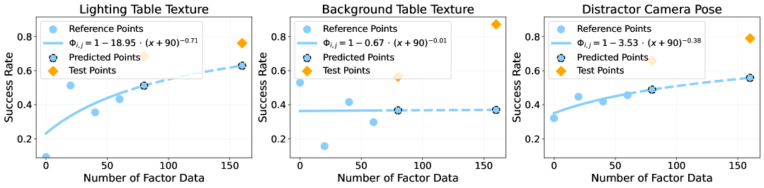
Figure 9: Factored scaling curves for the simulation Pull Cube Tool - Visual task.

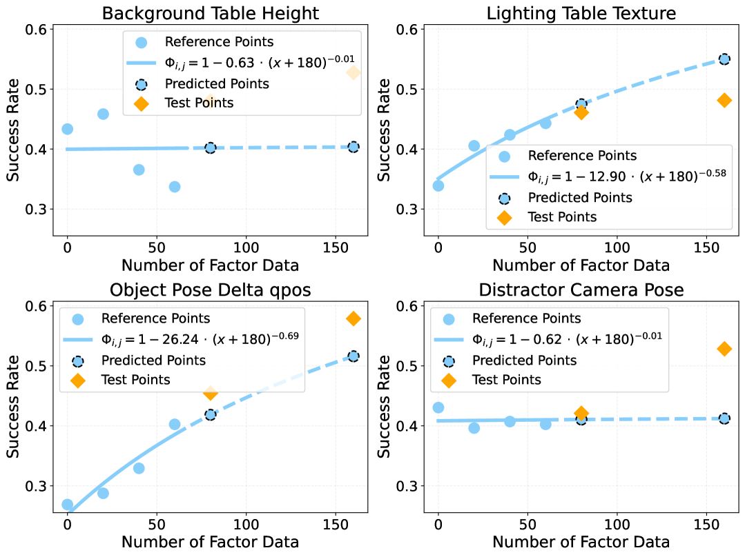
Figure 10: Factored scaling curves for the simulation Peg Insertion - Spatial task.

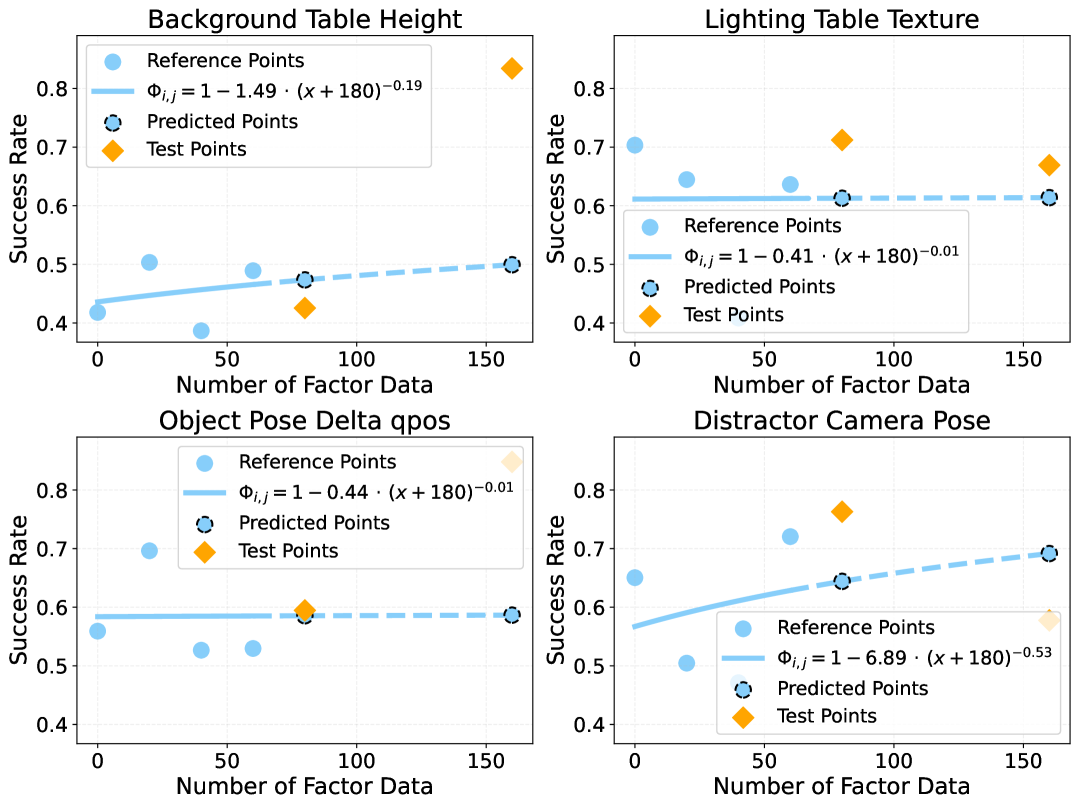
Figure 11: Factored scaling curves for the simulation Pull Cube Tool - Spatial task.

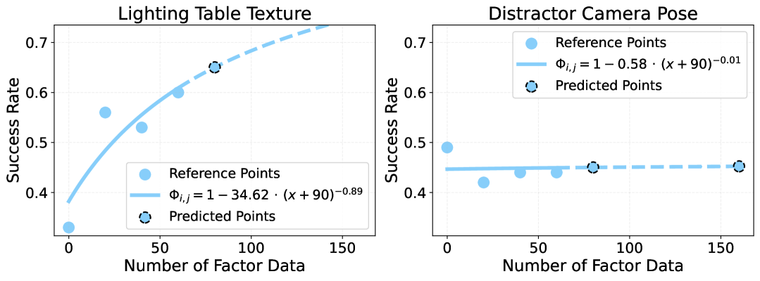
Figure 12: Factored scaling curves for the real Pick Place task. For real world tasks, we do not obtain the ground truth test points for visualization.

(a) Pick Place

(b) Peg Insertion

(c) Pull Cube Tool

Figure 13: Illustrations of simulation tasks.

Appendix B Simulation Experiments

(a) Background

(b) Distractor Objects

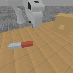
(c) Camera Pose

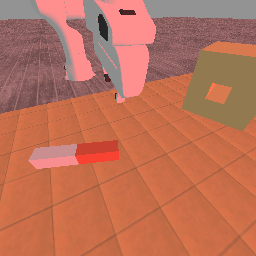
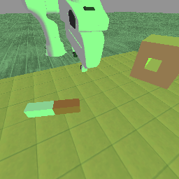
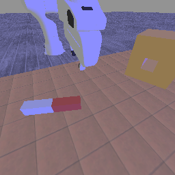
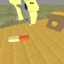
(d) Lighting

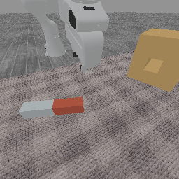
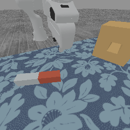
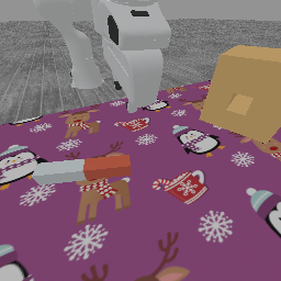
(e) Table Texture

Figure 14: Visualization of simulation environment visual factor variations.

All experiments are done in Maniskill3 [46] on a Franka Panda robot.

B.1 Task and Factor Description

We visualize all simulation tasks in Fig. 13. To collect training data, we sample continuous‑factor values according to Table 8. Note that robot pose and table height are varied only in experiments that involve spatial factors. For tasks with two cameras, we only vary the pose of the third-person view camera. The object‑pose range shown in Table 8 is used for all data except the object‑pose‑variation subset, for which we extend the range by an additional $25\%$.

For table‑texture and background variations, we draw four instances from a fixed texture dataset. We also prepare four sets of distractors for the distractor‑factor variation, each set containing two objects (e.g., eggplant, cup, cucumber). All visual factors are illustrated in Fig. 14.

Table 8: Range for each continuous factor in meters for simulation tasks.

Factor	Parameters	Pick Place	Peg Insertion	Pull Cube Tool
Manipulated object pose	X-position	$[-0.2,0.2]$	$[-0.04,0.04]$	$[-0.04,0.04]$
	Y-position	$[-0.2,0.2]$	$[-0.04,0.04]$	$[-0.08,0.08]$
	Yaw	-	$[-0.13,0.13]$	-
Goal object pose	X-position	$[-0.15,0.15]$	$[-0.04,0.04]$	$[-0.04,0.04]$
	Y-position	$[-0.2,0.2]$	$[-0.04,0.04]$	$[-0.08,0.08]$
	Yaw	-	$[-0.13,0.13]$	$[-0.13,0.13]$
Camera position	Eye-X	$[-0.05,0.05]$	$[-0.025,0.025]$	$[-0.05,0.05]$
	Eye-Y	$[-0.1,0.1]$	$[-0.025,0.025]$	$[-0.05,0.05]$
	Eye-Z	$[-0.1,0.1]$	$[-0.025,0.025]$	$[-0.05,0.05]$
Robot pose	Initial joint angles	-	$[-0.015,0.015]$	$[-0.01,0.01]$
Table height	-	-	$[-0.025,0.025]$	$[-0.025,0.025]$

Pick-Place: The robot must pick up a round toy tomato and place it onto a metal plate. Success is defined as the tomato is within $5cm$ to the center of the plate. For this task, we collect training data by replaying real-world trajectories of the real Pick Place task. We use two $192\times 192$ RGB cameras: one mounted on the wrist and one positioned off‑table, pointing at the table center. The initial dataset contains 150 demonstrations, with 30 demos per factor.

Peg Insertion: The robot must pick up a rectangular peg and insert it into a hole in a box, requiring high precision. Success is defined as half of the peg is inserted into the hole. Two $256\times 256$ RGB cameras are used: a wrist camera and a third‑person‑view camera positioned off‑table, pointing at the table center. We adapt this task from the ManiSkill3 codebase [46] and use a scripted policy to collect data. For the visual task, the initial dataset includes 150 demos (30 per factor); for the spatial task, it includes 240 demos (30 per factor).

Pull Cube Tool: The robot must first pick up an L‑shaped tool and then use it to pull a cube closer, beyond its unaided reach. Success is defined as pulling the cube to within $45,\text{cm}$ of the robot base. One $192\times 192$ RGB camera is placed off‑table, pointing at the table center. We adapt this task from the ManiSkill3 codebase [46] and use a scripted policy to collect data. For the visual task, the initial dataset contains 150 demos (30 per factor); for the spatial task, it contains 240 demos (30 per factor).

B.2 Policy Implementation Details

All policies are trained with Diffusion Policy [47]. We use ResNet-18 [49] as our vision encoder. Each policy undergoes 50000 gradient updates with a fixed batch size of 64, yielding identical computational cost across datasets of different sizes. RGB observations are augmented with standard color‑jitter during training. A complete list of hyper‑parameters is provided in Table 9.

The robot state is an 8‑dimensional vector comprising the seven joint positions and a single gripper state. Actions are specified as 8‑dimensional absolute joint‑position commands sent to a absolute position controller.

Table 9: Hyper-parameters of simulation diffusion policy.

Model Dimension	Dim Mults	Time Embedding Dimension	History Steps	Horizon	Action Steps
128	[1,2,4]	128	1	16	8

B.3 Evaluation Details

Each policy is evaluated on ten discrete settings per factor, different from the training settings. For every setting we execute 60 trials with distinct initial states, resulting in $N\times 10\times 60$ rollouts—3000 trials in the visual‑factor regime and 4800 trials in the full‑factor regime. Reported success rates are the mean over all rollouts.

Appendix C Real Robot Experiment

C.1 Hardware Setup

We use a Franka Panda robot for our real robot experiment. We use Logitech C920 webcam as our third person camera, and RealSense D405 for the wrist camera. Both cameras use resolution $192\times 192$. We use a Meta Quest 2 VR headset for teleoperation to perform data collection.

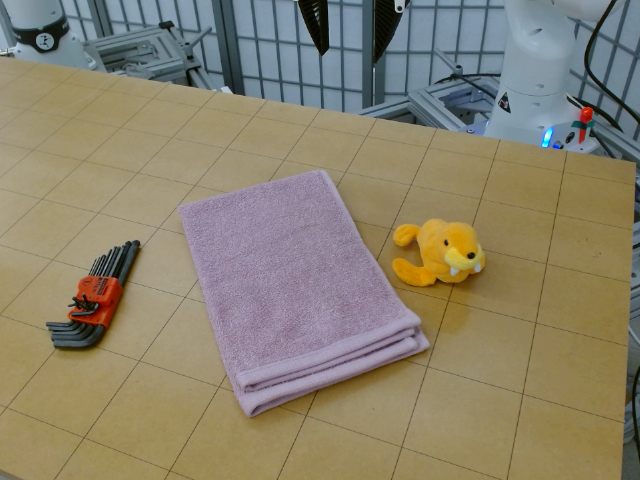
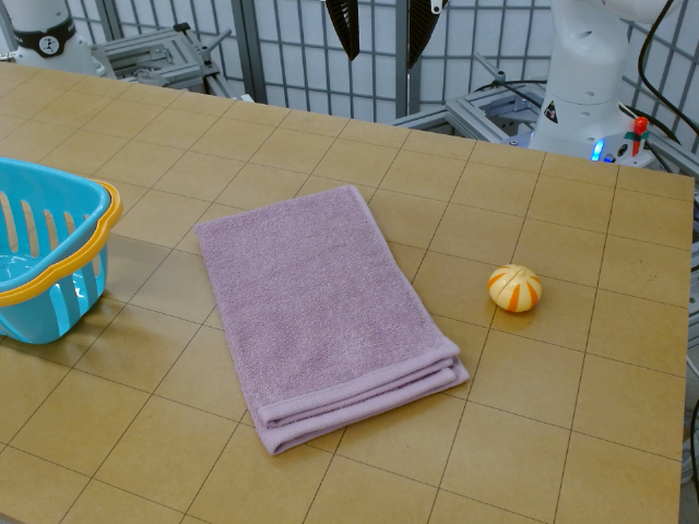
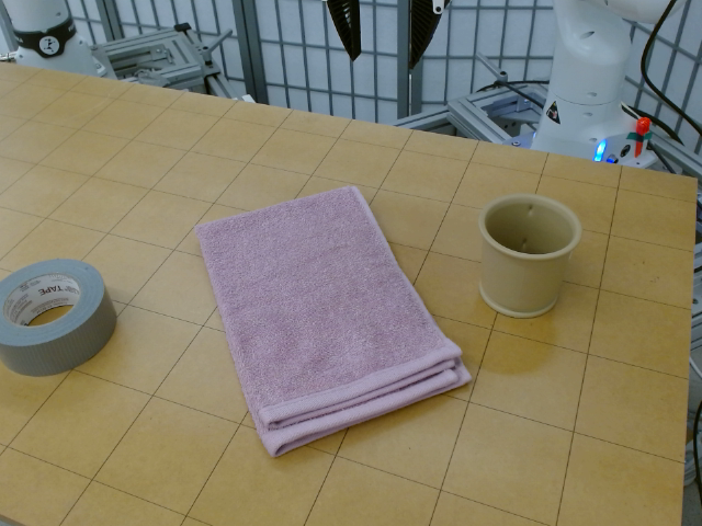
(a) Distractor Objects

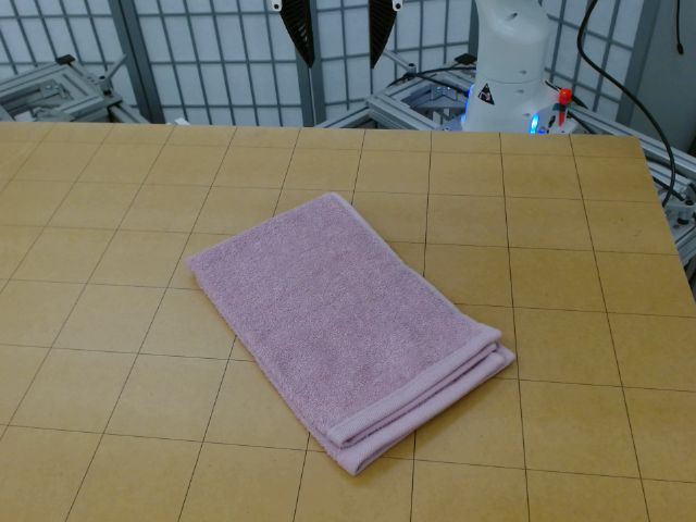
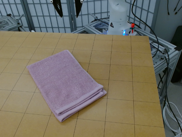
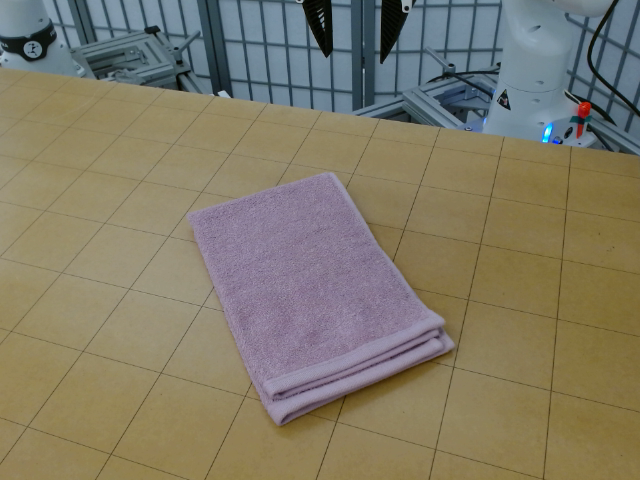
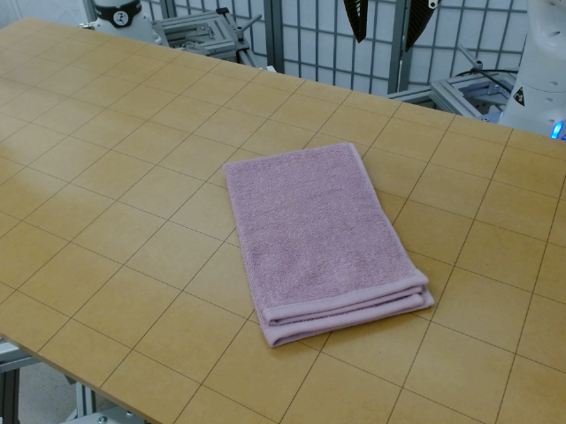
(b) Camera Pose

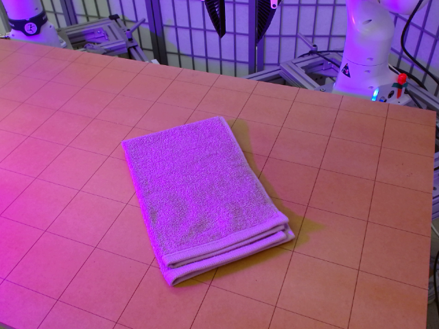
(c) Lighting

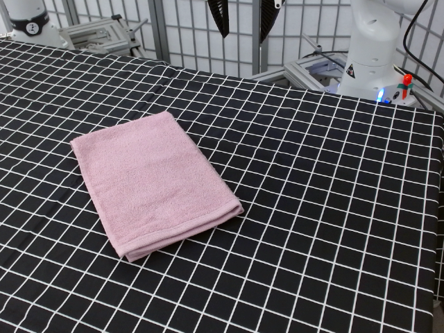
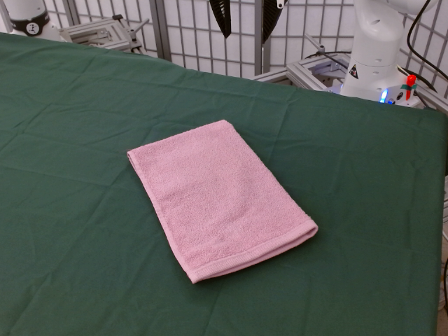
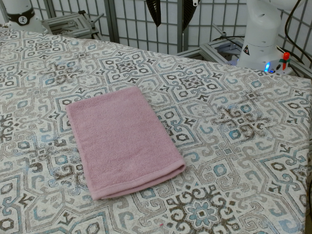
(d) Table Texture

Figure 15: Visualization of real environment factor variations.

C.2 Task and Factor Description

For training, we sample four pre-specified camera poses for the third-person camera, as visualized in Fig. 15. We use four textured and colored cloths to set up table texture variations. We use four sets of distractors for the distractor factor variation, where each set of distractor contains two objects, e.g., bread, eggplant, grape, carrot, etc. For spatial factor experiments, robot initial joint position is drawn from [-0.015,+0.015] around its nominal joint positions. Table height is omitted because it is difficult to change in our real world experiment setting. We increase the range of object pose by $25\%$ more for object pose variation. We visualize the visual factor variations in Fig. 15.

Pick place: the robot needs to pick up a round tomato and place it into a metal plate. The tomato position and the plate position and randomly set in a $40cm\times 40cm$ grid. The rotation of the plate is randomly set across training demonstrations and evaluations. We consider an initial dataset size of 120 demos, where we have 30 demos for each factor.

Fold Towel: the robot needs to grasp the end of a rectangular towel and fold it in half across the line bisecting the longer side. We collect training data with the towel position randomly set in a $5cm\times 5cm$ grid and rotation between $30^{\circ}\text{ to }60^{\circ}$ counterclockwise relative to the vertical axis. For Fold Towel - Visual, we consider an initial dataset size of 120 demos, where we have 30 demos for each factor. For Fold Towel - Spatial, we consider an initial dataset size of 180 demos, where we have 30 demos for each factor.

Mouse in Drawer: the robot needs to open a drawer, pick up a mouse, place it in the opened drawer, and close the drawer. We collect training data with drawer and mouse positions each randomly set within $\sim 10\,\text{cm}$ and rotations within $\pm 10^{\circ}$ of a fixed initial setup. We consider an initial dataset size of 180 demos, where we have 30 demos for each factor.

C.3 Policy Implementation Details

For Pick Place task, we use diffusion policy [47] to train all the policies. We follow the same color jitter augmentation protocol and hyper-parameters in Table 9.

For Fold Towel and Mouse in Drawer task, we fine-tune $\pi_{0}$ on our collected dataset. Specifically, we fine-tune from $\pi_{0}-base$ model. We freeze the ViT and the language model, and only train the action expert. We train all policies for 10,000 gradient steps for the same batch size 32, resulting in an equal training cost regardless of dataset size.

We use absolute joint position control for all the tasks. The input to the policy is camera images and a 8-dimensional state vector, consisting of robot current joint angles and gripper state. The output is a 8-dimensional vector, consisting of robot target joint angles and target gripper state. The control frequency is 15 Hz.

C.4 Evaluation Details

We evaluate each policy in difficult out-of-distribution cases where we randomly draw values for each $f_{i}$ different from the training environment.

For the Pick Place task, we evaluate each policy on 10 factor value combinations, 2 trials per combination, for 20 trails in total. We assign $0/1$ success.

For Fold Towel task, we evaluate each policy on 4 factor value combinations, 3 trials per value, for 12 trails in total. We assign partial credit, where $0$ stands for complete failure, $0.25$ stands for underfold/overfold by more than 5 centimeters or more than $20^{\circ}$, $0.5$ stands for underfold/overfold by less than 5 centimeters and less than $20^{\circ}$ but more than $3cm$ or $5^{\circ}$, and $1$ for complete success.

For Mouse in Drawer task, we evaluate each policy on 6 factor value combinations, 3 trials per value, for 18 trails in total. We assign $0$ for failing to open the drawer or pick up the mouse, $0.25$ for successfully picking up the mouse and failing to put in the drawer, $0.5$ for successfully putting the mouse into the drawer but failing to close the drawer, $1$ for complete success.

The rollout is terminated early if the robot collides with the table or enters any other hazardous state, and the trial is marked as a failure. Each rollout is capped at 600 environment steps; any trial that exceeds this limit is recorded as a failure.

C.5 Baseline Details

Re-Mix.

We train a discrete reference model with domain weights proportional to size and select the best reference model by lowest validation loss. Next, we learn the domain weights by applying robust optimization that minimizes worst case excess loss between the learned and reference policy. We take the average value of the domain weights across robust optimization training and use it for downstream policy training.

Table 10: Hyperparameters: Remix

Group	Hyperparameter	Value
Dataloader	batch size	32
Action Head (Reference)	head type	DDPMActionHead
	model class	ConditionalUnet1D
	down features	(256, 512, 1024)
	mid layers	2
	time features	128
	kernel size	5
	clip sample	1.0
	diffusion timesteps	100
	variance type	fixed small
Action Head (Remix)	head type	DiscreteActionHead
	model class	MLP
	hidden dims	(512, 512, 512)
	dropout rate	0.4
	activate final layer	True
	layer normalization	True
	number of action bins	48
	bin type	gaussian
LR Schedule (optax.warmup_cosine_decay_schedule)	initial value	$1\times 10^{-6}$
	peak value	$1\times 10^{-4}$
	warm-up steps	1 000
	decay steps	500 000
	end value	$1\times 10^{-6}$
Training / DoReMi	domain-weight step size	0.2
	smoothing	$5\times 10^{-2}$

References

- Brohan et al. [2023] A. Brohan et al. Rt-2: Vision-language-action models transfer web knowledge to robotic control, 2023. URL https://arxiv.org/abs/2307.15818.
- Black et al. [2024] K. Black et al. : A vision-language-action flow model for general robot control, 2024. URL https://arxiv.org/abs/2410.24164.
- Kim et al. [2024] M. J. Kim, K. Pertsch, S. Karamcheti, T. Xiao, A. Balakrishna, S. Nair, R. Rafailov, E. Foster, G. Lam, P. Sanketi, Q. Vuong, T. Kollar, B. Burchfiel, R. Tedrake, D. Sadigh, S. Levine, P. Liang, and C. Finn. Openvla: An open-source vision-language-action model, 2024. URL https://arxiv.org/abs/2406.09246.
- Team et al. [2025] G. R. Team et al. Gemini robotics: Bringing ai into the physical world, 2025. URL https://arxiv.org/abs/2503.20020.
- Zhao et al. [2024] T. Z. Zhao, J. Tompson, D. Driess, P. Florence, K. Ghasemipour, C. Finn, and A. Wahid. Aloha unleashed: A simple recipe for robot dexterity. arXiv preprint arXiv:2410.13126, 2024.
- Khazatsky et al. [2024] A. Khazatsky et al. Droid: A large-scale in-the-wild robot manipulation dataset. 2024.
- Walke et al. [2024] H. Walke, K. Black, A. Lee, M. J. Kim, M. Du, C. Zheng, T. Zhao, P. Hansen-Estruch, Q. Vuong, A. He, V. Myers, K. Fang, C. Finn, and S. Levine. Bridgedata v2: A dataset for robot learning at scale, 2024. URL https://arxiv.org/abs/2308.12952.
- Collaboration et al. [2024] O. X.-E. Collaboration et al. Open x-embodiment: Robotic learning datasets and rt-x models, 2024. URL https://arxiv.org/abs/2310.08864.
- Chi et al. [2024] C. Chi, Z. Xu, C. Pan, E. Cousineau, B. Burchfiel, S. Feng, R. Tedrake, and S. Song. Universal manipulation interface: In-the-wild robot teaching without in-the-wild robots, 2024. URL https://arxiv.org/abs/2402.10329.
- Kim et al. [2025] M. J. Kim, C. Finn, and P. Liang. Fine-tuning vision-language-action models: Optimizing speed and success, 2025. URL https://arxiv.org/abs/2502.19645.
- Gao et al. [2024] J. Gao, A. Xie, T. Xiao, C. Finn, and D. Sadigh. Efficient data collection for robotic manipulation via compositional generalization, 2024. URL https://arxiv.org/abs/2403.05110.
- Nguyen et al. [2025] D. Nguyen, W. Yang, R. Anand, Y. Yang, and B. Mirzasoleiman. Mini-batch coresets for memory-efficient language model training on data mixtures, 2025. URL https://arxiv.org/abs/2407.19580.
- Guruprasad et al. [2024] P. Guruprasad, H. Sikka, J. Song, Y. Wang, and P. P. Liang. Benchmarking vision, language, & action models on robotic learning tasks, 2024. URL https://arxiv.org/abs/2411.05821.
- Hejna et al. [2024] J. Hejna, C. Bhateja, Y. Jian, K. Pertsch, and D. Sadigh. Re-mix: Optimizing data mixtures for large scale imitation learning, 2024. URL https://arxiv.org/abs/2408.14037.
- Hejna et al. [2025] J. Hejna, S. Mirchandani, A. Balakrishna, A. Xie, A. Wahid, J. Tompson, P. Sanketi, D. Shah, C. Devin, and D. Sadigh. Robot data curation with mutual information estimators, 2025. URL https://arxiv.org/abs/2502.08623.
- Xie et al. [2023] S. M. Xie, H. Pham, X. Dong, N. Du, H. Liu, Y. Lu, P. S. Liang, Q. V. Le, T. Ma, and A. W. Yu. Doremi: Optimizing data mixtures speeds up language model pretraining. In Advances in Neural Information Processing Systems, 2023.
- Liu et al. [2025] Q. Liu, X. Zheng, N. Muennighoff, G. Zeng, L. Dou, T. Pang, J. Jiang, and M. Lin. Regmix: Data mixture as regression for language model pre-training, 2025. URL https://arxiv.org/abs/2407.01492.
- Lindley [1956] D. V. Lindley. On a measure of the information provided by an experiment. The Annals of Mathematical Statistics, 27(4):986–1005, 1956. ISSN 00034851, 21688990. URL http://www.jstor.org/stable/2237191.
- Chaloner and Verdinelli [1995] K. Chaloner and I. Verdinelli. Bayesian Experimental Design: A Review. Statistical Science, 10(3):273 – 304, 1995. doi:10.1214/ss/1177009939. URL https://doi.org/10.1214/ss/1177009939.
- MacKay [1992] D. J. C. MacKay. Information-based objective functions for active data selection. Neural Computation, 4(4):590–604, Jul 1992. ISSN 0899-7667. doi:10.1162/neco.1992.4.4.590. Funding by Caltech Fellowship.
- Houlsby et al. [2011] N. Houlsby, F. Huszár, Z. Ghahramani, and M. Lengyel. Bayesian active learning for classification and preference learning, 2011. URL https://arxiv.org/abs/1112.5745.
- Sener and Savarese [2018] O. Sener and S. Savarese. Active learning for convolutional neural networks: A core-set approach. In International Conference on Learning Representations, 2018.
- Anwar et al. [2025] A. Anwar, R. Gupta, Z. Merchant, S. Ghosh, W. Neiswanger, and J. Thomason. Efficient Evaluation of Multi-Task Robot Policies With Active Experiment Selection, Feb. 2025. URL http://arxiv.org/abs/2502.09829. arXiv:2502.09829 [cs].
- Kaplan et al. [2020] J. Kaplan, S. McCandlish, T. Henighan, T. B. Brown, B. Chess, R. Child, S. Gray, A. Radford, J. Wu, and D. Amodei. Scaling laws for neural language models, 2020. URL https://arxiv.org/abs/2001.08361.
- OpenAI et al. [2024] OpenAI et al. Gpt-4 technical report, 2024. URL https://arxiv.org/abs/2303.08774.
- Brown et al. [2020] T. Brown et al. Language models are few-shot learners. In Advances in Neural Information Processing Systems, 2020. URL https://proceedings.neurips.cc/paper_files/paper/2020/file/1457c0d6bfcb4967418bfb8ac142f64a-Paper.pdf.
- Hoffmann et al. [2022] J. Hoffmann, S. Borgeaud, A. Mensch, E. Buchatskaya, T. Cai, E. Rutherford, D. de Las Casas, L. A. Hendricks, J. Welbl, A. Clark, T. Hennigan, E. Noland, K. Millican, G. van den Driessche, B. Damoc, A. Guy, S. Osindero, K. Simonyan, E. Elsen, J. W. Rae, O. Vinyals, and L. Sifre. Training compute-optimal large language models, 2022. URL https://arxiv.org/abs/2203.15556.
- Grattafiori et al. [2024] A. Grattafiori et al. The llama 3 herd of models, 2024. URL https://arxiv.org/abs/2407.21783.
- Radford et al. [2021] A. Radford, J. W. Kim, C. Hallacy, A. Ramesh, G. Goh, S. Agarwal, G. Sastry, A. Askell, P. Mishkin, J. Clark, G. Krueger, and I. Sutskever. Learning transferable visual models from natural language supervision. In Proceedings of the 38th International Conference on Machine Learning, Proceedings of Machine Learning Research, 2021.
- Zhai et al. [2022] X. Zhai, A. Kolesnikov, N. Houlsby, and L. Beyer. Scaling vision transformers. In Proceedings of the IEEE/CVF Conference on Computer Vision and Pattern Recognition (CVPR), pages 12104–12113, June 2022.
- Peebles and Xie [2023] W. Peebles and S. Xie. Scalable diffusion models with transformers. In Proceedings of the IEEE/CVF international conference on computer vision, pages 4195–4205, 2023.
- Henighan et al. [2020] T. Henighan, J. Kaplan, M. Katz, M. Chen, C. Hesse, J. Jackson, H. Jun, T. B. Brown, P. Dhariwal, S. Gray, C. Hallacy, B. Mann, A. Radford, A. Ramesh, N. Ryder, D. M. Ziegler, J. Schulman, D. Amodei, and S. McCandlish. Scaling laws for autoregressive generative modeling, 2020. URL https://arxiv.org/abs/2010.14701.
- Sharma et al. [2018] P. Sharma, L. Mohan, L. Pinto, and A. Gupta. Multiple interactions made easy (mime): Large scale demonstrations data for imitation. In Conference on robot learning, pages 906–915. PMLR, 2018.
- Kalashnikov et al. [2018] D. Kalashnikov, A. Irpan, P. Pastor, J. Ibarz, A. Herzog, E. Jang, D. Quillen, E. Holly, M. Kalakrishnan, V. Vanhoucke, et al. Scalable deep reinforcement learning for vision-based robotic manipulation. In Conference on robot learning, pages 651–673. PMLR, 2018.
- Cabi et al. [2020] S. Cabi, S. G. Colmenarejo, A. Novikov, K. Konyushkova, S. Reed, R. Jeong, K. Zolna, Y. Aytar, D. Budden, M. Vecerik, O. Sushkov, D. Barker, J. Scholz, M. Denil, N. de Freitas, and Z. Wang. Scaling data-driven robotics with reward sketching and batch reinforcement learning, 2020. URL https://arxiv.org/abs/1909.12200.
- Lin et al. [2024] F. Lin, Y. Hu, P. Sheng, C. Wen, J. You, and Y. Gao. Data scaling laws in imitation learning for robotic manipulation, 2024. URL https://arxiv.org/abs/2410.18647.
- Belkhale et al. [2023] S. Belkhale, Y. Cui, and D. Sadigh. Data quality in imitation learning, 2023. URL https://arxiv.org/abs/2306.02437.
- Liu et al. [2023] H. Liu, S. Nasiriany, L. Zhang, Z. Bao, and Y. Zhu. Robot learning on the job: Human-in-the-loop autonomy and learning during deployment. In Robotics: Science and Systems (RSS), 2023.
- Cui et al. [2023] Y. Cui, S. Karamcheti, R. Palleti, N. Shivakumar, P. Liang, and D. Sadigh. No, to the right: Online language corrections for robotic manipulation via shared autonomy. In Proceedings of the 2023 ACM/IEEE International Conference on Human-Robot Interaction, HRI ’23, page 93–101. ACM, Mar. 2023. doi:10.1145/3568162.3578623. URL http://dx.doi.org/10.1145/3568162.3578623.
- Gandhi et al. [2022] K. Gandhi, S. Karamcheti, M. Liao, and D. Sadigh. Eliciting compatible demonstrations for multi-human imitation learning, 2022. URL https://arxiv.org/abs/2210.08073.
- Majumdar et al. [2025] A. Majumdar, M. Sharma, D. Kalashnikov, S. Singh, P. Sermanet, and V. Sindhwani. Predictive red teaming: Breaking policies without breaking robots, 2025. URL https://arxiv.org/abs/2502.06575.
- Kaplan et al. [2020] J. Kaplan, S. McCandlish, T. Henighan, T. B. Brown, B. Chess, R. Child, S. Gray, A. Radford, J. Wu, and D. Amodei. Scaling laws for neural language models. arXiv preprint arXiv:2001.08361, 2020.
- Clauset et al. [2009] A. Clauset, C. R. Shalizi, and M. E. Newman. Power-law distributions in empirical data. SIAM review, 51(4):661–703, 2009.
- Salton et al. [1975] G. Salton, A. Wong, and C. S. Yang. A vector space model for automatic indexing. Commun. ACM, 18(11):613–620, Nov. 1975. ISSN 0001-0782. doi:10.1145/361219.361220. URL https://doi.org/10.1145/361219.361220.
- Mikolov et al. [2013] T. Mikolov, K. Chen, G. Corrado, and J. Dean. Efficient estimation of word representations in vector space, 2013. URL https://arxiv.org/abs/1301.3781.
- Tao et al. [2024] S. Tao, F. Xiang, A. Shukla, Y. Qin, X. Hinrichsen, X. Yuan, C. Bao, X. Lin, Y. Liu, T. kai Chan, Y. Gao, X. Li, T. Mu, N. Xiao, A. Gurha, Z. Huang, R. Calandra, R. Chen, S. Luo, and H. Su. Maniskill3: Gpu parallelized robotics simulation and rendering for generalizable embodied ai. arXiv preprint arXiv:2410.00425, 2024.
- Chi et al. [2023] C. Chi, S. Feng, Y. Du, Z. Xu, E. Cousineau, B. Burchfiel, and S. Song. Diffusion policy: Visuomotor policy learning via action diffusion. In Proceedings of Robotics: Science and Systems (RSS), 2023.
- Xue et al. [2025] Z. Xue, S. Deng, Z. Chen, Y. Wang, Z. Yuan, and H. Xu. Demogen: Synthetic demonstration generation for data-efficient visuomotor policy learning. arXiv preprint arXiv:2502.16932, 2025.
- He et al. [2015] K. He, X. Zhang, S. Ren, and J. Sun. Deep residual learning for image recognition, 2015. URL https://arxiv.org/abs/1512.03385.
- Du et al. [2023] M. Du, S. Nair, D. Sadigh, and C. Finn. Behavior retrieval: Few-shot imitation learning by querying unlabeled datasets. arXiv preprint arXiv:2304.08742, 2023.
- Di Palo and Johns [2024] N. Di Palo and E. Johns. On the effectiveness of retrieval, alignment, and replay in manipulation. IEEE Robotics and Automation Letters, 9(3):2032–2039, 2024.