Transfer Learning Across Fixed-Income Product Classes
Abstract
We propose a framework for transfer learning of discount curves across different fixed-income product classes. Motivated by challenges in estimating discount curves from sparse or noisy data, we extend kernel ridge regression (KR) to a vector-valued setting, formulating a convex optimization problem in a vector-valued reproducing kernel Hilbert space (RKHS). Each component of the solution corresponds to the discount curve implied by a specific product class. We introduce an additional regularization term motivated by economic principles, promoting smoothness of spread curves between product classes, and show that it leads to a valid separable kernel structure. A main theoretical contribution is a decomposition of the vector-valued RKHS norm induced by separable kernels. We further provide a Gaussian process interpretation of vector-valued KR, enabling quantification of estimation uncertainty. Illustrative examples demonstrate that transfer learning significantly improves extrapolation performance and tightens confidence intervals compared to single-curve estimation.
Keywords: yield curve estimation, transfer learning, nonparametric estimator, machine learning in finance, vector-valued reproducing kernel Hilbert space
JEL Classification: C14, E43, G12
1 Introduction
We introduce a framework for transfer learning of discount curves across different fixed-income product classes. Since discount curves are inherently unobservable, they must be inferred from the observable prices of fixed-income instruments. A key feature of the proposed framework is its ability to incorporate complementary market information across product classes. Accurate estimation is critical, as discount curves are fundamental to finance, providing the basis for appropriately discounting future cash flows. Consequently, their precise estimation holds significant practical relevance.
Numerous methods have been proposed for single discount curve estimation. Classical approaches include the parametric Nelson–Siegel–Svensson model [NS87, Sve94, GSW07], as well as nonparametric methods such as Fama–Bliss [FB87], Smith–Wilson [SW01], and Liu–Wu [LW21]. More recently, [FPY24] introduced a kernel ridge regression (KR) framework, providing a theoretically grounded solution based on reproducing kernel Hilbert space (RKHS) theory. KR yields a closed-form, linear estimator and empirically outperforms benchmark models for U.S. and Swiss government bonds [FPY24, CF24]. However, like other methods, KR struggles with extrapolation in maturity ranges where data are sparse or absent [CF24].
This limitation motivates the use of transfer learning [WKW16, PY10], a well-established concept in machine learning that is closely related to multitask learning [Car97]. Transfer learning seeks to improve estimation by jointly solving related problems and sharing information across them, particularly when data for the primary task are limited, noisy, or costly to obtain. In the context of discount curves, transfer learning arises naturally across fixed-income product classes, with suitable adjustment for cross-currency effects. A product class refers to a group of fixed-income instruments priced using a common discount curve, denominated in the same currency and characterized by similar risk features such as issuer type, collateralization, or credit quality. Examples include government bonds issued by the same sovereign, interest rate swaps referencing a common overnight risk-free rate [SS19, SIX, MM, ECB, BoEa, Fed], and corporate bonds within a given credit rating class.
This paper develops a theoretical framework for transfer learning of discount curves, complemented by illustrative examples.333Two comprehensive empirical studies are in progress, one focusing on government bonds and swaps within the same currency and the other on government bonds across currencies. Our methodology generalizes to any set of fixed-income products that can be represented jointly under a discounted cash flow framework. Although limits to arbitrage may cause different product classes to imply distinct discount curves even when all are considered risk-free [WJ24], we show that the discounted cash flow principle can be naturally embedded into an arbitrage-free pricing framework.
We formulate the transfer learning problem as a vector-valued KR, leading to a convex optimization problem in a vector-valued RKHS. Each component of the solution corresponds to the discount curve implied by a specific product class. Analogous to the scalar case, we derive a closed-form expression for the vector-valued KR estimator.
The theory of vector-valued RKHS is well-established [PR16, MP05], with operator-valued kernels, such as matrix-valued kernels in , playing a central role [KDP+16]. Fundamental results from RKHS theory, including the representer theorem and Moore’s theorem, extend naturally to the vector-valued setting [PR16]. A particularly tractable subclass, separable kernels, has been extensively studied [BRBV12, She08, MP04, ARL12]. Separable kernels are constructed as the product of a scalar kernel and a constant covariance matrix, the latter encoding the transfer learning structure. They offer computational advantages, including simple computation of inner products and induced norms [BRBV12].
Building on the scalar case, we introduce an additional regularization term motivated by economic principles, penalizing the spread between discount curves across product classes. A main theoretical contribution of our work is a decomposition of the norm induced by separable kernels, generalizing a result from [BRBV12]. We prove that the resulting regularization yields a valid separable kernel, specifically tailored to our transfer learning problem. Rather than enforcing identical curves, the regularization promotes smoothness of spread curves under an economically motivated norm. This connects naturally to graph regularization techniques [SK03, She08].
We further provide a Gaussian process [CWG19] interpretation of the vector-valued KR, enabling quantification of estimation uncertainty for the discount curves. In doing so, we extend the well-known correspondence between KR and Gaussian processes in the scalar case [RW05] to the setting of transfer learning. Our illustrative examples show that the transfer learning framework significantly tightens confidence intervals around the estimated discount curves.
The remainder of the paper is organized as follows. Section 2 formulates the transfer learning problem for discount curves and presents the representation theorem essential for implementation. Section 3 develops the Gaussian process perspective. Section 4 introduces separable kernels as a natural class of matrix-valued kernels for our setting. Section 5 discusses how standard fixed-income products can be embedded into the transfer learning formulation. Section 6 presents illustrative examples, focusing on transfer learning between government bonds and swaps. The appendix provides a self-contained introduction to the theory of vector-valued RKHS, collects all proofs, and details the embedding of the discounted cash flow principle into an arbitrage-free pricing framework. An online appendix includes additional examples.
2 Transfer learning problem formulation
In this section, we present the general problem formulation for transfer learning of discount curves across different fixed-income product classes. Our framework requires only that the theoretical price of a fixed-income product be expressed as the sum of its discounted cash flows.
Specifically, for every product class , there are fixed-income securities with common cash flow dates , stacked into the column vector .444Cash flow dates are assumed to be common across all product classes without loss of generality. The total number of securities is given by . For each security we observe noisy ex-coupon prices, . We denote the associated cash flow matrix by where is the cash flow of security of product class that occurs in .
In line with the discounted cash flow principle, we assume that for every product class , there exists a unique discount curve with and such that the price of every instrument in product class is given by
| (1) |
The objective of this paper is to jointly estimate the discount curves from observed market prices . To this end, we decompose each curve as the sum of an exogenous prior function and a hypothesis function , that is,
Here, the prior is assumed to satisfy , and the hypothesis is constrained to satisfy .555This additive specification mirrors the structure of linear-rational term structure models; see [FLT17]. A natural and simple choice for the prior is the constant function .
We model as an element of a vector-valued RKHS over the domain , taking values in and satisfying for all . The associated reproducing kernel is a matrix-valued function . Appendix A provides a self-contained introduction to the theory of vector-valued RKHS, including its foundational properties and practical relevance for our setting.
To enable matrix notation, we introduce the following conventions. For any function , we write for the corresponding array of function values. For a general matrix , we write for its -th row vector, and define the vectorization of as the vector obtained by stacking its columns, . Accordingly, we denote the matrix , and we obtain the vector
We also stack the cash flow matrices and price vectors across product classes as
where is block diagonal with the individual cash flow matrices along the diagonal, and all off-diagonal blocks equal to zero. The discounted cash flow equation (1) then reads . Including pricing errors leads to
| (2) |
Such pricing errors occur due to market imperfections and data errors.
The estimation objective reduces to finding a function that balances the tradeoff between the weighted mean-squared pricing error,
and the regularity of , as quantified by the vector-valued RKHS norm . The weights are exogenously specified and reflect the relative importance of the pricing terms. This setup corresponds to a vector-valued KR. The regularity penalty depends on the choice of the matrix-valued kernel , whose structure is encoded in the kernel matrix
| (3) |
where each block has entries . The following theorem formalizes this formulation.
Theorem 2.1.
The unique solution of the vector-valued KR problem
| (4) |
is given by where takes the form
for the block diagonal matrix with . The corresponding discount curves are given by .
A common choice for the weights is based on the duration of the underlying securities; see Section 6.2 for details. The choice of the kernel is critical, as it should be both economically meaningful and computationally tractable. In our implementation, we use a separable kernel of the form , where is a symmetric positive semi-definite matrix and is a scalar-valued kernel. This form decouples the dependence on product class, captured by the matrix , from the time-to-maturity dependence, captured by . For further background on separable kernels and their properties, we refer to Appendix A.
Remark 2.2.
Remark 2.3.
Theorem 2.1 remains valid even when no quotes are available for a given product class , i.e., when . In this case, the corresponding rows in and are omitted, and we adopt the convention that . Remarkably, the solution curve still depends on the other product classes via the joint regularization term. In the extreme case where no quotes are available at all, , the solution is identically zero, and the resulting discount curve reduces to the prior, .
3 Gaussian process view
Similar to the scalar case one can develop a Gaussian process perspective of the kernel ridge regression in the vector-valued case. We first discuss the general case and then specialize to separable kernels.
3.1 Vector-valued Gaussian processes
We recap the theory of vector-valued Gaussian processes and prove the equivalence of the posterior mean function and the vRK solution. We denote by the multivariate normal distribution with mean vector and covariance matrix .
Definition 3.1 (vector-valued Gaussian process).
We say is a vector-valued Gaussian process with mean function and kernel function if and only if for any
with and as in (3). In this case we write .
Remark 3.2.
There is no restriction to use across all components of . One can formulate a Gaussian process for any finite collection of points , , such that .
We replicate the results [FPY24, Section A.4] for the vector-valued case which is straightforward. For this we assume that is a vector-valued Gaussian process with mean function and kernel function , i.e., . The pricing equation with errors is given by equation (2) where we assume with
for symmetric positive definite -matrices .
For arbitrary cash flow dates this implies that and are jointly Gaussian distributed
| (5) |
where is the block matrix with entries , similar for such that .
Bayesian updating implies that the conditional distribution of , given the observed prices , is still vector-valued Gaussian with posterior mean function
| (6) |
with
| (7) |
and posterior kernel function
Hence we recovered the following vector-valued version of [FPY24, Lemma 9].
Theorem 3.3.
The posterior mean is invariant with respect to scaling of and by a factor . That is to replace by and . Similar as in [FPY24] one can use (5) to derive at a prior log-likelihood function of given prices
for and . The maximum log-likelihood is attained for
Remark 3.4.
When for all the posteriori mean estimator corresponds to independent scalar learned mean estimators. This can be seen from (7) as in this case the block diagonal structure of factors through, given that the matrices and are blockdiagonal by definition. However, the confidence bands might differ as does. In the scalar case the optimal scaling is given by , for the respective value . On the other hand, for the transfer learning case it holds by definition , and implies . Hence in general the scaling factors differ, , for individual classes .
3.2 Gaussian process view for separable kernels
The Gaussian process view reveals some additional interpretation for separable kernels. In particular, one can use the theory of Gaussian matrix variate distributions to get some additional insights how different components of are correlated to each other. The key findings are given below. We first recall the definition and some basic properties of matrix variate Gaussian distributions.
Definition 3.5.
The random matrix is said to have a matrix variate Gaussian distribution with mean matrix , covariance matrices and if and only if the probability density function is given by
We denote a matrix variate Gaussian distributed as .
It holds that if and only if , see [CWG19, Theorem 2]. This again implies that the transpose , see [CWG19, Theorem 1]. Hence, in view of Definition 3.1, for a separable kernel , we have that is equivalent to for and , and where denotes the matrix with entries .
This leads to a natural interpretation of the variance and covariance structure of the discount curves. From the above, we obtain and . The separable kernel structure allows us to interpret each entry as the covariance between product classes and , scaled by the scalar kernel , which reflects the time-to-maturity effect and is independent of the product class. The correlation is obtained by normalization. More details and a general decomposition result for matrix-valued kernels are provided in Lemmas A.8 and A.9 in the appendix.
4 A workable class of separable kernels
In this section, we introduce the baseline model used for both theoretical analysis and empirical implementation. The formulation is motivated by economic reasoning and results in a tractable optimization problem with a closed-form solution. It extends the single-curve model of [FPY24] to the vector-valued case. We proceed in two steps. First, we heuristically construct a joint estimation objective that includes spread penalties between curves. Second, we show that the resulting problem is equivalent to a vector-valued KR with a separable matrix-valued kernel.
We begin with scalar-valued estimation problems, each for a fixed-income product class ,
where is a common scalar kernel with RKHS , and is the regularity parameter for class . Each problem yields an individual estimator . Estimating the curves independently is equivalent to solving the joint optimization problem
This can be viewed as a single objective over the product space .
To introduce dependencies across product classes, we extend the regularization to the differences between curves. Specifically, we add spread penalties of the form
where controls the strength of transfer learning between classes and .666We also considered adjusting the individual regularization parameters downward to keep the total regularization weight constant when adding spread penalties. This corresponds to choosing in (4). However, in our empirical studies we found that such scaling can introduce irregularities in the estimated discount curves, which is undesirable. We therefore recommend keeping the values of fixed and setting to achieve a well-balanced and effective transfer learning outcome, as stated in Theorem 4.1. These terms encourage similarity between curves without forcing equality. Instead, they penalize irregularities in the spread curves through the RKHS norm . We use the terms regularity and smoothness interchangeably, referring specifically to the notion of smoothness induced by the RKHS norm . In [FPY24], a specific kernel is proposed that encodes economically meaningful smoothness properties for discount curves. We adopt this kernel specification in our implementations, see (14) and (15) below.
The complete transfer learning problem is
| (8) |
The following theorem shows that (8) can be interpreted as a vector-valued KR with a separable kernel. This implies in particular that the optimization problem is convex and admits a unique solution.
Theorem 4.1.
5 Standard fixed-income products
This section shows how standard fixed-income instruments can be expressed in the discounted cash flow format (1), thereby enabling application of our estimation framework. While this formulation may lead to distinct discount curves across different product classes, we demonstrate in Appendix C how, under an arbitrage-free pricing framework, a single risk-free curve and the corresponding function may be recovered.
We proceed as follows: we first show how coupon bonds can be cast into the pricing format (1), then extend this formulation to fixed–floating interest rate swaps. Finally, we examine cross-currency swaps and show how transfer learning facilitates joint estimation of discount curves and forward exchange rates, offering insights into multi-currency pricing.
5.1 Coupon bonds
The transformation of fixed-coupon bonds into the discounted cash flow format (1) is straightforward. Consider a bond with notional normalized to one and coupons paid at dates , where denotes the bond’s maturity at which the notional is paid.777The generic time grid used in (1) is assumed to be fine enough to cover all potential cash flow dates across product classes. Hence, most entries in each row of are zero. Assuming the bond is default-free, the price is given by
Defaultable bonds are treated in Appendix C under an arbitrage-free pricing framework.
5.2 Interest rate swaps
We consider a standard fixed–floating interest rate swap with start (first reset) date and maturity date . We denote the reset and cash flow dates of the fixed payments leg by and of the floating payments leg by . For simplicity, the accrual periods along both legs are assumed to be constant and denoted by and , respectively.888This can be generalized to specific day count conventions for both legs where the accrual periods depend on the actual dates, replacing the constant and by ) and , respectively. The swap is spot starting when and forward starting when .
The present values of the fixed and floating legs are given by
where denotes the corresponding fixed swap rate. At inception, the swap has zero value, so that . We bring this into the desired format (1) as follows. For a spot-starting swap, , the price is set to , which gives
| (11) |
For a forward-starting swap, , the price is set to , which gives
| (12) |
5.3 Cross-currency swaps
Cross-currency swaps (XCCY) involve cash flows in two currencies and combine features of both interest rate and foreign exchange (FX) instruments. See, e.g., [Ran23, BHJ+19] for introductions. We denote the spot exchange rate prevailing at time as , defined as the price of one unit of (base) currency in terms of (quote) currency .
A typical use case involves a domestic, say Swiss, firm that holds CHF and wishes to buy a USD-denominated bond. To hedge currency risk, the firm enters a XCCY swapping USD coupon payments against CHF cash flows.999Another example is two firms located in different countries with different currencies. Each exhibits cheaper local funding sources. To raise funds abroad they can enter into a bilateral XCCY.
The most standardized and actively traded XCCY is the floating–floating type used in the interbank market. At the start date , notional amounts in both currencies are exchanged at the prevailing spot exchange rate . Thereafter, floating interest payments are made in each currency at dates , typically quarterly and based on overnight risk-free rates (RFRs). The initial notional amounts are re-exchanged at maturity date . A basis spread is typically added to the less liquid currency leg to reflect liquidity differences and funding imbalances between the two currencies. Figure 1 illustrates this.
An additional feature common in interbank markets is mark-to-market (MTM) resets of the notional leg. These reduce counterparty risk but, as shown in Appendix C, have no impact on present values.
End clients generally prefer fixed interest payments. Banks accommodate this by combining floating–-floating XCCY with standard fixed–floating interest rate swaps. This composite structure is also necessary for estimating the discount curve using our framework. We focus on the non-liquid leg (currency ), and bring this now into the desired format (1). Thereto, let be the fixed swap rate of a standard RFR-based swap in currency with the same maturity as the XCCY. We assume this rate is observable from the market.101010This is standard practice in well-developed swap markets. More specifically, let be the fixed leg’s payment dates with constant accrual period , and assume that currency is the more liquid leg, so the basis spread is added to leg . For a spot-starting XCCY, , we set . The corresponding discounted cash flow equation becomes
For a forward-starting XCCY, , the price is set and we obtain
Here, denotes the discount curve for currency induced by currency via an XCCY. It incorporates the cross-currency basis and is generally distinct from the discount curve that corresponds to standard interest rate swaps in currency . If the basis spread is zero, coincides with .
An important byproduct of this formulation is an expression for the forward exchange rate that incorporates the cross-currency basis. Let denote the forward exchange rate fixed at time for maturity . Then
| (13) |
This identity can be derived by considering a spot-starting XCCY in combination with an interest rate swap with a single payment at . Investing one unit of currency via this XCCY and swapping the floating payment for fixed results in a fixed payoff of units of currency at maturity . Alternatively, the same initial amount can be used to purchase units of the discount bond with maturity in currency . At maturity, this yields a cash flow in currency , which is then converted back into currency at the forward exchange rate , resulting in a payoff of in currency . Since both strategies yield deterministic payoffs, the absence of arbitrage implies that they must be equal, which proves (13).
Remark 5.1.
Textbook covered interest parity (CIP) posits that . However, in practice, deviations from CIP are persistent, as due to liquidity differences and funding constraints. Most currencies exhibit a negative basis against USD, meaning counterparties are willing to accept a lower return to obtain USD funding, which manifests as in observed XCCY swaps.
6 Implementation and examples
This section illustrates the effects of transfer learning through a series of representative examples. While not intended as a full empirical study, these examples demonstrate the model’s behavior in realistic scenarios. We focus on transfer learning across product classes, government bond and RFR-based swaps within the same currency, for four currencies. We first introduce the data, followed by a description of the base model and implementation details. We conclude with an illustration of the effects of transfer learning.
6.1 Data
We source data of government bonds and RFR-based swaps from Bloomberg111111Bloomberg Finance L.P. for four currencies, CHF, EUR, GBP, and USD, on five representative business days of the years 2020 to 2024. Following the approach in [CF24], we select the mid-June (nearest available) business day of each year: 2020-06-15, 2021-06-15, 2022-06-15, 2023-06-15, and 2024-06-14.
For government bonds, we use dirty prices, assuming same-day settlement. Our selection includes all fully taxable, non-callable coupon bonds, applying filters consistent with [FB87, LW21]. Following [GSW07], we exclude bonds with fewer than 90 days to maturity and omit all bills. The CHF market has the smallest number of bonds, while the USD market has the largest. Maturity distributions vary across markets. CHF and GBP markets contain bonds with maturities over 40 and 50 years, respectively. EUR and USD maturities initially extend to about 35 years, tapering to around 30 years. Overall, maturity coverage is denser in USD and EUR.
Swap data consists of rates for standard fixed–floating interest rate swaps, where the floating leg is linked to transaction-based overnight RFRs [SS19]. For Switzerland, the reference rate is the Swiss Average Rate Overnight (SARON) [SIX], which is collateralized. In the euro area, two benchmarks exist: EURIBOR and the Euro Short-Term Rate (ESTR) [ECB]. We use ESTR, which is unsecured but still considered risk-free. In the UK, the reformed RFR is the Sterling Overnight Index Average (SONIA) [BoEb], also unsecured. In the U.S., the Secured Overnight Financing Rate (SOFR) [Fed] serves as the RFR and is collateralized. The number of available swap tenors is broadly comparable across currencies, ranging from overnight to 50 years. Both ESTR and SONIA tenors even extend to 60 years.
6.2 Base model and implementation details
To implement the KR estimator in (4), we adopt duration-based weights , as commonly used in the literature; see, e.g., [FPY24, CF24]. For any fixed-income instrument with cash flows at dates , its price as a function of yield-to-maturity (YTM) is given by
The market-implied YTM is defined by , where denotes the observed market price. The model-implied YTM , based on a discount curve , satisfies , consistent with the discounted cash flow equation (1). Using a first-order approximation, , we express the squared YTM error as an approximately weighted squared price error,
YTM is often used to compare fixed-income instruments across maturities. Weighting squared price errors by therefore ensures that estimation errors are more uniformly comparable across the maturity spectrum.
This logic also applies to swaps, for which either (spot-starting) or (forward-starting). The following result links YTM to the swap rate :
Lemma 6.1.
If for all , then . That is, in first order the YTM equals the swap rate, .
The following example illustrates this for a single-period overnight swap.
Example 6.2.
In the U.S., the overnight RFR is SOFR, here denoted by . Consider a single-period overnight swap maturing at . The pricing equation (11) here is . The corresponding YTM satisfies
which implies
The derivative of the YTM–price function is , so the corresponding duration-based weight becomes .
We use the separable kernel from Theorem 4.1 with scalar kernel given by
| (14) |
for a maturity weight parameter , which is introduced in [FPY24].121212The RKHS introduced in [FPY24] is more flexible, as its norm (15) includes both first- and second-order derivatives. However, their empirical analysis on U.S. data finds that only the second-order term is relevant for the performance of the KR estimator. [CF24] confirm this finding for Swiss data as well. They show that the corresponding RKHS is the weighted Sobolev space consisting of twice weakly differentiable functions with , , and finite smoothness norm given by
| (15) |
In sum, this specification includes the following hyperparameters: (scalar kernel parameter), (discount curve smoothness), (spread smoothness). To reduce complexity, we set for all and for all .
We set and , as calibrated in [FPY24] for U.S. data.131313In fact, [FPY24] use for the prevailing last maturity date , although the differences are economically negligible. [CF24] find that and are statistically optimal for Swiss data. However, they also show that variations in and within this range have no economically significant impact on the KR estimation. The remaining tuning parameter is , which governs the strength of transfer learning. We consider values . Setting corresponds to independent estimation without transfer learning.
6.3 Illustrative effects of transfer learning
To demonstrate the effects of transfer learning, we present two representative examples in the main text: EUR and USD market, both for the date 2024-06-14. For size reasons, we show only these two instances here. The full set of results across all currencies and dates is provided in the supplementary online appendix.141414Available at Online Appendix for Transfer Learning Across Fixed-Income Product Classes.
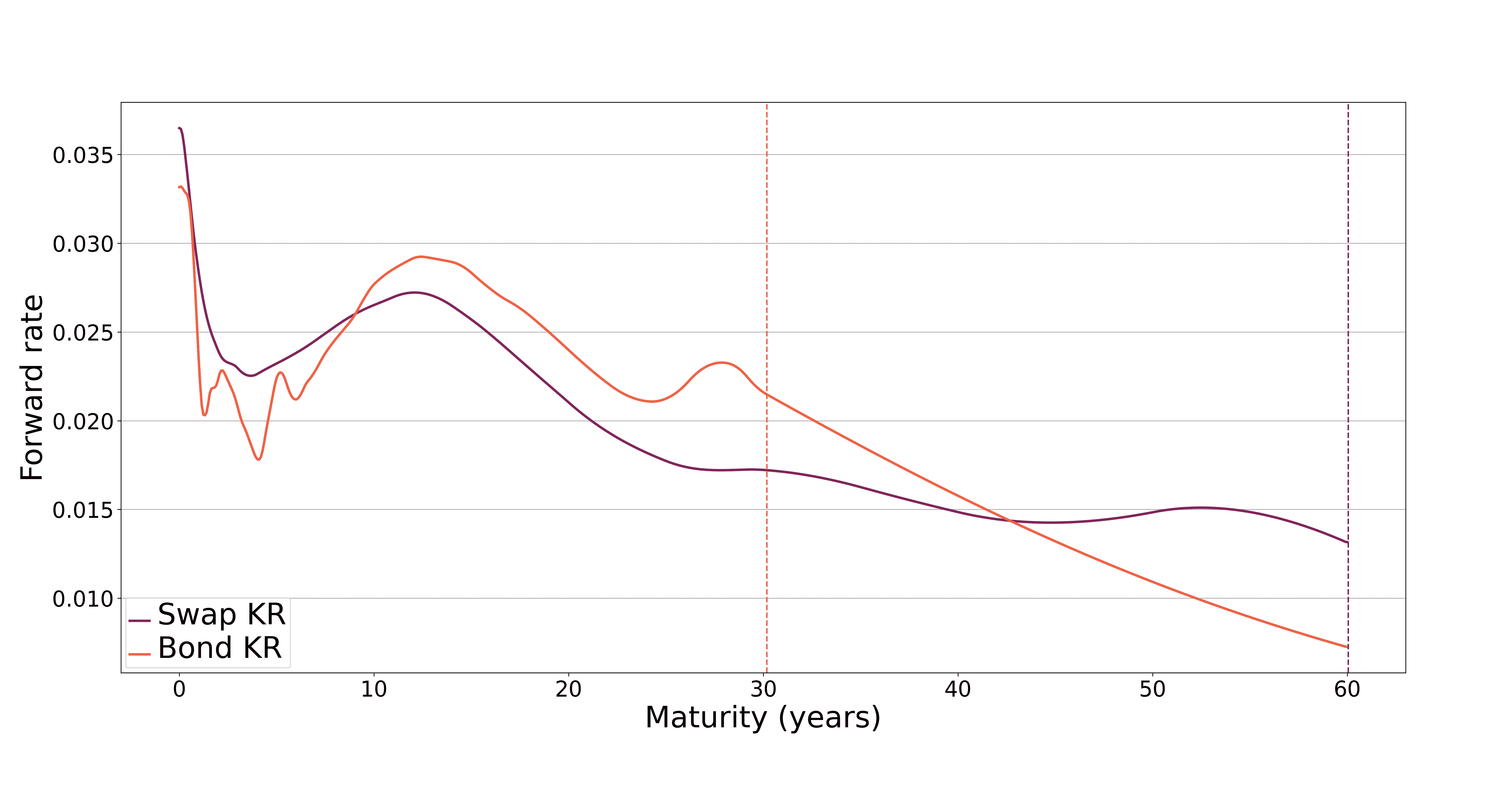
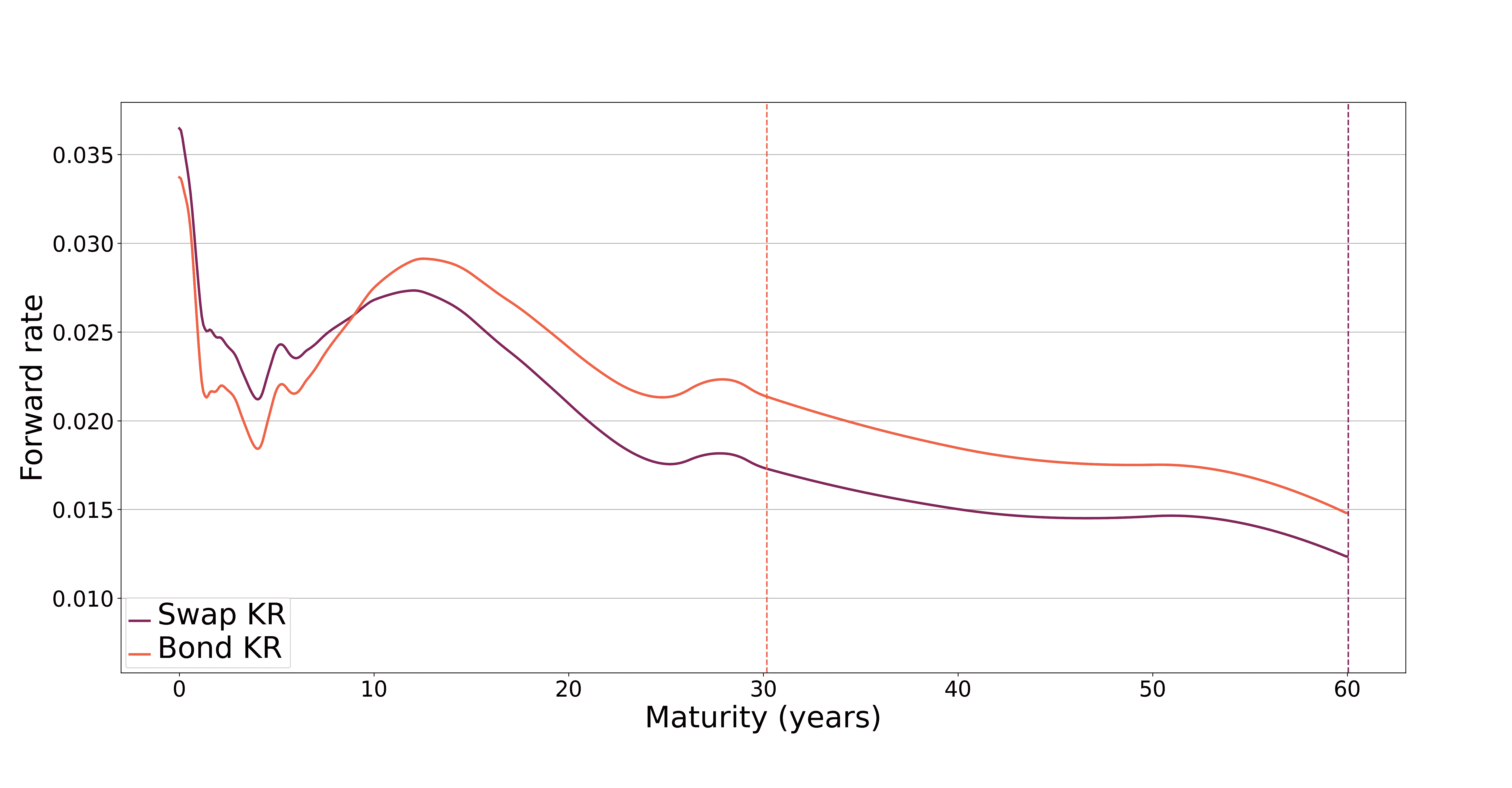
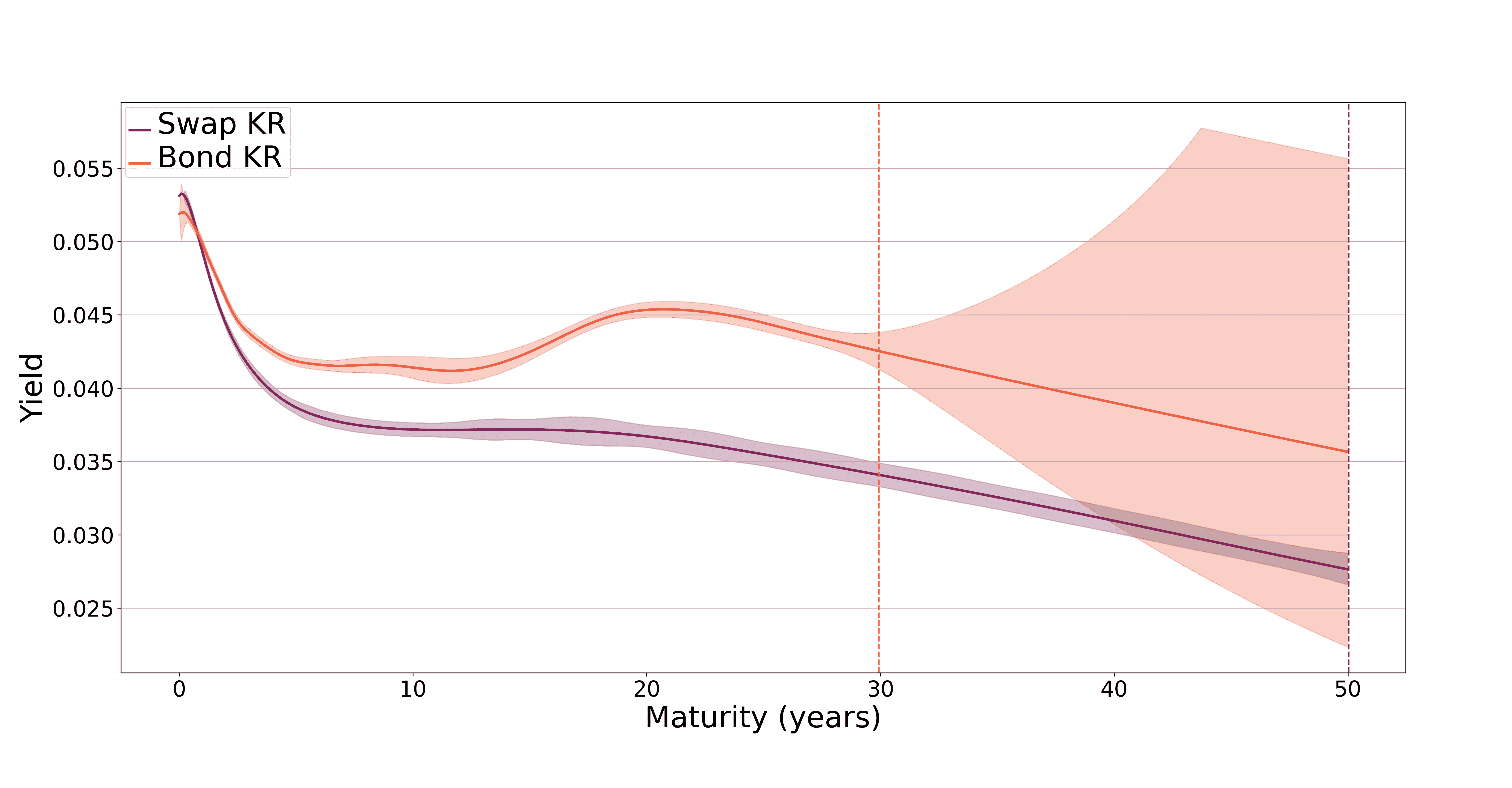
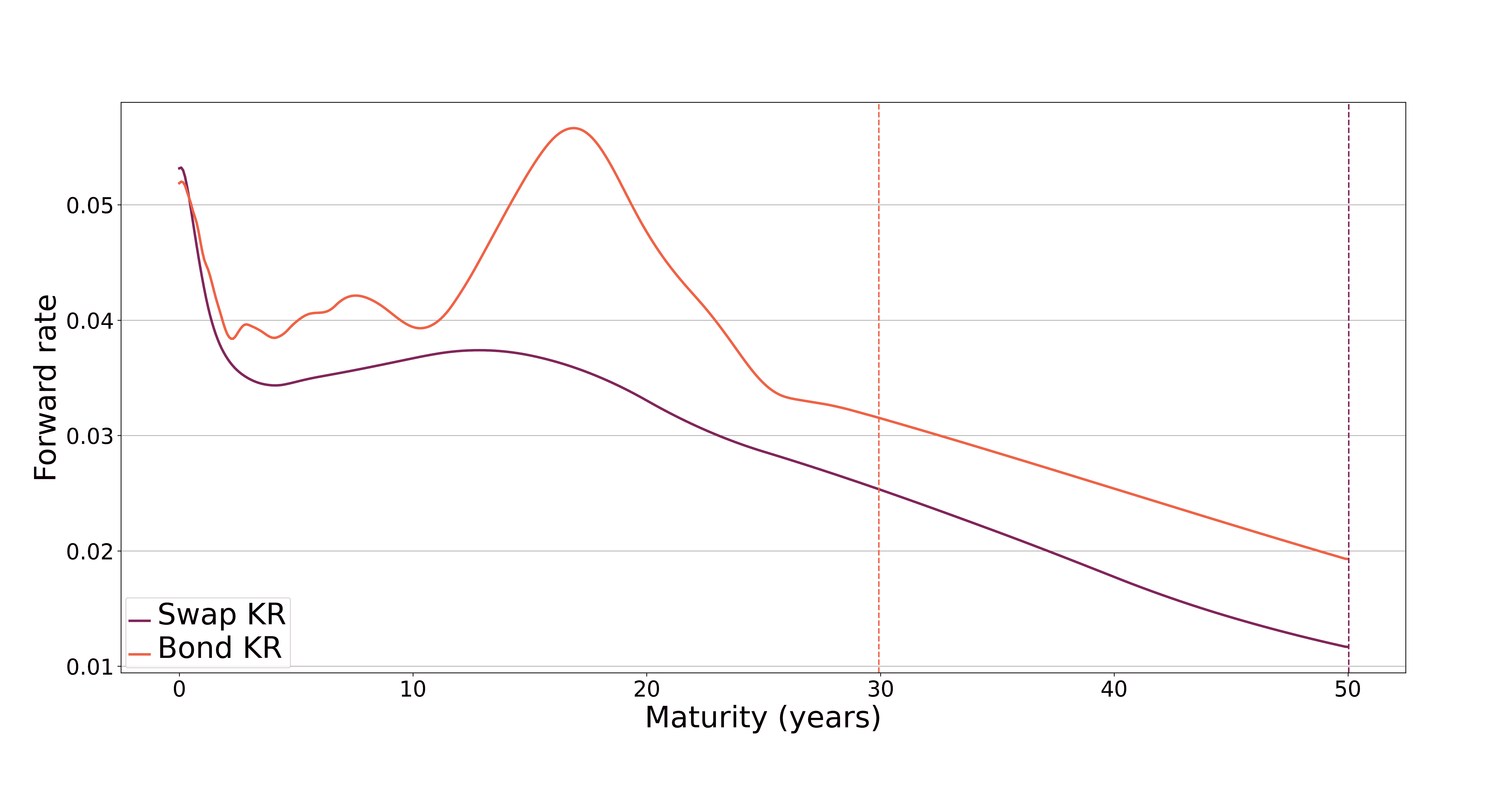
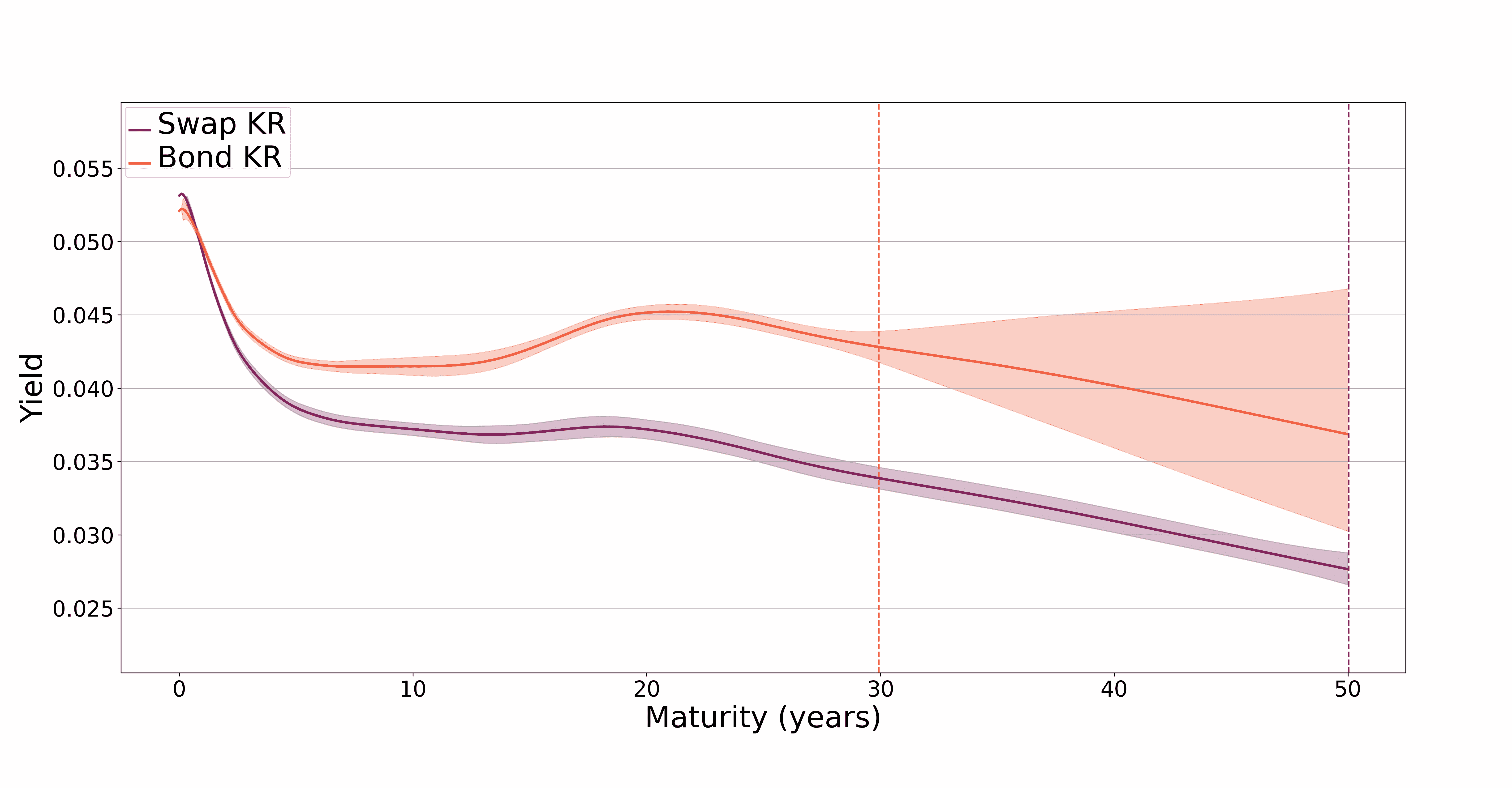
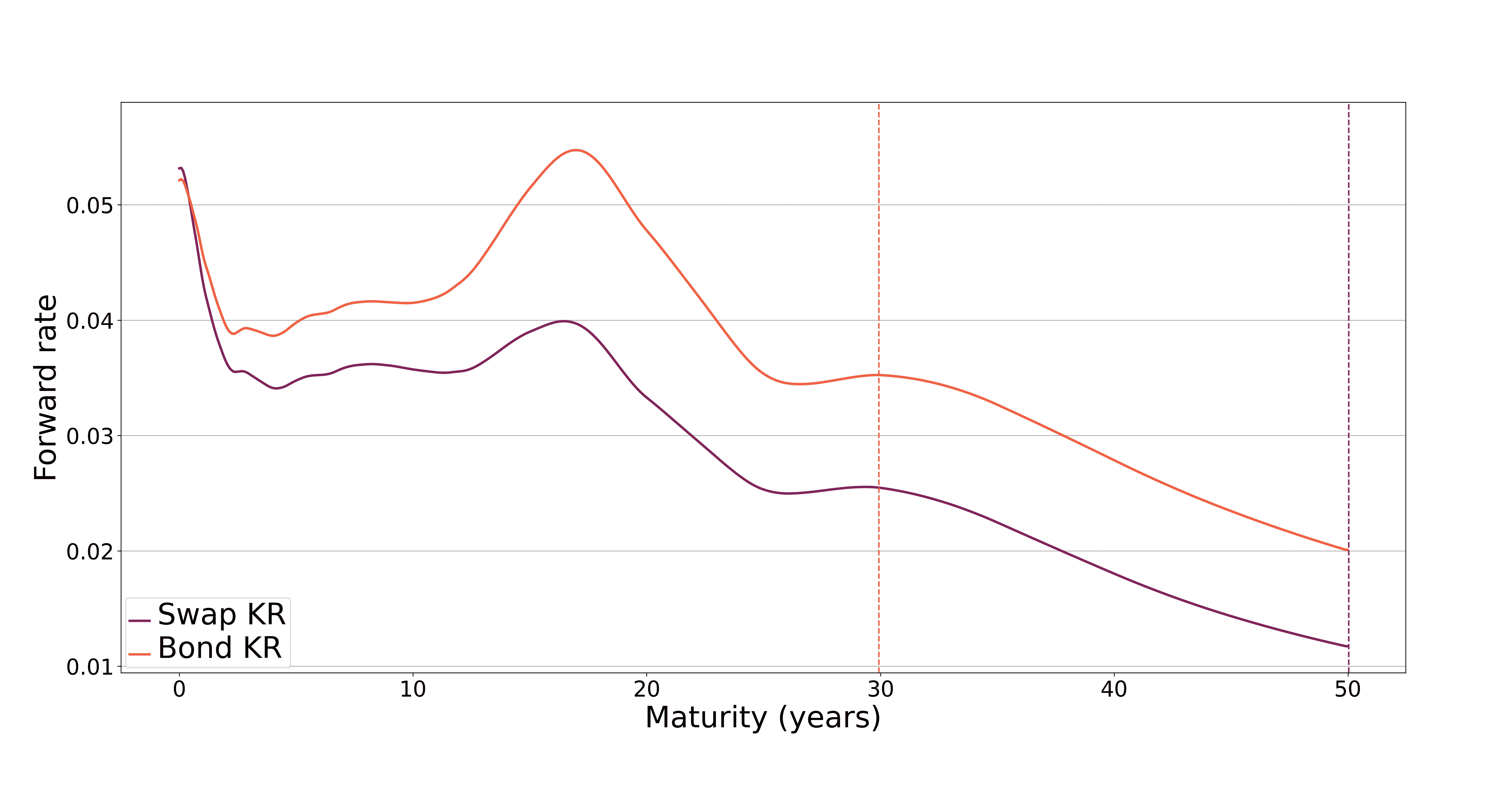
Figure 2 shows yield curves (left column) and forward curves (right column) for the EUR market on 2024-06-14, estimated under varying values of the transfer learning parameter .151515The yield curve consists of the annualized zero-coupon log returns, , and the forward curve is defined as the logarithmic derivative , for a scalar-valued discount curve . Shaded areas represent confidence bands derived from the Gaussian process view of the KR estimator, cut at for readability.161616Confidence bounds for the discount curve are computed as and , where . Confidence bands are not available for forward curves. German government bond maturities extend to 30 years, while ESTR swap tenors reach up to 60 years. Transfer learning leverages this longer maturity coverage to improve extrapolation for the bond yield curve. As increases, the confidence band for the bond yield curve narrows beyond 30 years, reflecting reduced uncertainty. In contrast, the swap yield curve, supported by denser data, remains largely unchanged. Within the interpolation range (up to 30 years), the bond yield curve is unaffected, confirming that transfer learning acts locally and preserves robustness in data-rich regions. As swaps typically span a broader maturity spectrum, information transfer tends to flow from swaps to bonds. The effects are even more apparent in the forward curves. For , the bond forward curve is visibly less smooth than the swap curve. For moderate values ( and ), the swap forward curve imparts a smoothing effect on the bond forward curve. However, for large values (), the direction of influence reverses, and the bond forward curve begins to distort the swap forward curve, illustrating the risk of excessive transfer.
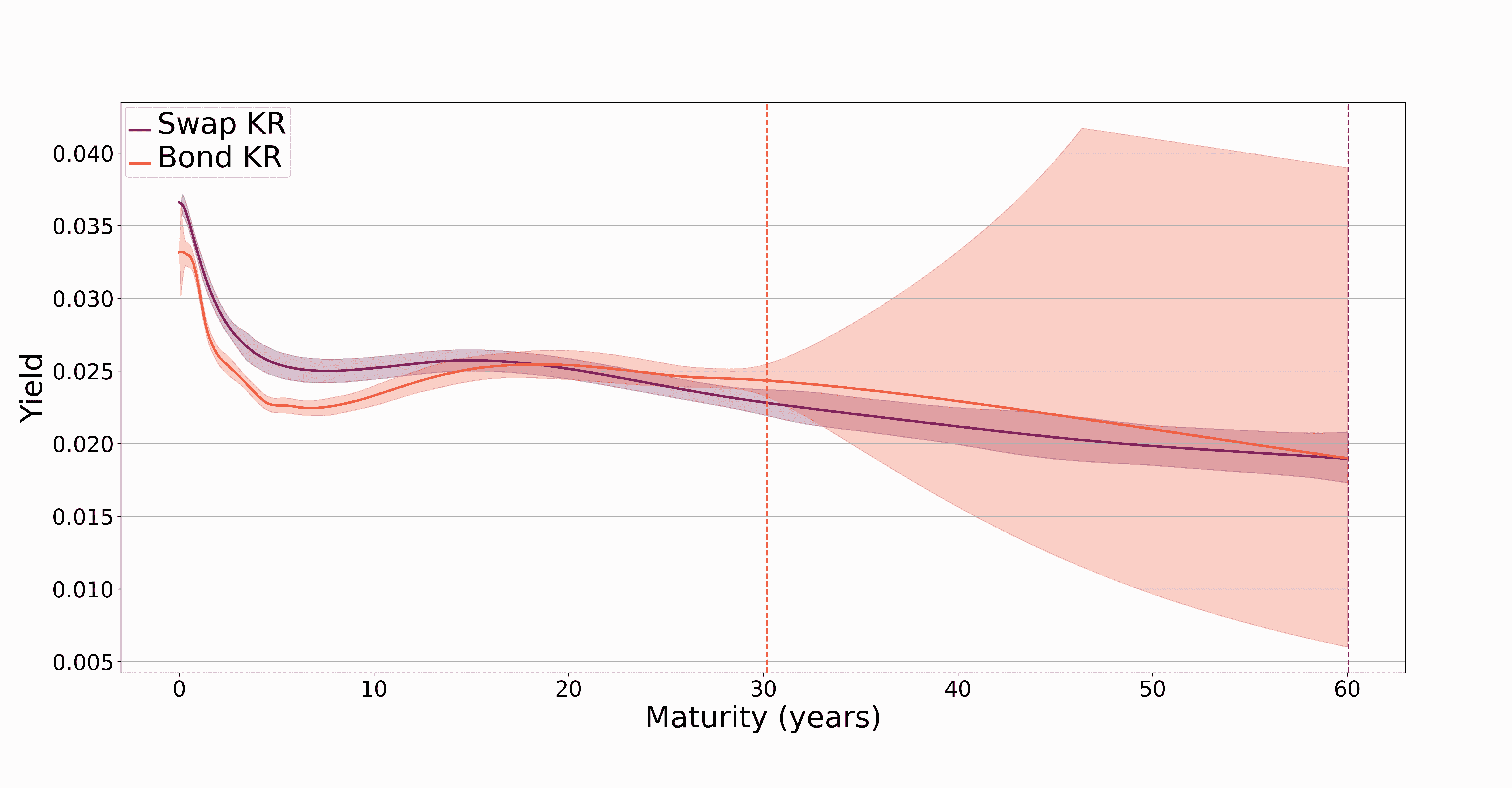
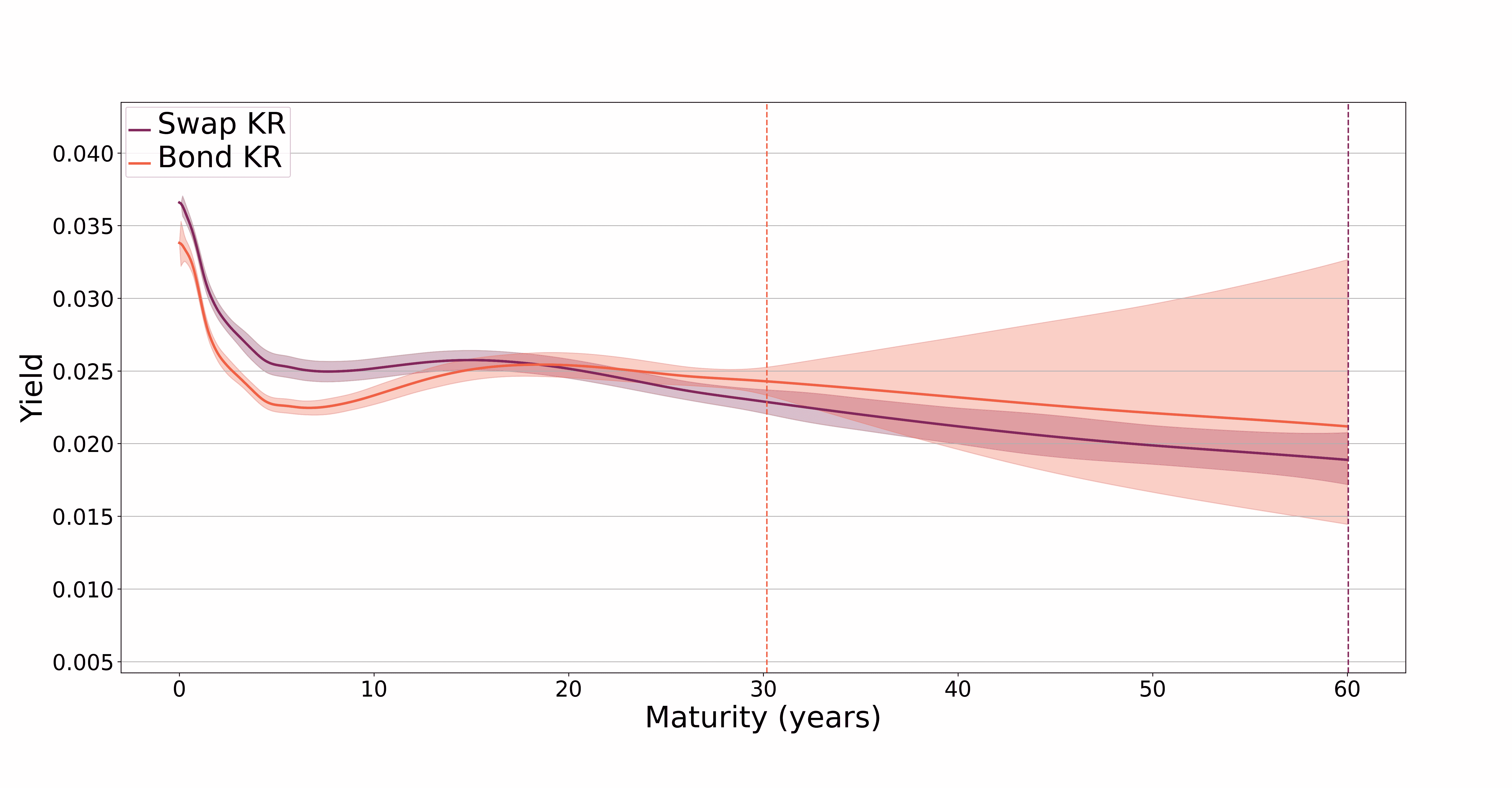
To quantify the transfer learning effects, Table 1 reports the change in yield at the longest available maturity for each currency at each date. Across all five reference dates, changes for the swap yield curve remain negligible (below 1 basis point), whereas the bond yield curve exhibits economically meaningful shifts ranging from to basis points.171717For context, [FPY24] and [CF24] report YTM root mean squared errors (RMSE) between 5 and 8 basis points.
| Date | ||||||
|---|---|---|---|---|---|---|
| Swap | Bond | Swap | Bond | Swap | Bond | |
| 2020-06-15 | 0.3 | -8.5 | 0.4 | -18.6 | 0.4 | -26.3 |
| 2021-06-15 | -0.1 | 1.8 | -0.3 | 0.6 | -0.3 | -3.5 |
| 2022-06-15 | 0.2 | 6.2 | 0.2 | 5.2 | 0.1 | -2.1 |
| 2023-06-15 | -0.4 | 8.6 | -0.7 | 1.0 | -0.9 | -8.5 |
| 2024-06-14 | -0.4 | 13.9 | -0.7 | 22.0 | -0.8 | 20.8 |
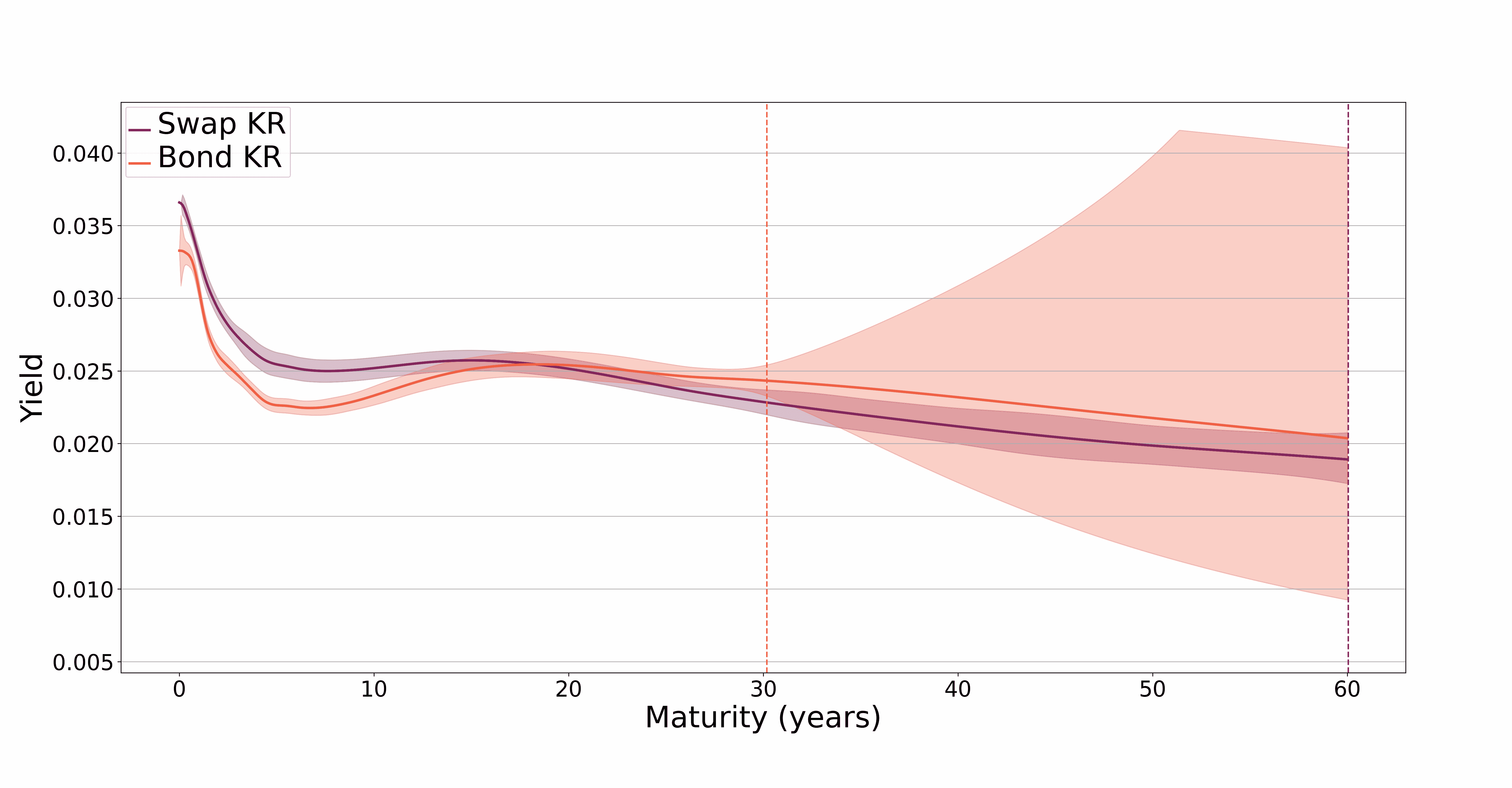
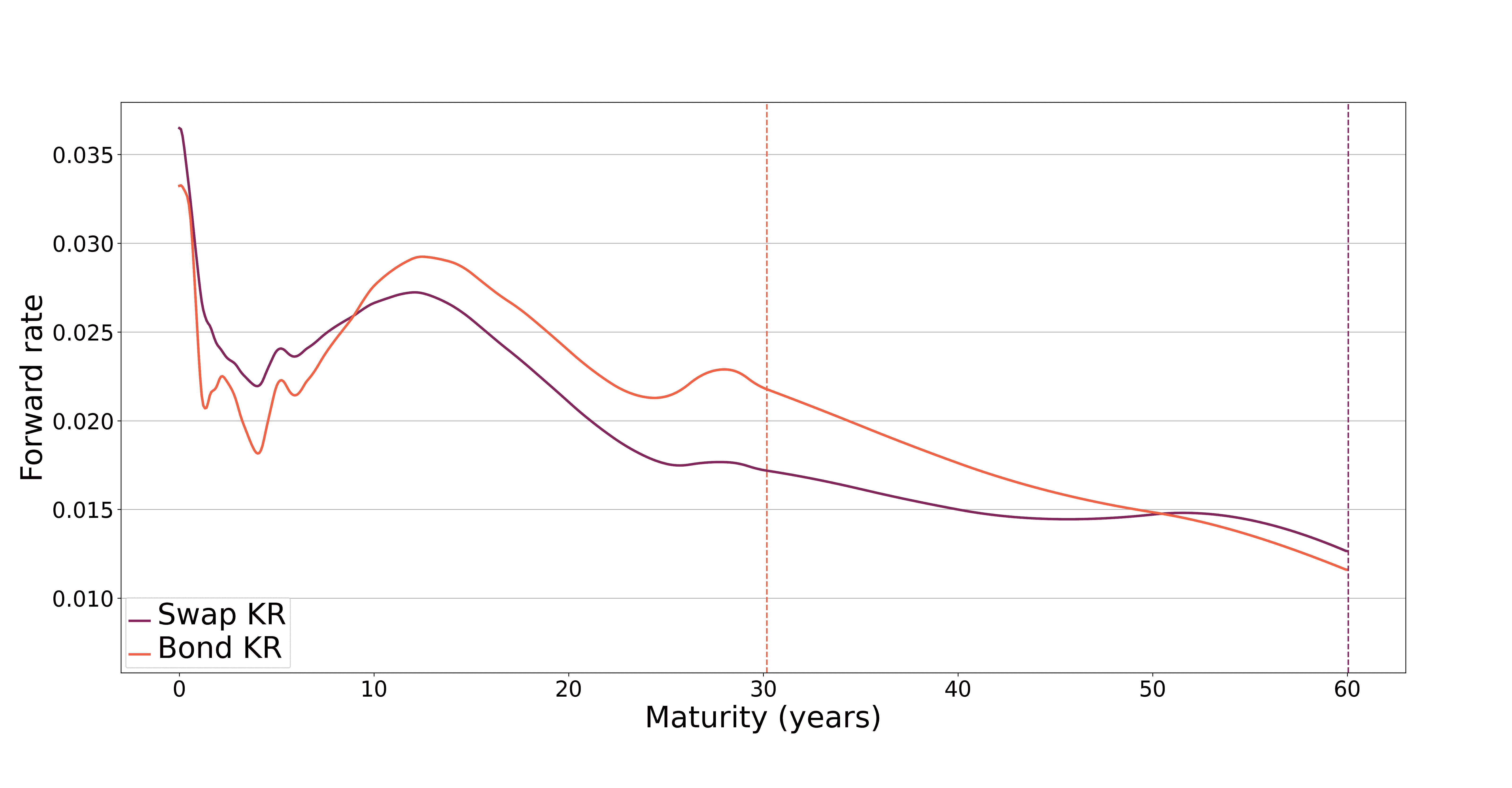
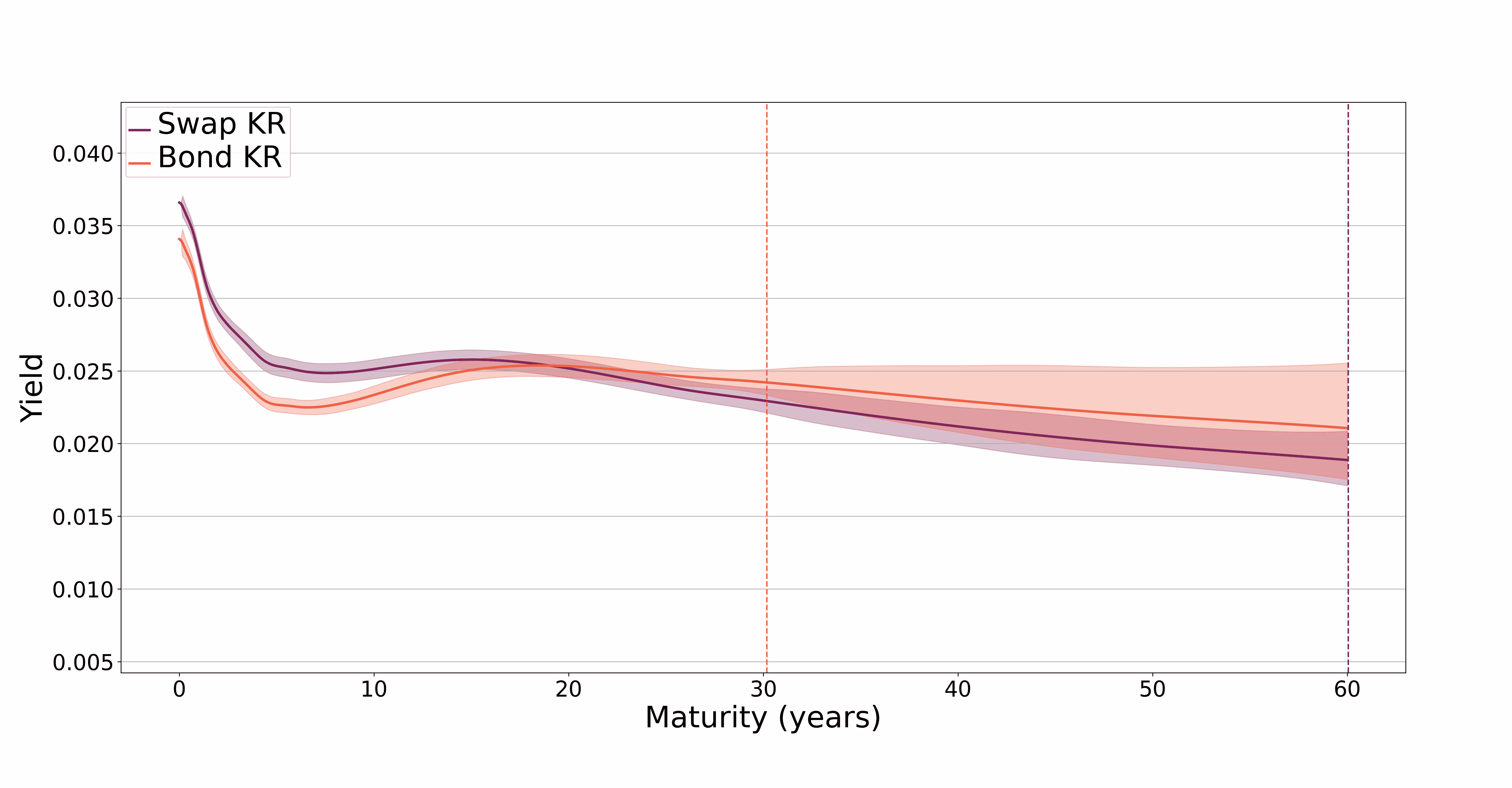
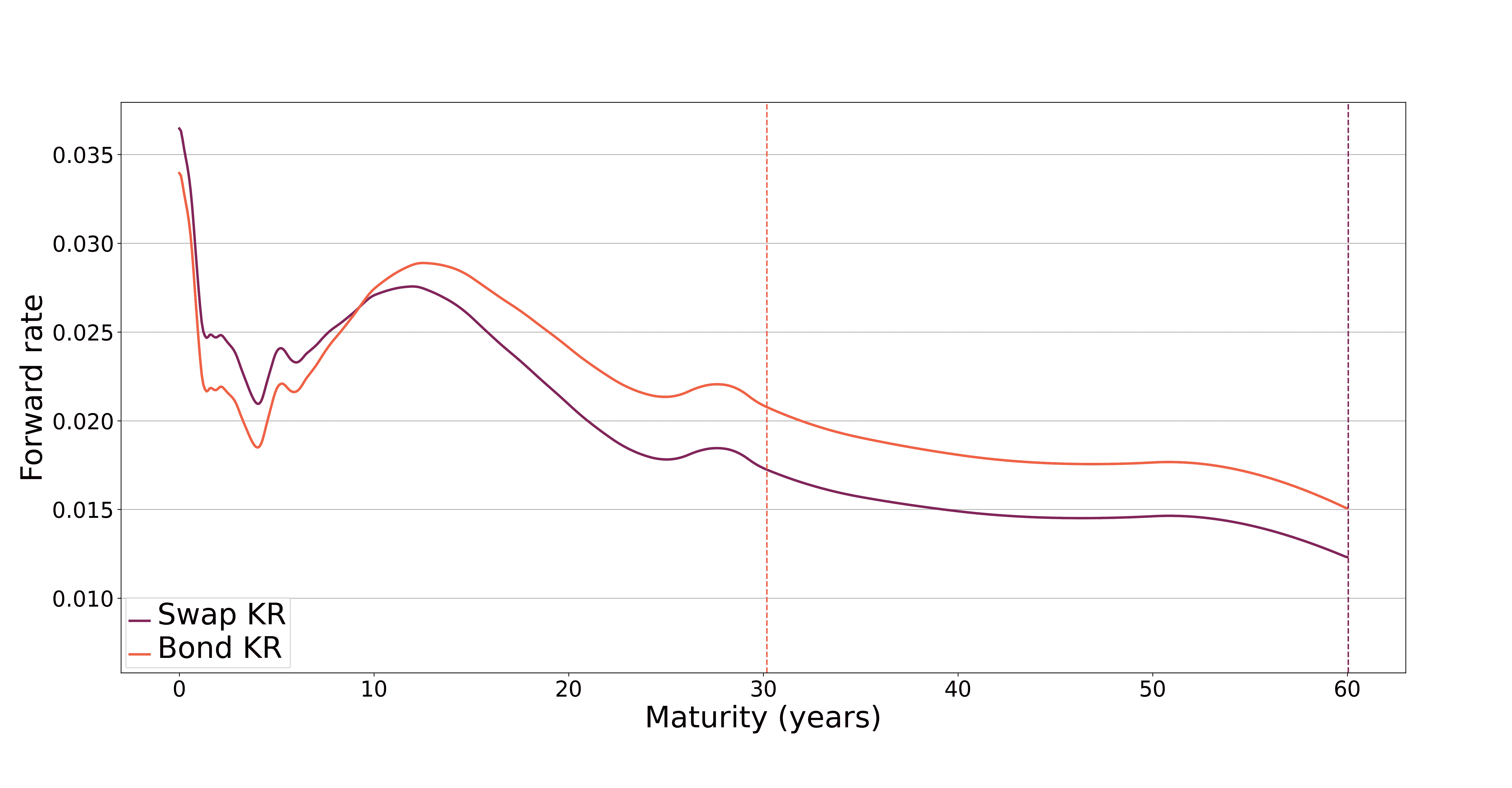
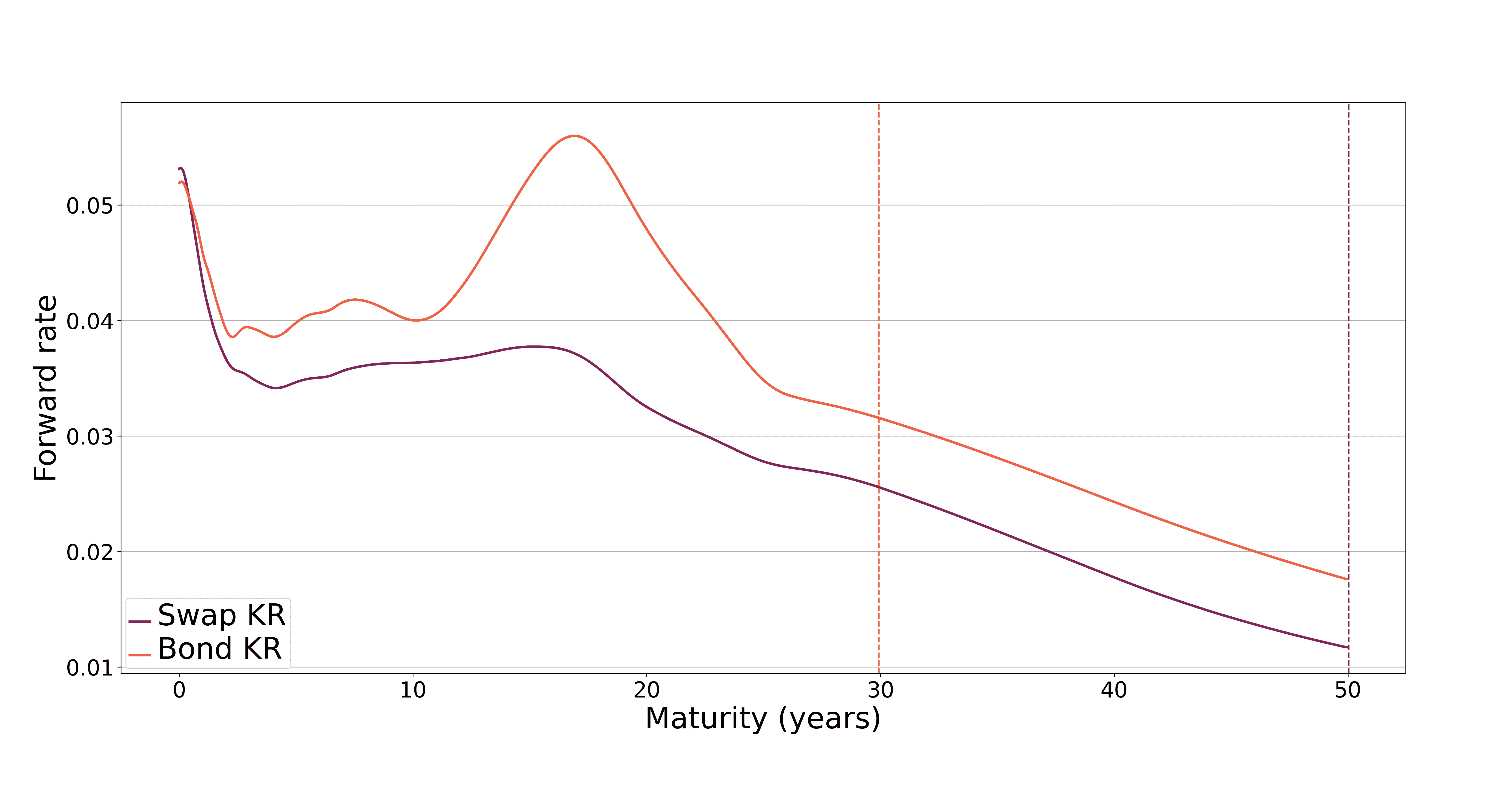
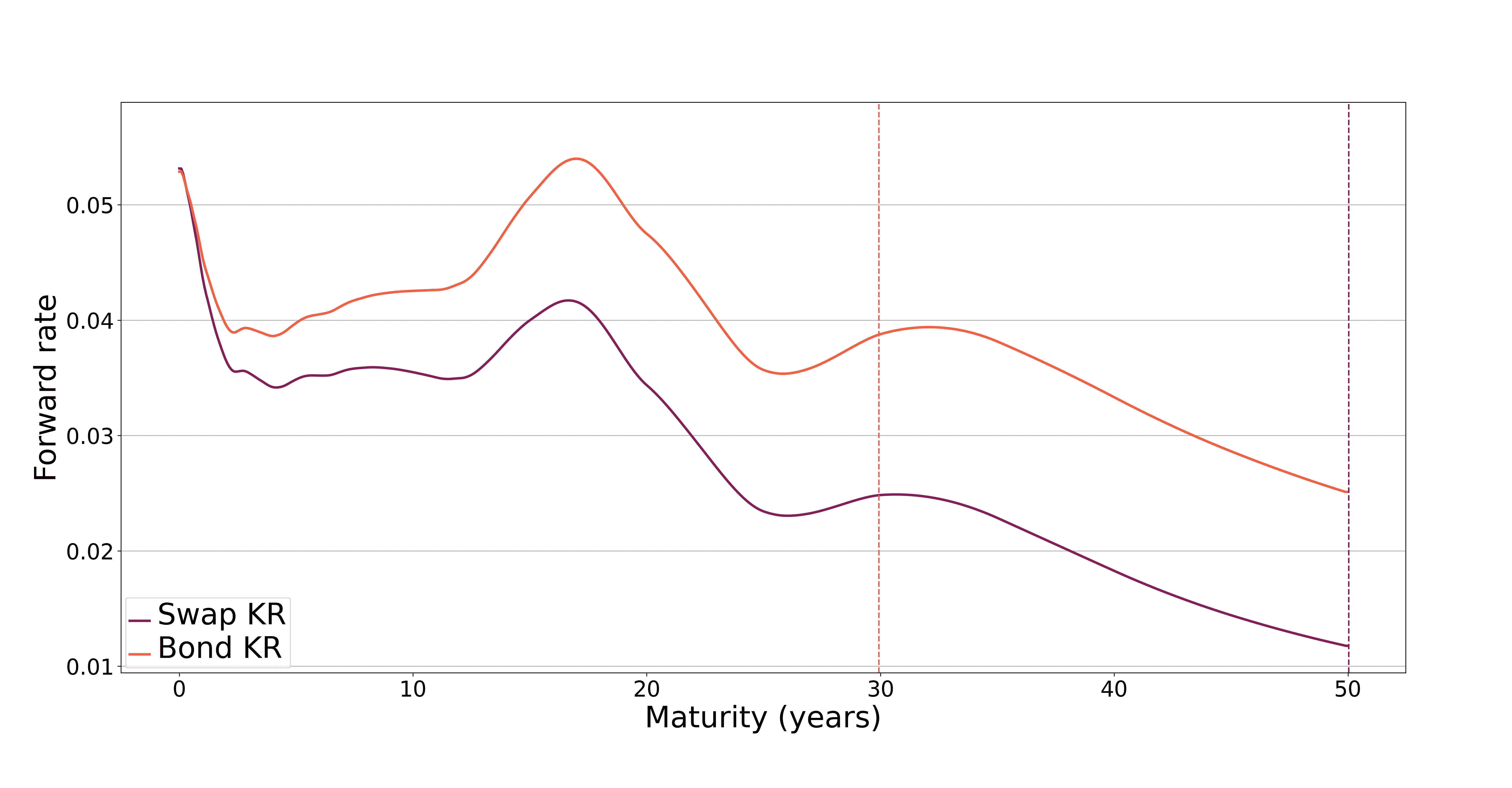
Figure 3 and Table 2 provide the corresponding results for the USD market on the same date. The patterns closely mirror those observed in the EUR case, reinforcing the conclusions above.
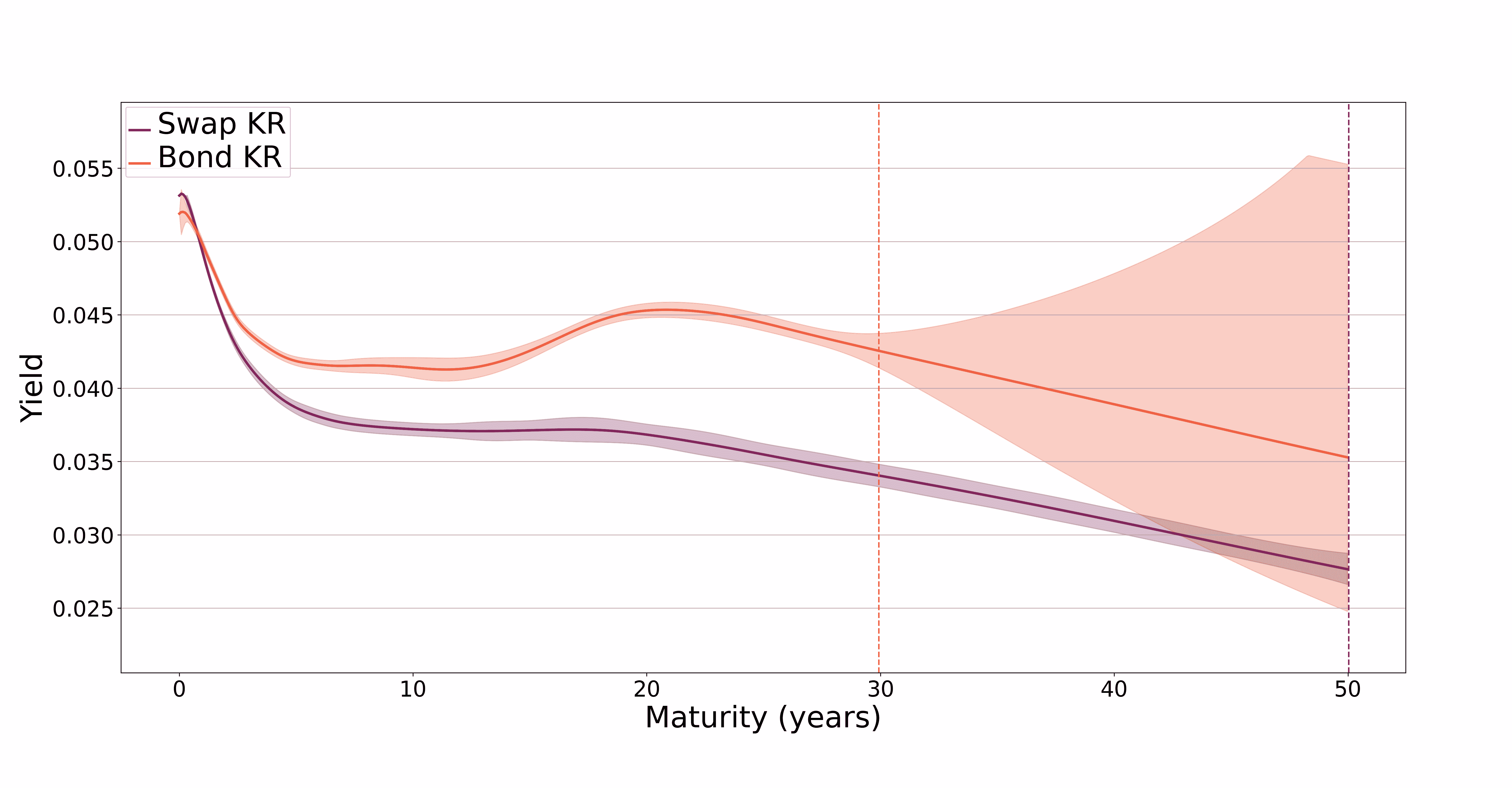
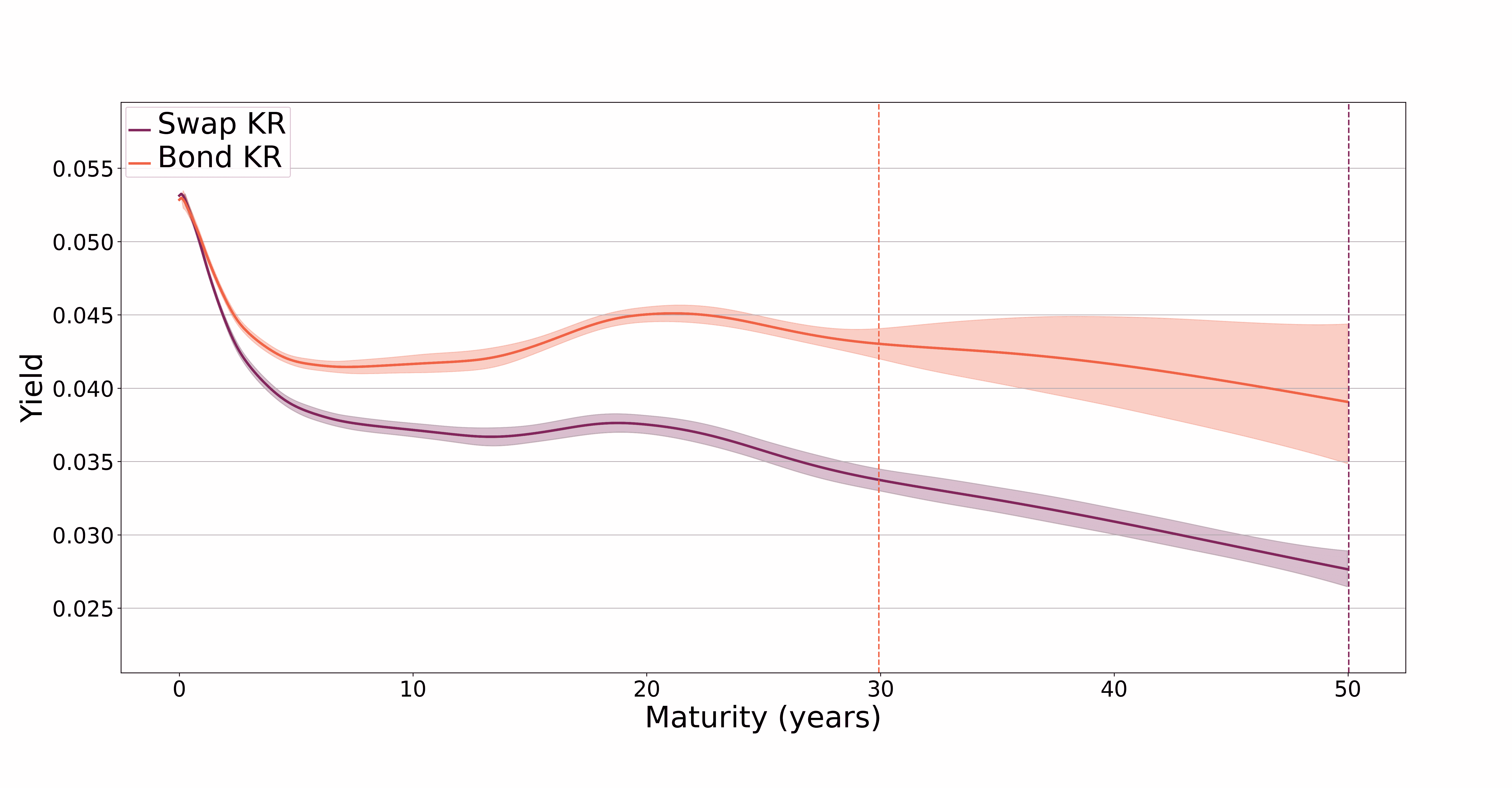
| Date | ||||||
|---|---|---|---|---|---|---|
| Swap | Bond | Swap | Bond | Swap | Bond | |
| 2020-06-15 | 0.1 | 4.8 | 0.1 | 12.3 | -0.3 | -2.5 |
| 2021-06-15 | -0.1 | 3.0 | -0.2 | 12.1 | -0.4 | 12.8 |
| 2022-06-15 | 0.3 | -4.8 | 0.6 | 13.3 | 0.4 | 25.2 |
| 2023-06-15 | 0.1 | -3.0 | 0.2 | 14.5 | 0.1 | 33.5 |
| 2024-06-14 | 0.1 | -3.8 | 0.1 | 12.0 | 0.0 | 34.0 |
These two examples are chosen for illustration due to their economic relevance and visual clarity. The full set of results, provided in the supplementary online appendix, consistently confirms the same qualitative pattern across all currencies and reference dates. In each case, transfer learning improves the estimation in data-scarce regions, particularly for government bond curves, while preserving robustness in well-identified segments.
7 Conclusion
We introduce a transfer learning framework for jointly estimating discount curves across fixed-income product classes. Building on the discounted cash flow principle, our approach extends kernel ridge regression to a vector-valued setting, resulting in a convex optimization problem with a closed-form solution in a vector-valued RKHS. A key feature is the use of separable operator-valued kernels, which enable regularization of curve spreads in an economically meaningful way.
We derive a norm decomposition for separable kernels, generalizing prior results and leading to a principled spread regularization term. The framework admits a Gaussian process interpretation, allowing uncertainty quantification in the vector-valued setting.
We show how standard fixed-income instruments, including coupon bonds, interest rate swaps, and cross-currency swaps, can be embedded in this structure. Empirical illustrations across CHF, EUR, GBP, and USD markets demonstrate that transfer learning improves extrapolation while leaving well-identified regions unaffected. A comprehensive empirical assessment is left for future work.
References
- [ARL12] Mauricio A. Alvarez, Lorenzo Rosasco, and Neil D. Lawrence. Kernels for vector-valued functions: A review. Foundations and Trends in Machine Learning, 4(3):195–266, 2012.
- [BHJ+19] Thomas Brophy, Niko Herrala, Raquel Jurado, Irene Katsalirou, Léa Le Quéau, Christian Lizarazo, and Seamus O’Donnell. Role of cross currency swap markets in funding and investment decisions. Occasional Paper Series 228, European Central Bank, August 2019.
- [Bjo09] Tomas Bjork. Arbitrage Theory in Continuous Time. Number 9780199574742 in OUP Catalogue. Oxford University Press, 2009.
- [BoEa] BoE. SONIA key features and policies. https://www.bankofengland.co.uk/markets/sonia-benchmark/sonia-key-features-and-policies (accessed: 08.05.2025).
- [BoEb] BoE. Sterling Overnight Index Average (SONIA). https://www.bankofengland.co.uk/markets/sonia-benchmark (accessed: 08.05.2025).
- [BRBV12] Luca Baldassarre, Lorenzo Rosasco, Annalisa Barla, and Alessandro Verri. Multi-output learning via spectral filtering. Machine Learning, 87, 2012.
- [Car97] Rich Caruana. Multitask learning. Machine Learning, 28(1):41–75, 1997.
- [CF24] Nicolas Camenzind and Damir Filipović. Stripping the swiss discount curve using kernel ridge regression. European Actuarial Journal, 14(2):371–410, June 2024.
- [Chr17] Chris Barnes, Clarus FT. Mechanics of cross currency swaps, 2017. https://www.clarusft.com/mechanics-of-cross-currency-swaps/ (accessed: 08.05.2025).
- [CWG19] Zexun Chen, Bo Wang, and Alexander N. Gorban. Multivariate gaussian and student-t process regression for multi-output prediction. Neural Computing and Applications, 32(8):3005–3028, dec 2019.
- [ECB] ECB. Euro short-term rate (€STR). https://www.ecb.europa.eu/stats/financial_markets_and_interest_rates/euro_short-term_rate/html/index.de.html (accessed: 08.05.2025).
- [FB87] Eugene F. Fama and Robert R. Bliss. The information in long-maturity forward rates. The American Economic Review, 77(4):680–692, 1987.
- [Fed] Fed. Secured Overnight Financing Rate (SOFR). https://www.newyorkfed.org/markets/reference-rates/sofr (accessed: 08.05.2025).
- [FLT17] Damir Filipović, Martin Larsson, and Anders B Trolle. Linear-rational term structure models. J. Finance, 72(2):655–704, April 2017.
- [FPY24] Damir Filipovic, Markus Pelger, and Ye Ye. Stripping the discount curve — a robust machine learning approach. Management Science, 2024. Accepted for publication.
- [GSW07] Refet S. Gürkaynak, Brian Sack, and Jonathan H. Wright. The U.S. treasury yield curve: 1961 to the present. Journal of Monetary Economics, 54(8):2291–2304, 2007.
- [HJ12] Roger A. Horn and Charles R. Johnson. Matrix Analysis. Cambridge University Press, 2 edition, 2012.
- [Int20] International Capital Market Association. A quick guide to the transition to risk-free rates in the international bond market, 2020. pdf (accessed: 08.05.2025).
- [JT95] Robert A Jarrow and Stuart M Turnbull. Pricing derivatives on financial securities subject to credit risk. J. Finance, 50(1):53, March 1995.
- [Kat95] Tosio Kato. Perturbation theory for linear operators. Classics in Mathematics. Springer-Verlag, Berlin, 1995. Reprint of the 1980 edition.
- [KDP+16] Hachem Kadri, Emmanuel Duflos, Philippe Preux, Stéphane Canu, Alain Rakotomamonjy, and Julien Audiffren. Operator-valued kernels for learning from functional response data. Journal of Machine Learning Research, 17(20):1–54, 2016.
- [LW21] Yan Liu and Jing Cynthia Wu. Reconstructing the yield curve. Journal of Financial Economics, 142(3):1395–1425, 2021.
- [MM] Andréa M. Maechler and Thomas Moser. Life after Libor: A new era of reference interest rates. https://www.snb.ch/en/publications/communication/speeches/2022/ref_20220331_amrtmo (accessed: 08.05.2025).
- [MP04] Charles A. Micchelli and Massimiliano Pontil. Kernels for multi-task learning. NIPS, 2004.
- [MP05] Charles A. Micchelli and Massimiliano Pontil. On learning vector-valued functions. Neural Computation, 17, 2005.
- [NS87] Charles R. Nelson and Andrew F. Siegel. Parsimonious modeling of yield curves. The Journal of Business, 60(4):473, January 1987.
- [PR16] Vern I. Paulsen and Mrinal Raghupathi. An introduction to the theory of reproducing kernel Hilbert spaces, volume 152 of Cambridge Studies in Advanced Mathematics. Cambridge University Press, Cambridge, 2016.
- [PY10] Sinno Jialin Pan and Qiang Yang. A survey on transfer learning. IEEE Trans. Knowl. Data Eng., 22(10):1345–1359, October 2010.
- [Ran23] Angelo Ranaldo. Foreign exchange swaps and cross-currency swaps. In Refet S. Gürkaynak and Jonathan H. Wright, editors, Research Handbook of Financial Markets, Chapters, chapter 20, pages 451–469. Edward Elgar Publishing, 2023.
- [RW05] Carl Edward Rasmussen and Christopher K I Williams. Gaussian processes for machine learning. Adaptive Computation and Machine Learning series. MIT Press, London, England, November 2005.
- [She08] Daniel Sheldon. Graphical multi-task learning. Technical report, Cornell University, 2008.
- [SIX] SIX. Swiss Reference Rates (SARON). https://www.six-group.com/en/market-data/indices/switzerland/saron.html (accessed: 08.05.2025).
- [SK03] Alexander J. Smola and Risi Kondor. Kernels and Regularization on Graphs, page 144–158. Springer Berlin Heidelberg, 2003.
- [SS19] Andreas Schrimpf and Vladyslav Sushko. Beyond libor: a primer on the new benchmark rates. BIS Quarterly Review, 2019.
- [Sve94] Lars Svensson. Estimating and interpreting forward interest rates: Sweden 1992 - 1994. NBER Working Papers 4871, National Bureau of Economic Research, Inc, 1994.
- [SW01] Andrew Smith and Tim Wilson. Fitting yield curves with long term constraints. Working paper, 2001.
- [Tea21] Risk.net Editorial Team. Beyond libor: the impact of sofr on rates, bonds and loans, 2021. https://www.risk.net/insight/markets/7957455/beyond-libor-the-impact-of-sofr-on-rates-bonds-and-loans (accessed: 08.05.2025).
- [Wik] Wikipedia contributors. Kernel methods for vector output. https://en.wikipedia.org/wiki/Kernel_methods_for_vector_output (accessed: 08.05.2025).
- [WJ24] David Wu and Robert A. Jarrow. The Treasury–SOFR swap spread puzzle explained, 2024. Available at SSRN: https://ssrn.com/abstract=4904777.
- [WKW16] Karl Weiss, Taghi M Khoshgoftaar, and Dingding Wang. A survey of transfer learning. J. Big Data, 3(1), December 2016.
Appendix A Vector-valued reproducing kernel Hilbert spaces
This appendix presents the theoretical background on vector-valued RKHS that underpins our transfer learning framework. For completeness, we begin by recalling the definition and main properties of vector-valued RKHS, following [PR16, Chapter 6]. Let be any set and .
Definition A.1.
An -valued RKHS on is a Hilbert space consisting of functions such that for every , the linear evaluation map given by is bounded.
An -valued RKHS has a reproducing kernel function defined by , where we identify a linear operator on with its -matrix representation in the standard Euclidean basis of . denotes the adjoint operator. We immediately obtain that and , for any , , . Moreover, we see that is symmetric in the following sense,
| (16) |
Note, however, that the matrices are not symmetric for in general.181818Many papers in the literature assume that the matrices are symmetric. But this is not the case in general, and, in fact, it excludes many examples. Moreover, for any finite points the operator on is positive semi-definite in the sense that for all choices of vectors we have
| (17) |
Conversely, this leads to the following definition.191919Note that [PR16, Definition 6.11] does not require (16) because they work on complex Hilbert spaces, where the non-negativity, that is, (17) with replaced by its complex conjugate, already implies that .
It follows by inspection that a function is a -valued kernel function if and only if there exists a scalar kernel function on such that .
Example A.3.
The concept of matrix-valued kernels is surprisingly strong as it is somewhat difficult to generate examples easily. However, one possible way is to let be scalar kernels on , then is a -valued kernel. Indeed, property (16) holds because is symmetric. Property (17) is valid since
where the inner sums are non-negative due to the kernel property of each scalar kernel .
Moore’s vector-valued theorem [PR16, Theorem 6.12] states that for every -valued kernel function there exists a unique -valued RKHS such that is its reproducing kernel function. Moreover, functions of the form
| (18) |
are dense in , see [PR16, Proposition 6.7].202020Note that (18) differs from the corresponding formulas in [ARL12, page 209] and the wikipedia page [Wik]. The latter formulas are correct only if is a symmetric matrix, which in view of (16) is not true in general. A special class of -valued kernels are separable kernels. In fact, as it turns out they are tractable and easy to interpret.
Definition A.4.
A -valued kernel on is separable if it can be written as for some -matrix and a scalar kernel on . In view of (16), the matrix is necessarily symmetric positive semi-definite.
Remark A.5.
Separable kernels are one of the simplest matrix-valued kernel. If we regard kernels as similarity measures, encodes similarity across components while encodes similarity across the space .
The following theorem provides an important representation result, which is at the heart of transfer learning in this paper.
Theorem A.6.
Let be the vector-valued RKHS corresponding to the separable kernel . Let denote the RKHS corresponding to the scalar kernel . Let be any generalized inverse -matrix of such that . Then the following hold.
-
(i)
is isomorphic to the direct sum , where .
-
(ii)
as sets, with equality if and only if is non-singular.
-
(iii)
For any , the -norm can be expressed as
(19) - (iv)
Proof.
We define the linear subspace of that consists of all functions of the form
| (21) |
From (18) we know that is dense in . Similarly, we define the dense subspace of of all functions of the form , for . Consequently, the direct sum is a dense subspace of .
We prove the theorem in two steps. First, we prove all statements for and replaced by and . Second, we argue by the continuous extension principle that all results carry over to and .
We let denote the reduced spectral decomposition where is an orthogonal -matrix such that , and contains the positive eigenvalues of .
We define the linear operator , by . The operator is injective, because implies that and thus for all , hence . Here we assume that is minimal in the sense that are linearly independent in , without loss of generality. We claim that is also surjective, . Indeed, any can be written as , for some , , . Define the linear operator by . As the -matrix has full rank , there exist such that . Then given by is a pre-image of , because . We conclude that is a linear bijection with inverse given by , which proves (i).
We also obtain that the components of any are linear combinations of functions and thus elements in themselves. As if and only if is non-singular, this proves (ii).
Next we claim that (19) holds for . Indeed, on one hand we have
by the basic reproducing kernel property of . On the other hand, the right hand side of (19) equals
which equals the former and thus proves (iii).
We now extend the validity of the above proved properties to and . Thereto, when writing for , we observe that the right hand side of (19) becomes
| (22) |
Indeed, implies , and thus for any , which shows (22).212121In more detail: we have , and hence , which equals the right hand side of (22). We obtain the bounds
We infer that is bounded with operator norm . In the same vein, is bounded with operator norm . By the extension principle for bounded densely defined operators on Banach spaces, [Kat95, Section III.2.2], uniquely extends to an invertible bounded operator with inverse given by the respective extension of . As norm convergence in and implies point-wise convergence, we have and , for all and . The validity of (i), (ii), (iii), (iv) for and now follows by continuity arguments. ∎
Remark A.7.
The following two auxiliary lemmas are of independent interest and potentially useful for the specification of a matrix-valued kernel. They provide general elementary decomposition results, which are known as kernel normalization in the scalar case.
Lemma A.8.
Any -valued kernel can be decomposed in the following way
| (23) |
where is a normalized -valued kernel such that , and is a diagonal matrix with non-negative elements, for all and .
A particular decomposition is given by
| (24) |
and
| (25) |
and we set
| (26) |
On the other hand, any such decomposition necessarily satisfies (24) and (25).222222Property (26) does not necessarily hold. Indeed, consider the finite set and and suppose that and . Then , and is a normalized kernel satisfying the decomposition (23), but not (26).
Proof.
In the special case of separable kernels, Lemma A.8 extends as follows.
Lemma A.9.
Let be a separable kernel. Then the normalized kernel given by (25) and (26) is separable of the form for the symmetric positive semi-definite matrix given by
and we set otherwise and the scalar kernel given by
and we set otherwise. In particular, and are normalized in the sense that and , for all and .
Proof.
It is enough to show that is a symmetric positive semi-definite matrix and a scalar kernel. This can both be proved using similar arguments as in the proof of Lemma A.8. ∎
Appendix B Proofs
This appendix provides the proofs of the results stated in the main text, based on the foundational material presented in Appendix A.
B.1 Proof of Theorem 2.1
Let be the sampling operator as in equation (27). For any define such that is the -th row of , and is the -th component of , and the corresponding weight. Then the weighted mean-squared pricing error can be written as
Similarly for the constraints, where .
It then follows that the solution of the KR problem must lie in the orthogonal complement of the null space of . That is, , for some . The rest of the proof now follows as in the scalar case [FPY24, Theorem A.1], using Lemma B.1 below. This completes the proof of Theorem 2.1.
Lemma B.1.
Define the sampling operator by
| (27) |
The adjoint is given by
| (28) |
where is the -th row of the matrix with . Moreover, is the matrix representation of the linear operator in the standard Euclidean basis of .
B.2 Proof of Theorem 4.1
According to Theorem A.6(iv) it is enough to construct a symmetric positive definite matrix such that and for . Therefore, we parameterize by the spread smoothness parameters , as defined in (10).
By construction, the matrix is strictly diagonally dominant, , for all , and hence positive definite, see [HJ12, Theorem 6.1.10]. Hence is symmetric and positive definite leading to a valid separable kernel. Theorem A.6 implies that the norm of the vector-valued RKHS with separable kernel is given by (9). Theorem A.6 also implies that the optimization problem (8) over the product space is equivalent to the KR problem (4) with norm (9) for .
Remark B.2.
The matrix in (10) is strictly diagonally dominant, by construction. This is sufficient for being positive definite. However, not every symmetric positive definite matrix is strictly diagonally dominant. An example is given by
for any . Indeed, the characteristic polynomial is . Hence the eigenvalues of are positive, , and is positive definite. However, is not diagonally dominant, as . In that sense, specification (9) is a special case of a vector-valued RKHS with separable kernel as discussed in Theorem A.6
B.3 Proof of Lemma 6.1
Under the assumption of the lemma, we have after multiplication with
where we write . Therefore , which proves the claim.
Appendix C Arbitrage-free pricing framework
In this appendix, we place the discounted cash flow equation (1) within an arbitrage-free pricing framework, following standard principles of asset pricing theory (see, e.g., [Bjo09]).
Let be a probability space equipped with a filtration representing the flow of market information. All processes are assumed to be adapted to this filtration. The pricing measure is risk-neutral with respect to a numeraire , interpreted as the money market account, satisfying and accruing at the overnight RFR. The present value at time of an -measurable cash flow paid at time is
| (29) |
where is the price of a risk-free discount bond maturing at , and denotes the -forward measure defined via the Radon–Nikodym derivative .
C.1 Non-defaultable bonds
Bonds issued by highly rated sovereigns, such as U.S. Treasuries or German government bonds, are typically regarded as non-defaultable (or risk-free). The discounted cash flow equation (1) applies directly with for such a bond paying nominal coupons at dates and the notional of one at the maturity .
C.2 Defaultable bonds
Defaultable (or credit-risky) bonds include corporate debt and sovereign debt issued by less creditworthy countries. These instruments generally trade at a spread over the risk-free curve to reflect credit risk. Let denote the default time (which is a stopping time). Under the widely used recovery-of-treasury assumption (see [JT95]), the cash flow at is modeled as
where is a deterministic recovery rate. Applying (29), we obtain
which motivates the effective discount factor
| (30) |
Defaultable bonds are typically grouped by credit rating. Assuming all bonds within a given rating class share the same default distribution and recovery profile, the class admits a common discount curve , and the discounted cash flow equation (1) applies.
C.3 RFR-based swaps
An RFR-based swap is an interest rate swap whose floating leg is linked to the money market account , which accrues at the RFR, such as SOFR in the United States or SARON in Switzerland, see [Fed, SIX]. Under the no-arbitrage assumption, RFR-based swap contracts should be priced using the same discount curve as creditworthy government bonds denominated in the same currency. In practice, however, a swap–government bond spread is observed. This spread arises due to market frictions and regulatory effects, and lies outside the scope of our simple arbitrage-free pricing framework, see, e.g., [WJ24].
As for the fixed leg, let denote the payment dates, with notional normalized to one. For a given annualized swap rate , the fixed cash flow at time is with . By (29), the present value of the fixed leg is
Let denote the reset and payment dates of the RFR floating leg, again with notional normalized to one. The floating cash flow at time corresponds to the simple return of the money market account over the accrual period , given by . Using (29) and observing the telescoping structure of the discounted cash flows, we obtain , from which the present value of the RFR floating leg follows as
| (31) |
Although the above specification, where floating cash flows are ”fixed in arrears,” has become the standard, see, e.g., [Int20, Tea21], an alternative is to define the floating rate over as the simple return on a discount bond, . Here, with a slight abuse of notation, we denote by the time- value of a risk-free discount bond maturing at , such that . Under this alternative specification, the present value of the floating leg remains given by (31), which follows directly as a simple consequence of the arbitrage-free pricing formula (29).
C.4 IBOR swaps
Interest rate swaps whose floating leg is tied to an interbank loan term rate (IBOR) reflect credit and liquidity risk, which we model by adding a spread to the floating cash flows. For example, EURIBOR can be viewed as the sum of the risk-free ESTR and a credit spread capturing interbank risk.232323Strictly speaking, ESTR is not secured, unlike SOFR. However, as an overnight rate, its credit risk is considered negligible, and we treat it as risk-free for our purposes.
Formally, using the same tenor structures for the floating and fixed legs as in Subsection C.3, the floating cash flow of an IBOR swap at time is given by , where denotes a spread that reflects the credit and liquidity risk of lending in the interbank market over the period . The present value of the IBOR swap’s floating leg is then
| (32) |
As in the case of defaultable bonds discussed in Subsection C.2, we classify IBOR swaps according to the length of the accrual period (tenor) of the floating leg, such as quarterly, semiannual, or annual. We assume that all IBOR swaps within a given tenor class share the same spread structure, which gives rise to a common discount curve . This curve is determined from the discounted cash flow equation (1), in conjunction with the expressions for the floating and fixed cash flows, resulting from (11) and (12), respectively.
C.5 Cross-currency swaps
We are considering a standard floating–floating XCCY swap. The tenor structure of the cash flows is given by . The XCCY consists of two legs, leg and leg . Leg is treated as the liquid leg. Thus, the basis spread is added to leg which has a normalized notional of . The initial notional of leg is set to the spot exchange rate, . The MTM feature is sometimes applied to leg .
We now show that, when present, the MTM adjustments do not affect the present value of leg . According to Clarus Financial Technology,242424Clarus FT is a data and analytics provider focused on OTC derivatives markets. See [Chr17] for a discussion of MTM mechanics in cross-currency swaps. the floating cash flow at each payment date consists of the simple return on the money market account applied to the MTM notional over the accrual period , minus the change in MTM notionals over that period, and plus the MTM notional at maturity if . Formally, this gives
where denotes the MTM notional in currency at time , and is the corresponding money market account.
Discounting each cash flow by the money market account and simplifying the telescoping sum yields
which is known (deterministic) at time and equal to the initial notional. Hence, the present value of leg is given by , as in the case without MTM. This demonstrates that MTM adjustments, while relevant for risk management, do not affect the arbitrage-free valuation of the liquid leg.