Simple Semi-supervised Knowledge Distillation from Vision-Language Models via Dual-Head Optimization

Abstract

Vision-language models (VLMs) have achieved remarkable success across diverse tasks by leveraging rich textual information with minimal labeled data. However, deploying such large models remains challenging, particularly in resource-constrained environments. Knowledge distillation (KD) offers a well-established solution to this problem; however, recent KD approaches from VLMs often involve multi-stage training or additional tuning, increasing computational overhead and optimization complexity. In this paper, we propose Dual-Head Optimization (DHO)—a simple yet effective KD framework that transfers knowledge from VLMs to compact, task-specific models in semi-supervised settings. Specifically, we introduce dual prediction heads that independently learn from labeled data and teacher predictions, and propose to linearly combine their outputs during inference. We observe that DHO mitigates gradient conflicts between supervised and distillation signals, enabling more effective feature learning than single-head KD baselines. As a result, extensive experiments show that DHO consistently outperforms baselines across multiple domains and fine-grained datasets. Notably, on ImageNet, it achieves state-of-the-art performance, improving accuracy by 3% and 0.1% with 1% and 10% labeled data, respectively, while using fewer parameters.

1 Introduction

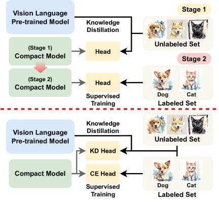
Figure 1: (Top): Previous multi-stage VLMs distillation methods. (Bottom): Our single-stage distillation framework with DHO.

Vision-Language Models (VLMs), which learn joint vision-language representations through contrastive learning (Radford et al., 2021; Jia et al., 2021), have shown promising results in few-shot scenarios by leveraging rich textual information from pre-training. Recent work has explored various adaptation strategies for VLMs with limited labeled data, including parameter-efficient approaches such as linear probing (Radford et al., 2021; Li et al., 2022; Huang et al., 2024), lightweight adapters (Gao et al., 2024; Zhang et al., 2021; Yu et al., 2023b; Silva-Rodriguez et al., 2024), and prompt-based fine-tuning methods (Jia et al., 2022; Zhou et al., 2022b, a; Khattak et al., 2023a; Zhu et al., 2023; Khattak et al., 2023b; Zhao et al., 2024; Roy and Etemad, 2023; Zhang et al., 2024a; Lafon et al., 2025), demonstrating the potential of VLMs for data-limited visual recognition tasks.

However, the substantial computational requirements and large model sizes of foundation models often make them impractical for deployment in resource-constrained environments, such as mobile devices Sandler et al. (2018). While compact models could address these challenges, they typically struggle with limited performance, especially with limited labeled data. Semi-supervised learning techniques Sohn et al. (2020); Assran et al. (2021); Cai et al. (2022); Zheng et al. (2023) leveraging unlabeled data can help address these performance limitations, but they are often suboptimal for small models compared to the performance of foundation models, such as VLMs.

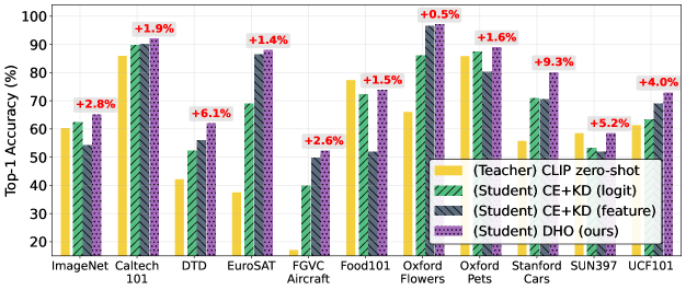
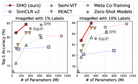
Figure 2: (Left): DHO consistently outperforms single-head baselines on 11 datasets under 16-shot semi-supervised setting. The improvements are evaluated in comparison to the second-best one. (Right): DHO achieves new SoTA on ImageNet in both 1% and 10% labeled data setting, with fewer parameters.

Knowledge distillation (KD) Hinton (2015) has emerged as a promising approach for transferring capabilities from large VLMs to more compact models. However, existing methods primarily focus on distilling large VLMs into smaller ones through general-purpose training Fang et al. (2021b); Sun et al. (2023b); Wu et al. (2023); Yang et al. (2024a); Vasu et al. (2024); Udandarao et al. (2024); Yang et al. (2024c) or preceding with unsupervised distillation stage Vemulapalli et al. (2024); Wu et al. (2025), which often requires additional fine-tuning for specific target tasks (Figure˜1-(Top)). This multi-stage pipeline not only incurs extra computational overhead but also limits the direct transfer of the teacher model’s zero- and few-shot capabilities to the student model for task-specific applications, suggesting a need for more efficient distillation methods that can preserve the teacher’s expertise for the intended task.

In contrast, conventional KD methods—such as logits distillation Hinton (2015); Chen et al. (2020b) and feature matching Yang et al. (2024a)—enable efficient single-stage distillation. However, we find these approaches suboptimal in semi-supervised settings. We attribute this limitation to the discrepancy between the labeled training data and the teacher model’s pre-trained knowledge Zhang et al. (2023), often leading to gradient conflicts in the feature extractor ( in Figure˜4). Such conflicts are well known to hinder effective feature learning Yu et al. (2020); Liu et al. (2021); Chen and Er (2025). This issue is particularly challenging in few-shot settings, where the strong distillation signal of teacher can overwhelm the limited labeled data, necessitating careful balancing between the two signals.

To address the above issue, we propose a simple yet effective distillation framework, DHO (Dual-Head Optimization), which jointly leverages labeled samples and the teacher model’s probabilistic outputs by learning two distinct heads, each optimized with a separate loss: the supervised loss and the KD loss, respectively (Figure˜1–(Bottom)). We observe that DHO mitigates gradient conflicts arising from the two distinct training signals ( in Figure˜4). As a result, DHO yields improved feature representations compared to conventional KD baselines, as demonstrated in Section˜4.2 and Figure˜7. Furthermore, to control the relative influence of the teacher and supervised predictions, we propose to generate the final output by linearly combining the predictions from both heads, whose effectiveness is also empirically validated in Figure˜8.

To validate the empirical effectiveness of the proposed DHO, we conduct extensive experiments across 11 different datasets including various tasks, such as generic object recognition Russakovsky et al. (2015); Fei-Fei et al. (2004), fine-grained classification  Nilsback and Zisserman (2008); Maji et al. (2013); Parkhi et al. (2012), domain-specific recognition Bossard et al. (2014), scene understanding Xiao et al. (2010), texture analysis Cimpoi et al. (2014), satellite imagery Helber et al. (2019), and human actions Soomro (2012). The experimental results validate the effectiveness of DHO over conventional KD methods across all the datasets (Figure˜2-(Left)). Furthermore, in comparison to previous state-of-the-art (SoTA) semi-supervised methods on the ImageNet, DHO achieves new SoTA performance, improving accuracy by 3% and 0.1% with 1% and 10% labeled data, respectively, while using fewer parameters (Figure˜2-(Right)).

Our contributions and findings are summarized as follows:

• We identify gradient conflicts in conventional single-head KD baselines under semi-supervised settings and propose a simple yet effective framework, DHO, which mitigates such conflicts using dual prediction heads that separately learn from labeled data and teacher signals.

• We show that DHO improves feature learning compared to baselines and supports post-training adjustment of supervised and teacher signals via a linear combination of the dual head outputs.

• We demonstrate that DHO outperforms single-head KD baselines across 11 datasets, achieving state-of-the-art results on ImageNet in semi-supervised settings with fewer parameters.

2 Related Work

Vision-language pre-training.

The emergence of vision-language pre-training has marked a significant breakthrough, enabling the use of extensive image-text pairs collected from the web Wang et al. (2023); Chen et al. (2023) to train powerful vision encoders transferable to various vision tasks Gan et al. (2022); Zhang et al. (2024b). Early works such as CLIP Radford et al. (2021) and ALIGN Jia et al. (2021) leveraged contrastive learning techniques to align images and text into a joint representation space, facilitating zero-shot transfer via language prompts. Building on these foundations, subsequent research has focused on improving vision-language models through enhanced training methodologies Dong et al. (2023); Gao et al. (2022); Yu et al. (2022); Zhai et al. (2023), as well as scaling models and datasets Yu et al. (2022); Li et al. (2023); Dehghani et al. (2023); Sun et al. (2023a); Cherti et al. (2023); Fang et al. (2023); Sun et al. (2024); Guo et al. (2024) with their zero-shot transfer capabilities Jia et al. (2021); Zhai et al. (2022); Pham et al. (2023); Liu et al. (2023). In contrast, our work focuses specifically on target tasks with compact models, aiming to distill knowledge from these large VLMs effectively.

Data-limited adaptation of VLMs.

To preserve pretrained semantic features of VLMs during adaptation with limited data, several approaches have been proposed. Prompt tuning Lester et al. (2021), initially designed for language models, has been successfully extended to vision tasks. Various methods Jia et al. (2022); Zhou et al. (2022b, a); Khattak et al. (2023a); Zhu et al. (2023); Khattak et al. (2023b); Menghini et al. (2023); Zhao et al. (2024); Roy and Etemad (2023); Zhang et al. (2024a); Lafon et al. (2025) have demonstrated the effectiveness of training learnable prompts while keeping the base model frozen. Adapters Gao et al. (2024); Zhang et al. (2021); Yu et al. (2023b); Silva-Rodriguez et al. (2024) provide an alternative approach by introducing lightweight, trainable modules while maintaining the pre-trained backbone intact. LP++ Huang et al. (2024) has shown that simple linear layers can effectively adapt CLIP representations in data-limited settings. Note that our work is orthogonal to these approaches: we aim to distill the knowledge of pretrained VLMs into compact models under data-scarce scenarios, making these adaptation methods complementary and applicable to both teacher VLMs in our framework and student models when they are also VLMs.

Knowledge Distillation (KD) Hinton (2015) enables transferring knowledge from large teacher models to compact student architectures, particularly in data-constrained settings. Researchers have explored synthetic data generation Lopes et al. (2017); Kimura et al. (2018); Nayak et al. (2019); Yoo et al. (2019); Chen et al. (2019); Yin et al. (2020); Fang et al. (2021a); Nguyen et al. (2022); Patel et al. (2023); Yu et al. (2023a); Liu et al. (2024); Tran et al. (2024); Wang et al. (2024), semi-supervised Chen et al. (2020b); He et al. (2021); Du et al. (2023); Yang et al. (2024b), and unsupervised KD using self-supervised teachers Fang et al. (2021c); Abbasi Koohpayegani et al. (2020); Navaneet et al. (2021); Wang et al. (2022); Xu et al. (2021); Singh and Wang (2025). In the VLM domain, recent works Fang et al. (2021b); Wu et al. (2023); Sun et al. (2023b); Yang et al. (2024a); Vasu et al. (2024); Udandarao et al. (2024); Yang et al. (2024c) distill from large-scale vision-language models into smaller architectures, often using transductive Kim et al. (2024); Chen et al. (2024) or multi-stage unsupervised strategies Vemulapalli et al. (2024); Wu et al. (2025); Mistretta et al. (2025). Meanwhile, KD remains challenging due to numerous issues, including model capacity gaps Cho and Hariharan (2019); Mirzadeh et al. (2020); Zhu and Wang (2021); Huang et al. (2022); Li et al. (2024) and inconsistencies between soft and hard targets Zhang et al. (2023). These challenges are further complicated by misalignment between labeled data and foundational knowledge, especially in few-shot learning scenarios where limited labeled examples may not fully capture the rich semantic understanding of foundation models. While previous KD methods adopt dual-head architectures—such as SSKD He et al. (2021), which trains separate heads for labeled and unlabeled data, and DHKD Yang et al. (2024d), which applies a binary KD loss to avoid neural collapse Papyan et al. (2020)—they do not target distillation from foundation models or combine predictions at inference. In contrast, DHO addresses gradient conflicts in this setting and leverages dual-head aggregation at inference to enhance performance with minimal hyperparameter tuning costs.

3 Methodology

We now elaborate on our approach, Dual-Head Optimization (DHO), a simple yet effective Knowledge Distillation (KD) framework for semi-supervised settings. We first present the preliminaries of our method, such as background on VLMs, problem formulation, single-head KD baselines, in §3.1, followed by our proposed DHO method in §3.2.

3.1 Preliminary

Background on VLMs.

Our work builds upon Vision-Language Models (VLMs) such as CLIP Radford et al. (2021) and ALIGN Jia et al. (2021). These models consist of multimodal encoders: an image encoder $f_{\mathbb{X}}:\mathbb{X}\to\mathbb{R}^{d}$ and a text encoder $f_{\mathbb{T}}:\mathbb{T}\to\mathbb{R}^{d}$ where $\mathbb{X}$ and $\mathbb{T}$ denote the domains of images and texts, respectively. The encoders project their respective inputs, i.e., either an image $x\in\mathbb{X}$ or a text description $t\in\mathbb{T}$, into a shared embedding space $\mathbb{R}^{d}$. They are trained via contrastive learning Chen et al. (2020a) to align corresponding image-text pairs in the shared embedding space.

For zero-shot classification of VLMs across $C$ classes, we use predefined prompt templates, e.g., “a photo of a [CLASS]”, where [CLASS] is the name of class. Given a set of $C$ target classes, i.e., $y\in[C]:=\{1,\ldots,C\}$, we generate prompted text descriptions $\{t_{1},t_{2},\dots,t_{C}\}$. The zero-shot inference for categorical probability vector $p$ over the $C$ classes is defined as follows:

$$p=\sigma\left(\frac{1}{\zeta}[\mathtt{CosSim}(f_{\mathbb{X}}(x),f_{\mathbb{T}}(t_{1})),\ldots,\mathtt{CosSim}(f_{\mathbb{X}}(x),f_{\mathbb{T}}(t_{C}))]^{\top}\right)\in\Delta^{C-1},$$ (1)

where $\Delta^{C-1}$ is the probability simplex of dimension $C-1$, $\sigma:\mathbb{R}^{C}\to\Delta^{C-1}$ denotes the softmax function defined as $\sigma(l)=\left[\frac{\mathtt{exp}(l_{1})}{\sum_{c=1}^{C}\mathtt{exp}(l_{c})},\ldots,\frac{\mathtt{exp}(l_{C})}{\sum_{c=1}^{C}\mathtt{exp}(l_{c})}\right]^{\top}$, $\zeta\in\mathbb{R}_{>0}$ is the temperature scaling Hinton (2015), and $\mathtt{CosSim}(x,y)=\frac{x^{\top}y}{||x||_{2}\cdot||y||_{2}}$ is the cosine similarity function. The final classification is determined by $\arg\max_{c\in[C]}p_{c}$. Furthermore, for few-shot transfer of VLMs, we adopt Tip-Adapter Zhang et al. (2021), which builds a key-pair queue using few labeled examples.

Problem Formulation.

In this work, we focus on transferring knowledge from VLMs to compact, task-specific models under few-shot or low-shot semi-supervised learning scenarios, where both labeled and unlabeled data are utilized. Specifically, given a $K$-shot and $C$-class classification problem, we are provided with a labeled dataset $\mathcal{D}^{(l)}=\{(x^{(l)}_{n},y_{n})\}_{n=1}^{N}$, where $N=K\times C$ is the total number of labeled examples, and $y_{n}\in[C]$ denotes the class labels. Additionally, we have access to an unlabeled dataset $\mathcal{D}^{(u)}=\{x^{(u)}_{m}\}_{m=1}^{M}$ consisting of $M$ unlabeled images. Low-shot learning represents a more realistic setting than traditional few-shot learning where only a small fraction, e.g., 1% ($\frac{N}{N+M}\approx 0.01$) or 10% ($\frac{N}{N+M}\approx 0.1$) of the total dataset is labeled. Our goal is then to develop an student model by leveraging $\mathcal{D}^{(l)}$ and $\mathcal{D}^{(u)}$, guided by the knowledge of the VLM encoders $f_{\mathbb{X}}$ and $f_{\mathbb{T}}$. The student model consists of a feature extractor $g:\mathbb{X}\to\mathbb{R}^{d}$ and a prediction head $h:\mathbb{R}^{d}\to\mathbb{R}^{C}$, followed by the softmax function $\mathtt{\sigma}:\mathbb{R}^{C}\to\Delta^{C-1}$.

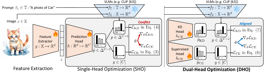
Figure 3: Conceptual illustration on KD frameworks, Single-Head Optimization (SHO) and Dual-Head Optimization (DHO), for semi-supervised settings. As demonstrated in Figure˜4, we observe gradient conflict of SHO. In contrast, DHO mitigates such conflicts by leveraging dual-head architectures.

Single-head KD baselines.

Building upon traditional KD approaches Hinton (2015), numerous studies have explored semi-supervised KD Chen et al. (2020b); He et al. (2021); Du et al. (2023); Yang et al. (2024b), unsupervised KD using self-supervised teacher models Fang et al. (2021c); Abbasi Koohpayegani et al. (2020); Navaneet et al. (2021); Wang et al. (2022); Xu et al. (2021); Singh and Wang (2025), and KD from VLMs Fang et al. (2021b); Wu et al. (2023); Sun et al. (2023b); Yang et al. (2024a); Vasu et al. (2024); Udandarao et al. (2024); Yang et al. (2024c), to name just a few. Our method builds on simple logit distillation in semi-supervised settings Hinton (2015); Chen et al. (2020b) that combines supervised loss $\mathcal{L}_{\text{CE}}$ on the labeled dataset $\mathcal{D}^{(l)}$ with KD loss $\mathcal{L}_{\text{KD}}$ on both labeled and unlabeled datasets $\mathcal{D}^{(l)}\cup\mathcal{D}^{(u)}$, i.e., $\lambda\mathcal{L}_{\text{CE}}+(1-\lambda)\mathcal{L}_{\text{KD}}$, where $\lambda\in[0,1]$ is a loss balancing hyperparameter. Specifically, the supervised loss $\mathcal{L}_{\text{CE}}$ and KD loss $\mathcal{L}_{\text{KD}}$ are defined as follows:

$$\mathcal{L}_{\text{CE}} =\frac{1}{N}\sum_{n}\ell\left(\sigma(h(z_{n}^{(l)})),y_{n}\right),$$ (2)

$$\mathcal{L}_{\text{KD}} =\frac{1}{N}\sum_{n}D_{\mathrm{KL}}\left[p_{n}^{(l)}\|\sigma(h(z_{n}^{(l)}))\right]+\frac{1}{M}\sum_{m}D_{\mathrm{KL}}\left[p_{m}^{(u)}\|\sigma(h(z_{m}^{(u)}))\right],$$ (3)

where $\ell$ denotes $D_{\mathrm{KL}}$ represent cross-entropy and Kullback-Leibler divergence, respectively. $z_{n}^{(l)}=g(x_{n}^{(l)})$ and $z_{m}^{(u)}=g(x_{m}^{(u)})\in\mathbb{R}^{d}$ are feature representations obtained by the feature extractor $g$. $p_{n}^{(l)}$ and $p_{m}^{(u)}\in\Delta^{C-1}$ are the categorical probability vectors of labeled $x_{n}^{(l)}$ and unlabeled data $x_{m}^{(u)}$, respectively, obtained by teacher VLM encoders $f_{\mathbb{X}}$ and $f_{\mathbb{T}}$, as described in Eq. 1. To optimize the parameters of $g$ and $h$, we use a mini-batch version of the above objective with stochastic gradient descent. Another well-studied single-head KD baseline is feature distillation, which leverages mean squared error (MSE) loss to directly align feature representations of student $g$ and teacher $f_{\mathbb{X}}$. We defer the details of feature distillation for VLMs to CLIP-KD Yang et al. (2024a).

3.2 Dual-Head Optimization (DHO)

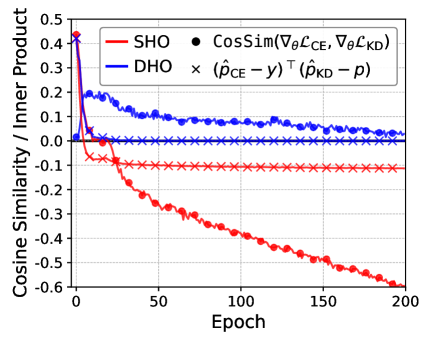
Figure 4: The average cosine similarity and inner product across 10 datasets. $\hat{p}_{\text{CE}}=\hat{p}_{\text{KD}}=\sigma(h(z))$ for SHO.

Gradient conflicts in single-head KD.

One of the single-head KD baselines, logit distillation, described in §3.1, offers a simple and efficient approach for transferring knowledge from VLMs in semi-supervised settings. However, we observe that its performance gain is suboptimal, which we attribute to gradient conflicts between the supervised and KD loss signals—a phenomenon well known to hinder effective feature representations in multi-task learning literature Yu et al. (2020); Liu et al. (2021); Chen and Er (2025). As illustrated in of Figure˜4, the parameter vector $\theta$ of feature extractor $g$ suffers from this issue: the cosine similarity between the gradients often turns negative, i.e., $\mathtt{CosSim}(\nabla_{\theta}\mathcal{L}_{\text{CE}},\nabla_{\theta}\mathcal{L}_{\text{KD}})<0$, indicating misaligned optimization directions.

Gradient analysis of single-head KD.

To understand this, we analyze the gradient w.r.t feature representation $z$. We denote $h(z)=Wz+b$, where $W\in\mathbb{R}^{C\times d}$, $b\in\mathbb{R}^{C}$, and $\hat{p}=\sigma(h(z))$. Then, gradients for a labeled data and their cosine similarity are:

$$\nabla_{z}\mathcal{L}_{\text{CE}}=W^{\top}(\hat{p}-y),\quad\nabla_{z}\mathcal{L}_{\text{KD}}=W^{\top}(\hat{p}-p),$$ (4)

$$\mathtt{CosSim}(\nabla_{z}\mathcal{L}_{\text{CE}},\nabla_{z}\mathcal{L}_{\text{KD}})=\frac{(\hat{p}-y)^{\top}WW^{\top}(\hat{p}-p)}{||W^{\top}(\hat{p}-y)||_{2}\cdot||W^{\top}(\hat{p}-p)||_{2}}.$$ (5)

$y$ denotes the one-hot ground-truth label and $p$ the teacher prediction. In few-shot settings, labeled data is scarce, making supervised signals noisy, while teacher predictions reflect pretraining priors that may not align with the limited labels. This mismatch often leads to a prediction-level conflict, indicated by $(\hat{p}-y)^{\top}(\hat{p}-p)<0$, which rapidly falls below zero during training ( in Figure˜4). As the dominant eigenvalue of $WW^{\top}$ grows to enhance class separability (Figure˜13-(left)), it amplifies the conflict magnitude, causing $\mathtt{CosSim}(\nabla_{z}\mathcal{L}_{\text{CE}},\nabla_{z}\mathcal{L}_{\text{KD}})$ to become strongly negative (Figure˜13-(right)). Eventually, this drives $\mathtt{CosSim}(\nabla_{\theta}\mathcal{L}_{\text{CE}},\nabla_{\theta}\mathcal{L}_{\text{KD}})$ down to $-0.6$ ( ).

Dual-head architecture.

To mitigate this issue, we propose to decouple the supervised and KD objectives via two independent prediction heads: $h_{\text{CE}}(z)=W_{\text{CE}}z+b_{\text{CE}}$ and $h_{\text{KD}}(z)=W_{\text{KD}}z+b_{\text{KD}}$, with $W_{\text{CE}},W_{\text{KD}}\in\mathbb{R}^{C\times d}$ and $b_{\text{CE}},b_{\text{KD}}\in\mathbb{R}^{C}$. The corresponding losses are:

$$\mathcal{L}_{\text{CE}} =\frac{1}{N}\sum_{n}\ell\left(\sigma(h_{\text{CE}}(z_{n}^{(l)})),y_{n}\right),$$ (6)

$$\mathcal{L}_{\text{KD}} =\frac{1}{N}\sum_{n}D_{\mathrm{KL}}\left[p_{n}^{(l)}\|\sigma(h_{\text{KD}}(z_{n}^{(l)}))\right]+\frac{1}{M}\sum_{m}D_{\mathrm{KL}}\left[p_{m}^{(u)}\|\sigma(h_{\text{KD}}(z_{m}^{(u)}))\right],$$ (7)

and the final loss is $\lambda\mathcal{L}_{\text{CE}}+(1-\lambda)\mathcal{L}_{\text{KD}}$, following single-head KD. Denoting $\hat{p}_{\text{CE}}=\sigma(h_{\text{CE}}(z))$ and $\hat{p}_{\text{KD}}=\sigma(h_{\text{KD}}(z))$, the gradients for a labeled data and their cosine similarity become:

$$\nabla_{z}\mathcal{L}_{\text{CE}}=W_{\text{CE}}^{\top}(\hat{p}_{\text{CE}}-y),\quad\nabla_{z}\mathcal{L}_{\text{KD}}=W_{\text{KD}}^{\top}(\hat{p}_{\text{KD}}-p),$$ (8)

$$\mathtt{CosSim}(\nabla_{z}\mathcal{L}_{\text{CE}},\nabla_{z}\mathcal{L}_{\text{KD}})=\frac{(\hat{p}_{\text{CE}}-y)^{\top}W_{\text{CE}}W_{\text{KD}}^{\top}(\hat{p}_{\text{KD}}-p)}{||W_{\text{CE}}^{\top}(\hat{p}_{\text{CE}}-y)||_{2}\cdot||W_{\text{KD}}^{\top}(\hat{p}_{\text{KD}}-p)||_{2}}.$$ (9)

Crucially, as shown in of Figure˜4, the prediction discrepancy term $(\hat{p}_{\text{CE}}-y)^{\top}(\hat{p}_{\text{KD}}-p)$ of DHO remains near zero throughout training. This is because the separated heads $h_{\text{CE}}$ and $h_{\text{KD}}$ are learned independently, without shared projections or alignment constraints. This is further supported by the high-dimensional geometry (e.g., $C>100$): random vectors drawn from a simplex or sphere tend to be nearly orthogonal due to the concentration of measure Vershynin (2018), resulting in weak correlation between their directions. Although spectral amplification occurs for $W_{\text{CE}}W_{\text{KD}}^{\top}$ (Figure˜13-(left)), the discrepancy term $(\hat{p}_{\text{CE}}-y)^{\top}(\hat{p}_{\text{KD}}-p)$ remains negligible, keeping $\mathtt{CosSim}(\nabla_{z}\mathcal{L}_{\text{CE}},\nabla_{z}\mathcal{L}_{\text{KD}})$ close to zero (Figure˜13-(right)). DHO thus maintains consistently positive gradient alignment, i.e., $\mathtt{CosSim}(\nabla_{\theta}\mathcal{L}_{\text{CE}},\nabla_{\theta}\mathcal{L}_{\text{KD}})>0$ (as shown in of Figure˜4), enabling stable and conflict-free representation learning. See Algorithm˜1 for the full training procedure of DHO.

Language-aware initialization and KD head alignment for VLM students.

We initialize the parameters of the dual heads $h_{\text{CE}}$ and $h_{\text{KD}}$, i.e., $W_{\text{CE}},W_{\text{KD}},b_{\text{CE}},b_{\text{KD}}$, using Kaiming initialization He et al. (2015). In the case of VLM-to-VLM distillation, however, we can leverage the teacher’s text encoder $f_{\mathbb{T}}$. Following prior work on language-aware initialization Li et al. (2022), we initialize the weights as $W_{\text{CE}},W_{\text{KD}}\leftarrow[f_{\mathbb{T}}(t_{1}),\ldots,f_{\mathbb{T}}(t_{C})]^{\top}\in\mathbb{R}^{C\times d}$. Furthermore, we align the prediction logic of KD head with that of teacher as follows:

$$h_{\text{KD}}=\frac{1}{\zeta}[\mathtt{CosSim}(g(x),w_{1}),\ldots,\mathtt{CosSim}(g(x),w_{C})]^{\top}\in\mathbb{R}^{C},$$ (10)

where $w_{c}\in\mathbb{R}^{d}$ denotes the $c$-th row of $W_{\text{KD}}$. This alignment encourages the KD head to mimic the teacher’s cosine similarity-based prediction behavior, leading to more stable distillation and improved performance, as shown in Table˜5.

Dual-heads interpolation for inference.

We propose a simple yet effective inference strategy for dual-head models by linearly interpolating:

$$\hat{p}=\alpha\cdot\sigma(h_{\text{CE}}(z))+(1-\alpha)\cdot\sigma(h_{\text{KD}}(z)/\beta)\in\Delta^{C-1},$$ (11)

where $\alpha\in[0,1]$ is an interpolation hyperparameter that balances the influence of the supervised and KD heads, and $\beta\in\mathbb{R}_{>0}$ is a temperature parameter that softens the KD logits. The final prediction is obtained via $\arg\max_{c\in[C]}\hat{p}_{c}$. This interpolation scheme is inspired by the mixture-of-experts (MoE) paradigm Jacobs et al. (1991), where multiple predictive sources are combined, and their relative importance is adjusted based on task conditions. In our setting, $\alpha$ allows flexible weighting of the two heads depending on which source—supervised labels or teacher predictions—offers more reliable guidance for a given dataset. This balance can be tuned using a validation set to reflect dataset-specific supervision quality and teacher accuracy. See Algorithm˜2 for the detailed inference process of DHO.

4 Experiments

We now elaborate the empirical effectiveness of the proposed method DHO. We first detail experimental setups in §4.1, and report the following empirical findings in §4.2:

• [F1]: In comparison to single-head KD baselines, DHO is an effective framework for semi-supervised settings, with negligible additional computational cost.

• [F2]: The improvement of DHO is attributed to gradient conflict mitigation, which leads to better feature representations compared to single-head KD baselines.

• [F3]: The proposed dual-heads output probability interpolation for inference further improves the performance of DHO on top of its enhanced feature representations.

• [F4]: DHO achieves state-of-the-art performance on ImageNet under low-shot semi-supervised settings, while using fewer parameters.

4.1 Experimental Setups

Datasets.

We use 11 diverse image classification datasets, including generic object recognition such as ImageNet Russakovsky et al. (2015), Caltech101 Fei-Fei et al. (2004) and other widely-adopted benchmarks for fine-grained classification (Cars Krause et al. (2013), Flowers102 Nilsback and Zisserman (2008), FGVCAircraft Maji et al. (2013), OxfordPets Parkhi et al. (2012)), domain-specific recognition (Food101 Bossard et al. (2014)), scene understanding (SUN397 Xiao et al. (2010)), texture analysis (DTD Cimpoi et al. (2014)), satellite imagery (EuroSAT Helber et al. (2019)), and human actions (UCF101 Soomro (2012)). See Appendix˜C for details.

Baselines.

We first compare DHO with conventional single-head KD baselines; CE: we train a model only on labeled dataset $\mathcal{D}^{(l)}$ with cross entropy loss (Eq. 2), KD (logit): on unlabeled dataset $\mathcal{D}^{(u)}$ with logit distillation (Eq. 3), and KD (feature): on $\mathcal{D}^{(u)}$ with feature distillation Yang et al. (2024a). We train a model on both $\mathcal{D}^{(l)}$ and $\mathcal{D}^{(u)}$ with CE+KD (logit) or CE+KD (feature): which combines CE with each KD variant with the balancing hyperparameter $\lambda$. We also consider existing dual-head KD approaches: SSKD He et al. (2021) uses dual-heads, with each head trained on labeled and unlabeled sets respectively, assuming different data distributions between them, and DHKD Yang et al. (2024d) introduces binary KD loss working on logits before softmax to prevent neural collapse Papyan et al. (2020), but both methods predict labels using only $h_{\text{CE}}$. We further compare DHO with state-of-the-art methods on ImageNet with low-shot semi-supervised settings, including self and semi-supervised learning Zheng et al. (2023); Assran et al. (2021); Chen et al. (2020b, b); Assran et al. (2022); Cai et al. (2022, 2022), CLIP-based-training Li et al. (2022); Liu et al. (2023), co-training Rothenberger and Diochnos (2023), KD Chen et al. (2020b), and zero-shot VLMs Zhai et al. (2023); Fang et al. (2023).

Architecture choices for teacher and student models.

For zero-shot teachers, we use CLIP ResNet-50 Radford et al. (2021) in few-shot settings and VIT-H/14 from DFN Fang et al. (2023) in low-shot settings. For few-shot teachers, we adopt Tip-Adapter-F Zhang et al. (2021), a learnable adapter model, and denote the corresponding variant as DHO-F. Student models are initialized from pretrained checkpoints Turc et al. (2019). On ImageNet, to avoid label leakage, we either train ResNet-18 from scratch or use a self-supervised ResNet-50 from DINO Caron et al. (2021). For other datasets, we use ResNet-18 and MobileNetV2 Sandler et al. (2018) without such concerns. In low-shot settings, we use CLIP ViT-B/16 and ViT-L/14 Radford et al. (2021). See Table˜6 for an overview.

Implementation details.

We consider few-shot (1, 2, 4, 8, 16-shot) and low-shot (1% or 10%) settings, treating the rest as unlabeled. Prompt templates follow Tip-Adapter Zhang et al. (2021). As detailed in §3.2, we use linear heads for all methods; additional analysis on non-linear heads is provided in Section˜E.2. All methods use consistent hyperparameters, including $\zeta=0.01$, $\lambda=0.5$, and others. For KD (feature) baselines, we scale the MSE loss to match $\mathcal{L}_{\text{CE}}$ following Yang et al. (2024a). $\alpha$ and $\beta$ of DHO are tuned on validation sets. When validation data is unavailable (e.g., ImageNet), we fix $\beta=0.5$ across all settings. We heuristically set $\alpha=0.4$ for zero-shot teachers and $\alpha=0.2$ for few-shot teachers, reflecting the latter’s higher reliability. In low-shot settings, we use $\alpha=0.5$ due to increased label availability. Results are from a single run due to limited compute. See Section˜B.2 for more details.

4.2 Experimental Results

Table 1: Results on ImageNet under few-shot semi-supervision using ResNet-18 and ResNet-50.

	ResNet-18 trained from scratch						Self-supervised ResNet-50
Method	0-shot	1-shot	2-shot	4-shot	8-shot	16-shot	0-shot	1-shot	2-shot	4-shot	8-shot	16-shot
Single-head KD methods
KD	51.0	-	-	-	-	-	61.0	-	-	-	-	-
CE	-	0.7	1.1	1.8	3.4	8.2	-	11.4	17.3	26.4	36.7	47.0
CE+KD (feature) Yang et al. (2024a)	-	17.1	23.5	28.0	32.2	33.8	-	23.0	32.3	41.3	48.2	54.3
CE+KD (logit) Chen et al. (2020b)	-	50.5	50.6	50.6	51.0	51.2	-	60.4	60.8	61.2	61.6	62.3
Dual-head KD methods
DHO (zero-shot teacher Radford et al. (2021))	-	51.8	52.4	52.6	53.3	54.5	-	61.0	62.1	62.5	63.7	64.7
DHO-F (few-shot teacher Zhang et al. (2021))	-	53.7	54.2	54.8	56.2	57.7	-	62.3	63.1	63.9	65.5	66.8
Teacher Models
CLIP Radford et al. (2021)	50.0	-	-	-	-	-	60.3	-	-	-	-	-
Tip-Adapter-F Zhang et al. (2021)	-	52.0	52.4	53.2	54.0	55.3	-	61.0	61.6	62.5	63.8	65.4

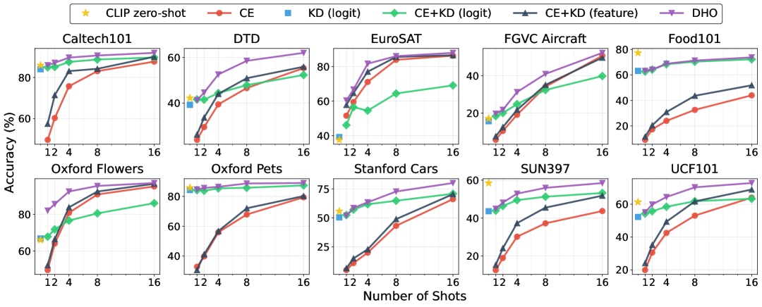
Figure 5: Results on 10 datasets under few-shot semi-supervision using ResNet-18 with zero-shot teacher Radford et al. (2021).

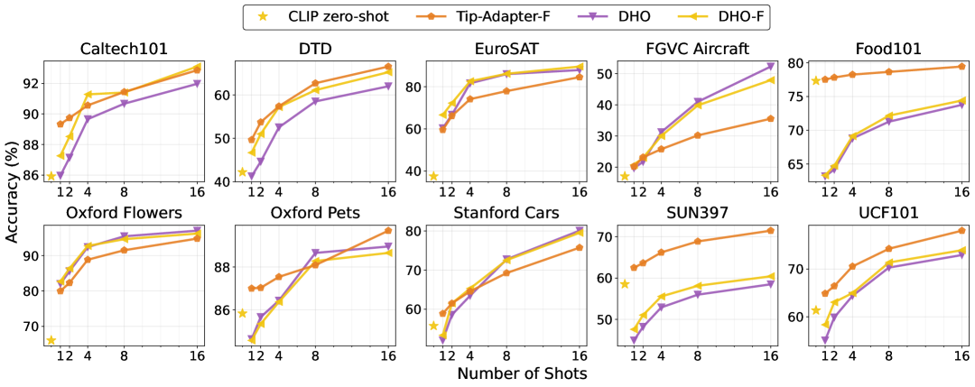
Figure 6: Results on 10 datasets using ResNet-18 with either zero- or few-shot teacher Zhang et al. (2021).

Table 2: Inference overhead using RTX 4090.

Model	Params	FLOPs	Throughput
	(M)	(G)	(im/s)
ResNet-18	11.69	1.83	3525.7
+ DHO	12.20 (+4.4%)	1.83 (+0.0%)	3518.6 (-0.20%)
ResNet-50	25.56	4.14	1018.4
+ DHO	27.61 (+8.0%)	4.15 (+0.2%)	1016.4 (-0.20%)

[F1]: Effectiveness of DHO compared to SHO.

We first compare DHO with SHO on ImageNet under 1, 2, 4, 8, and 16-shot settings using ResNet-18 (trained from scratch) and self-supervised ResNet-50. As shown in Table˜1, DHO consistently outperforms SHO, with further gains from DHO-F that incorporates few-shot teachers. We also compare against dual-head KD methods on ResNet-50: SSKD and DHKD achieve 55.2/58.1/60.0/62.3/64.0 and 25.6/34.8/42.7/49.2/55.2, respectively, while DHO surpasses both across all shot counts. To assess generality, we evaluate on 10 additional datasets using ResNet-18. DHO consistently outperforms SHO, with larger improvements from few-shot teachers (Figures˜5 and 6). Results for MobileNetV2 are shown in Figures˜12 and 12. Table˜2 shows these gains incur minimal overhead in FLOPs and throughput, especially on ImageNet and negligible for smaller datasets with fewer classes ($C<1000$). See inference overhead for MobileNetV2, ViT-B/16, and ViT-L/14 in Table˜7.

Table 3: Linear evaluation results.

Method	Top-1 (%)	Top-5 (%)
CE+KD (feature) Yang et al. (2024a)	62.3	85.0
CE+KD (logit) Chen et al. (2020b)	66.2	88.8
DHO	67.1	89.3

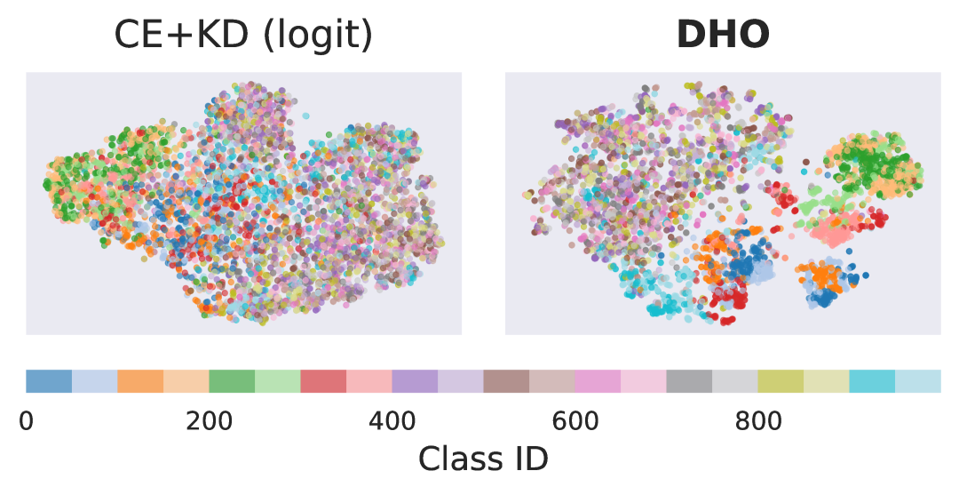
Figure 7: t-SNE visualization.

[F2]: Enhanced feature representation of DHO.

To validate our claim that mitigating gradient conflicts improves feature representations, we evaluate features using the standard linear evaluation protocol Chen et al. (2020b). We train CE+KD (feature), CE+KD (logit), and DHO under the 16-shot semi-supervised setting on ImageNet, freeze the feature extractor $g$, and train a new prediction linear head $h_{\text{LE}}$ on top of $g$ using fully labeled data. As shown at the top of Section˜4.2, DHO achieves higher Top-1 and Top-5 accuracy than other methods. To further assess feature quality, we visualize embeddings $z$ using t-SNE Van der Maaten and Hinton (2008) in Figure˜7. Compared to the CE+KD (logit) baseline, DHO produces more compact and class-separated feature clusters. These results support our claim that DHO enhances feature representations by mitigating gradient conflicts; this improvement leads to better performance compared to SHO, as discussed in [F1] and illustrated in Table˜1, Figures˜5, 6, 12 and 12.

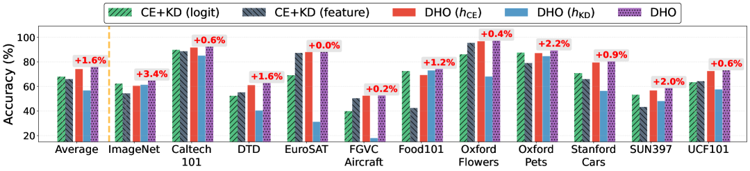
Figure 8: Results of ablation studies on dual-heads interpolation strategy in Eq. 11 of DHO.

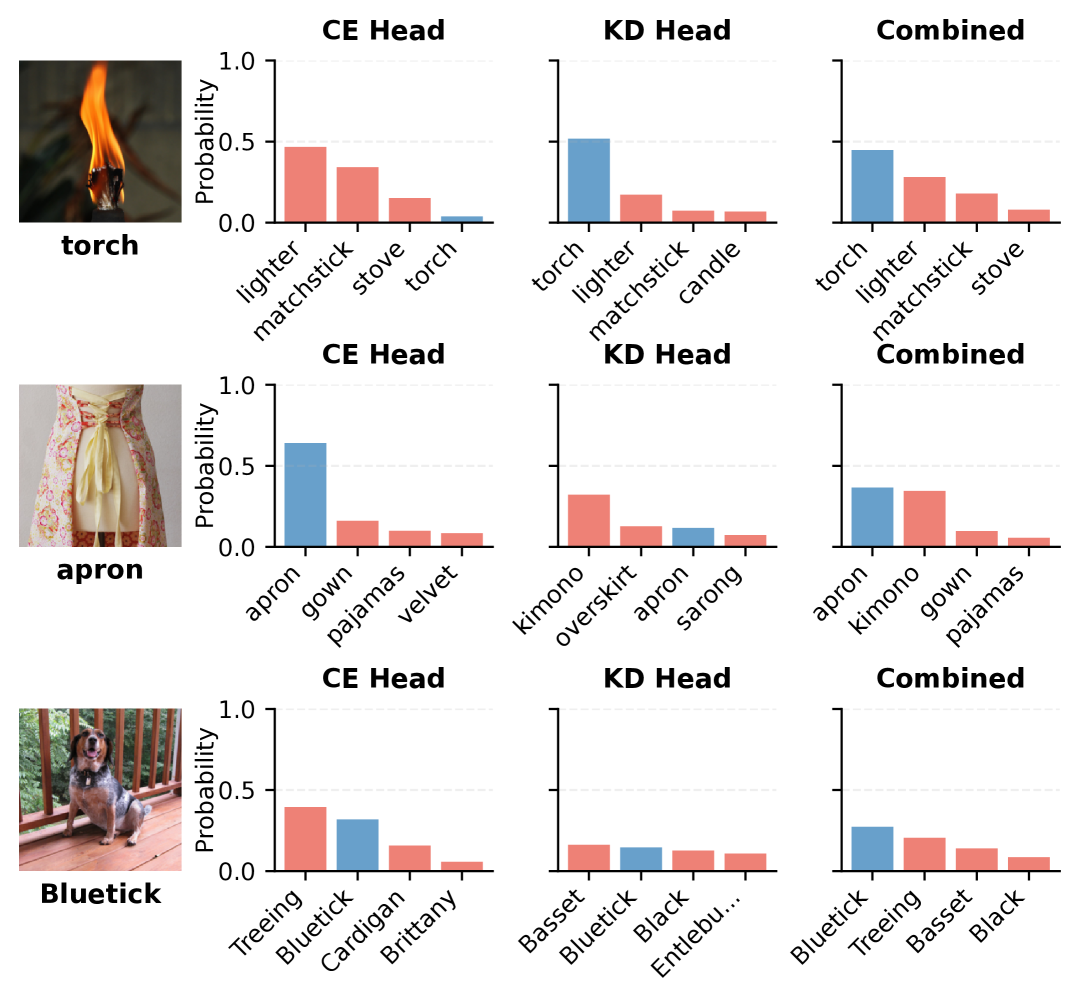
Figure 9: Qualitative results on challenging cases.

[F3]: Effectiveness of dual-head interpolation.

We evaluate the effectiveness of dual-head interpolation (Eq. 11) by comparing DHO with CE+KD (logit), CE+KD (feature), and ablations DHO ($h_{\text{CE}}$) and DHO ($h_{\text{KD}}$), which predict using only one head, i.e., $\alpha=1$ or $0$. We use ResNet-50 for ImageNet and ResNet-18 for the other datasets. As shown in Figure˜8, DHO outperforms DHO ($h_{\text{CE}}$) by an average of 1.6% across 11 datasets, with a maximum gain of +3.4% on ImageNet and no degradation on any dataset. Since $\alpha$ and $\beta$ are inference-time hyperparameters, dual-head interpolation introduces minimal overhead while consistently improving or maintaining performance. We further conduct case studies on its effect. Figure˜9 illustrates three challenging examples: CE head ($h_{\text{CE}}$) is correct in the first, KD head ($h_{\text{KD}}$) in the second, and both fail in the third case, yet the proposed combined prediction is correct—demonstrating the ability of DHO to resolve individual head failures. See additional analysis in Section˜E.3.

Table 4: Results on ImageNet under low-shot settings. For CT and MCT methods, numbers in parentheses indicate the number of different architectures for co-training.

Method	Architecture	Params	1%	10%
		(M)	(%)	(%)
Self and Semi-supervised Learning
MSN Assran et al. (2022)	ViT-B/4	86	75.7	80.2
Semi-ViT Cai et al. (2022)	ViT-L/14	307	77.3	83.3
Semi-ViT Cai et al. (2022)	ViT-H/14	632	80.0	84.3
CLIP-based Training
CLIP Li et al. (2022)	ViT-B/16	86	74.3	80.4
REACT Liu et al. (2023)	ViT-B/16	86	76.1	80.8
REACT (Gated-Image) Liu et al. (2023)	ViT-B/16	129	77.4	81.8
CLIP Li et al. (2022)	ViT-L/14	304	80.5	84.7
REACT Liu et al. (2023)	ViT-L/14	304	81.6	85.1
REACT (Gated-Image) Liu et al. (2023)	ViT-L/14	380	81.6	85.0
Co-training based Methods
CT Rothenberger and Diochnos (2023)	Multi-arch (2)	608	80.1	85.1
MCT Rothenberger and Diochnos (2023)	Multi-arch (2)	608	80.7	85.2
CT Rothenberger and Diochnos (2023)	Multi-arch (4)	1071	80.0	84.8
MCT Rothenberger and Diochnos (2023)	Multi-arch (4)	1071	80.5	85.8
Knowledge Distillation
SimCLR v2 distill Chen et al. (2020b)	ResNet-50 (2×+SK)	140	75.9	80.2
SimCLR v2 self-distill Chen et al. (2020b)	ResNet-154 (3×+SK)	795	76.6	80.9
DHO (ours)	ViT-B/16	86	81.6	82.8
DHO (ours)	ViT-L/14	304	84.6	85.9
Zero-shot VLMs
SigLIP Zhai et al. (2023)	ViT-SO400M/14	400	83.1	-
DFN Fang et al. (2023)	ViT-H/14	632	84.4	-

Table 5: Results of ablation studies on language-aware initialization and KD-head alignment for VLM students on ImageNet with 1% labeled data.

Init ($h_{\text{CE}}$/$h_{\text{KD}}$).	Align.	Accuracy (%)
✗ / ✗	✗	78.3
✓ / ✗	✗	78.5 (+0.2)
✓ / ✓	✗	78.6 (+0.3)
✓ / ✓	✓	78.7 (+0.4)

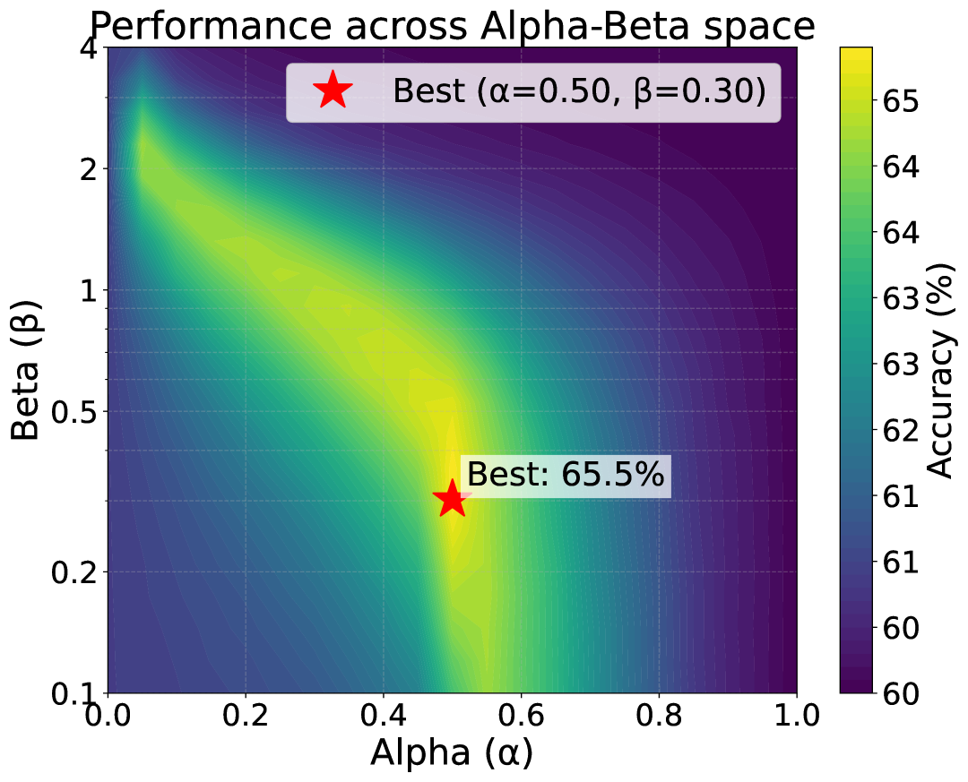
Figure 10: Visualization of grid search results for $\alpha$ and $\beta$ using ResNet-50 on ImageNet under the 16-shot semi-supervised setting.

[F4]: DHO achieves SoTA performance on ImageNet under low-shot settings.

We compare DHO to previous state-of-the-art (SoTA) methods on ImageNet under 1% and 10% labeled data. All results are taken from published papers, except for DHO. As shown in Section˜4.2, DHO with ViT-L/14 surpasses the previous SoTA by 3% (1% data) and 0.1% (10% data), while using 218M and 767M fewer parameters, respectively. Notably, DHO achieves 81.6% accuracy with only 86M parameters—the same as REACT Liu et al. (2023) using 304M. These results show that DHO is a simple yet effective method.

Effectiveness of language-aware initialization and KD head alignment.

Table˜5 shows ablation results on language-aware initialization (Init.) and KD-head alignment (Align.) on ImageNet (1%). We use ViT-B/16 student and ViT-L/14 teacher for computational efficiency. We observe that applying Init. on each head independently improves performance, and applying Align. further enhances it.

Effect of $\alpha$ and $\beta$.

To understand how $\alpha$ and $\beta$ in DHO affect performance, we visualize grid search results on ImageNet with ResNet-50 under the 16-shot setting. Figure˜10 shows performance peaks at balanced heads ($\alpha\approx 0.5$) and degrades at extreme values ($\alpha\approx 0$ or $1$) regardless of $\beta$. With balanced heads, performance remains stable for $\beta\in[0.1,1]$, optimizing around $\beta=0.3$. Furthermore, under mild assumptions, Appendix˜A shows that DHO $\epsilon$-approximates SHO w.r.t the $\ell_{1}$ norm by setting $\alpha=\lambda$ and $\beta=\tau$, where $\tau$ is the corresponding temperature hyperparameter for $\beta$ in SHO. Notably, $\lambda$ and $\tau$ are training hyperparameters, while $\alpha$ and $\beta$ are inference hyperparameters. This allows DHO to emulate the effects of tuning hyperparameters of SHO without retraining.

OOD generalization.

Although this paper focuses on in-distribution generalization, we also evaluate DHO on ImageNet-based out-of-distribution (OOD) benchmarks Recht et al. (2019); Wang et al. (2019); Hendrycks et al. (2021b, a). Due to page limits, we present the details in Section˜D.2; in summary, combining DHO with VPT Jia et al. (2022), CoOP Zhou et al. (2022b), and PromptSRC Khattak et al. (2023b) consistently improves their OOD performance.

Training cost and inference efficiency with ToMe.

Table˜8 reports the training cost of DHO, and Table˜9 shows ToMe Bolya et al. (2022) significantly reduces inference overhead with minimal performance drop.

5 Conclusion, Limitation, and Future Work

We presented DHO, a framework that leverages both labeled samples and teacher predictions for knowledge distillation from pretrained VLMs in semi-supervised settings. Through [F1–4], we empirically demonstrated that DHO is a simple yet effective approach. However, our work is currently limited to image classification tasks. Future work could extend DHO to other computer vision and multimodal tasks, such as object detection, segmentation, and language modeling. With suitable architectural adaptations, we believe the dual-head design of DHO can facilitate efficient knowledge transfer from foundation models across a broader range of applications.

Appendix Overview

This appendix provides supplementary material to support the main paper and is organized as follows:

• Theoretical Analysis (Appendix˜A): provides mathematical foundations and theoretical guarantees for our approach.

• Algorithms and Implementation (Appendix˜B): presents detailed pseudocode (Section˜B.1), implementation specifics (Section˜B.2), and computational overhead analysis (Section˜B.3).

• Datasets (Appendix˜C): describes the datasets used in our experiments, including statistics and preprocessing details.

• Additional Experiments (Appendix˜D): presents MobileNet experiments (Section˜D.1) and out-of-distribution generalization results (Section˜D.2).

• Additional Analyses (Appendix˜E): contains gradient analysis (Section˜E.1), non-linear head design studies (Section˜E.2), and further dual-head investigations (Section˜E.3).

Appendix A Theoretical Analysis

In this section, we provide a theoretical analysis of our Dual-Head Optimization (DHO) framework. We establish that DHO effectively addresses single-head logit distillation Hinton [2015], Chen et al. [2020b] by decoupling conflicting gradients through specialized heads during training. We prove that post-training, the optimal prediction from our dual-head model—formulated as a weighted combination of the heads’ outputs—is mathematically equivalent to the optimal solution of conventional single-head distillation. This equivalence provides theoretical justification for our approach while eliminating gradient conflicts. Furthermore, DHO enables efficient adaptation to various datasets through tunable hyperparameters ($\alpha$ and $\beta$) without requiring model retraining. Note that in this section we slightly abuse the notation of the main paper for clarity, e.g., we denote $p_{\tau}$ as teacher predictions with temperature scaling $\tau$.

A.1 Single-Head Optimization

We begin by considering two target probability distributions: the ground truth label distribution $y$ and the teacher’s softened distribution $p_{\tau}$ for input $x\in\mathcal{X}$, where:

• $y$ represents the ground truth label distribution, typically one-hot encoded vectors where $y_{c}=1$ for the true class $c$ and 0 elsewhere

• $p_{\tau}$ denotes the teacher’s softened distribution with temperature scaling: $p_{\tau}=\sigma(z_{t}/\tau)$, where $z_{t}$ represents the teacher’s logits and $\sigma$ is the softmax function

Theorem A.1 (Optimal Distribution for Single-Head Optimization).

The distribution $\hat{p}^{*}$ that minimizes the weighted combination of cross-entropy loss with respect to $y$ and Kullback-Leibler divergence with respect to $p_{\tau}$:

$$\mathcal{L}(\hat{p})=\lambda\ell(\hat{p},y)+(1-\lambda)D_{\mathrm{KL}}(p_{\tau}\|\hat{p})$$ (12)

is given by the weighted arithmetic mean:

$$\hat{p}^{*}=\lambda y+(1-\lambda)p_{\tau}$$ (13)

where $\lambda\in[0,1]$ is the weighting hyperparameter.

Proof.

We begin by expanding the objective function:

$$\mathcal{L}(\hat{p}) =\lambda\ell(\hat{p},y)+(1-\lambda)D_{\mathrm{KL}}(p_{\tau}\|\hat{p})$$ (14)

$$=-\lambda\sum_{c=1}^{C}y_{c}\log\hat{p}_{c}+(1-\lambda)\sum_{c=1}^{C}p_{\tau,c}\log\frac{p_{\tau,c}}{\hat{p}_{c}}$$ (15)

$$=-\lambda\sum_{c=1}^{C}y_{c}\log\hat{p}_{c}+(1-\lambda)\sum_{c=1}^{C}p_{\tau,c}\log p_{\tau,c}-(1-\lambda)\sum_{c=1}^{C}p_{\tau,c}\log\hat{p}_{c}$$ (16)

$$=-\sum_{c=1}^{C}[\lambda y_{c}+(1-\lambda)p_{\tau,c}]\log\hat{p}_{c}+(1-\lambda)\sum_{c=1}^{C}p_{\tau,c}\log p_{\tau,c}$$ (17)

Since the last term is constant with respect to $\hat{p}$, the optimization problem reduces to minimizing:

$$\mathcal{L}^{\prime}(\hat{p})=-\sum_{c=1}^{C}[\lambda y_{c}+(1-\lambda)p_{\tau,c}]\log\hat{p}_{c}$$ (18)

Subject to the probability constraints:

$$\sum_{c=1}^{C}\hat{p}_{c}=1,\quad\hat{p}_{c}\geq 0\quad\forall c\in\{1,2,\ldots,C\}$$ (19)

Applying the method of Lagrange multipliers with multiplier $\mu$:

$$\mathcal{L}(\hat{p},\mu)=-\sum_{c=1}^{C}[\lambda y_{c}+(1-\lambda)p_{\tau,c}]\log\hat{p}_{c}+\mu\left(\sum_{c=1}^{C}\hat{p}_{c}-1\right)$$ (20)

Taking the partial derivative with respect to $\hat{p}_{c}$ and setting it to zero:

$$-\frac{\lambda y_{c}+(1-\lambda)p_{\tau,c}}{\hat{p}_{c}}+\mu=0$$ (21)

Solving for $\hat{p}_{c}$:

$$\hat{p}_{c}=\frac{\lambda y_{c}+(1-\lambda)p_{\tau,c}}{\mu}$$ (22)

Using the constraint $\sum_{c=1}^{C}\hat{p}_{c}=1$, and observing that $\sum_{c=1}^{C}y_{c}=1$ and $\sum_{c=1}^{C}p_{\tau,c}=1$ (both being probability distributions):

$$\sum_{c=1}^{C}\hat{p}_{c}=\sum_{c=1}^{C}\frac{\lambda y_{c}+(1-\lambda)p_{\tau,c}}{\mu}=1$$ (23)

$$\frac{1}{\mu}\sum_{c=1}^{C}[\lambda y_{c}+(1-\lambda)p_{\tau,c}]=1$$ (24)

$$\frac{1}{\mu}[\lambda\sum_{c=1}^{C}y_{c}+(1-\lambda)\sum_{c=1}^{C}p_{\tau,c}]=1$$ (25)

$$\frac{1}{\mu}[\lambda+(1-\lambda)]=1$$ (26)

$$\mu=1$$ (27)

Therefore, the optimal solution is:

$$\hat{p}^{*}_{c}=\lambda y_{c}+(1-\lambda)p_{\tau,c}$$ (28)

This weighted arithmetic mean of the two target distributions is the optimal solution that minimizes our objective function. ∎

A.2 Dual-Head Optimization

In our proposed Dual-Head Optimization (DHO) framework, we extract shared features $g(x)$ from input $x$ and apply two specialized classification heads:

• $h_{\text{CE}}(z)=W_{\text{CE}}z+b_{\text{CE}}$: optimized exclusively to match ground truth labels using cross-entropy loss $\ell(\sigma(h_{\text{CE}}(z)),y)$

• $h_{\text{KD}}(z)=W_{\text{KD}}z+b_{\text{KD}}$: optimized exclusively to match teacher predictions using KL divergence $D_{\mathrm{KL}}(p_{\tau}\|\sigma(h_{\text{KD}}(z)/\beta))$

where $z=g(x)$ is the feature representation, and the parameter $\beta$ controls the temperature during inference, while a fixed temperature of 1 is used during training of the knowledge distillation head.

Assumption A.2 ($\varepsilon$-Convergence).

We assume that after sufficient training, both heads have converged to their respective target distributions with bounded error:

$$\sup_{x}\|\sigma(h_{\text{CE}}(z))-y\|_{1}\leq\varepsilon,\quad\sup_{x}\|\sigma(h_{\text{KD}}(z)/\beta)-p_{\tau}\|_{1}\leq\varepsilon$$ (29)

where $\|\cdot\|_{1}$ denotes the $\ell_{1}$ norm and $\varepsilon>0$ is a small constant.

Theorem A.3 (Inference Equivalence Under $\varepsilon$-Convergence).

Under ˜A.2, by combining the outputs of both heads as:

$$\hat{p}_{\texttt{DHO}}=\alpha\cdot\sigma(h_{\text{CE}}(z))+(1-\alpha)\cdot\sigma(h_{\text{KD}}(z)/\beta),\quad\text{where }\alpha=\lambda$$ (30)

we obtain a prediction that approximates the optimal single-head solution with bounded error:

$$\|\hat{p}_{\texttt{DHO}}-\hat{p}^{*}\|_{1}\leq\varepsilon$$ (31)

Proof.

We analyze the $\ell_{1}$ distance between the DHO prediction and the optimal solution:

$$\|\hat{p}_{\texttt{DHO}}-\hat{p}^{*}\|_{1} =\|\alpha\cdot\sigma(h_{\text{CE}}(z))+(1-\alpha)\cdot\sigma(h_{\text{KD}}(z)/\beta)-\lambda y-(1-\lambda)p_{\tau}\|_{1}$$ (32)

$$=\|\lambda(\sigma(h_{\text{CE}}(z))-y)+(1-\lambda)(\sigma(h_{\text{KD}}(z)/\beta)-p_{\tau})\|_{1}$$ (33)

$$\leq\lambda\|\sigma(h_{\text{CE}}(z))-y\|_{1}+(1-\lambda)\|\sigma(h_{\text{KD}}(z)/\beta)-p_{\tau}\|_{1}$$ (34)

$$\leq\lambda\varepsilon+(1-\lambda)\varepsilon=\varepsilon$$ (35)

where we applied the triangle inequality for the $\ell_{1}$ norm and used ˜A.2.

Therefore, we have established that:

$$\hat{p}_{\texttt{DHO}}\approx_{\varepsilon}\hat{p}^{*}$$ (36)

where $\approx_{\varepsilon}$ denotes approximation with $\ell_{1}$ error bound $\varepsilon$. ∎

Lemma A.4 (Temperature Matching via KL Divergence).

Assume the knowledge distillation head is trained to minimize KL divergence with respect to the teacher’s predictions at temperature 1, such that:

$$D_{\mathrm{KL}}(p_{1}\|\sigma(h_{\text{KD}}(z)))\leq\delta$$ (37)

Then, setting the temperature parameter $\beta=\tau$ at inference time allows the KD head to approximate the teacher’s prediction at temperature $\tau$ with error bound:

$$\|\sigma(h_{\text{KD}}(z)/\beta)-p_{\tau}\|_{1}\leq\sqrt{2\delta}$$ (38)

Proof.

When logits are properly scaled and under appropriate conditions of the softmax function, we can reasonably approximate:

$$D_{\mathrm{KL}}(p_{\tau}\|\sigma(h_{\text{KD}}(z)/\tau))\approx D_{\mathrm{KL}}(p_{1}\|\sigma(h_{\text{KD}}(z)))\leq\delta$$ (39)

Applying Pinsker’s inequality, which establishes a relationship between KL divergence and the L1 norm difference between probability distributions:

$$\|p_{\tau}-\sigma(h_{\text{KD}}(z)/\tau)\|_{1}\leq\sqrt{2D_{\mathrm{KL}}(p_{\tau}\|\sigma(h_{\text{KD}}(z)/\tau))}\leq\sqrt{2\delta}$$ (40)

To ensure $\varepsilon$-convergence between the KD head at temperature $\tau$ and the teacher’s prediction at temperature $\tau$, it is sufficient to guarantee:

$$\sqrt{2\delta}\leq\varepsilon\Rightarrow\delta\leq\frac{\varepsilon^{2}}{2}$$ (41)

∎

Corollary A.5 (Optimal DHO Configuration).

With proper training ensuring $\varepsilon$-convergence of both heads, dual-head optimization with temperature parameter $\beta=\tau$ and mixing parameter $\alpha=\lambda$ approximates the optimal single-head objective with error bounded by $\varepsilon$:

$$\hat{p}_{\texttt{DHO}}\approx_{\varepsilon}\hat{p}^{*}=\lambda y+(1-\lambda)p_{\tau}$$ (42)

This demonstrates that our DHO approach achieves the same theoretical optimality as SHO.

Appendix B Algorithms and Implementation

B.1 Pseudocode

We present the pseudocode for DHO in Algorithms˜1 and 2 for training and inference, respectively.

Algorithm 1 DHO Training with zero-shot CLIP Radford et al. [2021] teacher

1: Input: labeled set $\mathcal{D}^{(l)}=\{(x^{(l)}_{i},y_{i})\}_{i=1}^{N}$, unlabeled set $\mathcal{D}^{(u)}=\{x^{(u)}_{j}\}_{j=1}^{M}$,

2: Input: student feature extractor $g$, prediction heads $h_{\text{CE}},h_{\text{KD}}$, teacher encoders $f_{\mathbb{X}},f_{\mathbb{T}}$,

3: Input: prompt template “A photo of [CLASS]”, temperature scaling factors $\zeta,\eta$,

4: Input: balancing hyperparameter $\lambda$,

5: Input: supervised mini-batch size $B$, and unsupervised mini-batch size $B^{\prime}$.

6: while not converged do

7:  Sample mini-batch $\mathcal{B}^{(l)}=\{(x_{b}^{(l)},y_{b})\}_{b=1}^{B}$ from $\mathcal{D}^{(l)}$, $\mathcal{B}^{(u)}=\{x_{b^{\prime}}^{(u)}\}_{b^{\prime}=1}^{B^{\prime}}$ from $\mathcal{D}^{(l)}\cup\mathcal{D}^{(u)}$.

8:  // Process labeled data

9:  for each $(x_{b}^{(l)},y_{b})\in\mathcal{B}^{(l)}$ do

10:   $z_{b}^{(l)}\leftarrow g(x_{b}^{(l)})$

11:   $\hat{p}_{\text{CE},b}^{(l)}\leftarrow\sigma(h_{\text{CE}}(z_{b}^{(l)}))$

12:   $\hat{p}_{\text{KD},b}^{(l)}\leftarrow\sigma(\frac{1}{\eta}h_{\text{KD}}(z_{b}^{(l)}))$

13:   $p_{b}^{(l)}\leftarrow\sigma\left(\frac{1}{\zeta\cdot\eta}[\mathtt{CosSim}(f_{\mathbb{X}}(x_{b}^{(l)}),f_{\mathbb{T}}(t_{1})),\ldots,\mathtt{CosSim}(f_{\mathbb{X}}(x_{b}^{(l)}),f_{\mathbb{T}}(t_{C}))]^{\top}\right)$

14:  end for

15:  // Process unlabeled data

16:  for each $x_{b^{\prime}}^{(u)}\in\mathcal{B}^{(u)}$ do

17:   $z_{b^{\prime}}^{(u)}\leftarrow g(x_{b^{\prime}}^{(u)})$

18:   $\hat{p}_{\text{KD},b^{\prime}}^{(u)}\leftarrow\sigma(\frac{1}{\eta}h_{\text{KD}}(z_{b^{\prime}}^{(u)}))$

19:   $p_{b^{\prime}}^{(u)}\leftarrow\sigma\left(\frac{1}{\zeta\cdot\eta}[\mathtt{CosSim}(f_{\mathbb{X}}(x_{b^{\prime}}^{(u)}),f_{\mathbb{T}}(t_{1})),\ldots,\mathtt{CosSim}(f_{\mathbb{X}}(x_{b^{\prime}}^{(u)}),f_{\mathbb{T}}(t_{C}))]^{\top}\right)$

20:  end for

21:  // Compute losses and update

22:  $\mathcal{L}_{\text{CE}}\leftarrow\frac{1}{B}\sum_{b=1}^{B}\ell(\hat{p}_{\text{CE},b}^{(l)},y_{b})$

23:  $\mathcal{L}_{\text{KD}}\leftarrow\frac{1}{B}\sum_{b=1}^{B}D_{\mathrm{KL}}(\hat{p}_{\text{KD},b}^{(l)}||p_{b}^{(l)})+\frac{1}{B^{\prime}}\sum_{b^{\prime}=1}^{B^{\prime}}D_{\mathrm{KL}}(\hat{p}_{\text{KD},b^{\prime}}^{(u)}||p_{b^{\prime}}^{(u)})$

24:  $\mathcal{L}\leftarrow\lambda\mathcal{L}_{\text{CE}}+(1-\lambda)\mathcal{L}_{\text{KD}}$

25:  Update parameters of $g$, $h_{\text{CE}}$, $h_{\text{KD}}$ using $\nabla\mathcal{L}$

26: end while

Algorithm 2 Dual-Head Optimization Inference

1: Input: an image $x$, feature extractor $g$, prediction heads $h_{\text{CE}},h_{\text{KD}}$, linear coefficient $\alpha$, temperature scaling $\beta$

2: $z\leftarrow g(x)$

3: $\hat{p}_{\text{CE}}\leftarrow\sigma(h_{\text{CE}}(z))$

4: $\hat{p}_{\text{KD}}\leftarrow\sigma(h_{\text{KD}}(z)/\beta)$

5: $\hat{p}\leftarrow\alpha\cdot\hat{p}_{\text{CE}}+(1-\alpha)\cdot\hat{p}_{\text{KD}}$

6: $\hat{y}\leftarrow\arg\max_{c}(\hat{p}_{c})$

7: Return: $\hat{y}$

B.2 Implementation Details

Table 6: Implementation details for our experiments across different settings.

Few-shot Semi-supervised Settings on ImageNet
Model Configuration	Student Training Details
• Student: ResNet18 He et al. [2016] from scratch or ResNet50 from DINO Caron et al. [2021] • Input size: 224$\times$224 • Zero-shot Teacher: ResNet50 from CLIP Radford et al. [2021] • Few-shot Teacher: ResNet50 from Tip-Adapter-F Zhang et al. [2021] • Teacher input size: 224$\times$224 • labeled data: $K\in\{1,2,4,8,16\}$ shots • $\zeta$, $\eta$, and $\lambda$: $0.01,2,0.5$ • $\alpha$ and $\beta$: $\alpha=0.4$, $\beta=0.5$ (zero-shot); $\alpha=0.2$, $\beta=0.5$ (few-shot)	• Epochs: 20 • Optimizer: AdamW ($\beta_{1}$=0.9, $\beta_{2}$=0.999) • Learning rate: $1\times 10^{-3}$, weight decay: $1\times 10^{-2}$ • Batch size: 512 (labeled: 256, unlabeled: 256) • Scheduler: Cosine decay without warmup • Augmentation: Random crops (x0.5-1.0), horizontal flips
Few-shot Semi-supervised Settings on 10 Fine-Grained Datasets
Model Configuration	Student Training Details
• Student: ResNet18 He et al. [2016] or MobileNet Sandler et al. [2018] pre-trained on ImageNet under supervision • Input size: 224$\times$224 • Zero-shot Teacher: ResNet50 from CLIP Radford et al. [2021] • Few-shot Teacher: ResNet50 from Tip-Adapter-F Zhang et al. [2021] • Teacher input size: 224$\times$224 • labeled data: $K\in\{1,2,4,8,16\}$ shots • $\zeta$, $\eta$, and $\lambda$: $0.01,2,0.5$ • $\alpha$ and $\beta$: determined by validation	• Epochs: 200 • Optimizer: AdamW ($\beta_{1}$=0.9, $\beta_{2}$=0.999) • Learning rate: $1\times 10^{-3}$, weight decay: $1\times 10^{-2}$ • Batch size: 128 (labeled: 64, unlabeled: 64) • Scheduler: Cosine decay without warmup • Augmentation: Random crops (x0.5-1.0), horizontal flips
Low-shot Semi-supervised Settings on ImageNet
Model Configuration	Student Training Details
• Student: CLIP ViT-B/16 or ViT-L/14 Radford et al. [2021] • Input size: 224$\times$224 (ViT-B/16) or 336$\times$336 (ViT-L/14) • Zero-shot Teacher: CLIP ViT-L/14 or ViT-H/14 Fang et al. [2023] • Teacher input size: 336$\times$336 (ViT-L/14) or 378$\times$378 (ViT-H/14) • Few-shot Teacher: N/A • labeled data: 1% ($\frac{N}{N+M}\approx 0.01$) or 10% ($\frac{N}{N+M}\approx 0.1$) of training data • $\zeta$, $\eta$, and $\lambda$: $0.01,2,0.5$ • $\alpha$ and $\beta$: $\alpha=0.5$, $\beta=0.5$	• Epochs: 32 • Optimizer: AdamW ($\beta_{1}$=0.9, $\beta_{2}$=0.999) • Learning rate: $5\times 10^{-5}$, weight decay: $5\times 10^{-2}$ • Batch size: 512 (labeled: 256, unlabeled: 256) • Scheduler: Cosine warmup decay (5000 steps) • Augmentation: Random crops (x0.5-1.0), horizontal flips

Table˜6 provides a comprehensive overview of the implementation details for our three experimental settings. For ImageNet, we train ResNet50 from DINO  Caron et al. [2021] or ResNet18 He et al. [2016] from a scratch over 20 epochs with a teacher of ResNet50 from CLIP Radford et al. [2021], while using Tip-Adapter-F Zhang et al. [2021] as few-shot teacher. In our 10 datasets experiments, ImageNet pre-trained ResNet18 He et al. [2016] or MobileNet Sandler et al. [2018] serve as students with the same teachers but trained for a longer period of 200 epochs. For VLM distillation, we use smaller CLIP models (ViT-B/16, ViT-L/14) Radford et al. [2021] as students learning from larger models (ViT-L/14 Radford et al. [2021], ViT-H/14 Fang et al. [2023]) over 32 epochs. All configurations use AdamW Loshchilov and Hutter [2017] optimization with appropriate learning rates, weight decay, and cosine scheduling. Table˜6 also details the few-shot settings (ranging from 1-16 shots where applicable), inference parameters, and consistent data augmentation strategies across all experiments. The batch composition maintains a 1:1 ratio between labeled and unlabeled samples, i.e., $B=B^{\prime}=128$ in Algorithm˜1, with $\lambda=0.5$ for loss weighting.

B.3 Computational Costs

Table 7: Inference overhead using RTX 4090 across different architecture.

Model	Params (M)	FLOPs (G)	Throughput (im/s)
MobileNetV2	3.50	0.33	2978.4
+ DHO	4.79 (+36.5%)	0.34 (+3.0%)	2971.2 (-0.24%)
ResNet-18	11.69	1.83	3525.7
+ DHO	12.20 (+4.4%)	1.83 (+0.0%)	3518.6 (-0.20%)
ResNet-50	25.56	4.14	1018.4
+ DHO	27.61 (+8.0%)	4.15 (+0.2%)	1016.4 (-0.19%)
ViT-B/16	86.57	16.87	290.2
+ DHO	87.34 (+0.9%)	16.87 (+0.0%)	290.1 (-0.02%)
ViT-L/16	304.33	59.70	255.1
+ DHO	305.35 (+0.3%)	59.70 (+0.0%)	255.6 (+0.18%)

Inference overhead of DHO over SHO.

Table˜7 presents computational overheads at inference time introduced by DHO over SHO for all the architectures in this paper, such as MobileNetV2 Sandler et al. [2018], ResNet-18 He et al. [2016], ResNet-50 He et al. [2016], ViT-B/16 Dosovitskiy [2020], and ViT-L/16 Dosovitskiy [2020].

Table 8: Training time and hardware.

Student	Teacher	Training Time	Hardware
ResNet-18	ResNet-50	$\approx$ 6 hours	4× RTX 4090
ResNet-50	ResNet-50	$\approx$ 8 hours	4× RTX 4090
ViT-B/16	ViT-L/14	$\approx$ 28 hours	8× RTX 4090
ViT-B/16	ViT-H/14	$\approx$ 40 hours	8× RTX 4090
ViT-L/14	ViT-H/14	$\approx$ 80 hours	8× RTX 4090

Training time and hardware requirements.

Table˜8 presents the training time required for our experiments. For VLM distillation experiments, which represent the most resource-intensive component of our work, we used 8× NVIDIA RTX 4090 GPUs. The ViT-H/14 to ViT-L/14 distillation required approximately 80 hours, while the ViT-H/14 to ViT-B/16 and ViT-L/14 to ViT-B/16 distillations required approximately 40 and 28 hours, respectively. For the ViT-H/14 to ViT-L/14 distillation, we implemented gradient accumulation with 4 steps and mixed precision training Micikevicius et al. [2017] to optimize computational efficiency. For ImageNet experiments, we used 4× NVIDIA RTX 4090 GPUs, with ResNet-18 and ResNet-50 models requiring approximately 6 and 8 hours of training time, respectively. We provide these details to facilitate reproduction of our results and to give researchers a clear understanding of the computational resources needed to implement our approach at scale.

Table 9: Performance and inference overhead of DHO with Token Merging (ToMe) on ImageNet under low-shot semi-supervised settings using RTX 4090.

Method	Labeled	Accuracy (%)	Params (M)	FLOPs (G)	Throughput (im/s)
DHO	1%	81.6	87.22	17.58	243.35
DHO + ToMe	1%	81.4 (–0.2)	87.22	13.12 (–25.4%)	323.39 (+32.9%)
DHO	10%	82.8	87.22	17.58	238.11
DHO + ToMe	10%	82.5 (–0.3)	87.22	13.12 (–25.4%)	308.49 (+29.6%)

Inference overhead improvements with ToMe.

To further improve the computational efficiency of our approach, we explored integrating Token Merging (ToMe) Bolya et al. [2022] with DHO. ToMe is a technique that reduces the number of tokens in ViTs by merging similar tokens to improve the efficiency of ViTs. Table˜9 shows that combining DHO with ToMe significantly reduces computational costs with minimal impact on performance.

Appendix C Datasets

Table 10: Overview of datasets used in our experiments, organized into three categories: (top) standard classification datasets, (middle) ImageNet, and (bottom) ImageNet variants for out-of-distribution (OOD) evaluation. For few-shot semi-supervised learning experiments, we report both the absolute number of labeled samples and their percentage relative to the full training set.

Dataset	# Classes	# Train	# Val	# Test	# Labeled (1-shot)	# Labeled (16-shot)
Fine-grained 10 Datasets
Caltech101 Fei-Fei et al. [2004]	100	4,128	1,649	2,465	100 (2.42%)	1,600 (38.76%)
OxfordPets Parkhi et al. [2012]	37	2,944	736	3,669	37 (1.26%)	592 (20.11%)
StanfordCars Krause et al. [2013]	196	6,509	1,635	8,041	196 (3.01%)	3,136 (48.18%)
Flowers102 Nilsback and Zisserman [2008]	102	4,093	1,633	2,463	102 (2.49%)	1,632 (39.87%)
Food101 Bossard et al. [2014]	101	50,500	20,200	30,300	101 (0.20%)	1,616 (3.20%)
FGVCAircraft Maji et al. [2013]	100	3,334	3,333	3,333	100 (3.00%)	1,600 (48.00%)
SUN397 Xiao et al. [2010]	397	15,880	3,970	19,850	397 (2.50%)	6,352 (40.00%)
DTD Cimpoi et al. [2014]	47	2,820	1,128	1,692	47 (1.67%)	752 (26.67%)
EuroSAT Helber et al. [2019]	10	13,500	5,400	8,100	10 (0.07%)	160 (1.19%)
UCF101 Soomro [2012]	101	7,639	1,898	3,783	101 (1.32%)	1,616 (21.15%)
Coarse-grained Dataset
ImageNet Russakovsky et al. [2015]	1,000	1.28M	-	50,000	1,000 (0.08%)	16,000 (1.25%)
ImageNet OOD Variants
ImageNet-V2 Recht et al. [2019]	1,000	-	-	10,000	-	-
ImageNet-Sketch Wang et al. [2019]	1,000	-	-	50,889	-	-
ImageNet-A Hendrycks et al. [2021b]	200	-	-	7,500	-	-
ImageNet-R Hendrycks et al. [2021a]	200	-	-	30,000	-	-

We evaluated our approach on 11 diverse datasets, with ImageNet Russakovsky et al. [2015] serving as our primary benchmark. The datasets span general object recognition Russakovsky et al. [2015], Fei-Fei et al. [2004], fine-grained classification tasks (vehicles Krause et al. [2013], Maji et al. [2013], natural entities Nilsback and Zisserman [2008], Parkhi et al. [2012], Bossard et al. [2014]), and specialized domains (scenes Xiao et al. [2010], textures Cimpoi et al. [2014], remote sensing Helber et al. [2019], and human actions Soomro [2012]). Additionally, we conduct experiments on four out-of-distribution test sets to further validate the model’s generalization capabilities. To assess our model’s robustness to distribution shifts, we evaluate it on several challenging variants of ImageNet: ImageNet-v2 Recht et al. [2019], ImageNet-Sketch Wang et al. [2019], ImageNet-A Hendrycks et al. [2021b], and ImageNet-R Hendrycks et al. [2021a]. The detailed results and analyses are presented in Section˜D.2

We summarize the overview of datasets used in Table˜10, these datasets exhibit diversity in their characteristics, with varying numbers of classes and samples per dataset. This diversity enabled us to thoroughly validate our method across different few-shot semi-supervised learning scenarios by systematically varying the ratios between labeled and unlabeled samples.

Appendix D Additional Experiments

D.1 Experiments on MobileNet

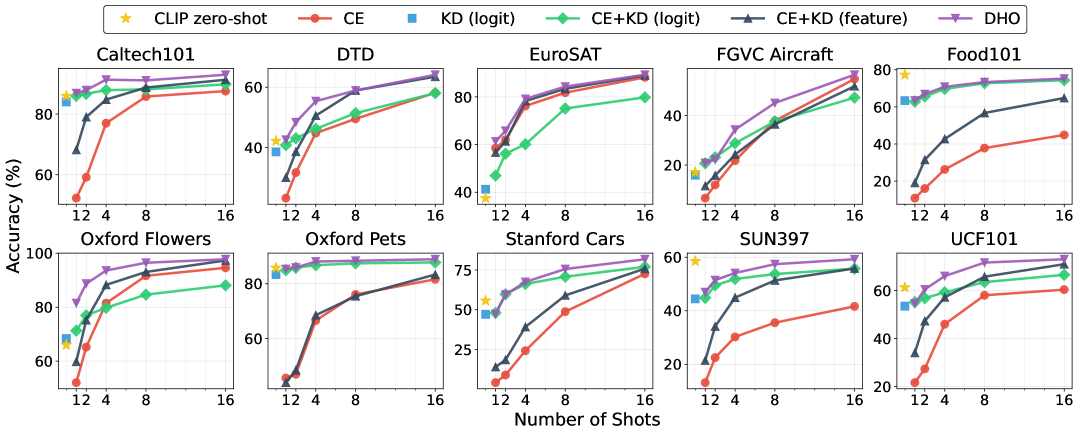
Figure 11: Results on 10 datasets under few-shot semi-supervision using MobileNetV2 with zero-shot teacher Radford et al. [2021].

Figure 12: Results on 10 datasets using MobileNetV2 with either zero- or few-shot teacher Zhang et al. [2021].

To demonstrate the versatility of our DHO approach beyond ResNet He et al. [2016] and ViT Dosovitskiy [2020] architectures, we extended our experiments to the MobileNetV2 Sandler et al. [2018], which is specifically designed for real-world applications with compact models. We maintained identical experimental settings as described in Section˜B.2, using MobileNetV2 as the student model while distilling from CLIP ResNet50.

As illustrated in Figure˜12, our DHO consistently outperforms all single-head baseline methods, demonstrating its effectiveness on lightweight model architectures along with ResNet18. Furthermore, Figure˜12 reveals patterns similar to our ResNet18 experiments regarding few-shot integration. Our method successfully incorporates few-shot teacher knowledge, although we observe that the few-shot teacher does not consistently yield improvements over the zero-shot teacher. Notably, our distilled MobileNetV2 model sometimes achieves superior performance to the few-shot teacher (ResNet-50) despite having significantly fewer parameters.

D.2 Out-of-Distribution Generalization

While our DHO framework is primarily designed for task-specific adaptation, we extensively evaluate its generalization capabilities across distribution-shifted scenarios. We conduct comprehensive experiments on four widely-used distribution-shifted variants of ImageNet: ImageNet-v2 Recht et al. [2019], ImageNet-Sketch Wang et al. [2019], ImageNet-R Hendrycks et al. [2021a], and ImageNet-A Hendrycks et al. [2021b] (detailed dataset characteristics are presented in Table˜10).

Table 11: Implementation details for our out-of-distribution generalization experiments.

Full Training
Model Configuration	Training Details
• Student: CLIP ViT-B/16 Radford et al. [2021] • Student input size: 224$\times$224 • Zero-shot Teacher: CLIP ViT-L/14 Radford et al. [2021] • Teacher input size: 336$\times$336 • Labeled data: 1% and 10% ImageNet • $\zeta$, $\eta$, and $\lambda$: $0.01,2,0.5$ • $\alpha$ and $\beta$: $0.5$ and $1$	• Epochs: 32 • Optimizer: AdamW ($\beta_{1}$=0.9, $\beta_{2}$=0.999) • Learning rate: $5\times 10^{-5}$, weight decay: $5\times 10^{-2}$ • Batch size: 512 (labeled: 256, unlabeled: 256) • Scheduler: Cosine warmup decay (5000 steps) • Augmentation: Random crops (x0.5-1.0), horizontal flips
Adaptation Methods (Linear Evaluation & Visual Prompt Tuning)
Method Configuration	Training Details
• Linear evaluation Caron et al. [2021] • Visual prompt tuning Jia et al. [2022] • Frozen backbone: CLIP ViT-B/16 Radford et al. [2021] • Input size: 224$\times$224 • Zero-shot Teacher: CLIP ViT-L/14 Radford et al. [2021] • Teacher input size: 336$\times$336 • Labeled data: 1% and 10% ImageNet • $\zeta$, $\eta$, and $\lambda$: $0.01,2,0.5$ • $\alpha$ and $\beta$: $0.5$ and $1$	• Epochs: 20 • Optimizer: AdamW ($\beta_{1}$=0.9, $\beta_{2}$=0.999) • Learning rate: $5\times 10^{-5}$, weight decay: $5\times 10^{-2}$ • Batch size: 512 (labeled: 256, unlabeled: 256) • Scheduler: Cosine warmup decay (5000 steps) • Augmentation: Random crops (x0.5-1.0), horizontal flips
Adaptation Methods (Prompt Tuning)
Method Configuration	Training Details
• Prompt tuning: CoOp Zhou et al. [2022b], PromptSRC Khattak et al. [2023b] • Frozen backbone: CLIP ViT-B/16 Radford et al. [2021] • Input size: 224$\times$224 • Zero-shot Teacher: CLIP ViT-L/14 Radford et al. [2021] • Teacher input size: 336$\times$336 • Labeled data: 1% and 10% ImageNet • $\zeta$, $\eta$, and $\lambda$: $0.01,2,0.5$ • $\alpha$ and $\beta$: $0.5$ and $1$	• Prompt tuning: Following PromptSRC Khattak et al. [2023b] configurations • Comparison: CasPL Wu et al. [2025] with domain-specific unlabeled data

Our analysis consists of two main components. First, we directly evaluate our ImageNet semi-supervised models on these distribution-shifted benchmarks to assess how DHO impacts robustness. Second, we investigate the integration of established adaptation techniques while preserving generalization capabilities. Our investigation begins with linear evaluation protocols Radford et al. [2021] and Visual Prompt Tuning Jia et al. [2022] using frozen image backbones. We then extend our analysis to state-of-the-art CLIP-based few-shot adaptation methods, specifically examining CoOp Zhou et al. [2022b] for unimodal prompt tuning and PromptSRC Khattak et al. [2023b] for multimodal prompt tuning approaches. Additionally, we compare our framework with CasPL Wu et al. [2025], which leverages domain-specific unlabeled data with separate distillation stage to enhance adaptation performance.

To evaluate our approach’s effectiveness under different data availability scenarios, we conducted experiments under both 1% and 10% labeled data settings, maintaining balanced loss weights of 0.5-0.5 and fixed values of $\alpha=0.5$ and $\beta=1.0$ for inference. Throughout the training process, we ensured consistent conditions by maintaining a 1:1 ratio of labeled to unlabeled samples in the batch composition. For experiments utilizing only labeled samples, we matched the number of training steps to those experiments using both labeled and unlabeled data to ensure fair comparison.

Evaluation upon Full Training Model.

Table 12: Accuracy(%) of DHO with full training model on the ImageNet distribution-shifted variants.

Student Model	Params (M)	Labeled Data	Teacher Model	Val	V2	Sketch	R	A
ViT-B/16 Student
ViT-B/16 Radford et al. [2021]	86M	zero-shot	-	66.7	60.8	46.2	74.0	47.0
ViT-B/16	86M	1%	ViT-L/14	78.7	70.1	48.0	70.9	41.1
ViT-B/16	86M	10%	ViT-L/14	80.8	71.3	47.4	71.7	41.4
ViT-B/16	86M	1%	ViT-H/14	81.6	72.6	50.6	65.5	35.6
ViT-B/16	86M	10%	ViT-H/14	82.8	73.6	50.7	67.7	37.8
ViT-L/14 Student
ViT-L/14 Radford et al. [2021]	304M	zero-shot	-	75.3	68.3	59.2	86.5	74.6
ViT-L/14	304M	1%	ViT-H/14	84.6	77.0	61.5	79.9	60.8
ViT-L/14	304M	10%	ViT-H/14	85.9	77.8	61.7	82.8	64.4
Zero-shot VLM
ViT-H Fang et al. [2023]	632M	zero-shot	-	83.6	77.2	71.7	92.3	77.4

DHO significantly outperformed zero-shot baselines on similar-distribution ImageNet variants (Table˜12), demonstrating particularly strong performance on ImageNet-V2 while maintaining reasonable accuracy on ImageNet-Sketch. This performance pattern remained consistent across both ViT-B/16 and ViT-L/14 architectures, with our approach showing improvements on similar-distribution test sets. However, when evaluated on out-of-distribution datasets such as ImageNet-R and ImageNet-A, the model exhibited performance degradation compared to zero-shot predictions, suggesting that full model training led to increased distribution overfitting and compromised generalization capability across domains.

A particularly insightful observation emerged from our analysis of different teacher-student configurations. Interestingly, ViT-B/16 models distilled from ViT-L/14 handled shifted distributions better than those taught by the larger ViT-H/14 DFN Fang et al. [2023], despite the latter’s superior performance on shifted distributions such as ImageNet-R and ImageNet-A. We attribute this to the shared training background between ViT-B/16 and ViT-L/14 in the CLIP framework Radford et al. [2021], which appears to better preserve generalization capabilities during the adaptation. This points to an important insight: our method works best on out-of-distributions when the teacher and student models share similar training distributions, suggesting that successful knowledge distillation also depends on the alignment between teacher and student than just the teacher’s raw capabilities.

Evaluation upon Adaptation Methods.

Table 13: Accuracy(%) of DHO with adaptation methods on the ImageNet distribution-shifted variants. $\dagger$: backbone frozen during training. VPT-$n$ indicates Visual Prompt Tuning with prompt depth of $n$ layers. For fair comparison, we used $\alpha=0.5$ and $\beta=1.0$ for all DHO evaluation.

Method	Labeled	Teacher	Unlabeled	Val	V2	Sketch	R	A
	Data	Model	Data
CLIP Zero-shot
CLIP Radford et al. [2021]	-	-	-	66.7	60.8	46.2	74.0	47.8
Linear Evaluation
Linear Evaluation	1%	-	-	72.8	64.2	47.0	74.6	48.6
DHO†	1%	✓	-	73.4	65.3	48.3	75.8	49.4
DHO†	1%	✓	✓	74.6	66.4	49.2	76.1	49.8
Visual Prompt Tuning
VPT-3 Jia et al. [2022]	1.25%	-	-	73.6	64.6	47.7	75.2	48.7
VPT-3+DHO	1.25%	✓	-	73.6	65.3	48.7	75.9	49.1
VPT-3+DHO	1.25%	✓	✓	75.1	66.8	50.0	76.9	50.5
VPT-9+DHO	1.25%	✓	-	74.0	65.9	48.9	75.8	46.5
VPT-9+DHO	1.25%	✓	✓	75.6	67.4	50.8	77.3	46.5
VLM Text-encoder Prompt Tuning
CoOp Zhou et al. [2022b]	1.25% (16-shots)	-	-	71.5	64.2	48.0	75.2	49.7
CoOp+CasPL Wu et al. [2025]	1.25% (16-shots)	✓	✓	71.9	64.3	48.3	76.0	-
CoOp+DHO	1.25% (16-shots)	✓	-	72.8	65.5	49.3	76.4	49.5
CoOp+DHO	1.25% (16-shots)	✓	✓	73.4	66.2	49.5	77.0	50.5
VLM Multimodal Prompt Tuning
PromptSRC Khattak et al. [2023b]	1.25% (16-shots)	-	-	71.3	64.4	49.6	77.8	50.9
PromptSRC+CasPL Wu et al. [2025]	1.25% (16-shots)	✓	✓	72.8	65.7	49.7	77.9	-
PromptSRC+DHO	1.25% (16-shots)	✓	-	73.0	65.3	49.5	77.8	51.3
PromptSRC+DHO	1.25% (16-shots)	✓	✓	73.6	66.1	49.8	78.1	51.0

As demonstrated in Table˜13, we first evaluated DHO in scenarios where only the image encoder is utilized: linear evaluation Radford et al. [2021] and visual prompt tuning Jia et al. [2022] with a frozen CLIP ViT-B/16 encoder. Notably, we discovered that linear evaluation with language initialization, as proposed in Li et al. [2022], performs remarkably well, even outperforming prompt tuning-based methods such as CoOp Zhou et al. [2022b] and PromptSRC Khattak et al. [2023b] on in-domain distribution benchmarks. With the additional pathway for teacher knowledge distillation, DHO achieves substantial performance improvements across all in-distribution and out-of-distribution evaluations, even with just 1% of labeled data. Furthermore, leveraging unlabeled data yields additional performance gains.

In experiments with visual prompt tuning, similar to our linear probing experiments, introducing a new optimization pathway for distillation resulted in performance improvements across all evaluation benchmarks, with further enhancements when utilizing unlabeled data. Moreover, increasing the number of learnable parameters by adding prompt layers led to improved performance across all datasets, with ImageNet-A being the sole exception.

We also evaluated DHO on various VLM adaptation methods, including the text-encoder prompt learning approach CoOp Zhou et al. [2022b], the multi-modal prompt learning method PromptSRC Khattak et al. [2023b], and the recently proposed CasPL Wu et al. [2025], which employs a teacher network for unsupervised distillation on unlabeled data as a separate stage. We used the same implementation from the domain generalization setting of the original papers Zhou et al. [2022b], Khattak et al. [2023b], with only a linear layer jointly trained on top of image encoder features as the distillation pathway.

Our results demonstrate that the simple integration of DHO with existing approaches yields remarkable outcomes as shown in Table˜13, achieving average improvements of 0.9% and 0.3% across four generalization benchmarks upon CoOp and PromptSRC, respectively. Notably, when compared to CasPL, which utilizes a teacher network with domain unlabeled datasets, our DHO approach demonstrates superior performance across all in-distribution and out-of-distribution benchmarks, achieving new state-of-the-art results when leveraging both teacher and unlabeled domain datasets. This suggests that joint training of labeled supervision and teacher distillation signals is a more effective strategy than the sequential approach used in CasPL, aligning with our core hypothesis about the benefits of dual-head optimization for resolving gradient conflicts.

Appendix E Additional Analysis

E.1 Gradient Analysis

Figure 13: (Left): The average dominant eigenvalue $\lambda$ of $WW^{\top}$ and $W_{\text{CE}}W_{\text{KD}}^{\top}$ during training. (Right): The average cosine similarity of gradients w.r.t features $\mathtt{CosSim}(\nabla_{z}\mathcal{L}_{\text{CE}},\nabla_{z}\mathcal{L}_{\text{KD}})$.

We analyze the gradient conflict occurs in one of single-head KD baselines, logit distillation in §3.2. In this section, we present the dominant eigen value of $WW^{\top}$ and $W_{\text{CE}}W_{\text{KD}}$ during training in Figure˜13-(Left). We further present the cosine similarity between gradients w.r.t feature representation $z$ in Figure˜13-(Right). The trend of cosine similarity between feature gradients is similar to that of full gradients $\mathtt{CosSim}(\nabla_{\theta}\mathcal{L}_{\text{CE}},\nabla_{\theta}\mathcal{L}_{\text{KD}})$ in Figure˜4.

E.2 Additional Analysis on Non-Linear Head Design

To further investigate the architectural advantages of dual head optimization, we conducted experiments with non-linear head designs, replacing the linear heads used in our main experiments. The non-linear classifier enhanced model representational capacity through a sequence of layers: an initial linear projection layer, followed by layer normalization Ba [2016], GELU activation Hendrycks and Gimpel [2016], dropout Srivastava et al. [2014], and a final linear classification layer. We compared DHO with three non-linear configurations; DHO+NL-Head-CE: non-linear CE head, DHO+NL-Head-KD: non-linear KD head, and DHO+NL-Head-CE+KD: non-linear both CE and KD heads. All experiments followed the few-shot semi-supervised setting detailed in Section˜B.2.

Figure 14: Results of different non-linear head configurations on 11 datasets including ImageNet under few-shot semi-supervision using ResNet-18 with zero-shot teacher Radford et al. [2021].

Table 14: Results of different non-linear head configurations on 11 datasets including ImageNet under few-shot semi-supervision using ResNet-18 with zero-shot teacher Radford et al. [2021]. We report averaged accuracy for 10 visual recognition datasets except the ImageNet.

	ImageNet						Average of 10 tasks
Configuration	1-shot	2-shot	4-shot	8-shot	16-shot		1-shot	2-shot	4-shot	8-shot	16-shot
DHO (base)	61.7	62.2	62.6	63.8	65.1		58.9	62.2	68.4	73.1	76.5
DHO+NL-Head-CE	61.7	61.9	62.2	63.1	64.8		59.3	62.1	68.0	72.7	76.2
DHO+NL-Head-KD	62.1	62.6	62.9	64.0	65.9		58.3	62.1	67.8	72.4	76.5
DHO+NL-Head-CE+KD	62.0	62.3	62.6	63.8	65.4		59.1	62.2	68.6	72.4	76.5

Table 15: Results on dual-heads interpolation strategy of different non-linear head configurations on ImageNet under 16-shots semi-supervised setting.

Configuration	CE Head	KD Head	Combined
DHO (base)	60.64	61.55	65.37
DHO+NL-Head-CE	60.18	61.39	64.91
DHO+NL-Head-KD	60.95	61.76	65.97
DHO+NL-Head-CE+KD	61.66	61.81	65.59

Performance Analysis.

Our experiments on ImageNet revealed several key findings regarding head architecture (Table˜14, Figure˜14). Non-linear architectures in the KD head consistently improved performance compared to the linear approach, suggesting that complex architectures better capture teacher predictions. However, increasing complexity in the CE head resulted in performance degradation, most likely due to this head’s focus on limited labeled data, which impaired its capacity to learn generalizable shared feature representations. While dual non-linear heads outperformed their fully linear counterparts, this configuration was less effective than implementing non-linearity solely in the KD head.

When extending our analysis to the other 10 datasets (Table˜14, Figure˜14), we observed a different pattern. Unlike on ImageNet, the optimal architectural configuration varied considerably across these diverse datasets, with no single configuration emerging as consistently superior. This contrast highlights that the effectiveness of non-linear transformations exhibits strong dataset-specific dependencies and varies according to head functionality. Given these findings, we adopted the linear head architecture for all subsequent experiments, as it achieved comparable performance while providing substantial benefits in computational efficiency and architectural simplicity.

Head Decomposition Analysis.

Our analysis under the 16-shot semi-supervised setting revealed intricate relationships between architectural choices and head-wise performance. When employing a non-linear CE branch, we observed a decline in CE head performance from $60.64\%$ to $60.18\%$, despite increased parameters. Conversely, implementing a non-linear architecture for the KD head improved both heads’ performance: CE head accuracy increased from $60.64\%$ to $60.95\%$, and KD head prediction improved from $61.55\%$ to $61.76\%$. However, when applying non-linear architectures to both heads simultaneously, despite enhanced individual performance, the combined performance decreased from $65.97\%$ to $65.59\%$, suggesting that head specialization may compromise joint feature representation quality. These findings underscore the complex interplay between architectural decisions and multi-head learning dynamics in semi-supervised frameworks.

E.3 Additional Dual-Head Analysis

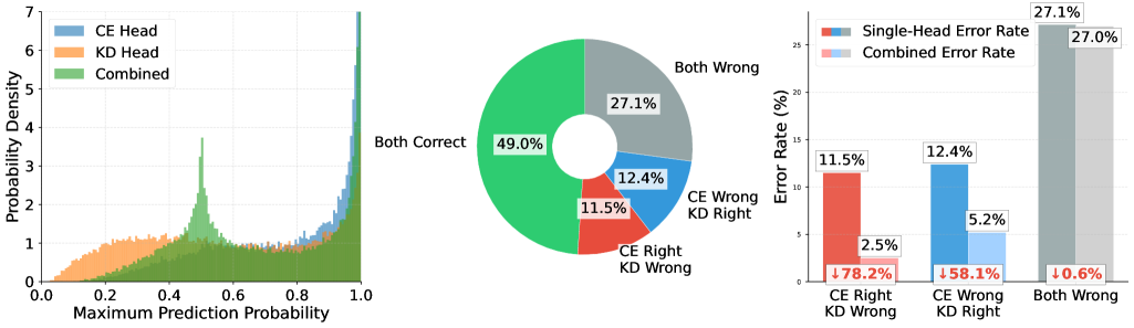
Figure 15: Analysis of DHO on the ImageNet under 16-shot semi-supervised setting. (Left) Maximum probability distributions for predictions from CE head, KD head, and their combined output. (Middle) Prediction agreement diagram analysis, categorizing cases where both heads are correct, only one head is correct, and both heads are incorrect. (Right) Error reduction analysis comparing single-head failure cases against improvements achieved through combined predictions.

In this section, we further analyze the prediction behavior of DHO. As shown in Figure˜15 (left), despite sharing feature representations, the CE head ($h_{\text{CE}}$), trained on labeled data, produces sharper predictions, whereas the KD head ($h_{\text{KD}}$), guided by teacher distillation, generates smoother distributions. Prediction agreement analysis (Figure˜15, middle) shows that the two heads agree in 76.2% of cases while complementing each other: the CE head correctly classifies 11.5% of cases where the KD head fails, and vice versa for 12.4%. Error reduction analysis (Figure˜15, right) further demonstrates that our combined approach reduces failure rates from 11.5% to 2.5% for the KD head and from 12.4% to 5.2% for the CE head, confirming the effectiveness of DHO.

We also present additional qualitative results of DHO, both on ImageNet (see Figures˜16 and 17) and on other 10 datasets (see Figures˜18 and 19).

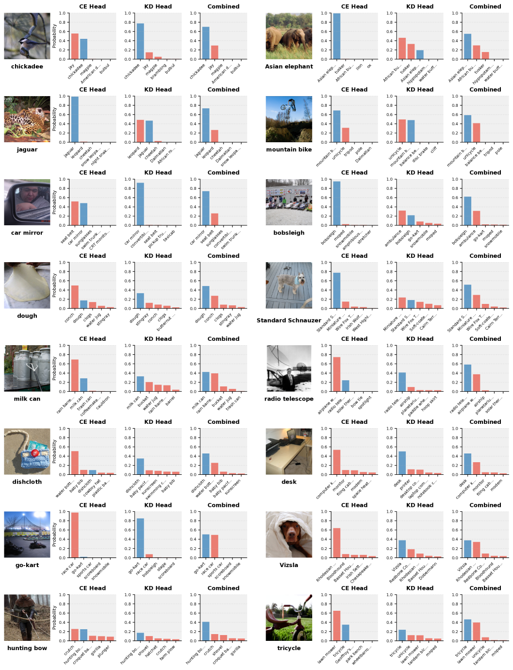
Figure 16: Additional qualitative results on ImageNet under 16-shot semi-supervised setting.

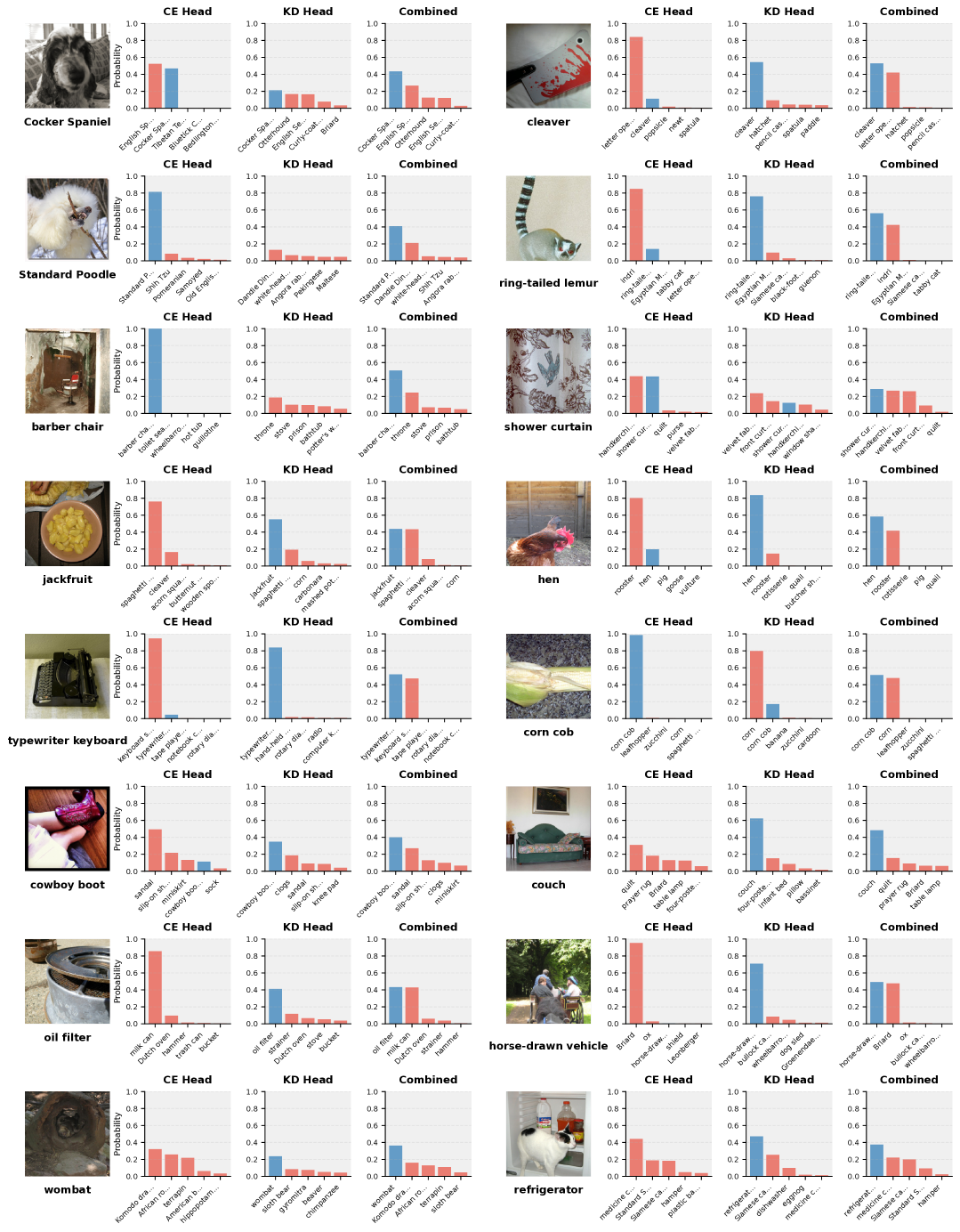
Figure 17: Additional qualitative results on ImageNet under 16-shot semi-supervised setting.

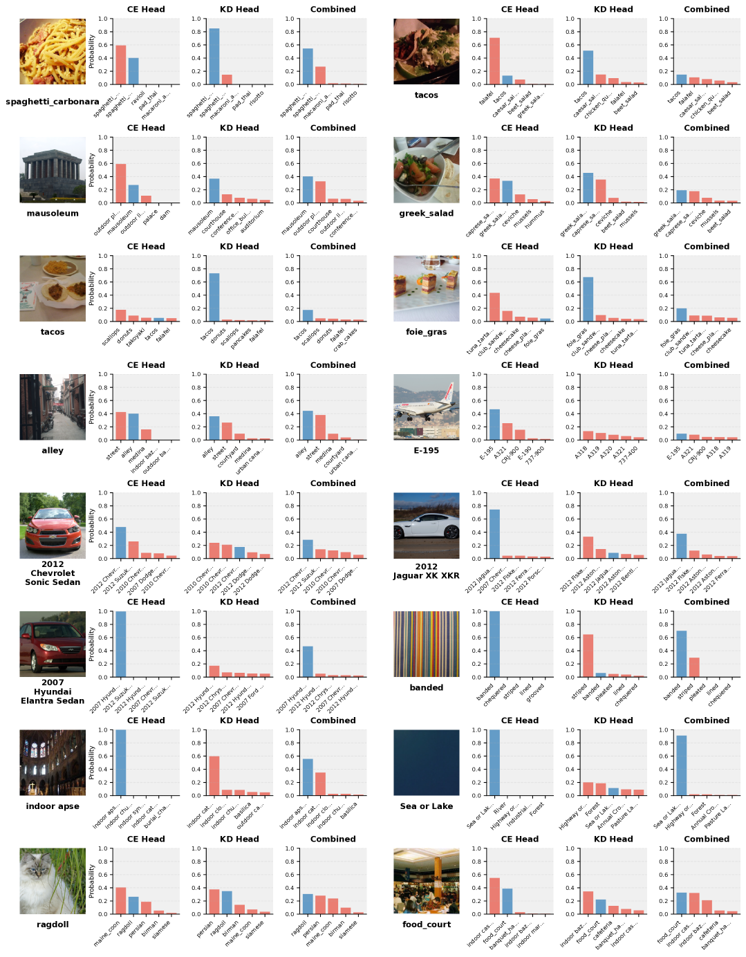
Figure 18: Additional qualitative results 1 on other 10 datasets of model trained under 16-shot semi-supervised setting

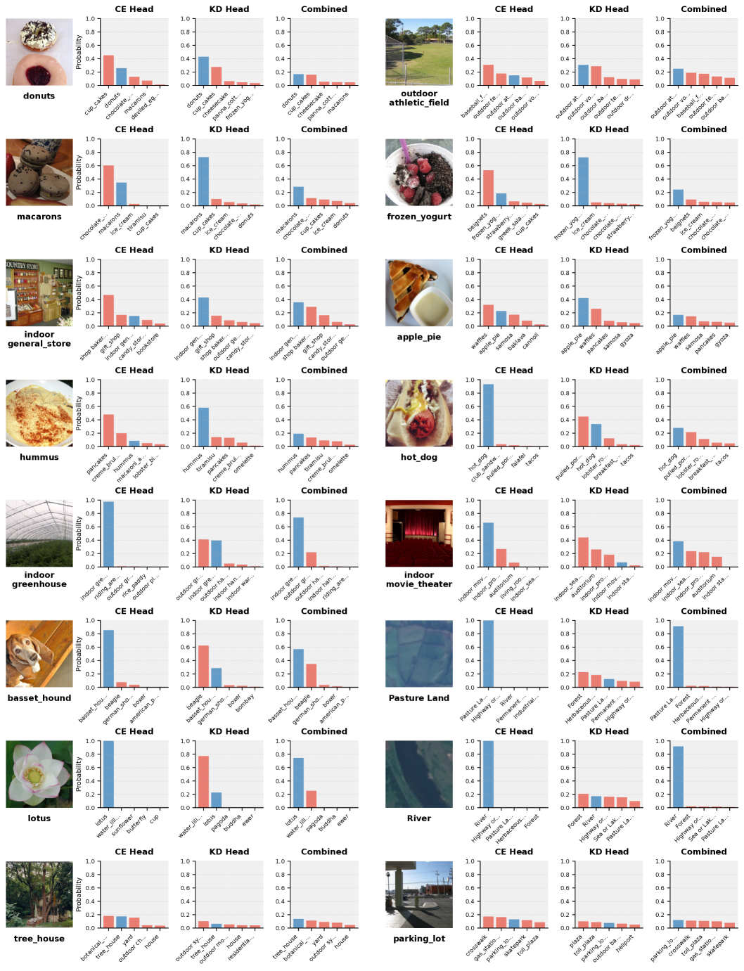
Figure 19: Additional qualitative results 2 on other 10 datasets of model trained under 16-shot semi-supervised setting

NeurIPS Paper Checklist

1. Claims

2. Question: Do the main claims made in the abstract and introduction accurately reflect the paper’s contributions and scope?

3. Answer: [Yes]

4. Justification: Yes. Our main contributions are also detailed in §1. Our gradient conflict analysis is presented in §3.2 and Section˜E.1. We also provide post-hoc analysis on dual-head combination in Appendix˜A with empirical analysis in Section˜E.3.

5. Guidelines:

   • The answer NA means that the abstract and introduction do not include the claims made in the paper.

   • The abstract and/or introduction should clearly state the claims made, including the contributions made in the paper and important assumptions and limitations. A No or NA answer to this question will not be perceived well by the reviewers.

   • The claims made should match theoretical and experimental results, and reflect how much the results can be expected to generalize to other settings.

   • It is fine to include aspirational goals as motivation as long as it is clear that these goals are not attained by the paper.

6. Limitations

7. Question: Does the paper discuss the limitations of the work performed by the authors?

8. Answer: [Yes]

9. Justification: Yes, we discussed limitations in §5. We also reported computational cost in training in Section˜B.2, and analyzed the computational efficiency of our method in §4.2 (Table˜2) and Section˜B.3.

10. Guidelines:

    • The answer NA means that the paper has no limitation while the answer No means that the paper has limitations, but those are not discussed in the paper.

    • The authors are encouraged to create a separate "Limitations" section in their paper.

    • The paper should point out any strong assumptions and how robust the results are to violations of these assumptions (e.g., independence assumptions, noiseless settings, model well-specification, asymptotic approximations only holding locally). The authors should reflect on how these assumptions might be violated in practice and what the implications would be.

    • The authors should reflect on the scope of the claims made, e.g., if the approach was only tested on a few datasets or with a few runs. In general, empirical results often depend on implicit assumptions, which should be articulated.

    • The authors should reflect on the factors that influence the performance of the approach. For example, a facial recognition algorithm may perform poorly when image resolution is low or images are taken in low lighting. Or a speech-to-text system might not be used reliably to provide closed captions for online lectures because it fails to handle technical jargon.

    • The authors should discuss the computational efficiency of the proposed algorithms and how they scale with dataset size.

    • If applicable, the authors should discuss possible limitations of their approach to address problems of privacy and fairness.

    • While the authors might fear that complete honesty about limitations might be used by reviewers as grounds for rejection, a worse outcome might be that reviewers discover limitations that aren’t acknowledged in the paper. The authors should use their best judgment and recognize that individual actions in favor of transparency play an important role in developing norms that preserve the integrity of the community. Reviewers will be specifically instructed to not penalize honesty concerning limitations.

11. Theory assumptions and proofs

12. Question: For each theoretical result, does the paper provide the full set of assumptions and a complete (and correct) proof?

13. Answer: [Yes]

14. Justification: Yes, we provided the full set of assumptions and a complete (and correct) proof for gradient conflict analysis and post-hoc dual-head balancing in §3.2 and §A, respectively.

15. Guidelines:

    • The answer NA means that the paper does not include theoretical results.

    • All the theorems, formulas, and proofs in the paper should be numbered and cross-referenced.

    • All assumptions should be clearly stated or referenced in the statement of any theorems.

    • The proofs can either appear in the main paper or the supplemental material, but if they appear in the supplemental material, the authors are encouraged to provide a short proof sketch to provide intuition.

    • Inversely, any informal proof provided in the core of the paper should be complemented by formal proofs provided in appendix or supplemental material.

    • Theorems and Lemmas that the proof relies upon should be properly referenced.

16. Experimental result reproducibility

17. Question: Does the paper fully disclose all the information needed to reproduce the main experimental results of the paper to the extent that it affects the main claims and/or conclusions of the paper (regardless of whether the code and data are provided or not)?

18. Answer: [Yes]

19. Justification: We used publicly available datasets and models for our experiments. Our proposed method is also simple and easy to implement, with described details in §4. We will also release our code and instructions for reproducing the results.

20. Guidelines:

    • The answer NA means that the paper does not include experiments.

    • If the paper includes experiments, a No answer to this question will not be perceived well by the reviewers: Making the paper reproducible is important, regardless of whether the code and data are provided or not.

    • If the contribution is a dataset and/or model, the authors should describe the steps taken to make their results reproducible or verifiable.

    • Depending on the contribution, reproducibility can be accomplished in various ways. For example, if the contribution is a novel architecture, describing the architecture fully might suffice, or if the contribution is a specific model and empirical evaluation, it may be necessary to either make it possible for others to replicate the model with the same dataset, or provide access to the model. In general. releasing code and data is often one good way to accomplish this, but reproducibility can also be provided via detailed instructions for how to replicate the results, access to a hosted model (e.g., in the case of a large language model), releasing of a model checkpoint, or other means that are appropriate to the research performed.

    • While NeurIPS does not require releasing code, the conference does require all submissions to provide some reasonable avenue for reproducibility, which may depend on the nature of the contribution. For example

      1. If the contribution is primarily a new algorithm, the paper should make it clear how to reproduce that algorithm.

      2. If the contribution is primarily a new model architecture, the paper should describe the architecture clearly and fully.

      3. If the contribution is a new model (e.g., a large language model), then there should either be a way to access this model for reproducing the results or a way to reproduce the model (e.g., with an open-source dataset or instructions for how to construct the dataset).

      4. We recognize that reproducibility may be tricky in some cases, in which case authors are welcome to describe the particular way they provide for reproducibility. In the case of closed-source models, it may be that access to the model is limited in some way (e.g., to registered users), but it should be possible for other researchers to have some path to reproducing or verifying the results.

21. Open access to data and code

22. Question: Does the paper provide open access to the data and code, with sufficient instructions to faithfully reproduce the main experimental results, as described in supplemental material?

23. Answer: [Yes]

24. Justification: We will provide open access to the data and code, with sufficient instructions to faithfully reproduce the main experimental results, once the blind review is over.

25. Guidelines:

    • The answer NA means that paper does not include experiments requiring code.

    • Please see the NeurIPS code and data submission guidelines (https://nips.cc/public/guides/CodeSubmissionPolicy) for more details.

    • While we encourage the release of code and data, we understand that this might not be possible, so "No" is an acceptable answer. Papers cannot be rejected simply for not including code, unless this is central to the contribution (e.g., for a new open-source benchmark).

    • The instructions should contain the exact command and environment needed to run to reproduce the results. See the NeurIPS code and data submission guidelines (https://nips.cc/public/guides/CodeSubmissionPolicy) for more details.

    • The authors should provide instructions on data access and preparation, including how to access the raw data, preprocessed data, intermediate data, and generated data, etc.

    • The authors should provide scripts to reproduce all experimental results for the new proposed method and baselines. If only a subset of experiments are reproducible, they should state which ones are omitted from the script and why.

    • At submission time, to preserve anonymity, the authors should release anonymized versions (if applicable).

    • Providing as much information as possible in supplemental material (appended to the paper) is recommended, but including URLs to data and code is permitted.

26. Experimental setting/details

27. Question: Does the paper specify all the training and test details (e.g., data splits, hyperparameters, how they were chosen, type of optimizer, etc.) necessary to understand the results?

28. Answer: [Yes]

29. Justification: We specified all the training and test details (e.g., data splits, hyperparameters, how they were chosen, type of optimizer, etc.) necessary to understand the results in §4.1 and Section˜B.2.

30. Guidelines:

    • The answer NA means that the paper does not include experiments.

    • The experimental setting should be presented in the core of the paper to a level of detail that is necessary to appreciate the results and make sense of them.

    • The full details can be provided either with the code, in appendix, or as supplemental material.

31. Experiment statistical significance

32. Question: Does the paper report error bars suitably and correctly defined or other appropriate information about the statistical significance of the experiments?

33. Answer: [No]

34. Justification: We couldn’t report error bars due to computational resource constraints, as described in Table˜8 in Section˜B.2. Our experiments cover a variety of few-shot settings (1, 2, 4, 8, 16 shots) across multiple datasets (11 datasets including ImageNet), making multiple runs prohibitively expensive. However, our work demonstrates consistent performance gaps compared to baselines across all experimental settings, providing strong evidence for the effectiveness of our approach.

35. Guidelines:

    • The answer NA means that the paper does not include experiments.

    • The authors should answer "Yes" if the results are accompanied by error bars, confidence intervals, or statistical significance tests, at least for the experiments that support the main claims of the paper.

    • The factors of variability that the error bars are capturing should be clearly stated (for example, train/test split, initialization, random drawing of some parameter, or overall run with given experimental conditions).

    • The method for calculating the error bars should be explained (closed form formula, call to a library function, bootstrap, etc.)

    • The assumptions made should be given (e.g., Normally distributed errors).

    • It should be clear whether the error bar is the standard deviation or the standard error of the mean.

    • It is OK to report 1-sigma error bars, but one should state it. The authors should preferably report a 2-sigma error bar than state that they have a 96% CI, if the hypothesis of Normality of errors is not verified.

    • For asymmetric distributions, the authors should be careful not to show in tables or figures symmetric error bars that would yield results that are out of range (e.g. negative error rates).

    • If error bars are reported in tables or plots, The authors should explain in the text how they were calculated and reference the corresponding figures or tables in the text.

36. Experiments compute resources

37. Question: For each experiment, does the paper provide sufficient information on the computer resources (type of compute workers, memory, time of execution) needed to reproduce the experiments?

38. Answer: [Yes]

39. Justification: We provided type of hardware, and time of execution needed to reproduce the experiments in Table˜8 inside Section˜B.2 for experiments taking the most time. Also we provided extensive information of computational efficiency of our method in §4.2 and Section˜B.3.

40. Guidelines:

    • The answer NA means that the paper does not include experiments.

    • The paper should indicate the type of compute workers CPU or GPU, internal cluster, or cloud provider, including relevant memory and storage.

    • The paper should provide the amount of compute required for each of the individual experimental runs as well as estimate the total compute.

    • The paper should disclose whether the full research project required more compute than the experiments reported in the paper (e.g., preliminary or failed experiments that didn’t make it into the paper).

41. Code of ethics

42. Question: Does the research conducted in the paper conform, in every respect, with the NeurIPS Code of Ethics https://neurips.cc/public/EthicsGuidelines?

43. Answer: [Yes]

44. Justification: Yes, we followed the NeurIPS Code of Ethics https://neurips.cc/public/EthicsGuidelines.

45. Guidelines:

    • The answer NA means that the authors have not reviewed the NeurIPS Code of Ethics.

    • If the authors answer No, they should explain the special circumstances that require a deviation from the Code of Ethics.

    • The authors should make sure to preserve anonymity (e.g., if there is a special consideration due to laws or regulations in their jurisdiction).

46. Broader impacts

47. Question: Does the paper discuss both potential positive societal impacts and negative societal impacts of the work performed?

48. Answer: [N/A]

49. Justification: Our work uses only standard academic datasets like ImageNet for improving semi-supervised learning methods. We don’t use any private or personal data, and our techniques don’t present obvious negative societal impacts.

50. Guidelines:

    • The answer NA means that there is no societal impact of the work performed.

    • If the authors answer NA or No, they should explain why their work has no societal impact or why the paper does not address societal impact.

    • Examples of negative societal impacts include potential malicious or unintended uses (e.g., disinformation, generating fake profiles, surveillance), fairness considerations (e.g., deployment of technologies that could make decisions that unfairly impact specific groups), privacy considerations, and security considerations.

    • The conference expects that many papers will be foundational research and not tied to particular applications, let alone deployments. However, if there is a direct path to any negative applications, the authors should point it out. For example, it is legitimate to point out that an improvement in the quality of generative models could be used to generate deepfakes for disinformation. On the other hand, it is not needed to point out that a generic algorithm for optimizing neural networks could enable people to train models that generate Deepfakes faster.

    • The authors should consider possible harms that could arise when the technology is being used as intended and functioning correctly, harms that could arise when the technology is being used as intended but gives incorrect results, and harms following from (intentional or unintentional) misuse of the technology.

    • If there are negative societal impacts, the authors could also discuss possible mitigation strategies (e.g., gated release of models, providing defenses in addition to attacks, mechanisms for monitoring misuse, mechanisms to monitor how a system learns from feedback over time, improving the efficiency and accessibility of ML).

51. Safeguards

52. Question: Does the paper describe safeguards that have been put in place for responsible release of data or models that have a high risk for misuse (e.g., pretrained language models, image generators, or scraped datasets)?

53. Answer: [N/A]

54. Justification: Our work focuses on semi-supervised learning methods using standard academic datasets and does not pose high risks for misuse.

55. Guidelines:

    • The answer NA means that the paper poses no such risks.

    • Released models that have a high risk for misuse or dual-use should be released with necessary safeguards to allow for controlled use of the model, for example by requiring that users adhere to usage guidelines or restrictions to access the model or implementing safety filters.

    • Datasets that have been scraped from the Internet could pose safety risks. The authors should describe how they avoided releasing unsafe images.

    • We recognize that providing effective safeguards is challenging, and many papers do not require this, but we encourage authors to take this into account and make a best faith effort.

56. Licenses for existing assets

57. Question: Are the creators or original owners of assets (e.g., code, data, models), used in the paper, properly credited and are the license and terms of use explicitly mentioned and properly respected?

58. Answer: [Yes]

59. Justification: We properly credit all creators of assets used in our work.

60. Guidelines:

    • The answer NA means that the paper does not use existing assets.

    • The authors should cite the original paper that produced the code package or dataset.

    • The authors should state which version of the asset is used and, if possible, include a URL.

    • The name of the license (e.g., CC-BY 4.0) should be included for each asset.

    • For scraped data from a particular source (e.g., website), the copyright and terms of service of that source should be provided.

    • If assets are released, the license, copyright information, and terms of use in the package should be provided. For popular datasets, paperswithcode.com/datasets has curated licenses for some datasets. Their licensing guide can help determine the license of a dataset.

    • For existing datasets that are re-packaged, both the original license and the license of the derived asset (if it has changed) should be provided.

    • If this information is not available online, the authors are encouraged to reach out to the asset’s creators.

61. New assets

62. Question: Are new assets introduced in the paper well documented and is the documentation provided alongside the assets?

63. Answer: [N/A]

64. Justification: Our work does not release any new assets such as datasets, code, or models.

65. Guidelines:

    • The answer NA means that the paper does not release new assets.

    • Researchers should communicate the details of the dataset/code/model as part of their submissions via structured templates. This includes details about training, license, limitations, etc.

    • The paper should discuss whether and how consent was obtained from people whose asset is used.

    • At submission time, remember to anonymize your assets (if applicable). You can either create an anonymized URL or include an anonymized zip file.

66. Crowdsourcing and research with human subjects

67. Question: For crowdsourcing experiments and research with human subjects, does the paper include the full text of instructions given to participants and screenshots, if applicable, as well as details about compensation (if any)?

68. Answer: [N/A]

69. Justification: Our work does not involve crowdsourcing or research with human subjects.

70. Guidelines:

    • The answer NA means that the paper does not involve crowdsourcing nor research with human subjects.

    • Including this information in the supplemental material is fine, but if the main contribution of the paper involves human subjects, then as much detail as possible should be included in the main paper.

    • According to the NeurIPS Code of Ethics, workers involved in data collection, curation, or other labor should be paid at least the minimum wage in the country of the data collector.

71. Institutional review board (IRB) approvals or equivalent for research with human subjects

72. Question: Does the paper describe potential risks incurred by study participants, whether such risks were disclosed to the subjects, and whether Institutional Review Board (IRB) approvals (or an equivalent approval/review based on the requirements of your country or institution) were obtained?

73. Answer: [N/A]

74. Justification: Our work does not involve crowdsourcing or research with human subjects.

75. Guidelines:

    • The answer NA means that the paper does not involve crowdsourcing nor research with human subjects.

    • Depending on the country in which research is conducted, IRB approval (or equivalent) may be required for any human subjects research. If you obtained IRB approval, you should clearly state this in the paper.

    • We recognize that the procedures for this may vary significantly between institutions and locations, and we expect authors to adhere to the NeurIPS Code of Ethics and the guidelines for their institution.

    • For initial submissions, do not include any information that would break anonymity (if applicable), such as the institution conducting the review.

76. Declaration of LLM usage

77. Question: Does the paper describe the usage of LLMs if it is an important, original, or non-standard component of the core methods in this research? Note that if the LLM is used only for writing, editing, or formatting purposes and does not impact the core methodology, scientific rigorousness, or originality of the research, declaration is not required.

78. Answer: [N/A]

79. Justification: Our work does not involve any LLMs as important, original, or non-standard components.

80. Guidelines:

    • The answer NA means that the core method development in this research does not involve LLMs as any important, original, or non-standard components.

    • Please refer to our LLM policy (https://neurips.cc/Conferences/2025/LLM) for what should or should not be described.

References

- Abbasi Koohpayegani et al. [2020] Soroush Abbasi Koohpayegani, Ajinkya Tejankar, and Hamed Pirsiavash. Compress: Self-supervised learning by compressing representations. Advances in Neural Information Processing Systems, 33:12980–12992, 2020.
- Assran et al. [2021] Mahmoud Assran, Mathilde Caron, Ishan Misra, Piotr Bojanowski, Armand Joulin, Nicolas Ballas, and Michael Rabbat. Semi-supervised learning of visual features by non-parametrically predicting view assignments with support samples. In Proceedings of the IEEE/CVF International Conference on Computer Vision, pages 8443–8452, 2021.
- Assran et al. [2022] Mahmoud Assran, Mathilde Caron, Ishan Misra, Piotr Bojanowski, Florian Bordes, Pascal Vincent, Armand Joulin, Mike Rabbat, and Nicolas Ballas. Masked siamese networks for label-efficient learning. In European Conference on Computer Vision, pages 456–473. Springer, 2022.
- Ba [2016] Jimmy Lei Ba. Layer normalization. arXiv preprint arXiv:1607.06450, 2016.
- Bolya et al. [2022] Daniel Bolya, Cheng-Yang Fu, Xiaoliang Dai, Peizhao Zhang, Christoph Feichtenhofer, and Judy Hoffman. Token merging: Your vit but faster. arXiv preprint arXiv:2210.09461, 2022.
- Bossard et al. [2014] Lukas Bossard, Matthieu Guillaumin, and Luc Van Gool. Food-101–mining discriminative components with random forests. In Computer vision–ECCV 2014: 13th European conference, zurich, Switzerland, September 6-12, 2014, proceedings, part VI 13, pages 446–461. Springer, 2014.
- Cai et al. [2022] Zhaowei Cai, Avinash Ravichandran, Paolo Favaro, Manchen Wang, Davide Modolo, Rahul Bhotika, Zhuowen Tu, and Stefano Soatto. Semi-supervised vision transformers at scale. Advances in Neural Information Processing Systems, 35:25697–25710, 2022.
- Caron et al. [2021] Mathilde Caron, Hugo Touvron, Ishan Misra, Hervé Jégou, Julien Mairal, Piotr Bojanowski, and Armand Joulin. Emerging properties in self-supervised vision transformers. In Proceedings of the IEEE/CVF international conference on computer vision, pages 9650–9660, 2021.
- Chen et al. [2023] Fei-Long Chen, Du-Zhen Zhang, Ming-Lun Han, Xiu-Yi Chen, Jing Shi, Shuang Xu, and Bo Xu. Vlp: A survey on vision-language pre-training. Machine Intelligence Research, 20(1):38–56, 2023.
- Chen et al. [2019] Hanting Chen, Yunhe Wang, Chang Xu, Zhaohui Yang, Chuanjian Liu, Boxin Shi, Chunjing Xu, Chao Xu, and Qi Tian. Data-free learning of student networks. In Proceedings of the IEEE/CVF international conference on computer vision, pages 3514–3522, 2019.
- Chen and Er [2025] Jie Chen and Meng Joo Er. Mitigating gradient conflicts via expert squads in multi-task learning. Neurocomputing, 614:128832, 2025.
- Chen et al. [2020a] Ting Chen, Simon Kornblith, Mohammad Norouzi, and Geoffrey Hinton. A simple framework for contrastive learning of visual representations. In International conference on machine learning, pages 1597–1607. PMLR, 2020a.
- Chen et al. [2020b] Ting Chen, Simon Kornblith, Kevin Swersky, Mohammad Norouzi, and Geoffrey E Hinton. Big self-supervised models are strong semi-supervised learners. Advances in neural information processing systems, 33:22243–22255, 2020b.
- Chen et al. [2024] Yifan Chen, Xiaozhen Qiao, Zhe Sun, and Xuelong Li. Comkd-clip: Comprehensive knowledge distillation for contrastive language-image pre-traning model. arXiv preprint arXiv:2408.04145, 2024.
- Cherti et al. [2023] Mehdi Cherti, Romain Beaumont, Ross Wightman, Mitchell Wortsman, Gabriel Ilharco, Cade Gordon, Christoph Schuhmann, Ludwig Schmidt, and Jenia Jitsev. Reproducible scaling laws for contrastive language-image learning. In Proceedings of the IEEE/CVF Conference on Computer Vision and Pattern Recognition, pages 2818–2829, 2023.
- Cho and Hariharan [2019] Jang Hyun Cho and Bharath Hariharan. On the efficacy of knowledge distillation. In Proceedings of the IEEE/CVF international conference on computer vision, pages 4794–4802, 2019.
- Cimpoi et al. [2014] Mircea Cimpoi, Subhransu Maji, Iasonas Kokkinos, Sammy Mohamed, and Andrea Vedaldi. Describing textures in the wild. In Proceedings of the IEEE conference on computer vision and pattern recognition, pages 3606–3613, 2014.
- Dehghani et al. [2023] Mostafa Dehghani, Josip Djolonga, Basil Mustafa, Piotr Padlewski, Jonathan Heek, Justin Gilmer, Andreas Peter Steiner, Mathilde Caron, Robert Geirhos, Ibrahim Alabdulmohsin, et al. Scaling vision transformers to 22 billion parameters. In International Conference on Machine Learning, pages 7480–7512. PMLR, 2023.
- Dong et al. [2023] Xiaoyi Dong, Jianmin Bao, Yinglin Zheng, Ting Zhang, Dongdong Chen, Hao Yang, Ming Zeng, Weiming Zhang, Lu Yuan, Dong Chen, et al. Maskclip: Masked self-distillation advances contrastive language-image pretraining. In Proceedings of the IEEE/CVF Conference on Computer Vision and Pattern Recognition, pages 10995–11005, 2023.
- Dosovitskiy [2020] Alexey Dosovitskiy. An image is worth 16x16 words: Transformers for image recognition at scale. arXiv preprint arXiv:2010.11929, 2020.
- Du et al. [2023] Pan Du, Suyun Zhao, Zisen Sheng, Cuiping Li, and Hong Chen. Semi-supervised learning via weight-aware distillation under class distribution mismatch. In Proceedings of the IEEE/CVF International Conference on Computer Vision, pages 16410–16420, 2023.
- Fang et al. [2023] Alex Fang, Albin Madappally Jose, Amit Jain, Ludwig Schmidt, Alexander Toshev, and Vaishaal Shankar. Data filtering networks. arXiv preprint arXiv:2309.17425, 2023.
- Fang et al. [2021a] Gongfan Fang, Jie Song, Xinchao Wang, Chengchao Shen, Xingen Wang, and Mingli Song. Contrastive model inversion for data-free knowledge distillation. arXiv preprint arXiv:2105.08584, 2021a.
- Fang et al. [2021b] Zhiyuan Fang, Jianfeng Wang, Xiaowei Hu, Lijuan Wang, Yezhou Yang, and Zicheng Liu. Compressing visual-linguistic model via knowledge distillation. In Proceedings of the IEEE/CVF International Conference on Computer Vision, pages 1428–1438, 2021b.
- Fang et al. [2021c] Zhiyuan Fang, Jianfeng Wang, Lijuan Wang, Lei Zhang, Yezhou Yang, and Zicheng Liu. Seed: Self-supervised distillation for visual representation. arXiv preprint arXiv:2101.04731, 2021c.
- Fei-Fei et al. [2004] Li Fei-Fei, Rob Fergus, and Pietro Perona. Learning generative visual models from few training examples: An incremental bayesian approach tested on 101 object categories. In 2004 conference on computer vision and pattern recognition workshop, pages 178–178. IEEE, 2004.
- Gan et al. [2022] Zhe Gan, Linjie Li, Chunyuan Li, Lijuan Wang, Zicheng Liu, Jianfeng Gao, et al. Vision-language pre-training: Basics, recent advances, and future trends. Foundations and Trends® in Computer Graphics and Vision, 14(3–4):163–352, 2022.
- Gao et al. [2024] Peng Gao, Shijie Geng, Renrui Zhang, Teli Ma, Rongyao Fang, Yongfeng Zhang, Hongsheng Li, and Yu Qiao. Clip-adapter: Better vision-language models with feature adapters. International Journal of Computer Vision, 132(2):581–595, 2024.
- Gao et al. [2022] Yuting Gao, Jinfeng Liu, Zihan Xu, Jun Zhang, Ke Li, Rongrong Ji, and Chunhua Shen. Pyramidclip: Hierarchical feature alignment for vision-language model pretraining. Advances in neural information processing systems, 35:35959–35970, 2022.
- Guo et al. [2024] Qingpei Guo, Furong Xu, Hanxiao Zhang, Wang Ren, Ziping Ma, Lin Ju, Jian Wang, Jingdong Chen, and Ming Yang. -encoder: Advancing Bilingual Image-Text Understanding by Large-scale Efficient Pretraining. arXiv preprint arXiv:2401.15896, 2024.
- He et al. [2015] Kaiming He, Xiangyu Zhang, Shaoqing Ren, and Jian Sun. Delving deep into rectifiers: Surpassing human-level performance on imagenet classification. In Proceedings of the IEEE international conference on computer vision, pages 1026–1034, 2015.
- He et al. [2016] Kaiming He, Xiangyu Zhang, Shaoqing Ren, and Jian Sun. Deep residual learning for image recognition. In Proceedings of the IEEE conference on computer vision and pattern recognition, pages 770–778, 2016.
- He et al. [2021] Lingxiao He, Wu Liu, Jian Liang, Kecheng Zheng, Xingyu Liao, Peng Cheng, and Tao Mei. Semi-supervised domain generalizable person re-identification. arXiv preprint arXiv:2108.05045, 2021.
- Helber et al. [2019] Patrick Helber, Benjamin Bischke, Andreas Dengel, and Damian Borth. Eurosat: A novel dataset and deep learning benchmark for land use and land cover classification. IEEE Journal of Selected Topics in Applied Earth Observations and Remote Sensing, 12(7):2217–2226, 2019.
- Hendrycks and Gimpel [2016] Dan Hendrycks and Kevin Gimpel. Gaussian error linear units (gelus). arXiv preprint arXiv:1606.08415, 2016.
- Hendrycks et al. [2021a] Dan Hendrycks, Steven Basart, Norman Mu, Saurav Kadavath, Frank Wang, Evan Dorundo, Rahul Desai, Tyler Zhu, Samyak Parajuli, Mike Guo, Dawn Song, Jacob Steinhardt, and Justin Gilmer. The many faces of robustness: A critical analysis of out-of-distribution generalization. ICCV, 2021a.
- Hendrycks et al. [2021b] Dan Hendrycks, Kevin Zhao, Steven Basart, Jacob Steinhardt, and Dawn Song. Natural adversarial examples. In Proceedings of the IEEE/CVF conference on computer vision and pattern recognition, pages 15262–15271, 2021b.
- Hinton [2015] Geoffrey Hinton. Distilling the knowledge in a neural network. arXiv preprint arXiv:1503.02531, 2015.
- Huang et al. [2022] Tao Huang, Shan You, Fei Wang, Chen Qian, and Chang Xu. Knowledge distillation from a stronger teacher. Advances in Neural Information Processing Systems, 35:33716–33727, 2022.
- Huang et al. [2024] Yunshi Huang, Fereshteh Shakeri, Jose Dolz, Malik Boudiaf, Houda Bahig, and Ismail Ben Ayed. Lp++: A surprisingly strong linear probe for few-shot clip. In Proceedings of the IEEE/CVF Conference on Computer Vision and Pattern Recognition, pages 23773–23782, 2024.
- Jacobs et al. [1991] Robert A Jacobs, Michael I Jordan, Steven J Nowlan, and Geoffrey E Hinton. Adaptive mixtures of local experts. Neural computation, 3(1):79–87, 1991.
- Jia et al. [2021] Chao Jia, Yinfei Yang, Ye Xia, Yi-Ting Chen, Zarana Parekh, Hieu Pham, Quoc Le, Yun-Hsuan Sung, Zhen Li, and Tom Duerig. Scaling up visual and vision-language representation learning with noisy text supervision. In International conference on machine learning, pages 4904–4916. PMLR, 2021.
- Jia et al. [2022] Menglin Jia, Luming Tang, Bor-Chun Chen, Claire Cardie, Serge Belongie, Bharath Hariharan, and Ser-Nam Lim. Visual prompt tuning. In European Conference on Computer Vision, pages 709–727. Springer, 2022.
- Khattak et al. [2023a] Muhammad Uzair Khattak, Hanoona Rasheed, Muhammad Maaz, Salman Khan, and Fahad Shahbaz Khan. Maple: Multi-modal prompt learning. In Proceedings of the IEEE/CVF Conference on Computer Vision and Pattern Recognition, pages 19113–19122, 2023a.
- Khattak et al. [2023b] Muhammad Uzair Khattak, Syed Talal Wasim, Muzammal Naseer, Salman Khan, Ming-Hsuan Yang, and Fahad Shahbaz Khan. Self-regulating prompts: Foundational model adaptation without forgetting. In Proceedings of the IEEE/CVF International Conference on Computer Vision, pages 15190–15200, 2023b.
- Kim et al. [2024] Gyeongman Kim, Doohyuk Jang, and Eunho Yang. Promptkd: Distilling student-friendly knowledge for generative language models via prompt tuning. arXiv preprint arXiv:2402.12842, 2024.
- Kimura et al. [2018] Akisato Kimura, Zoubin Ghahramani, Koh Takeuchi, Tomoharu Iwata, and Naonori Ueda. Few-shot learning of neural networks from scratch by pseudo example optimization. arXiv preprint arXiv:1802.03039, 2018.
- Krause et al. [2013] Jonathan Krause, Michael Stark, Jia Deng, and Li Fei-Fei. 3d object representations for fine-grained categorization. In Proceedings of the IEEE international conference on computer vision workshops, pages 554–561, 2013.
- Lafon et al. [2025] Marc Lafon, Elias Ramzi, Clément Rambour, Nicolas Audebert, and Nicolas Thome. Gallop: Learning global and local prompts for vision-language models. In European Conference on Computer Vision, pages 264–282. Springer, 2025.
- Lester et al. [2021] Brian Lester, Rami Al-Rfou, and Noah Constant. The power of scale for parameter-efficient prompt tuning. arXiv preprint arXiv:2104.08691, 2021.
- Li et al. [2022] Chunyuan Li, Haotian Liu, Liunian Li, Pengchuan Zhang, Jyoti Aneja, Jianwei Yang, Ping Jin, Houdong Hu, Zicheng Liu, Yong Jae Lee, et al. Elevater: A benchmark and toolkit for evaluating language-augmented visual models. Advances in Neural Information Processing Systems, 35:9287–9301, 2022.
- Li et al. [2024] Xin-Chun Li, Wen-Shu Fan, Bowen Tao, Le Gan, and De-Chuan Zhan. Exploring dark knowledge under various teacher capacities and addressing capacity mismatch. arXiv preprint arXiv:2405.13078, 2024.
- Li et al. [2023] Yanghao Li, Haoqi Fan, Ronghang Hu, Christoph Feichtenhofer, and Kaiming He. Scaling language-image pre-training via masking. In Proceedings of the IEEE/CVF Conference on Computer Vision and Pattern Recognition, pages 23390–23400, 2023.
- Liu et al. [2021] Bo Liu, Xingchao Liu, Xiaojie Jin, Peter Stone, and Qiang Liu. Conflict-averse gradient descent for multi-task learning. Advances in Neural Information Processing Systems, 34:18878–18890, 2021.
- Liu et al. [2023] Haotian Liu, Kilho Son, Jianwei Yang, Ce Liu, Jianfeng Gao, Yong Jae Lee, and Chunyuan Li. Learning customized visual models with retrieval-augmented knowledge. In Proceedings of the IEEE/CVF Conference on Computer Vision and Pattern Recognition, pages 15148–15158, 2023.
- Liu et al. [2024] He Liu, Yikai Wang, Huaping Liu, Fuchun Sun, and Anbang Yao. Small scale data-free knowledge distillation. In Proceedings of the IEEE/CVF Conference on Computer Vision and Pattern Recognition, pages 6008–6016, 2024.
- Lopes et al. [2017] Raphael Gontijo Lopes, Stefano Fenu, and Thad Starner. Data-free knowledge distillation for deep neural networks. arXiv preprint arXiv:1710.07535, 2017.
- Loshchilov and Hutter [2017] Ilya Loshchilov and Frank Hutter. Decoupled weight decay regularization. arXiv preprint arXiv:1711.05101, 2017.
- Maji et al. [2013] Subhransu Maji, Esa Rahtu, Juho Kannala, Matthew Blaschko, and Andrea Vedaldi. Fine-grained visual classification of aircraft. arXiv preprint arXiv:1306.5151, 2013.
- Menghini et al. [2023] Cristina Menghini, Andrew Delworth, and Stephen Bach. Enhancing clip with clip: Exploring pseudolabeling for limited-label prompt tuning. Advances in Neural Information Processing Systems, 36:60984–61007, 2023.
- Micikevicius et al. [2017] Paulius Micikevicius, Sharan Narang, Jonah Alben, Gregory Diamos, Erich Elsen, David Garcia, Boris Ginsburg, Michael Houston, Oleksii Kuchaiev, Ganesh Venkatesh, et al. Mixed precision training. arXiv preprint arXiv:1710.03740, 2017.
- Mirzadeh et al. [2020] Seyed Iman Mirzadeh, Mehrdad Farajtabar, Ang Li, Nir Levine, Akihiro Matsukawa, and Hassan Ghasemzadeh. Improved knowledge distillation via teacher assistant. In Proceedings of the AAAI conference on artificial intelligence, volume 34, pages 5191–5198, 2020.
- Mistretta et al. [2025] Marco Mistretta, Alberto Baldrati, Marco Bertini, and Andrew D Bagdanov. Improving zero-shot generalization of learned prompts via unsupervised knowledge distillation. In European Conference on Computer Vision, pages 459–477. Springer, 2025.
- Navaneet et al. [2021] K L Navaneet, Soroush Abbasi Koohpayegani, Ajinkya Tejankar, and Hamed Pirsiavash. Simreg: Regression as a simple yet effective tool for self-supervised knowledge distillation. In British Machine Vision Conference (BMVC), 2021.
- Nayak et al. [2019] Gaurav Kumar Nayak, Konda Reddy Mopuri, Vaisakh Shaj, Venkatesh Babu Radhakrishnan, and Anirban Chakraborty. Zero-shot knowledge distillation in deep networks. In International Conference on Machine Learning, pages 4743–4751. PMLR, 2019.
- Nguyen et al. [2022] Dang Nguyen, Sunil Gupta, Kien Do, and Svetha Venkatesh. Black-box few-shot knowledge distillation. In European Conference on Computer Vision, pages 196–211. Springer, 2022.
- Nilsback and Zisserman [2008] Maria-Elena Nilsback and Andrew Zisserman. Automated flower classification over a large number of classes. In 2008 Sixth Indian conference on computer vision, graphics & image processing, pages 722–729. IEEE, 2008.
- Papyan et al. [2020] Vardan Papyan, XY Han, and David L Donoho. Prevalence of neural collapse during the terminal phase of deep learning training. Proceedings of the National Academy of Sciences, 117(40):24652–24663, 2020.
- Parkhi et al. [2012] Omkar M Parkhi, Andrea Vedaldi, Andrew Zisserman, and CV Jawahar. Cats and dogs. In 2012 IEEE conference on computer vision and pattern recognition, pages 3498–3505. IEEE, 2012.
- Patel et al. [2023] Gaurav Patel, Konda Reddy Mopuri, and Qiang Qiu. Learning to retain while acquiring: Combating distribution-shift in adversarial data-free knowledge distillation. In Proceedings of the IEEE/CVF Conference on Computer Vision and Pattern Recognition, pages 7786–7794, 2023.
- Pham et al. [2023] Hieu Pham, Zihang Dai, Golnaz Ghiasi, Kenji Kawaguchi, Hanxiao Liu, Adams Wei Yu, Jiahui Yu, Yi-Ting Chen, Minh-Thang Luong, Yonghui Wu, et al. Combined scaling for zero-shot transfer learning. Neurocomputing, 555:126658, 2023.
- Radford et al. [2021] Alec Radford, Jong Wook Kim, Chris Hallacy, Aditya Ramesh, Gabriel Goh, Sandhini Agarwal, Girish Sastry, Amanda Askell, Pamela Mishkin, Jack Clark, et al. Learning transferable visual models from natural language supervision. In International conference on machine learning, pages 8748–8763. PMLR, 2021.
- Recht et al. [2019] Benjamin Recht, Rebecca Roelofs, Ludwig Schmidt, and Vaishaal Shankar. Do imagenet classifiers generalize to imagenet? In International conference on machine learning, pages 5389–5400. PMLR, 2019.
- Rothenberger and Diochnos [2023] Jay C Rothenberger and Dimitrios I Diochnos. Meta co-training: Two views are better than one. arXiv preprint arXiv:2311.18083, 2023.
- Roy and Etemad [2023] Shuvendu Roy and Ali Etemad. Consistency-guided prompt learning for vision-language models. arXiv preprint arXiv:2306.01195, 2023.
- Russakovsky et al. [2015] Olga Russakovsky, Jia Deng, Hao Su, Jonathan Krause, Sanjeev Satheesh, Sean Ma, Zhiheng Huang, Andrej Karpathy, Aditya Khosla, Michael Bernstein, et al. Imagenet large scale visual recognition challenge. International journal of computer vision, 115:211–252, 2015.
- Sandler et al. [2018] Mark Sandler, Andrew Howard, Menglong Zhu, Andrey Zhmoginov, and Liang-Chieh Chen. Mobilenetv2: Inverted residuals and linear bottlenecks. In Proceedings of the IEEE conference on computer vision and pattern recognition, pages 4510–4520, 2018.
- Silva-Rodriguez et al. [2024] Julio Silva-Rodriguez, Sina Hajimiri, Ismail Ben Ayed, and Jose Dolz. A closer look at the few-shot adaptation of large vision-language models. In Proceedings of the IEEE/CVF Conference on Computer Vision and Pattern Recognition, pages 23681–23690, 2024.
- Singh and Wang [2025] Aditya Singh and Haohan Wang. Simple unsupervised knowledge distillation with space similarity. In European Conference on Computer Vision, pages 147–164. Springer, 2025.
- Sohn et al. [2020] Kihyuk Sohn, David Berthelot, Nicholas Carlini, Zizhao Zhang, Han Zhang, Colin A Raffel, Ekin Dogus Cubuk, Alexey Kurakin, and Chun-Liang Li. Fixmatch: Simplifying semi-supervised learning with consistency and confidence. Advances in neural information processing systems, 33:596–608, 2020.
- Soomro [2012] K Soomro. Ucf101: A dataset of 101 human actions classes from videos in the wild. arXiv preprint arXiv:1212.0402, 2012.
- Srivastava et al. [2014] Nitish Srivastava, Geoffrey Hinton, Alex Krizhevsky, Ilya Sutskever, and Ruslan Salakhutdinov. Dropout: a simple way to prevent neural networks from overfitting. The journal of machine learning research, 15(1):1929–1958, 2014.
- Sun et al. [2023a] Quan Sun, Yuxin Fang, Ledell Wu, Xinlong Wang, and Yue Cao. Eva-clip: Improved training techniques for clip at scale. arXiv preprint arXiv:2303.15389, 2023a.
- Sun et al. [2024] Quan Sun, Jinsheng Wang, Qiying Yu, Yufeng Cui, Fan Zhang, Xiaosong Zhang, and Xinlong Wang. Eva-clip-18b: Scaling clip to 18 billion parameters. arXiv preprint arXiv:2402.04252, 2024.
- Sun et al. [2023b] Ximeng Sun, Pengchuan Zhang, Peizhao Zhang, Hardik Shah, Kate Saenko, and Xide Xia. Dime-fm: Distilling multimodal and efficient foundation models. In Proceedings of the IEEE/CVF International Conference on Computer Vision, pages 15521–15533, 2023b.
- Tran et al. [2024] Minh-Tuan Tran, Trung Le, Xuan-May Le, Jianfei Cai, Mehrtash Harandi, and Dinh Phung. Large-scale data-free knowledge distillation for imagenet via multi-resolution data generation. arXiv preprint arXiv:2411.17046, 2024.
- Turc et al. [2019] Iulia Turc, Ming-Wei Chang, Kenton Lee, and Kristina Toutanova. Well-read students learn better: On the importance of pre-training compact models. arXiv preprint arXiv:1908.08962, 2019.
- Udandarao et al. [2024] Vishaal Udandarao, Nikhil Parthasarathy, Muhammad Ferjad Naeem, Talfan Evans, Samuel Albanie, Federico Tombari, Yongqin Xian, Alessio Tonioni, and Olivier J Hénaff. Active data curation effectively distills large-scale multimodal models. arXiv preprint arXiv:2411.18674, 2024.
- Van der Maaten and Hinton [2008] Laurens Van der Maaten and Geoffrey Hinton. Visualizing data using t-sne. Journal of machine learning research, 9(11), 2008.
- Vasu et al. [2024] Pavan Kumar Anasosalu Vasu, Hadi Pouransari, Fartash Faghri, Raviteja Vemulapalli, and Oncel Tuzel. Mobileclip: Fast image-text models through multi-modal reinforced training. In Proceedings of the IEEE/CVF Conference on Computer Vision and Pattern Recognition, pages 15963–15974, 2024.
- Vemulapalli et al. [2024] Raviteja Vemulapalli, Hadi Pouransari, Fartash Faghri, Sachin Mehta, Mehrdad Farajtabar, Mohammad Rastegari, and Oncel Tuzel. Knowledge transfer from vision foundation models for efficient training of small task-specific models. In International Conference on Machine Learning (ICML), 2024.
- Vershynin [2018] Roman Vershynin. High-dimensional probability: An introduction with applications in data science, volume 47. Cambridge university press, 2018.
- Wang et al. [2019] Haohan Wang, Songwei Ge, Zachary Lipton, and Eric P Xing. Learning robust global representations by penalizing local predictive power. In Advances in Neural Information Processing Systems, pages 10506–10518, 2019.
- Wang et al. [2022] Kai Wang, Fei Yang, and Joost van de Weijer. Attention distillation: self-supervised vision transformer students need more guidance. arXiv preprint arXiv:2210.00944, 2022.
- Wang et al. [2023] Xiao Wang, Guangyao Chen, Guangwu Qian, Pengcheng Gao, Xiao-Yong Wei, Yaowei Wang, Yonghong Tian, and Wen Gao. Large-scale multi-modal pre-trained models: A comprehensive survey. Machine Intelligence Research, 20(4):447–482, 2023.
- Wang et al. [2024] Yuzheng Wang, Dingkang Yang, Zhaoyu Chen, Yang Liu, Siao Liu, Wenqiang Zhang, Lihua Zhang, and Lizhe Qi. De-confounded data-free knowledge distillation for handling distribution shifts. In Proceedings of the IEEE/CVF Conference on Computer Vision and Pattern Recognition, pages 12615–12625, 2024.
- Wu et al. [2025] Ge Wu, Xin Zhang, Zheng Li, Zhaowei Chen, Jiajun Liang, Jian Yang, and Xiang Li. Cascade prompt learning for vision-language model adaptation. In European Conference on Computer Vision, pages 304–321. Springer, 2025.
- Wu et al. [2023] Kan Wu, Houwen Peng, Zhenghong Zhou, Bin Xiao, Mengchen Liu, Lu Yuan, Hong Xuan, Michael Valenzuela, Xi Stephen Chen, Xinggang Wang, et al. Tinyclip: Clip distillation via affinity mimicking and weight inheritance. In Proceedings of the IEEE/CVF International Conference on Computer Vision, pages 21970–21980, 2023.
- Xiao et al. [2010] Jianxiong Xiao, James Hays, Krista A Ehinger, Aude Oliva, and Antonio Torralba. Sun database: Large-scale scene recognition from abbey to zoo. In 2010 IEEE computer society conference on computer vision and pattern recognition, pages 3485–3492. IEEE, 2010.
- Xu et al. [2021] Haohang Xu, Jiemin Fang, Xiaopeng Zhang, Lingxi Xie, Xinggang Wang, Wenrui Dai, Hongkai Xiong, and Qi Tian. Bag of instances aggregation boosts self-supervised distillation. arXiv preprint arXiv:2107.01691, 2021.
- Yang et al. [2024a] Chuanguang Yang, Zhulin An, Libo Huang, Junyu Bi, Xinqiang Yu, Han Yang, Boyu Diao, and Yongjun Xu. Clip-kd: An empirical study of clip model distillation. In Proceedings of the IEEE/CVF Conference on Computer Vision and Pattern Recognition, pages 15952–15962, 2024a.
- Yang et al. [2024b] Jing Yang, Xiatian Zhu, Adrian Bulat, Brais Martinez, and Georgios Tzimiropoulos. Knowledge distillation meets open-set semi-supervised learning. International Journal of Computer Vision, pages 1–20, 2024b.
- Yang et al. [2024c] Kaicheng Yang, Tiancheng Gu, Xiang An, Haiqiang Jiang, Xiangzi Dai, Ziyong Feng, Weidong Cai, and Jiankang Deng. Clip-cid: Efficient clip distillation via cluster-instance discrimination. arXiv preprint arXiv:2408.09441, 2024c.
- Yang et al. [2024d] Penghui Yang, Chen-Chen Zong, Sheng-Jun Huang, Lei Feng, and Bo An. Dual-head knowledge distillation: Enhancing logits utilization with an auxiliary head. arXiv preprint arXiv:2411.08937, 2024d.
- Yin et al. [2020] Hongxu Yin, Pavlo Molchanov, Jose M Alvarez, Zhizhong Li, Arun Mallya, Derek Hoiem, Niraj K Jha, and Jan Kautz. Dreaming to distill: Data-free knowledge transfer via deepinversion. In Proceedings of the IEEE/CVF conference on computer vision and pattern recognition, pages 8715–8724, 2020.
- Yoo et al. [2019] Jaemin Yoo, Minyong Cho, Taebum Kim, and U Kang. Knowledge extraction with no observable data. Advances in Neural Information Processing Systems, 32, 2019.
- Yu et al. [2022] Jiahui Yu, Zirui Wang, Vijay Vasudevan, Legg Yeung, Mojtaba Seyedhosseini, and Yonghui Wu. Coca: Contrastive captioners are image-text foundation models. arXiv preprint arXiv:2205.01917, 2022.
- Yu et al. [2023a] Shikang Yu, Jiachen Chen, Hu Han, and Shuqiang Jiang. Data-free knowledge distillation via feature exchange and activation region constraint. In Proceedings of the IEEE/CVF Conference on Computer Vision and Pattern Recognition, pages 24266–24275, 2023a.
- Yu et al. [2023b] Tao Yu, Zhihe Lu, Xin Jin, Zhibo Chen, and Xinchao Wang. Task residual for tuning vision-language models. In Proceedings of the IEEE/CVF Conference on Computer Vision and Pattern Recognition, pages 10899–10909, 2023b.
- Yu et al. [2020] Tianhe Yu, Saurabh Kumar, Abhishek Gupta, Sergey Levine, Karol Hausman, and Chelsea Finn. Gradient surgery for multi-task learning. Advances in neural information processing systems, 33:5824–5836, 2020.
- Zhai et al. [2022] Xiaohua Zhai, Xiao Wang, Basil Mustafa, Andreas Steiner, Daniel Keysers, Alexander Kolesnikov, and Lucas Beyer. Lit: Zero-shot transfer with locked-image text tuning. In Proceedings of the IEEE/CVF conference on computer vision and pattern recognition, pages 18123–18133, 2022.
- Zhai et al. [2023] Xiaohua Zhai, Basil Mustafa, Alexander Kolesnikov, and Lucas Beyer. Sigmoid loss for language image pre-training. In Proceedings of the IEEE/CVF International Conference on Computer Vision, pages 11975–11986, 2023.
- Zhang et al. [2024a] Ji Zhang, Shihan Wu, Lianli Gao, Heng Tao Shen, and Jingkuan Song. Dept: Decoupled prompt tuning. In Proceedings of the IEEE/CVF Conference on Computer Vision and Pattern Recognition, pages 12924–12933, 2024a.
- Zhang et al. [2024b] Jingyi Zhang, Jiaxing Huang, Sheng Jin, and Shijian Lu. Vision-language models for vision tasks: A survey. IEEE Transactions on Pattern Analysis and Machine Intelligence, 2024b.
- Zhang et al. [2021] Renrui Zhang, Rongyao Fang, Wei Zhang, Peng Gao, Kunchang Li, Jifeng Dai, Yu Qiao, and Hongsheng Li. Tip-adapter: Training-free clip-adapter for better vision-language modeling. arXiv preprint arXiv:2111.03930, 2021.
- Zhang et al. [2023] Rongzhi Zhang, Jiaming Shen, Tianqi Liu, Jialu Liu, Michael Bendersky, Marc Najork, and Chao Zhang. Do not blindly imitate the teacher: Using perturbed loss for knowledge distillation. arXiv preprint arXiv:2305.05010, 2023.
- Zhao et al. [2024] Cairong Zhao, Yubin Wang, Xinyang Jiang, Yifei Shen, Kaitao Song, Dongsheng Li, and Duoqian Miao. Learning domain invariant prompt for vision-language models. IEEE Transactions on Image Processing, 2024.
- Zheng et al. [2023] Mingkai Zheng, Shan You, Lang Huang, Chen Luo, Fei Wang, Chen Qian, and Chang Xu. Simmatchv2: Semi-supervised learning with graph consistency. In Proceedings of the IEEE/CVF International Conference on Computer Vision, pages 16432–16442, 2023.
- Zhou et al. [2022a] Kaiyang Zhou, Jingkang Yang, Chen Change Loy, and Ziwei Liu. Conditional prompt learning for vision-language models. In Proceedings of the IEEE/CVF conference on computer vision and pattern recognition, pages 16816–16825, 2022a.
- Zhou et al. [2022b] Kaiyang Zhou, Jingkang Yang, Chen Change Loy, and Ziwei Liu. Learning to prompt for vision-language models. International Journal of Computer Vision, 130(9):2337–2348, 2022b.
- Zhu et al. [2023] Beier Zhu, Yulei Niu, Yucheng Han, Yue Wu, and Hanwang Zhang. Prompt-aligned gradient for prompt tuning. In Proceedings of the IEEE/CVF International Conference on Computer Vision, pages 15659–15669, 2023.
- Zhu and Wang [2021] Yichen Zhu and Yi Wang. Student customized knowledge distillation: Bridging the gap between student and teacher. In Proceedings of the IEEE/CVF International Conference on Computer Vision, pages 5057–5066, 2021.