On the Novikov problem for dihedral symmetry potentials
Abstract
We consider Novikov’s problem of describing level lines of quasiperiodic functions on a plane for two-dimensional potentials of dihedral symmetry. It is shown that quasiperiodic potentials of this type can have open level lines only at a single energy level , which brings them close to random potentials on a plane.
I Introduction
In this paper we consider the Novikov problem for quasiperiodic functions of a special symmetry, which is inherent, in particular, to many quasicrystals. In the general case, the Novikov problem consists in describing the level lines of quasiperiodic functions on a plane with an arbitrary number of quasiperiods. According to the general definition, we call a quasiperiodic function on a plane with quasiperiods the restriction of an - periodic function in to the plane under a generic affine embedding :
| (I.1) |
We will call quasiperiodic functions on the plane potentials here and use for them the notation .
The basis for considering Novikov’s problem is the description of open (non-closed) level lines
The most thoroughly studied case of the Novikov problem is the case (see MultValAnMorseTheory ; zorich1 ; dynn1992 ; Tsarev ; dynn1 ; zorich2 ; DynnBuDA ; dynn2 ; dynn3 ). As is also well known, this case plays a very important role in the description of galvanomagnetic phenomena in metals with complex Fermi surfaces (see, for example, PismaZhETF ; UFN ; BullBrazMathSoc ; JournStatPhys ; UMNObzor ; DynMalNovUMN ). Very deep analytical results have been obtained by now also for the case (NovKvazFunc ; DynNov ). A number of general results have also been obtained for arbitrary (DynMalNovUMN ; BigQuas ); however, in general, the case has been studied in significantly less detail compared to .
The specificity of quasiperiodic potentials is that they inherit the features of both periodic and random potentials, representing some ‘‘intermediate’’ type between these two potential types. This feature also manifests itself in the Novikov problem, where it is expressed in the behavior of open level lines . Namely, from the point of view of the Novikov problem, quasiperiodic potentials on the plane can be divided into two main types.
Potentials of the first type have ‘‘topologically regular’’ open level lines, stable with respect to small variations of the problem parameters. Each such level line, although not periodic, nevertheless lies in a straight strip of finite width in the plane , passing through it (Fig. 1). For a given function such level lines arise simultaneously (at the same energy values) in all planes of a given embedding direction (for the restriction (I.1)) and have the same mean direction in all such planes.

Each stable family of ‘‘topologically regular’’ level lines belongs to a certain ‘‘topological class’’ determined by the topology of their carriers in the space . The features of topologically regular level lines (as well as their topological classes) play an important role in describing many phenomena (see PismaZhETF ; UFN ; BullBrazMathSoc ; JournStatPhys ; UMNObzor ; DynMalNovUMN ; AnnPhys ). At the same time, potentials with more complex open level lines, which we will call ‘‘chaotic’’ here, are also of great interest. Chaotic (not topologically regular) level lines of quasiperiodic potentials usually have a more complex geometry, wandering ‘‘everywhere’’ on the plane (Fig. 2). Potentials that have chaotic level lines are closer to random potentials on the plane. We will call such potentials ‘‘chaotic’’ here.

Chaotic open level lines of quasiperiodic potentials are usually unstable to small variations of the problem parameters, including the energy level of the potential. In many interesting families of quasiperiodic potentials (depending on many parameters), the emergence of ‘‘topologically regular’’ potentials corresponds to a (finite or infinite) family of regions in the parameter space that determine stable families of topologically regular open level lines. ‘‘Chaotic’’ potentials arise on the complement of the above-described regions, resembling the Cantor set in the parameter space.
A very detailed study of the shape of chaotic level lines, as well as the sets of occurrence of ‘‘chaotic’’ potentials, for important families of potentials with 3 quasiperiods can be found in the works Tsarev ; DynnBuDA ; dynn2 ; Zorich1996 ; ZorichAMS1997 ; Zorich1997 ; zorich3 ; DeLeo1 ; DeLeo2 ; DeLeo3 ; ZorichLesHouches ; DeLeoDynnikov1 ; dynn4 ; DeLeoDynnikov2 ; Skripchenko1 ; Skripchenko2 ; DynnSkrip1 ; DynnSkrip2 ; AvilaHubSkrip1 ; AvilaHubSkrip2 ; TrMian ; DynHubSkrip . An important property of chaotic level lines in the case (dynn1 ) is that they can arise only at a single level of the corresponding potential :
(the level lines for all are closed). In addition to the complex shape of chaotic level lines, this property also brings ‘‘chaotic’’ potentials closer to the type of random potentials on a plane (and also distinguishes them from ‘‘topologically regular’’ potentials).
For the case a similar property of chaotic level lines has not yet been established in the general case. However, there are important classes of quasiperiodic potentials with chaotic level lines for which the indicated property holds. In particular, in Superpos this property was proved for ‘‘two-layer’’ potentials defined by the superposition of two periodic potentials of the same rotational symmetry. The reasoning in Superpos is based on the approximation of quasiperiodic potentials by periodic potentials of the same symmetry. However, there are important families of quasiperiodic potentials for which approximation by periodic potentials of a given symmetry is impossible (for example, quasicrystals with 5th order symmetry, etc.). Due to a certain (quasi-crystalline) symmetry, such potentials also cannot have topologically regular level lines, and their open level lines must be classified as chaotic. Here we consider quasiperiodic potentials with an arbitrary , possessing a symmetry group (a dihedral group), and prove the above property for them. We note here that, together with a complex geometry of open trajectories, this property also brings such potentials closer to random potentials on the plane.
II Open level lines of dihedral symmetry potentials
As we have already said, we will consider quasiperiodic potentials that have a dihedral symmetry group for . This means, in particular, the existence of symmetry axes of the potential passing through the same point on the plane (Fig. 3). The point is also the center of rotational symmetry (at angles ) of the potential .

The potential is quasiperiodic, i.e. it is determined by the restriction of an - periodic function to the plane under some affine embedding :
In the general case, we assume that the function is periodic with respect to some lattice , which we will call integer lattice. The symmetry of the potential naturally corresponds to the symmetry of the embedding , as well as of the lattice .
Note here that in the examples the dimension is often chosen in order to make the symmetry of such an embedding most visual. The number of quasi-periods of the potential is then equal to the dimension of the minimal integer subspace containing the plane :
As an example, we can point out the embeddings , corresponding to the -th order symmetry, such that the plane is contained in the hyperplane orthogonal to the vector , and the corresponding potentials have quasi-periods.
In this paper we will not specify the number of quasi-periods of the potentials . Here we will always assume that the potential is determined by the restriction (I.1) for some function , periodic with respect to some lattice , under some ‘‘completely irrational’’ embedding (such that the plane is not contained in any rational hyperplane and does not contain rational one-dimensional directions in ).
We will also assume here that the function is sufficiently smooth, and, in particular
| (II.1) |
for some constant .
For simplicity, we will also assume that all potentials (I.1) can have singularities of only a certain type (in ), namely, multiple saddles or isolated minima or maxima.
When studying the Novikov problem, it turns out to be natural to consider the situation at once in all parallel planes of a given direction , differing only in shifts in space . We will therefore consider here the whole family of potentials
where the vector is orthogonal to the direction , and the potential is given by the restriction of to the plane obtained by shifting the plane by the vector in . The potential coincides with the initial potential . We also note that in the theory of quasicrystals the transformations are usually called phase transformations.
Among the potentials , only some have the exact symmetry (with different positions of the point ), in particular, the potential has it. The set of such potentials, however, corresponds to an everywhere dense set in the space of parameters . In the general case, one can also say that the group is the point group of the quasicrystallographic group of potentials (see, for example, LePiunSad ).
According to the general results of dynn3 ; DynMalNovUMN , open level lines
| (II.2) |
arise (at least for one value of ) in a connected closed interval
which can contract to a single point . As was also shown in BigQuas , in the case and
open level lines (II.2) must arise for all values of .
The interval is thus common to the entire family . In particular, the possibility of the emergence of open level lines (II.2) at no more than one level for one of the potentials implies the same property for all potentials of this family at once.
Here, as we have already said, we assume that the potential has an exact symmetry , and our task is to prove the relation in this situation. To prove it for all potentials of the family it suffices to prove it only for the potential .
Let us assume that the potential has open level lines in some finite energy interval . Without loss of generality, let us choose two values , :
such that the open level lines
| (II.3) |
are nonsingular smooth curves.
We assume that the potential has symmetry axes , , passing through the point and dividing the plane into identical sectors , , (Fig. 3).
An open non-singular level line (II.3) cannot intersect both rays bounding any of the sectors at once (otherwise, by reflection symmetry, it must be a closed level line going around the point ). Thus, any of the open level lines (II.3) can either intersect one of the rays at a single point (and be symmetric with respect to it) or lie entirely inside one of the sectors (Fig. 4).

In any case, each of such level lines contains a curve starting at some distance from the point and going to infinity, being entirely in one of the sectors and at a distance of at least from the point . By symmetry, the same curves are present in each of the sectors . Thus, we can indicate in each the similar curves and lying at the levels and , respectively:
(Fig. 5).

As we have already noted, potentials , possessing exact symmetry , correspond to an everywhere dense set in the space of parameters . Such potentials, in particular, correspond to planes , obtained by integer shifts of the original plane in the space . Thus, all planes of direction passing through integer shifts of the point in correspond to potentials possessing exact symmetry . Obviously, the picture of level lines in such planes is identical to the picture in the plane , and the corresponding shift of the point () plays in them the same role as the point in the plane .
Consider in the plane the sector , bounded by the rays and , as well as the ray , emanating from the point and orthogonal to the line (Fig. 6).

The ray forms an everywhere dense winding of the torus after the factorization
This means, in particular, that comes (infinitely many times) arbitrarily close to integer shifts of the point in . We can thus choose an integer shift of the point () located at a distance
| (II.4) |
from the ray and at a distance
from the point in .
As we have already said, the picture of level lines (II.2) in the plane is identical to the picture in the plane . Let us consider in the plane the sector and the curves and located in it, which are identical to the curves and in the sector in the plane (Fig. 7).

By definition, we have on the curves and :
| (II.5) |
Let be the minimal vector in connecting the point with the ray ().
Let represent the shift of the plane by the vector . Obviously
Considering the shift
we can see that two situations are possible:
A) Either or intersects .
In this case, either intersects or intersects (Fig. 8).

At the same time, we have
which leads to a contradiction (similarly for the second case).
B) The curves and do not intersect .
In this case, both curves and lie in the ‘‘half-strip’’ , the width of which does not exceed . By symmetry, the sector contains a similar half-strip with the curves and , symmetrical to and with respect to (Fig. 9).
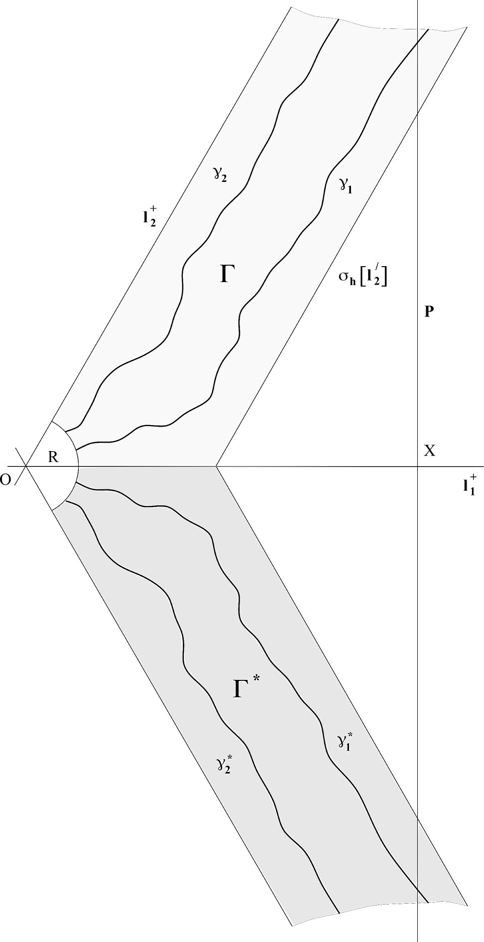
Consider a straight line orthogonal to and lying at a sufficient distance (to the right) from the intersection of the strips and (Fig. 9). Let be the intersection point of and .
The line forms a dense winding everywhere in
after factorization. We can therefore find an integer shift of a point () located at a distance of at most from the line and at a sufficiently large distance from .
The picture of level lines in the plane is identical to the picture in the plane . In particular, we can indicate here the stripes , , as well as the curves , , , , identical to those in the plane .
Let be the shortest vector connecting with the line (). It is easy to see that with a suitable choice of the point (in accordance with the above prescription) we can ensure the intersection of the curves and with the curves and in the plane (Fig. 10).
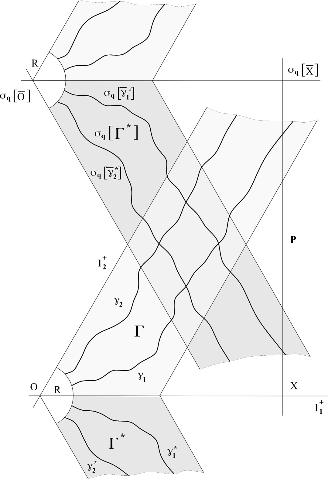
As a result, we arrive at the same contradiction as in situation A.
We have thus proved that under the conditions listed above, the emergence of open level lines for any potential of the above family is possible only at a single energy value . According to the general results of DynMalNovUMN , each specific potential from this family must have either open level lines or closed level lines of arbitrarily large sizes (or both) at the level .
All level lines of potentials at are closed. The sizes of closed level lines of all at are limited by one constant , which tends to infinity at . It should be said that the growth rate of in this limit depends significantly on the features of the initial potential (and, in particular, on the number of quasi-periods ).
III Conclusion
In this paper we consider the Novikov problem, i.e. the problem of describing the level lines of quasiperiodic functions on a plane, for quasiperiodic potentials admitting the dihedral symmetry . Potentials of this type can have only ‘‘chaotic’’ open level lines according to the general terminology dividing the open level lines of quasiperiodic functions into topologically regular and chaotic. Here we show that for an arbitrary number of quasiperiods, such potentials can have open level lines only at a single energy value . Such behavior of the open level lines, together with their complex geometry, brings these potentials close to random potentials on a plane, at the same time, such potentials also play an important role in the theory of two-dimensional quasicrystals. It can be noted that our results can also be useful for clarifying the connection between the geometry of open level lines and the features of their emergence in the energy interval in the general formulation of the Novikov problem.
References
- (1) S.P. Novikov, The Hamiltonian formalism and a many-valued analogue of Morse theory, Russian Math. Surveys 37 (5), 1-56 (1982).
- (2) A.V. Zorich, A problem of Novikov on the semiclassical motion of an electron in a uniform almost rational magnetic field., Russian Math. Surveys 39 (5), 287-288 (1984).
- (3) I.A. Dynnikov, Proof of S.P. Novikov’s conjecture for the case of small perturbations of rational magnetic fields, Russian Math. Surveys 47:3, 172-173 (1992).
- (4) S.P. Tsarev, private communication, 1992-1993
- (5) I.A. Dynnikov, Proof of S.P. Novikov’s conjecture on the semiclassical motion of an electron, Math. Notes 53:5, 495-501 (1993).
- (6) A.V. Zorich., Asymptotic Flag of an Orientable Measured Foliation on a Surface., Proc. ‘‘Geometric Study of Foliations’’., (Tokyo, November 1993), ed. T.Mizutani et al. Singapore: World Scientific Pb. Co., 479-498 (1994).
- (7) I.A. Dynnikov., Surfaces in 3-torus: geometry of plane sections., Proc. of ECM2, BuDA, 1996.
- (8) I.A. Dynnikov., Semiclassical motion of the electron. A proof of the Novikov conjecture in general position and counterexamples., Solitons, geometry, and topology: on the crossroad, Amer. Math. Soc. Transl. Ser. 2, 179, Amer. Math. Soc., Providence, RI, 1997, 45-73.
- (9) I.A. Dynnikov, The geometry of stability regions in Novikov’s problem on the semiclassical motion of an electron, Russian Math. Surveys 54:1, 21-59 (1999).
- (10) S.P. Novikov, A.Y. Maltsev, Topological quantum characteristics observed in the investigation of the conductivity in normal metals, JETP Letters 63 (10), 855-860 (1996).
- (11) S.P. Novikov, A.Y. Maltsev, Topological phenomena in normal metals, Physics-Uspekhi 41:3, 231-239 (1998).
- (12) A.Ya. Maltsev, S.P. Novikov., Quasiperiodic functions and Dynamical Systems in Quantum Solid State Physics., Bulletin of Braz. Math. Society, New Series 34:1 (2003), 171-210.
- (13) A.Ya. Maltsev, S.P. Novikov., Dynamical Systems, Topology and Conductivity in Normal Metals in strong magnetic fields., Journal of Statistical Physics 115:(1-2) (2004), 31-46.
- (14) A.Ya. Maltsev, S.P. Novikov, Topological integrability, classical and quantum chaos, and the theory of dynamical systems in the physics of condensed matter, Russian Math. Surveys, 74 (1), 141-173 (2019)
- (15) I.A. Dynnikov, A.Ya. Maltsev, S.P. Novikov, Geometry of quasi-periodic functions on the plane, Russian Math. Surveys 77 : 6, 1061–1085 (2022), arXiv:2306.11257
- (16) S.P. Novikov, Levels of quasiperiodic functions on a plane, and Hamiltonian systems, Russian Math. Surveys, 54 (5) (1999), 1031-1032
- (17) I.A. Dynnikov, S.P. Novikov, Topology of quasi-periodic functions on the plane, Russian Math. Surveys, 60 (1) (2005), 1-26
- (18) A.Ya. Maltsev, On the Novikov problem with a large number of quasiperiods and its generalizations, Proceedings of the Steklov Institute of Mathematics, 2024, Vol. 325, pp. 163–176, arXiv:2309.01475
- (19) A.Ya. Maltsev, S.P. Novikov, Open level lines of a superposition of periodic potentials on a plane, Annals of Physics 447(Pt.2), 169039 (2022)
- (20) A.V. Zorich., Finite Gauss measure on the space of interval exchange transformations. Lyapunov exponents., Annales de l’Institut Fourier 46:2, (1996), 325-370.
- (21) Anton Zorich., On hyperplane sections of periodic surfaces., Solitons, Geometry, and Topology: On the Crossroad, V. M. Buchstaber and S. P. Novikov (eds.), Translations of the AMS, Ser. 2, vol. 179, AMS, Providence, RI (1997), 173-189.
- (22) Anton Zorich., Deviation for interval exchange transformations., Ergodic Theory and Dynamical Systems 17, (1997), 1477-1499.
- (23) Anton Zorich., How do the leaves of closed 1-form wind around a surface., ‘‘Pseudoperiodic Topology’’, V.I.Arnold, M.Kontsevich, A.Zorich (eds.), Translations of the AMS, Ser. 2, vol. 197, AMS, Providence, RI, 1999, 135-178.
- (24) R. De Leo, Existence and measure of ergodic leaves in Novikov’s problem on the semiclassical motion of an electron., Russian Math. Surveys 55:1 (2000), 166-168.
- (25) R. De Leo, Characterization of the set of ‘‘ergodic directions’’ in Novikov’s problem of quasi-electron orbits in normal metals., Russian Math. Surveys 58:5 (2003), 1042-1043.
- (26) R. De Leo., Topology of plane sections of periodic polyhedra with an application to the Truncated Octahedron., Experimental Mathematics 15:1 (2006), 109-124.
- (27) Anton Zorich., Flat surfaces., in collect. ‘‘Frontiers in Number Theory, Physics and Geometry. Vol. 1: On random matrices, zeta functions and dynamical systems’’; Ecole de physique des Houches, France, March 9-21 2003, P. Cartier; B. Julia; P. Moussa; P. Vanhove (Editors), Springer-Verlag, Berlin, 2006, 439-586.
- (28) R. De Leo, I.A. Dynnikov, An example of a fractal set of plane directions having chaotic intersections with a fixed 3-periodic surface., Russian Math. Surveys 62:5 (2007), 990-992.
- (29) I.A. Dynnikov, Interval identification systems and plane sections of 3-periodic surfaces., Proceedings of the Steklov Institute of Mathematics 263:1 (2008), 65-77.
- (30) R. De Leo, I.A. Dynnikov., Geometry of plane sections of the infinite regular skew polyhedron ., Geom. Dedicata 138:1 (2009), 51-67.
- (31) A. Skripchenko., Symmetric interval identification systems of order three., Discrete Contin. Dyn. Sys. 32:2 (2012), 643-656.
- (32) A. Skripchenko., On connectedness of chaotic sections of some 3-periodic surfaces., Ann. Glob. Anal. Geom. 43 (2013), 253-271.
- (33) I. Dynnikov, A. Skripchenko., On typical leaves of a measured foliated 2-complex of thin type., Topology, Geometry, Integrable Systems, and Mathematical Physics: Novikov’s Seminar 2012-2014, Advances in the Mathematical Sciences., Amer. Math. Soc. Transl. Ser. 2, 234, eds. V.M. Buchstaber, B.A. Dubrovin, I.M. Krichever, Amer. Math. Soc., Providence, RI, 2014, 173-200, arXiv: 1309.4884
- (34) I. Dynnikov, A. Skripchenko., Symmetric band complexes of thin type and chaotic sections which are not actually chaotic., Trans. Moscow Math. Soc., Vol. 76, no. 2, 2015, 287-308.
- (35) A. Avila, P. Hubert, A. Skripchenko., Diffusion for chaotic plane sections of 3-periodic surfaces., Inventiones mathematicae, October 2016, Volume 206, Issue 1, pp 109–146.
- (36) A. Avila, P. Hubert, A. Skripchenko., On the Hausdorff dimension of the Rauzy gasket., Bulletin de la societe mathematique de France, 2016, 144 (3), pp. 539 - 568.
- (37) A.Ya. Maltsev, S.P. Novikov., The Theory of Closed 1-Forms, Levels of Quasiperiodic Functions and Transport Phenomena in Electron Systems., Proceedings of the Steklov Institute of Mathematics 302, 279-297 (2018).
- (38) Ivan Dynnikov, Pascal Hubert, Alexandra Skripchenko, Dynamical Systems Around the Rauzy Gasket and Their Ergodic Properties, International Mathematics Research Notices IMRN 2022, 1-30 (Published online), arXiv 2011.15043
- (39) A.Ya. Maltsev, On the Novikov problem for superposition of periodic potentials, arXiv:2409.09759
- (40) Le Thang Tu Quoc, S. A. Piunikhin, V. A. Sadov, The geometry of quasicrystals, Russian Mathematical Surveys 48 : 1 (1993), 37–100