The Quantum Optical Master Equation is of the same order of approximation as the Redfield Equation

Abstract

Quantum master equations are widely used to describe the dynamics of open quantum systems. All these different master equations rely on specific approximations that may or may not be justified. Starting from a microscopic model, applying the justified approximations only may not result in the desired Lindblad form preserving positivity. The recently proposed Universal Lindblad Equation is in Lindblad form and still retains the same order of approximation as the Redfield master equation [1]. In this work, we prove that the well-known Quantum Optical Master Equation is also in the same equivalence class of approximations. We furthermore compare the Quantum Optical Master Equation and the Universal Lindblad Equation numerically and show numerical evidence that the Quantum Optical Master Equation yields more accurate results.

I Introduction

The characterization and description of open quantum systems is an important problem that has been studied for a long time [2]. It is relevant for many fields, including atomic, molecular, and optical physics. Its significance extends especially to the field of quantum information processing [3], where describing open quantum systems helps to understand and develop control techniques [4].

A powerful tool in the study of these open quantum systems are quantum master equations. Their validity, however, is often unclear, as it typically relies on uncontrolled approximations [2]: starting from the exact Liouville-Von Neumann equation, one performs the standard Born (assuming weak coupling between system of interest and its environment) and Markov approximations (assuming short bath memory) to derive the Redfield equation [5].

A more general approach to derive a master equation to describe an open quantum system is the Nakajima-Zwanzig formalism [6, 7]. In its most general form, it leads to a formally exact master equation. This equation is then usually truncated to get an approximate but more easily solvable master equation, although the validity of these approximations is not always clear [8]. The aforementioned Redfield equation emerges as the lowest order approximation of the Nakajima-Zwanzig equation [2].

However, the Redfield equation is not a Lindblad master equation, which in particular means that it does not preserve positivity [9, 10, 11]. The traditional way to achieve Lindblad form is another approximation called the secular approximation. This approximation is usually performed heuristically by neglecting ”fast oscillating terms”. The resulting equation is known as the Quantum Optical Master Equation (QOME) and offers a range of advantages compared to the Redfield Equation [2]. First, being in Lindblad form, it preserves positivity and so guarantees physicality of the result. Furthermore, a master equation in Lindblad form can alternatively be solved numerically by stochastic evolution of pure states [2, 12].

In this work we show that the QOME is of the same order of approximation as the Redfield equation. For this purpose we present a novel, systematic derivation of the QOME, resulting in the exact same result as applying the secular approximation. By doing this we see that to derive the QOME from the Redfield Equation we do not need to drop terms of higher order as those already neglected for deriving the Redfield equation. This is done by a general, systematic approach, only using tools for solving systems of ordinary differential equations.

The Universal Lindblad Equation (ULE) has been shown to be of the same order of approximation as the Redfield equation too [1]. The result of this work shows that the Quantum Optical master equation belongs to the same equivalence class of Markov approximations as the Redfield equation and the Universal Lindblad equation. We furthermore give analytical considerations as well as numerical evidence indicating that the QOME outperforms the ULE.

We present the rigorous derivation of the QOME in section II. We start by giving a brief overview of the Nakajima-Zwanzig approach to derive the Nakajima-Zwanzig Master Equation in section II.1. We show how this equation is approximated to the Redfield equation and give an explicit form for the Redfield tensor. This enables us to formally derive the QOME from the Redfield equation in section II.2 while showing that none of the further neglected terms are of higher order than those already neglected to get to the Redfield equation. This proves that the thus obtained QOME is of the same order of approximation as the Redfield Equation. We furthermore provide an analytical consideration which suggests that the QOME yields more accurate results than the Universal Lindblad Equation in section II.3.

In section III, we show that, for certain examples, the numerical solution of the QOME indeed shows a higher similarity to that of the Redfield equation than that of the ULE. Hence, while the ULE does not rely on knowledge of the system eigenstates, the numerics indicate that the QOME is a more accurate alternative for systems where the energy structure is known.

II The Lindblad Master Equation

II.1 Derivation of the Redfield Equation

In the theory of open quantum systems, the state of a system at time $t$ is described by a Hermitian, positive semi-definite matrix $\hat{\rho}(t)$ with ${\rm Tr}[\hat{\rho}(t)]=1$ called the density matrix [2]. To describe its dynamics, it is therefore desirable to use a quantum master equation that preserves these properties for any $t$, that is, it has to be completely positive and trace-preserving. As proven by Lindblad in 1976, such a master equation can always be written in the form

$$\frac{{\rm d}}{{\rm d}t}\hat{\rho}(t)= -i\left[\hat{H},\hat{\rho}(t)\right]$$ (1)

$$+\sum_{k}\gamma_{k}\left(\hat{L}_{k}\hat{\rho}(t)\hat{L}_{k}^{\dagger}-\frac{1}{2}\left\{\hat{L}_{k}^{\dagger}\hat{L}_{k},\hat{\rho}(t)\right\}\right).$$

Here, the time evolution of the density matrix $\hat{\rho}(t)$ is fully determined by a unitary part, generated by the Hamiltonian $\hat{H}$, and a dissipative part given by the Lindblad operators $\hat{L}_{k}$. Eq. (1) has been applied to many tasks within a wide range of research fields, from quantum optics [13, 14] and atomic physics [15, 16, 17] to quantum information [18, 19, 20, 21, 22] and many more.
Although the form of the desired master equation is known, it remained an open question how to derive such a master equation accurately based on a microscopic model in general. For example, Ref. [14] illustrates well how the use of a wrong Lindblad equation can lead to discrepancies between experiments and the theory describing them. Hence, given a quantum system of interest described by the Hamiltonian $\hat{H}_{\rm S}$ that couples to an environment described by the Hamiltonian $\hat{H}_{\rm B}$, how do the correct Lindblad operators $\hat{L}_{k}$ in Eq. (1) look like to capture the system dynamics accurately?

We consider a total quantum system described by the Hamiltonian

$$\hat{H}=\hat{H}_{\rm S}+\hat{H}_{\rm B}+g\hat{H}_{\rm int}.$$ (2)

Here, $\hat{H}_{S}$ and $\hat{H}_{B}$ denote the Hamiltonians corresponding to the quantum system of interest S resp. the bath B, and the interaction between system and bath and with dimensionless coupling strength $g\ll 1$ is described by the Hamiltonian

$$\hat{H}_{\rm int}=\sum_{\alpha}\hat{S}_{\alpha}\otimes\hat{B}_{\alpha}$$ (3)

that can be decomposed in operators $\hat{S}_{j}$ and $\hat{B}_{j}$ acting respectively on the system and on the bath only.

The standard way to derive a quantum master equation in Lindblad form is to derive the Redfield master equation first, and to apply the secular approximation afterwards [5, 2]. In the following, we show that we can achieve the same result by only dropping terms which are of same order than those we already dropped to derive the Redfield equation.

There are plenty of ways to derive the Redfield master equation, like the phenomenological approach by Redfield himself by applying the standard Born and Markov approximations [5], or the Bogoliubov method [11, 23]. Here, we use the systematic derivation of the Redfield master equation using projection operator techniques as presented in Ref. [2], chapter 9.

Using this, we arrive at a master equation in the interaction picture which reads

$$\frac{{\rm d}}{{\rm d}t}\hat{\tilde{\rho}}_{\rm S}(t) \,=-g^{2}\int_{0}^{t}{\rm d}s$$ (4)

$$\left({\rm Tr}_{\rm B}\left[\hat{H}_{\rm int}(t)\right.,\left.\left[\hat{H}_{\rm int}(t-s),\hat{\tilde{\rho}}_{\rm S}(t)\otimes\hat{\tilde{\rho}}_{\rm B}\right]\right]\right)$$

$$+\,\mathcal{O}\left(g^{4}\right),$$

where we have denoted the density operator of the system and bath by $\hat{\rho}_{S}$ and $\hat{\rho}_{B}$ respectively, and their interaction picture counterparts as $\hat{\tilde{\rho}}_{S}$ and $\hat{\tilde{\rho}}_{B}$.

By dropping the terms of $\mathcal{O}(g^{4})$, Eq. (4) becomes the well-known Redfield equation. This equation can not be written in Lindblad form. In particular, Eq. (4) does not guarantee to preserve positivity [24].

Let now $\varepsilon_{k}$ be the eigenfrequencies of $\hat{H}_{\rm S}$ such that $\hat{\Pi}(k)$ projects onto the subspace indexed by $k$. We can write Eq. (4) in the Schrödinger picture using the definitions

$$\hat{S}_{\alpha}(\omega)=\sum_{\varepsilon_{k}-\varepsilon_{k^{\prime}}=\omega}\hat{\Pi}(k)\hat{S}_{\alpha}\hat{\Pi}(k^{\prime})$$ (5)

and

$$\Gamma_{\alpha\beta}(\omega)=g^{2}\int_{0}^{t}e^{i\omega s}\mathcal{B}_{\alpha\beta}(s){\rm d}s$$ (6)

with the bath correlation functions

$$\mathcal{B}_{\alpha\beta}(s)= {\rm Tr}_{\rm B}\left[\hat{B}_{\alpha}(t)\hat{B}_{\beta}(t-s)\hat{\rho}_{\rm B}\right]$$

$$= \left\langle\hat{B}_{\alpha}(s)\hat{B}_{\beta}(0)\right\rangle,$$ (7)

resulting in

$$\frac{{\rm d}}{{\rm d}t}\hat{\rho}_{\rm S}(t)=-i\left[\hat{H}_{\rm S},\hat{\rho}_{\rm S}(t)\right]+\hat{R}\hat{\rho}_{\rm S}(t),$$ (8)

with the Redfield tensor

$$\hat{R}\hat{\rho}(t) =\displaystyle{\sum_{\omega,\nu}\sum_{\alpha,\beta}}\Gamma_{\alpha\beta}(\omega)\left(\hat{S}_{\beta}(\omega)\hat{\rho}(t)\hat{S}^{\dagger}_{\alpha}(\nu)-\hat{S}^{\dagger}_{\alpha}(\nu)\hat{S}_{\beta}(\omega)\hat{\rho}(t)\right)+\text{H.c.},$$

where we dropped the subscript S to shorten the notation, since from now on the considered density matrix is always the one of that system of interest S. In an eigenbasis of the system Hamiltonian, Eq. (8) written in component form becomes

$$\frac{{\rm d}}{{\rm d}t}\rho_{ab}(t)=-i\omega_{ab}\rho_{ab}(t)+\sum_{j,k}R_{abjk}\rho_{ab}(t),$$ (9)

where $\omega_{jk}=\varepsilon_{j}-\varepsilon_{k}$ denote the energy differences. Note that the matrix elements of $\hat{R}$ satisfy $R_{abjk}=\mathcal{O}\left(g^{2}\right)$ and

$$\left(\hat{R}\rho(t)\right)_{ab}=\bra{a}\hat{R}\rho(t)\ket{b}=\sum_{j,k}R_{abjk}\rho_{jk}.$$ (10)

We first explicitly calculate the term

$$\bra{a}\hat{S}_{\beta}(\omega)\hat{\rho}(t)\hat{S}_{\alpha}^{\dagger}(\nu)\ket{b}$$

$$=\sum_{\stackrel{{\scriptstyle n,m,}}{{\omega_{nm}=\omega}}}\sum_{\stackrel{{\scriptstyle p,l,}}{{\omega_{pl}=\nu}}}\bra{a}\ket{n}\bra{n}\hat{S}_{\beta}\ket{m}\bra{m}\rho(t)\ket{l}\bra{l}\hat{S}_{\alpha}\ket{p}\bra{p}\ket{b}$$

$$=\sum_{\stackrel{{\scriptstyle m,}}{{\omega_{am}=\omega}}}\sum_{\stackrel{{\scriptstyle l,}}{{\omega_{bl}=\nu}}}\bra{a}\hat{S}_{\beta}\ket{m}\bra{l}\hat{S}_{\alpha}\ket{b}\rho_{ml}(t).$$ (11)

We can do the same for the other terms in Eq. (II.1) and then compare the coefficients in the sum in Eq. (10). We observe that the elements of the Redfield tensor can be rewritten as

$$R_{abjk} =$$

$$\sum_{\omega,\nu}\left(\mathcal{S}^{\left({1}\right)}_{ab,\omega\nu,jk}-\mathcal{S}^{\left({2}\right)}_{ab,\omega\nu,jk}+\mathcal{S}^{\left({3}\right)}_{ab,\omega\nu,jk}-\mathcal{S}^{\left({4}\right)}_{ab,\omega\nu,jk}\right),$$

using the definition

$$\mathcal{S}^{\left({1}\right)}_{ab,\omega\nu,jk} =\sum_{\alpha,\beta}\Gamma_{\alpha\beta}(\omega)$$ (13)

$$\sum_{\stackrel{{\scriptstyle m}}{{\omega_{am}=\omega}}}\sum_{\stackrel{{\scriptstyle l}}{{\omega_{bl}=\nu}}}\langle a|\hat{S}_{\beta}|m\rangle\langle l|\hat{S}_{\alpha}|b\rangle\delta_{mj}\delta_{lk}$$

and similar definitions for $\mathcal{S}^{\left({p}\right)}_{ab,\omega\nu,jk},p\in\{1,2,3,4\}$.

In the next section, we show that there is a systematic method to perform the secular approximation. We will use this method to simplify Eq. (II.1). This will yield an equation that is equivalent to the Redfield equation in approximation order, but is a Lindblad master equation.

II.2 The Secular Approximation

Note that to get to the Redfield equation, we neglect all terms of order $\mathcal{O}\left(g^{4}\right)=\mathcal{O}\left(R^{2}\right)$ in Eq. (4). Any approximation which only leaves out terms of this order will therefore be equivalent in approximation order. As we show in the following, this enables us to show that the QOME indeed is of the same approximation order than the Redfield Equation.

We start by vectorizing Eq. (9), which reduces the problem of solving the differential equation to solving the characteristic equation of a matrix. We show that we can neglect certain terms in this characteristic equation. This leads to the double sums in Eq. (II.1) reducing to a single sum over one parameter, which corresponds to the usual way of applying the secular approximation.

First, we vectorize Eq. (9). For the indices $i,j,$ $k,l$ $\in\{n\in\mathbb{N},n<z\}$ in matrix form we define

$$c=iz+j,d=kz+l\in\{n\in\mathbb{N},n<z^{2}-1\},$$ (14)

so for example in the one qubit case the vectorized density matrix can be written as

$$\hat{\rho}(t)=\left(\begin{array}[]{rr}\rho_{00}(t)&\rho_{01}(t)\\ \rho_{10}(t)&\rho_{11}(t)\end{array}\right)\longrightarrow\underline{\rho}(t)=\left(\begin{array}[]{c}\rho_{00}(t)\\ \rho_{01}(t)\\ \rho_{10}(t)\\ \rho_{11}(t)\end{array}\right).$$ (15)

For the density matrix and the frequencies in the Redfield Eq. (9)) we get

$$\rho_{c}=\rho_{ij}\textnormal{ and }\omega_{c}=\omega_{ij}.$$ (16)

We then define the matrices $\mathcal{H}$ with

$$\mathcal{H}_{cd}=-i\cdot\textnormal{diag}\left(\omega_{0},\omega_{1},\dots,\omega_{z^{2}-1}\right)$$ (17)

and $\mathcal{R}$ with

$$\mathcal{R}_{cd}=R_{ijkl}.$$ (18)

The Redfield Eq. (9) can be written as

$$\frac{{\rm d}}{{\rm d}t}\underline{\rho}(t)=\left(\mathcal{H}+\mathcal{R}\right)\underline{\rho}(t).$$ (19)

This system of ordinary differential equations can be solved by the eigenanalysis method. The general solution is given by [25]

$$\underline{\rho}(t)=\sum_{j}c_{j}e^{s_{j}t}\underline{v}_{j},$$ (20)

where $s_{j}$ and $\underline{v}_{j}$ are the eigenvalues and eigenvectors of $\mathcal{H}+\mathcal{R}=:\mathcal{M}$. Plugging in $\underline{\rho}(0)=\underline{\rho}_{0}$ gives the unique solution to the initial value problem.

The characteristic equation is given by $\det\left(\mathcal{A}(s)\right)=0$ of $\mathcal{M}$, where $\mathcal{A}(s)=-s\mathbb{I}+\mathcal{H}+\mathcal{R}$. Note again that in the derivation of Eq. (9), we neglected terms of order $\mathcal{O}(g^{4})$. This means if we drop these in the characteristic equation, the solution will be of the same order of approximation. In the following, our goal is to show that if we do that, we in fact get back the QOME.

For the following considerations, we distinguish between two types of eigenvalues. Since $\mathcal{H}$ is diagonal, the eigenvalues $s_{j}$ of $\mathcal{M}$ have to be of the form $s_{j}=i\omega_{j}+\delta s_{j}$, with $\delta s_{j}=\mathcal{O}(\mathcal{R})$. Note that $\mathcal{O}(\mathcal{R})=\mathcal{O}(g^{2})$ as the Redfield tensor is of order $\mathcal{O}(g^{2})$. If $\omega_{j}=0$, then we call $s_{j}$ an incoherent pole. If $\omega_{j}\neq 0$, then we call $s_{j}$ a coherent pole.

We first consider all the diagonal elements of $\mathcal{A}$ that are of order $\mathcal{O}(\mathcal{R})$. We define the set

$$D=\left\{\left.d\in\left\{0,\dots,z^{2}-1\right\}\right|\mathcal{A}_{dd}\in\mathcal{O}(\mathcal{R})\right\}.$$ (21)

This is a finite set. We call its number of elements $n_{D}:=\#D$ and index its elements by $d_{0},\ldots d_{n_{D}-1}$. Note that if $c\notin D$, then $\mathcal{A}_{cc}=\mathcal{O}(g^{0})$. Furthermore, we have $\mathcal{A}_{cd}\in\mathcal{O}(g^{2})$ for $c\neq d$, since $\mathcal{H}$ is diagonal. Now, we compute the determinant using Leibniz formula. It follows

$$\det\left({\mathcal{A}\left({s}\right)}\right) =\displaystyle{\sum_{\tau\in S_{z^{2}}}{\rm sgn}\left({\tau}\right)\prod_{i=0}^{z^{2}-1}\mathcal{A}_{i,\tau\left({i}\right)}\left({s}\right)}$$ (22)

$$=\displaystyle{\underbrace{\left(\prod_{\stackrel{{\scriptstyle i=0}}{{i\notin D}}}^{z^{2}-1}\mathcal{A}_{ii}\left({s}\right)\right)}_{\mathcal{O}(g^{0})}\underbrace{\sum_{\tau\in U_{D}}{\rm sgn}\left({\tau}\right)\prod_{k\in D}\mathcal{A}_{k,\tau\left({k}\right)}\left({s}\right)}_{{\mathcal{O}\left({g^{2n_{D}}}\right)}}}$$

$$+\mathcal{O}\left({g^{2(n_{D}+1)}}\right),$$

where $U_{D}=\left\{{\tau\in S_{z^{2}},\tau\left({i}\right)=i\;\forall\;i\notin D}\right\}$. By definition, $\mathcal{A}_{ii}$ is of order $\mathcal{O}(1)$ for $i\notin D$. For all other $c,d$ we have by definition $\mathcal{A}_{cd}\in\mathcal{O}\left({g^{2}}\right)$. The first term on the right hand side of Eq. (22) is therefore of order $\mathcal{O}\left({g^{2n_{D}}}\right)$. Furthermore, since $A_{ii}$ for $i\notin D$ are the only elements of $\mathcal{A}$ which are not or order $\mathcal{O}\left({g^{2}}\right)$. This means that, except for the aforementioned first term, all other terms contained in the determinant are at least of order $\mathcal{O}\left({g^{2(n_{D}+1)}}\right)$.

Let us consider the equation

$$\det\left(\mathcal{A}(s)\right)=0.$$ (23)

We now apply a self-consistency argument. To derive the Redfield equation from the Nakajima-Zwanzig equation (Eq. (4)), we only kept the terms in the equation that are of lowest order in $g$, so terms of order $\mathcal{O}(g^{2})$. All terms of higher order, namely those of order $\mathcal{O}(g^{4})$ were dropped. For the determinant, as illustrated above, the terms of lowest order in $g$ are of order $\mathcal{O}(g^{2n_{D}})$ Therefore, to apply this approximation consistently here, we drop all terms that are of order $\mathcal{O}\left({g^{2(n_{D}+1)}}\right)$. This leaves us with the equation

$$\left(\prod_{\stackrel{{\scriptstyle i=0}}{{i\notin D}}}^{z^{2}-1}\mathcal{A}_{ii}\left({s}\right)\right)\sum_{\tau\in U_{D}}{\rm sgn}\left({\tau}\right)\prod_{k\in D}\mathcal{A}_{k,\tau\left({k}\right)}\left({s}\right)=0,$$ (24)

where we can factor out $\left(\prod_{\stackrel{{\scriptstyle i=0}}{{i\notin D}}}^{z^{2}-1}\mathcal{A}_{ii}\left({s}\right)\right)\neq 0$ to obtain

$$\sum_{\tau\in U_{D}}{\rm sgn}\left({\tau}\right)\prod_{k\in D}\mathcal{A}_{k,\tau\left({k}\right)}\left({s}\right)=:\det\left({\tilde{\mathcal{A}}\left({s}\right)}\right)=0.$$ (25)

Here, we defined the $n_{D}\times n_{D}$-matrix $\tilde{\mathcal{A}}$ as

$$\tilde{\mathcal{A}}=\left({\tilde{\mathcal{A}}_{ij}\left({s}\right)}\right)_{i,j\in\left\{{0,\dots,n_{D}-1}\right\}}\textnormal{ with }\tilde{\mathcal{A}}_{ij}\left({s}\right)=\mathcal{A}_{d_{i}d_{j}}\left({s}\right).$$ (26)

We can visualize this process by the matrix represented in fig. 1. All the nondiagonal terms of this matrix are of order $\mathcal{O}(g^{2})$. Only on the diagonal, we can have terms of order $\mathcal{O}(g^{0})$. This means that the term of lowest order in $g$ has to be the product of all diagonal elements. Furthermore, any permutation that leads to a term of the same order has to only swap out diagonal elements of order $\mathcal{O}(g^{2})$. All of these permutations are contained in the set $U_{D}$.

This means we can restrict ourselves to only calculating the determinant of the reduced matrix $\tilde{\mathcal{A}}$. This is equivalent to the fact that, instead of $\mathcal{R}$, we only consider the reduced matrix

$$\tilde{\mathcal{R}}=\left({\tilde{\mathcal{R}}_{ij}\left({s}\right)}\right)_{i,j\in\left\{{0,\dots,n_{D}-1}\right\}}\textnormal{ with }\tilde{\mathcal{R}}_{ij}\left({s}\right)=\mathcal{R}_{d_{i}d_{j}}\left({s}\right).$$ (27)

The elements contained in the reduced matrix $\tilde{R}$ depend on the set $D$, which differs for coherent and incoherent poles. For coherent poles, we have

$$\mathcal{A}_{dd}=-i\omega_{c}+\delta_{s}+i\omega_{d}+R_{dd}\in\mathcal{O}(\mathcal{R})\Leftrightarrow\omega_{d}=\omega_{c},$$ (28)

or equivalently

$$D=\left\{{d\in\left\{{0,\dots,z^{2}-1}\right\};\;\omega_{d}\neq 0;\;\omega_{d}=\omega_{c}}\right\}.$$ (29)

For incoherent poles, we have $s=\delta_{s}\in\mathcal{O}(\mathcal{R})$, such that

$$\mathcal{A}_{dd}=\delta_{s}+i\omega_{d}+R_{dd}\in\mathcal{O}(\mathcal{R})\Leftrightarrow\omega_{d}=0,$$ (30)

hence

$$D=\left\{{d\in\left\{{0,\dots,z^{2}-1}\right\};\;\omega_{d}=0}\right\}.$$ (31)

$$\begin{pmatrix}\mathcal{O}(\mathcal{R})&\cdots&\square&\cdots&\square&\cdots&\square&\cdots\\ \vdots&\ddots&\vdots&&\vdots&&\vdots\\ \square&\cdots&\mathcal{O}(\mathcal{R})&\cdots&\square&\cdots&\square&\cdots\\ \vdots&&\vdots&\ddots&\vdots&&\vdots\\ \square&\cdots&\square&\cdots&\mathcal{O}(\mathcal{R})&\cdots&\square&\cdots\\ \vdots&&\vdots&&\vdots&\ddots&\vdots\\ \square&\cdots&\square&\cdots&\square&\cdots&\mathcal{O}(\mathcal{R})&\cdots\\ \vdots&&\vdots&&\vdots&&\vdots&\ddots\end{pmatrix}$$ (32)

Figure 1: Illustration of the simplification process for the matrix. Only permutations that swap $\mathcal{O}(\mathcal{R})$-elements on the diagonal are of lowest order in $\mathcal{R}$. This means we only have to consider the determinant of the reduced matrix $\tilde{\mathcal{A}}$, which consists of the $\mathcal{O}(\mathcal{R})$-elements together with the squares in the figure.

In both cases, the remaining matrix elements $\tilde{\mathcal{R}}_{ij}$ satisfy $\omega_{i}=\omega_{j}$. Going back to the non-vectorised notation $R_{abjk}$, we find

$$\omega_{ab}=\varepsilon_{a}-\varepsilon_{b}=\omega_{c}=\varepsilon_{j}-\varepsilon_{k}=\omega_{jk}.$$ (33)

We found a condition for $R_{abjk}$ to be negligible, namely that $\omega_{ab}=\omega_{jk}$. This condition we insert in the definition (13) of $\mathcal{S}^{\left({1}\right)}_{ab,\omega\nu,jk}$. We note that by definition for any contribution to $\mathcal{S}^{\left({1}\right)}_{ab,\omega\nu,jk}$, we have

$$\omega_{aj}=\varepsilon_{a}-\varepsilon_{j}=\omega\textnormal{ and }\omega_{bk}=\varepsilon_{b}-\varepsilon_{k}=\nu,$$ (34)

which implies using Eq. (33) that

$$\nu=\varepsilon_{b}-\varepsilon_{k}=\left({\varepsilon_{a}-\omega_{c}}\right)-\left({\varepsilon_{j}-\omega_{c}}\right)=\varepsilon_{a}-\varepsilon_{j}=\omega.$$ (35)

We obtain the same result for the other $\mathcal{S}^{\left({p}\right)}_{ab,\omega\nu,jk}$ analogously. To conclude, by neglecting terms of higher than the lowest order in $\mathcal{R}$, we rediscover exactly the standard secular approximation. Eq. (II.1) becomes

$$\hat{R}\hat{\rho}(t) =\displaystyle{\sum_{\omega}\sum_{\alpha,\beta}}\Gamma_{\alpha\beta}(\omega)\left(\hat{S}_{\beta}(\omega)\hat{\rho}(t)\hat{S}^{\dagger}_{\alpha}(\omega)-\hat{S}^{\dagger}_{\alpha}(\omega)\hat{S}_{\beta}(\omega)\hat{\rho}(t)\right)+\text{H.c.}$$ (36)

It is known that this equation can be cast into Lindblad form [2] by splitting up the coefficients

$$\Gamma_{\alpha\beta}(\omega)=\frac{1}{2}\gamma_{\alpha\beta}(\omega)+i\imaginary(\Gamma_{\alpha\beta}(\omega))$$ (37)

with

$$\gamma_{\alpha\beta}(\omega)=2\real\left(\Gamma_{\alpha\beta}(\omega)\right)=g^{2}\int_{-t}^{t}e^{i\omega s}\mathcal{B}_{\alpha\beta}(s){\rm d}s.$$ (38)

Diagonalizing the coefficient matrix $\left(\Gamma_{\alpha\beta}(\omega)\right)_{\alpha,\beta}$ yields

$$\hat{R}\hat{\rho}(t)=-i\left[\hat{H}_{\rm LS},\hat{\rho}(t)\right]$$

$$+\sum_{\omega,q}\gamma_{q}(\omega)\left(\hat{S}_{q}(\omega)\hat{\rho}(t)\hat{S}_{q}(\omega)^{\dagger}-\frac{1}{2}\left\{\hat{S}_{q}(\omega)^{\dagger}\hat{S}_{q}(\omega),\hat{\rho}(t)\right\}\right)$$

with the Lamb shift Hamiltonian

$$\hat{H}_{\rm LS}=\sum_{\omega,q}\imaginary\left(\Gamma_{q}(\omega)\right)\hat{S}_{q}(\omega)^{\dagger}\hat{S}_{q}({\omega}).$$ (40)

We finally arrive at the quantum master equation in Lindblad form

$$\frac{{\rm d}}{{\rm d}t}\hat{\rho}(t)=\mathcal{L}_{\text{QOME}}\hat{\rho}=-i\left[\hat{H}_{\rm S}+\hat{H}_{\rm LS},\hat{\rho}(t)\right]$$

$$+\sum_{\omega,q}\gamma_{q}(\omega)\left(\hat{S}_{q}(\omega)\hat{\rho}(t)\hat{S}_{q}(\omega)^{\dagger}-\frac{1}{2}\left\{\hat{S}_{q}(\omega)^{\dagger}\hat{S}_{q}(\omega),\hat{\rho}(t)\right\}\right).$$

(41)

This is the well-known Quantum Optical Master Equation (QOME) [2]. We conclude that this equation is of the same order of approximation as the Redfield equation.

The presented derivation shall be understood as the formalization of the secular approximation. We systematically remove terms of higher order in the coupling strength $g$ between system and bath. As a result, we obtain the Quantum Optical Master Equation naturally, as we would by applying the secular approximation in the traditional, heuristic way.

II.3 Comparison to Universal Lindblad

Eq. (41) is in Lindblad form, but of the same order of approximation in the bath coupling strength $g$ as the Redfield equation. The fact that there is an equation in Lindblad form that is of the same approximation order as the Redfield equation is nothing new though. In fact, Rudner and Nathan have shown that there is another such equation, the ULE [1]. The difference to the result obtained here is that the ULE boasts only one Lindblad operator $L_{\text{UL}}$ for each $q$.

It relates to Eq. (41) in that the sum over $\omega$ of the Lindblad operators in that equation equate the Universal Lindblad operator, so

$$L_{q}^{(\text{UL})}=\sum_{\omega}\sqrt{\gamma_{q}(\omega)}\hat{S}_{q}(\omega).$$ (42)

We give an analytical intuition for the better accuracy of the Quantum Optical Master Equation compared to the Universal Lindblad Equation. Following Ref. [1], the Redfield equation in the interaction picture takes the form

$$\dot{\tilde{\rho}}(t)=\int_{-\infty}^{\infty}\differential t^{\prime}\int_{-\infty}^{\infty}\differential s\mathcal{F}(t,s,t^{\prime})[\tilde{\rho}]$$ (43)

with

$$\mathcal{F}(t,s,t^{\prime})[A] =\gamma\theta(t-t^{\prime})g(t-s)g(s-t^{\prime})[\tilde{S}(t),A(\tilde{S}(t^{\prime})]$$

$$+\text{H.c.}$$ (44)

and

$$g(s)=\frac{1}{\sqrt{2\pi}}\int_{-\infty}^{\infty}\differential\nu\sqrt{J(\nu)}e^{-i\omega s}$$ (45)

with the bath spectral function $J$.

Now we transform back to the Schrödinger picture. We get

$$\dot{\tilde{\rho}}(t)=i[H_{S},\tilde{\rho}(t)]+R\tilde{\rho}(t)$$ (46)

with

$$R\tilde{\rho}(t) =\int_{-\infty}^{\infty}\differential t^{\prime}\int_{-\infty}^{\infty}\differential sU^{\dagger}(t)\mathcal{F}(t,s,t^{\prime})U(t)$$

$$=\int_{-\infty}^{\infty}\differential t^{\prime}\int_{-\infty}^{\infty}\differential s\left(S\tilde{\rho}(t)e^{iH_{S}(t-t^{\prime})}Se^{-iH_{S}(t-t^{\prime})}\right.$$

$$-\left.\tilde{\rho}(t)e^{iH_{S}(t-t^{\prime})}Se^{-iH_{S}(t-t^{\prime})}S\right)+\text{H.c.}$$ (47)

We now restrict ourselves to the single qubit case. We assume a system Hamiltonian $H_{S}=\epsilon\sigma_{z}+\Delta\sigma_{x}$. In its eigenbasis, the previous equation reads

$$R\tilde{\rho}(t) =\int_{-\infty}^{\infty}\differential t^{\prime}\int_{-\infty}^{\infty}\differential s\left[\gamma\theta(t-t^{\prime})g(t-s)g(s-t^{\prime})\right.$$

$$\phantom{+}\left.\sum_{a,b,c,d}e^{i\omega_{dc}(t-t^{\prime})}\bra{a}S\ket{b}\bra{c}S\ket{d}\ket{a}\bra{b}\rho(t)\ket{c}\bra{d}\right.$$

$$+\left.\sum_{a,b,c,d}e^{i\omega_{ab}(t-t^{\prime})}\bra{a}S\ket{b}\bra{c}S\ket{d}\delta_{cb}\rho(t)\ket{a}\bra{d}\right]$$

$$+\text{H.c.},$$ (48)

where $\ket{a}$ are the eigenstates of $H_{S}$. We calculate the terms for the Redfield tensor by

$$R_{abcd}=\bra{a}(R\ket{c}\bra{d})\ket{b}.$$ (49)

We now consider for simplicity a system with $S=\sigma_{z}$ and $H_{S}=\sigma_{x}$ and $E_{0}=1$ and $E_{1}=-1$ being the eigenenergies of $H_{S}$. Defining $\omega=E_{0}-E_{1}$ enables us to write down the Redfield superoperator with $\mathcal{R}_{an+b,cn+d}=R_{abcd}$ explicitly as

$$\mathcal{R}=\begin{pmatrix}G(\omega)+G(-\omega)&0&0&G(\omega)+G(-\omega)\\ 0&2G(-\omega)&2G(\omega)&0\\ 0&2G(-\omega)&2G(\omega)&0\\ G(\omega)+G(-\omega)&0&0&G(\omega)+G(-\omega)\end{pmatrix}$$ (50)

with

$$G(\omega) =\int_{-\infty}^{\infty}\differential t^{\prime}\int_{-\infty}^{\infty}\differential s$$

$$\gamma\theta(t-t^{\prime})g(t-s)g(s-t^{\prime})e^{i\omega(t-t^{\prime})}.$$ (51)

We describe the two approaches to bring the Redfield equation into Lindblad form:

• For the Quantum Optical Master Equation, we remove all the terms except $\mathcal{R}_{00},\mathcal{R}_{03},\mathcal{R}_{30},\mathcal{R}_{33}$.

• For the Universal Lindblad equation, we replace the function $G$ by the function $F$ defined by [1]

  $$F(\omega) =\int_{-\infty}^{\infty}\differential s^{\prime}\int_{-\infty}^{\infty}\differential s$$

  $$\gamma\theta(s-s^{\prime})g(s-t)g(t-s)e^{i\omega(t-s^{\prime})}.$$ (52)

Figure 2: Change to the Redfield equation by the Universal Lindblad (UL) and the Quantum Optical (QO) master equations. We see that in the case of the Universal Lindblad equation, in addition to the matrix elements that can be compared to $\omega$, the other matrix elements are also changed.

The changes made by the Quantum Optical Master Equation and the Universal Lindblad Equation are visualized in Eq. (2)). We see that for this simple case, the terms removed by application of the secular aproximation are only the ones which are dominated by $\omega$ anyways. In the Universal Lindblad case, the other matrix elements are changed as well. Since in the weak coupling limit, $\omega$ is large compared to $G(\omega)$ or $F(\omega)$, changing $F$ to $G$ in terms containing $\omega$ has little effect on the solution. However, in the case of the Universal Lindblad Equation, even terms that are not dominated by $\omega$ are changed, which leads to a higher divergence from the solution of the Redfield equation than in the case of the Quantum Optical Master Equation.

In the following section, we do a numerical comparison of the two equations by applying both to a toy model and comparing both solutions to the solution of the Redfield equation. We see that the numerical results for the toy model confirm the above expectations.

III Numerical Demonstrations

So far, we performed the secular approximation to the Redfield Eq. (8) in a novel way to achieve the QOME in Lindblad form of Eq. (41). This derivation reproduced the well-known result that we would get if we just threw away the “fast oscillating terms” instead.

In this section, we are going to apply the QOME to benchmark its performances against the ULE for a Two-Level-System (TLS) The single-particle Hamiltonian describing the TLS is given by

$$\hat{H}_{S}=E\Bigl{(}\cos(\phi)\hat{\sigma}_{z}+\sin(\phi)\hat{\sigma}_{x}\Bigr{)},$$ (53)

where $E$, $\phi$ are some constants describing the qubit energy and orientation in the Bloch sphere, respectively; also we have to consider the interaction with the environment, that we are going to model as an Ohmic or Jaynes-Cummings-like bath.

Ohmic baths are ubiquitous in high frequency ($\gtrsim$1\text{\,}\mathrm{GHz}$$) spectroscopy accounting for Nyquist noise [26], the Ohmic spectral density function bath reads

$$J(\omega)=\alpha\omega\frac{{\Omega}^{2}}{\Omega^{2}+\omega^{2}},$$ (54)

where $\alpha$ is some bath-amplitude parameter and the high frequency pseudo-Lorenz cutoff ${{\Omega}^{2}}/{(\Omega^{2}+\omega^{2})}$ prevents ultraviolet divergences for $\omega\gg\Omega$.

The Jaynes-Cummings-like (JC from now on) spectral density function

$$J(\omega)=\frac{\alpha\omega\Omega^{4}}{(\omega^{2}-\Omega^{2})^{2}+4\pi^{2}\Gamma^{2}\omega^{2}\Omega^{2}}$$ (55)

as discussed in [27, 28], can be derived by assuming that an oscillator is coupled via another oscillator of frequency $\Omega$ to infinite many oscillators having an Ohmic spectrum $J(\omega)=\Gamma\omega\Theta(\omega-\omega_{c})$ up to some cutoff frequency $\omega_{c}\gg\Omega$. This spectrum is known to mimic the “damped” behavior of an open Jaynes-Cummings model or a spin-boson model.

Let us now compare the QOME with the Universal Lindblad equation [1]. The first thing to note is that the ULE has only one Lindblad operator, while the QOME has multiple Lindblad operators, their number depending on the degeneracy of the system Hamiltonian. We are going to show that for the chosen toy model, the numerical results for QOME are much closer to the Redfield-induced dynamics than the ULE, at the price of limiting the usability of our Lindblad equation, since the Lindblad operators in the QOME cannot be determined without knowing the system’s eigenvalues and eigenvectors. In contrast, for the ULE, it is possible to approximately determine the Lindblad operator without diagonalizing the system explicitly.

As an example, Fig. 3 showcases the different time dependent expectation values of the Pauli operators after evolving with the ULE (blue line), the QOME (green line) and the Redfield equation (red line). QOME and RE are completely overlapping and therefore undistinguishable, highlithing the difference with the ULE.

We now want to setup a more systematic comparison of the ULE and the QOME. In order to do that we keep the Redfield Equation as a benchmark, fix a time at which we measure the distance to the benchmark, and vary the different parameters related to the TLS and the bath. We start by defining the trace distance at a given time $t_{f}$ between two different evolutions as the trace distance between the two evolved density matrices at that given time. For example, we want to compare the propagation induced by the ULE with respect to the Redfield equation, we thus compute

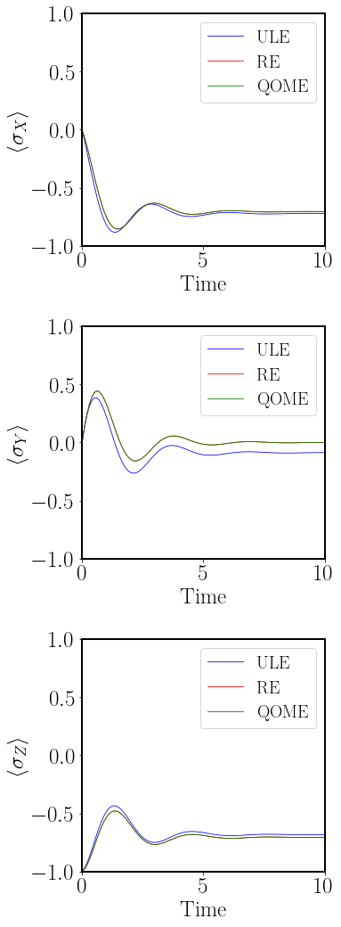
Figure 3: Comparison of the time dependent expectation values of the Pauli operators $\langle\hat{\sigma}_{i}\rangle$ after evolving a TLS coupled to a JC bath with the ULE, Redfield Equation (RE) and QOME respectively indicated in blue, red and green. Setting $E=1$, so that $t_{\text{final}}=10/E$, the parameters used to simulate the plotted evolution are as follows: $\alpha=0.2$, $T=0.05$, $\theta={\pi}/{2}$, $\phi={\pi}/{4}$, $\varphi={\pi}/{2}$, $\Omega=50$.

$$\mathcal{D}_{\text{UL-RE}}(t_{f})=T(\hat{\rho}_{\text{UL}}(t_{f}),\hat{\rho}_{\text{RE}}(t_{f}))$$ (56)

where the trace distance $T(\cdot)$ is defined as

$$T(\hat{\rho},\hat{\sigma})=\dfrac{1}{2}\Tr{\sqrt{(\hat{\rho}-\hat{\sigma})^{\dagger}(\hat{\rho}-\hat{\sigma})}}$$ (57)

see e.g. [2], and analogously we define

$$\mathcal{D}_{\text{QO-RE}}(t_{f})=T(\hat{\rho}_{\text{QO}}(t_{f}),\hat{\rho}_{\text{RE}}(t_{f})).$$ (58)

To compare the accuracy of the QOME and the UL with respect to the Redfield Equation, we pick 100 instances of the parameters $\phi$, $\theta$, $\varphi$, randomly defining the initial state and the mixing angle of the Hamiltonian, whitin the ranges in Table 1; and we sample 100 linearly spaced values for the coupling to the bath $\alpha$ and the temperature $T$ whitin the ranges in Table 2 the initial state $\rho(t=0)=\outerproduct{\psi_{0}}{\psi_{0}}$ is given by

$$\ket{\psi_{0}}=\cos{(\theta/2)}\ket{0}+e^{i\varphi}\sin{(\theta/2)\ket{1}}$$ (59)

and contains the random angles $\theta,\varphi$ while $\phi$ is the angle as in Eq. (53). The histograms in Fig. 4 show how many instances evolved with the ULE and the QOME end up having trace distance smaller than a certain threshold $\mathcal{D}_{\text{thres}}=0.01$. The height of the bars in the pair of plots on the left indicates the number of simulations for which $\mathcal{D}_{\text{UL-RE}}(t_{f})<\mathcal{D}_{\text{thres}}$; analogously, on the right are plotted the counts of density matrices evolved with the QOME satysfying $\mathcal{D}_{\text{UL-RE}}(t_{f})<\mathcal{D}_{\text{thres}}$. The type of bath does not seem to play a role since the upper pair, featuring an Ohmic spectral density function, looks pretty much the same as the bottom pair, where the spectral density function is JC. We notice that the accuracy of the QOME with respect to the Redfield Equation is on average much higher than that of the ULE. Only when the bath coupling $\alpha$ and temperature $T$ are much smaller than the qubit energy, so $E_{1}\gg\alpha,\,T$, the solutions become close in accuracy. In these cases, we expect coupling to the environment to be small enough that the effect of the Lindblad operators becomes negligible. Overall, this numerical analysis strongly indicates that the QOME surpasses the ULE in accuracy if the system-bath coupling is relevant.

Table 1: Random parameters of the TLS Hamiltonian and initial state

Parameters	Min. Value	Max. Value
$\phi$	0	$\pi/4$
$\theta$	0	$\pi$
$\varphi$	0	$2\pi$

Table 2: Linearly sampled coupling to the bath and temperature

Parameters	Min. Value	Max. Value
$\alpha$	0.1	$1$
$T$	0.01	0.1

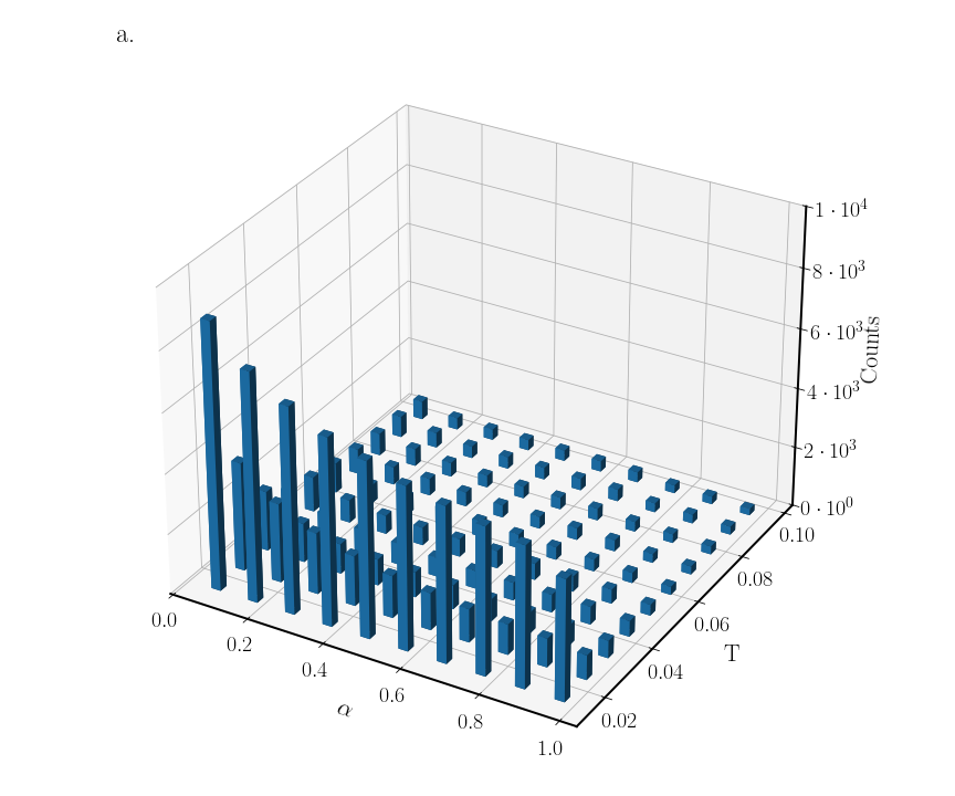
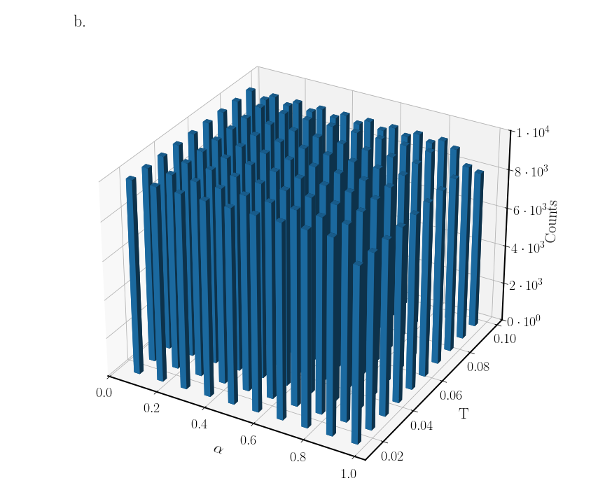
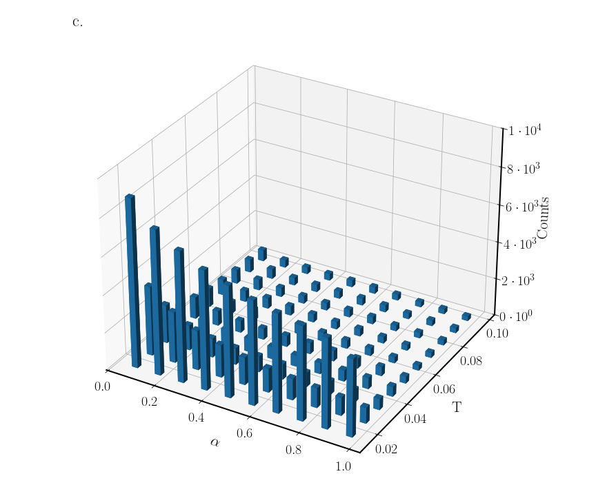
Figure 4: Histograms showing the number of instances whose final states (at a given time $t_{f}=10/E_{1}$) have a trace distance smaller than a certain value $\mathcal{D}_{\text{thres}}=0.01$ as a function of the coupling to the bath $\alpha$ and the temperature $T$. The parameters $\alpha$ and $T$ are linearly sampled within the intervals in Table 2, while the mixing angle and the Bloch sphere angles are randomly chosen within the ranges in Table 1. Plots a. and c.: $\mathcal{D}_{\text{UL-RE}}(t_{f})<0.01$ for an Ohmic and a JC bath respectively. Plots b. and d.: $\mathcal{D}_{\text{QO-RE}}(t_{f})<0.01$ for an Ohmic and a JC bath respectively.

IV Conclusions

In this work, we have shown a way to formally derive the Quantum Optical Master Equation from the Redfield Equation. This systematic way of deriving the QOME only needs to neglect terms of the same or higher order than those already neglected to derive the Redfield equation. The QOME therefore belongs to the same equivalence class of Markov approximations as the Redfield Equation. A similar procedure has already been done by Rudner and Nathan, who showed that the Universal Lindblad Equation also belongs to this equivalence class [1].

This result not only formally justifies the secular approximation that is usually done in a very informal way by just neglecting ”fast oscillating terms”, which in itself is of high analytical interest. Furthermore, analytical considerations hint that the QOME yields better results than the ULE.

To test this hypothesis, we applied both the Quantum Optical Master Equation and the Universal Lindblad Equation to solving single-qubit systems with varied parameters and comparing the solutions to the solution of the Redfield Equation. For the systems we considered, we found that on average, the Quantum Optical Master Equation yielded a result much closer to the solution of the Redfield equation. However, it remains an open question whether this is the case for other, more complex models. A natural continuation of this work would be to do numerical testing on more complex models to see if the QOME leads to more accurate results for those as well.

However, one caveat is that the QOME requires knowledge of the system eigenstates, while the ULE does not. A useful prospect for further work would be to see if the Lindblad operators of the Quantum Optical Master Equation can be derived without knowledge of the system eigenstates in a similar way as the Lindblad operator of the ULE can.

In conclusion, we have shown a formal way to derive the QOME from the Redfield Equation for any open quantum system. With that, we have shown that the QOME is of the same order of approximation than the Redfield equation, a result which is of great analytical and practical significance.