Some remarks on Frolov-AdS black hole surrounded by a fluid of strings

Abstract

A class of new solutions that generalizes the Frolov regular black hole solution is obtained. The generalization is performed by adding the cosmological constant and surrounding the black hole with a fluid of strings. Among these solutions, some preserve the regularity of the original Frolov solution, depending on the values of the parameter $\beta$ which labels the different solutions. A discussion is presented on the features of the solutions with respect to the existence or not of singularities, by examining the Kretschmann scalar, as well as, by analysing the behavior of the geodesics with respect to their completeness. It is performed some investigations concerning different aspects of thermodynamics, concerning the role played by the parameter associated to the Frolov regular black hole solution, as well as, of the parameter that codifies the presence of the fluid of strings. These are realized by considering diferent values of the parameter $\beta$, in particular, for $\beta=-1/2$, in which case the regularity of the Frolov black hole is preserved. All obtained results closely align with the ones obtained by taking the appropriate particularizations.

1 Introduction

The General Theory of Relativity predicts the existence of peculiar structures in the Universe which are called black holes. They remained an object of academic interest for a long time, since the discovery of a solution corresponding to a static and spherically symmetric black hole, by Schwarzschild [1] and its generalizations by Reissner and Nordström, with the inclusion of electric charge [2, 3] and by Kerr and Newman who considered the rotation [4, 5]. It is worth calling attention to the fact that all spacetimes associated with these solutions have singularities, in which the curvature diverges and the General Theory of Relativity breaks down. Therefore, the existence of these singular solutions may represent a failure of the theory, which must be corrected, certainly, by constructing a quantum theory of gravity [6].

A more direct way to avoid singularities is to construct some models of black holes without spacetime singularities, namely, black holes having regular centers, which are called regular black holes or nonsingular black holes.

A class of black holes without a singularity, namely, regular or non-singular black holes was constructed by Bardeen [7], using phenomenological assumptions, which results a metric representing a simple redefinition of the mass in the Schwarzschild solution, now depending on the radial coordinate. Inspired by the solution obtained by Bardeen [7], in the sequence, different regular black hole solutios have been obtained in the literature [8, 9, 10, 11, 12, 13, 14, 15]. The properties of regular black holes were also studied, as, for example, the black hole thermodynamics [16, 17, 18, 19], geodesics [20, 21] and quasinormal modes [22, 23, 24, 25].

Among the regular spacetimes, in this work, we will focus on the Frolov metric [13], which represents a static and spherically symmetric black hole that behaves like a de Sitter spacetime at the origin ($r\rightarrow 0$) and is asymptotically Reissner-Nordström for $r\rightarrow\infty$. The Frolov solution presents an additional charge parameter as compared with Hayward black hole [15] solution and can be understood as a kind of generalization of this one. It can also be understood as an exact model of a black hole in the General Theory of Relativity coupled with nonlinear electrodynamics.

Forty five years ago, Letelier construed a gauge-invariant model of a cloud of strings [26], motivated by the idea that the fundamental building blocks of of nature are one-dimensional objects, namely, stings, rather than point particles. Two years later, Letelier generalized the original model, including the pressure. In this context, instead of a cloud of strings, we have a fluid of strings [27]. The solution corresponding to a static black hole immersed in this fluid of strings was obtained by Soleng [28], who argued that this model, in principle, can be used to explain the rotation curves of galaxies.

One of the most important moments in the history of cosmology was the discovery of the fact that the Universe experiences an accelerated expansion [29, 30, 31]. From this accelerated expansion, we can infer that on a large scale, there is a repulsive energy that causes a negative pressure. Several mathematical models have been proposed to explain this accelerated phenomenon, among them, the one based on the cosmological constant [32]. In the context of astrophysics, the cosmological constant has also been associated with a thermodynamic pressure in black hole systems, which leads to very interesting consequences [33, 34].

Since the pioneering studies of Bekenstein and Hawking in the 1970s [35, 36, 37], the thermodynamics of black holes has been studied, motivated mainly by the belief that it can connect gravity and quantum mechanics. In these studies, the presence of a cosmological constant has an important role, since, as already mentioned, it can be interpreted as a thermodynamic pressure with a conjugated thermodynamic volume associated with it [33]. Thus, it is possible to study the black hole system using various thermodynamic potentials and calculate the corresponding intensive variables, and additionally to analyze the black hole stability and phase transitions.

In this paper, we obtain a class of solutions that correspond to a generalization of the Frolov black hole solution [13], in the sense that due to the presence of the cosmological constant, which gives rise to an AdS term, and a fluid of strings. The resulting spacetime we are calling Frolov-AdS black hole surrounded by a fluid of strings. In this scenario, a class of spacetimes is obtained, corresponding to different values of the parameter $\beta$, which codifies the different solutions.

It is worth calling attention to the fact that the particular solution we have obtained, namely, $\beta=2$, was considered in the literature as a possible solution that can mimic a perfect fluid dark matter [28, 38]. We perform a detailed study of the black hole thermodynamics, analyzing the system stability and phase transitions.

This paper is organized as follows. In Sec. 2, we obtain a class of solutions corresponding to the Frolov-AdS black hole surrounded by a fluid of string, behavior, calculate and discuss the results related to the Kretschmann scalar, and analyse the geodesics concerning their completeness or incompleteness. In. Sec. 3, we study some aspects of the thermodynamics of black holes, with emphasis on the behavior of some thermodynamic quantities in which concerns their dependence on the intensity of the fluid of strings. Finally, in Sec. 4, we present our concluding remarks.

2 Frolov-AdS black hole surrounded by a fluid of strings.

2.1 Introduction

Let us start by considering the Frolov black hole spacetime [13] which can be obtained as a solution of Einstein’s equation coupled to a nonlinear electromagnetic field. Thus, taking this solution as a seed, we include the cosmological constant and a fluid of strings surrounding this black hole, and obtain a class of spherically symmetric solutions that generalizes the one obtained by Frolov[13].

Firstly, let us write the action that describes the system under consideration, taking into account a minimally coupled nonlinear electromagnetic field, given by

$$S=\frac{1}{16\pi}\int d^{4}x\sqrt{-g}(R+\mathcal{L}),$$ (1)

with $g$ being the determinant of the metric tensor, $g_{\mu\nu}$, $R$ the scalar curvature and $\mathcal{L}$ the Lagrangian density associated to the nonlinear electromagnetic field [39].

Performing the variation of the action given by Eq.(1), with respect to the metric, we find the equations [40]

$$G_{\mu\nu}=2\left(\frac{\partial\mathcal{L}(F)}{\partial F}F_{\mu\sigma}F^{\sigma}_{\,\,\nu}-\frac{1}{4}g_{\mu\nu}\mathcal{L}(F)\right),$$ (2)

where $G_{\mu\nu}=R_{\mu\nu}-\frac{1}{2}Rg_{\mu\nu}$. In which concerns the nonlinear electromagnetic field, the equations that should be obeyed are the following:

$$\nabla_{\mu}\left(\frac{\partial\mathcal{L}(F)}{\partial F}F^{\nu\mu}\right)=0,$$ (3)

$$\nabla_{\mu}(*F^{\nu\mu})=0,$$ (4)

where $F_{\mu\nu}=2\nabla_{[\mu}A_{\nu]}$ is the nonlinear electromagnetic field, with $A_{\mu}$ being the potential, and $\mathcal{L}$ is a function of $F=\frac{1}{4}F_{\mu\nu}F^{\mu\nu}$.

The metric of the non-singular (regular) black hole obtained by Frolov [13] is given by

$$ds^{2}=f(r)dt^{2}-f(r)^{-1}dr^{2}-r^{2}d\Omega^{2},$$ (5)

where $d\Omega^{2}=d\theta^{2}+\sin^{2}\theta d\phi^{2}$. The function $f(r)$ is given by

$$f(r)=1-\frac{r^{2}\left(2mr-Q^{2}\right)}{l^{2}\left(2mr+Q^{2}\right)+r^{4}},$$ (6)

where the additional charge parameter $Q$ characterizes a specific hair and satisfies $0<Q\leq 1$ and the length below which quantum gravity effects become important satisfies, $l\leq\sqrt{16/27}$ as in the case of the Hayward black hole [15, 41]. In principle, $Q$ admits an interpretation in terms of electric charge measured by an observer situated at infinity, where the metric is asymptotically flat [42]. In the limit $l\rightarrow 0$, this metric reproduces the Reissner-Nordström metric [2].

Using the metric given by Eq. (6), we can obtain the following components of the Einstein tensor:

$$G_{t}^{\;t}=G_{r}^{\;r}=\frac{l^{2}\left(12m^{2}r^{2}+4mQ^{2}r-3Q^{4}\right)+Q^{2}r^{4}}{\left(l^{2}\left(2mr+Q^{2}\right)+r^{4}\right)^{2}},$$ (7)

$$G_{\theta}^{\;\theta}=G_{\phi}^{\;\phi}= \frac{24l^{2}m^{2}r^{3}\left(l^{2}m-r^{3}\right)}{\left(l^{2}\left(2mr+Q^{2}\right)+r^{4}\right)^{3}}+\frac{6l^{2}Q^{4}r\left(l^{2}m+2r^{3}\right)}{\left(l^{2}\left(2mr+Q^{2}\right)+r^{4}\right)^{3}}$$ (8)

$$-\frac{Q^{2}\left(l^{4}\left(3Q^{4}-28m^{2}r^{2}\right)+6l^{2}mr^{5}+r^{8}\right)}{\left(l^{2}\left(2mr+Q^{2}\right)+r^{4}\right)^{3}},$$

which, according to Einstein’s equations, are proportional to the energy-momentum tensor of the source.

Now, let us generalize the metric obtained by Frolov [13], given by Eqs.(6), taking into account the cosmological constant and the fluid of strings. To do this, we add the term $-\Lambda g_{\mu\nu}$ and the energy momentum tensor corresponding to the fluid of strings to the lhs and rhs, respectively of Eq. (2). Thus, we can write

$$R_{\mu\nu}-\frac{1}{2}Rg_{\mu\nu}-\Lambda g_{\mu\nu}=2\left(\frac{\partial\mathcal{L}(F)}{\partial F}F_{\mu\sigma}F^{\sigma}_{\,\,\nu}-\frac{1}{4}g_{\mu\nu}\mathcal{L}(F)\right)+T_{\mu\nu}^{\text{FS}},$$ (9)

where $T_{\mu\nu}^{\text{FS}}$ refers to the energy-momentum tensor of the fluid of strings. Therefore, the contents of the rhs represent an effective energy-momentum tensor, with the first arising from the nonlinear electromagnetic field, while the second refers to the fluid of strings.

2.2 Energy-momentum tensor of a fluid of strings

The trajectory of a particle which moves with a four-velocity $u^{\mu}=dx^{\mu}/d\lambda$, where $\lambda$ is a parameter, can be described by the curve $x=x(\lambda)$. In the case of a moving infinitesimally thin string, the trajectory corresponds to a two-dimensional world sheet described by [43]

$$x^{\mu}=x^{\mu}(\lambda^{a}),\;\;a=0,1,$$ (10)

with $\lambda_{0}$ and $\lambda_{1}$ being timelike and spacelike parameters, respectively. We can associate with this world sheet, a bivector $\Sigma^{\mu\nu}$, given by [43]

$$\Sigma^{\mu\nu}=\epsilon^{ab}\frac{\partial{x^{\mu}}}{\partial{\lambda^{a}}}\frac{\partial{x^{\nu}}}{\partial{\lambda^{b}}},$$ (11)

where $\epsilon^{ab}$ is the two-dimensional Levi-Civita symbol, in which the following values will be considered: $\epsilon^{01}=-\epsilon^{10}=1$.

It is worth emphasizing that on this world sheet, there will be an induced metric, $\gamma_{ab}$, with $a,b=0,1$, such that,

$$\gamma_{ab}=g_{\mu\nu}\frac{\partial{x^{\mu}}}{\partial{\lambda^{a}}}\frac{\partial{x^{\nu}}}{\partial{\lambda^{b}}},$$ (12)

whose determinant is denoted by $\gamma$.

The energy-momentum tensor associated with a dust cloud is given by $T^{\mu\nu}=\rho u^{\mu}u^{\nu}$, with $u^{\mu}$ being the normalized four-velocity of a dust particle and $\rho$ the proper density of the flow. Analogously, for a cloud of strings, the energy-momentum tensor can be defined as [43]

$$T^{\mu\nu}=\rho\frac{\Sigma^{\mu\beta}\Sigma_{\beta}^{\;\nu}}{(-\gamma)^{1/2}},$$ (13)

where $\gamma=\frac{1}{2}\Sigma^{\mu\nu}\Sigma_{\mu\nu}$.

Let us consider a more general case, taking into account the pressure of a fluid of strings. This scenario corresponds to a perfect fluid of strings with pressure $p$, whose energy-momentum tensor is given by [44]

$$T^{\mu\nu}=(p+\sqrt{-\gamma}\rho)\frac{\Sigma^{\mu\beta}\Sigma_{\beta}^{\;\nu}}{(-\gamma)}+pq^{\mu\nu}.$$ (14)

Taking into account the energy-momentum tensor given by Eq. (14), it was obtained the metric corresponding to a static black hole surrounded by a fluid of strings [45]. In this context, it was assumed that the components of the energy-momentum tensor are related through the equations

$$T_{t}^{\;t}=T_{r}^{\;r},$$ (15)

$$T_{t}^{\;t}=-\beta T_{\theta}^{\;\theta}=-\beta T_{\phi}^{\;\phi},$$ (16)

where $\beta$ is a dimensionless constant. The energy-momentum tensor, whose components are given by Eqs. (15)-(16), was interpreted as being associated with a kind of anisotropic fluid with spherical symmetry [8, 46].

It is worth calling attention to the fact that this kind of energy-momentum tensor has been used in different scenarios [47, 48, 49]. In particular, in Ref. [47] it is shown that the conditions imposed by Eq. (16) permit to obtaining of a class of spherically symmetric solutions of Einstein’s field equations with two parameters.

In this paper, we will consider the components of the energy-momentum tensor for the fluid of strings obtained in [50] and already used in a previous paper[51]. These components are given by [50]

$$T_{t}^{\;t}=T_{r}^{\;r}=-\frac{\epsilon}{r^{2}}\left(\frac{b}{r}\right)^{2/\beta},$$ (17)

$$T_{\theta}^{\;\theta}=T_{\phi}^{\;\phi}=\frac{\epsilon}{\beta r^{2}}\left(\frac{b}{r}\right)^{2/\beta},$$ (18)

where $b$ is a positive integration constant and $\epsilon=\pm 1$, with the $\pm$ referring to the signs of the energy density of the fluid of strings.

2.3 Frolov black hole solution with cosmological constant and surrounded by a fluid of strings

Now, let us consider Eq. (9) with the components of the energy-momentum tensor of the fluid of strings given by Eqs. (17) and (18).

The line element for a static and spherically symmetric spacetime can be written as:

$$ds^{2}=e^{\nu(r)}dt^{2}-e^{\lambda(r)}dr^{2}-r^{2}d\theta^{2}-r^{2}\sin^{2}\theta d\phi^{2}.$$ (19)

Einstein’s field equations for the present case, in which the presence of the cosmological constant and of the fluid of strings are taken into account, can be written as

$$e^{-\lambda}\left(\frac{\lambda^{\prime}}{r}-\frac{1}{r^{2}}\right)+\frac{1}{r^{2}}-\Lambda=\frac{l^{2}\left(12m^{2}r^{2}+4mQ^{2}r-3Q^{4}\right)+Q^{2}r^{4}}{\left(l^{2}\left(2mr+Q^{2}\right)+r^{4}\right)^{2}}-\frac{\epsilon}{r^{2}}\left(\frac{b}{r}\right)^{2/\beta},$$ (20)

$$-e^{-\lambda}\left(\frac{\nu^{\prime}}{r}+\frac{1}{r^{2}}\right)+\frac{1}{r^{2}}-\Lambda=\frac{l^{2}\left(12m^{2}r^{2}+4mQ^{2}r-3Q^{4}\right)+Q^{2}r^{4}}{\left(l^{2}\left(2mr+Q^{2}\right)+r^{4}\right)^{2}}-\frac{\epsilon}{r^{2}}\left(\frac{b}{r}\right)^{2/\beta},$$ (21)

$$\frac{1}{2}e^{-\lambda}\left(\frac{\nu^{\prime}\lambda^{\prime}}{2}+\frac{\lambda^{\prime}}{r}-\frac{\nu^{\prime}}{r}-\frac{\nu^{\prime 2}}{2}-\nu^{\prime\prime}\right)-\Lambda= +\frac{24l^{2}m^{2}r^{3}\left(l^{2}m-r^{3}\right)}{\left(l^{2}\left(2mr+Q^{2}\right)+r^{4}\right)^{3}}$$ (22)

$$+\frac{6l^{2}Q^{4}r\left(l^{2}m+2r^{3}\right)}{\left(l^{2}\left(2mr+Q^{2}\right)+r^{4}\right)^{3}}$$

$$-\frac{Q^{2}\left(l^{4}\left(3Q^{4}-28m^{2}r^{2}\right)+6l^{2}mr^{5}+r^{8}\right)}{\left(l^{2}\left(2mr+Q^{2}\right)+r^{4}\right)^{3}}$$

$$+\frac{\epsilon}{\beta r^{2}}\left(\frac{b}{r}\right)^{2/\beta}.$$

From Eqs. (20) and (21), it follows immediately that:

$$\nu=-\lambda+const.$$ (23)

The constant can be absorbed into a rescaling of the time coordinate, so that,

$$\nu=-\lambda.$$ (24)

Adding Eqs. (20) and (21) and considering Eq. (24), after some algebraic manipulations, we obtain:

$$e^{-\lambda}\frac{\lambda^{\prime}}{r}-e^{-\lambda}\frac{1}{r^{2}}+\frac{1}{r^{2}}-\Lambda=\frac{l^{2}\left(12m^{2}r^{2}+4mQ^{2}r-3Q^{4}\right)+Q^{2}r^{4}}{\left(l^{2}\left(2mr+Q^{2}\right)+r^{4}\right)^{2}}-\frac{\epsilon}{r^{2}}\left(\frac{b}{r}\right)^{2/\beta}.$$ (25)

Then, consider an arbitrary function $f(r)$, such that

$$\nu=-\lambda=ln(1+f(r)).$$ (26)

Taking Eqs. (24) and (26) into account, we can write Eqs. (25) and (22) and, respectively, as follows:

$$-\frac{1}{r^{2}}(rf^{\prime}+f)-\Lambda=\frac{l^{2}\left(12m^{2}r^{2}+4mQ^{2}r-3Q^{4}\right)+Q^{2}r^{4}}{\left(l^{2}\left(2mr+Q^{2}\right)+r^{4}\right)^{2}}-\frac{\epsilon}{r^{2}}\left(\frac{b}{r}\right)^{2/\beta},$$ (27)

$$2\frac{f^{\prime}}{r}+f^{\prime\prime}+2\Lambda= -\frac{48l^{2}m^{2}r^{3}\left(l^{2}m-r^{3}\right)}{\left(l^{2}\left(2mr+Q^{2}\right)+r^{4}\right)^{3}}$$ (28)

$$-\frac{12l^{2}Q^{4}r\left(l^{2}m+2r^{3}\right)}{\left(l^{2}\left(2mr+Q^{2}\right)+r^{4}\right)^{3}}$$

$$+\frac{2Q^{2}\left(l^{4}\left(3Q^{4}-28m^{2}r^{2}\right)+6l^{2}mr^{5}+r^{8}\right)}{\left(l^{2}\left(2mr+Q^{2}\right)+r^{4}\right)^{3}}$$

$$-\frac{2\epsilon}{\beta r^{2}}\left(\frac{b}{r}\right)^{2/\beta}.$$

Multiplying both Eqs. (27) and (28) by $r^{2}$ and adding the obtained equations, we get the following differential equation:

$$r^{2}f^{\prime\prime}+rf^{\prime}-f+\Lambda r^{2}+\epsilon\left(\frac{\beta+2}{\beta}\right)\left(\frac{b}{r}\right)^{2/\beta}$$ (29)

$$-\frac{l^{2}r^{2}\left(12m^{2}r^{2}+4mQ^{2}r-3Q^{4}\right)+Q^{2}r^{6}}{\left(l^{2}\left(2mr+Q^{2}\right)+r^{4}\right)^{2}}$$

$$+\frac{48l^{2}m^{2}r^{5}\left(l^{2}m-r^{3}\right)}{\left(l^{2}\left(2mr+Q^{2}\right)+r^{4}\right)^{3}}+\frac{12l^{2}Q^{4}r^{3}\left(l^{2}m+2r^{3}\right)}{\left(l^{2}\left(2mr+Q^{2}\right)+r^{4}\right)^{3}}$$

$$-\frac{2Q^{2}r^{2}\left(l^{4}\left(3Q^{4}-28m^{2}r^{2}\right)+6l^{2}mr^{5}+r^{8}\right)}{\left(l^{2}\left(2mr+Q^{2}\right)+r^{4}\right)^{3}}=0,$$

whose solution is given by:

$$f(r)=-\frac{r^{2}\left(2mr-Q^{2}\right)}{l^{2}\left(2mr+Q^{2}\right)+r^{4}}-\frac{\Lambda r^{2}}{3}+\left\{\begin{array}[]{rcl}\epsilon b[1+2\log(r)]/2r\text{ for }\beta=2,\\ \epsilon\beta(\beta-2)^{-1}\left(\frac{b}{r}\right)^{2/\beta}\text{ for }\beta\neq 2.\end{array}\right.$$ (30)

So, substitute Eq. (30) into Eq. (26) and then into Eq. (19), we finally obtain the Frolov-AdS black hole surrounded by a fluid of strings, where the line element can be written as

$$ds^{2}=f(r)dt^{2}-f(r)^{-1}dr^{2}-r^{2}d\Omega^{2},$$ (31)

where $d\Omega^{2}=d\theta^{2}+\sin^{2}\theta d\phi^{2}$. The function $f(r)$ is given by:

$$f(r)=1-\frac{r^{2}\left(2mr-Q^{2}\right)}{l^{2}\left(2mr+Q^{2}\right)+r^{4}}-\frac{\Lambda r^{2}}{3}+\left\{\begin{array}[]{rcl}\epsilon b[1+2\log(r)]/2r\text{ for }\beta=2,\\ \epsilon\beta(\beta-2)^{-1}\left(\frac{b}{r}\right)^{2/\beta}\text{ for }\beta\neq 2.\end{array}\right.$$ (32)

Note that we can recover some other solutions from this metric if we make the choices displayed in the Table (1).

Table 1: Special cases for $l=Q=\Lambda=0$.

$\epsilon$				$b$				$\beta$				Spacetime
$1$				$\mathbb{R}^{*}$				$lim_{\beta\rightarrow\infty}$				Letelier
$1$				$Q$				$1$				Reissner-Nordström
$1$				$\Lambda^{-1/2}$				$-1$				de Sitter

Note that the class of solutions obtained can be considered as sourced by two fluids, namely, one corresponding to the fluid of strings and the other to a nonlinear electromagnetic field. In addition, a cosmological constant is considered.

2.4 The Kretschmann scalar: calculation and discussion

Now, let us discuss the existence of physical singularities of spacetime by considering one of the scalars constructed with the curvature tensor, namely the Kretschmann scalar. It is worth pointing out that the absence of singularities in such a curvature scalar does not guarantee that the spacetime is regular. The discussions will be compared with similar ones for a Frolov black hole, which is regular. In the section that follows, we will analyze the same question, but this time, taking into account the geodesics [52, 53].

In what follows, we will determine and analyze the limits of the Kretschmann scalar when $r\rightarrow 0$ and $r\rightarrow\infty$, for $l>0$, $Q>0$, $b>0$ and $\Lambda$ and $\epsilon\in\mathbb{R}$, for some values of $\beta$.

• For $\beta=-2$, the Kretschmann scalar diverges very close to the origin and is finite in a region very far from the black hole.

  $$\lim_{r\rightarrow 0}K=\infty.$$ (33)

  $$\lim_{r\rightarrow\infty}K=\frac{8\Lambda^{2}}{3}.$$ (34)

• For $\beta=-1$, the Kretschmann scalar is finite, and is given by

  $$\lim_{r\rightarrow 0}K=\frac{8\left(b^{2}\left(3-\Lambda l^{2}\right)+l^{2}\epsilon\right)^{2}}{3b^{4}l^{4}}.$$ (35)

  $$\lim_{r\rightarrow\infty}K=\frac{8\left(\epsilon-b^{2}\Lambda\right)^{2}}{3b^{4}}.$$ (36)

• For $-1<\beta<0$, the Kretschmann scalar is finite, close to the origin, and diverges for points very far from the black hole, according to

  $$\lim_{r\rightarrow 0}K=\frac{8\left(\Lambda l^{2}-3\right)^{2}}{3l^{4}}.$$ (37)

  $$\lim_{r\rightarrow\infty}K=\infty.$$ (38)

• For $\beta=1$, $\beta=2$ and $\beta=3$, the Kretschmann scalar diverges very close to the origin and has a finite value for points very far from the black hole.

  $$\lim_{r\rightarrow 0}K=\infty.$$ (39)

  $$\lim_{r\rightarrow\infty}K=\frac{8\Lambda^{2}}{3}.$$ (40)

These results tell us that the inclusion of the fluid of strings changes the regularity of the Frolov solution for the following values of $\beta$, such that $\beta<-1$ and $\beta>0$. Otherwise, the regularity of the Frolov black hole solution is preserved in the interval $-1\leq\beta<0$.

2.5 Geodesics and Effective Potential

Let us now consider the static and spherically symmetric solution given by Eq. (32) and analyze the geodesic equations. To do this, consider the Lagrangian $\mathcal{L}$, such that

$$2\mathcal{L}=f(r)\dot{t}^{2}-\frac{1}{f(r)}\dot{r}^{2}-r^{2}\dot{\theta}^{2}-r^{2}\sin^{2}\theta\dot{\phi}^{2}.$$ (41)

The “point” represents the derivative concerning proper time, $\tau$. For simplicity, let’s restrict the analysis of the geodesics to the equatorial plane of the black hole, $\theta=\frac{\pi}{2}$. Using the Euler-Lagrange equations, we obtain

$$E =f(r)\dot{t},$$ (42)

$$J =-r^{2}\dot{\phi},$$ (43)

where $E$ and $J$ are constants of motion. which can be interpreted as the energy $E$ and the angular momentum $J$ of the particle moving around the black hole.

By rescaling the parameter $\tau$, we can define $L=2\mathcal{L}$, which, for time-like geodesics, is equal to $+1$, for space-like geodesics is equal to $-1$, and is equal to $0$ for null geodesics [54]. Substituting Eqs. (42) and (43) into Eq. (41), we get

$$\dot{r}^{2}=E^{2}-V_{eff},$$ (44)

where

$$V_{eff}=f(r)\left(\frac{J^{2}}{r^{2}}+L\right).$$ (45)

Let’s now consider the problem of the massive particle $(L=1)$ falling radially $(J=0)$ into the black hole. The equation of radial geodesic motion of this test particle is given by

$$\dot{r}^{2}=E^{2}-f(r),$$ (46)

while the effective potential is as follows

$$V_{eff}=f(r).$$ (47)

The graphs for $\dot{r}^{2}$ and $V_{eff}$ are shown in Fig. 1.

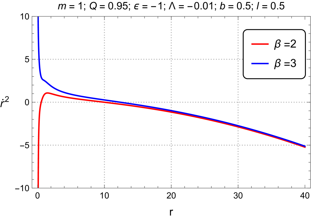
(a)

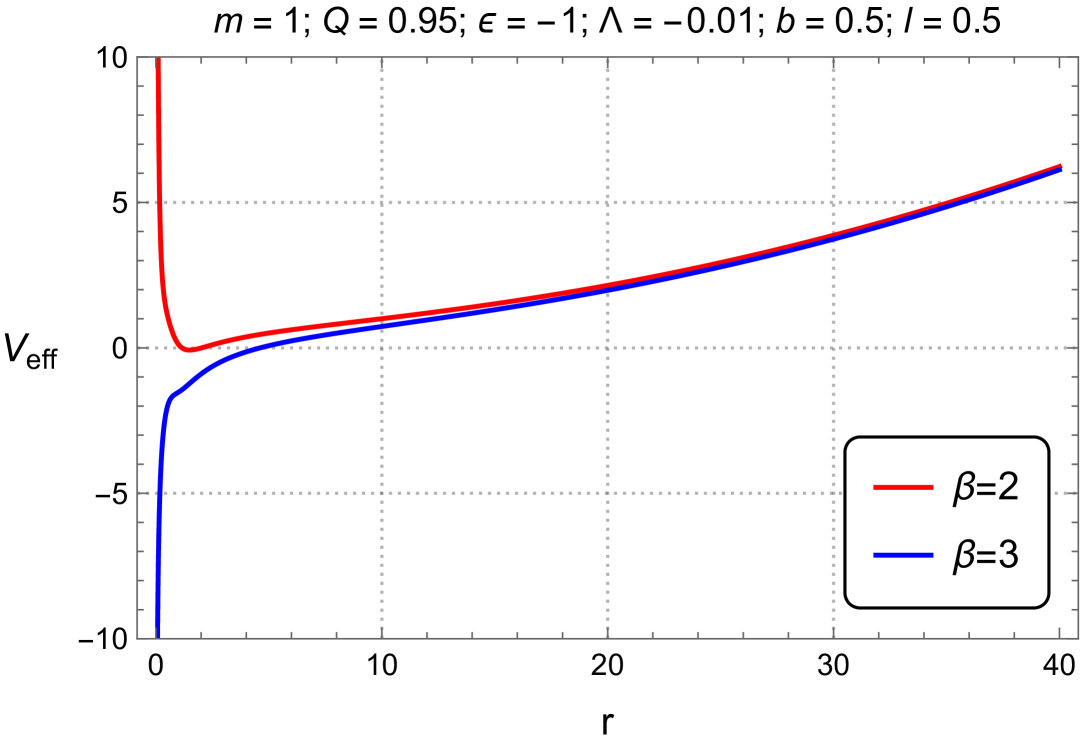
(b)

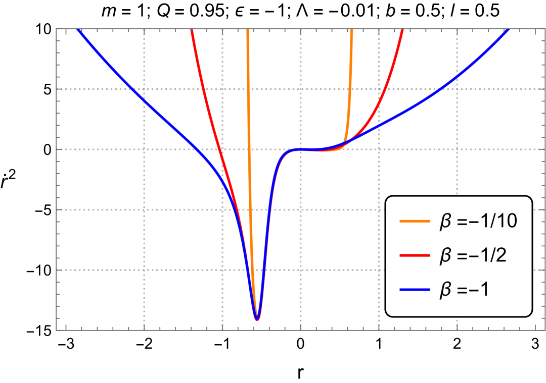
(c)

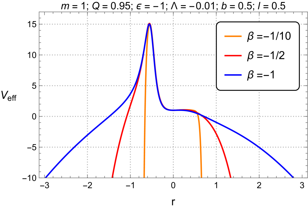
(d)

Figure 1: The graph on the left shows $\dot{r}^{2}$ for $E=2$. The graph on the right shows the effective potential $V_{eff}=f(r)$.

Let’s now compare the results predicted by the values of the Kretschmann scalar when $r\rightarrow 0$, with the characteristics of the geodesics, namely whether they are complete or incomplete.

In Fig. 1(b), we can conclude that the particle cannot reach the point $r=0$ in a finite time, for both values of $\beta$, namely, $\beta=2$ and $\beta=3$. This indicates that the geodesics are incomplete and therefore space-time is singular. This conclusion is confirmed by the fact that, for $\beta=2$, the Kretschmann scalar is infinite when $r\rightarrow 0$.

For $\beta=-1/10$, $\beta=-1/2$ and $\beta=-1$ in Fig. 1(d), the test particle manages to cross the potential barrier and reach the point $r=0$ in a finite time. This indicates that the geodesics are complete and therefore space-time is regular.

In summary, the analysis of the geodesics to know the characteristics of the spacetimes in relation to the singularity confirms what is predicted by the results provided by the Kretschmann scalar, at least in the cases considered.

3 Black Hole Thermodynamics

In this section, we will study the thermodynamics of the Frolov-AdS black hole with a fluid of strings, examining the behavior of mass, Hawking temperature, and heat capacity as a function of entropy.

It is worth calling attention to two considerations that we will assume in this work:

(i) We will study the solution $\beta=2$ since this choice may represent the presence of dark matter [28];

(ii) We will also analyze thermodynamics for values of $-1\leq\beta<0$, since in this interval we obtain regular solutions, preserving the main characteristic of the Frolov solution, namely regularity.

3.1 Black hole mass

Let $r_{h}$ be the radius of the horizon, so we have $f(r_{h})=0$, where $f(r)$ is given by Eq. (32). So we can write the mass of the black hole in terms of $r_{h}$ using the following equation:

$$m^{(\beta=2)}=\frac{l^{2}Q^{2}\left(3b\epsilon-2\Lambda r_{h}^{3}+6r_{h}\right)+6b\epsilon\log\left(r_{h}\right)\left(r_{h}^{4}+l^{2}Q^{2}\right)+r_{h}^{3}\left(3b\epsilon r_{h}-2\Lambda r_{h}^{4}+6r_{h}^{2}+6Q^{2}\right)}{2r_{h}\left(l^{2}\left(-3b\epsilon+2\Lambda r_{h}^{3}-6r_{h}\right)-6bl^{2}\epsilon\log\left(r_{h}\right)+6r_{h}^{3}\right)},$$ (48)

$$m^{(\beta\neq 2)}=\frac{3\beta\epsilon\left(\frac{b}{r_{h}}\right){}^{2/\beta}\left(r_{h}^{4}+l^{2}Q^{2}\right)+(\beta-2)\left(l^{2}Q^{2}\left(3-\Lambda r_{h}^{2}\right)+3r_{h}^{2}\left(r_{h}^{2}+Q^{2}\right)-\Lambda r_{h}^{6}\right)}{2l^{2}r_{h}\left((\beta-2)\left(\Lambda r_{h}^{2}-3\right)-3\beta\epsilon\left(\frac{b}{r_{h}}\right){}^{2/\beta}\right)+6(\beta-2)r_{h}^{3}},$$ (49)

written in terms of the parameter that describes the presence of the fluid of strings, $b$. Note that if $b=0$, we recover the mass of the regular Frolov-AdS black hole, without the fluid of strings, in terms of the radius of the horizon. Considering $l=0$, $\Lambda=0$ and $b=0$, we recover the mass of the Reissner-Nordström black hole.

The expression for the mass parameter can be rewritten in terms of the entropy, by using the following relation [35]

$$S=\frac{A}{4}=\pi r_{h}^{2},$$ (50)

as follows

$$m^{(\beta=2)}= [\pi^{2}l^{2}Q^{2}\left(-3\pi^{3/2}b\epsilon+2\Lambda S^{3/2}-6\pi\sqrt{S}\right)$$ (51)

$$+S^{3/2}\left(-3\pi^{3/2}b\sqrt{S}\epsilon-6\pi^{2}Q^{2}+2\Lambda S^{2}-6\pi S\right)$$

$$-3\pi^{3/2}b\epsilon\log\left(\frac{S}{\pi}\right)\left(\pi^{2}l^{2}Q^{2}+S^{2}\right)]/$$

$$[2\pi^{3/2}\sqrt{S}\left(l^{2}\left(3\pi^{3/2}b\epsilon-2\Lambda S^{3/2}+6\pi\sqrt{S}\right)+3\pi^{3/2}bl^{2}\epsilon\log\left(\frac{S}{\pi}\right)-6S^{3/2}\right)],$$

$$m^{(\beta\neq 2)}=\frac{3\pi^{1/\beta}\beta\epsilon\left(\frac{b}{\sqrt{S}}\right)^{2/\beta}\left(l^{2}Q^{2}+\frac{S^{2}}{\pi^{2}}\right)+(\beta-2)\left(l^{2}Q^{2}\left(3-\frac{\Lambda S}{\pi}\right)+\frac{3S\left(Q^{2}+\frac{S}{\pi}\right)}{\pi}-\frac{\Lambda S^{3}}{\pi^{3}}\right)}{\frac{2l^{2}\sqrt{S}\left((\beta-2)\left(\frac{\Lambda S}{\pi}-3\right)-3\pi^{1/\beta}\beta\epsilon\left(\frac{b}{\sqrt{S}}\right)^{2/\beta}\right)}{\sqrt{\pi}}+\frac{6(\beta-2)S^{3/2}}{\pi^{3/2}}}.$$ (52)

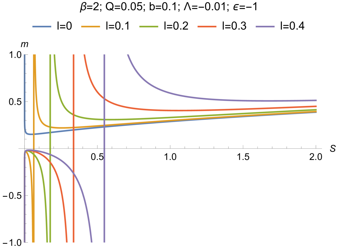
(a)

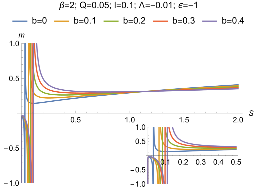
(b)

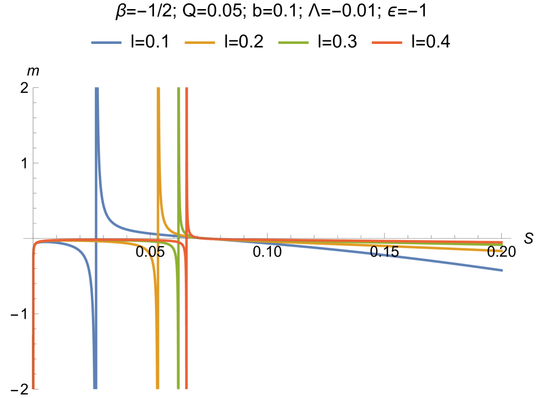
(c)

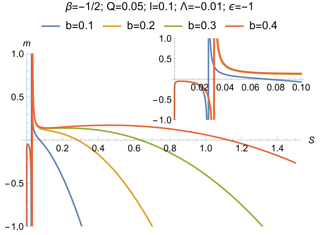
(d)

Figure 2: Black hole mass as a function of entropy $m(S)$ for different values of $b$ and $l$.

In Figs. 2(a)-2(d), we represent the behavior of the mass parameter, $m$, as a function of the entropy of the black hole, $S$, in different situations. Note that Figs. 2(a)-2(b), describe the behavior of mass as a function of entropy for the singular Frolov-AdS spacetime with dark matter fluid ($\beta=2$), while Figs. 2(c)-2(d), describe the mass as a function of entropy for the regular Frolov-AdS spacetime with fluid of strings for $\beta=-1/2$. Note also that, for the Frolov-AdS black hole with fluid of strings ($\beta=2$ and $\beta=-1/2$), the mass parameter has positive and negative values depending on the parameters of the black hole.

It is worth emphasizing that Figs. 2(a)-2(b) have the same limits, so that the mass will show positive values as the entropy takes on increasing values. If we set $S=2$ in Figs. 2(a)-2(b), we can see that the mass increases as $l$ increases and $b$ decreases. In Figs. 2(c)-2(d), the limits are the same, but opposite to those found in Figs. 2(a)-2(b). If we set $S=0.2$ in Figs. 2(c)-2(d), we conclude that the mass increases as we increase the values of $l$ and $b$.

3.2 Hawking temperature

Firstly, let us calculate the surface gravity, $\kappa$, for the space-timesunder consideration, defined as:

$$\kappa=\frac{f^{\prime}(r)}{2}\left|\frac{}{}_{r_{h}}\right.,$$ (53)

where $(^{\prime})$ means the derivative concerning the radial coordinate. Using surface gravity, the Hawking temperature for a stationary space-time is given by [55]:

$$T_{\kappa}=\frac{\kappa}{2\pi}.$$ (54)

Now, consider $f(r)$ given by Eq.(32) and substitute into Eqs. (53) and (54). Thus, the Hawking temperature, $T_{\kappa}=T$, for the Frolov-AdS black hole with a fluid of strings can be written as:

$$T^{(\beta=2)}= \frac{1}{144\pi^{7/2}S^{5/2}\left(2l^{2}Q^{2}+\frac{S^{2}}{\pi^{2}}\right)}\left[36\pi^{4}l^{4}Q^{2}S-12\Lambda S^{5}\left(\Lambda l^{2}+3\right)+36\pi S^{4}\left(2\Lambda l^{2}+1\right)\right.$$ (55)

$$\left.+4\pi^{2}S^{3}\left(\Lambda^{2}l^{4}Q^{2}-27l^{2}-9Q^{2}\right)+36\pi^{3/2}bS^{7/2}\epsilon\left(\Lambda l^{2}+2\Lambda l^{2}\log\left(\frac{\sqrt{S}}{\sqrt{\pi}}\right)+1\right)\right.$$

$$\left.-12\pi^{7/2}bl^{2}Q^{2}S^{3/2}\epsilon\left(\Lambda l^{2}+2\left(\Lambda l^{2}+9\right)\log\left(\frac{\sqrt{S}}{\sqrt{\pi}}\right)+3\right)\right.$$

$$\left.-3\pi^{3}l^{2}S^{2}\left(36b^{2}\epsilon^{2}\log^{2}\left(\frac{\sqrt{S}}{\sqrt{\pi}}\right)+36b^{2}\epsilon^{2}\log\left(\frac{\sqrt{S}}{\sqrt{\pi}}\right)+9b^{2}\epsilon^{2}+8Q^{2}\left(\Lambda l^{2}+6\right)\right)\right.$$

$$\left.+36\pi^{9/2}bl^{4}Q^{2}\sqrt{S}\epsilon\left(\log\left(\frac{S}{\pi}\right)+1\right)\right.$$

$$\left.+9\pi^{5}b^{2}l^{4}Q^{2}\epsilon^{2}\left(\log\left(\frac{S}{\pi}\right)+1\right)^{2}-108\pi^{5/2}bl^{2}S^{5/2}\epsilon\left(\log\left(\frac{S}{\pi}\right)+1\right)\right].$$

$$T^{(\beta\neq 2)}= \left[\sqrt{\pi}l^{4}\left((\beta-2)Q\left(\frac{\Lambda S}{\pi}-3\right)-3\pi^{1/\beta}\beta Q\epsilon\left(\frac{b}{\sqrt{S}}\right)^{2/\beta}\right)^{2}\right.$$ (56)

$$-\frac{9\sqrt{\pi}(\beta-2)^{2}S^{2}\left(\frac{S\left(-\pi^{1/\beta}\epsilon\left(\frac{b}{\sqrt{S}}\right)^{2/\beta}+\frac{\Lambda S}{\pi}-1\right)}{\pi}+Q^{2}\right)}{\pi^{2}}$$

$$-\frac{36\sqrt{\pi}(\beta-2)l^{2}Q^{2}S\left(\pi^{1/\beta}(\beta+1)\epsilon\left(\frac{b}{\sqrt{S}}\right)^{2/\beta}+\beta-2\right)}{\pi}$$

$$\left.-\frac{3\sqrt{\pi}l^{2}S^{2}\left((\beta-2)\left(\frac{\Lambda S}{\pi}-3\right)-3\pi^{1/\beta}\beta\epsilon\left(\frac{b}{\sqrt{S}}\right)^{2/\beta}\right)^{2}}{\pi^{2}}\right]\div$$

$$6(\beta-2)^{2}S^{3/2}\left(2l^{2}Q^{2}+\frac{S^{2}}{\pi^{2}}\right)$$

In Figs. 3(a)-3(d), we represent the behavior of the temperature parameter, $T$, as a function of the entropy of the black hole, $S$, in different situations. In Fig. 3(a), you can see that for the Reissner-Nordström-AdS spacetime with fluid of strings ($l=0$, $Q=0.05$, $\Lambda=-0.01$ and $b=0.1$), the temperature parameter has positive and negative values for $S>0$. Similarly, for the Frolov-AdS spacetime with fluid of strings ($l\neq 0$, $Q=0.05$, $\Lambda=-0.01$ and $b=0.1$). It can also be seen that for $S=2$ the temperature increases as $l$ decreases.

In Fig. 3(b), you can see that for the Frolov-AdS spacetime without fluid of strings ($l=0.1$, $Q=0.05$, $\Lambda=-0.01$ and $b=0$), the temperature parameter has positive and negative values for $S>0$. Similarly, for the Frolov-AdS spacetime with fluid of strings ($l=0.1$, $Q=0.05$, $\Lambda=-0.01$ and $b\neq 0$). It can also be seen that for $S>0.8$, the temperature only shows positive values, increasing as the intensity of the $b$ fluid of strings decreases.

In Figs. 3(c)-3(d), we illustrate the behavior of the Hawking temperature for regular Frolov-AdS spacetime with fluid of strings ($\beta=-1/2$) for different values of $l$ and $b$.

It turns out that for the singular Frolov-AdS spacetime with dark matter fluid ($\beta=2$), the limits are opposite to those found in the regular Frolov-AdS spacetime with fluid of strings ($\beta=-1/2$).

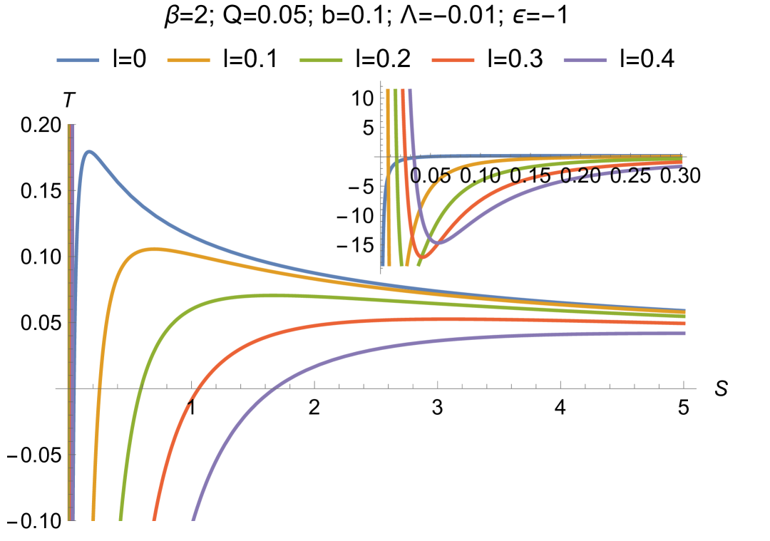
(a)

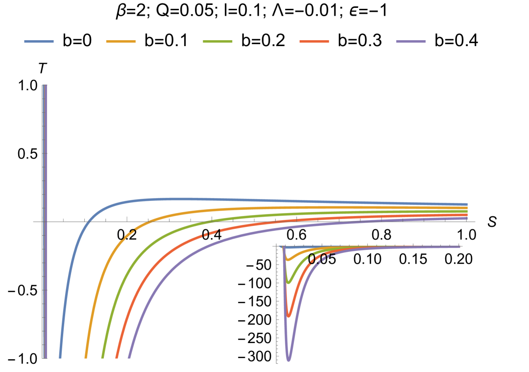
(b)

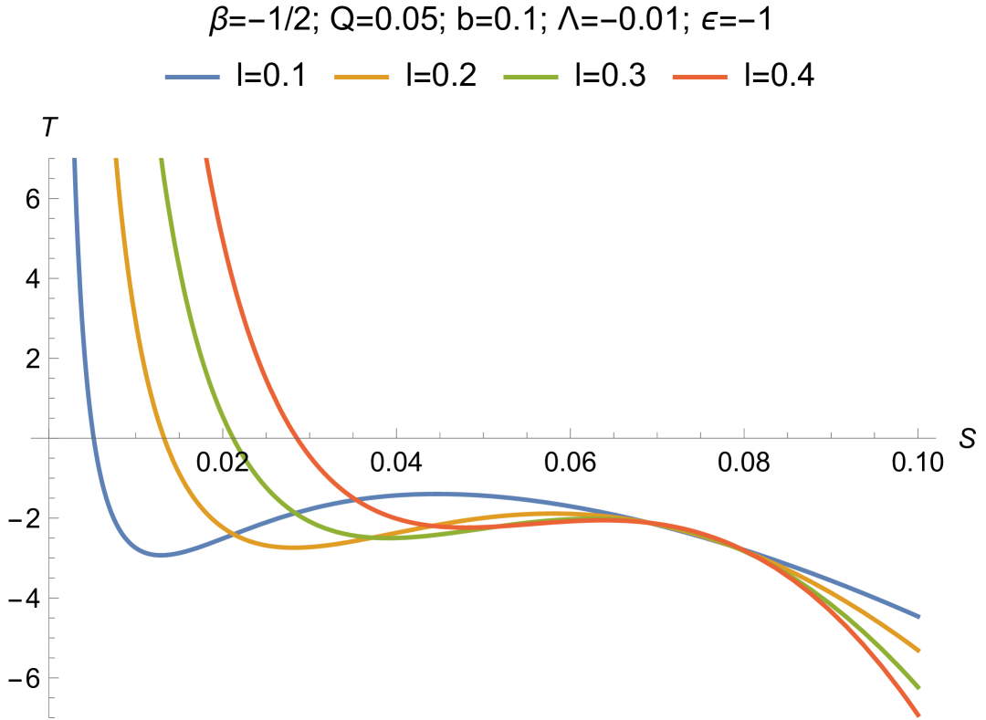
(c)

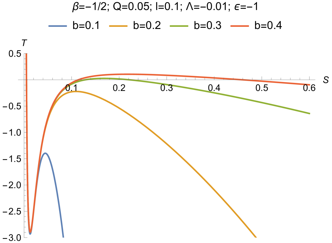
(d)

Figure 3: Black hole temperature as a function of entropy $T(S)$ for different values of $b$ and $l$.

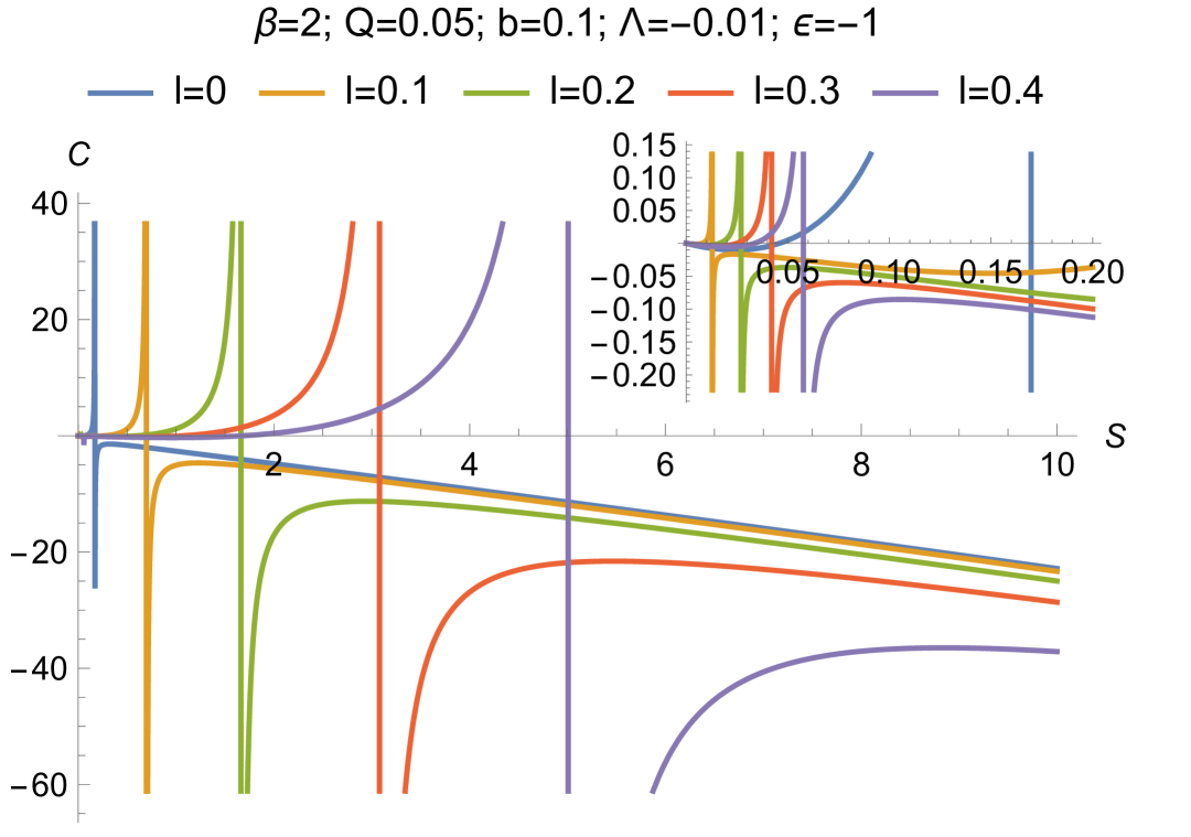
(a)

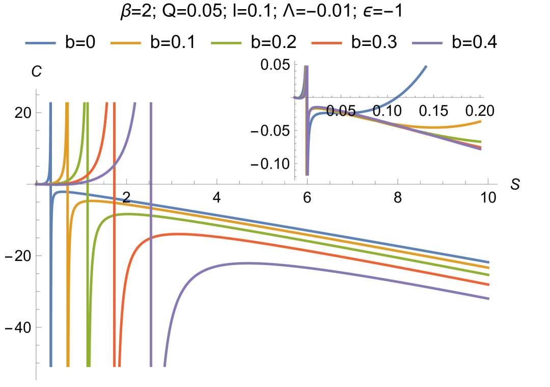
(b)

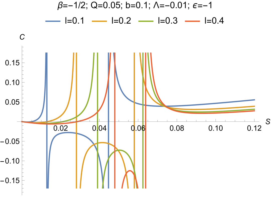
(c)

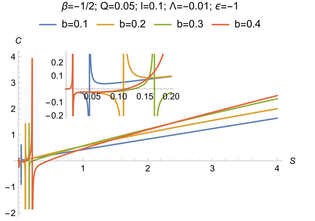
(d)

Figure 4: Heat capacity as a function of entropy $C(S)$ for different values of $b$ and $l$.

3.3 Heat capacity

In order to calculate the heat capacity of the class of solutions corresponding to the Frolov-AdS black hole with a fluid of strings, let us use the following relation:

$$C=T\frac{\partial S}{\partial T}=T\left(\frac{\partial T}{\partial S}\right)^{-1}.$$ (57)

Substituting Eq. (55) into Eq.(57), we find that the heat capacity as a function of the entropy is given by:

$$C^{(\beta=2)}= \left[2S\left(2\pi^{2}l^{2}Q^{2}+S^{2}\right)\right.$$ (58)

$$\left.[-36\pi^{9/2}bl^{4}Q^{2}\sqrt{S}\epsilon-36\pi^{4}l^{4}Q^{2}S+144\pi^{3}l^{2}Q^{2}S^{2}+108\pi^{2}l^{2}S^{3}+36\pi^{2}Q^{2}S^{3}-36\pi S^{4}\right.$$

$$\left.-9\pi^{5}b^{2}l^{4}Q^{2}\epsilon^{2}+36\pi^{7/2}bl^{2}Q^{2}S^{3/2}\epsilon+108\pi^{5/2}bl^{2}S^{5/2}\epsilon-36\pi^{3/2}bS^{7/2}\epsilon\right.$$

$$\left.+27\pi^{3}b^{2}l^{2}S^{2}\epsilon^{2}+12\pi^{7/2}b\Lambda l^{4}Q^{2}S^{3/2}\epsilon+24\pi^{3}\Lambda l^{4}Q^{2}S^{2}-72\pi\Lambda l^{2}S^{4}+36\Lambda S^{5}\right.$$

$$\left.-36\pi^{3/2}b\Lambda l^{2}S^{7/2}\epsilon-4\pi^{2}\Lambda^{2}l^{4}Q^{2}S^{3}+12\Lambda^{2}l^{2}S^{5}\right.$$

$$+08\pi^{3}b^{2}l^{2}S^{2}\epsilon^{2}\log^{2}\left(\frac{\sqrt{S}}{\sqrt{\pi}}\right)+4\pi^{7/2}bl^{2}Q^{2}S^{3/2}\epsilon\left(\Lambda l^{2}+9\right)\log\left(\frac{\sqrt{S}}{\sqrt{\pi}}\right)$$

$$\left.-18\pi^{3/2}bl^{2}\epsilon\log\left(\frac{S}{\pi}\right)\left(\pi^{3}l^{2}Q^{2}\left(\sqrt{\pi}b\epsilon+2\sqrt{S}\right)-3\pi^{3/2}bS^{2}\epsilon+2\Lambda S^{7/2}-6\pi S^{5/2}\right)\right.$$

$$\left.-9\pi^{5}b^{2}l^{4}Q^{2}\epsilon^{2}\log^{2}\left(\frac{S}{\pi}\right)]\right]/$$

$$\left[216\pi^{6}l^{6}Q^{4}S-288\pi^{5}l^{4}Q^{4}S^{2}+468\pi^{4}l^{4}Q^{2}S^{3}+72\pi^{4}l^{2}Q^{4}S^{3}-936\pi^{3}l^{2}Q^{2}S^{4}\right.$$

$$\left.-324\pi^{2}l^{2}S^{5}-108\pi^{2}Q^{2}S^{5}+144\pi^{13/2}bl^{6}Q^{4}\sqrt{S}\epsilon+288\pi^{11/2}bl^{4}Q^{4}S^{3/2}\epsilon+36\pi S^{6}\right.$$

$$\left.+648\pi^{9/2}bl^{4}Q^{2}S^{5/2}\epsilon-144\pi^{7/2}bl^{2}Q^{2}S^{7/2}\epsilon-216\pi^{5/2}bl^{2}S^{9/2}\epsilon+72\pi^{3/2}bS^{11/2}\epsilon\right.$$

$$\left.+18\pi^{7}b^{2}l^{6}Q^{4}\epsilon^{2}+207\pi^{5}b^{2}l^{4}Q^{2}S^{2}\epsilon^{2}-27\pi^{3}b^{2}l^{2}S^{4}\epsilon^{2}-48\pi^{5}\Lambda l^{6}Q^{4}S^{2}\right.$$

$$\left.-336\pi^{7/2}b\Lambda l^{4}Q^{2}S^{7/2}\epsilon-552\pi^{3}\Lambda l^{4}Q^{2}S^{4}+360\pi^{2}\Lambda l^{2}Q^{2}S^{5}+72\pi\Lambda l^{2}S^{6}+36\Lambda S^{7}\right.$$

$$\left.+216\pi^{5}b^{2}l^{4}Q^{2}S^{2}\epsilon^{2}\log\left(\frac{\sqrt{S}}{\sqrt{\pi}}\right)-8\pi^{4}\Lambda^{2}l^{6}Q^{4}S^{3}+132\pi^{2}\Lambda^{2}l^{4}Q^{2}S^{5}+12\Lambda^{2}l^{2}S^{7}\right.$$

$$\left.-108\pi^{3}b^{2}l^{2}S^{2}\epsilon^{2}\log^{2}\left(\frac{\sqrt{S}}{\sqrt{\pi}}\right)\left(2\pi^{2}l^{2}Q^{2}+5S^{2}\right)\right.$$

$$\left.+6\pi^{3/2}bl^{2}\epsilon[\right.$$

$$\left.+2\pi^{4}l^{4}Q^{4}\left(9\pi^{3/2}b\epsilon-4\Lambda S^{3/2}+24\pi\sqrt{S}\right)\right.$$

$$\left.+3\pi^{2}l^{2}Q^{2}S^{3/2}\left(7\pi^{3/2}b\sqrt{S}\epsilon-24\pi^{2}Q^{2}-12\Lambda S^{2}+16\pi S\right)\right.$$

$$\left.-3S^{7/2}\left(9\pi^{3/2}b\sqrt{S}\epsilon+36\pi^{2}Q^{2}-4\Lambda S^{2}+24\pi S\right)]\log\left(\frac{S}{\pi}\right)\right.$$

$$\left.+9\pi^{5}b^{2}l^{4}Q^{2}\epsilon^{2}\log^{2}\left(\frac{S}{\pi}\right)\left(10\pi^{2}l^{2}Q^{2}+9S^{2}\right)\right]$$

$$C^{(\beta\neq 2)}=\frac{\psi_{1}-\psi_{2}-\psi_{3}+\psi_{4}}{3\pi^{2}l^{4}Q^{2}S\left(\psi_{7}+\psi_{8}+\psi_{9}\right)+3l^{2}S^{2}\left(\psi_{10}+\psi_{11}-\psi_{12}\right)+\psi_{5}+\psi_{6}}$$ (59)

$$\psi_{1}=-\frac{36\pi(\beta-2)l^{2}Q^{2}S\left(\pi^{1/\beta}(\beta+1)\epsilon\left(\frac{b}{\sqrt{S}}\right)^{2/\beta}+\beta-2\right)}{\frac{1}{2\pi^{4}\beta S\left(2l^{2}Q^{2}+\frac{S^{2}}{\pi^{2}}\right)}}$$ (60)

$$\psi_{2}=\frac{9(\beta-2)^{2}S^{2}\left(Q^{2}-\frac{S\left(\pi^{\frac{1}{\beta}+1}\epsilon\left(\frac{b}{\sqrt{S}}\right)^{2/\beta}-\Lambda S+\pi\right)}{\pi^{2}}\right)}{\frac{1}{2\pi^{4}\beta S\left(2l^{2}Q^{2}+\frac{S^{2}}{\pi^{2}}\right)}}$$ (61)

$$\psi_{3}=\frac{3l^{2}S^{2}\left((\beta-2)\left(\frac{\Lambda S}{\pi}-3\right)-3\pi^{1/\beta}\beta\epsilon\left(\frac{b}{\sqrt{S}}\right)^{2/\beta}\right)^{2}}{\frac{1}{2\pi^{4}\beta S\left(2l^{2}Q^{2}+\frac{S^{2}}{\pi^{2}}\right)}}$$ (62)

$$\psi_{4}=\frac{\pi^{2}l^{4}\left((\beta-2)Q\left(\frac{\Lambda S}{\pi}-3\right)-3\pi^{1/\beta}\beta Q\epsilon\left(\frac{b}{\sqrt{S}}\right)^{2/\beta}\right)^{2}}{\frac{1}{2\pi^{4}\beta S\left(2l^{2}Q^{2}+\frac{S^{2}}{\pi^{2}}\right)}}$$ (63)

$$\psi_{5}=9(\beta-2)^{2}S^{4}\left(-\pi^{\frac{1}{\beta}+1}(\beta+2)S\epsilon\left(\frac{b}{\sqrt{S}}\right)^{2/\beta}+3\pi^{2}\beta Q^{2}-\beta\Lambda S^{2}-\pi\beta S\right)$$ (64)

$$\psi_{6}= 2\pi^{4}\beta l^{6}Q^{4}\left[-9\pi^{\frac{2}{\beta}+2}\beta(3\beta+4)\epsilon^{2}\left(\frac{b}{\sqrt{S}}\right)^{4/\beta}\right.$$ (65)

$$\left.-6\pi^{\frac{1}{\beta}+1}(\beta-2)\epsilon\left(\frac{b}{\sqrt{S}}\right)^{2/\beta}(\pi(9\beta+6)\right.$$

$$\left.-(\beta+2)\Lambda S)-(\beta-2)^{2}(3\pi-\Lambda S)(\Lambda S+9\pi)\right]$$

$$\psi_{7}=-3\pi^{\frac{2}{\beta}+2}\beta^{2}(3\beta-0)S\epsilon^{2}\left(\frac{b}{\sqrt{S}}\right)^{4/\beta}$$ (66)

$$\psi_{8}= 2\pi^{\frac{1}{\beta}+1}(\beta-2)\epsilon\left(\frac{b}{\sqrt{S}}\right)^{2/\beta}[3\pi\left(4\pi(\beta+1)(\beta+2)Q^{2}\right.$$ (67)

$$\left.+\beta(10-13\beta)S\right)+\beta(3\beta-0)\Lambda S^{2}]$$

$$\psi_{9}=(\beta-2)^{2}\beta\left(24\pi^{3}Q^{2}-11\Lambda^{2}S^{3}+46\pi\Lambda S^{2}-39\pi^{2}S\right)$$ (68)

$$\psi_{10}=9\pi^{\frac{2}{\beta}+2}\beta^{2}(3\beta+4)S^{2}\epsilon^{2}\left(\frac{b}{\sqrt{S}}\right)^{4/\beta}$$ (69)

$$\psi_{11}= 6\pi^{\frac{1}{\beta}+1}(\beta-2)S\epsilon\left(\frac{b}{\sqrt{S}}\right)^{2/\beta}\left[\pi^{2}(\beta(13\beta+6)+8)Q^{2}-\beta(\beta+2)\Lambda S^{2}\right.$$ (70)

$$\left.+3\pi\beta(3\beta+2)S\right]$$

$$\psi_{12}=(\beta-2)^{2}\beta\left(6\pi^{4}Q^{4}+3\pi^{2}S^{2}\left(10\Lambda Q^{2}-9\right)-78\pi^{3}Q^{2}S+\Lambda^{2}S^{4}+6\pi\Lambda S^{3}\right)$$ (71)

From Figs. 4(a)-4(d), we can conclude that there are values of $S$ for which the heat capacity is positive, just as there are values for which the heat capacity is negative. In other words, the black hole can be thermodynamically stable or unstable, and this stability is related to the values of the fluid of strings parameter. We can see that the transition point at which the heat capacity diverges changes when we vary this parameter.

In Figs. 4(a)-4(b) the transition point is shifted to the right as we increase the intensities of the parameters $l$ and $b$. For $S>6$, the Frolov-AdS spacetime with dark matter fluid ($\beta=2$) will be thermodynamically unstable, i.e., it will have a negative heat capacity. For this same system, the heat capacity increases as we decrease the parameters $l$ and $b$.

In Figs. 4(c)-4(d) the transition point is shifted to the right as we increase the intensities of the parameters $l$ and $b$. For $S>2$, the regular Frolov-AdS spacetime with fluid of strings ($\beta=-1/2$) will be thermodynamically stable, i.e. it will have a positive heat capacity. For this same system, the heat capacity increases as we decrease the $l$ parameter and increase the $b$ parameter.

4 Concluding remarks

The class of solutions we have obtained represents a generalization of the original Frolov regular black hole solution. This generalization is realized by the addition of the cosmological constant and a fluid of strings, which surrounds the black hole. It is worth calling attention to the fact that the new metrics are significantly different from the standard Frolov black hole metric , offering new physical information about the geometry and nature of the new class of black holes. Additionally, the obtained metrics give us appropriate limits, as expected, confirming the validity of the assumptions we have chosen to obtain the new class of black holes.

For all metrics obtained, an analysis was done in which concerns the behaviors of the Kretschmann scalar in order to check for the regularity or not of the metrics. Then, we concluded that the solutions are regular only for values of $-1\leq\beta<0$. Otherwise, for $\beta=1,2,3$, the metrics are not regular, as we can see from the fact that the Kretschmann scalar is divergent at the origin.

On the other hand, the analysis of the geodesics with respect to their completeness and incompleteness tells us that for $\beta=2$ and $\beta=3$, the geodesics are incomplete, as we can conclude from Fig. 1(b), and for $\beta=-1/10$. $\beta=-1/2$ and $\beta=-1$, the geodesics are complete, as can be read from Fig. 1(d). Thus, the analysis of the geodesics, for the values of $\beta$ considered, with the aim of knowing the characteristics of the spacetimes in relation to the singularity, confirms what is predicted by the results provided by the Kretschmann scalar, at least in the cases considered. This is an interesting and surprising result is that the predictions arising from the analysis of the Kretschmann scalar are confirmed by the analysis of the geodesics.

The investigations related to the black hole thermodynamics, in which concerns to mass in terms of the entropy, Hawking temperature, and heat capacity, were performed for $\beta=-1/2$ and $\beta=2$, in which cases black hole is regular or singular, respectively. In both cases, the mass parameter as a function of the entropy has positive and negative values depending on the parameters of the black hole and on the values of $\beta$.

The results related to Hawking temperature and heat capacity are significantly different from the standard ones due to the presence of the cosmological constant and of the fluid of strings, as sources. Note that they strongly depend on the value of $\beta$, as expected, and on values of the parameters characterizing the original Frolov black hole, as well as as on the parameter that codifies the presence of the fluid of strings. These new results offer interesting insights into the subject concerning the rich geometry of black holes, regular or singular, and their nature. solutions.

Acknowledgments V. B. Bezerra is partially supported by Conselho Nacional de Desenvolvimento Científico e Tecnológico - CNPq, Brazil, through the Research Project No. 307211/2020-7.

Declarations

Funding: Conselho Nacional de Desenvolvimento Científico e Tecnológico - CNPq, Brazil.

Conflict of interest/Competing interests: The authors declare that they have no conflicts of interest.

Ethics approval and consent to participate: Not applicable.

Consent for publication: The authors consent with publication.

Data availability: This study did not utilize underlying data.

Materials availability: Not applicable.

Code availability: Not applicable.

Author contribution: The authors contributed equally.

References

- \bibcommenthead
- [1] Schwarzschild, K. Uber das gravitationsfeld eines massenpunktes nach der einstein’schen theorie. Berlin. Sitzungsberichte 18 (1916).
- [2] Reissner, H. Über die eigengravitation des elektrischen feldes nach der einsteinschen theorie. Annalen der Physik 355, 106–120 (1916).
- [3] Nordström, G. Een en ander over de energie van het zwaartekrachtsveld volgens de theorie van einstein (1918).
- [4] Kerr, R. P. Gravitational field of a spinning mass as an example of algebraically special metrics. Physical review letters 11, 237 (1963).
- [5] Newman, E. T. et al. Metric of a rotating, charged mass. Journal of mathematical physics 6, 918–919 (1965).
- [6] Capozziello, S. & De Laurentis, M. Extended theories of gravity. Physics Reports 509, 167–321 (2011).
- [7] Bardeen, J. Non-singular general relativistic gravitational collapse (1968).
- [8] Dymnikova, I. Vacuum nonsingular black hole. Gen. Rel. Grav. 24, 235–242 (1992).
- [9] Mars, M., Martín-Prats, M. M. & Senovilla, J. M. Models of regular schwarzschild black holes satisfying weak energy conditions. Classical and Quantum Gravity 13, L51 (1996).
- [10] Ayon-Beato, E. & Garcia, A. Regular black hole in general relativity coupled to nonlinear electrodynamics. Physical review letters 80, 5056 (1998).
- [11] Ayon-Beato, E. & Garcıa, A. New regular black hole solution from nonlinear electrodynamics. Physics Letters B 464, 25–29 (1999).
- [12] Dymnikova, I. Spherically symmetric space–time with regular de sitter center. International Journal of Modern Physics D 12, 1015–1034 (2003).
- [13] Frolov, V. P. Notes on nonsingular models of black holes. Physical Review D 94, 104056 (2016).
- [14] Sajadi, S. & Riazi, N. Nonlinear electrodynamics and regular black holes. General Relativity and Gravitation 49, 1–21 (2017).
- [15] Hayward, S. A. Formation and evaporation of nonsingular black holes. Physical review letters 96, 031103 (2006).
- [16] Saleh, M., Thomas, B. B. & Kofane, T. C. Thermodynamics and phase transition from regular bardeen black hole surrounded by quintessence. International Journal of Theoretical Physics 57, 2640–2647 (2018).
- [17] Molina, M. & Villanueva, J. On the thermodynamics of the hayward black hole. Classical and Quantum Gravity 38, 105002 (2021).
- [18] Paul, P., Upadhyay, S., Myrzakulov, Y., Singh, D. V. & Myrzakulov, K. More exact thermodynamics of nonlinear charged ads black holes in 4d critical gravity. Nuclear Physics B 116259 (2023).
- [19] Singh, D. V. & Siwach, S. Thermodynamics and pv criticality of bardeen-ads black hole in 4d einstein-gauss-bonnet gravity. Physics Letters B 808, 135658 (2020).
- [20] Abbas, G. & Sabiullah, U. Geodesic study of regular hayward black hole. Astrophysics and Space Science 352, 769–774 (2014).
- [21] Zhou, S., Chen, J. & Wang, Y. Geodesic structure of test particle in bardeen spacetime. International Journal of Modern Physics D 21, 1250077 (2012).
- [22] Fernando, S. & Correa, J. Quasinormal modes of the bardeen black hole: Scalar perturbations. Physical Review D 86, 064039 (2012).
- [23] Flachi, A. & Lemos, J. P. Quasinormal modes of regular black holes. Physical Review D 87, 024034 (2013).
- [24] Lin, K., Li, J. & Yang, S. Quasinormal modes of hayward regular black hole. International Journal of Theoretical Physics 52, 3771–3778 (2013).
- [25] Perez-Roman, I. & Bretón, N. The region interior to the event horizon of the regular hayward black hole. General Relativity and Gravitation 50, 1–18 (2018).
- [26] Letelier, P. S. Clouds of strings in general relativity. Physical Review D 20, 1294 (1979).
- [27] Letelier, P. S. Fluids of strings in general relativity (1981).
- [28] Soleng, H. H. Dark matter and non-newtonian gravity from general relativity coupled to a fluid of strings. General Relativity and Gravitation 27, 367–378 (1995).
- [29] Riess, A. G. et al. Observational evidence from supernovae for an accelerating universe and a cosmological constant. The astronomical journal 116, 1009 (1998).
- [30] Perlmutter, S. et al. Measurements of and from 42 high-redshift supernovae. The Astrophysical Journal 517, 565 (1999).
- [31] Riess, A. G. et al. Bvri light curves for 22 type ia supernovae. The Astronomical Journal 117, 707 (1999).
- [32] Copeland, E. J., Sami, M. & Tsujikawa, S. Dynamics of dark energy. International Journal of Modern Physics D 15, 1753–1935 (2006).
- [33] Caldarelli, M. M., Cognola, G. & Klemm, D. Thermodynamics of kerr-newman-ads black holes and conformal field theories. Classical and Quantum Gravity 17, 399 (2000).
- [34] Dolan, B. P. The cosmological constant and black-hole thermodynamic potentials. Classical and Quantum Gravity 28, 125020 (2011).
- [35] Bekenstein, J. D. Black holes and entropy. Physical Review D 7, 2333 (1973).
- [36] Hawking, S. W. Black hole explosions? Nature 248, 30–31 (1974).
- [37] Hawking, S. W. Black holes and thermodynamics. Physical Review D 13, 191 (1976).
- [38] Zhang, H.-X., Chen, Y., Ma, T.-C., He, P.-Z. & Deng, J.-B. Bardeen black hole surrounded by perfect fluid dark matter. Chin. Phys. C 45, 055103 (2021).
- [39] Bronnikov, K. A. Regular magnetic black holes and monopoles from nonlinear electrodynamics. Phys. Rev. D 63, 044005 (2001).
- [40] Bronnikov, K. A. Regular magnetic black holes and monopoles from nonlinear electrodynamics. Physical Review D 63, 044005 (2001).
- [41] Nascimento, F., Bezerra, V. & Toledo, J. Some remarks on hayward black hole surrounded by a cloud of strings. Annals of Physics 460, 169548 (2024).
- [42] Vagnozzi, S. et al. Horizon-scale tests of gravity theories and fundamental physics from the event horizon telescope image of sagittarius a. Classical and Quantum Gravity 40, 165007 (2023).
- [43] Letelier, P. S. CLOUDS OF STRINGS IN GENERAL RELATIVITY. Phys. Rev. D 20, 1294–1302 (1979).
- [44] Letelier, P. Fluids of strings in general relativity. Il Nuovo Cimento B (1971-1996) 63, 519–528 (1981).
- [45] Soleng, H. H. Dark matter and nonNewtonian gravity from general relativity coupled to a fluid of strings. Gen. Rel. Grav. 27, 367–378 (1995).
- [46] Soleng, H. H. Correction to einstein’s perihelion precession formula from a traceless, anisotropic vacuum energy. General relativity and gravitation 26, 149–157 (1994).
- [47] Salgado, M. A Simple theorem to generate exact black hole solutions. Class. Quant. Grav. 20, 4551–4566 (2003).
- [48] Giambo, R. Anisotropic generalizations of de Sitter space-time. Class. Quant. Grav. 19, 4399–4404 (2002).
- [49] Dymnikova, I. Cosmological term as a source of mass. Class. Quant. Grav. 19, 725–740 (2002).
- [50] Toledo, J. M. & Bezerra, V. B. Black holes with a fluid of strings. Annals Phys. 423, 168349 (2020).
- [51] Nascimento, F., Morais, P. H., Toledo, J. & Bezerra, V. Some remarks on bardeen-ads black hole surrounded by a fluid of strings. General Relativity and Gravitation 56, 86 (2024).
- [52] Hawking, S. W. & Ellis, G. F. The large scale structure of space-time (Cambridge university press, 2023).
- [53] Wald, R. M. General relativity (University of Chicago press, 2010).
- [54] Chandrasekhar, S. The mathematical theory of black holes oxford univ. Press New York (1983).
- [55] Hawking, S. W. Particle creation by black holes. Communications in mathematical physics 43, 199–220 (1975).