Post-treatment problems: What can we say about the effect of a treatment among sub-groups who (would) respond in some way?

Abstract

Investigators are often interested in how a treatment affects an outcome for units responding to treatment in a certain way. We may wish to know the effect among units that, for example, meaningfully implemented the intervention, passed an attention check, or survived to the endpoint. Simply conditioning on the observed value of the relevant post-treatment variable introduces problematic biases. Further, assumptions such as “no unobserved confounding” (of the post-treatment mediator and the outcome) or of “no direct effect” (of treatment on outcome) required of several existing strategies are often indefensible. We propose the Treatment Reactive Average Causal Effect (TRACE), which we define as the total effect of the treatment in the group that, if treated, would realize a particular value of the relevant post-treatment variable. Given the total effect of treatment, and by reasoning about the treatment effect among the “non-reactive” group, we can identify and estimate the range of plausible values for the TRACE. We discuss this approach and its connection to existing estimands and identification strategies, then demonstrate its use with one hypothetical and two applied examples: (i) using hypothetical data to illustrate how a small number of sample statistics allow for point identification of the effect of police-perceived race on police violence during traffic stops, (ii) estimating effects of a community-policing intervention in Liberia, in locations where the project was meaningfully implemented, and (iii) studying how in-person canvassing affects support for transgender rights in the United States, among participants whose feelings towards transgender people become more positive.

1 Introduction

It is well-known that even in a randomized trial, limiting the analysis to a sub-group defined by a post-treatment variable, or otherwise conditioning on post-treatment variables, compromises treatment effect estimates, even within the sub-group in question. As cataloged by Montgomery et al., (2018), many investigators have attempted such analyses regardless. The temptation to consider such questions is understandable because, in many scenarios, the effect within such a sub-group is of great interest. For example, we may be interested in the the average effect among those who complied with a treatment, who received a well-implemented treatment, who were attentive, or who demonstrate some other mechanistic reaction that is either a pre-requisite for an effect or is of immediate interest. In some cases, these “effect among those who…” questions are of primary interest. In other cases, they arise as post hoc but important questions, particularly if no effect was detected among all study units but we recognize that implementation challenges, low compliance, inattentive participants, etc. may have led to a “watering down” of the estimated effect.

We describe a simple approach for making bounded inferences about the total effect in the sub-group that if treated, would have met some criterion of interest. We call this estimand the treatment-reactive average causal effect (TRACE). The price to be paid, however, is that we offer only partial identification. Our approach simply shows what the TRACE would be, subject to a postulated value. That postulated value is the total effect of the treatment in the sub-group that is not reactive to treatment, i.e. the group that does not show the mediating/mechanistic reaction of interest. In special cases, this can be known precisely, leading to point identification. In many other cases, investigators can reasonably argue about the sign of such an effect or its size relative to the effect in the reactive sub-group (the TRACE itself). Such assumptions can be used to tighten the credible range of TRACE values to a degree that may or may not be informative, but that accurately represents what can be claimed given the assumptions made and data observed.

In what follows, we first recount the problems associated with conditioning on post-treatment variables and the many seemingly disparate inferential settings in which this arises. These scenarios include attempts to “rescue” effects in randomized trials with implementation challenges, making use of attention screenings, examining mechanisms where mediation analysis is not feasible, and addressing selection or censorship. It also applies in cases where a treatment can influence the detectability of the mediating variable, such as screening for cancer, where we wish to know the effect among individuals who later had cancer diagnoses. Finally, it applies, and can allow point identification, in cases where an effect of the treatment on the outcome is only possible for those with a given value of the mediating variable, such as efforts to estimate the effect of police-perceived race on police violence that can occur only when police make a traffic stop. In fact, in such a case the effect can be point identified with only a few summary statistics.

We then describe our estimand and how it can be (partially) identified. We also discuss its relationship to other estimands such as: those that appear in mediation analysis (e.g. the controlled direct effect); the local average treatment effect (LATE) emerging in instrumental variable approaches; the “per protocol” effect; and the survivor average causal effect (SACE). In short, the TRACE may correspond to the SACE and LATE in special cases of interest, and we do not regard its definitional distinction from the SACE to be of great importance. However, the TRACE emerges because it is (partially) identifiable without relying on the strong and untestable assumptions common to other approaches, such as the exclusion restriction or the absence of unobserved confounding of the mediator with the outcome. While point identification is possible in special cases we describe, more often this approach simply reveals “what can and cannot be claimed about the TRACE, subject to the assumptions one is willing to make about the effect size in the group that would not experience the mediator of interest if treated.” Another feature of this approach is that it can be used even if the mechanistic variable in question was only measured in the treated group (or a random subset thereof). This provides a use for implementation data or other such variables often collected in field experiments or trials, but which are otherwise difficult to incorporate into estimation of effect sizes.

We illustrate this approach in one hypothetical and two applied examples. First, using hypothetical data, we briefly illustrate how a small number of sample statistics would allow for identification of the effect of police-perceived race on police violence during traffic stops, an area where post-treatment selection into the data has been a serious problem (Knox et al.,, 2020). We then apply the analysis to data from a randomized trial of a community policing program, in which investigators found limited active implementation of the prescribed program (Morse,, 2024). Finally, we use this approach to examine the persuasive effects of a 10-minute conversation on support for transgender attitudes among participants whose warmth towards transgender individuals increased following the intervention (Broockman and Kalla,, 2016).

2 Background

2.1 The problem

Consider the graph in Figure 1. For concreteness, let $D$ be the treatment assignment for a community policing program we wish to study. Let $M$ be some measure of whether or not the program was implemented in the community (e.g. a measure of whether patrols, community meetings, or some other intended element of the program was realized). Finally, let $Y$ be an outcome of interest. If we are interested in the effect of the program on the outcome, it would be natural to compare the outcomes in the treated group ($D=1$) with the outcomes in the control group ($D=0$). However, in doing so, we would include communities in the treated group that did not actually implement the program, and this would drive down our effect estimate. To address this, we need to somehow address the implementation issue.

A natural temptation is to look at only the group that implemented the program, effectively selecting or conditioning on $M$. However this is problematic for two reasons. First, as $M$ is post-treatment, conditioning on it might block part of the effect of $D$ on $Y$. At minimum, this requires changing the estimand of interest. A more intractable concern, however, is that we cannot typically rule out unobserved confounders of $M$ and $Y$ (shown as $U$). As $M$ is a consequence of both $D$ and $U$, it is a collider Pearl, (2009), and conditioning on it can create an association between $D$ and $U$. This can lead $D$ and $Y$ to become associated (via $D\leftarrow U\rightarrow Y$) for reasons other than the causal effect of $D$.

Figure 1: Causal structure of concern. A treatment ($D$), which is unconfounded here with the outcome of interest ($Y$) may affect $M$ in some sub-group. While some confounders of $M$ and $Y$ may be measured ($X$), we cannot rule out the presence of unobserved common causes of $M$ and $Y$ ($U$).

2.2 Examples

This arrangement appears in a wide variety of seemingly disparate inferential settings across disciplines. We discuss several classes of these settings here. These examples all share the causal structure shown in Figure 1. However, fine details of these settings can allow us to impose additional restrictions that can lead to special opportunities, such as special cases where point identification is possible as we discuss below.

Type 1. Manipulation, attention, and implementation checks.

In these cases, $M$ represents a variable that, while not fully necessary for an effect of $D$, lies on a path thought to be of central importance for $D$ to be effective. An example we expand on below would be a randomized trial in which some communities are assigned to receive a community policing program ($D$), in which the degree of implementation/realization of that program on the ground ($M$) varies widely. We may then wish that would examine how well this program worked in communities that implemented it to some satisfactory degree.

In some cases, an $M$ measuring implementation may make sense to measure only in the treated group. For example, if the program entails “community meetings with police”, then the number of such meetings is only expected to be non-zero in the treated group, and a variable like “attendance” at such meetings may be poorly defined in the control group. Investigators often collect such implementation data anyway, but then have difficulty integrating it into their quantitative analysis, not only because it is post-treatment but also because it does not exist for all units. However, such $M$ variables can still be used in the analyses proposed here, because the estimation process does not actually require data on $M$ from the control group. In fact, it requires only an estimate of the proportion of instances in which $M=1$ in the treated group.

Type 2. Mechanism of interest.

In some settings, the way a participant reacts to the treatment is thought to be important to the treatment’s effect. For example, in our application to Broockman and Kalla, (2016) below, we may wonder if the effect of a perspective-taking intervention on support for transgender non-discrimination policies depends on whether the intervention reduced animus towards transgender individuals.

These cases share the causal structure of the other types, but differ in that we are scientifically interested in the effect size both for those whose $M$ values react to $D$ and for those whose $M$ values do not. This setting also brings our approach into closer contact with questions in the mediation literature, where investigators are interested in knowing what part of an effect goes through a particular mechanism or is moderated by a particular variable. However, as we discuss below, the quantities of interest in mediation analyses do not speak to the same question. Additionally, mediation typically requires strong assumptions regarding the absence of unobserved $M-Y$ confounding, which we do not expect to be defensible in the settings we describe.

Type 3. “Necessary condition” mediators.

In this setting, $M$ is a necessary condition in order for $Y$ to possibly equal 1. An example can be found in studies of the police-perceived race of a driver ($D$) on the potential for police violence ($Y$) during a traffic stop ($M$). The chance of a traffic stop occurring is itself a function of police-perceived race. Police violence ($Y$) can be defined specifically as “police violence during a traffic stop,” which ensures that no police violence of this kind can occur if there is not a stop, i.e. $Y=0$ if $M=0$.

While this is merely an extreme case of $M$ being a mediator, we give it a separate category not only because it may seem like a different setting, but because the necessity of $M=1$ in order for $Pr(Y=1)>0$ provides additional useful information that, as elaborated below, makes point identification possible in such a case, given a handful of sample moments from the data.

Another example of this problem is found in attrition or loss-to-follow-up, including due to death. Suppose we wish to know the effect of smoking ($D$) on dementia rates ($Y$). However, dementia rates depend on age, and those who smoke may die younger than they otherwise would have. To refine this example, we can imagine that smoking is the treatment ($D$), survival to age 70 or beyond is $M$, and dementia as measured at 70 is $Y$. Note that the same problem occurs when $M$ is not “survival” but simply “present at follow-up” in long-term prospective studies where loss-to-follow-up/attrition is a major concern.

Our approach theoretically applies in these circumstances, but its practical value will depend on whether investigators are able to reason about a key quantity. Delaying technical details to below, here the assumption in question would be on “the effect of smoking on dementia at age 70, in those who would die young if they smoke.” This is difficult to imagine. Perhaps investigators could convincingly argue that those who died young due to smoking are of a more vulnerable or less hardy type, who would only be more sensitive to the effect of smoking on dementia. If that’s the case, we can argue at least that the effect in the group not surviving to 70 (had they smoked) is larger than in the survivor (under smoking) group. However, another quantity that is necessary for our identification result is not available in attrition/loss-to-follow-up settings.

Type 4. Treatment-responsive measurement of $M$.

In another setting, we may wish to know the effect of $D$ on $Y$ among those with some value of $M$, but the process or probability of measuring $M$ is itself affected by $D$. For example, suppose we wish to know the effect of cancer screening on survival, among those who had a positive result for cancer in that screening. The type of result we obtain here will depend on our ability to reason about the effect of screening on survival, in patients who if screened, would have screened negative. Reasoning about this, on it’s own or by comparison to the effect in the group who would screen positive, engages a complicated set of concerns about the effects of screening on behaviors, the false negative rate, the potential harms due to false positives, and other concerns which we take up in a separate line of research.

3 Proposal

3.1 Defining the TRACE

The target quantity of interest to us is a total effect of $D$ on $Y$ (TE), but averaged over only a certain group: those who, if treated, would have “implemented the project well” or otherwise would have a value of $M$ equal to one rather than zero. Formally, consider the “potential mediator” for unit $i$, $M_{i}(d)$. If a unit would have $M_{i}=1$ if treated, then $M_{i}(1)=1$, whereas if $M_{i}$ would be equal to zero had that unit not been treated, $M_{i}(1)=0$. Likewise, we can notate the values of $M_{i}$ under non-treatment as $M_{i}(0)$. The grouping of units according to the potential outcomes (here, for $M(1)$ and $M(0)$) is an example of the “principal stratification” approach, stemming from the seminal work of Frangakis and Rubin, (2002).

The first stratum or group of interest to us is composed of those units that, if treated, would have $M_{i}=1$, i.e. $M_{i}(1)=1$. Specifically, we are interested in the TE among those with $M(1)$, that is, $\mathbb{E}[\tau|M(1)=1]$ where $\tau$ is the (total) effect of $D$ on $Y$. We write this as $TE_{M(1)=1}$ or the TRACE. This is the quantity for which we will next provide a (partial) identification strategy.

We make three remarks. First, and analogously to working with instrumental variables, it will not be possible to literally segment the sample into those with $M_{i}(1)=1$ and those with $M_{i}(1)=0$. However, it will be possible to provide an identification result that allows us to estimate the total effect in the subgroup with $M_{i}(1)=1$ regardless. Second, we need not consider a unit’s value of $M_{i}(0)$. This contrasts with estimands—e.g. the local average treatment effect exposed by instrumental variables and the survivor average causal effect—that consider the effect in groups defined by both $M(1)$ and $M(0)$. We describe the differences between these approaches in terms of both the estimands they target and their identification requirements below.

3.2 Partial identification of the TRACE

Identification of the TRACE is difficult, owing to $M$’s status as a collider, and the existence of unobserved common cause confounders of $M$ and $Y$. In contexts where investigators believe all common causes of $M$ and $Y$ are observed (i.e., there is no $U$ on Figure 1), it would be possible to identify the effect of $D$ on $Y$ conditioning on $M$, because all the paths opened by this conditioning could be closed again. However, we consider this unrealistic in many settings, and of no interest for the problems on which we focus. For example, if $D$ is a community-driven development program, and $M$ is an indicator of whether the chosen project was actually contracted or built, then one expects many unobservable features to be common causes both of “which places manage to implement the project” and the outcomes of interest $Y$. While “social capital” or other features predictive of $M$ and $Y$ may be measurable, one cannot expect to exhaust all possible common causes. We therefore focus on the case in which $U$ cannot be ruled out.

Denote the TE in the group defined by their $M(d)$ type using $TE_{M(d)=d^{\prime}}$. For example, the TE among implementers is written $TE_{M(1)=1}$. By the law of iterated expectations,

$$TE =TE_{M(1)=1}Pr(M(1)=1)+TE_{M(1)=0}Pr(M(1)=0)$$

$$TE_{M(1)=1} =\frac{TE-TE_{M(1)=0}Pr(M(1)=0)}{Pr(M(1)=1)}$$ (1)

Given randomization of $D$, TE is identifiable, as are $Pr(M(1)=1)$ and $Pr(M(1)=0)$

$$Pr(M(1)=m) =Pr(M(1)=m\;|\;D=1)\quad\text{randomization of $D$}$$

$$=Pr(M=m\;|\;D=1)\quad\text{consistency of $M(d)$}$$

$TE$ can be estimated using its analog estimator, $\widehat{TE}=\overline{Y}_{D=1}-\overline{Y}_{D=0}$, and $\widehat{Pr}(M(1)=m)$ by its analog, $\widehat{Pr}(M=m|D=1)$. The resulting estimate for $TE_{M(1)=1}$ will be denoted $\widehat{TE}_{M(1)=1}$. Thus the only unknown on the right hand side of Expression 1 is $TE_{M(1)=0}$.

We presume that it is possible to postulate maximum and minimum values for this quantity based on area knowledge or other considerations described below. For any such range of plausible values, we identify a range of values for $TE_{M(1)=1}$. We make several remarks:

• The range of resulting $TE_{M(1)=1}$ values will be narrower when $Pr(M(1)=0)$ is smaller, i.e. when the fraction of implementers is higher.

• The entire procedure can be repeated conditioning on values of $X$, i.e. $X=c$. As both the total effect and the $Pr(M(1)=1)$ may vary by strata of $X$, the center and width of the plausible range for $TE_{M(1)=1}$ can vary by strata, potentially pointing to more and less informative strata.

• $M$ need not be well-defined in the control units. This is valuable in cases where $M$ is a type of event that is only reasonably expected or measurable in the treatment group.

Finally, a view that may be clarifying is this: in many cases, e.g. where $M$ represents implementation or delivery of the treatment, one might believe that the effect among units with $M(1)=0$ is bound to be less than the effect in the group with $M(1)=1$. In this case, investigators would know that their overall effect estimate behaves like an intent-to-treat estimate, and is diluted by those cases where implementation/delivery failed. The TRACE estimand and identification procedure simply provides a formal way of undoing such a dilution. This is quite similar to how and why instrumental variables works, except that we do not assume the absence of any direct effect of $D$ on $Y$ as required by the exclusion restriction. Instead, we parameterize the violation of such an assumption through postulating the possible effect sizes in the group with $M(1)=0$.

Types of assumptions on TRACE(0)

We emphasize that the investigator is not expected to know, nor postulate a defensible single value of, the effect of $D$ on $Y$ in the group with $M(1)=0$, i.e. the TRACE(0). In fact, the ability to remain conservatively uncertain over this quantity is central to the approach and its credibility. Nevertheless, as we illustrate, inferences can sometimes be made for the price of more defensible claims regarding the reasoned bounds on this quantity. Our experience to date suggests several most common forms of assumptions, though others are possible.

• Arguments that TRACE(0) is opposite in sign to the TRACE. In some cases, units that receive treatment but have $M=0$ can be expected to have a “negative” effect of treatment (or rather, one with opposite sign of the intended beneficial effect of treatment). For example, if a development or government program in a village promises to provide something ($D=1$) but this fails to materialize ($M=0$), it may engender greater mistrust or anger. In such cases it may be further arguable that the TRACE(0) is also smaller in absolute value than TRACE(1), though this depends on the circumstance.

• Arguments that $TRACE(0)=0$. In some cases we have reason to believe that absent the activation of $M$, there can be no effect of $D$ on $Y$. For example, in the policing application, if the police do not make a stop ($M=0$), there cannot be police violence during that stop. This leads to point identification in a way that resembles IV, with the same estimator. However, the assumption of TRACE(0)=0 differs slightly from the exclusion restriction, and the TRACE estimand yields an average effect for “compliers and always-takers” whereas IV identifies the effect over only “compliers.” We elaborate on this distinction in Section 3.4.

• Arguments that $TRACE(0)\approx 0$. In other circumstances we cannot argue that an effect is precisely impossible when $M=0$, only that we expect it to be very small for substantive reasons. For example, if the treated are enrolled in an exercise program but never participate, we expect it will have no effect, but it is possible that it has some effect by triggering other behavioral changes.

• Arguments that $abs(TRACE(0))<abs(TRACE(1))$. In many other cases we can not be certain as to the impact of $D$ on $Y$ in those with $M(1)=0$, but we can be convinced that this effect is at least less than the effect when $M(1)=1$. This means that while we do not know the TRACE, we argue that the TRACE(0) is smaller (in absolute value) than it. For example, in the community policing application below, we argue that a community randomly assigned to receive the community policing intervention but not showing evidence for its implementation or awareness of the program in the community will not have as large an effect as in those places where we do see evidence that the program occurred and was seen to occur. Fortunately, it is easy to explore the implications of such an assumption by highlighting a region of the results figure (see e.g. Figure 3) where this holds.

Finally, it is important to remember that “believing one of these assumptions” (or any other) and seeing the results is one mode of inference that may be useful. Another use case is simply to explore such assumptions and to see their implications, or to look where the TRACE produces a particular research conclusion and ask what would have to be believed about TRACE(0) to support that conclusion.

3.3 Latent DAG representation

One difficulty of using DAGs in this context is that the estimand we propose conditions on membership in a group—those units with $M(1)=1$—that cannot be conditioned on using observed variables, and thus cannot be directly represented by a conditioning procedure on the DAG. To represent our estimand (or the TRACE(0)) would thus require a modification to what appears on the DAG. The result helps to clarify why our approach works for those accustomed to graphical analysis.

Consider the value of $M(1)$ for each unit $i$ as a (latent) variable. This represents a latent “type”, or membership in either of two principal strata—that with $\{M(1)=1,M(0)=1\}$ (or “always-takers”) and that with $\{M(1)=1,M(0)=0\}$ (“compliers”). The value of $M(1)$ is a function of the unobservables, $U$, and so can be shown as a descendant of $U$ on the graph. The realized $M$ is a function of $M(1)$ and $D$. Since $M$ is also a function of $M(0)$ (when $D=0$), the $U$ variables also touch on $M$ through a path not including $M(1)$. These relationships are encoded in Figure 2. A key feature of this relationship is that there is no $D\to M(1)$ edge. If we were able to condition on $M(1)$, as a collider of $X$ and $U$, it would open the path $M\leftarrow M(1)\leftarrow X-U\rightarrow Y$. This “explains” reasons for the association of $M$ and $Y$ conditional on $M(1)$, however it does not jeopardize the identification of the $D\to Y$ effect, as conditioning on $M$ would.

Figure 2: Latent DAG representation

3.4 Connections to other approaches

Several related estimands exist that are valid in their handling of post-treatment variables, but differ in their identification and interpretation. First, we have relied here on classifying observations according to how their $M$ values would respond to $D$, so our analysis is an example of the principal stratification framework (Frangakis and Rubin,, 2002), which formalizes early work addressing treatment noncompliance with a potential outcomes framework (see e.g. Rubin,, 2000; Frangakis and Rubin,, 1999; Imbens and Rubin,, 1997; Angrist et al.,, 1996; Baker and Lindeman,, 1994). As alluded to briefly above, it can be useful to stratify observations into compliers, defiers, always-takers, and never-takers. Mapping these onto our approach, we can label those with {$M(1)=1,M(0)=0\}$ as compliers, those with $\{M(1)=1,M(0)=1\}$ as always-takers, those with $\{M(1)=0,M(0)=0\}$ as never-takers, and those with $\{M(1)=0,M(0)=1\}$ as defiers. In these terms, the TRACE is the average treatment effect for always-takers and compliers (or the “principal effect” for the stratum of always-takers and compliers), while the TRACE(0) we postulate assumed values for is the average effect over never-takers (and if present) defiers. In some settings, such as controlled medical trials, we can rule out the possibility of always takers in the sample, and so the TRACE will be the average treatment effect among compliers. This is only possible when the researcher has sufficient control to deny treatment access, or if $M$ is defined only for the treated group. For example, if we defined $D$ as a screening for cancer and $M$ as the result from that screening, it would be impossible for $M=1$ when $D=0$. Although these special cases exist, for all of the four types of settings that we describe, there exist examples for which always takers could be present.

With this in mind, Table 1 compares related estimands for different settings in which post-treatment variables are relevant. Though our estimand is unique from the rest in the group that it considers, we emphasize that the main motivation for our approach is the partial identification strategy it allows without requiring implausible assumptions such as the absence of $M-Y$ confounding or of a direct $D\to Y$ effect. In some cases, our estimand simplifies to an average effect among compliers or an average effect among always takers, for which other identification strategies exist. The novelty of our contribution lies in the relatively straightforward partial identification strategy.

Estimand	Definition	Among Whom	Identification Assumptions
LATE	$\mathbb{E}[Y_{1i}-Y_{0i}|M_{1i}>M_{0i}]$	compliers	relevance, exogeneity, exclusion restriction
CDE($m$)	$\mathbb{E}[Y(1,m)-Y(0,m)]$	all units	sequential unconfoundedness
SACE	$\mathbb{E}[Y(1)-Y(0)|M(0)=M(1)=1]$	always takers	monotonicity, explainable nonrandom survival
TRACE	$\mathbb{E}[Y(1)-Y(0)|M(1)=1]$	compliers + always takers	assumptions on $TE_{M(1)=0}$

Table 1: Comparison of different estimands for settings in which posttreatment variables are relevant

Comparison to instrumental variables.

The Local Average Treatment Effect (LATE), also called the Complier Average Causal Effect, is defined as

$$\mathbb{E}[Y_{i}(1)-Y_{i}(0)|M_{i}(0)=0,M_{i}(1)=1]$$ (2)

in this setting (Angrist et al.,, 1996; Imbens and Angrist,, 1994; Baker and Lindeman,, 1994; Angrist and Krueger,, 1991). It differs from our estimand in that it only considers the effect among compliers, while we consider the effect among compliers and always-takers. If the effect among the two subgroups is the same, then the estimands will be equivalent. This will happen in the case where there is one-way non-compliance such that there are no always-takers. Several identification strategies exist for the LATE that require additional assumptions on the causal structure of the setting (see Swanson et al.,, 2018; Angrist and Krueger,, 2001; Angrist et al.,, 1996; Imbens and Angrist,, 1994; Baker and Lindeman,, 1994). Notably, the LATE is the target estimand for instrumental variables approaches, which require that $D_{i}$ only affects the outcome through $M_{i}$. The existence of the path from $D_{i}$ to $Y_{i}$ in our setup (see Figure 1) violates this assumption.

Frangakis and Rubin, (2002) introduce the “associative effect”, which is defined as the comparison between $Y(1)$ and $Y(0)$ when $M(1)\neq M(0)$. In settings where there are no defiers, this is equivalent to the IV estimand. In settings where there are defiers, this is the effect of the treatment on the outcome among compliers and defiers – that is, it is the effect among those for whom treatment changes the value of the posttreatment variable. This allows for the treatment to affect the posttreatment variable in both possible directions, however, the aggregate quantity may not be sufficient to describe the effect of the treatment on the outcome as the effects in opposite directions among the two subgroups may cancel out.

Finally, we note a special case when TRACE(0) is reliably equal to zero. This can happen in designs where it is impossible to have an effect on $Y$ when $M=0$. For example, police-perceived race cannot affect violence at a police stop if the police stop does not occur. This arrangement closely mimics that of an IV analysis, and indeed the TRACE estimand (Equation 1) is identical to the IV estimand. This makes intuitive sense insofar as the statement “$D$ cannot influence $Y$ when $M=0$” resembles the exclusion restriction. However, there is a subtle technical distinction between the two. To assert TRACE(0)=0 is not to say “$D$ can only affect $Y$ when $M=1$”, whereas the exclusion restriction claim is that “$D$ has no affect on $Y$ but through $M$”, i.e. you can remove the $D\to Y$ edge on the DAG in Figure 1. With potential outcomes, the exclusion restriction is sometimes written as $Y(m,d)=Y(m,d^{\prime})=Y(m)$ for all $m$ and $d,d^{\prime}$ (Angrist et al.,, 1996; Imbens and Angrist,, 1994). That is: once you know the value taken by $M$, the value of $D$ has no influence on $Y$. This is clearly not the case when TRACE(0)=0: In the police stop violence case, for example, when a stop occurs ($M=1$), we imagine that the perceived race ($D$) does influence the use of violence ($Y$). Consequently, one result of our analysis is that the TRACE approach can provide an alternative to IV point identification, albeit with the same estimator. The estimand itself changes: the TRACE gives us the average effect among compliers and always-takers, while the LATE produced by IV gives the average effect among just compliers.

Comparison to survivor average causal effect.

In settings where the outcome is censored due to a post-treatment factor, the treatment reactive estimand shows up as the “survivor average causal effect” (SACE), coined as such because the relationship between treatment $D$ and outcome $Y$ is mediated by some notion of survival $S$ (Tchetgen,, 2014; Egleston et al.,, 2009; Rubin,, 2000; Robins,, 1986). The SACE is defined as follows:

$$SACE=\mathbb{E}[Y(1)-Y(0)|S(0)=1,S(1)=1]$$ (3)

where $S(d)$ is the potential value of mediator $S$ if a participant was assigned treatment status $d$. This considers only the effect among always survivors (or “always takers” in the principal stratification language, see Zhang et al.,, 2009; Rubin,, 2006; Zhang and Rubin,, 2003; Rubin,, 2000). The SACE is identified under common assumptions of SUTVA, monotonicity, and no unmeasured confounders, and an additional assumption of “explainable non-random survival”,written as

$$\mathbb{E}[Y(1)|S(0)=1,S(1)=1,X]=\mathbb{E}[Y(1)|S(0)=0,S(1)=1,X]$$ (4)

This last assumption, paired with the monotonicity assumption, essentially states that the treatment effect among “always survivors” is the same as the treatment effect among “compliers” (Egleston et al.,, 2009; Hayden et al.,, 2005). Meanwhile, our estimand describes the treatment effect among a group that includes only “always survivors” and “compliers.” When the explainable non-random survival assumption holds, the SACE is equivalent to our estimand.

In practice, this connection is only relevant for settings for which the total effect is identifiable. The survival setting deviates from settings we have thus far considered because of missingness in the outcome due to loss to follow up/death. To use our identification approach (1), we need $\overline{Y}_{1}-\overline{Y}_{0}$ to estimate the total effect, $TE$. Since we don’t have $Y$ available for all the units, this is infeasible to calculate. We could attempt to put bounds on $TE$ by first imputing 0 for all the missing values, and then imputing 1 for all the missing values, and then doing the additional reasoning about $TE_{M(1)=0}$. This will result in a fairly wide, uninformative interval for the true effect, so we don’t recommend the use of this approach for survival settings.

Outside of survival settings, this same estimand can be interpreted as the average treatment effect among always takers. Hudgens and Halloran, (2006) propose a causal estimand for evaluating vaccine efficacy which is defined as the effect of vaccine on a postinfection outcome for participants that would be infected under both treatment assignments – this is the “always infected” or “doomed” principal stratum. In setting up the problem, they make a monotonicity assumption which rules out the possibility that an individual would get infected if given the vaccine but would not get infected if not given the vaccine. Hudgens and Halloran, (2006) show that if no additional assumptions are made, the “always infected” treatment effect is not identifiable. In order to identify the effect, they consider different additional assumptions that can be made about the selection model for infection, and also consider sensitivity analyses that reason about the difference in treatment effect between the “always infected” group and the “protected” (from infection by vaccine) group. An alternative method that they consider involves reasoning about the expected outcome under control for the protected group. This is similar to our partial identification approach, but focuses on reasoning about a more specific group, the “protected” group. In the same setting, we can use our method to estimate the effect of vaccine on postinfection outcome for participants that, if vaccinated, would have been infected. We would need to reason about the same effect among participants that if vaccinated, would not have been infected.

Comparison to mediation analysis.

A variety of mediation approaches decompose the total effect into changes in the outcome that are caused directly by treatment and those that are caused indirectly through changes in the mediator (Acharya et al.,, 2016; Imai et al.,, 2014, 2010; Pearl,, 2014, 2001; Robins and Greenland,, 1992). By comparison, we focus on the estimation of this total effect for a subgroup of the population that is defined by the potential value of the mediator. This highlights a key difference: mediation approaches typically aim to isolate a path-specific effect, while our analysis isolates the total effect, for a particular subgroup.

Digging deeper, the total effect can be decomposed into the natural direct effect, which is the effect of the treatment not through the mediator, and the natural indirect effect, which is the effect of the treatment through the mediator. The natural direct effect and natural indirect effect are identified under an assumption of no intermediate confounders, in other words, an assumption that there are no consequences of the treatment that affect both the mediator and the outcome (Acharya et al.,, 2016). When intermediate confounders exist, one can instead identify and estimate the controlled direct effect – this is the effect of the treatment on the outcome, at a fixed value of the mediator. The controlled direct effect is defined as

$$CDE(m)=\mathbb{E}[Y_{i}(1,m)-Y_{i}(0,m)]$$ (5)

This differs from our estimand in that it sets a fixed value of mediator $M$, in order to isolate the path from $D$ to $Y$. Meanwhile, our estimand considers the potential value of mediator $M$ for each treatment status, and focuses on the total effect for the group where $M(1)=1$.

While one can recompose the total effect in mediation analysis from the controlled direct effect and natural indirect effects, this does not appear to be a productive path for the TRACE, for two reasons. First, the total effect is easy to identify and estimate, whereas composing it from the controlled direct and natural indirect effect requires the addition of sequential ignorability assumptions. Second, to obtain the total effect among those with $M(1)=1$ by this decomposition would further require getting the controlled direct effect and natural indirect effect also for the group with $M(1)=1$.

Intention to treat, as-treated, and per-protocol analyses.

In the RCT literature, it is common to perform an intention-to-treat (ITT) analysis, which evaluates causal effects based on the assigned treatment when not all participants adhere to treatment assignment. This estimates the effectiveness of offering a treatment, rather than the effectiveness of the treatment itself (Sheiner and Rubin,, 1995). Under nonadherence, the ITT estimate is often thought of as a conservative estimate of treatment effect, and is useful in practice due to its simplicity and the lack of assumptions. However, depending on the research question, the ITT estimate can be misleading – it is biased towards the null, which means that if we are assessing whether a treatment is harmful, the estimate will be anti-conservative. Additionally, it is possible that the ITT estimate will fail to reject the null in cases where the treatment actually did have a non-null effect (Sheiner and Rubin,, 1995; Hernán and Hernández-Díaz,, 2012).

Another common approach to estimation under nonadherence is an “as-treated” analysis, which estimates the effect of the treatment that was actually taken rather than the treatment that was assigned – in our setup, this is the effect of $M$. This effect estimate will suffer bias from confounding if the characteristics that moved a participant to treatment implementation are associated with characteristics that directly affect a participant’s outcome. In a similar vein, some researchers will instead perform a “per-protocol” analysis, which includes only the participants who adhered to treatment assignment. This is simply conditioning on the implementation variable, and poses the problems just described if the characteristics that lead to adherence are associated with characteristics that affect the outcome, sometimes referred to as post-treatment selection bias (Rosenbaum,, 1984; Robins and Greenland,, 1992).

G-estimation under a “no unmeasured $M-Y$ confounders” assumption.

For both as-treated and per-protocol analyses, if the confounders of the compliance-outcome relationship are known, they can be adjusted for using standard adjustment methods like inverse probability weighting or g-estimation. However, for both approaches, this essentially turns the RCT into an observational study, and requires the corresponding conditional ignorability assumptions (Sheiner and Rubin,, 1995; Hernán and Hernández-Díaz,, 2012; Hernán et al.,, 2013). Another similar approach would be to model the latent variable $M(1)$ for all units based on available covariates and then consider the estimated $\widehat{M(1)}$ as the moderating variable in the analysis (e.g. Vanacore et al.,, 2024). The predicted $\widehat{M(1)}$ is a noisy proxy for $M(1)$, and would likely underestimate the difference between TRACE and TRACE(0) in our setup. This type of approach would require identifying all confounders of $D$ and $M$, and may be feasible if there are many available covariates. We avoid making these kinds of ignorability assumptions, and instead focus on what can be recovered from the experimental setup through our partial identification approach.

3.5 Does this waste useful information?

The approach we propose makes very little use of the observed $M$, employing it only to get $Pr(M=1\mid D=1)$. This may seem to waste information. We show here that efforts to employ data on $M$, or observed relationships condition on the value of $M$, lead to alternative parameterizations that may be useful as one step in reasoning, but ultimately lead back to the same underlying unknowns without sharpening identification. We give several examples.

First note that we regard the TRACE(0) as unknown, but it has two components, one of which ($\mathbb{E}[Y(1)\mid M(1)=0]$ ) can be identified as $E[Y(1)\mid D=1,M=0]$ under randomization. The difficulty comes with the second component, $\mathbb{E}[Y(0)\mid M(1)=0]$. Randomization allows this to be written as $\mathbb{E}[Y(0)\mid D=1,M=0]$, but it remains unidentified. Assuming no defiers, $\mathbb{E}[Y(0)\mid D=1,M=0]$ is simply the expected non-treatment outcome among never-takers, $\mathbb{E}[Y(0)\mid\text{never-taker}]$. Thus, one has the choice of either reasoning directly about $\mathbb{E}[Y(0)\mid\text{never-taker}]$, or reasoning about the entirety of TRACE(0).

Second, one also has the choice to reason about the average non-treatment outcome among compliers, if they prefer. This is because we observe an estimate of $\mathbb{E}[Y(0)\mid D=0,M=0]$, which is composed of averages among compliers and never-takers,

$$\mathbb{E}[Y(0)\mid D=0,M=0] =\mathbb{E}[Y(0)\mid\text{ never-taker}]\frac{Pr(\text{never-taker})}{Pr(\text{never-taker})+Pr(\text{complier})}$$ (6)

$$+\mathbb{E}[Y(0)\mid\text{ complier}]\frac{Pr(\text{complier})}{Pr(\text{never-taker})+Pr(\text{complier})}$$

Having observed the left-hand side, assuming a value for either $\mathbb{E}[Y(0)\mid\text{ complier}]$ or $\mathbb{E}[Y(0)\mid\text{never-taker}]$ is enough to fix the other. That is, one could make an assumption on $\mathbb{E}[Y(0)\mid\text{ complier}]$, use the value of $\mathbb{E}[Y(0)\mid D=0,M=0]$ to back-out $\mathbb{E}[Y(0)\mid\text{never-taker}]$, and use that in turn to compute the TRACE(0) and identify the TRACE.

This leaves us with a choice among three different quantities that we could reason about in order to get a range of estimates for TRACE: TRACE(0), $\mathbb{E}[Y(0)\mid\text{never-takers}]$, and $\mathbb{E}[Y(0)\mid\text{compliers}]$. Note, however, that using the latter two quantities depends on an assumption of no defiers, which is not required if we directly reason about TRACE(0)). All three of these routes to (partial) identification are equivalent, but some may be better suited to reasoning and argumentation than others in a given context. In the cases examined here, we found it most profitable to reason directly about TRACE(0) because it refers to a substantive causal effect in a sub-group, and the nature of this sub-group can support arguments about TRACE(0), e.g. that is might have the opposite sign as the TRACE, that it is likely to be zero, negative, smaller than the effect in the other group, or something else useful for bounding.

Additionally, it may seem wasteful that this approach does not seek to learn anything from the naive comparison, $\mathbb{E}[Y|D=1,M=1]-\mathbb{E}[Y|D=0,M=1]$. However, the bias that separates this quantity from the TRACE involves the same unobservables just discussed. Consider the following breakdown of this naive comparison,

$$\mathbb{E}[Y| D=1,M=1]-\mathbb{E}[Y|D=0,M=1]$$ (7)

$$=\mathbb{E}[Y(1)|\text{complier}]Pr(\text{complier})+\mathbb{E}[Y(1)|\text{always-taker}]Pr(\text{always-taker})$$ (8)

$$\indent-\mathbb{E}[Y(0)|\text{defier}]Pr(\text{defier})-\mathbb{E}[Y(0)|\text{always-taker}]Pr(\text{always-taker})$$

$$=\mathbb{E}[Y(1)-Y(0)|\text{always-taker}]Pr(\text{always-taker})$$ (9)

$$\indent+\mathbb{E}[Y(1)|\text{complier}]Pr(\text{complier})-\mathbb{E}[Y(0)|\text{defier}]Pr(\text{defier})$$ (10)

$$=\mathbb{E}[Y(1)-Y(0)|\text{always-taker}]Pr(\text{always-taker})+\mathbb{E}[Y(1)-Y(0)|\text{complier}]Pr(\text{complier})$$ (11)

$$\indent+\mathbb{E}[Y(0)|\text{complier}]Pr(\text{complier})-\mathbb{E}[Y(0)|\text{defier}]Pr(\text{defier})$$

$$=TRACE+\mathbb{E}[Y(0)|\text{complier}]Pr(\text{complier})-\mathbb{E}[Y(0)|\text{defier}]Pr(\text{defier})$$ (12)

Thus, even if we rule out defiers, to get from the observed quantity back to the TRACE requires placing assumptions on $\mathbb{E}[Y(0)\mid\text{complier}]$, which as noted above is equivalent to reasoning about TRACE(0). While it may seem as if we are wasting information, this formalizes why the difference in means conditional on $M$ does not help in identification of the TRACE.

4 Examples

4.1 Hypothetical demonstration: Perceived race, police stops, and violence

Here we provide a brief hypothetical example to demonstrate the use of this approach in the challenging and widely discussed example of understanding the influence of perceived race on police behavior (see e.g. Knox et al., (2020)). This offers an example of the “Necessary condition mediator” (Type 3) category, in which we can argue $TRACE(0)=0$ precisely, leading to point identification—so long as the required sample moments are available.

Consider a scenario where police officers observe drivers and have a perception (accurate or not) of each driver’s race. Let $D=1$ designate that the police perceived the driver to be from a minority group. The police may then choose to stop the vehicle ($M$). During that stop, police violence may or may not occur ($Y$). Note that if a stop does not occur (so $M=0$), then there can be no violence, and thus no effect of perceived race on violence.

The TRACE(0) is taken over the group with $M(1)=0$, which could include never-takers ($\{M(1)=0,M(0)=0\}$, and defiers ($\{M(1)=0,M(0)=1\}$). Suppose, however, we that can rule out defiers, arguing that if a person is not stopped when perceived to be a minority, they would not be stopped when perceived to be non-minority. Consequently, the $M(1)=0$ group includes only never-takers, and because this group is not stopped (regardless of perceived race) there can be no police violence, and thus no effect of perceived race on violence, i.e. $TRACE(0)=0$, point identifying the TRACE.

Estimating the TRACE by this identification route requires only the sample moments required to estimate (i) the total effect, and (ii) the proportion with $M(1)=0$. The former requires knowing what fraction of encounters with perceived-minority drivers resulted in violence ($Pr(Y=1|D=1)$), and the fraction of encounters with perceived-non-minority drivers resulting in violence ($Pr(Y=1|D=0)$). This may not be directly available, but could be backed out from alternative combinations of information, such as the fraction of cases with violence involving perceived minority drivers ($Pr(D=d|Y=1)$), the overall proportion of police-perceived minority drivers ($Pr(D=1)$) in the relevant population, and the overall proportion of stops ($Pr(Y=1)$). However, we cannot estimate the second quantity, $Pr(M(1)=0)$, in cases where data on encounters is not available. This is similar to conclusions reached by other means in Knox et al., (2020), who show that the total effect can be point identified in this setting given additional data on the total number of perceived minority and the total number of white encounters (“encounters” describing any possible stop/nonstop). Using the count of total encounters among minority-perceived drivers, we could also estimate $Pr(M(1)=0)$ using $Pr(M=0|D=1)$, identifying the TRACE.

Finally, as noted in Section 3.4, the estimator this leads to is identical to that of IV, but differs in two subtle ways. First, the estimand differs in that TRACE is the effect for those with $M(1)=1$, which includes “compliers” and “always-takers”, not just compliers as for IV. Second, the exclusion restriction of IV is clearly violated here: while “there can be no effect of $D$ on $Y$ when $M=0$,” this is not the exclusion restriction in the ways usually defined. Specifically, knowing $M$ does not eliminate the need to know $D$ (i.e. $Y(M=1,d)\neq Y(M=1,d^{\prime})$) here. Or in graphical terms, the directed edge from $D$ to $Y$ cannot be removed: in the cases where a stop is made, we expect that police-perceived race ($D$) can indeed affect police violence ($Y$).

4.2 Effects of community policing on mob violence in Liberia

Our first empirical application is a field experimental study by Morse, (2024), which examines the effects of a community policing intervention in Monrovia, Liberia on mob violence, overall instances of crime, perceptions of security, and crime reporting. The intervention, which was implemented in collaboration with the Liberian National Police (LNP), involved a combination of community town hall meetings, increased foot patrols, and, as discussed in greater detail below, the formation and training of local security groups known as Community Watch Forums. Out of 93 eligible communities identified by the LNP across ten police zones in Monrovia, the country’s capital, 45 were randomly selected to receive the program over a period of 10 months. Outcomes are measured primarily using community surveys administered three months after the end of the intervention, with 20 randomly-selected adults interviewed in each community. Morse, (2024) finds that the intervention meaningfully reduced instances of mob violence, but did not reduce overall instances of crime, improve perceptions of security, or increase crime reporting.

Notably, the intervention studied in Morse, (2024) represented a “multidimensional,” coproduction-based approach to policing, aimed at both increasing reliance on the police and improving the community’s own ability to respond to security issues in a lawful manner. This approach is tailored to contexts with low existing police capacity. In such contexts, promoting cooperation with police as the sole legitimate means of addressing community security issues can be ineffective, or even backfire, if police lack the capacity to respond effectively to increasing demand for law enforcement. To avoid these potential pitfalls, the intervention incorporated training and capacity building for community-based security groups.

Community security groups existed in some form in many areas prior to the intervention; however, most were loosely organized and, importantly, had little or no connection to the LNP at the time the intervention began. A major component of the community policing intervention in question was to encourage the formation of law-abiding Community Watch Forums (CWFs), defined as “groups of concerned citizens who assist the police by sharing information about security threats; meeting regularly with the police to design proactive, collaborative strategies to combat crime; facilitating police investigations in their communities; and conducting nighttime security patrols during periods of peak crime” (page 12). Morse, (2024) attributes the success of the intervention at reducing mob violence to this component in particular.

We use the presence of a CWF (or, more precisely, community awareness of a CWF) as our primary mediator of interest $M$. Specifically, we set $M=1$ if more than 20% of community survey respondents at endline reported the existence of a Community Watch Forum that was registered with the police. Our main outcome of interest $Y$ is the average number of instances of mob violence reported by community survey respondents. Here our target estimand, the TRACE, represents the effect of the community policing intervention on reported mob violence in villages where assignment to the intervention would have resulted in the formation of a successful Community Watch Forum (hereafter “implementing types”).

Figure 3 illustrates what can be claimed about the effect among implementing types (TRACE) given any assumption about the effect among non-implementing types (TRACE(0)). The y-axis represents postulated values of TRACE(0), while the x-axis represents corresponding estimates of the TRACE. To interpret these results we consider three possible assumptions. First, suppose we assume that the effect of the community policing intervention is the same among implementing and non-implementing types (i.e. that TRACE = TRACE(0)). Under this assumption, our point estimate of the TRACE is equivalent to that of the ITT. This is represented on the plot by the intersection of the dashed lines ($\beta=-0.23$). HC2-based confidence intervals for the ITT are shown using the (blue) vertical line segments around the point estimate. Note that confidence intervals for the TRACE are larger than those for the ITT even where the two point estimates are the same. This is because the former represents an inference about a sub-group (those with $M((1)=1$, i.e. the “good implementers”).

Second, if we are willing to posit that the community policing intervention has no effect on mob violence in non-implementing type villages (i.e. that TRACE(0) = 0), we recover an effect size among implementing types of $\beta=-0.57$, more than twice the magnitude of the ITT, in the hypothesized direction (in this case, producing a negative effect on mob violence). This is equal to the LATE that would be produced by IV, though we recall that the assumption of TRACE(0)=0 is subtly different from the exclusion restriction (see Section 3.4).

Third and more practically, we would likely be unwilling to endorse either of the assumptions above in this case, especially because we use an arbitrary cutoff for the community awareness ($M$) indicator of implementation. However, we are willing to entertain the assumption that the intervention produced a larger benefit (negative effect on mob violence) among implementing types than among non-implementing types. This less-demanding assumption yields a range of valid estimates for the TRACE represented by the area above the horizontal dotted line, and thus to estimates of the TRACE that fall to the left of the vertical dotted line. To bound the result on both sides, if we posit that the effect among non-implementing types is greater than zero but smaller (in the same direction) than that among implementing types, the effect for the latter is between -0.23 and -0.57.

This analysis also illustrates that arguing for any larger benefit (negative effect) among implementing types can be sustained only if we believe the effect among non-implementing types fell in the opposite direction. That is, we would have to believe that the community policing intervention produced an increase in mob violence in these villages. Such a “backlash” effect may be plausible in this setting: if, for example, the police lack the capacity to respond to increased demand for law enforcement resulting from other aspects of the community policing intervention and there is no viable lawful community-based alternative, communities may resort to vigilante justice. Investigators and subject experts can reason about the plausibility of opposite-directional effects among non-implementing types in any given setting.

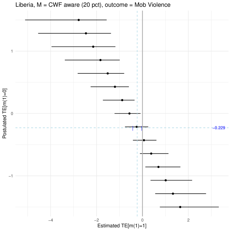
Figure 3: Estimated treatment-reactive average causal effect (TRACE) of Liberia community policing intervention on reported mob violence, among villages for which the intervention would have produced a successful Community Watch Forum (implementing types), across postulated values of the treatment effect among non-implementing types (TRACE(0)). Line segments represent 95% confidence intervals. The number on the far right represents the “naive” ITT estimate, assuming constant treatment effects across strata of $M$. All models include police zone (block) fixed effects and baseline levels of reported mob violence, averaged at the community-level, as a covariate.

This approach can also be informative in the interpretation of null findings. For example, in contrast to the encouraging findings regarding the effects on mob violence, Morse, (2024) does not find evidence that the community policing intervention reduced crime, improved perceptions of security, or increased crime reporting. Given uneven implementation, we might wonder “what would we have to believe about the effects of the intervention among non-implementing types to recover an effect in hypothesized direction among implementing types?” Figure 4 answers this question when using crime incidence as the outcome. In panel 4(a), we again use awareness of a CWF as our mediator $M$ and see that in order to obtain a significant beneficial (negative) effect among implementing types, we would have to assume a harmful effect among non-implementing types larger in magnitude than the corresponding beneficial effect among implementing types. Subject matter experts may (or may not) be equipped to convincingly reject this possibility. Panel 4(b) repeats this analysis but replacing $M$ with an alternative implementation measure capturing another major component of the community policing intervention: community town hall meetings. Here, $M=1$ if more than 20% of community survey respondents reported being aware of or having attended a community security meeting with police at endline. The results show that we cannot obtain a significant beneficial effect among implementing types even if the non-implementing group had a harmful effect almost twice as large as the beneficial effect among implementers. This increases our confidence that the failure to find an effect of the intervention on crime is not a result of uneven implementation across treated villages, at least insofar as we can consider the implementation “good enough” in those with $M=1$.

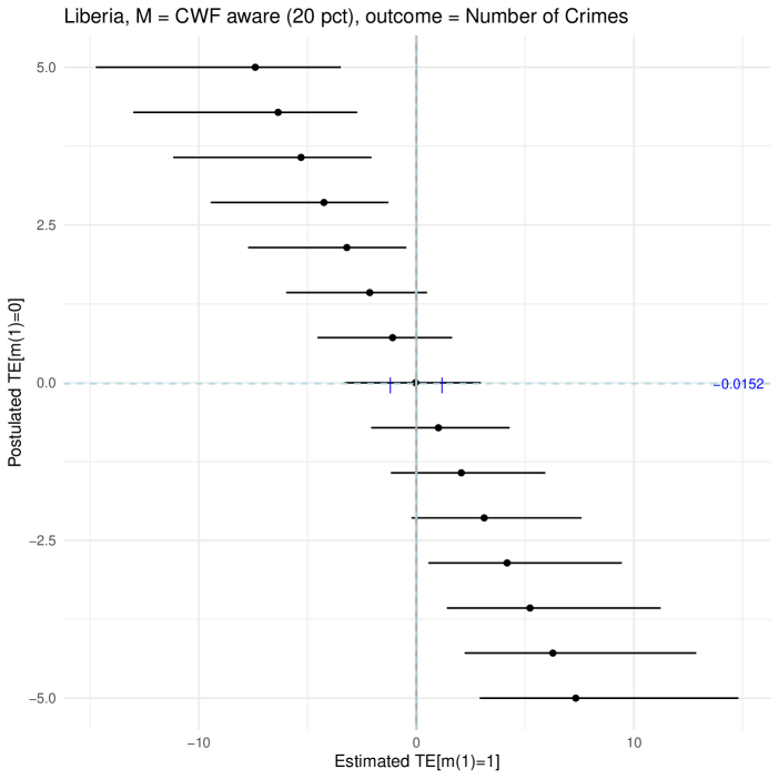
(a) Community Watch Forum (CWF) awareness as the mediator ($M=1$ if 20% of community survey respondents reported awareness of a CWF registered with police at endline).

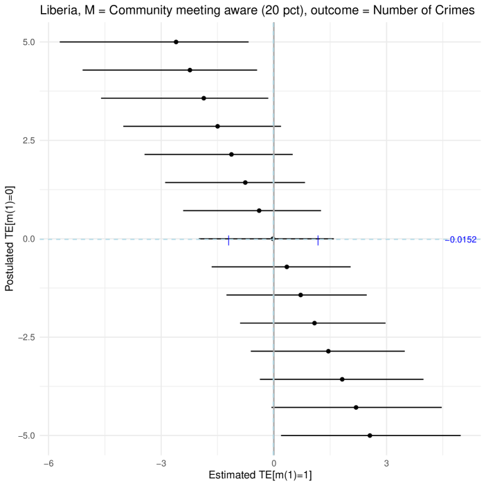
(b) Community meeting attendance or awareness as the mediator ($M=1$ if 20% of community survey respondents reported being aware of or having attended a community meeting with police at endline).

Figure 4: Estimated treatment-reactive average causal effect (TRACE) of Liberia community policing intervention on reported incidents of crime among implementing type-villages, across postulated values of the treatment effect among non-implementing-type villages (TRACE(0)), using two different implementation measures ($M$).

4.3 Empirical application 2: Effects of in-person canvassing on support for transgender rights in the United States

Our second empirical application is a field experimental study by Broockman and Kalla, (2016), which examines the effects of a door-to-door perspective taking intervention on attitudes toward transgender people and support for a transgender non-discrimination law. The intervention involved a ten-minute conversation between canvassers and voters in Miami, Florida, during which canvassers employed strategies meant to encourage “active processing,” asking voters to talk about a time when they were judged for being different, and encouraging them to see connections between their own experiences and those of transgender people. Registered Miami voters who completed a baseline survey (n = 1,825) were randomly assigned to receive either the perspective taking intervention or a placebo intervention involving a conversation about recycling. Among the 501 voters who answered the door in either condition, outcomes were measured in follow-up online surveys administered three days, six weeks, and three months after the intervention.

Building on a vast literature in psychology showing that perspective-taking can reduce prejudice against outgroups in laboratory settings, Broockman and Kalla, (2016) test whether such an intervention, outside the lab, can (i) reduce prejudice toward a stigmatized outgroup, and (ii) increase support for policies benefiting that group. They find evidence that it can: at six weeks and at three months post-intervention, treated individuals were found to be significantly more tolerant of transgender people and more supportive of an ordinance protecting transgender people from discrimination in housing employment and public accommodations.

Investigators may then wish to know what the effect of the intervention on policy attitudes would be if they could look just at individuals for whom the intervention (would have, if treated) produced a positive effect on attitudes toward transgender people. For this application, we refer to this subset as “reactive types”, noting that this shorthand is imperfect. We consider this an example of the “mechanism of interest” (type 2) question noted above. Our primary outcome $Y$ is support for the transgender non-discrimination law six weeks after treatment (wave 3), measured on a seven-point scale. Our mediator ($M$) captures the change in subjective feelings toward transgender people from baseline.

Specifically, the authors measure attitudes toward transgender people during all waves using a standard 0-100 feeling thermometer, where a higher number represents “warmer” feelings toward the group. We code $M=1$ if an individual’s thermometer score increased between baseline and wave 3, and $M=0$ otherwise. For reference, in the treatment group, thermometer scores increased between baseline and wave 3 for approximately 43% of respondents.

Figure 5 shows the results from this analysis. We illustrate interpretation with the three assumptions noted above. First, if we assume that the intervention was equally effective in increasing support for the non-discrimination law among individuals for whom it (would have) produced an improvement in subjective feelings towards transgender people and those for whom it would not have, our estimate of the TRACE is equal to the ITT (in this case, $\beta=0.27$). Second, if we instead assume no effect of the canvassing intervention on policy support among non-reactive types —those for whom it did not (or would not have) produced a positive change in attitudes toward transgender people —we recover an effect among reactive types of $\beta=0.63$. Finally, if we merely wish to assume that the effect on policy support among reactive types is greater than that among non-reactive types (but that the latter is still positively-signed), we obtain a range of estimates for the TRACE between 0.27 and 0.63. Any estimate greater than 0.63 would require an assumption of a “backlash” (negatively-signed) effect among non-reactive types.

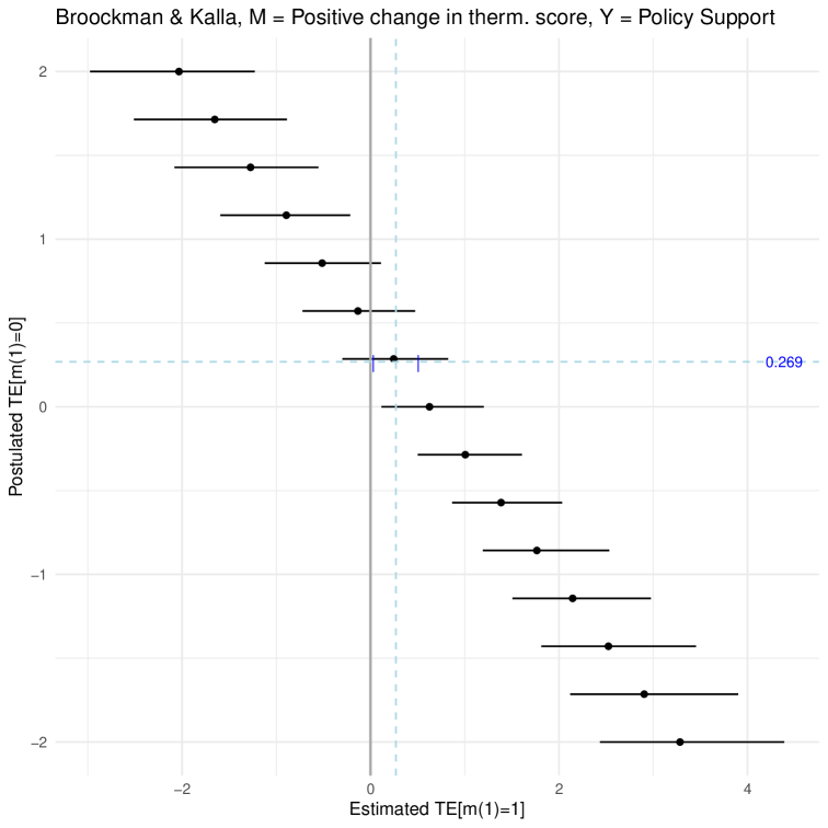
Figure 5: Estimated treatment-reactive average causal effect (TRACE) of in-person canvassing intervention on support for transgender non-discrimination law, among those for which the intervention would have led to an improvement in feelings toward transgender people from baseline (reactive types), across postulated values of the treatment effect among non-reactive types (TRACE(0)). Line segments represent 95% confidence intervals. The number on the far right represents the “naive” ITT estimate, assuming constant treatment effects across strata of $M$. All models include control variables used in Broockman and Kalla, (2016), including baseline levels of both transgender attitudes and policy support.

Our approach —and the estimand of interest —can be compared with that of Blackwell et al., (2024), who use the same empirical application. Their interest is in the controlled direct effect (CDE) of the canvassing intervention on support for the non-discrimination law, if we could hypothetically clamp (hold constant) each participant’s feeling thermometer score, leaving only the direct effect of the intervention “not through the feeling thermometer.”

Beyond requiring different assumptions (on the absence of unobserved $M-Y$ confounders) we are interested in a very different effect: the total effect of the canvassing intervention on policy support, among those whose feelings thermometer scores would have increased from baseline if given the intervention. In other words, while the CDE attempts to eliminate the effect through “warmth,” we are interested in how the intervention works both directly and through the feeling thermometer, in the sub-group that would show increased warmth due to the intervention. Nor is our estimand akin to “indirect effect” quantities found in mediation analysis, again because we are interested in both the indirect and direct effects, but for a subgroup that cannot be parsed out in mediation analysis.

5 Conclusions

In this paper, we introduce the Treatment Reactive Causal Effect (TRACE) as a novel approach for incorporating information about post-treatment variables into the estimation of causal effects. Investigators frequently face questions that require reasoning about treatment effects within subgroups defined by post-treatment characteristics, such as implementation quality, compliance, and attentiveness. Yet, as discussed by Montgomery et al., (2018) and others, directly conditioning on post-treatment variables introduces problematic biases. The TRACE provides a principled way to partially identify treatment effects for the subgroup group that, if treated, would have taken on a particular value of a relevant post-treatment variable. In comparison to existing approaches to utilizing post-treatment variables, ours does not require strong and untestable assumptions such as the exclusion restriction (as in instrumental variables approaches) or sequential ignorability (in mediation settings). Additionally, it is possible to use in cases where the relevant post-treatment variable is or can only be measured in the treatment group.

The biggest limitation is that we only offer partial identification, except in the special cases, outlined above, where point identification is possible. However, we provide a typology of reasonable assumptions that investigators may be willing to make about the effect among “non-reactive” units, which allow for bounded inferences over the TRACE. Conversely, the method can be used to ask “what would we have to assume about effects among non-reactive units to obtain a statistically significant effect among reactive units?”

While the results from our analyses may seem intuitive in many cases – it may not be surprising that assuming a smaller total effect among units that would not have implemented an intervention well implies a larger effect among those that would have – we hope readers will find value in formalizing and quantifying this assertion. Our approach may be particularly useful in the interpretation of null results from experimental studies. It is not uncommon in these cases for investigators to speculate that null results reflect uneven or inadequate implementation of the intervention. For example, in a study of coordinated community policing interventions (of which our applied example above was a part), finding no effects across contexts on citizen-police trust, cooperation with police, or crime, the authors note that “the police implemented the interventions unevenly and incompletely…” and go on to suggest that “implementation challenges common to police reforms may have contributed to these disappointing results” (Blair et al.,, 2021, 1). The approach we propose allows investigators to go beyond such statements and precisely characterize what we would have to assume in order to attribute null effects to implementation challenges.

References

- Acharya et al., (2016) Acharya, A., Blackwell, M., and Sen, M. (2016). Explaining Causal Findings Without Bias: Detecting and Assessing Direct Effects. American Political Science Review, 110(3):512–529.
- Angrist et al., (1996) Angrist, J. D., Imbens, G. W., and Rubin, D. B. (1996). Identification of Causal Effects Using Instrumental Variables. Journal of the American Statistical Association, 91(434):444–455. Publisher: ASA Website _eprint: https://www.tandfonline.com/doi/pdf/10.1080/01621459.1996.10476902.
- Angrist and Krueger, (1991) Angrist, J. D. and Krueger, A. B. (1991). Does Compulsory School Attendance Affect Schooling and Earnings? The Quarterly Journal of Economics, 106(4):979–1014. Publisher: Oxford University Press.
- Angrist and Krueger, (2001) Angrist, J. D. and Krueger, A. B. (2001). Instrumental variables and the search for identification: From supply and demand to natural experiments. Journal of Economic Perspectives, 15(4):69–85.
- Baker and Lindeman, (1994) Baker, S. G. and Lindeman, K. S. (1994). The paired availability design: A proposal for evaluating epidural analgesia during labor. Statistics in Medicine, 13(21):2269–2278. _eprint: https://onlinelibrary.wiley.com/doi/pdf/10.1002/sim.4780132108.
- Blackwell et al., (2024) Blackwell, M., Glynn, A., Hilbig, H., and Phillips, C. H. (2024). Estimating Controlled Direct Effects with Panel Data: An Application to Reducing Support for Discriminatory Policies. Working Paper.
- Blair et al., (2021) Blair, G., Weinstein, J. M., Christia, F., Arias, E., Badran, E., Blair, R. A., Cheema, A., Farooqui, A., Fetzer, T., Grossman, G., Haim, D., Hameed, Z., Hanson, R., Hasanain, A., Kronick, D., Morse, B. S., Muggah, R., Nadeem, F., Tsai, L. L., Nanes, M., Slough, T., Ravanilla, N., Shapiro, J. N., Silva, B., Souza, P. C. L., and Wilke, A. M. (2021). Community policing does not build citizen trust in police or reduce crime in the Global South. Science, 374(6571):eabd3446. Publisher: American Association for the Advancement of Science.
- Broockman and Kalla, (2016) Broockman, D. and Kalla, J. (2016). Durably reducing transphobia: A field experiment on door-to-door canvassing. Science, 352(6282):220–224. Publisher: American Association for the Advancement of Science.
- Egleston et al., (2009) Egleston, B. L., Scharfstein, D. O., and MacKenzie, E. (2009). On Estimation of the Survivor Average Causal Effect in Observational Studies when Important Confounders are Missing Due to Death. Biometrics, 65(2):497–504.
- Frangakis and Rubin, (1999) Frangakis, C. and Rubin, D. (1999). Addressing complications of intention-to-treat analysis in the combined presence of all-or-none treatment-noncompliance and subsequent missing outcomes. Biometrika, 86(2):365–379.