An interferometric study of B star multiplicity

Abstract

Context. Massive stars are extremely influential objects and multiplicity has the potential to dictate how they evolve over time by causing dynamical interactions, common-envelope evolution, mergers and more. While O-star multiplicity has been studied over a broad separation range (to the point where absolute masses of these systems have been determined and investigations into multiple system formation and interactions have been performed), studies of B star multiplicity are lacking despite the fact that they dominate the production of core-collapse supernovae and neutron stars.

Aims. Using interferometry, we aimed to investigate the multiplicity of a statistically significant sample of B stars over a range of separations ($\sim$0.5-35 au given the average distance to our sample of 412 pc).

Methods. We analyse interferometric data at high-angular resolution taken with PIONIER/VLTI for a sample of 32 B stars. Using parametric modelling of the closure phases and visibilities, we determine best-fit models to each of the systems and investigate whether each source is best represented by a single star or a higher-order system. Detection limits were calculated for companions to determine if they were significant. We then combined our findings from the interferometric data with results from a literature search to see if other companions were reported at different separation ranges.

Results. We find that, within the interferometric range, 72$\pm$8% of the B stars are resolved as multiple systems. The most common type of system is a triple system, followed by binary systems, presumably single stars and then higher-order systems. The interferometric companion fraction derived for the sample is 1.88$\pm$0.24. When accounting for the spectroscopic companions confirmed in the literature and wide companions inferred from Gaia data in addition to companions we find with interferometry, multiplicity and companion fractions of 0.88$\pm$0.06 and 2.31$\pm$0.27 respectively are obtained for our sample. The number of triple systems in particular increases significantly when accounting for spectroscopic companions, suggesting that binarity and higher-order multiplicity are integral to the evolution of B stars, as they are for O stars.

1 Introduction

Massive stars (M${}_{i}\gtrsim$ 8 M_⊙) are some of the most powerful stars in the Universe. Serving as cosmic engines, their winds, outflows and supernovae (SNe) compress and rarefact molecular clouds affecting future generations of stars. Massive stars produce the heaviest elements in the Universe and distribute these into the interstellar medium as they evolve through their end of life explosions, enriching interstellar chemistry. On galactic scales, the morphology of galactic superwinds depends on the wind activity of massive stars (Leitherer, 1994) and should a massive binary system end its lifetime as a black hole (BH) or neutron star (NS) binary merger, the subsequently released gravitational waves can be felt across galaxies (Abbott et al., 2016). However despite their importance, the formation and evolution of massive stars is still not well understood (Langer, 2012; Marchant & Bodensteiner, 2024).

One major uncertainty in the evolution of massive stars is their multiplicity. Close companions ($P_{\rm orb}$¡10yrs) in particular can have large effects on the evolution of massive stars. Mass transfer, occurring between the stars when one or both of the stars grow beyond their Roche lobe, or stellar mergers could explain apparent evolutionary inconsistencies in some single stars (de Mink et al. 2011, de Mink et al. 2013a, Schneider et al. 2019, Frost et al. 2024). A small fraction of these close binary systems result in BH mergers which create gravitational waves (Abbott et al., 2023).

In recent years the role of triples in stellar evolution has also been made evident as their evolution produces unique evolutionary channels (e.g. Toonen et al., 2016, for an overview). The existence of a third companion can affect the inner binary evolution through secular (von Zeipel, 1910; Kozai, 1962; Lidov, 1962, ZLK evolution) and quasi-secular evolution (Antonini & Perets, 2012), driving their inner binaries to close pericentre interactions, tidal interactions, migration (Mazeh & Shaham, 1979; Kiseleva et al., 1998; Eggleton & Tokovinin, 2008), mergers (Perets & Fabrycky, 2009) and/or mass-transfer. Mass loss and mass transfer in triples can also induce instabilities in such systems, change their dynamical evolution, lead to close encounters & collisions (Eggleton & Verbunt, 1986; Soker, 2004; Perets & Kratter, 2012; Shappee & Thompson, 2013; Michaely & Perets, 2014; Hamers et al., 2021; Toonen et al., 2022) and earlier interactions (Kummer et al., 2023). Therefore, the fate of a massive triple system has the potential to be significantly different to that of a massive binary system.

Most recent studies of massive stellar multiplicity thus far have focused on O-type stars which have found that the majority of massive O-type stars form in binary or higher-order multiple systems (Mason et al., 2009; Sana et al., 2006, 2012, 2013, 2014; Moe & Di Stefano, 2017; Lanthermann et al., 2023; Offner et al., 2023) and that a large fraction of these systems interact during their lifetimes (Paczyński, 1967; Podsiadlowski et al., 1992; Vanbeveren & De Loore, 1994; de Mink et al., 2013b).

While fainter, less massive and more difficult to characterise, B-type stars are responsible for their own set of unique phenomena which play important roles within the Universe. Above $\sim$25-40 M_⊙ (depending on metallicity) most massive stars directly collapse into BHs, so most SNe, both core-collapse and thermonuclear type Ia SNe, originate from B-type stars as a result of the initial mass function (IMF, Kroupa 2002). B-type stars are also responsible for the creation of most neutron stars (NS) & pulsars, and therefore are the source of long-inspiralling NS-NS mergers (e.g. GW170817, Abbott et al. 2017). The merger of two NSs also releases gravitational waves, as well as emission from gamma to radio wavelengths allowing them to be observed up to cosmological distances. Therefore, determining the B star multiplicity fraction is a keystone for understanding a wide range of astrophysical phenomena.

Abt et al. (1990) studied 109 field B stars in the Galaxy between spectral types B2 and B5 and found an observed spectroscopic binary fraction of 29%, a bias-corrected spectroscopic binary fraction 57% and a total observed binary fraction of 74% (including visual companions). Raboud (1996) determined a multiplicity fraction between 52-63% for the 56 B stars of the cluster NGC 6231. Dunstall et al. (2015) investigated the multiplicity properties of 408 B-type stars 30 Dor using the VLT-FLAMES Tarantula Survey (VFTS, Evans et al. 2011), finding a spectroscopic binary fraction of $f_{SB}$(obs) = 25$\pm$2% for most of the region, with the exception of two older clusters (Hodge 301 and SL639) whose binary fractions were 8$\pm$8% and 10$\pm$9% respectively. Using modelling and synthetic populations, they also constrained the intrinsic multiplicity properties of the less evolved dwarf and giant B-type stars in 30 Dor, allowing them to obtain a ‘present-day’ binary fraction $f_{B}$(true)=58$\pm$11%, which agreed with that found for the O-type stars in the region. Other recent work by Banyard et al. (2021) used data from VLT-FLAMES to determine a spectroscopic binary fraction of 33$\pm$5% for 80 B-type stars in the young open cluster NGC 6231, which increases to 52$\pm$8% when considering observational biases. While these spectroscopic surveys have provided a first probe of the multiplicity of these regions, the sensitivity of spectroscopic observations to multiplicity quickly drops if the period of the orbit is of order of one year and if the companions are of similar mass (Banyard et al., 2021). Beyond this period, interferometry is the technique required to search for companions (Sana et al., 2017). The $>$1 yr period domain is particularly relevant as most NS+NS mergers are expected to originate from this range (de Mink & Mandel, 2016).

In this paper we determine the multiplicity fraction for 37 B-type stars using high angular resolution data obtained with the Very Large Telescope Interferometer (VLTI, Haubois et al. 2022). We describe the observations and the model fitting used to detect companions in Section 2. We present and discuss our results in Section 3. In Section 4 we simulate artificial populations of B star multiple systems to assess how many companions may have been missed in the aforementioned work due to observational biases. Finally, we conclude in Section 5.

2 Methodology

2.1 Observations

Table 1: Information on the B stars analysed in this multiplicity study. All distances come from Gaia DR3 (Bailer-Jones et al., 2021) except for the distances which are starred and were determined by HIPPARCOS (Perryman et al., 1997). In the penultimate column we provide masses from the literature (references as footnotes. Any star that does not have information in the final column is a field star with no parent association found in the literature (as reported by the SIMBAD Astronomical Database (Wenger et al., 2000) and Cantat-Gaudin & Anders 2020).

Name RA DEC $H$mag Distance SpT Mass Comments (h m s) (^∘ ’ ”) (pc) (M_⊙) $\gamma$ Peg 00:13:14.15 $+$15:11:00.94 3.43 146${}^{+10}_{-11}$ B2 IV 8.8$\pm$0.3 $\beta$ Cep variable HD 3379 00:36:47.31 $+$15:13:54.18 6.275 279${}^{+6}_{-6}$ B2.5 IV 5.4$\pm$0.9 $\beta$ Cep variable HD 16582 02:39:28.96 $+$00:19:42.63 4.74 194${}^{+9}_{-10}$ B2 IV 8.4$\pm$0.7 $\beta$ Cep variable HD 25558 04:03:44.60 $+$05:26:08.23 5.58 222${}^{+12}_{-11}$ B5 V 4.6$\pm$0.5 HD 30836 04:51:12.36 $+$05:36:18.37 4.09 263${}^{+20}_{-18}$ B2 III 11.0$\pm$1.0 HD 32249 05:01:26.35 $-$07:10:26.27 5.30 277${}^{+10}_{-9}$ B3 IV 7.0$\pm$0.4 Orion X HD 34816 05:19:34.52 $-$13:10:36.44 4.98 299${}^{+18}_{-14}$ B0.5 V 15.0$\pm$3.5 HD 35149 05:22:50.00 $+$03:32:39.98 5.443 575${}^{+119}_{-78}$ B2 V 12.5$\pm$0.6 HD 35337 05:23:30.15 $-$13:55:38.46 5.80 370${}^{+15}_{-11}$ B2 IV 9.8$\pm$0.6 HD 37017 05:35:21.87 $-$04:29:39.04 6.88 356${}^{+8}_{-9}$ B1.5 V 6.4$\pm$0.5 HD 51480 06:57:09.38 $-$10:49:28.06 5.12 1106${}^{+31}_{-25}$ Besh 6.4$\pm$0.5 Be star HD 66765 08:02:55.72 $-$48:19:29.95 7.01 372${}^{+12}_{-9}$ B1.5 V 6.6$\pm$1.0 HD 67621 08:06:41.61 $-$48:29:50.59 6.86 355${}^{+7}_{-6}$ B2 IV 5.5$\pm$0.5 Vel OB 2 - cluster HD 105382 12:08:05.23 $-$50:39:40.58 4.95 109${}^{+2}_{-2}$ B4 III 5.7$\pm$0.4 Lower Cen Crux/Sco OB 2-4, Be star HD 109026 12:32:28.01 $-$72:07:58.76 4.25 117${}^{+4}_{-4}$ B3 V 5.0$\pm$0.5 Pulsating variable HD 116658 13:25:11.58 $-$11:09:40.75 1.54 ^∗77${}^{+4}_{-3}$ B1 V 11.4$\pm$1.2 $\beta$ Cep variable HD 121743 13:58:16.27 $-$42:06:02.71 4.46 140${}^{+7}_{-6}$ B2 IV 8.5$\pm$0.3 II Sco/Upper Cen Lupus, Variable HD 132058 14:58:31.93 $-$43:08:02.27 3.25 ^∗117${}^{+3}_{-2}$ B2 III 8.8$\pm$0.2 HD 133518 15:06:55.97 $-$52:01:47.24 6.666 602${}^{+23}_{-30}$ B2 VpHe 6.3$\pm$0.5 HD 140008 15:42:41.02 $-$34:42:37.46 5.11 128${}^{+3}_{-3}$ B5 V 4.5$\pm$0.5 Upper Cen Lupus/ Sco OB 2-3 HD 147932 16:25:35.08 $-$23:24:18.79 5.92 122${}^{+1}_{-1}$ B5 V 5.0$\pm$0.5 Ass Sco OB 2-2/Upper Sco/Ophiuchus, Rotationally variable HD 161701 17:47:36.78 $-$14:43:32.97 5.88 167${}^{+1}_{-2}$ B9III pHgMn 3.96$\pm$0.14 HD 178175 19:08:16.70 $-$19:17:25.05 5.39 414${}^{+24}_{-22}$ B2 Ve 8.8$\pm$0.6 Be star HD 189103 19:59:44.18 $-$35:16:34.70 4.79 208${}^{+14}_{-13}$ B3 IV 6.6$\pm$0.1 HD 191263 20:08:38.28 $+$10:43:33.11 6.656 441${}^{+11}_{-13}$ B3 V 6.0$\pm$0.5 HD 193933 20:23:26.26 $-$14:15:23.17 7.068 440${}^{+10}_{-10}$ B5 IV 5.6$\pm$0.5 HD 205637 21:37:04.83 $-$19:27:57.65 4.91 269${}^{+14}_{-13}$ B3 V 8.6$\pm$0.5 Be star HD 212076 22:21:31.08 $+$12:12:18.66 4.803 ^∗498${}^{+81}_{-61}$ B2 Ve 12.5$\pm$0.7 Be star HD 212571 22:25:16.62 $+$01:22:38.63 5.37 330${}^{+14}_{-11}$ B1 III-IVe 10.7$\pm$0.7 Be star HD 224990 00:02:19.93 $-$29:43:13.60 5.41 207${}^{+6}_{-5}$ B5 V 5.5$\pm$0.5 Cl Blanco 1 (open galactic cluster) MCW 1019 22:00:07.93 $+$06:43:02.81 6.212 453${}^{+27}_{-21}$ B3 III 6.9$\pm$0.7 $\tau$ Lib 15:38:39.37 $-$29:46:39.90 4.05 112${}^{3}_{-2}$ B2.5 V 7.25$\pm$0.49 II Sco/Upper Cen Lupus

The data for our sample were taken with the PIONIER instrument (Le Bouquin et al., 2011) which combines the beams of four telescopes at the VLTI in the H-band (1.66 $\mu$m, $\lambda$/$\Delta\lambda\sim$5, bandwidth$\sim$0.3 $\mu$m). The PIONIER data were reduced using the automated PIONIER pipeline (PNDRS, developed by Le Bouquin et al. 2011). PIONIER combines the signal from either the four 8.2 m Unit Telescopes (UTs) or the four 1.8 m Auxiliary Telescopes (ATs). Visibilities and closure phases are therefore obtained over six baselines and three closure phase triangles for both instruments. The observations of our sample were taken with the 1.8 m Auxiliary Telescopes (ATs). Each science observation was bracketed by a calibration observation which allows the visibilities and closure phases to be calibrated. The projected baseline lengths, $B$, range from $\sim$10-200 m with the ATs, corresponding to a resolution of $\sim$1-20 mas. PIONIER uses single-mode fibres, therefore the field of view corresponds to the point spread function (PSF) of the telescope delivered at the fibre injection point, which is $\sim$190 mas for the ATs in the H band. Most of the observations were taken over a sequence of nights in visitor mode as part of ESO programme 093.C-0503(A) (PI: H. Sana), with additional epochs of data taken from ESO programme 112.2624 (PI: L. Mahy).

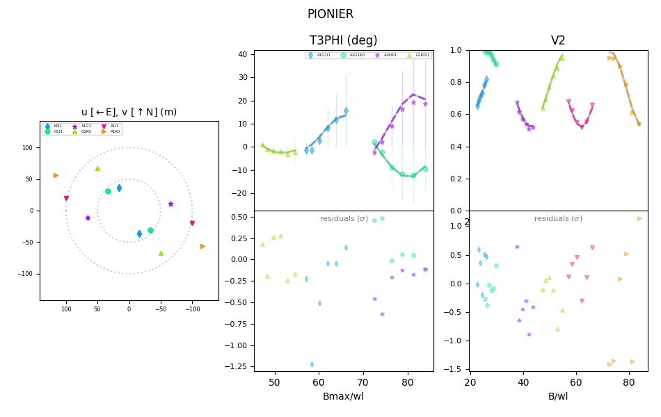
Figure 1: An example of a typical fit to the data of one of our sources HD 3379. On the left, the $u-v$ coverage from the observations with PIONIER can be seen. The different colours correspond to the telescope pair with which that particular data was acquired at the VLTI. In the middle, the closure phase (T3PHI) fit and residuals are shown in terms of the spatial frequency (B_avg/$\lambda$, written as Bavg/wl on the axes). On the right, the fit to the squared visibilities (V2) and the associated residuals are shown, again in terms of spatial frequency. Across the two fits, the data are represented as points whilst the fit is a continuous line.

Figure 2: Left: model image created based on the best-fit model to the data shown in Figure 1, showing the primary (1) and secondary (2) stars needed in the model to reproduce the interferometric observables. The colour bar displays the arbitrary flux of the star. Right: spectral energy distribution (SED) displaying the flux ratios of the stars in the model.

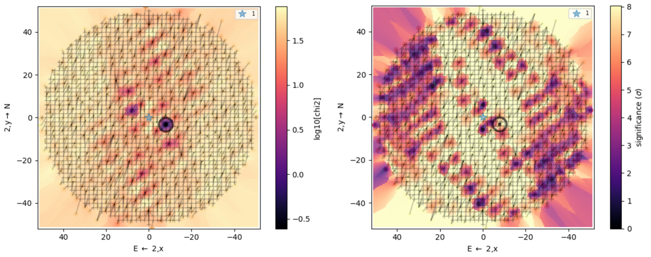
Figure 3: Plots illustrating an example of the grid fit, in this case for HD 3379. On the left, we see the grid of potential companion positions that was searched in terms of goodness of fit, as quantified by the $\chi^{2}$. The primary star, which is fixed at position (0,0) during the fit, is shown by a blue star. The black circle shows the (x,y) position of the companion in the best-fitting model. On the right, the grid is shown in terms of companion significance, allowing us to determine if a companion determined by the best-fitting model is significant in terms of its flux.

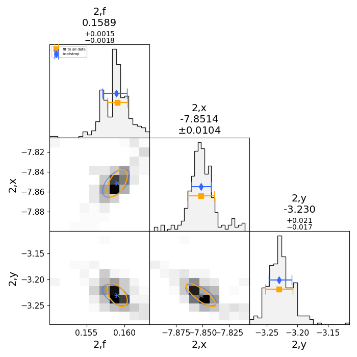
Figure 4: Bootstrapping plot showing the error determination for the dataset fit in Figure 1.

2.2 Sample Selection

The initial sample we analysed is comprised of 37 B-type objects. Much of the data of the stars was obtained during visitor mode observations in 2014 and 2015. As a result, three main selection criteria for the sample existed; their likelihood to be NS progenitors, their visibility in the sky (which is dependent on the time of the observations) and the observing capabilities of PIONIER. In order to be successfully observed with the instrument, given the typical seeing conditions at Paranal Observatory of 0.6-0.8”, objects must have, on average, a $H$-band magnitude $\lessapprox$8 mag. In comparison to other multiplicity studies such as SMaSH+ (Sana et al., 2014) which focused on O-stars, our sample is limited to closer stars as B-type stars are intrinsically fainter. The majority of the sample are within 500 pc with distances determined from Gaia eDR3 (Bailer-Jones et al., 2021) or HIPPARCOS (Perryman et al., 1997). Most of this sample were dwarf stars, followed by sub-giants, giants and supergiants. However, we do not include the supergiant stars in this work, as B supergiants are likely evolved from O-type stars, and thus they do not contribute to our aim to study B star multiplicity. Removing the supergiants leaves us with a final sample size of 32 stars, which are listed in Table 1. We searched the literature for dedicated studies providing mass estimates. When we could not find any but found papers listing atmospheric parameters (allowing us to place the star in an Hertzprung-Russell diagram), we used the bonnsai tool (Schneider et al., 2014) to obtain an evolutionary mass through a comparison with the galactic evolutionary tracks of Brott et al. (2011). When none were available, we used mass estimate from Kervella et al. (2019). Masses $M$ are a useful input for Sect 4 where we evaluate the detection capabilities of our survey. Very precise masses are however not needed as spectroscopic and interferometric detection thresholds only depends on $M$ following $M^{1/3}$.

2.3 Model fitting

Parametric fitting is performed on the PIONIER data using the Python3 module PMOIRED (Mérand, 2022), which allows the display and modelling of interferometric data stored in the OIFITS format.

We use the grid-search capabilities of PMOIRED to search for companions, which is based on a previous tool, CANDID (Gallenne et al., 2015). In the case of searching for a first companion, the model was composed of a primary star and a companion, represented by uniform disks. The position of the primary star was always fixed at (0,0) and the flux of the primary star was fixed at 1, so that the flux of any companions were presented in relation to the flux of the primary. The observables fit were the squared visibilities (V2) and the closure phases (T3PHI). An exploration dictionary was defined which the grid fit iteratively searches over various $x$,$y$ positions. The grid search then fits the observed data at each point in this defined grid. The number of positions probed depends on the amount and quality of the data, and having a grid that is too fine or coarse can result in an unreliable solution. The quality of each of the fits across the grid is assessed using the $\chi^{2}_{red}$ and this is used to find the final/best fit of the grid. Additionally, priors were used to make sure that the flux of a found companion remained greater than 0. At the start of fitting all sources, we assumed that the companion is unresolved, so its angular diameter is fixed to 0.2mas. If models with unresolved stars were not sufficient, models were run where the diameter of the stars could also be free parameters. Following the grid fitting, we used bootstrapping to determine the errors on our derived measurements of the sources and to check the final values. In the bootstrapping procedure, data is drawn randomly to create new datasets and the final parameters and uncertainties are estimated as the average and standard deviation of all the fits which were performed.

Tests were run on all companions to test the significance of any detected companions. As the grid search already computes the $\chi^{2}_{red}$, the $\chi^{2}_{red}$ statistics and the number of degrees of freedom can be used to define the significance of each of the fits across the grid in terms of $\sigma$. We note that the code saturates numerically for high significance values, so to stay reliably within numerical accuracy the maximum significance quoted is 8-$\sigma$ which corresponds to a 10^-15 chance of false detection. If a binary companion was found not to be significant, we instead ran single star fits, where the parameter fit is simply the diameter of the star.

We also attempted fits of higher order multiple system during our analysis. We did this using the following methodology. First, a binary model was fit. Then, if the fit to the data still appeared poor, we ran a grid fit for the next companion. The position of the secondary companion already found would be fixed during this search, and the grid would iterate on the position of the potential tertiary companion and so on and so forth. Running a grid fit first allowed us to determine the level of total fits and the number of steps across a grid fit that would be appropriate. We then used these values to run a search to determine a detection limit, following the methods of Absil et al. (2011). Additionally, the significance of flux determined at the best-fitting positions for any found companions was tested, and we considered any companion with a flux within a 3-$\sigma$ flux distribution to be significant. If the flux of the determined companion was found to be significant and above the detection limit across all epochs of data we analysed, we concluded that the system was a higher-order multiple system. A couple of key exceptions applied. If an additional companion’s (e.g. tertiary’s) position overlapped with the position of the previous found binary, we did not consider this a valid higher-order multiple. If there was degeneracy in the first binary grid fit due to sparse u-v coverage and an additional companion was essentially a mirror of a previously found companion because of this, we did not consider this a valid higher-order multiple either. Finally, if the position of the companion was inconsistent across different epochs of data (where they existed) without a significant time difference between epochs (of the order of weeks to months), we did not consider this a valid higher-order multiple. The latter case only occurred for a couple of sources (an insignificant fraction of the sample). In the case of variable flux across epochs, this was accepted in the case of systems that were known variables, but not accepted in systems where variability had not been previously reported in the literature. For our sample, interferometric triples were found that fulfilled all these criteria, but no higher-order multiple systems such as quadruples.

Table 2: Details on the multiplicity of the systems derived from the best-fitting datasets. $F$ represents the flux ratio of the components with relation to the brightest components (whose flux is set to 1 as a reference point). The subscript number represents whether the companion is a binary (2), tertiary (3) etc. The best fitting datasets are presented, quantified by the reduced chi-square $\chi^{2}_{red}$. Systems marked with asterisks are discussed in Section 3.4. We include the distribution of 3-$\sigma$ detections in terms of flux ratio in the last column.

Name Type $\chi^{2}_{red}$ $F_{2}$ $\rho_{2}$ $F_{3}$ $\rho_{3}$ 3-$\sigma$ detection (mas) (mas) distribution HD 16582 Single 0.34 0.002 - 0.011 HD 51480* 1.72 0.22 - 1.02 HD 66765 0.54 0.016 - 0.098 HD 67621 0.34 0.005 - 0.021 HD 121743 0.31 0.005 - 0.041 HD 189103 0.56 0.004 - 0.023 HD 205637 1.21 0.005 - 0.073 HD 212571 0.37 0.008 - 0.025 MCW 1019 2.59 0.047 - 0.120 $\gamma$ Peg Binary 0.11 0.036${}^{+0.001}_{-0.004}$ 85.6$\pm$0.1 0.026 - 0.330 HD 3379 0.25 0.159${}^{+0.002}_{-0.002}$ 8.49$\pm$0.03 0.005 - 0.018 HD 25558 3.15 0.793${}^{+0.05}_{-0.03}$ 92.56$\pm$0.20 0.020 - 0.088 HD 30836 0.99 0.060${}^{+0.04}_{-0.02}$ 3.39$\pm$0.43 0.010 - 0.073 HD 32249 16.22 0.616$\pm$0.01 31.49$\pm$0.04 0.071 - 0.278 HD 34816 0.77 0.049${}^{+0.004}_{-0.003}$ 62.7$\pm$0.1 0.026 - 0.084 HD 35337 0.37 0.038${}^{+0.002}_{-0.002}$ 9.84$\pm$0.16 0.037 - 0.127 HD 35149 0.92 0.537$\pm$0.008 23.34$\pm$0.09 0.427 - 1.23 HD 37017 0.26 0.16${}^{+0.02}_{-0.01}$ 1.00$\pm$0.05 0.157 - 0.756 HD 105382 3.79 0.066${}^{+0.003}_{-0.005}$ 41.9$\pm$0.5 0.102 - 0.397 HD 109026 0.15 0.376${}^{+0.002}_{-0.001}$ 12.94$\pm$0.02 0.003 - 0.014 HD 133518 0.45 0.085${}^{+0.377}_{-0.067}$ 0.61$\pm$3.74 0.019 - 0.057 HD 140008 0.22 0.952${}^{+0.002}_{-0.003}$ 1.130$\pm$0.006 0.398 - 0.938 HD 178175 0.32 0.0245${}^{+0.0006}_{-0.001}$ 4.76$\pm$0.06 0.006 - 0.017 HD 191263 0.48 0.39${}^{+0.14}_{-0.01}$ 1.67$\pm$0.09 0.014 - 0.073 HD 212076 0.46 0.28${}^{+0.4}_{-0.3}$ 0.42$\pm$2.60 0.013 - 0.092 HD 224990 0.62 0.270${}^{+0.002}_{-0.003}$ 33.4$\pm$0.1 0.015 - 0.054 $\tau$ Lib 2.11 0.11${}^{+0.02}_{-0.01}$ 7.62$\pm$0.2 0.066 - 0.693 HD 116658 Triple 2.15 0.078${}^{+0.03}_{-0.01}$ 0.993$\pm$0.3 0.2059${}^{+0.010}_{-0.006}$ 1.687$\pm$0.2 0.047 - 0.178 HD 132058 0.21 0.0213$\pm$0.002 6.5624$\pm$0.1 0.012${}^{+0.002}_{-0.002}$ 73.7$\pm$0.2 0.009 - 0.050 HD 147932 0.55 0.1122${}^{+0.004}_{-0.003}$ 6.70$\pm$0.1 0.028$\pm$0.003 83.0$\pm$0.3 0.015 - 0.051 HD 161701 0.11 0.219$\pm$0.002 1.15$\pm$0.1 0.052$\pm$0.003 2.89$\pm$0.06 0.016 - 0.090 HD 193933 0.11 0.624$\pm$0.1 6.17$\pm$0.02 0.021${}^{+0.003}_{-0.005}$ 16.5$\pm$0.6 0.007 - 0.037

3 Results & Discussion

Following the fitting of the PIONIER data, we detect interferometric companions around 23 of the 32 B stars in our sample. A variety of multiple systems are determined through interferometry and presented in Figure 5. Binaries are the most common system detected with interferometry (19), followed by single stars (13) and then triple systems (5). The final fits obtained to the PIONIER data of our sample is presented in Table 2. We note which sources are single, and in the case of multiple systems, the fluxes and separations of the sources with respect to the central star. For sources where multiple datasets are available, the results of the best-fitting epoch are shown. There is no discrepancy between the type of multiple system derived for a source between its datasets at different epochs. In this paper we do not discuss the multi-epoch data in detail - this is relegated to future work.

We calculate the multiplicity fraction ($f_{\mathrm{m}}$), or the ratio of the number of multiple systems ($N_{\mathrm{m}}$) to the sample size ($N$), of our sample following the definitions of Sana et al. (2014). Within our interferometric sample, $f_{\mathrm{m}}(N_{\mathrm{m}}/N)$=0.72$\pm$0.08. The statistical error on $f_{m}$ is calculated using binomial statistics ($\sigma_{f_{\mathrm{m}}}$($f_{\mathrm{m}}$, $N$) = $\sqrt{f_{\mathrm{m}}(1-f_{\mathrm{m}})/N}$, Sana et al. 2014). Similarly the interferometric companion fraction (the average number of companions per central object or the ratio of the total companions ($N_{\mathrm{c}}$) to $N$) is $f_{\mathrm{c}}(N_{\mathrm{c}}/N)$=1.88$\pm$0.24. The uncertainty on $f_{\mathrm{c}}$ is calculated following Poisson statistics and computed as $\sigma_{f_{\mathrm{c}}}$ = $\sqrt{N_{\mathrm{c}}}$/$N$ (Sana et al., 2014).

Figure 6 shows the variety of positions and fluxes of the companions to the systems. For the binaries, the average companion is 27% the brightness of the primary star and the average separation is 23 mas with a wide range of separations ($\sim$1-90 mas).

One concern when detecting new companions can be with regards to chance alignment, especially in clusters. The likelihood of chance alignment causing a false companion detection has been studied in detail for other multiplicity surveys. Sana et al. (2014) determined, for their sample of 279 stars, a probability of spurious detection due to chance alignment. This method has also proven robust in other multiplicity works such as Reggiani et al. (2022). In Sana et al. (2014), they conservatively assume that all their PIONIER (and NACO) observations are sensitive to separations up 0.2” and found that the probability of spurious detection is always smaller than 0.001%, making their interferometric detections essentially free of spurious detections. Given we use the same datasets, it is therefore likely that our detections too are free from contamination by chance alignment.

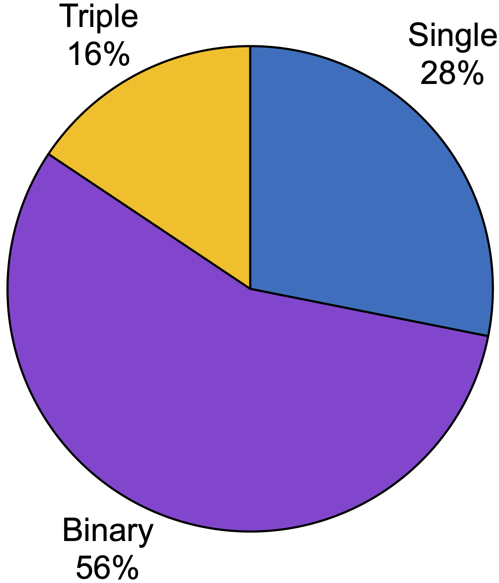
Figure 5: The percentage of the different kinds of multiple systems detected with interferometry for our B star sample.

Figure 6: Distribution of companions compared to their flux. Companions belonging to cluster sources are labelled with green arrows, the remaining sources are field stars. The symbols illustrate which companion the point represents: binary companions are represented by a circle and tertiary companions by a triangle.

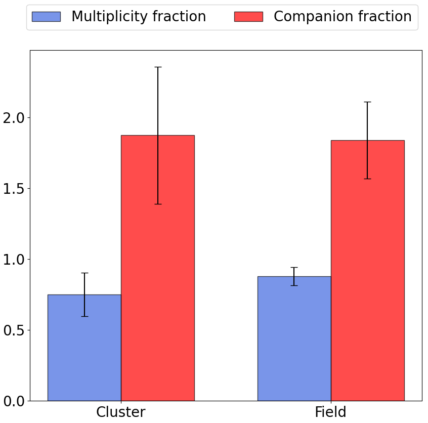
Figure 7: Bar chart displaying the change in interferometric multiplicity and companion fraction for the sources in clusters against those in the open field.

3.1 Trends

After determining the multiplicity properties of our sample, we sought to investigate whether the characteristics of the stars or their environments had any tangible affect on the number and nature of the companions. Our findings are discussed in the following sub-sections.

3.1.1 Trends with source location: cluster vs. field

First we investigate the impact of location on the type of multiple system derived. Out of the sample of 32 stars, only 8 were found to be part of a cluster or stellar association, meaning that we are dealing with small number statistics. Still, for completeness, we note that all but two of the cluster systems are multiples corresponding to $f_{m}$=0.75$\pm$0.15, with a companion fraction of 1.88$\pm$0.5. The multiplicity fraction for the cluster sources us larger than the field sources, where $f_{m}$=0.71$\pm$0.09. All these fractions are shown in Figure 7. This is consistent with the hypothesis that a cluster environment could give rise to disruption of wide systems through dynamical encounters, leading to more single stars. That being said, the field sources have a companion fraction of $f_{c}$=1.88$\pm$0.28, which is equivalent to the cluster sources (within errors). Thus we conclude that a sample including more cluster sources is required for real conclusions to be made as to the differences or lack there of between the multiplicity and companions of B stars in cluster vs. field environments.

Stellar evolution and age could also affect the multiplicity. Some of our older systems might have had more massive companions that already evolved to explode as supernovae that either disrupted the system or led to a compact companion beyond our detection limits. Therefore, there is some potential bias for older systems to be seen having lower multiplicity, which would also propagate to dependencies on both stellar type (see next section) and the environment. Since field stars might be, on average, older than cluster stars, this could then also decrease the multiplicity fraction among field stars as seen in our sample. Much work has been done in the literature to determine the ages of stellar clusters, and as a result we can speculate on the ages of our cluster sources. The majority of our cluster sources come from the Sco association. This cluster has been postulated to be between 4 and 8 million years old (Banyard et al. 2021 and references within). Within our Sco sources we see a mix of single, binary and triple systems. The remaining systems are in the Orion X association (HD 32249), the open galactic cluster Blanco 1 (HD 224990) and the Vel OB 2 cluster (HD 67621). The first two are both interferometric binaries whilst the latter appears to be a single star. Blanco 1 is estimated to be 100-150Myr (Moraux et al., 2007) in age, much older than the Sco association. Given our small sample and the lack of trends seen, we again do not make any conclusions regarding the multiplicity we detect with age.

Figure 8: The interferometric multiplicity and companion fractions for the B stars based on their luminosity class.

Figure 9: The interferometric multiplicity and companion fractions for the B stars based on their spectral sub-type.

3.1.2 Trends with luminosity class

The first stellar characteristic we investigate is the luminosity class, or in other words the evolutionary stage of the source. We only considered sources for which the luminosity class is clear, thus we ignored any sources with spectral types such as IV/V. Clear luminosity classes were determined for 30 out of 32 of the stars in our sample. Most of the stars in this group ($\sim$53%) are in luminosity class V and are therefore dwarfs. Sub-giants (IV) were the second most common class of star ($\sim$30%) and finally giants (III, $\sim$17%). Figure 8 shows how the multiplicity and companion fraction vary with luminosity class. The dwarfs give us the most statistically significant results given they make up the majority of the sample and have $f_{m}$=0.88$\pm$0.08 and $f_{c}$ = 2.00$\pm$0.35. The giants only make up 5 sources of the sample and so their fractions are much less reliable, but we note that they have a multiplicity fraction of 0.80$\pm$0.18 and a companion fraction of 2.20$\pm$0.66. The sub-giants, which consist of 9 sources, have a multiplicity fraction of 0.56$\pm$0.17 and a companion fraction of 1.67$\pm$0.43.

3.1.3 Trends with spectral sub-type

The second stellar property we probe is the spectral sub-type. We calculate the multiplicity and companion fractions of each sub-type and present this in Fig. 9. The temperature, radius and mass decrease significantly in dwarfs from type B0.5 to B9, with surface gravity (log$g$) being the only quantity to stay more or less constant at $\sim$4 (Cox & Pilachowski, 2000). Spectral types B0.5, B1, B2.5, B4 and B9 apply to 2 or less stars so it is not possible to search for trends. Between the B2 and B3 spectral types we an increase in both multiplicity and companion fraction as spectral type increases but we note that all our B3 sources are multiples. All our B5 sources are also multiple systems, although the companion fraction is slightly lower than the B3 sources.

3.2 Mass estimates

We estimate the masses of the interferometric companions using the flux ratios of the companions obtained from the fitting. Mass ratio $q$ can be defined as $q$=M_comp/M_prim, or companion mass over the primary star mass. Following Lanthermann et al. (2023) and using the relations of Le Bouquin et al. (2017) and Martins et al. (2005), one can arrive at an approximation for the mass ratio of MS stars of $q$ = $F_{H}^{0.7}$, where $F_{H}$ is the H-band flux. This method is unreliable if the central component of the multiple system is an unresolved binary as the mass ratio uses the combined flux of both components, hence the estimated mass ratio won’t be accurate. Excluding the sources with known spectroscopic companions, a lack of data or conflicting results for this reason, we provide mass ratio estimates for the remaining sources in Table 3. We note here that in these calculations we propagated solely from the systematic errors on the H-band flux ratios, as calculated with PMOIRED. Long-term monitoring of all systems in our sample with both spectroscopy and interferometry would enable us to get results on a more statistically significant sample.

Table 3: Mass ratio estimates for the sources and their interferometrically detected companions. The masses for sources marked with asterisks are lower limits, as there is potential contamination from spectroscopic sources as detailed in Section 3.4.

Name	Mass ratio
	Companion 1	Companion 2
HD 3379	0.276${}^{+0.002}_{-0.002}$
HD 34816	0.121${}^{+0.006}_{-0.005}$
HD 116658	0.331${}^{+0.01}_{-0.007}$	0.168${}^{+0.05}_{-0.020}$
HD 132058	0.0676$\pm$0.004	0.045${}^{+0.006}_{-0.004}$
HD 147932	0.216${}^{+0.006}_{-0.004}$	0.083$\pm$0.006
HD 178175	0.075${}^{+0.001}_{-0.003}$
HD 191263	0.517${}^{+0.1}_{-0.01}$
HD 212076	0.41${}^{+0.4}_{-0.3}$

3.3 Estimating a ‘complete’ multiplicity fraction

A literature search was performed for companions within the inner working angle (IWA) and beyond the outer working angle (OWA) of PIONIER, including the use of the 9th catalogue of spectroscopic binary orbits by Pourbaix et al. (2004). In addition to interferometric companions we detect, we find that 15 systems have confirmed spectroscopic companions (listed in Table 4) and that a further 10 systems have been previously studied and determined not to harbour a spectroscopic companion. The remaining 11 sources in the sample either have conflicting reports of companions/non-detections or lack the data. Eight of the spectroscopic companions, given the length of their periods and their distances likely constitute one of the companions we detect with interferometry.

We also check for wide companions using the methods of Igoshev & Perets (2019) and El-Badry & Rix (2018). They compute the angular separation on the sky ($\Delta\Theta$), the difference in parallax ($\Delta\omega$) and its error ($\sigma_{\Delta\omega}$), the difference in proper motion ($\Delta\mu$) and its error ($\sigma_{\Delta\mu}$), and the potential expected difference in proper motion due to orbital motion ($\mu_{orb}$) to calculate the likelihood of whether a Gaia DR3 source is in orbit around another. When these methods are applied to our sample, we find that two sources, HD 121743 and HD 37017, have potential Gaia companions (described in Table 5). While this may appear low for a sample of 32 stars, Igoshev & Perets (2019) find a rate of ultra-wide companions of 0.044, which would mean that only 1.7 stars from this sample are expected to have wide companions.

We calculate a ‘complete’ multiplicity and companion fraction for the sources in our sample for which a clear report of companions/non-detections for spectroscopic companions is available. This sub-set of our original, interferometrically studied sample is constituted of 23 sources. We find the multiplicity fraction for this sub-sample to be 0.96$\pm$0.04 and the companion fraction to be 2.65$\pm$0.34. The distribution of the different companions is illustrated in Figure 10. Notably, a significant number of the systems which appear in the interferometric data as binaries are in fact hierarchical triple as they have an inner spectroscopic companion, with the higher-order multiplicity fraction for this sub-sample being $\sim$47%.

We note that most of the interferometric single stars in our sample have a lack of data or conflicting results for spectroscopic companions, which we did not include in the complete multiplicity analysis. For transparency, we also include Figure 11 which does not exclude stars based on unclear spectroscopic detections or non-detections. In this case, the multiplicity fraction is 0.88$\pm$0.06, the companion fraction is 2.31$\pm$0.27. The higher-order multiplicity fraction in this case is $\sim$40%.

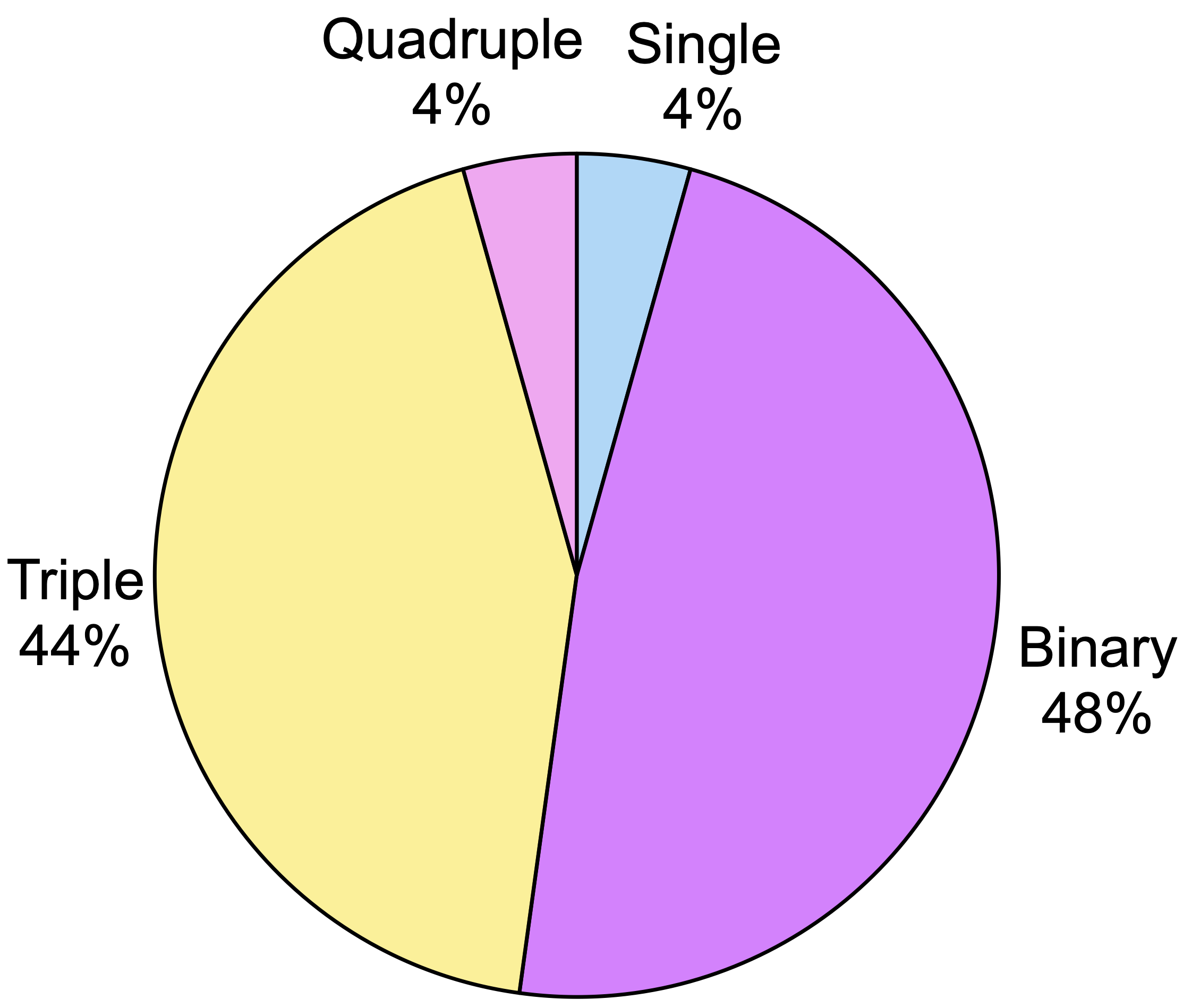
Figure 10: Pie-chart showing the multiplicity of our entire B star sample, taking into account spectroscopic, interferometric and Gaia eDR3 companions. This chart excludes stars for which there are conflicting results in the literature for the presence of a spectroscopic companion or those with a a lack of spectroscopic data to search for such a companion, meaning that these percentages are calculated for a sub-sample of 23 sources, rather than the total 32.

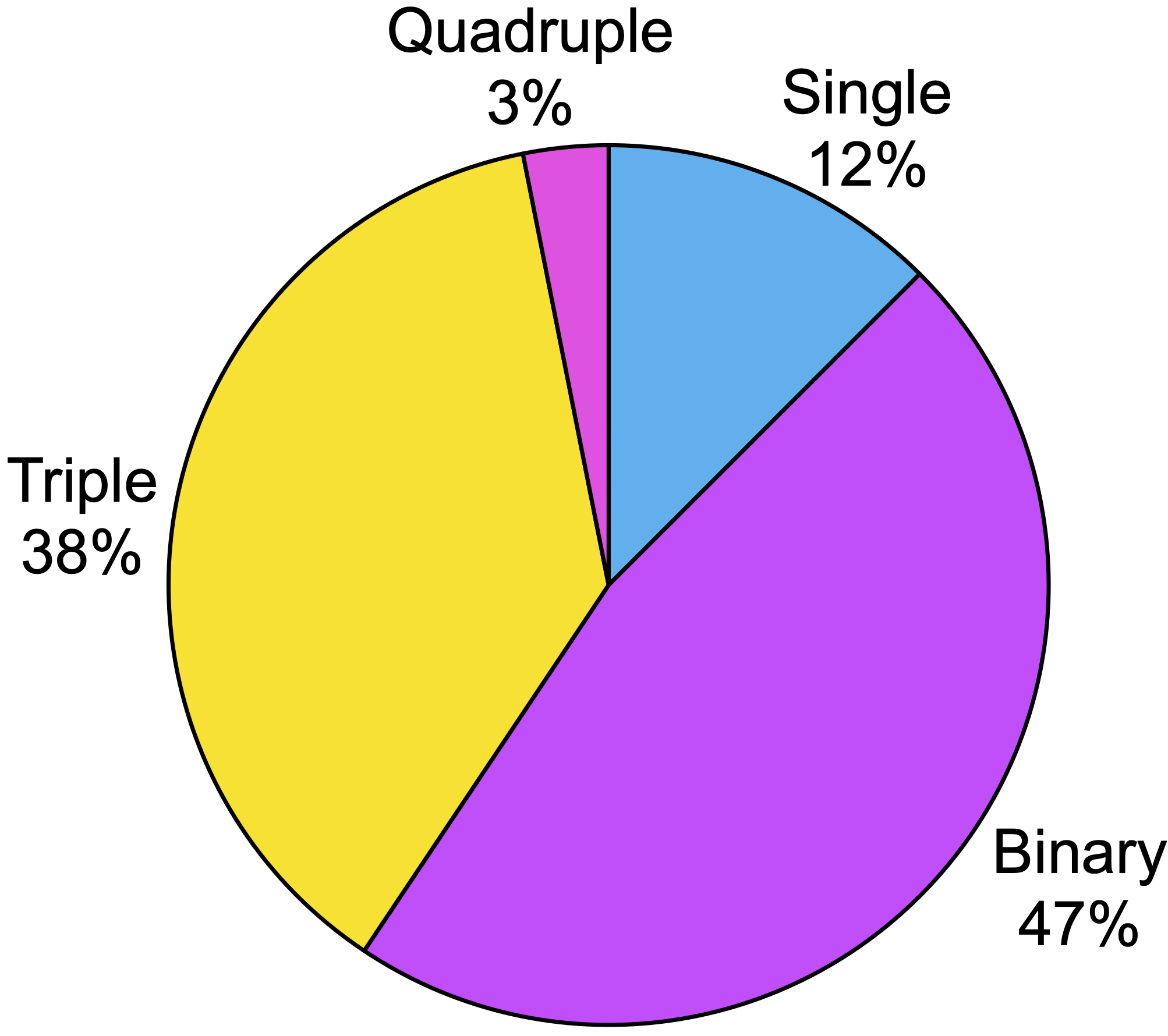
Figure 11: Pie-chart showing multiplicity of our entire B star sample of 32 sources, taking into account spectroscopic, interferometric and Gaia eDR3 companions.

Table 4: The results of the literature search for spectroscopic and/or long period companions. Starred sources are those whose companions are on long enough orbits to overlap with the interferometric detection range.

	Name	Reference	Notes
Clear detections	∗HD 25558	Sódor et al. (2014)	$P$=8.9$\pm$0.5yr
	HD 30836	Luyten (1936), Mahy et al. (2022)	$P$=9.5191d, P=9.519999$\pm$0.000409d
	∗HD 35337	Abt et al. (1990)	$P$=106.7$\pm$0.4d
	HD 37017	Leone & Catanzaro (1999)	$P$=18.6556$\pm$0.0017d
	∗HD 105382	Kervella et al. (2019)	$R_{orbit}$ from Gaia DR2 - 2.469 au
	HD 116658	Harrington et al. (2016)	$P$=4.0145d
	HD 140008	Thackeray & Hutchings (1965)	$P$=12.26d
	HD 161701	Hube (1969)	$P$=12.4520d
	HD 189103	Wilson (1921)	$P$=2.1051d
	∗HD 205637	Rivinius et al. (2006)	$P$=128.5d
	∗HD 212571	Bjorkman et al. (2002)	$P$=84.07$\pm$0.02d
	∗HD 224990	González & Levato (2009)	$P$=1740$\pm$22d
	∗MCW 1019	Irrgang et al. (2016b)	$P$=2245${}^{+25}_{-30}$d
	$\tau$ Lib	Pourbaix et al. (2004)	$P$=3.29d
Non-detections	HD 3379	Abt & Cardona (1984)
		Abt et al. (1990)
		Telting et al. (2006)
	HD 16582	Abt et al. (1990)
	HD 34816	Telting et al. (2006)
	HD 121743	Brown & Verschueren (1997)
		Shatsky & Tokovinin (2002)
		Telting et al. (2006)
	HD 132058	Brown & Verschueren (1997)
		Telting et al. (2006)
	HD 147932	Brown & Verschueren (1997)
		Rosslowe & Crowther (2018)
	HD 178175	Abt & Cardona (1984)
	HD 191263	Abt & Cardona (1984)
	HD 212076	Percy & Lane (1977)
		Hanuschik (1987)
		Chauville et al. (2001)
Conflicting results	HD 109026
	$\gamma$ Peg
	HD 66765
	HD 35149
	HD 51480
	HD 32249
Lack of data	HD 133518
	HD 67621
	HD 193933

Table 5: Wide binaries found in the Gaia eDR3 database for the entire sample. $\rho$ is the projected orbital separation.

Name	Gaia primary	Gaia companion	$\Delta\theta$	$\Delta\varpi\pm\sigma_{\Delta\varpi}$	$\Delta\mu\pm\sigma_{\Delta\mu}$	$\rho$
	Gaia EDR3 name	Gaia EDR3 name	(arcsec)	(mas)	(mas year-1)	(a.u.)
HD 121743	6110381256839901440	6110394073027855360	293.3	$0.049\pm 0.279$	$0.972\pm 0.424$	41302.0
		6110385929769619328	634.1	$0.067\pm 0.276$	$0.702\pm 0.404$	89314.1
HD 37017	3209634905754969856	3209634905754971136	22.8	$0.178\pm 0.155$	$0.67\pm 0.116$	8175.8

3.3.1 The prevalence of triple systems

The most likely expected configuration of stars in a bound triple system consists of a close inner binary and a tertiary companion at much larger separation that orbits the centre of mass of the inner binary. Such a system is referred to as a ‘hierarchical’ triple system (Evans, 1968). This is expected to be the most common form of triple system, as if the inner and outer orbits have similar radii, the system can become dynamically unstable leading to a star being ejected from the system (Kiseleva et al., 1994). One of the most commonly used tests to determine whether a triple system is stable is that of Mardling & Aarseth (1999). However, this calculation requires inclination and eccentricity information for the systems, which we do not possess for most of our sample.

Looking at the separations of our sample of interferometric candidate triples alone, we find separation ratios of 58%, 9%, 9%, 40% and 37% between the separation of the binary companion and the primary and the separation of tertiary and the primary. Therefore two systems have ratios less than 15%, making them likely hierarchical triples. The remaining three interferometric triples are systems that have separation ratios between 15-55% making their fates more uncertain without more orbital information. The timescale for an unstable system is about 30 times the inner binary period (Grishin et al., 2017), which is in turn much smaller than the expected lifetimes of these systems. It is statistically highly improbable that the majority of the comparable-separation triple systems we observe are actually unstable. Instead, it is likely that apparent non-hierarchical triples are due to projection effects, and that most, and likely all of the systems are in a stable, hierarchical configuration. Orbital monitoring of all these triple systems will allow us to decipher which systems may be on the precipice of collapse from those which are more stable and to eliminate any projection effects, but this is outside the scope of this paper.

By observing a sample of 165 spectroscopic binaries with follow-up NACO imaging, Tokovinin et al. (2006) found that short period binaries often have outer companions (63%$\pm$5% after incompleteness corrections) with 96% of their sample having an outer companion if the period of the inner binary was below 3d and 34% for periods greater than 12d. This was for a sample of solar-type stars, whose observed multiplicity and companion fractions are expected to be lower on average than B-type stars. We used the information compiled to calculate our ‘complete’ multiplicity fraction to compare with their work. Of our sample only HD 189103 and $\tau$ Lib have spectroscopic companions with periods of 3d or less (the former has no outer companion and the latter has one interferometric companion), but this is extreme low-number statistics so we do not expect agreement with Tokovinin et al. (2006).

3.4 Notes on specific sources and types of star

3.4.1 HD 51480

When fitting single star models to our datasets, we fit the diameter of the uniform disk instead of fixing it such that it could be modelled as an unresolved point source (0.2 mas). The majority of the sources fit with single star models converged on uniform disk values of 0.5 mas or lower. However, HD 51480 is much more extended with a fit diameter of 1.38${}^{+0.03}_{-0.08}$mas, corresponding to $\sim$1 au in diameter given the source’s distance. This is consistent as the decreasing visibility profile is typical of an extended structure. Additionally, spectra from Murphy et al. (2020) note the presence of P-Cygni profiles which could imply the presence of a hypergiant star. However, deviations from the smooth curve typical of a disk led us to also try multiple companion models for the system. In these cases, leaving the diameter of the primary free was unsuccessful, as the model could not converge. A binary model formed of two point sources can also fit the data well, with the secondary companion having comparable flux to the primary within errors (0.92$\pm$0.16) and very small separation (0.6995$\pm$0.046). However, this did not improve the fit to the data recorded across the K0G1 baseline (see Figure A.3). The system was classified as a Be star by Bidelman & MacConnell (1973). Wang et al. (2018) included the source in their candidates for Be and sub-dwarf O-star systems, but the signal associated with the system did not pass their selection criterion for further study. We also did a triple fit to see if we see any hints of a faint, more distant companion. A triple model with secondary fixed as described improved the fit, but the tertiary companion was below our calculated detection limit as well. Therefore, we choose a single star fit as the final model.

3.4.2 Be stars

Classical Be stars, as their name suggests, show strong emission lines which are associated with rapid rotation, circumstellar decretion discs generated as a result of this rotation and non-radial pulsations (e.g. Struve 1931, Rivinius et al. 2013). The Be star phase is observed to be transient and at least $\sim$20% of B-type stars are observed in this form. The multiplicity of Be stars is important to understand their nature as one major potential cause of their rapid rotation is binary interaction, although the exact percentage is still debated (e.g. van Bever & Vanbeveren 1997, Pols et al. 1991, Hastings et al. 2021). The binary formation channel assumes that two MS stars are in a close binary orbit, with one star being more massive than the other. The more massive star will swell first, overfill its Roche Lobe and transfer mass to the other star. This transfer spins up the second star, and eventually only the He core of the (originally) more massive stars remains. This He star is then likely to go through a SNe event which may result in the formation of a Be X-ray binary.

Within the sample there are 6 stars that have been reported to be Be stars. The Be stars in our sample show a range of multiplicities. Considering the ‘complete’ multiplicity fraction, 5 of the systems are binaries and the remaining system is single. Two of the binaries, HD 105382 and HD 178175 are interferometric, whilst the remaining systems are binaries thanks to spectroscopic companions. We measure a separation for the companion of HD 105382 of $\sim$37 mas, corresponding to $\sim$4 au given the source’s distance, and $\sim$5 mas/$\sim$2 au for HD 178175.

The remaining binary Be systems are HD 205637, HD 212571 and HD 212076. Klement et al. (2019) find a turn-down in the SED of HD 205637 which indicates a binary companion and Rivinius et al. (2006) also find it to be a binary. BeSS spectra of this system show strong double-peaked emission and narrow lines, implying that if this is a classical Be system, we view it close to edge on.

HD 212571 (also known as pi Aqr) is one of the most famous Be stars, a spectroscopic binary system and an irregular target. The source has been the subject of much study in the literature, with numerous spectra taken and the source also being present in the BeSS catalogue (Neiner et al., 2011). Spectroscopically there have been a number of comments on its multiplicity. Bjorkman et al. (2002) propose that, based on trailing H-$\alpha$ emission and radial velocity variations, the source could be a binary system with a period of $\sim$84 days and Langer et al. (2020) note that this companion could be a stripped star. If this is indeed a signal from the companion, the orbit is relatively long. However, Klement et al. (2019) find no evidence of a companion in the study of the source’s SED and Wang et al. (2018) and Horch et al. (2019) find no indication of a companion in their spectra. During the fitting process, we found that a model consisting of a single extended disc can fit the data of the source. When fitting the data of HD 212571 we were able to fit a binary model. The separation of the companion was easy to constrain and was very small ($\sim$0.15 mas/0.05 au on average). This separation could correspond to a companion in the spectroscopic range. However, the errors on the flux were large (¿80%) and varied greatly between epochs so we deemed a binary model unreliable and settled on a single star model, in agreement with Klement et al. (2019), Wang et al. (2018) and Horch et al. (2019).

The final Be star system is HD 51480, which we discussed in the previous subsection. Given that the system appears to have a large extended component, it is unclear where the Be signature is coming from in the system, since the predicted size of this extended component is much larger than the predicted sizes of Be star discs (1 au vs. orders of stellar radii). Since the nature of the system is not clear, we do not discuss it as a Be star going forward.

3.4.3 Variable stars

Another common type of star within our B star sample are variable stars. A number of comments have been made in the literature between variability and multiplicity. One particularly discussed group of variable stars are classical Cepheid stars, which radially pulsate on rigid periods. Evans et al. (2005) postulated from Hubble UV spectra that the massive stellar system Y Car, which had been previously classified as a binary classic Cepheid, was in fact a triple system. Similarly a study of a sample of Galactic Cepheids with interferometric data by Gallenne et al. (2019) found several detections of companions.

The most prolific type of variable present in the sample are the $\beta$-Cep variables. The stars have masses $\gtrapprox$7 M_⊙ and exhibit minor, rapid variations in brightness (Lesh & Aizenman, 1978). Lefèvre et al. (2009) performed a study of the variability of 30% of the OB stars observed with HIPPARCOS and found that OBe stars were more variable than average, OB MS stars are less variable that average and that OB supergiants show average variability. This variation is thought to be due to pulsations at their surface driven by the kappa opacity mechanism (whereby high-opacity regions of partly ionised H and He in the stellar surface sink and rise in a cycle) and p-mode pulsations (radial pulsations caused by pressure waves travelling longitudinally that disturb the H and He material in stellar envelope, Lefèvre et al. 2009).

Eight of the stars in our sample are remarked to have variability in the literature. Two systems appear to be single, four are binaries and two are triple systems, so there are no clear trends between variability and the multiplicity of our sample.

A type of binary that can result in variability are eclipsing binaries, where stars within the system orbit in a plane that obstructs our line of sight. We searched the literature for evidence of eclipsing binaries within our sample. We find that three of our triple systems; HD 116658, HD 25558 (both from Lefèvre et al. 2009) and HD 35149 (IJspeert et al., 2021) have been categorised as eclipsing binaries. Lefèvre et al. (2009) only tentatively describe HD 116658 as an eclipsing binary, stating a possible period of 4.014 d. This is almost identical to the period of the spectroscopic companion detected around the system by Shobbrook et al. (1972) and we tentatively assume this spectroscopic companion is the secondary star we detect with interferometry. Lefèvre et al. (2009) define a period of 1.532d for HD 25558. A spectroscopic companion again exists for this system, but it has a long period and thus is more likely our interferometrically detected companion. IJspeert et al. (2021) note the presence of an eclipsing binary with a 2.28d period for the system HD 35149. Sódor et al. (2014) find a long-period spectroscopic companion which we suggest is the companion we detect interferometrically. Therefore, it seems that taking into account the eclipsing companion, the system could in fact be a triple, and we include it as such in our ‘complete’ multiplicity fraction plots and calculations (Section 3.3).

3.5 Comparison with other work

Using the results of Silaj et al. (2014) we attribute masses to the dwarf stars of our sample using their spectral sub-type. We omit the giants we observe given the large uncertainties associated with determining their stellar properties. Moe & Di Stefano (2017) collected the multiplicity statistics of a variety O, B and A stars by studying the data of a large number of sources using observations which covered much of the separation range of companions. They determine that at low masses the most likely form of stellar system is a single star system ($\sim$0.6), followed by a binary system ($\sim$0.3), then a triple system ($\sim$0.07) and a quadruple system ($\sim$0.01). As the mass of the system increases, these ratios change. Above $\sim$2 M_⊙, the binary system becomes the most probable. After $\sim$12 M_⊙ the triple becomes the most likely system and after $\sim$23 M_⊙ the quadruple is most probable. We find that the triples range in mass from $\sim$6-15 M_⊙. The binary mass range is 8-11 M_⊙. Only one dwarf system is a quadruple (with a estimated primary mass of 8 M_⊙). Of the dwarf star systems that we can compare with Silaj et al. 2014, the binaries have masses between 5.9-9.11 M_⊙ and the triples have masses between 5.9-13.21 M_⊙.

In order to compare the multiplicity fraction we derive with interferometry for B stars to a similar survey for O stars, we consider the SMaSH+ survey (Sana et al., 2014). This survey obtained high-angular resolution observations of $\sim$100 O-type stars across luminosity classes I-V for an average distance of 2 kpc. Like our work, one of the main SMaSH+ datasets is PIONIER data. After combining their results with known spectroscopic companions, they conclude that 91$\pm$3% of the O star systems they observe are multiple systems. This is in agreement with the complete multiplicity fraction we derive of 96$\pm$4% and the conclusion of the two works is the same - the majority of massive stars form in at least a binary system.

Recent work by Banyard et al. (2021) studied the multiplicity properties of B stars specifically in one open cluster NGC 6231. They determined a spectroscopic binary fraction for the cluster of 52$\pm$8% after bias correction, which is significantly lower than the fraction we derive for the cluster sources of our sample. However, this work probes a very different physical separation range to that we present here.

An interesting difference between our study and those we discuss above is the fact that the vast majority (SMaSH+) or all of the stars (Banyard et al., 2021) are in clusters or associations, whilst the majority of our B star sample is field stars. One previous study of binary systems in clusters, Hu et al. (2010), determined an early constraint on how a young star cluster’s binary fraction varies, determining that more binaries should be found towards the centre of clusters. Recent work by Deacon & Kraus (2020) used Gaia DR2 data to investigate the multiplicity of stars in the Alpha Per, Pleiades and Praesepe clusters. They find that the average separation of the wide binary systems is lower compared to the field binaries, implying that while some systems are able to persist, it is likely that the dynamically high processing cluster environment disrupts most wide binary systems. Given the increased gravitational potential wells of O-type stars, it is possible that for the cluster-member-heavy SMaSH+ sample, outer companions have been disrupted in the cluster environments and been removed, lowering their companion fraction.

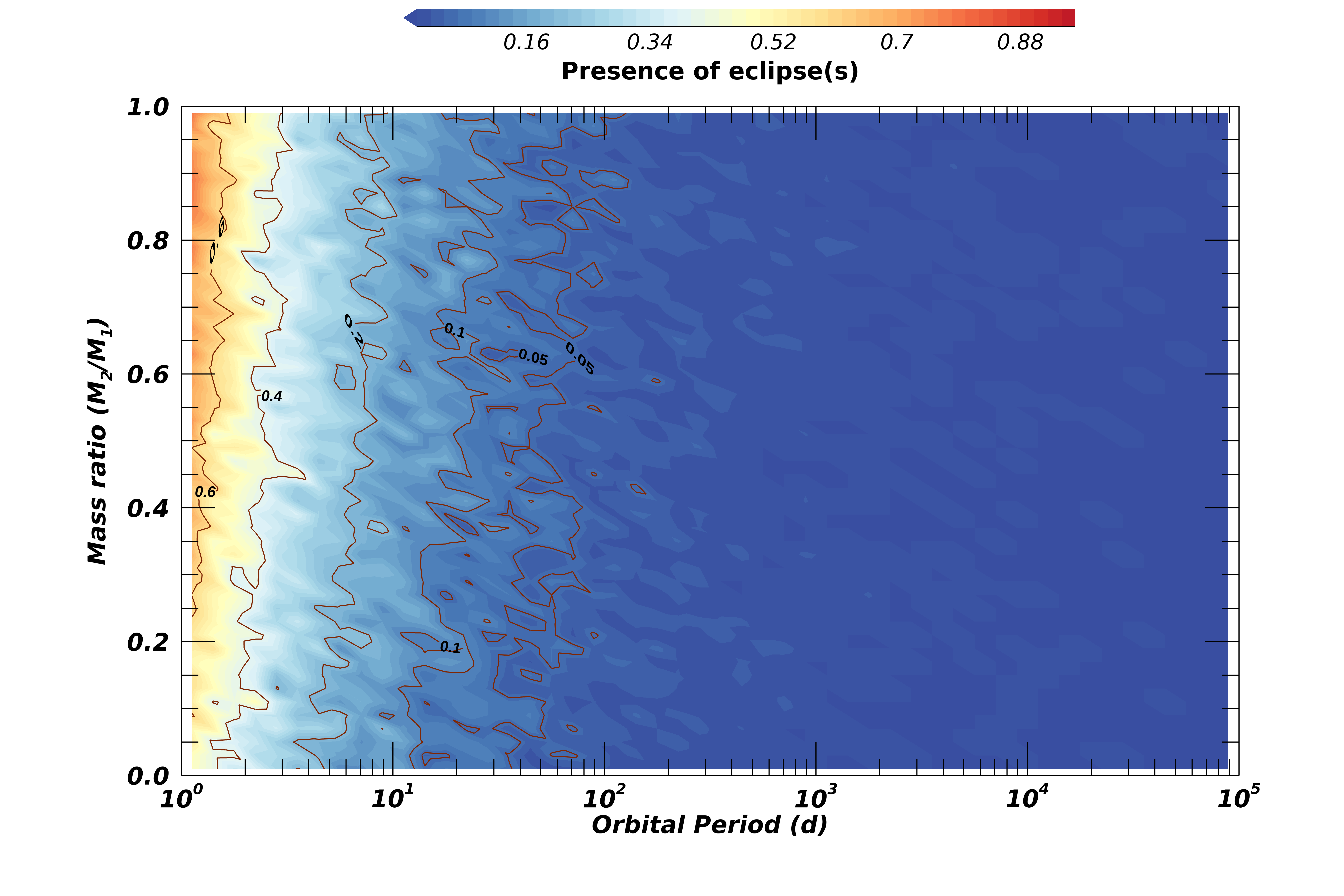
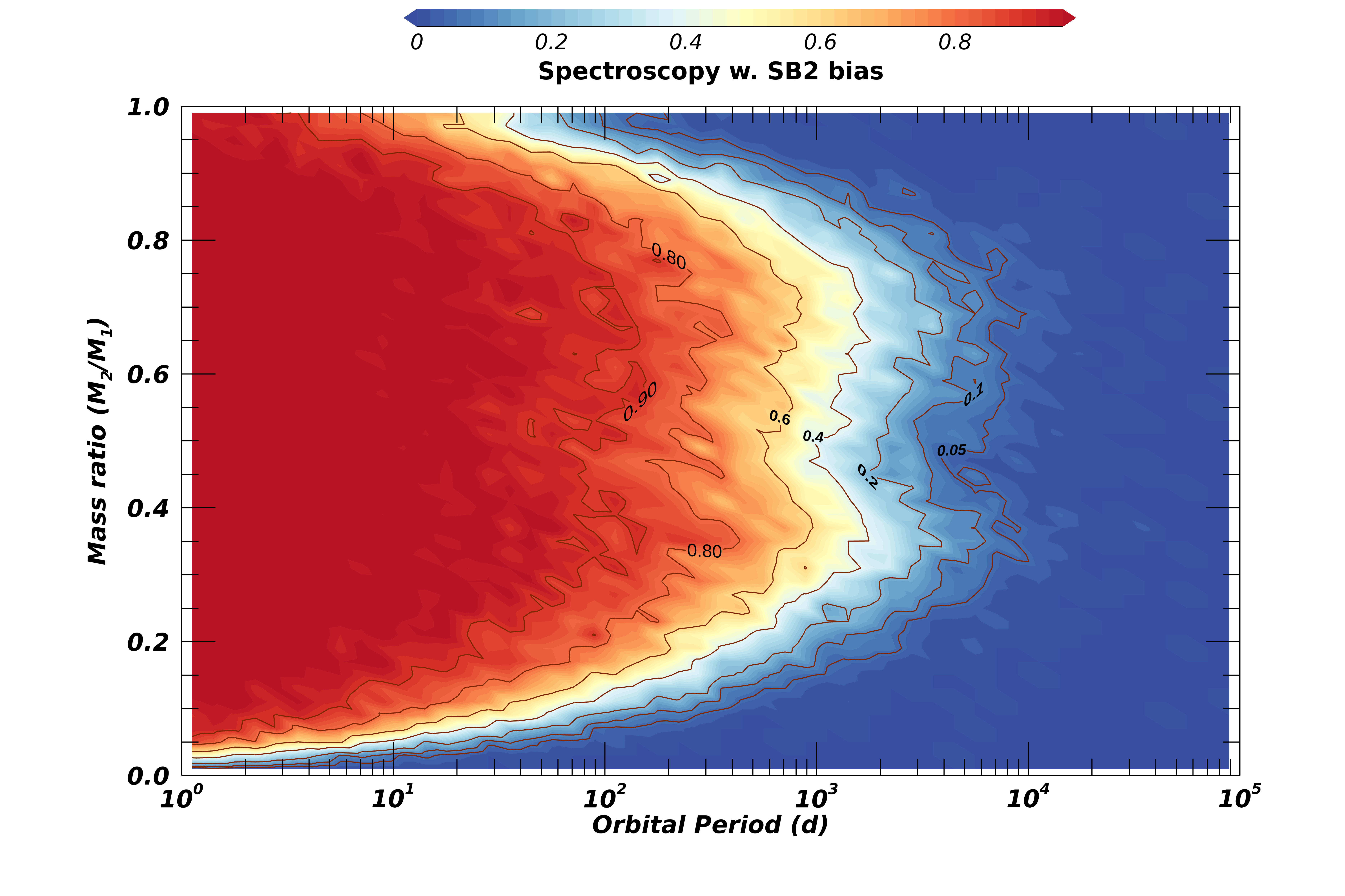
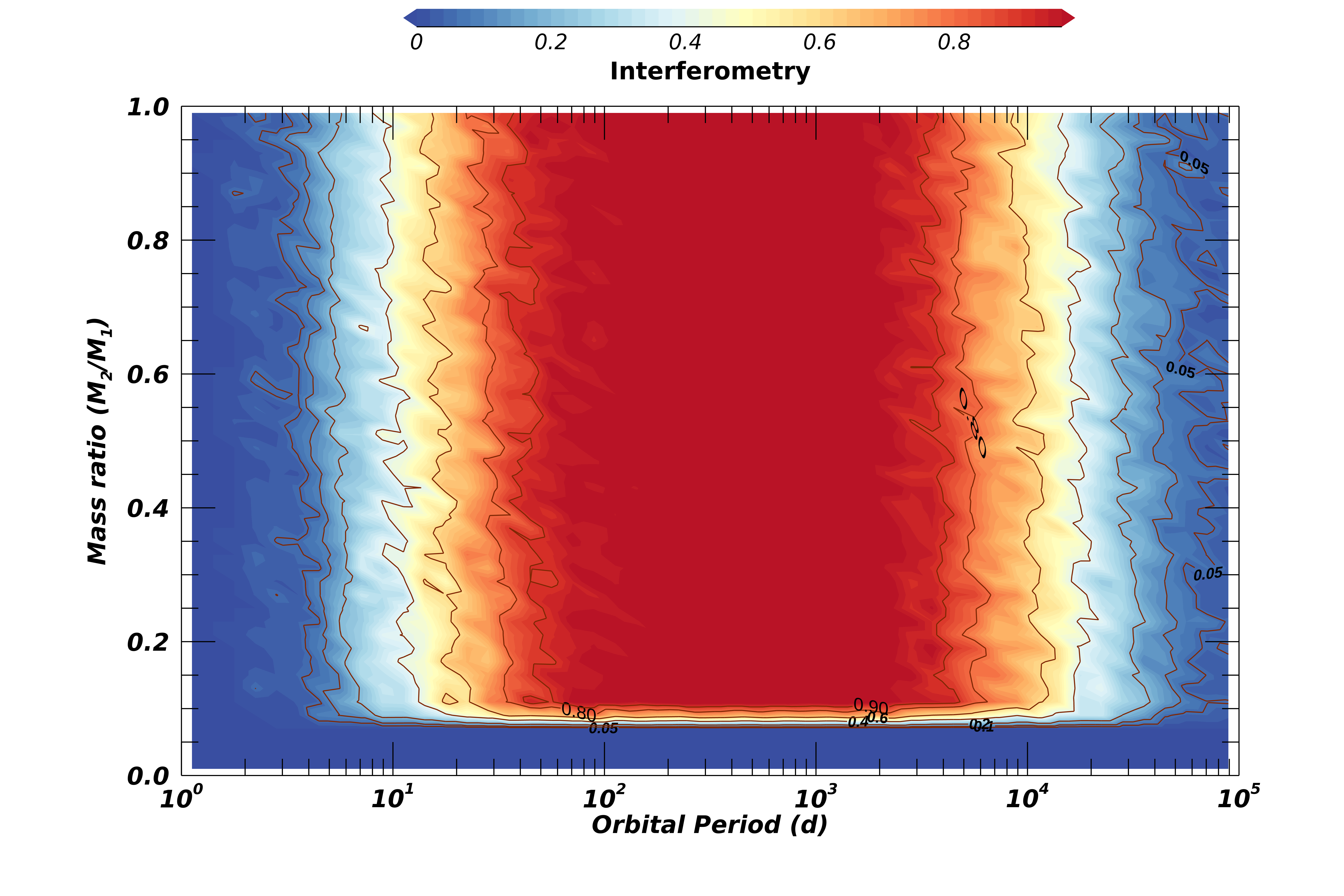
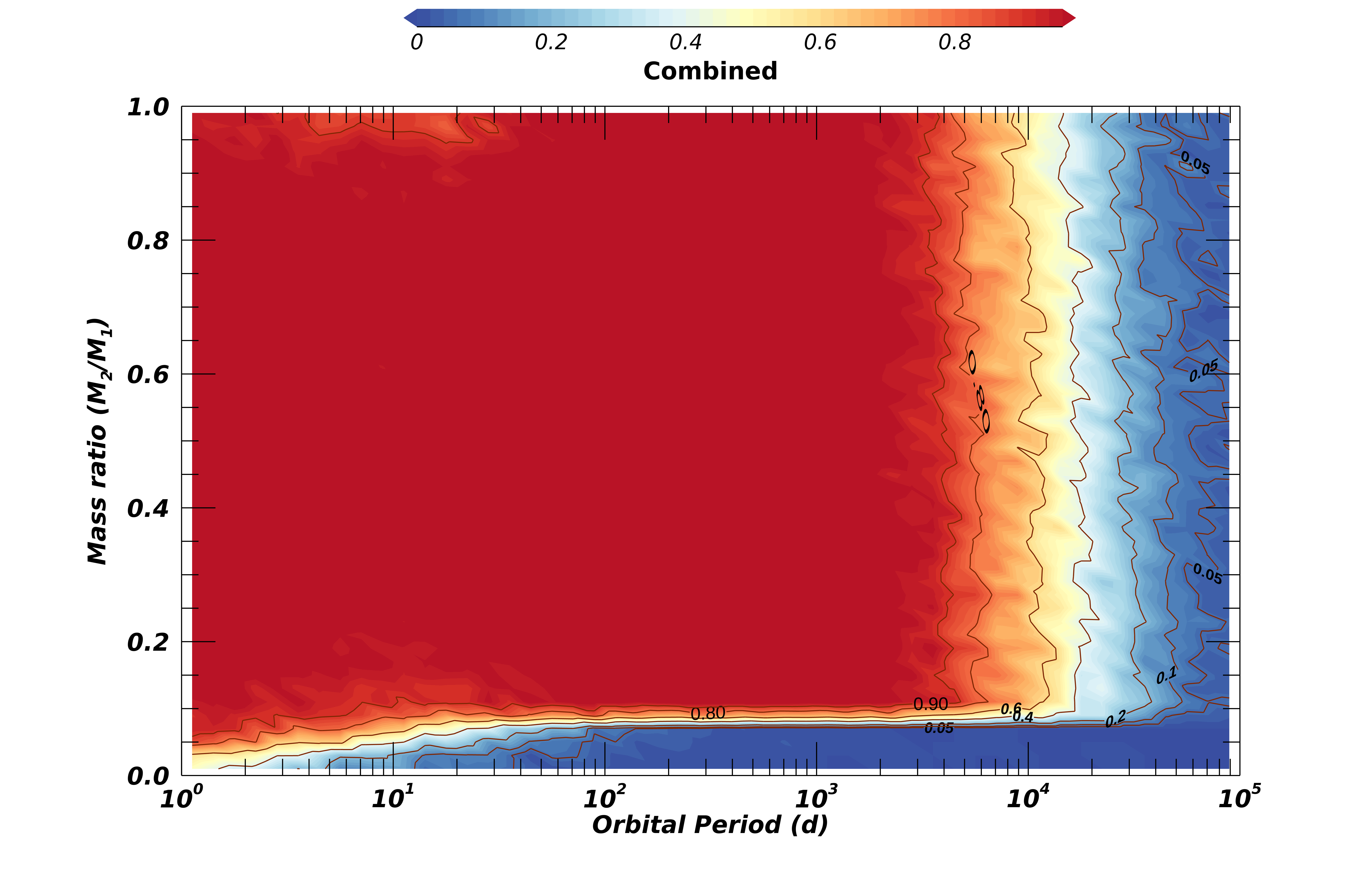
Figure 12: Detection probability of a binary system as a function of its orbital period $P$ and mass-ratio $q=M_{2}/M_{1}$.

4 Observational biases and companion detection capabilities

Our results so far are purely observational. In this section we evaluate the sensitivity of different techniques to detect companions to our B-type stars sample. In this exercise, we ignore the four supergiant stars that have different mass-luminosity and mass-radius relation to the remaining 33 stars of the sample. This allows us to focus on the near-ZAMS multiplicity properties of B stars.

We use a Monte-Carlo approach to simulate artificial populations of B-type binaries (Sana et al., 2013; Bodensteiner et al., 2021) and we apply detection criteria specific to various binary detection techniques to evaluate the likelihood of detecting a companion as a function of various physical and orbital properties. We adopt the following input distributions: an Öpik-law for orbital periods, covering the range $\log P=0...5$, a uniform distribution for mass-ratios in the range $q=M_{2}/M_{1}=0.01...1.0$ and a power-law distribution $f_{e}\propto e^{-0.5}$ for eccentricities (Sana et al., 2012). Maximum eccentricities depend on the orbital period and are computed such that the separation at periastron is larger than 0.1 au. We also adopt random orientations of the orbital planes in the 3-dimensional space and random times of periastron passage. We use a global mass-radius relation to evaluate the presence of eclipses ($R=M^{0.72}$; Eker et al., 2018) and the mass-ratio – flux ratio relation $q=F_{H}^{0.7}$ of Sect. 3.2 to estimate the $H$-band flux ratio. For our simulations to closely represent our sample properties we draw the distances and masses from normal distributions centred on the values listed in Table 1, and use the respective uncertainties as 1$\sigma$ dispersions. We drew 10 000 populations of 33 main-sequence B-type binaries and investigated the detection of companions by simulated observing campaigns using three different techniques: interferometry, spectroscopy and photometry. Specific equations are given in Sana & Vrancken (2025). We limit our discussion to detectability as a function of orbital periods and mass-ratios as these are the dominant parameters in determining the detectability of a binary system. The sensitivity of the various detection methods, and combination thereof, are summarised in Fig. 12.

For interferometry, we simulate a single observational epoch, randomly placed along the orbit, and we compare the projected angular separation $\rho$ between the two components of the binary systems to the inner and outer working angles of PIONIER (resp, IWA and OWA). We consider a companion to be detectable if the projected separation satisfies $1\leq\rho/\mathrm{mas}\leq 100$ and the H-band flux ratio is larger than 3% as representative of the upper envelope of our 3$\sigma$ detection limit (Table 2). Figure 12 shows that the detection probability is very much independent of the mass-ratio down to the flux-contrast threshold of 3%, which sets a sharp limit a $q=0.085$. The period sensitivity range is mostly set by the distance of our targets and the IWA and OWA of PIONIER, resulting in a very homogenous, high ($>90$%) detection probability between 50 and 3000 days. The detection probability remains significant ($>50$%) from 15 to 10 000 days.

For spectroscopy, we simulate a representative observing campaign consisting of 10 observational epochs spread over 1000 days ($\approx$ 3 years) with a radial velocity (RV) precision of 3 km s^-1. We simulate measured RVs accounting for the blending of spectral lines using the dedicated line-blending simulations for medium-resolution spectroscopy of Banyard et al. (2021). We adopt a detection threshold at a peak-to-peak RV variation of at least 20 km s^-1 and with a variability confidence larger than 4$\sigma$ (e.g. Banyard et al. 2021). Spectroscopy is very sensitive at short periods ($>90$% for $P<90$ d), except for low mass- and high-mass ratios where the detection probability is impacted by insufficient reflex motion of the primary and by the SB2 line-blending bias, respectively. Spectroscopy remains sensitive up to periods of $\approx 1000$ days in favourable configurations.

While photometry is not the main source of information of the present study, we still include it in our simulations as, following Sana et al. (2025, in press), it is a straightforward addition to estimate the occurrence of eclipses for a given orbit and pair of stellar radii . We conservatively assume that any eclipse would lead to a detection independently of considerations on the quality of photometric campaign or the number of epochs. Our simulations confirmed that the bulk of eclipsing binaries is limited to orbital periods of a few days, but also that a small fraction of systems still show eclipses up to periods of a couple months.

The combination of these various techniques leads to a detection probability of 99% up to periods of 1000 days (96% up to 30 yr) and mass-ratio down to $\approx 0.1$. For the shortest period ($P<10$), 40% of the lowest mass-ratio systems ($q<0.1$) are avoiding detection, which is the main limitation to the overall 95%-detection probability in that period range. In the range 10-1000 d, the overall detection is of 91%, rising to 99% when ignoring systems with $q<0.1$. Given these high-detection probability, we consider that multiplicity fractions based on systems that have both interferometry and archival spectroscopy do not need bias-correction down to $q=0.1$ and periods of a few years.

For systems with insufficient spectroscopy, 1 to 3 companions with $q<0.1$ could have been missed (assuming a uniform mass-ratio distribution).

The set of 12 systems with insufficient or inconclusive spectroscopy (see Table 4) deserve further discussion as they may have undetected companions in the short-period range. Again ignoring the supergiants, seven objects out of 21 with ‘complete’ detections have companions with orbital periods $P<20$ days. Applying this occurrence rate of 0.3 to the 10 non-supergiants with missing or conflicting spectroscopic results, we could have missed three short period systems. Given the sample of main-sequence stars with insufficient spectroscopy is dominated by single (4) and binary (5) stars, these non-detection are likely to bring down the fraction of single stars from 19% to 15% and increase the triple fraction by about a same amount. However these corrections remain smaller than the statistical uncertainties which are of the order of 8-9% depending on whether supergiants are included or not. Therefore, we conclude that our determined multiplicity and companions fractions are reliable and, at worst, slightly underestimate the number of companions around the stars in our sample.

5 Conclusions

Using high-resolution H-band interferometric data from PIONIER/VLTI, we have probed the multiplicity of a sample of 32 B-type stars in the interferometric range. The sample consists mostly of field stars, with eight of the sample belonging to clusters or associations. We used parametric models using the code PMOIRED to fit the synthetic closure phases and squared visibilities from those models to the observed closure phases and visibilities obtained with PIONIER to determine the number of stars and their characteristics, primarily flux and separation.

Following this analysis, we determine an interferometric multiplicity fraction of 0.72$\pm$0.08 for this sample of stars. The most common form of multiple system detected is a triple system, with an overall interferometric companion fraction of 1.88$\pm$0.24 determined. Within our sample we, find that the majority of the companions detected lie between separations of 1-20 mas and have fluxes $<$30% the flux of the brightest star in the system. This implies that most of the companions to these stars are lower-mass, which is in agreement with the observed IMF.

We combine our interferometric results with spectroscopic companions and eclipsing binaries detected in the literature and wide companions statistically derived from Gaia eDR3 using the proper motions and distances of the stars surrounding our sources. Using simulations of B star multiples we determine that both our interferometric results and those from combined techniques are not strongly affected by observational biases. The ‘complete’ statistics results in multiplicity and companion fractions of 0.88$\pm$0.06 and 2.31$\pm$0.27 respectively for our sample, with many interferometric binaries becoming hierarchical triples thanks to the presence of a spectroscopic companion. Therefore, the multiplicity of B stars likely dominates their evolution and the role of tertiary companions in this process is likely also of significance.

Appendix A Plots and fits for each source

Below we present the observations, model fits and images and bootstrap error calculations for the entire sample of sources. Note that we do not include model images for the single star models, just their fits to the data and the bootstrap plots for the size of the uniform disks. The order of the sources matches Table 2.

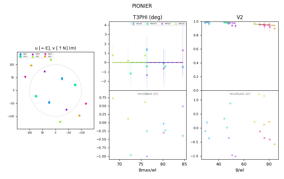
Figure 13: The best-fit data for HD 16582. On the left, the $u-v$ coverage from the observations with PIONIER can be seen. The different colours correspond to the telescope pair with which that particular data was acquired at the VLTI. In the middle, the closure phase (T3PHI) fit and residuals are shown in terms of the spatial frequency (B_avg/$\lambda$, written as Bavg/wl on the axes). On the right, the fit to the squared visibilities (V2) and the associated residuals are shown, again in terms of spatial frequency. Across the two fits, the data are represented as points whilst the fit as a continuous line.

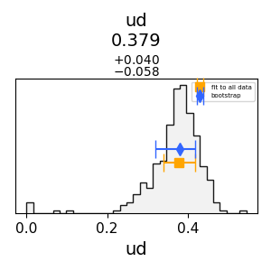
Figure 14: Bootstrapping plot showing the error determination for the dataset fit in Figure 13.

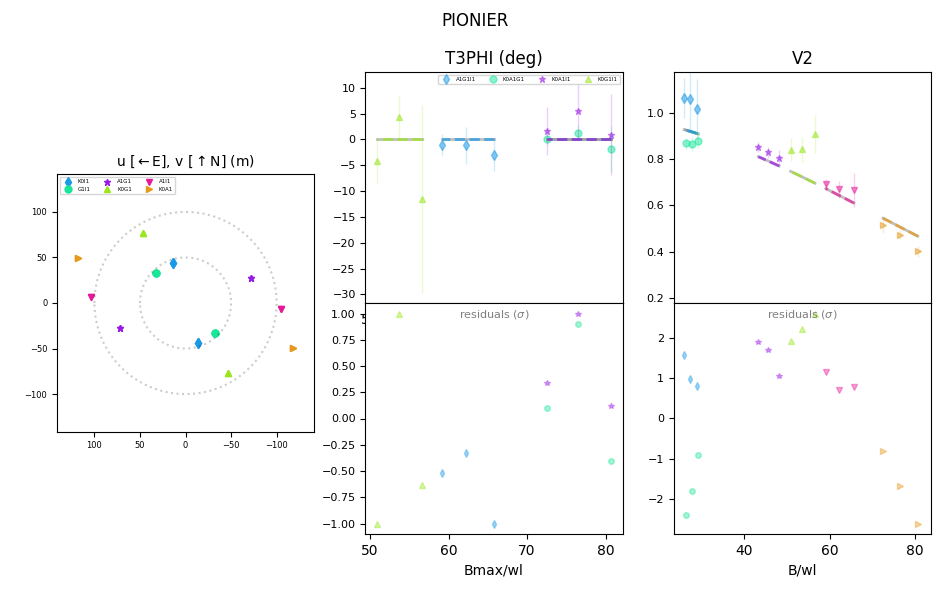
Figure 15: The best-fit data for HD 51480.

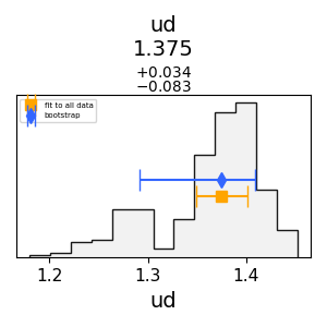
Figure 16: Bootstrapping plot showing the error determination for the dataset fit in Figure 15.

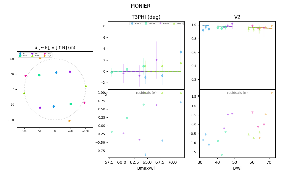
Figure 17: The best-fit data for HD 66765.

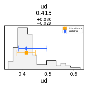
Figure 18: Bootstrapping plot showing the error determination for the dataset fit in Figure 17.

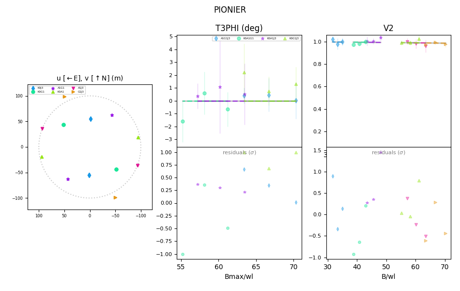
Figure 19: The best-fit data for HD 67621.

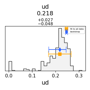
Figure 20: Bootstrapping plot showing the error determination for the dataset fit in Figure 19.

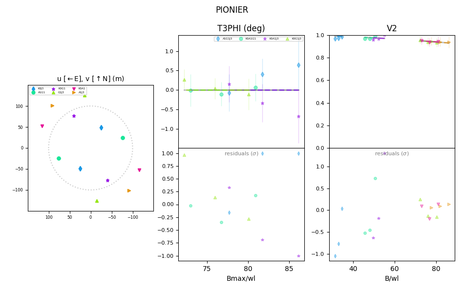
Figure 21: The best-fit data for HD 121743.

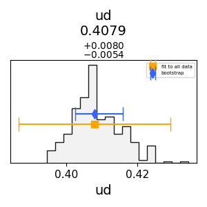
Figure 22: Bootstrapping plot showing the error determination for the dataset fit in Figure 21.

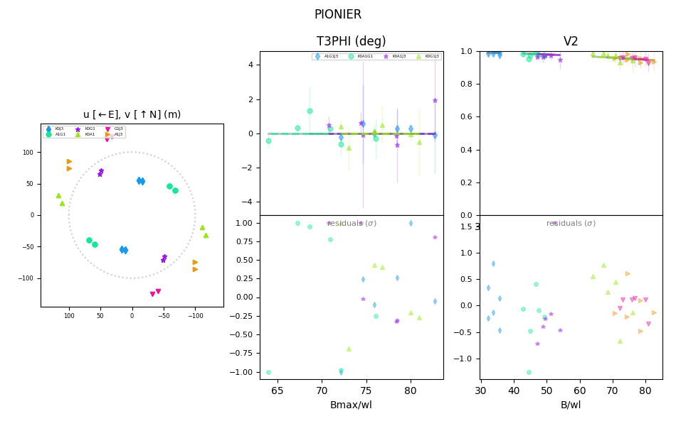
Figure 23: The best-fit data for HD 189103.

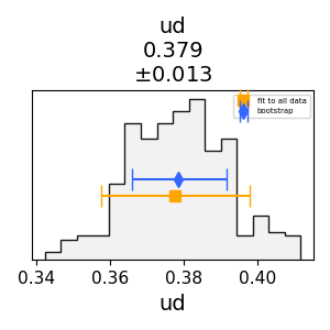
Figure 24: Bootstrapping plot showing the error determination for the dataset fit in Figure 23.

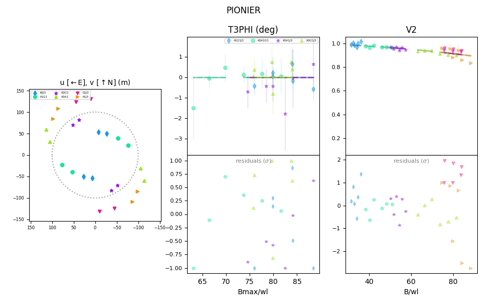
Figure 25: The best-fit data for HD 205637.

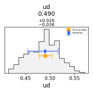
Figure 26: Bootstrapping plot showing the error determination for the dataset fit in Figure 25.

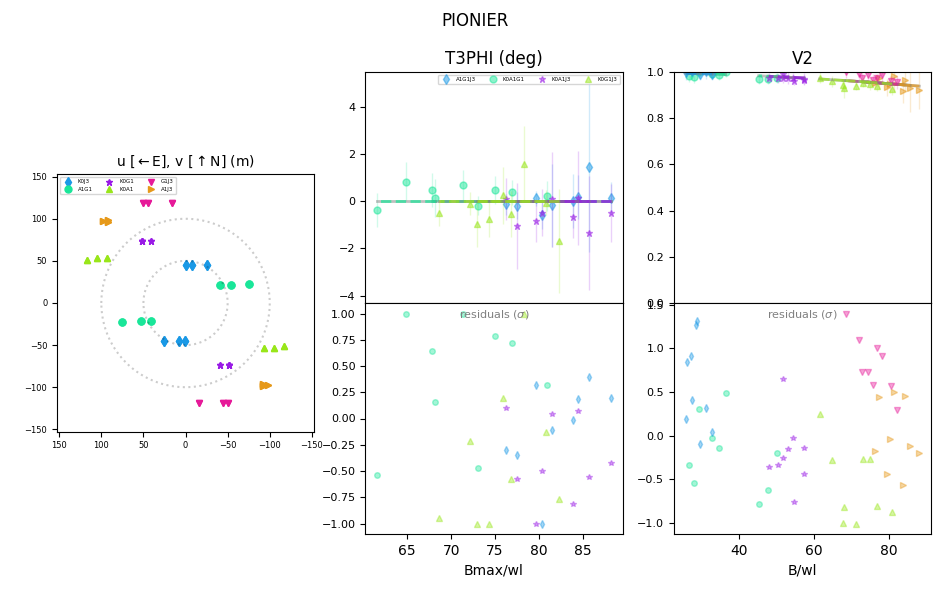
Figure 27: The best-fit data for HD 212571.

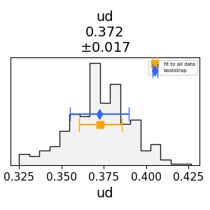
Figure 28: Bootstrapping plot showing the error determination for the dataset fit in Figure 27.

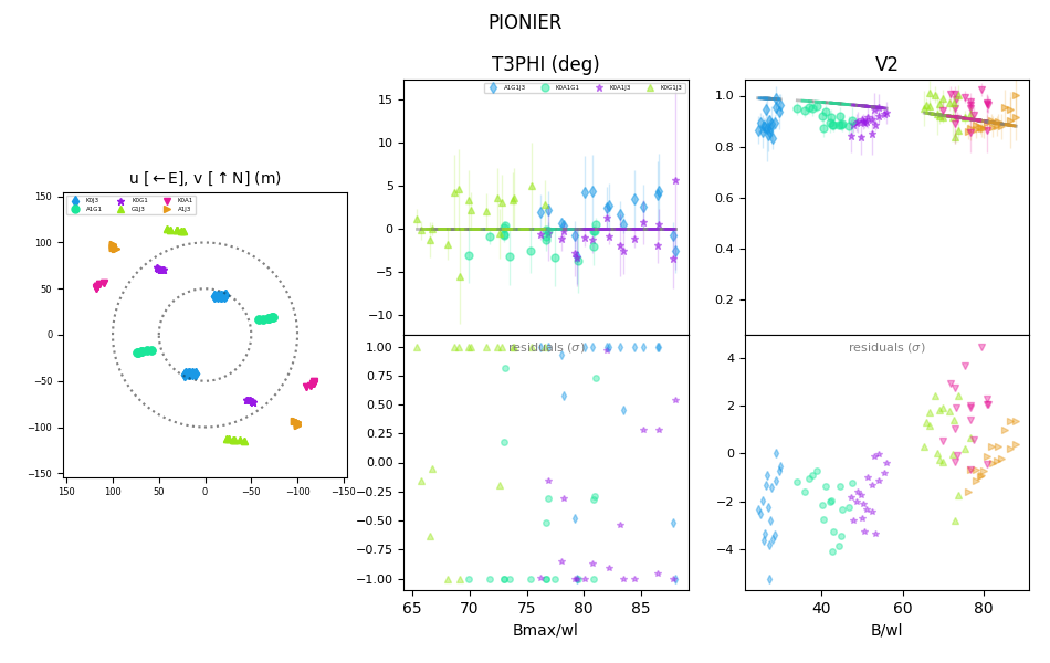
Figure 29: The best-fit data for MCW 1019.

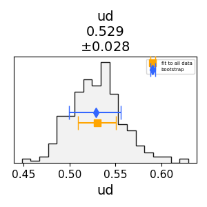
Figure 30: Bootstrapping plot showing the error determination for the dataset fit in Figure 31.

Figure 31: The best-fit data for MCW 1019.

Figure 32: Bootstrapping plot showing the error determination for the dataset fit in Figure 31.

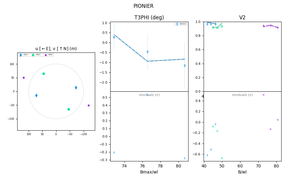
Figure 33: The best-fit data for $\gamma$ Peg. On the left, the $u-v$ coverage from the observations with PIONIER can be seen. The different colours correspond to the telescope pair with which that particular data was acquired at the VLTI. In the middle, the closure phase (T3PHI) fit and residuals are shown in terms of the spatial frequency (B_avg/$\lambda$, written as Bavg/wl on the axes). On the right, the fit to the squared visibilities (V2) and the associated residuals are shown, again in terms of spatial frequency. Across the two fits, the data are represented as points whilst the fit as a continuous line.

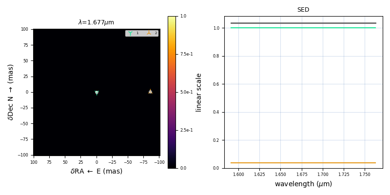
Figure 34: Model image created based on the best-fitting model of $\gamma$ Peg.

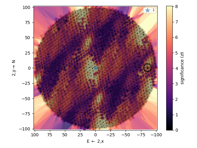
Figure 35: Plot showing the grid search used to search for the companion around $\gamma$ Peg and the companion’s significance.

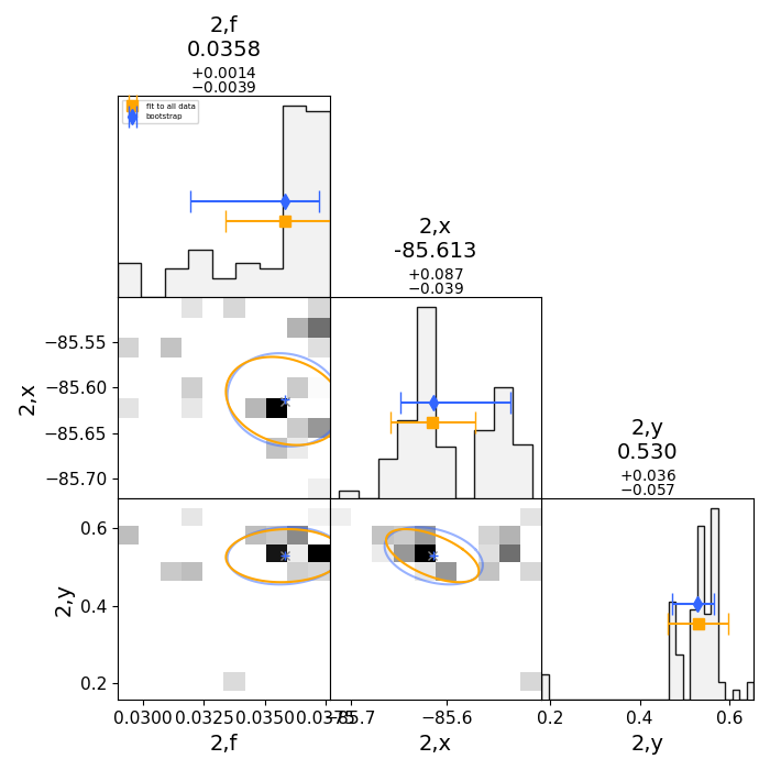
Figure 36: Bootstrapping plot showing the error determination for the dataset of $\gamma$ Peg.

Figure 37: The best-fit data for $\gamma$ Peg. On the left, the $u-v$ coverage from the observations with PIONIER can be seen. The different colours correspond to the telescope pair with which that particular data was acquired at the VLTI. In the middle, the closure phase (T3PHI) fit and residuals are shown in terms of the spatial frequency (B_avg/$\lambda$, written as Bavg/wl on the axes). On the right, the fit to the squared visibilities (V2) and the associated residuals are shown, again in terms of spatial frequency. Across the two fits, the data are represented as points whilst the fit as a continuous line.

Figure 38: Model image created based on the best-fitting model of $\gamma$ Peg.

Figure 39: Plot showing the grid search used to search for the companion around $\gamma$ Peg and the companion’s significance.

Figure 40: Bootstrapping plot showing the error determination for the dataset of $\gamma$ Peg.

Figure 41: The best-fit data for HD 3379. On the left, the $u-v$ coverage from the observations with PIONIER can be seen. The different colours correspond to the telescope pair with which that particular data was acquired at the VLTI. In the middle, the closure phase (T3PHI) fit and residuals are shown in terms of the spatial frequency (B_avg/$\lambda$, written as Bavg/wl on the axes). On the right, the fit to the squared visibilities (V2) and the associated residuals are shown, again in terms of spatial frequency. Across the two fits, the data are represented as points whilst the fit as a continuous line.

Figure 42: Model image created based on the best-fitting model of HD 3379.

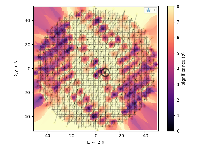
Figure 43: Plot showing the grid search used to search for the companion around HD 3379 and the companion’s significance.

Figure 44: Bootstrapping plot showing the error determination for the dataset of HD 3379.

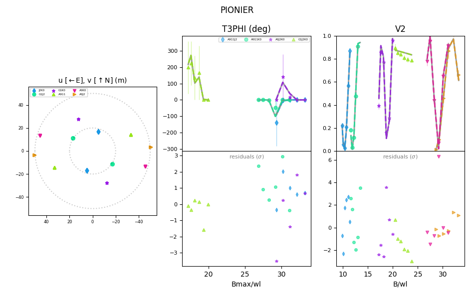
Figure 45: The best-fit data for HD 25558. On the left, the $u-v$ coverage from the observations with PIONIER can be seen. The different colours correspond to the telescope pair with which that particular data was acquired at the VLTI. In the middle, the closure phase (T3PHI) fit and residuals are shown in terms of the spatial frequency (B_avg/$\lambda$, written as Bavg/wl on the axes). On the right, the fit to the squared visibilities (V2) and the associated residuals are shown, again in terms of spatial frequency. Across the two fits, the data are represented as points whilst the fit as a continuous line.

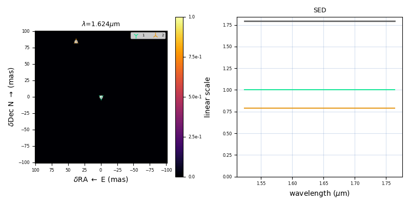
Figure 46: Model image created based on the best-fitting model of HD 25558.

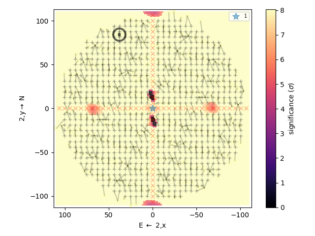
Figure 47: Plot showing the grid search used to search for the companion around HD 25558 and the companion’s significance.

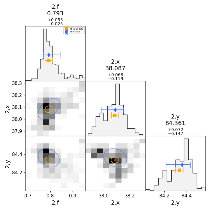
Figure 48: Bootstrapping plot showing the error determination for the dataset of HD 25558.

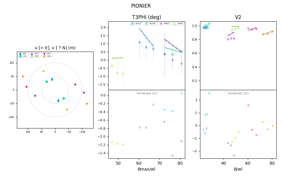
Figure 49: The best-fit data for HD 30836. On the left, the $u-v$ coverage from the observations with PIONIER can be seen. The different colours correspond to the telescope pair with which that particular data was acquired at the VLTI. In the middle, the closure phase (T3PHI) fit and residuals are shown in terms of the spatial frequency (B_avg/$\lambda$, written as Bavg/wl on the axes). On the right, the fit to the squared visibilities (V2) and the associated residuals are shown, again in terms of spatial frequency. Across the two fits, the data are represented as points whilst the fit as a continuous line.

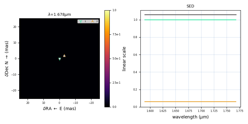
Figure 50: Model image created based on the best-fitting model of HD 30836.

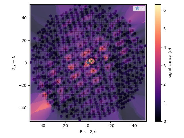
Figure 51: Plot showing the grid search used to search for the companion around HD 30836 and the companion’s significance.

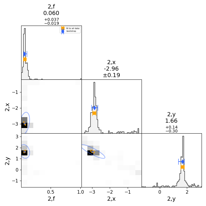
Figure 52: Bootstrapping plot showing the error determination for the dataset of HD 30836.

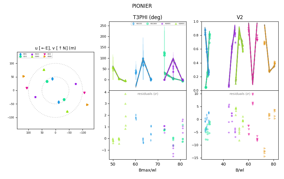
Figure 53: The best-fit data for HD 32249. On the left, the $u-v$ coverage from the observations with PIONIER can be seen. The different colours correspond to the telescope pair with which that particular data was acquired at the VLTI. In the middle, the closure phase (T3PHI) fit and residuals are shown in terms of the spatial frequency (B_avg/$\lambda$, written as Bavg/wl on the axes). On the right, the fit to the squared visibilities (V2) and the associated residuals are shown, again in terms of spatial frequency. Across the two fits, the data are represented as points whilst the fit as a continuous line.

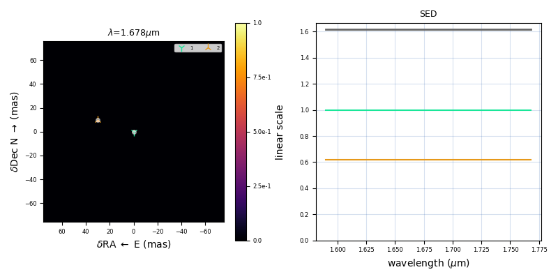
Figure 54: Model image created based on the best-fitting model of HD 32249.

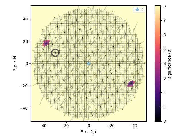
Figure 55: Plot showing the grid search used to search for the companion around HD 32249 and the companion’s significance.

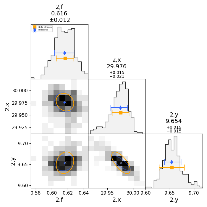
Figure 56: Bootstrapping plot showing the error determination for the dataset of HD 32249.

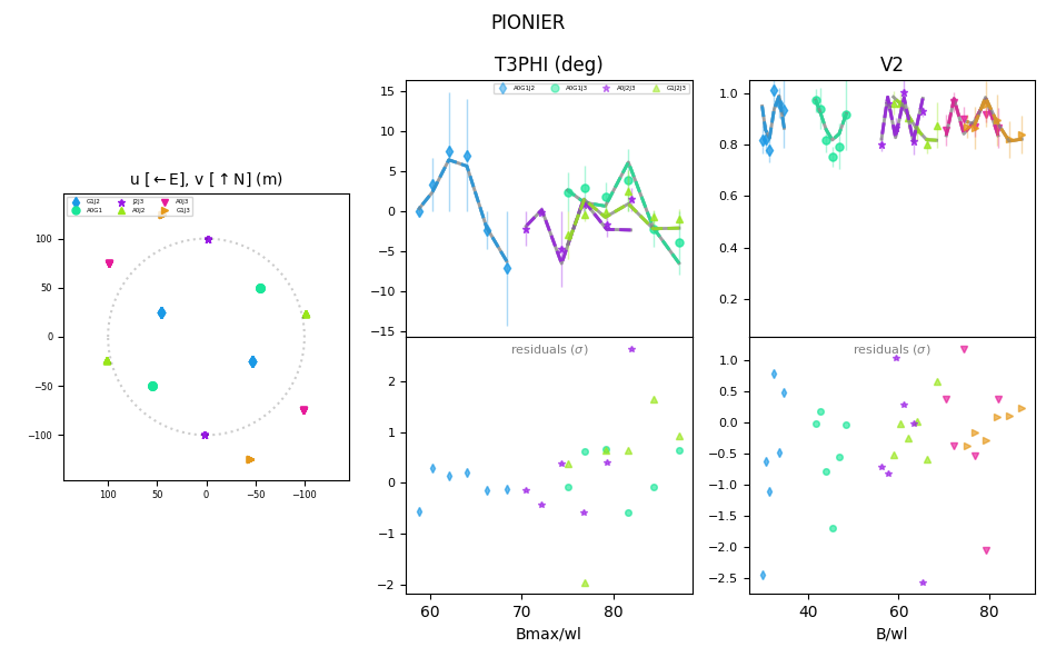
Figure 57: The best-fit data for HD 34816. On the left, the $u-v$ coverage from the observations with PIONIER can be seen. The different colours correspond to the telescope pair with which that particular data was acquired at the VLTI. In the middle, the closure phase (T3PHI) fit and residuals are shown in terms of the spatial frequency (B_avg/$\lambda$, written as Bavg/wl on the axes). On the right, the fit to the squared visibilities (V2) and the associated residuals are shown, again in terms of spatial frequency. Across the two fits, the data are represented as points whilst the fit as a continuous line.

Figure 58: Model image created based on the best-fitting model of HD 34816.

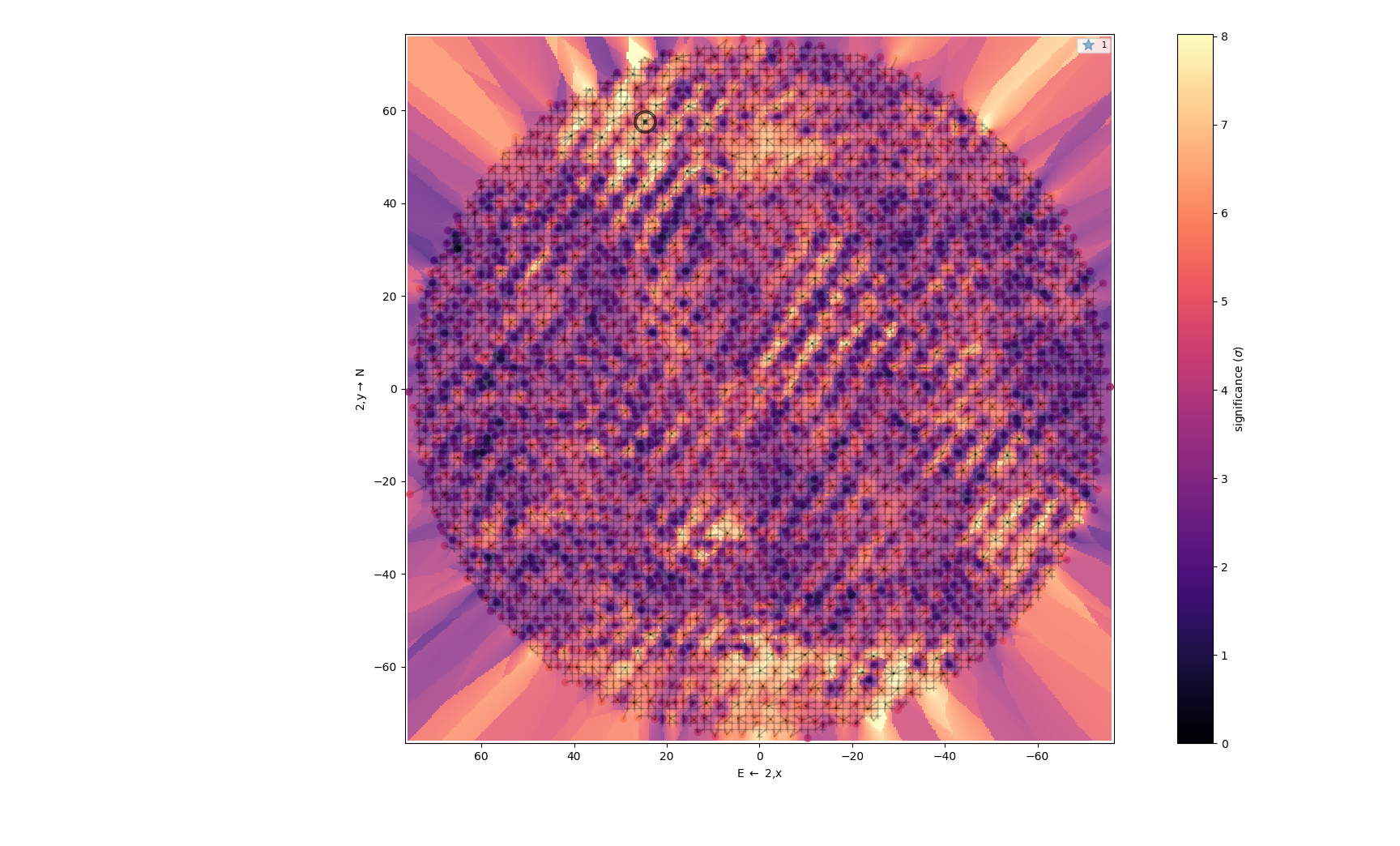
Figure 59: Plot showing the grid search used to search for the companion around HD 34816 and the companion’s significance.

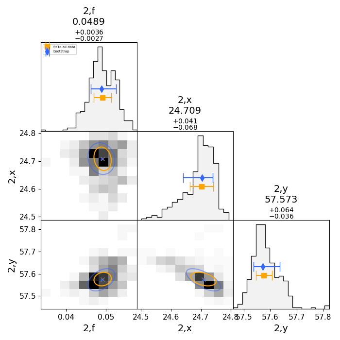
Figure 60: Bootstrapping plot showing the error determination for the dataset of HD 34816.

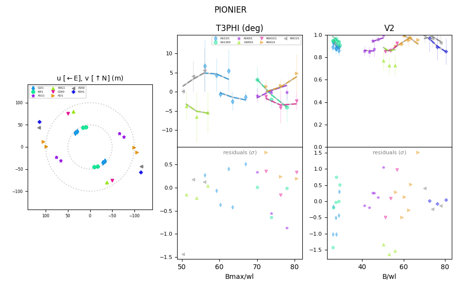
Figure 61: The best-fit data for HD 35337. On the left, the $u-v$ coverage from the observations with PIONIER can be seen. The different colours correspond to the telescope pair with which that particular data was acquired at the VLTI. In the middle, the closure phase (T3PHI) fit and residuals are shown in terms of the spatial frequency (B_avg/$\lambda$, written as Bavg/wl on the axes). On the right, the fit to the squared visibilities (V2) and the associated residuals are shown, again in terms of spatial frequency. Across the two fits, the data are represented as points whilst the fit as a continuous line.

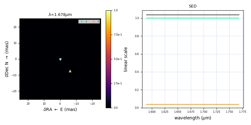
Figure 62: Model image created based on the best-fitting model of HD 35337.

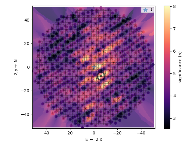
Figure 63: Plot showing the grid search used to search for the companion around HD 35337 and the companion’s significance.

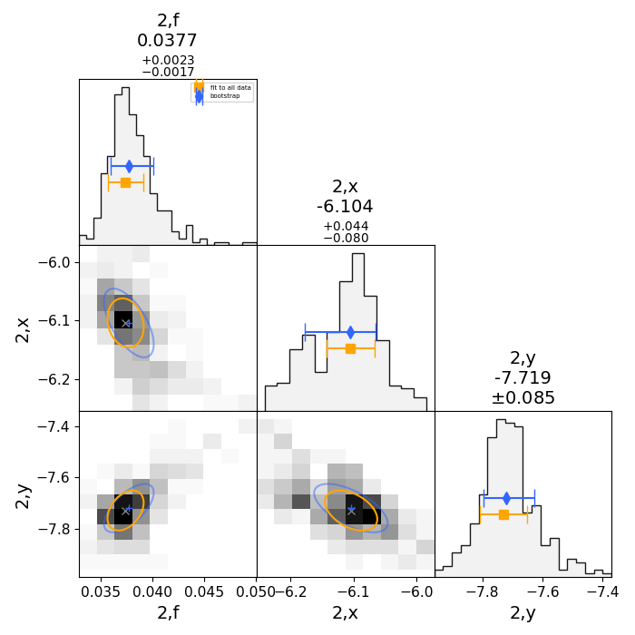
Figure 64: Bootstrapping plot showing the error determination for the dataset of HD 35337.

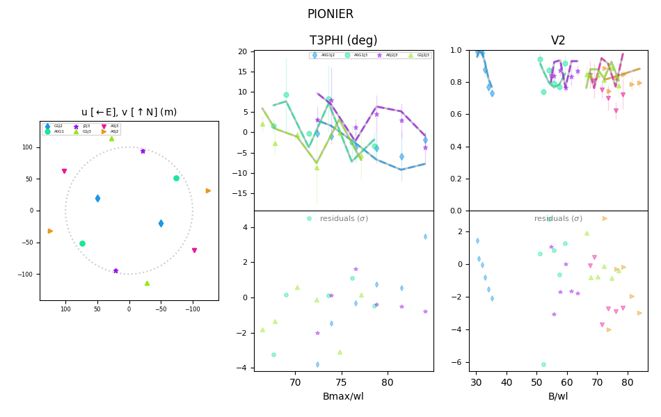
Figure 65: The best-fit data for HD 105382. On the left, the $u-v$ coverage from the observations with PIONIER can be seen. The different colours correspond to the telescope pair with which that particular data was acquired at the VLTI. In the middle, the closure phase (T3PHI) fit and residuals are shown in terms of the spatial frequency (B_avg/$\lambda$, written as Bavg/wl on the axes). On the right, the fit to the squared visibilities (V2) and the associated residuals are shown, again in terms of spatial frequency. Across the two fits, the data are represented as points whilst the fit as a continuous line.

Figure 66: Model image created based on the best-fitting model of HD 105382.

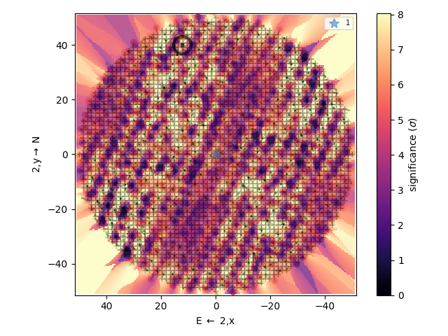
Figure 67: Plot showing the grid search used to search for the companion around HD 105382 and the companion’s significance.

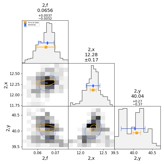
Figure 68: Bootstrapping plot showing the error determination for the dataset of HD 105382.

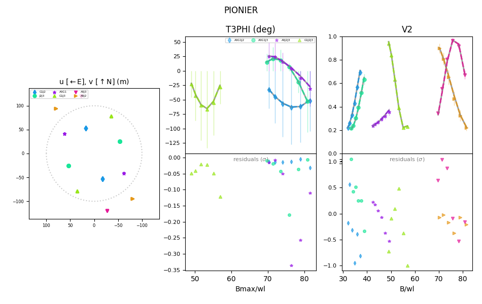
Figure 69: The best-fit data for HD 109026. On the left, the $u-v$ coverage from the observations with PIONIER can be seen. The different colours correspond to the telescope pair with which that particular data was acquired at the VLTI. In the middle, the closure phase (T3PHI) fit and residuals are shown in terms of the spatial frequency (B_avg/$\lambda$, written as Bavg/wl on the axes). On the right, the fit to the squared visibilities (V2) and the associated residuals are shown, again in terms of spatial frequency. Across the two fits, the data are represented as points whilst the fit as a continuous line.

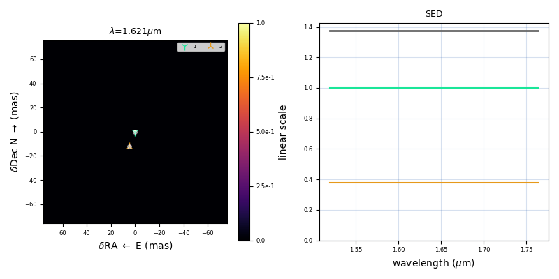
Figure 70: Model image created based on the best-fitting model of HD 109026.

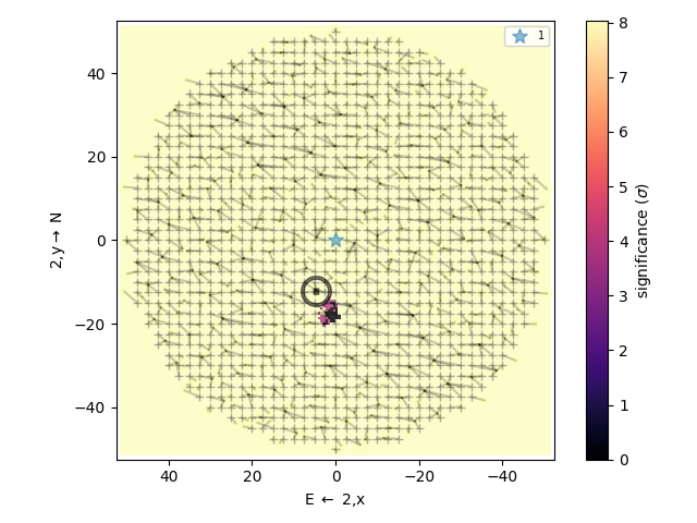
Figure 71: Plot showing the grid search used to search for the companion around HD 109026 and the companion’s significance.

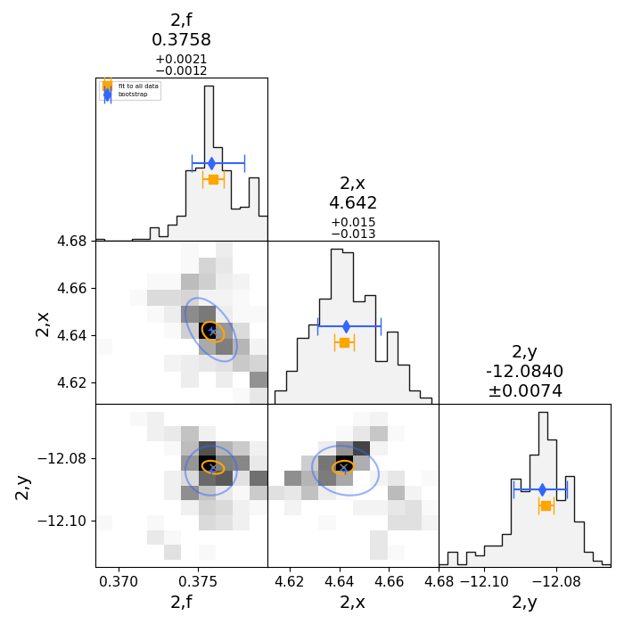
Figure 72: Bootstrapping plot showing the error determination for the dataset of HD 109026.

Figure 73: The best-fit data for HD 133518. On the left, the $u-v$ coverage from the observations with PIONIER can be seen. The different colours correspond to the telescope pair with which that particular data was acquired at the VLTI. In the middle, the closure phase (T3PHI) fit and residuals are shown in terms of the spatial frequency (B_avg/$\lambda$, written as Bavg/wl on the axes). On the right, the fit to the squared visibilities (V2) and the associated residuals are shown, again in terms of spatial frequency. Across the two fits, the data are represented as points whilst the fit as a continuous line.

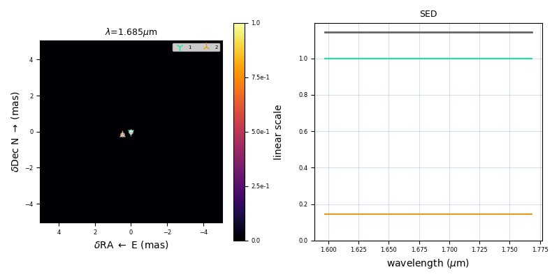
Figure 74: Model image created based on the best-fitting model of HD 133518.

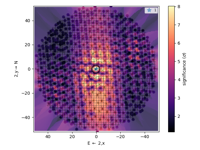
Figure 75: Plot showing the grid search used to search for the companion around HD 133518 and the companion’s significance.

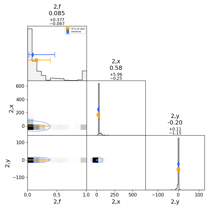
Figure 76: Bootstrapping plot showing the error determination for the dataset of HD 133518.

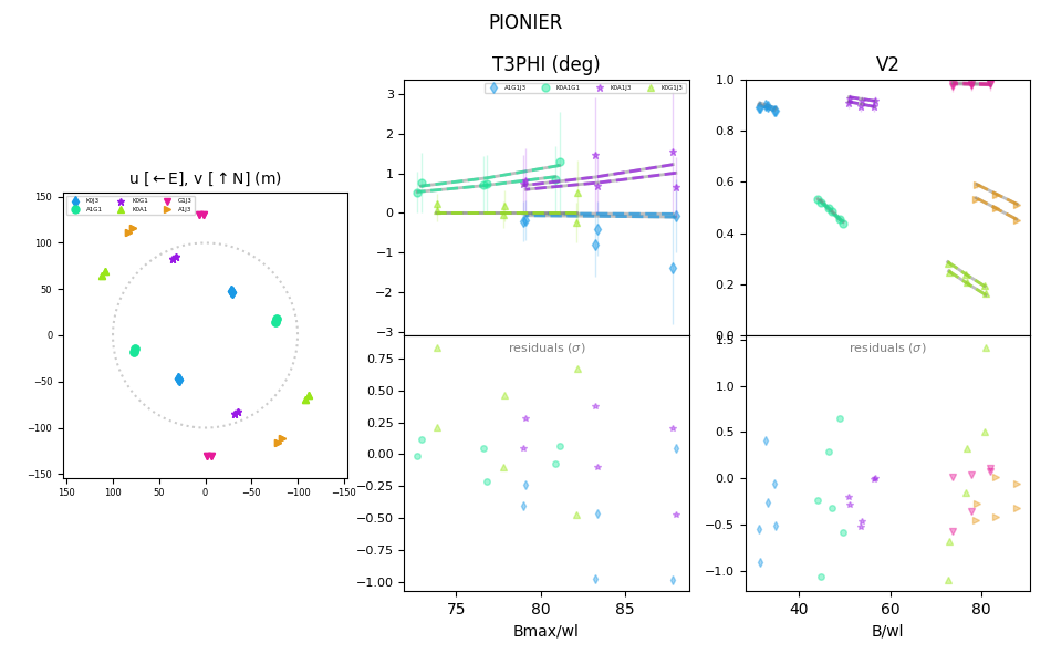
Figure 77: The best-fit data for HD 140008. On the left, the $u-v$ coverage from the observations with PIONIER can be seen. The different colours correspond to the telescope pair with which that particular data was acquired at the VLTI. In the middle, the closure phase (T3PHI) fit and residuals are shown in terms of the spatial frequency (B_avg/$\lambda$, written as Bavg/wl on the axes). On the right, the fit to the squared visibilities (V2) and the associated residuals are shown, again in terms of spatial frequency. Across the two fits, the data are represented as points whilst the fit as a continuous line.

Figure 78: Model image created based on the best-fitting model of HD 140008.

Figure 79: Plot showing the grid search used to search for the companion around HD 140008 and the companion’s significance.

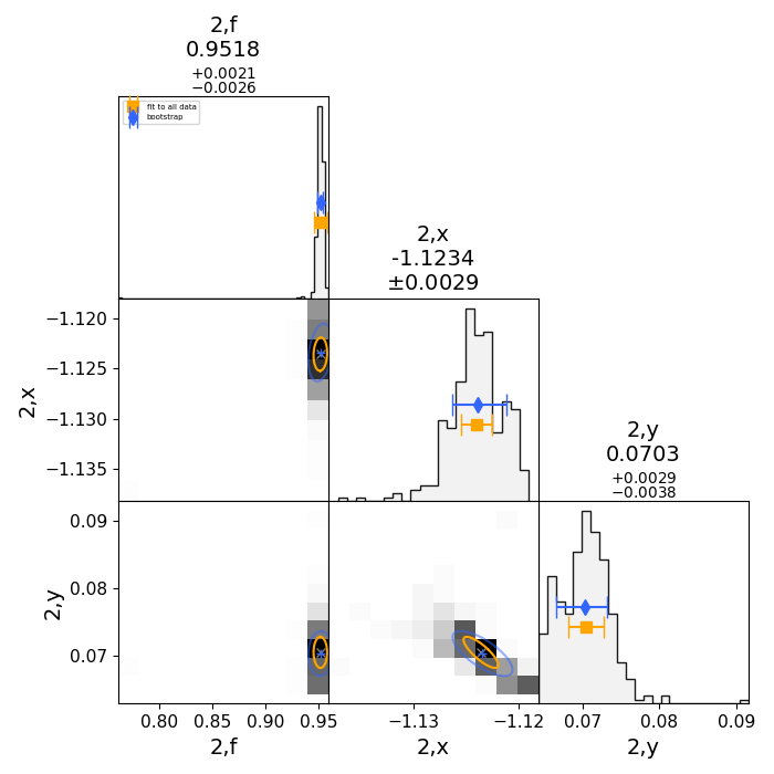
Figure 80: Bootstrapping plot showing the error determination for the dataset of HD 140008.

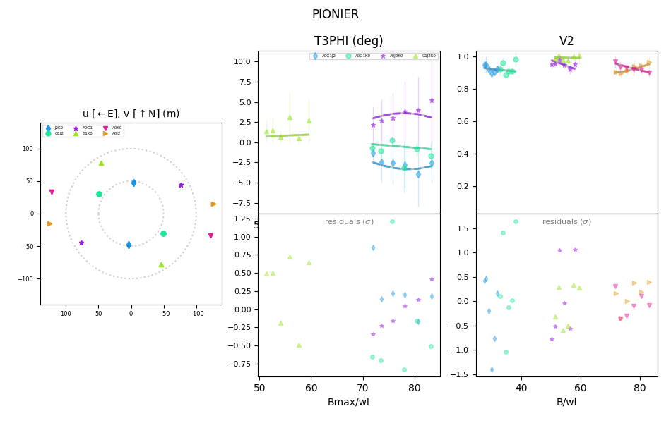
Figure 81: The best-fit data for HD 178175. On the left, the $u-v$ coverage from the observations with PIONIER can be seen. The different colours correspond to the telescope pair with which that particular data was acquired at the VLTI. In the middle, the closure phase (T3PHI) fit and residuals are shown in terms of the spatial frequency (B_avg/$\lambda$, written as Bavg/wl on the axes). On the right, the fit to the squared visibilities (V2) and the associated residuals are shown, again in terms of spatial frequency. Across the two fits, the data are represented as points whilst the fit as a continuous line.

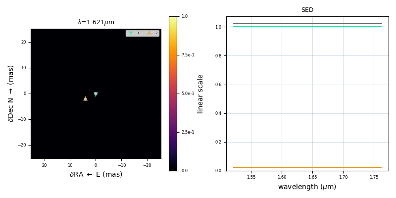
Figure 82: Model image created based on the best-fitting model of HD 178175.

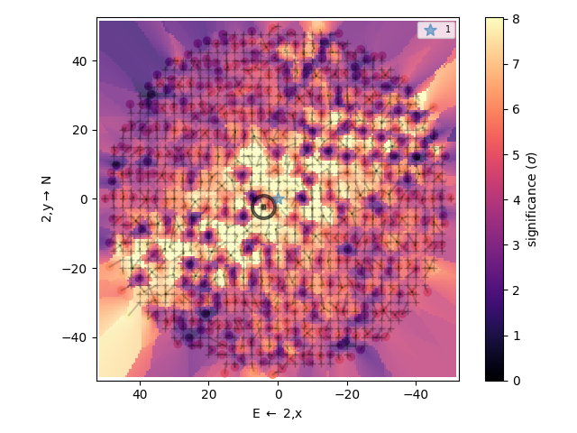
Figure 83: Plot showing the grid search used to search for the companion around HD 178175 and the companion’s significance.

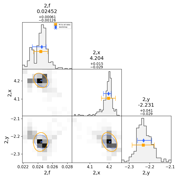
Figure 84: Bootstrapping plot showing the error determination for the dataset of HD 178175.

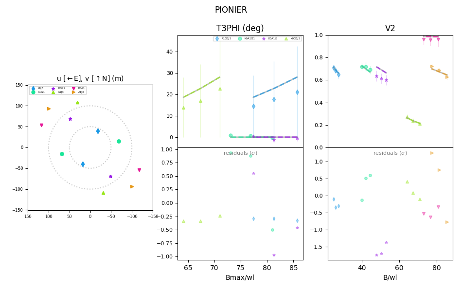
Figure 85: The best-fit data for HD 191263. On the left, the $u-v$ coverage from the observations with PIONIER can be seen. The different colours correspond to the telescope pair with which that particular data was acquired at the VLTI. In the middle, the closure phase (T3PHI) fit and residuals are shown in terms of the spatial frequency (B_avg/$\lambda$, written as Bavg/wl on the axes). On the right, the fit to the squared visibilities (V2) and the associated residuals are shown, again in terms of spatial frequency. Across the two fits, the data are represented as points whilst the fit as a continuous line.

Figure 86: Model image created based on the best-fitting model of HD 191263.

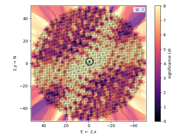
Figure 87: Plot showing the grid search used to search for the companion around HD 191263 and the companion’s significance.

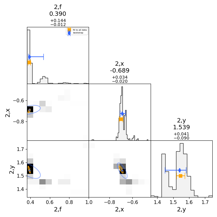
Figure 88: Bootstrapping plot showing the error determination for the dataset of HD 191263.

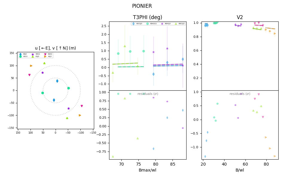
Figure 89: The best-fit data for HD 212076. On the left, the $u-v$ coverage from the observations with PIONIER can be seen. The different colours correspond to the telescope pair with which that particular data was acquired at the VLTI. In the middle, the closure phase (T3PHI) fit and residuals are shown in terms of the spatial frequency (B_avg/$\lambda$, written as Bavg/wl on the axes). On the right, the fit to the squared visibilities (V2) and the associated residuals are shown, again in terms of spatial frequency. Across the two fits, the data are represented as points whilst the fit as a continuous line.

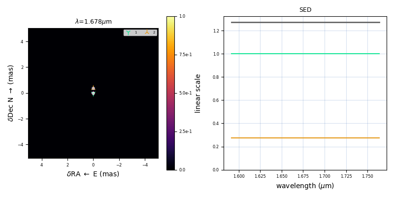
Figure 90: Model image created based on the best-fitting model of HD 212076.

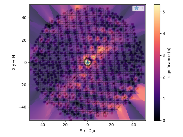
Figure 91: Plot showing the grid search used to search for the companion around HD 212076 and the companion’s significance.

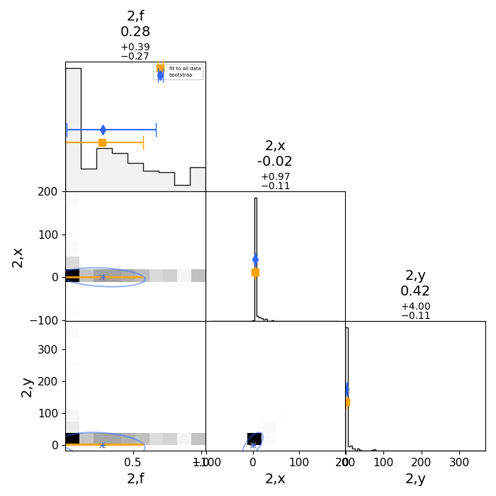
Figure 92: Bootstrapping plot showing the error determination for the dataset of HD 212076.

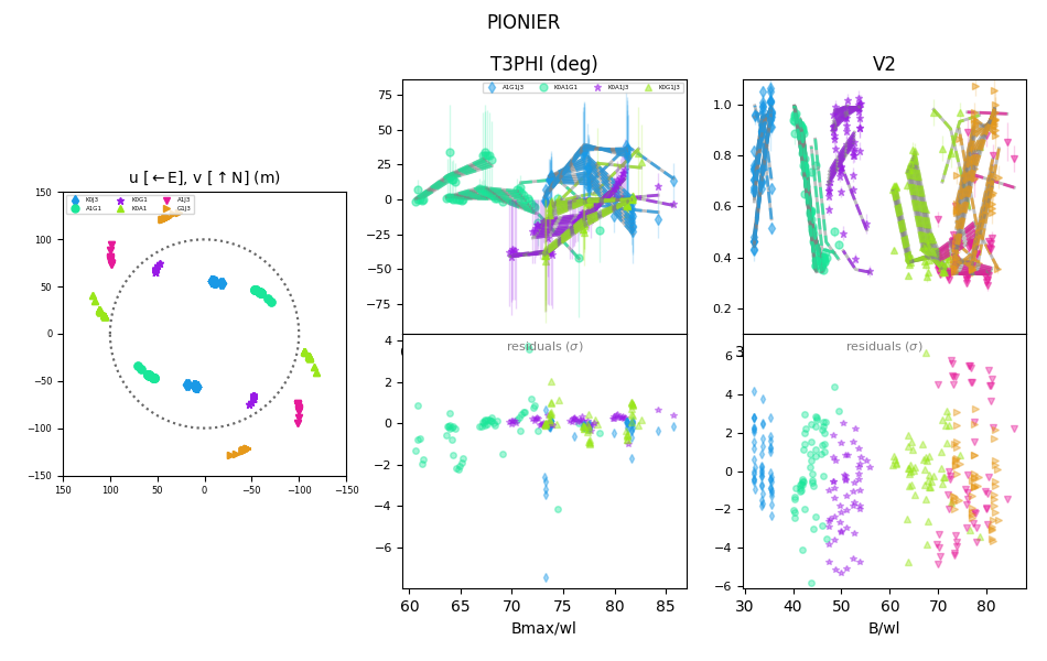
Figure 93: The best-fit data for HD 224990. On the left, the $u-v$ coverage from the observations with PIONIER can be seen. The different colours correspond to the telescope pair with which that particular data was acquired at the VLTI. In the middle, the closure phase (T3PHI) fit and residuals are shown in terms of the spatial frequency (B_avg/$\lambda$, written as Bavg/wl on the axes). On the right, the fit to the squared visibilities (V2) and the associated residuals are shown, again in terms of spatial frequency. Across the two fits, the data are represented as points whilst the fit as a continuous line.

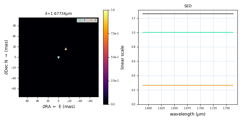
Figure 94: Model image created based on the best-fitting model of HD 224990.

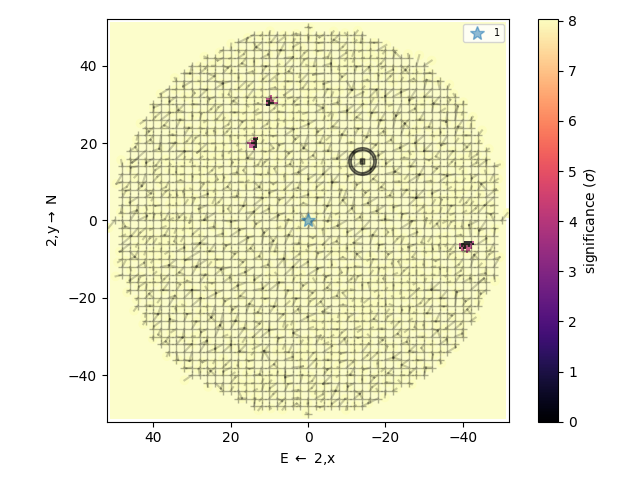
Figure 95: Plot showing the grid search used to search for the companion around HD 224990 and the companion’s significance.

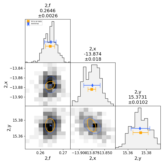
Figure 96: Bootstrapping plot showing the error determination for the dataset of HD 224990.

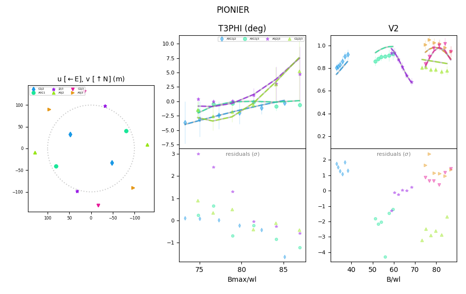
Figure 97: The best-fit data for HD 224990. On the left, the $u-v$ coverage from the observations with PIONIER can be seen. The different colours correspond to the telescope pair with which that particular data was acquired at the VLTI. In the middle, the closure phase (T3PHI) fit and residuals are shown in terms of the spatial frequency (B_avg/$\lambda$, written as Bavg/wl on the axes). On the right, the fit to the squared visibilities (V2) and the associated residuals are shown, again in terms of spatial frequency. Across the two fits, the data are represented as points whilst the fit as a continuous line.

Figure 98: Model image created based on the best-fitting model of HD 224990.

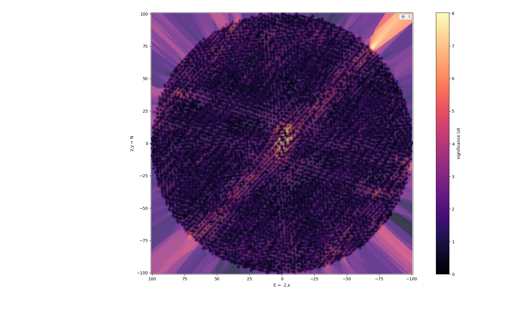
Figure 99: Plot showing the grid search used to search for the companion around HD 224990 and the companion’s significance.

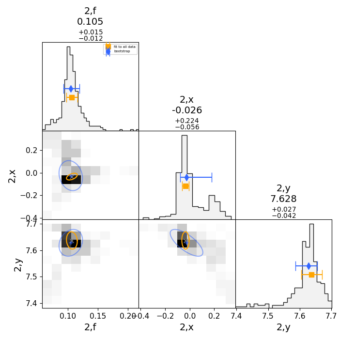
Figure 100: Bootstrapping plot showing the error determination for the dataset of HD 224990.

Figure 101: The best-fit data for HD 116658. On the left, the $u-v$ coverage from the observations with PIONIER can be seen. The different colours correspond to the telescope pair with which that particular data was acquired at the VLTI. In the middle, the closure phase (T3PHI) fit and residuals are shown in terms of the spatial frequency (B_avg/$\lambda$, written as Bavg/wl on the axes). On the right, the fit to the squared visibilities (V2) and the associated residuals are shown, again in terms of spatial frequency. Across the two fits, the data are represented as points whilst the fit as a continuous line.

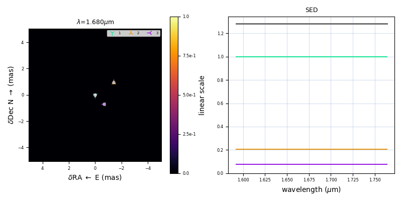
Figure 102: Model image created based on the best-fitting model of HD 116658.

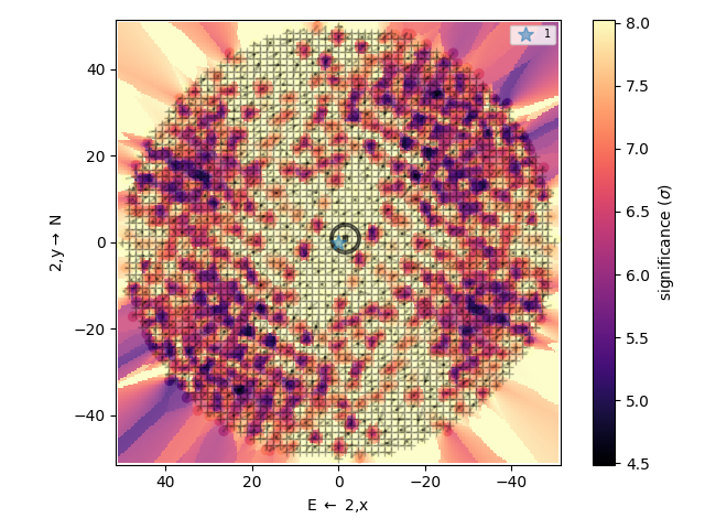
Figure 103: Plot showing the grid search used to search for the secondary companion around HD 116658 and the companion’s significance.

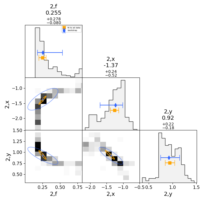
Figure 104: Bootstrapping plot showing the error determination for the parameters of the secondary star of HD 116658.

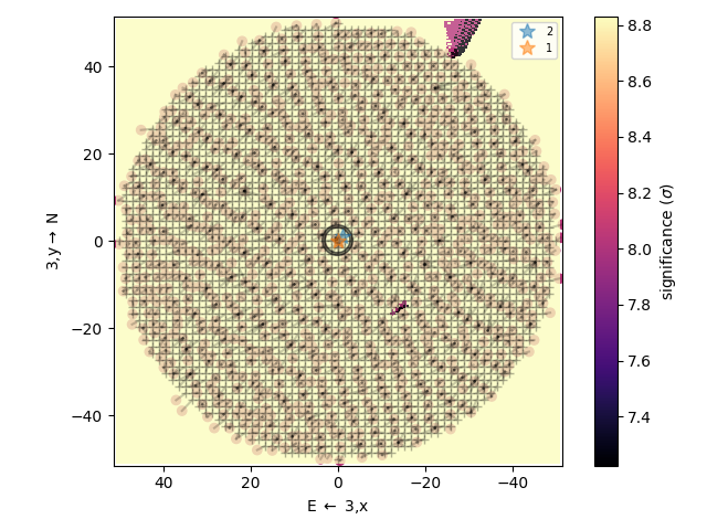
Figure 105: Plot showing the grid search used to search for the tertiary companion around HD 116658 and the companion’s significance.

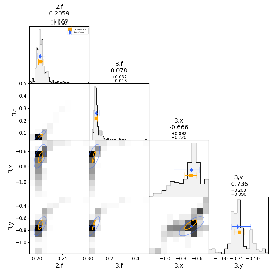
Figure 106: Bootstrapping plot showing the error determination of the tertiary star of HD 116658.

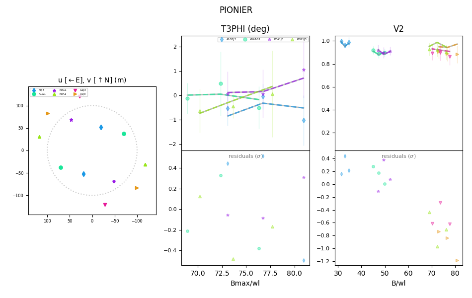
Figure 107: The best-fit data for HD 132058. On the left, the $u-v$ coverage from the observations with PIONIER can be seen. The different colours correspond to the telescope pair with which that particular data was acquired at the VLTI. In the middle, the closure phase (T3PHI) fit and residuals are shown in terms of the spatial frequency (B_avg/$\lambda$, written as Bavg/wl on the axes). On the right, the fit to the squared visibilities (V2) and the associated residuals are shown, again in terms of spatial frequency. Across the two fits, the data are represented as points whilst the fit as a continuous line.

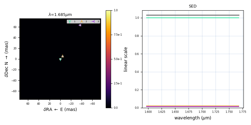
Figure 108: Model image created based on the best-fitting model of HD 132058.

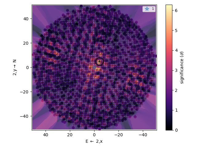
Figure 109: Plot showing the grid search used to search for the secondary companion around HD 132058 and the companion’s significance.

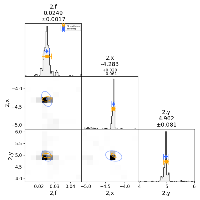
Figure 110: Bootstrapping plot showing the error determination for the parameters of the secondary star of HD 132058.

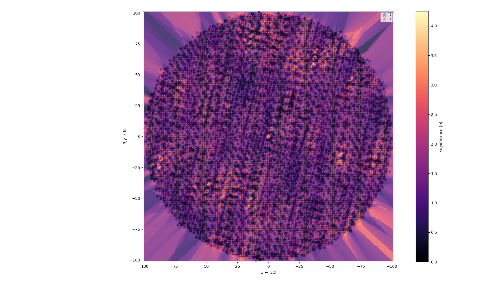
Figure 111: Plot showing the grid search used to search for the companion around HD 132058 and the companion’s significance.

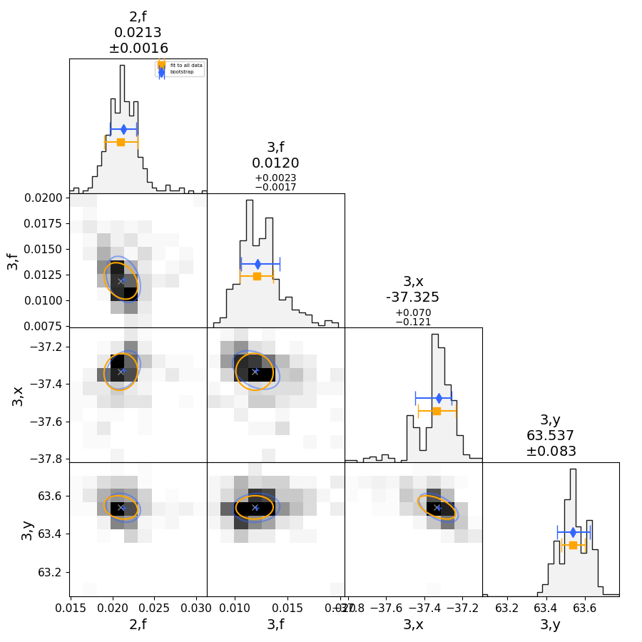
Figure 112: Bootstrapping plot showing the error determination for the dataset of HD 132058.

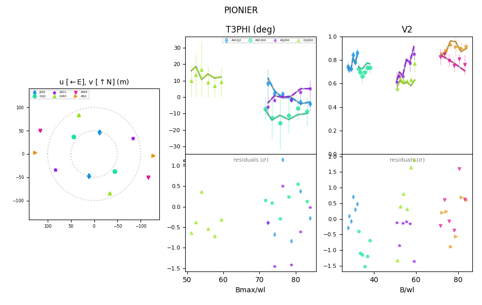
Figure 113: The best-fit data for HD 147932. On the left, the $u-v$ coverage from the observations with PIONIER can be seen. The different colours correspond to the telescope pair with which that particular data was acquired at the VLTI. In the middle, the closure phase (T3PHI) fit and residuals are shown in terms of the spatial frequency (B_avg/$\lambda$, written as Bavg/wl on the axes). On the right, the fit to the squared visibilities (V2) and the associated residuals are shown, again in terms of spatial frequency. Across the two fits, the data are represented as points whilst the fit as a continuous line.

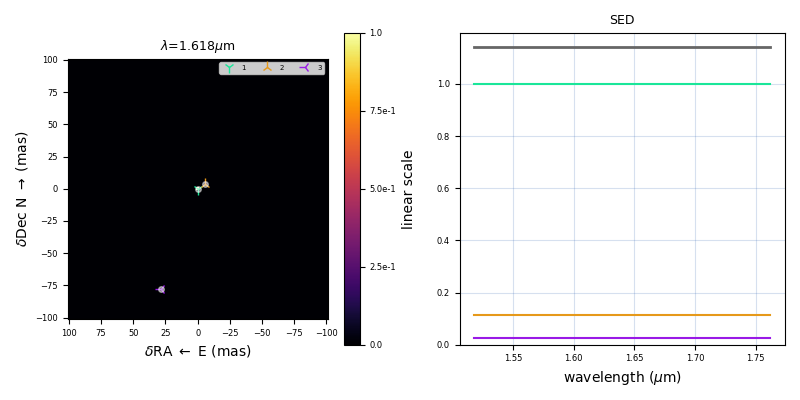
Figure 114: Model image created based on the best-fitting model of HD 147932.

Figure 115: Plot showing the grid search used to search for the secondary companion around HD 147932 and the companion’s significance.

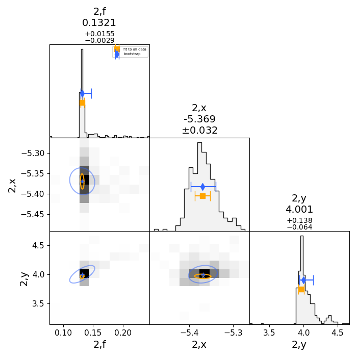
Figure 116: Bootstrapping plot showing the error determination for the parameters of the secondary star of HD 147932.

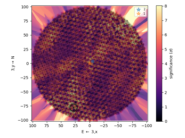
Figure 117: Plot showing the grid search used to search for the tertiary companion around HD 147932 and the companion’s significance.

Figure 118: Bootstrapping plot showing the error determination for tertiary of HD 147932.

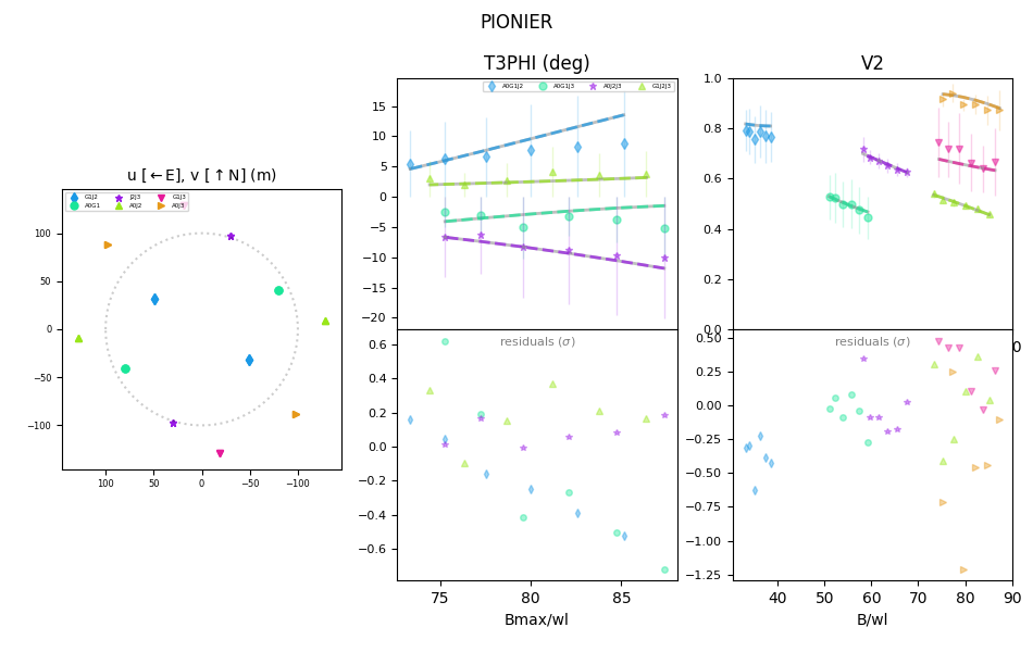
Figure 119: The best-fit data for HD 161701. On the left, the $u-v$ coverage from the observations with PIONIER can be seen. The different colours correspond to the telescope pair with which that particular data was acquired at the VLTI. In the middle, the closure phase (T3PHI) fit and residuals are shown in terms of the spatial frequency (B_avg/$\lambda$, written as Bavg/wl on the axes). On the right, the fit to the squared visibilities (V2) and the associated residuals are shown, again in terms of spatial frequency. Across the two fits, the data are represented as points whilst the fit as a continuous line.

Figure 120: Model image created based on the best-fitting model of HD 161701.

Figure 121: Plot showing the grid search used to search for the secondary companion around HD 161701 and the companion’s significance.

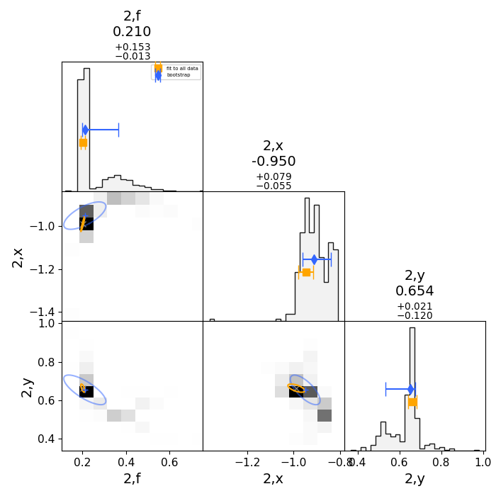
Figure 122: Bootstrapping plot showing the error determination for the parameters of the secondary star of HD 161701.

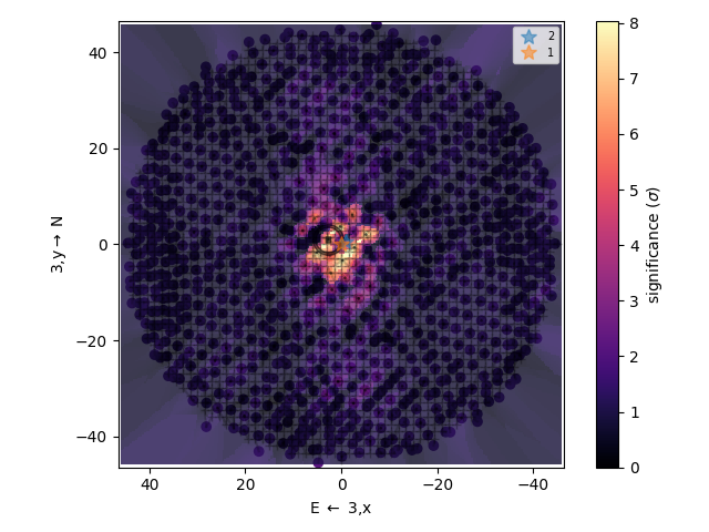
Figure 123: Plot showing the grid search used to search for the tertiary companion around HD 161701 and the companion’s significance.

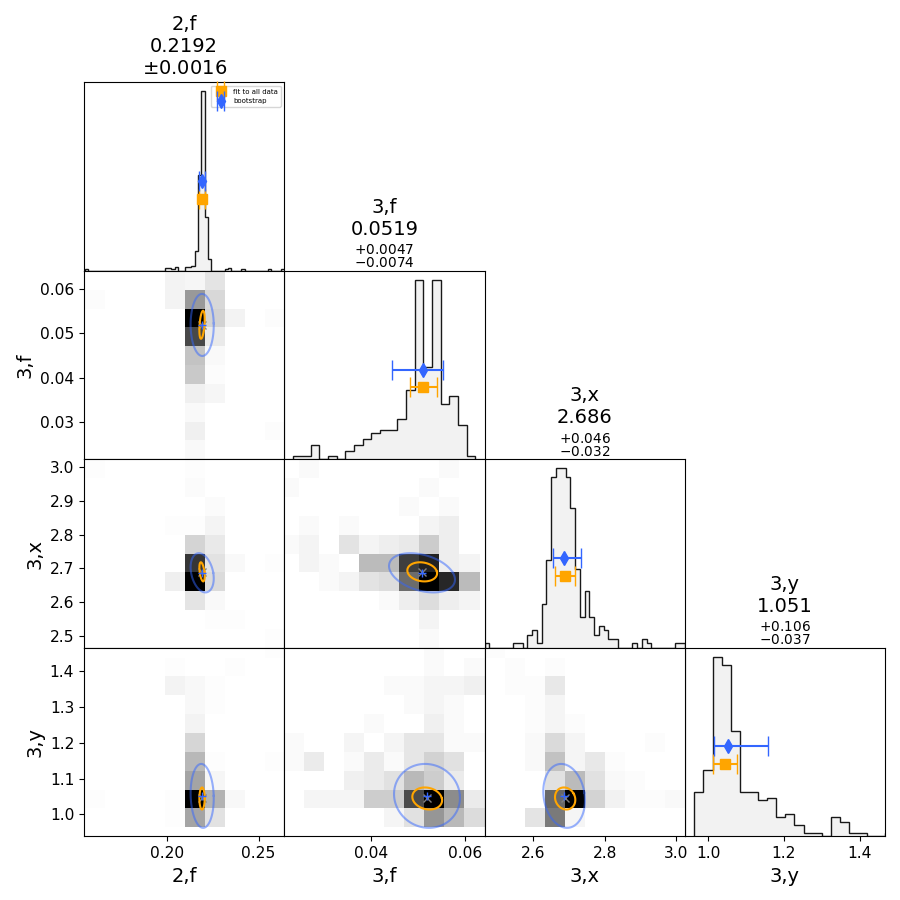
Figure 124: Bootstrapping plot showing the error determination for the tertiary HD 161701.

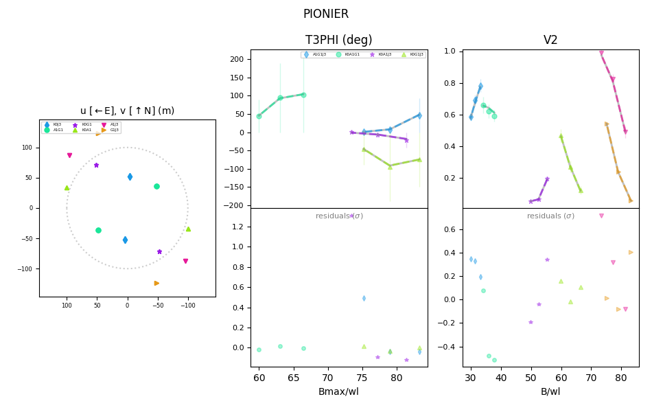
Figure 125: The best-fit data for HD 193933. On the left, the $u-v$ coverage from the observations with PIONIER can be seen. The different colours correspond to the telescope pair with which that particular data was acquired at the VLTI. In the middle, the closure phase (T3PHI) fit and residuals are shown in terms of the spatial frequency (B_avg/$\lambda$, written as Bavg/wl on the axes). On the right, the fit to the squared visibilities (V2) and the associated residuals are shown, again in terms of spatial frequency. Across the two fits, the data are represented as points whilst the fit as a continuous line.

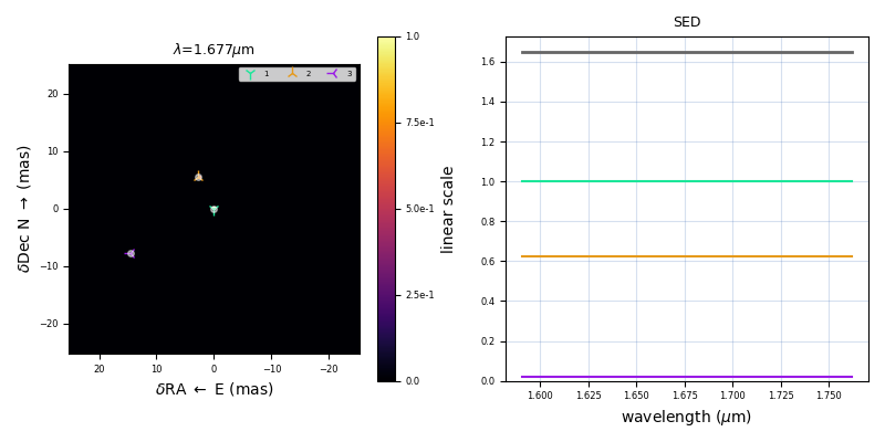
Figure 126: Model image created based on the best-fitting model of HD 193933.

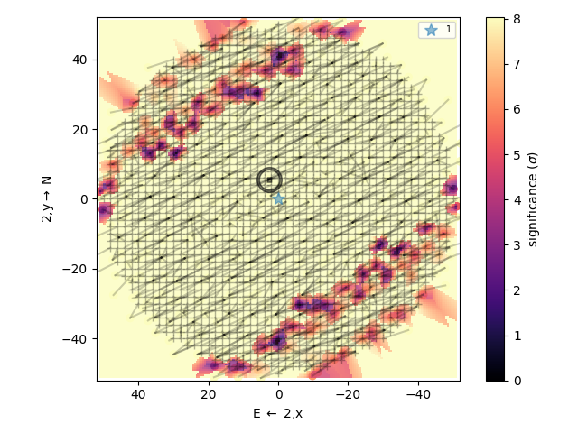
Figure 127: Plot showing the grid search used to search for the secondary companion around HD 193933 and the companion’s significance.

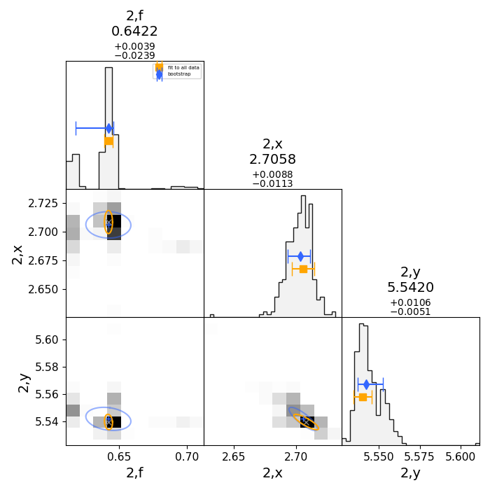
Figure 128: Bootstrapping plot showing the error determination for the parameters of the secondary star of HD 193933.

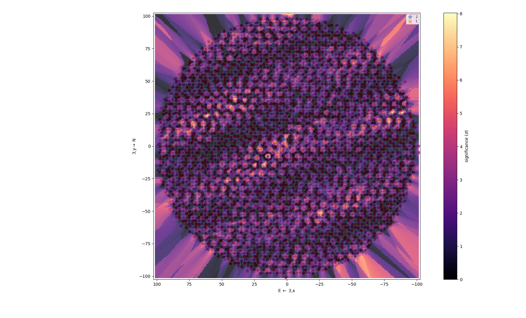
Figure 129: Plot showing the grid search used to search for the tertiary companion around HD 193933 and the companion’s significance.

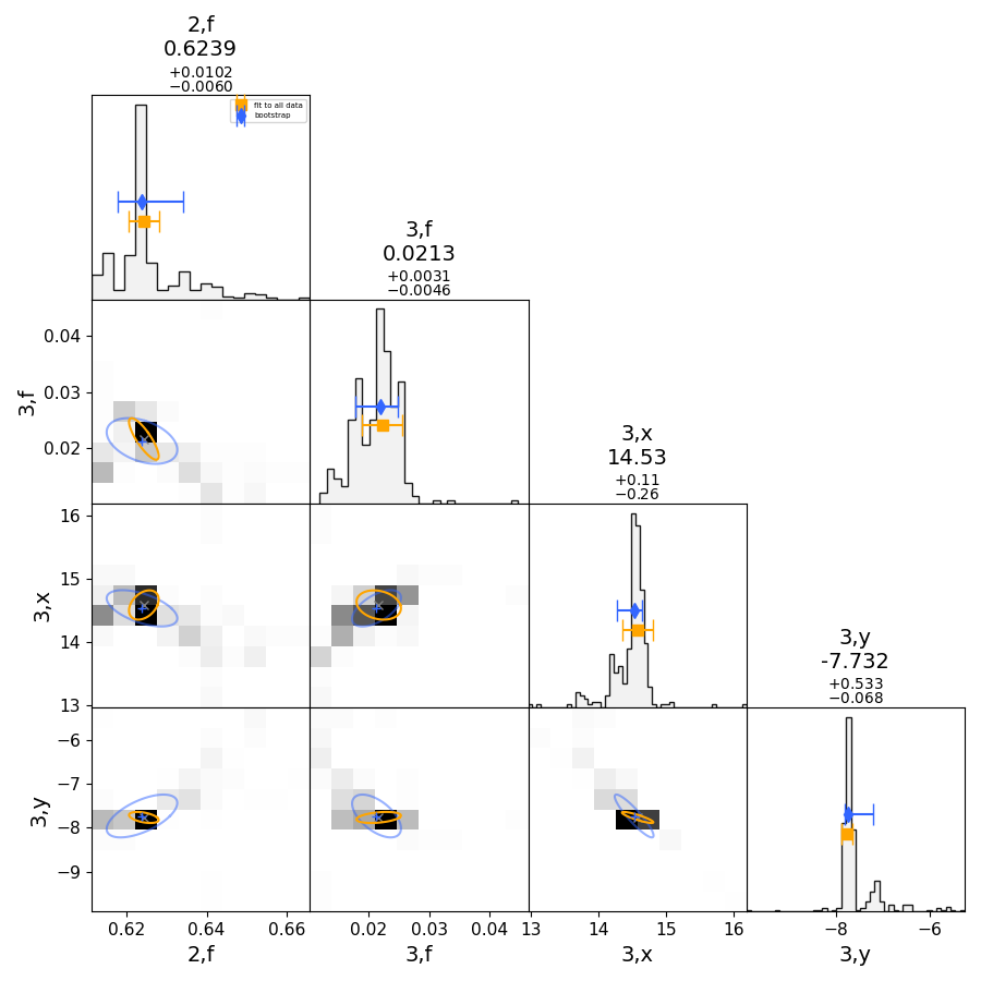
Figure 130: Bootstrapping plot showing the error determination for the tertiary of HD 193933.