Adaptive Scoring and Thresholding with Human Feedback for Robust Out-of-Distribution Detection

Abstract

Machine Learning (ML) models are trained on in-distribution (ID) data but often encounter out-of-distribution (OOD) inputs during deployment—posing serious risks in safety-critical domains. Recent works have focused on designing scoring functions to quantify OOD uncertainty, with score thresholds typically set based solely on ID data to achieve a target true positive rate (TPR), since OOD data is limited before deployment. However, these TPR-based thresholds leave false positive rates (FPR) uncontrolled, often resulting in high FPRs where OOD points are misclassified as ID. Moreover, fixed scoring functions and thresholds lack the adaptivity needed to handle newly observed, evolving OOD inputs, leading to sub-optimal performance. To address these challenges, we propose a human-in-the-loop framework that safely updates both scoring functions and thresholds on the fly based on real-world OOD inputs. Our method maximizes TPR while strictly controlling FPR at all times, even as the system adapts over time. We provide theoretical guarantees for FPR control under stationary conditions and present extensive empirical evaluations on OpenOOD benchmarks to demonstrate that our approach outperforms existing methods by achieving higher TPRs while maintaining FPR control.

1 Introduction

Machine learning (ML) models are typically trained under the closed-world assumption—test-time data comes from the same distribution as the training data (in-distribution, or ID). However, during deployment, models often encounter out-of-distribution (OOD) inputs, such as data points that do not belong to any training class in classification. In safety-critical domains like medical diagnosis, it is crucial that the system refrains from generating predictions for OOD inputs. Instead, these inputs must be flagged so that corrective actions can be taken or human intervention sought. To achieve this, an OOD detector is integrated into systems to monitor real-time samples and flag those that appear OOD, ensuring that unreliable predictions are not produced.

To this end, many OOD detection methods have been developed to distinguish OOD inputs from ID inputs (Yang et al., 2022). While ID data is available during model training, diverse OOD examples remain unseen until deployment. This limited access to OOD data naturally leads to an ID-based detection approach: (1) a scoring function is designed or selected to quantify how likely an input is to be OOD (or ID) using only ID data, and (2) a threshold is set on these scores—again based solely on ID data—to achieve a desired true positive rate (TPR) (e.g., 95% of ID inputs are correctly identified as ID). While this approach has shown promising results, it suffers from the following issues:

1) High False Positive Rate (FPR). OOD detection systems are prone to false positives, where OOD inputs are misclassified as ID (Nguyen et al., 2015; Amodei et al., 2016). In high-risk applications, false positives are often more critical than false negatives. For example, detecting non-existent cancer may simply trigger further analysis, whereas missing an actual case can be fatal. Thus, systems in such domains must have strict FPR control (e.g., below 5%). However, the common approach sets score thresholds solely using ID data to meet a target TPR, leaving FPR uncontrolled. As a result, FPRs can be very high—for instance, ranging from 32% to 91% when CIFAR-10 is used as ID in the OpenOOD benchmark (Yang et al., 2022).

2) Lack of Adaptivity. During deployment, systems encounter diverse, unseen OOD inputs. However, no single scoring function works universally well for all types of OOD data. As a result, the common approach of relying on a pre-designed scoring function and threshold risks being stuck with one that performs poorly on newly encountered OOD inputs—thereby limiting achievable TPR. These methods miss the opportunity to improve their scoring functions based on OOD inputs observed during deployment (Figure 3). In light of these limitations, real-world systems must adapt their scoring functions and thresholds over time to handle diverse OOD inputs, maximizing TPR while keeping FPR under control.

These challenges—high FPR and lack of adaptivity—motivate the following goal.

Toward this goal, we make the following contributions:

1. We introduce a framework that leverages human feedback to identify OOD inputs and simultaneously update scoring functions and thresholds, thereby maximizing TPR while ensuring strict FPR control throughout deployment (Figure 1).

2. We provide a theoretical analysis that guarantees FPR control at all times, even as scoring functions and thresholds are updated. Our analysis shows that our approach can maintain FPR below a user-specified tolerance $\alpha$ (e.g., 5%) when the OOD remains constant.

3. We present extensive empirical evaluations under two different conditions: when the OOD remains the same (stationary) and when it changes over time (nonstationary). By comparing our method to baselines on OpenOOD benchmarks, we demonstrate that our framework consistently outperforms existing approaches, achieving higher TPR while ensuring strict FPR control.

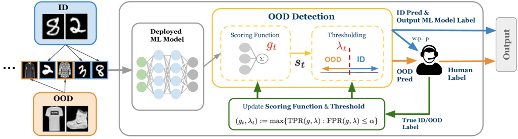
Figure 1: Overview of the ASAT workflow, updating both scoring function $g_{t}$ and thresholds $\lambda_{t}$ via human feedbacks.

We refer to our method as ASAT (adaptive scoring, adaptive threshold) in contrast to the common approach, denoted as FSFT (fixed scoring, fixed threshold), which uses fixed scoring functions and thresholds derived from ID data. We also compare with FSAT (fixed scoring, adaptive threshold), which updates thresholds while keeping scoring functions fixed. Please refer to Section 3.3 for descriptions of FSAT. See Table 2 for a high-level summary and comparison.

Method	Score Fn	Threshold	FPR $\bm{\leq\alpha}$	TPR
FSFT	Fixed	Fixed	$\times$	Fixed (95%)
FSAT	Fixed	Adaptive	$\checkmark$	Limited
ASAT	Adaptive	Adaptive	$\checkmark$	Improved

Figure 2: Comparison of scoring functions, thresholds, FPR control, and TPR for FSFT, FSAT, and ASAT.

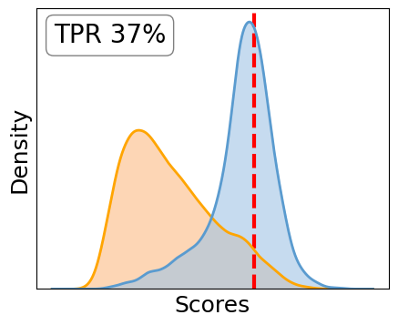
(a) EBO

(b) KNN

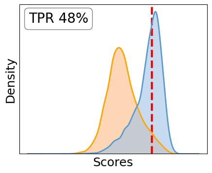
(c) VIM

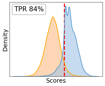
(d) Optimal $g^{\ast}$ from (P1)

Figure 3: Comparison of score distributions between post-hoc fixed scoring functions (trained solely on ID data) and our learned function $g^{\ast}$ (trained offline on both ID and OOD). CIFAR-10 and Places365 are the ID and OOD datasets, respectively. As $t$ increases, the ASAT-adapted scoring functions converge toward $g^{\ast}$, which achieves the highest TPR at 5% FPR compared to EBO, KNN, and VIM methods from the Open-OOD benchmarks. This comparison suggests that incorporating human-labeled OOD inputs encountered during deployment enables ASAT to update scoring functions that better align with real-world OOD points. For more details, see Section 5.

2 Preliminaries

2.1 Problem Setting

Data Stream. Let $\mathcal{X}\subseteq\mathbb{R}^{d}$ and $\mathcal{Y}=\{0,1\}$ denote feature and label spaces, respectively, where 0 represents OOD and 1 represents ID. Let $\mathcal{D}_{0}$ and $\mathcal{D}_{1}$ be the unknown distributions of the OOD and ID data over $\mathcal{X}$. At each time $t$ during deployment, our model sequentially receives a sample $x_{t}$ drawn independently from the mixture model,

$$x_{t}\overset{\mathrm{i.i.d.}}{\sim}\gamma\mathcal{D}_{0}+(1-\gamma)\mathcal{D}_{1},$$

where the mixture rate $\gamma\in(0,1)$ is fixed but unknown. Let $y_{t}\in\mathcal{Y}$ be the true label for $x_{t}$, indicating whether it is an OOD or ID point.

Scoring Functions. Let $\mathcal{G}\subset\{g:\mathcal{X}\rightarrow\mathcal{S}\subseteq\mathbb{R}\}$ denote a class of scoring functions. For each $x_{t}$, a scoring function $g\in\mathcal{G}$ computes the score $s_{t}:=g(x_{t})\in\mathcal{S}$. We assume that higher scores correspond to a higher likelihood of $x_{t}$ being ID. Then, the OOD classifier is defined by the threshold function $h_{\lambda}:\mathcal{S}\rightarrow\mathcal{Y}$ as

$$h_{\lambda}(s_{t})\vcentcolon=\mathbbm{1}\{s_{t}>\lambda\},$$

with $\lambda\in\Lambda$. The prediction label is $\widehat{y}_{t}:=h_{\lambda}(s_{t})$. The parameter $\lambda$ defines the threshold for classifying $x_{t}$ as either OOD or ID. Thus, setting $\lambda$ carefully is crucial to ensure safety in OOD detection. In FSFT, both $g$ and $\lambda$ remain fixed for all $t\geq 1$. In contrast, ASAT aims to update both $g_{t}$ and $\lambda_{t}$ using incoming OOD inputs, thereby better controlling FPR and maximizing TPR.

Population-level FPR and TPR. Given any $g\in\mathcal{G}$ and $\lambda\in\Lambda$, the true FPR and TPR for scores are defined as

$$\text{FPR}(g,\lambda) =\mathbb{E}_{x\sim\mathcal{D}_{0}}[\mathbbm{1}\{g(x)>\lambda\}],$$ (1)

$$\text{TPR}(g,\lambda) =\mathbb{E}_{x\sim\mathcal{D}_{1}}[\mathbbm{1}\{g(x)>\lambda\}].$$

Given $g$, FPR and TPR are monotonically decreasing in $\lambda$ (Figure 4).

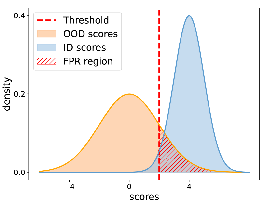
Figure 4: An example of OOD and ID score distributions mapped by $g$ with a decision threshold $\lambda$. The hatched region is the FPR density.

3 Methodology

We propose ASAT (Figure 1) that adaptively updates both scoring functions and thresholds based on human-labeled OOD samples observed during deployment. This adaptation is crucial, as the initial scoring function and threshold—typically developed solely on ID data—may lead to high FPR or suboptimal performance on certain OOD cases.

3.1 ASAT Workflow

At each time $t$, the system processes an input $x_{t}$ using scoring function $\widehat{g}_{t-1}$ and threshold $\widehat{\lambda}_{t-1}$, both learned at the previous time $t-1$ (see Section 3.2 for the learning process). It first computes score $s_{t}=\widehat{g}_{t-1}(x_{t})$ for $x_{t}$. If $s_{t}<\widehat{\lambda}_{t-1}$, then $x_{t}$ is considered OOD and receives a human label $y_{t}\in\{0,1\}$. If $s_{t}\geq\widehat{\lambda}_{t-1}$, $x_{t}$ is considered ID, and in this case, we obtain the human label $y_{t}$ only with probability $p\in(0,1)$. We refer to this selective sampling as importance sampling. This importance sampling enables the detection of OOD shifts and allows for unbiased FPR estimation, which is essential to maintain FPR control.

3.2 Learning Scoring Functions and Thresholds

In this section, we describe how ASAT learns scoring functions and thresholds at each time $t$. We first define the optimal scoring function and threshold based on the TPR and FPR (1), which are unknown in practice. We then present a tractable and practical learning method only using finite samples and estimates.

Optimal Scoring Function and Threshold. ASAT aims to maintain strict FPR control during deployment while minimizing human intervention. In practice, accurately predicting IDs reduces the need for human verification. Hence, maximizing TPR effectively minimizes human intervention. With this, we formulate the ASAT objective as a joint optimization problem to find the optimal $(g^{\star},\lambda^{\star})$ that maximizes TPR under the constraint FPR $\leq\alpha$.

Here, $\alpha$ is the user-specified tolerance level for FPR (e.g., $\alpha=0.05$ implies FPR must be below 5% at all times). However, since $\mathcal{D}_{0}$ and $\mathcal{D}_{1}$ are unknown, the true values of TPR and FPR for a given $(g,\lambda)$ are not accessible, making (P1) intractable. Consequently, we must estimate FPR and TPR based on the finite samples collected by time $t$.

FPR and TPR Estimates. We assume that ID data is largely available, whereas diverse OOD data is not accessible before deployment. Thus, ASAT identifies real-world OOD points via human feedback (i.e., importance sampling), while relying on a fixed, i.i.d ID dataset from training. Let $X_{t}^{(ood)}$ denote the OOD samples collected up to time $t$ (see Section 3.1), and let $X_{0}^{(id)}$ be the fixed ID dataset. Then, for a given scoring function and threshold pair $(g,\lambda)$, the FPR estimate at time $t$ is defined as

$$\widehat{\text{FPR}}_{t}(g,\lambda)=\frac{\sum_{u=1}^{t}Z_{u}\cdot\mathbbm{1}\{g(x_{u})>\lambda\}}{\sum_{u=1}^{t}Z_{u}},$$ (2)

where

$$Z_{u}:=\begin{cases}1&\text{if }s_{u}<\widehat{\lambda}_{u-1},i_{u}=0,y_{u}=0,\\ \frac{1}{p}&\text{if }s_{u}\geq\widehat{\lambda}_{u-1},i_{u}=1,y_{u}=0,\\ 0&\text{otherwise},\end{cases}$$

and $i_{u}$ indicate whether $x_{u}$ was importance sampled at time $u$. On the other hand, we estimate TPR using $X_{0}^{(id)}$ as

$$\widehat{\text{TPR}}(g,\lambda) =\frac{1}{|X_{0}^{(id)}|}\sum_{x\in X_{0}^{(id)}}\mathbbm{1}\{g(x)>\lambda\}.$$ (3)

Note for a fixed $g$ and $\lambda$ the $\widehat{\text{TPR}}(g,\lambda)$ is constant over time, since $X_{0}^{(id)}$ is fixed.

Relaxations of (P1). Using the TPR and FPR estimates from eq (2) and (3), we can formulate a tractable optimization problem for the ASAT objective. However, because the indicator sums are non-differentiable and difficult to optimize, we further approximate them using a sigmoid function defined as $\sigma(\kappa,z)\vcentcolon=1/(1+\exp{(-\kappa z)})$, $\kappa>0$, which satisfies $\lim\limits_{\kappa\rightarrow\infty}\sigma(\kappa,z)=\mathbbm{1}\{z>0\}.$ This yields the following smooth surrogate estimates of the TPR and FPR:

$$\widetilde{\text{FPR}}_{t}(g,\lambda)\vcentcolon=\frac{\sum_{u=1}^{t}Z_{u}\cdot\sigma(\kappa,g(x_{u})-\lambda)}{\sum_{u=1}^{t}Z_{u}},$$ (4)

$$\widetilde{\text{TPR}}(g,\lambda)\vcentcolon=\frac{1}{|X_{0}^{(id)}|}\sum_{x\in X_{0}^{(id)}}\sigma(\kappa,g(x)-\lambda).$$ (5)

The problem obtained by replacing the true FPR and TPR in (P1) with these surrogates is a non-convex constrained optimization problem. Although this type of problem has been widely studied (Park and Van Hentenryck, 2023; Jia and Grimmer, 2022), it remains challenging to solve efficiently in practice. Therefore, we reformulate it in a regularization form as follows.

The hyperparameter $\beta\geq 0$ controls the trade-off between maximizing TPR and minimizing FPR. This formulation enables efficient gradient-based optimization of $g$ and $\lambda$. With this, at each time $t$, ASAT estimates TPR and FPR using (4) and (5), then it solves the problem (P2). However, some issues remain to be addressed.

Periodically Learning Scoring Functions. Solving (P2) at every time $t$ is computationally expensive, especially when only a few new OOD points have been identified. To address this, ASAT optimizes (P2) only periodically—when enough new OOD samples have been collected since the last update. Let $U_{t}$ denote the number of updates to $g$ performed by time $t$, and define $\omega^{ood}_{i}$ as the user-specified optimization frequency for $(i+1)$th update (e.g., $\omega^{ood}_{1}$ indicates the number of new OOD samples required for the second update). Define $\Delta^{ood}_{t}$ as the number of new OOD samples identified by time $t$ since the last update. At time $t$, ASAT updates its scoring function only if $\Delta^{ood}_{t}\geq\omega^{ood}_{U_{t}}$.

Model Selection. Assume an update occurs at time $t$ (i.e., $\Delta^{ood}_{t}\geq\omega^{ood}_{U_{t}}$) by solving (P2). However, the newly learned $\widehat{g}_{t}$ may underperform $\widehat{g}_{t-1}$ in terms of TPR at a given $\lambda$. To prevent this, we do a model selection by applying the TPR criterion:

$$\widehat{\text{TPR}}(\widehat{g}_{t},\widehat{\lambda}_{t})+2\zeta(\delta,|X_{0}^{(id)}|)>\widehat{\text{TPR}}(\widehat{g}_{t-1},\widehat{\lambda}_{t-1}).$$

Here, $\widehat{\lambda}_{t}$ is obtained from (Q1) (see Section 3.3), and $\zeta(\delta,|X_{0}^{(id)}|)$ is the Dvoretzky–Kiefer–Wolfowitz (DKW) confidence interval, valid w.p. at least $1-\delta$ (Nadaraya, 1965). If this is violated, we let $\widehat{g}_{t}=\widehat{g}_{t-1}$.

Threshold Estimation. The solution $(\widehat{g}_{t},\widehat{\lambda}_{t}^{\prime})$ obtained from (P2) may violate the FPR constraint in (P1), since (P2) is unconstrained. That is, it could yield $\text{FPR}(\widehat{g}_{t},\widehat{\lambda}_{t}^{\prime})>\alpha,$ which undermines our goal of keeping FPR below $\alpha$ at all times in ASAT. To strictly enforce the FPR constraint, we introduce a new step: we estimate a revised threshold $\widehat{\lambda}_{t}$ for $\widehat{g}_{t}$ using the threshold estimation method proposed by Vishwakarma et al. (2024c).

3.3 Learning Thresholds

To ensure that the FPR constraint is satisfied throughout the deployment, we leverage the threshold estimation method FSAT (fixed scoring, adaptive threshold). See Table 2 for the differences between FSFT, FSAT, and ASAT.

FSAT for Threshold Estimation. The high-level idea of FSAT is to find a safe threshold for a fixed scoring function at each time $t$ such that FPR (1) is below $\alpha$. Given $(\widehat{g}_{t},\widehat{\lambda}_{t}^{\prime})$ from (P2), we discard the potentially unsafe $\widehat{\lambda}_{t}^{\prime}$ and compute a safe threshold $\widehat{\lambda}_{t}$ via the FPR estimate from eq (2). We achieve this by constructing a uniformly valid upper confidence bound (UCB) on the error between the estimated and true FPR.

Upper Confidence Bound (UCB). At each time $t$, the UCB is constructed as

$$\psi_{t}(\delta):=\sqrt{\frac{3c_{t}}{N_{t}^{(o)}}\left[2\log\log\left(\frac{3c_{t}N_{t}^{(o)}}{2}\right)+2\log\left(\frac{4U_{t}|\Lambda|}{\delta}\right)\right]},$$ (6)

where $\delta\in(0,1)$ is the failure probability, and $c_{t}$ is a time-dependent variable. Intuitively, the UCB guarantees that w.p. at least $1-\delta$,

$$\widehat{\text{FPR}}_{t}(\widehat{g}_{t},\lambda)\in\Big{[}\text{FPR}(\widehat{g}_{t},\lambda)-\psi_{t}(\delta),\text{FPR}(\widehat{g}_{t},\lambda)+\psi_{t}(\delta)\Big{]},$$

for all times $t\geq 1$ and thresholds $\lambda\in\Lambda$. That is, with high probability, the FPR estimate (2) is within $\psi_{t}(\delta)$ of the true FPR. In Section 4, we provide further details, formal statements, and demonstrate that the UCB is valid for time-varying scoring functions. This leads to the optimization problem for adapting thresholds for a given $\widehat{g}_{t}$ in ASAT as

The problem (Q1) can be directly solved via binary search. Since TPR is monotonically decreasing in $\lambda$ and $\widehat{g}_{t}$ is fixed, we reduce the objective from maximizing TPR to minimizing $\lambda$. Consequently, the solution $\widehat{\lambda}_{t}$ from (Q1), together with $\widehat{g}_{t}$, satisfies the FPR constraint with high probability, i.e., $\text{FPR}(\widehat{g}_{t},\widehat{\lambda}_{t})\leq\alpha$ (see Proposition 1 for more details).

Below is an overview of ASAT. See Appendix B for further details and complete algorithms.

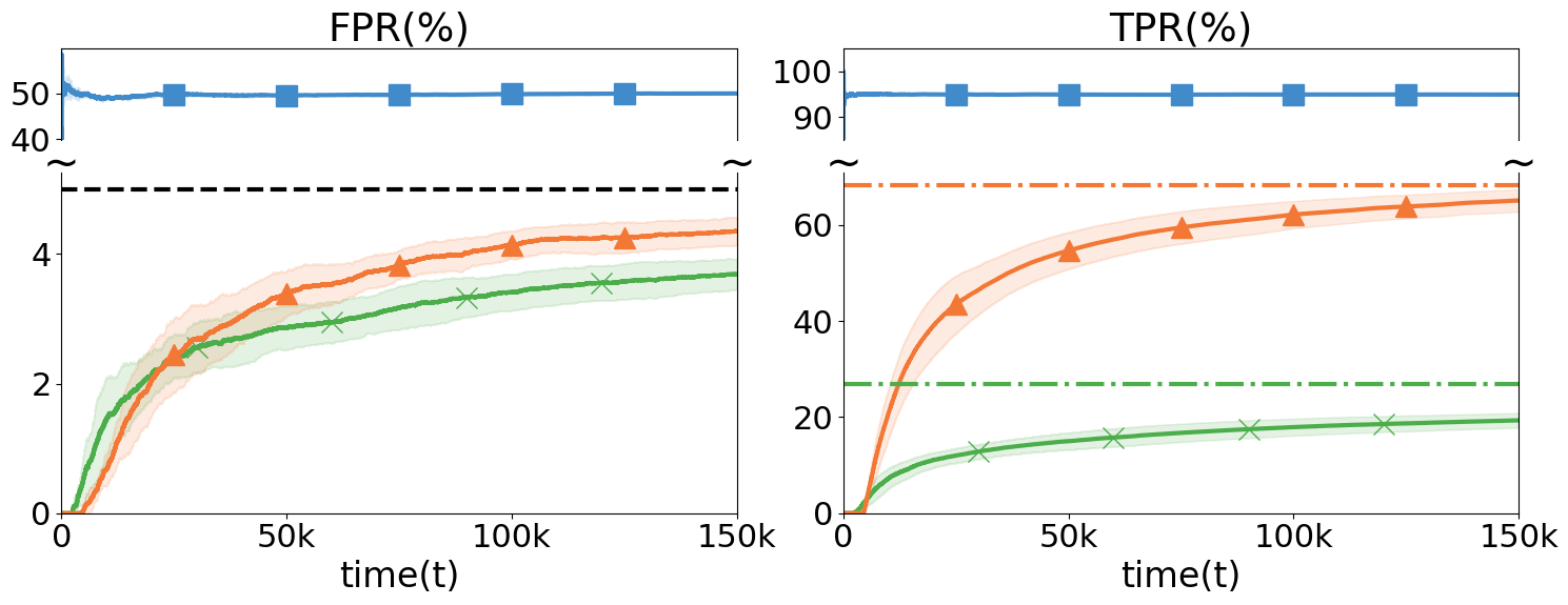
(a) Stationary, EBO, CIFAR-100 as OOD.

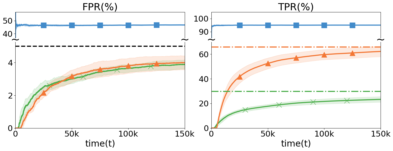
(b) Stationary, EBO, Near-OOD as OOD.

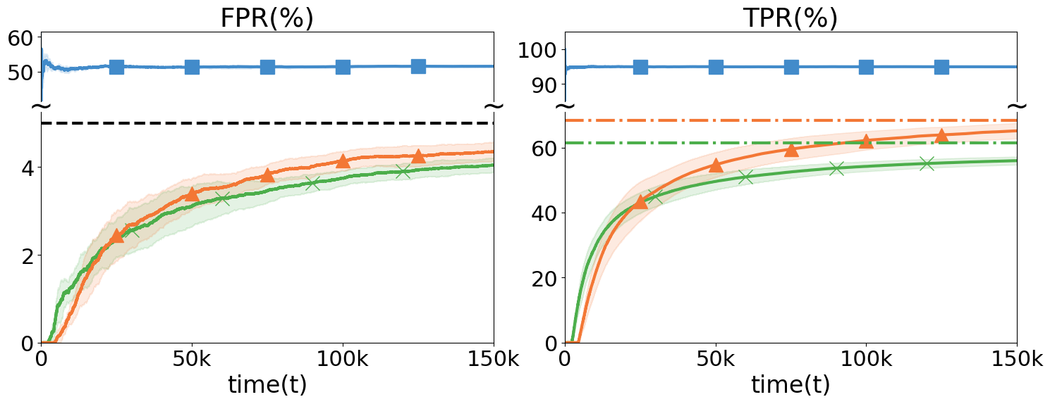
(c) Stationary, KNN, CIFAR-100 as OOD.

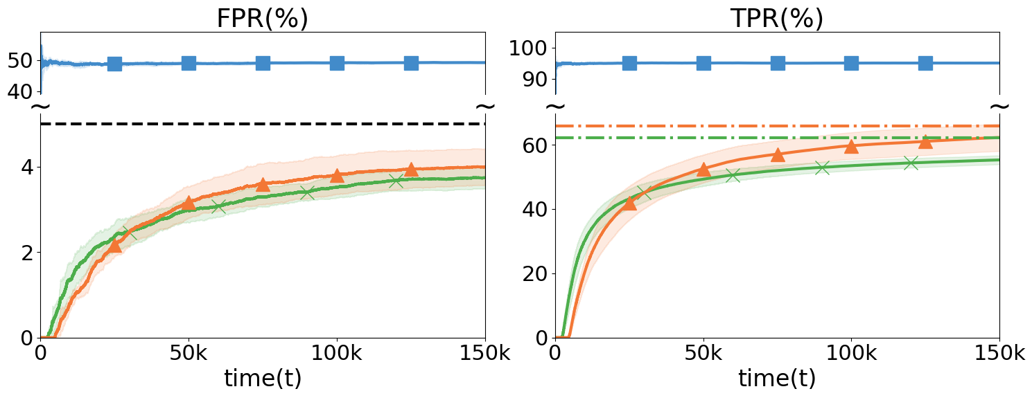
(d) Stationary, KNN, Near-OOD as OOD.

Figure 5: Results on the stationary setting for CIFAR-10 as ID, with each method repeated 5 times (mean and std shown). EBO and KNN are the initial scoring functions and are fixed for FSFT and FSAT. The dotted-dash lines represent the expected TPR at FPR-5% for EBO, KNN, and $\widehat{g}^{\ast}$ (matching colors).

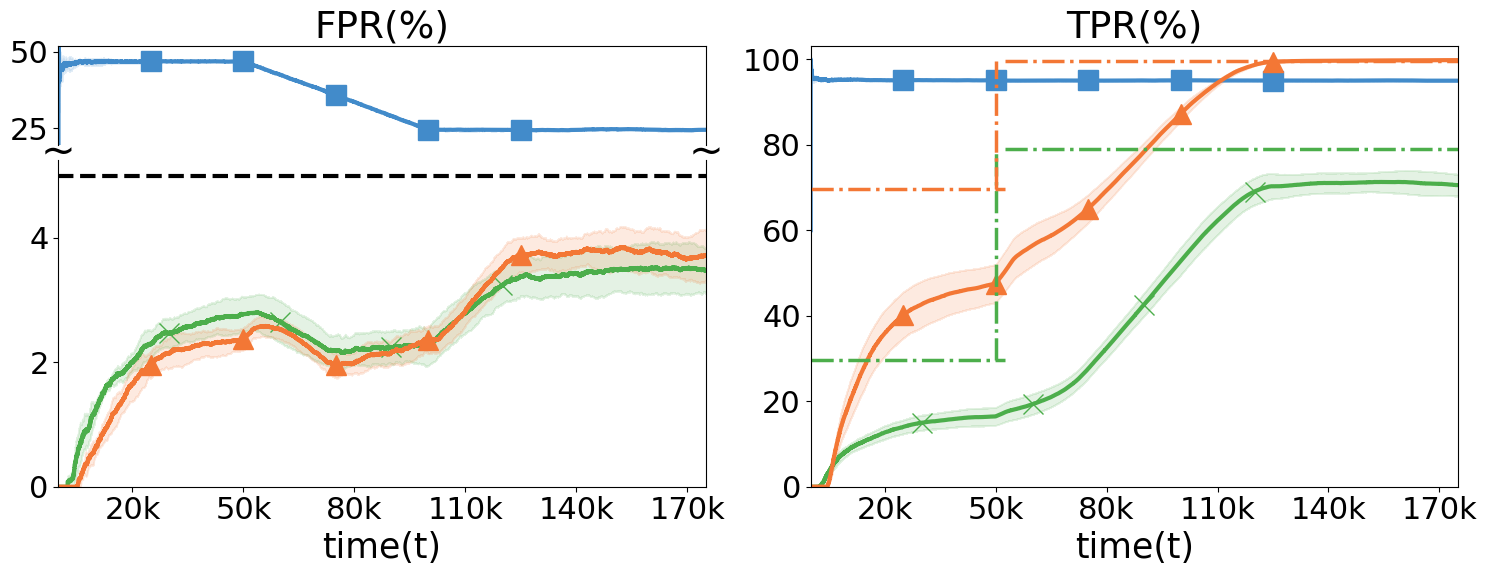
(a) EBO, 5k window, From Near-OOD to Far-OOD.

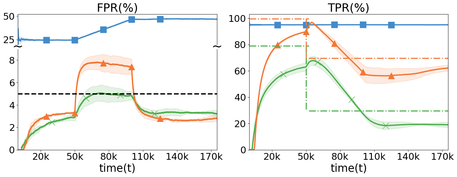
(b) EBO, 5k window, From Far-OOD to Near-OOD.

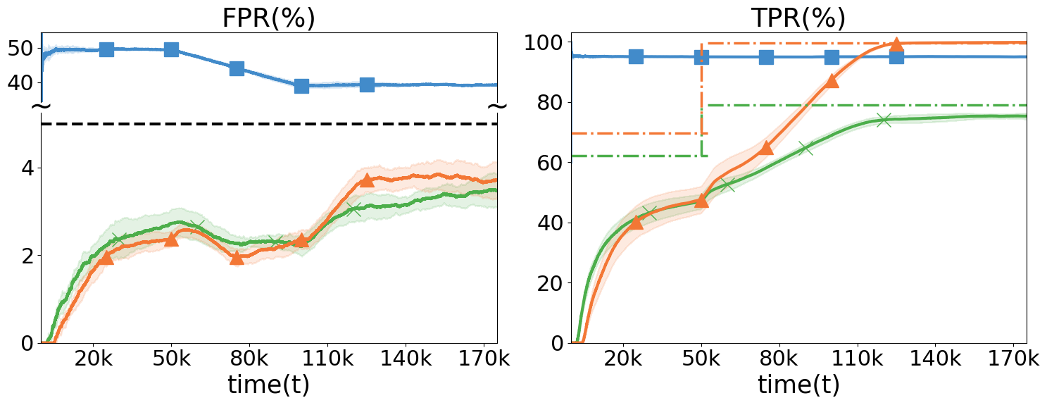
(c) KNN, 5k window, From Near-OOD to Far-OOD.

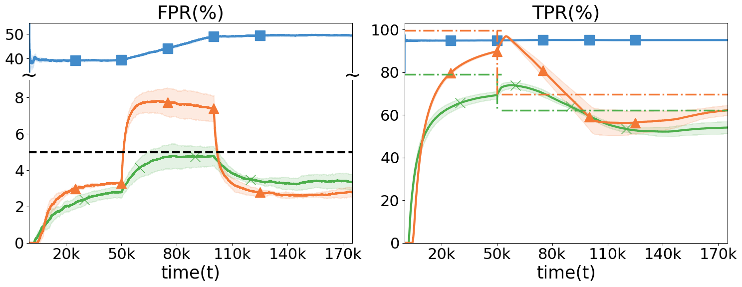
(d) KNN, 5k window, From Far-OOD to Near-OOD.

Figure 6: Results on the nonstationary setting, with each method repeated 5 times (mean and std shown). A shift happens between Near-OOD and Far-OOD mixtures at time $t=$ 50k. EBO and KNN are the initial scoring functions and are fixed for FSFT and FSAT. The dotted-dash lines represent the TPR at FPR-5% for EBO, KNN, and $\widehat{g}^{\ast}$ (matching colors).

4 Theoretical Analysis

We provide a theoretical analysis of FPR control in stationary settings, where both $\mathcal{D}_{0}$ and $\mathcal{D}_{1}$ remain fixed over time (but unknown). Our goal is to show that ASAT maintains $\mathrm{FPR}(\widehat{g}_{t},\widehat{\lambda}_{t})<\alpha$ at all times. The result is presented below.

Proposition 1.

Let $U_{t}$ be the total number of updates before time $t$. Let $N_{t}^{(o)}=\sum_{u=1}^{t}Z_{u}$, and $N_{t}^{(imp)}$ be the number of importance sampled OOD points. Define $\beta_{t}=N_{t}^{(imp)}/N_{t}^{(o)}$, $c_{t}=1+(1-p)\beta_{t}/p^{2}$, and $t_{0}=\min\{u:c_{u}N_{u}^{(o)}\geq 173\log(4/\delta)\}$. Let $\Lambda:=\{\Lambda_{\min},\Lambda_{\min}+\eta,\ldots,\Lambda_{\max}\}$, with discretization parameter $\eta>0$. Then, w.p. at least $1-\delta$, we have $\forall\;t\geq t_{0}$,

1. $\sup\limits_{\lambda\in\Lambda}\left|\widehat{\mathrm{FPR}}_{t}(\widehat{g}_{t},\lambda)-\mathrm{FPR}(\widehat{g}_{t},\lambda)\right|\leq\psi_{t}(\delta),\text{where}$

   $$\psi_{t}(\delta):=\sqrt{\frac{3c_{t}}{N_{t}^{(o)}}\left[2\log\log\left(\frac{3c_{t}N_{t}^{(o)}}{2}\right)+2\log\left(\frac{4U_{t}|\Lambda|}{\delta}\right)\right]}.$$

2. Consequently, $\mathrm{FPR}(\widehat{g}_{t},\widehat{\lambda}_{t})\leq\alpha$.

Interpretation. Proposition 1 establishes the desired FPR control at all times in ASAT. It ensures that w.p. at least $1-\delta$, a) the FPR estimate (2) is within $\psi_{t}(\delta)$ of the true FPR for all $t$ and $\lambda$, and consequently b) $\text{FPR}\leq\alpha$ in ASAT.

Discussion. Similar results were obtained for FSAT (which adapts thresholds for a fixed scoring function) using a similar UCB (Vishwakarma et al., 2024c). But, this approach does not extend directly to our setting, where ASAT also updates scoring functions and uses them for predictions and sample collections. Nevertheless, our design achieves comparable FPR control and higher TPR—since ASAT optimizes scoring functions to maximize TPR in (P2).

However, these advantages come with a slight trade-off: $\psi_{t}(\delta)$ includes the additional $U_{t}$ term to ensure that it is also valid for time-varying $\widehat{g}_{t}$. In practice, we anticipate $U_{t}\ll N_{t}^{(o)}$, since updates occur only periodically. Thus, this extra dependence on $U_{t}$ results only in a minor increase in $\psi_{t}(\delta)$ from FSAT, which is offset by the improved TPR.

Proof Sketch. The proof of Proposition 1 entails challenges. First, the samples used to estimate the FPR in eq (2) are dependent. In particular, whether we receive the human label for $x_{t}$ depends on the previously learned scoring function $\widehat{g}_{t-1}$ and threshold $\widehat{\lambda}_{t-1}$, both of which are functions of previous data $\{x_{1},...,x_{t-1}\}$. This dependency prevents the direct application of the i.i.d. LIL bound (Howard and Ramdas, 2022). To overcome this, we leverage the martingale structure of our data and apply the martingale LIL bound (Khinchine, 1924; Balsubramani, 2015), yielding a time-uniform confidence sequence. Additionally, we ensure that these confidence intervals hold simultaneously for all $\lambda\in\Lambda$ and all deployed scoring functions by applying the union bound. See Appendix C for detailed proofs.

5 Experiments

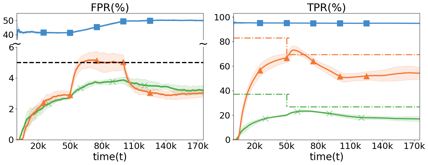
(a) EBO, 5k window.

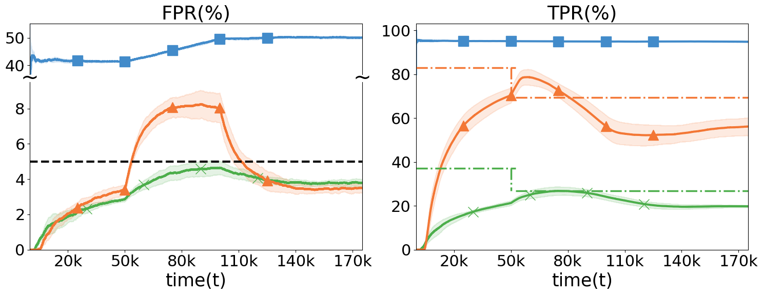
(b) EBO, 10k window.

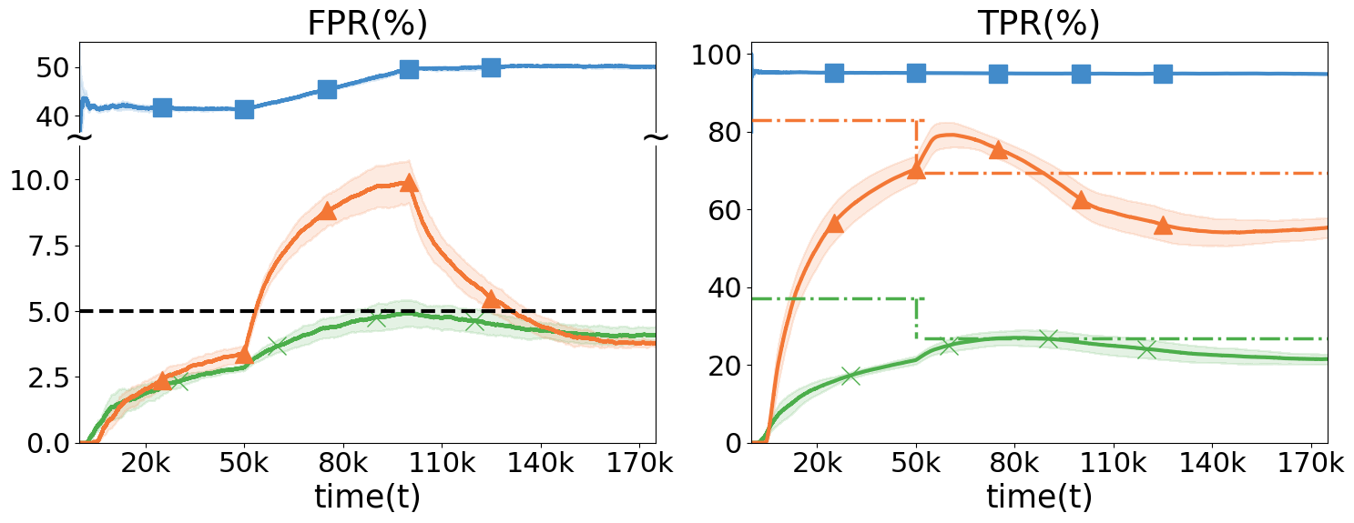
(c) EBO, 15k window

Figure 7: Results on the nonstationary setting with different window sizes 5k, 10k, and 15k, with each method repeated 5 times (mean and std shown). A shift happens from Places365 and CIFAR-100 at time $t=$ 50k.

We compare three methods: FSFT (fixed scoring functions and thresholds), FSAT (fixed scoring functions with adaptive thresholds), and our proposed ASAT (adaptive scoring functions and thresholds). We verify the following claims on OpenOOD benchmarks.

C1. In stationary settings, ASAT (ours) $\succ$ FSAT $\succ$ FSFT, where $a\succ b$ means that method $a$ achieves better TPR than $b$ while maintaining FPR below $\alpha$, or that $b$ violates the FPR constraint.

C2. ASAT adapts to nonstationary OOD settings, updating scoring functions and thresholds to maximize TPR with minimal FPR violations.

For completeness, we also compare ASAT against a naive binary classifier in Appendix D.1.

5.1 Experiment Settings

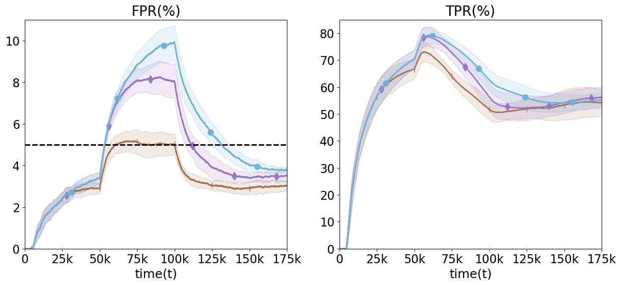
Figure 8: Results on nonstationary OOD from Places365 to CIFAR-100 with different window $N^{(est)}_{w}$; only ASAT results are shown.

Datasets. We use CIFAR-10 (Krizhevsky et al., 2009) as ID for the experiments. In stationary settings, we use CIFAR-100 and a mixture of CIFAR-100, Tiny-ImageNet (Deng et al., 2009), Places365 (Zhou et al., 2017) as OOD (referred to as Near-OOD). In nonstationary settings, we change the distribution at time $t=50$k for all experiments. We use pairs of (1) CIFAR-100 and Places365 and (2) a mixture of MNIST (Deng, 2012), SVHN, and Texture (referred to as Far-OOD) and a mixture of CIFAR-100, Tiny-ImageNet, and Places365 (Near-OOD).

See Appendix D.6 and D.7 for additional experiments on different feature extractor (ViT-B/16 (Dosovitskiy et al., 2021)), ID datasets (CIFAR-100, ImageNet-1k (Deng et al., 2009)), OOD datasets, and scoring functions.

Scoring Functions. We use post-processing scoring functions based on a ResNet18 model (He et al., 2016), which is trained on CIFAR-10, from Open-OOD benchmarks: ODIN (Liang et al., 2018), Energy Score (EBO) (Liu et al., 2020), KNN (Sun et al., 2022), Mahalanobis Distances (MDS) (Lee et al., 2018a), and VIM (Wang et al., 2022). Both FSFT and FSAT used a fixed scoring function from the above benchmarks. For consistency, in ASAT, the same initial scoring function as FSFT is used until enough OOD samples are identified and the first update occurs.

Evaluation FPR and TPR. For evaluation, we count the actual number of false-positive and true-positive instances incurred by a method within a specific time frame. These evaluation FPR and TPR are defined as

$$\text{FPR}^{(eval)}_{t} =\frac{\sum_{u=t^{\prime}}^{t}\mathbbm{1}\{y_{u}=0,\widehat{y}_{u}=1\}}{\sum_{u=t^{\prime}}^{t}\mathbbm{1}\{y_{u}=0\}},$$ (7)

$$\text{TPR}^{(eval)}_{t} =\frac{\sum_{u=t^{\prime}}^{t}\mathbbm{1}\{y_{u}=1,\widehat{y}_{u}=1\}}{\sum_{u=t^{\prime}}^{t}\mathbbm{1}\{y_{u}=1\}},$$

where $t^{\prime}=t-N_{w}^{(eval)}$, and $N_{w}^{(eval)}$ denotes the window size of past instances used for evaluation.

Choices of $\mathcal{G}$. Our framework is flexible with the choice of $\mathcal{G}$. We use 2-layer ReLU neural networks that take a feature output from the penultimate layer of the Resnet18. To solve (P2), we use the Adam optimizer (Kingma and Ba, 2014). See Appendix D.3 for more details.

Hyperparameters and Constants. We perform a grid search to optimize our hyperparameters. In particular, we set $\beta=1.5$ and $\kappa=50$. For the constants, we use $\alpha=0.05$, $\gamma=0.2$, and $p=0.2$ (See Appendix D.4).

Empirical Convergence to Optimality. We assess convergence of $(\widehat{g}_{t},\widehat{\lambda}_{t})$ by comparing $\mathrm{TPR}^{(eval)}_{t}$ (7) with the reference $\mathrm{TPR}(\widehat{g}^{\star},\lambda)$. Here, $(\widehat{g}^{\star},\lambda)$ is near-optimal for (P1), where $\widehat{g}^{\star}$ is trained on i.i.d. OOD/ID data, and $\lambda$ is chosen to satisfy $\text{FPR}(\widehat{g}^{\star},\lambda)=\alpha$. Intuitively, $\mathrm{TPR}(\widehat{g}^{\star},\lambda)$ represents the best achievable TPR under $\text{FPR}\leq\alpha$, and we expect $\mathrm{TPR}^{(eval)}_{t}$ to converge toward it as $t$ increases in ASAT.

Thresholds for Baselines. While FSFT uses a fixed threshold at TPR-95%, both FSAT and ASAT update thresholds over time. For FSAT, we adopt the same heuristic UCB from Vishwakarma et al. (2024c). For ASAT  we adapt the theoretical bound in (6) as

$$\psi^{H}_{t}(\delta):=c_{1}\sqrt{\frac{c_{t}}{N_{t}^{(o)}}\left[\log\log\left(c_{2}c_{t}N_{t}^{(o)}\right)+\log\left(\frac{c_{3}}{\delta}\right)\right]},$$

with $c_{1}=0.65$, $c_{2}=0.75$, and $c_{3}=1.0$. Here, $c_{2}$ and $c_{3}$ are set as in Vishwakarma et al. (2024c), while $c_{1}$ is increased to account for the varying score functions (see Section 4). See Appendix D.2 for more details.

Stationary Setting. In this setting, $\mathcal{D}_{0}$ and $\mathcal{D}_{1}$ remain fixed. For evaluation, we set $N_{w}^{(eval)}=t$ (i.e., using all past data), since no abrupt changes in FPR/TPR are anticipated. For updating $\widehat{g}_{t}$, we set the optimization frequency $\omega^{(ood)}_{i}$ to 100 for the first 2k OOD points, 500 for the next 10k, and 1000 thereafter. This allows aggressive updates early on, with update frequency decreasing as $\widehat{g}_{t}$ becomes better trained.

Nonstationary Setting. We manually change the OOD $\mathcal{D}_{0}$ at $t=50k$, since variations in $\gamma$ or $\mathcal{D}_{1}$ do not impact the FPR. We set $N_{w}^{(eval)}=50$k for a more optimistic performance metric and use $\omega^{(ood)}_{i}=100$ for the first 2k samples and 500 afterward to ensure $\widehat{g}_{t}$ adapts quickly to the new OOD. Since using all the past OOD samples (including outdated ones) becomes ineffective after a shift, we adopt a windowed approach that relies only on the most recent $N_{w}^{(est)}$ OOD samples for FPR estimation and updating $\widehat{g}_{t}$. This enables quicker adaptation to the new distribution. Note that the window size presents a trade-off: a smaller window encourages faster adaptation but results in a wider confidence interval, which in turn limits optimality.

5.2 Results and Discussions

C1. In stationary settings, ASAT aims to control FPR while maximizing TPR. In Figure 5, FSFT exhibits very high FPR at TPR-95%, whereas both FSAT and ASAT keep FPR consistently below 5% across all four settings. Initially, both FSAT and ASAT yield a TPR of 0% because insufficient OOD samples force $\widehat{\lambda}_{t}$ to be set to $\infty$ (as per Q1), until enough OOD samples are collected to satisfy $\psi_{t}(\delta)\leq\alpha$. Moreover, ASAT initially achieves a lower TPR than FSAT because it adapts both thresholds and scoring functions—resulting in a wider confidence bound $\psi_{t}(\lambda)$ that requires more OOD samples—while FSAT updates only thresholds (see Section 4).

However, this early drawback is offset by its ability to maximize TPR later in deployment. ASAT quickly catches up with FSAT and eventually surpasses the best achievable TPR by FSAT at FPR-5% in all settings. In particular, when both methods start with EBO, ASAT shows over a 40% improvement in TPR towards the end (see Figures 15(a) and 15(b)). As expected, $\mathrm{TPR}(\widehat{g}_{t},\widehat{\lambda}_{t})$ converges to $\mathrm{TPR}(\widehat{g}^{\star},\lambda)$, confirming optimality. The stationary results verify that ASAT effectively updates both scoring functions and thresholds to maximize TPR while ensuring FPR control, outperforming the baselines.

C2. In nonstationary settings, ASAT aims to maximize TPR while minimizing FPR violation if it occurs. As shown in Figure 6, FPR violations occur when the new OOD is less distinguishable from the ID than the old OOD (e.g., Far-OOD to Near-OOD in Figures 6(b) and 6(d)) whereas no FPR violations are observed in the reverse shift (Figures 6(a) and 6(c)). In Figure 7, ASAT initially shows larger FPR violations than FSAT, which is expected since it adapts (or specializes) the scoring functions based on previous OOD data. However, ASAT quickly reduces FPR below $\alpha$ and effectively adapts to the new OOD, consistently achieving higher TPR than FSAT both before and after the shift.

Finally, Figure 8 illustrates that smaller windows enable faster adaptation and reduce FPR violations, although they limit the convergence of TPR.

6 Related Works

OOD Detection. Robustness to out-of-distribution (OOD) data has been extensively studied in recent years (Salehi et al., 2022; Yang et al., 2024). Various post-hoc and training-time methods have been proposed to learn scoring functions for OOD detection (Bendale and Boult, 2015; Hendrycks and Gimpel, 2017; Liu et al., 2020; Wang et al., 2022; Sehwag et al., 2021; Ming et al., 2023; Ren et al., 2019; Kirichenko et al., 2020; DeVries and Taylor, 2018; Chen et al., 2021; Huang and Li, 2021; Wei et al., 2022). However, most approaches rely solely on ID data to design scoring functions and set score thresholds, focusing on maximizing TPR. This approach often results in a high FPR. Furthermore, fixed scoring functions and thresholds limit a system’s ability to adapt to varying OOD inputs. A few recent works proposed offline solutions to train the classification model along with an OOD detector using an unlabeled mixture of ID and OOD data (Katz-Samuels et al., 2022) or with a few labeled samples obtained using active learning (Bai et al., 2024). In our setting, we need an online solution to adapt to unforeseen variations in the OOD data while maintaining strict control on the false positive rate.

FPR Control for OOD Detection. Some of these challenges were addressed by Vishwakarma et al. (2024c), who introduced a method that adapts thresholds over time—while using a fixed scoring function—to ensure FPR control. Although effective in controlling FPR, a fixed scoring function restricts the achievable TPR. Our work extends this approach by jointly learning scoring functions and thresholds to explicitly maximize TPR subject to an FPR constraint, using OOD inputs collected via human feedback during deployment. Similar ideas have been explored in model-assisted data labeling (Vishwakarma et al., 2023, 2024b, 2024a) and in optimizing set sizes for conformal prediction (Stutz et al., 2022).

Time-uniform Confidence Sequences. Our method leverages time-uniform confidence sequences based on the Law-of-Iterated Logarithms (LIL) from multi-armed bandits literature (Darling and Robbins, 1967; Lai, 1976; Jamieson et al., 2014; Howard and Ramdas, 2022), which have been used in active learning for ranking and clustering settings Heckel et al. (2019); Vinayak (2018); Chen et al. (2023). However, these anytime confidence intervals are often constructed under i.i.d assumptions. Due to importance sampling with time-varying scoring functions and thresholds, the samples are no longer i.i.d in ASAT. We address this by constructing a martingale sequence and building on the martingale-LIL result by Balsubramani (2015) to derive time-uniform confidence sequences suitable for our setting.

7 Conclusion

We introduced a human-in-the-loop OOD detection framework that updates both scoring functions and thresholds to maximize TPR while strictly controlling FPR. Our approach formulated this as a constrained joint optimization problem, with a relaxed version developed for practical learning. To guarantee FPR control throughout deployment, we designed novel time-uniform confidence sequences that account for dependencies from importance sampling and time-varying scores and thresholds. Empirical evaluations demonstrate that our approach consistently outperforms methods that use fixed scoring functions by maintaining FPR control and improving TPR.

8 Limitations and Future Work

While ASAT provides a new adaptive OOD detection framework with formal FPR control guarantees, several limitations remain and motivate future work.

Noisy Human Feedback. ASAT currently assumes accurate human labels but can potentially be extended to handle noisy feedback using techniques from the label noise literature, such as the unbiased estimators proposed by Natarajan et al. (2013). Incorporating such corrections into FPR estimation and extending FPR guarantees under noisy labels is a promising direction for future work.

Shift Detection for Nonstationary Settings. Our guarantees assume stationary OOD distributions. A possible extension is to use change-point detection (e.g., by monitoring FPR) to detect shifts and re-initialize ASAT, which allows the stationary guarantees to apply piecewise across each stationary interval. A full theoretical analysis under nonstationary settings is left for future work.

Different Types of Distribution Shifts. ASAT focuses on semantic OOD shifts, but covariate shifts (e.g., noise, resolution changes) are also important. Evaluating and extending ASAT under such shifts is an open area for future research.

9 Acknowledgment

We thank Frederic Sala and Thomas Zeng for their valuable inputs. We thank the anonymous reviewers for their valuable comments and constructive feedback on our work.

Appendix

The appendix is organized as follows. We provide a summary of the variables and constants in Table 1. Then, we give an algorithm for the entire ASAT workflow in Section B and detailed proofs for the FPR control in Section C. In Section D, we provide additional experimental results and details of the experiment protocol and hyperparameters used for the experiments.

Appendix A Glossary

We provide the following list of variables and constants used in our framework (Table 1).

Symbol	Definition/Description
$\mathcal{X}$	feature space.
$\mathcal{Y}$	label space $\{0,1\}$, 0 for OOD and 1 for ID.
$\mathcal{D}_{0},\mathcal{D}_{1}$	the underlying distributions of OOD and ID points
$\gamma$	mixture ratio of OOD and ID distributions.
$x_{t},s_{t},y_{t},\widehat{y}_{t}$	sample, score, true label, and predicted label at time $t$.
$X_{t}^{(ood)}$.	dependent OOD samples collected up to time $t$.
$X_{0}^{(id)}$	i.i.d. ID samples available before deployment.
$\mathrm{FPR}(g,\lambda)$	population level false positive rate defined by scoring function $g$ and threshold $\lambda$.
$\mathrm{TPR}(g,\lambda)$	population level true positive rate defined by scoring function $g$ and threshold $\lambda$.
$\widehat{\mathrm{FPR}}_{t}(g,\lambda)$	estimated FPR at time $t$, adjusted to account for importance sampling (see eq. (2)).
$\widehat{\mathrm{TPR}}(g,\lambda)$	estimated TPR fixed for all $t$, based on i.i.d. ID points (see eq. (3)).
$\widetilde{\text{FPR}}_{t}(g,\lambda)$	smoothed $\widehat{\mathrm{FPR}}_{t}(g,\lambda)$ (see eq. (4)) used for optimization in eq. (P2)
$\widetilde{\text{TPR}}(g,\lambda)$	smoothed $\widehat{\mathrm{TPR}}(g,\lambda)$ (see eq. (5)) used for optimization in eq. (P2).
$\text{FPR}_{t}^{(eval)}$	evaluation FPR for experiments in eq. (7).
$\text{TPR}_{t}^{(eval)}$	evaluation TPR for experiments in eq. (7).
$\mathcal{G},\Lambda$	hypothesis class of scoring functions over $\mathcal{X}$ and space of thresholds.
$(g^{\ast},\lambda^{\ast})$	the optimal solution (non-unique) to the joint optimization problem in eq. (P1).
$(\widehat{g}_{t},\widehat{\lambda}_{t})$	scoring function and threshold learned at time $t$.
$\widehat{\lambda}_{t}^{\prime}$	unsafe threshold obtained from eq. (P1) together with $\widehat{g}_{t}$.
$i_{u}$	indicator of whether $x_{t}$ was importance sampled.
$\sigma(\kappa,z)$	sigmoid function for input $z$.
$\omega^{(ood)}_{i}$	optimization frequency, indicating the number of new OOD points required for $i$th updating.
$\beta_{t},c_{t}$	time-dependent variables used for LIL-based confidence bounds (see Proposition 1).
$\Delta_{t}^{(ood)}$	number of new OOD points identified via human feedback up to time $t$ since last update.
$N_{t}^{(imp)}$	number of OOD points identified via importance sampling up to time $t$.
$U_{t}$	number of total deployments of new scoring functions by time $t$.
$N_{w}^{(eval)}$	window size that the system uses for computing evaluation FPR and TPR.
$N_{w}^{(est)}$	window size for estimation and optimization for nonstationary OOD settings.
$p$	importance sampling probability.
$\delta$	failure probability for confidence intervals.
$\alpha$	the threshold for FPR for all time points.
$\eta$	discretization parameter for $\Lambda$.
$\beta$	optimization parameter that controls a trade-off between TPR and FPR.
$\kappa$	the smoothness parameter of sigmoid functions
$(c_{1},c_{2},c_{3})$	constants use for heuristic LIL bounds.
$\psi_{t}(\delta)$	LIL-based confidence interval at time $t$.
$\psi^{H}_{t}(\delta)$	LIL-based heuristic interval at time $t$.
$\zeta(\delta,n)$	DKW confidence interval for TPR.

Table 1: Glossary of variables and symbols used in the framework.

Appendix B Additional Details for Methodology

We provide a detailed description of the ASAT workflow in Algorithm 1. We also provide the algorithm for binary search procedures used to solve (Q1) in Algorithm 2.

Algorithm 1 ASAT (Adaptive Scoring function, Adaptive Threshold)

1:procedure ASAT($\alpha$, $p$, $\delta$, $\beta$, $\widehat{g}_{0}$, $\{\omega^{(ood)}_{i}\}_{i\geq 0}$, $X_{0}^{(id)}$)

2:  $\widehat{\lambda}_{0}\leftarrow+\infty$, $X_{0}^{(ood)}\leftarrow\emptyset,U_{0}\leftarrow 1$.

3:  $\Delta_{0}^{(ood)}\leftarrow 0$ (# new OOD identified via human labels since last update)

4:  for $t=1,2,\dots$ do

5:   Observe $x_{t}$

6:   Compute $s_{t}\leftarrow\widehat{g}_{t-1}(x_{t})$

7:   if $s_{t}\leq\widehat{\lambda}_{t-1}$ then $\triangleright$ $x_{t}$ is predicted as OOD

8:     $l_{t}\leftarrow 1$ $\triangleright$ $l_{t}=1$ w.p. 1

9:   else$\triangleright$ $x_{t}$ is predicted as ID

10:     $l_{t}\sim\text{Bern}(p)$ $\triangleright$ $l_{t}=1$ w.p. $p$

11:   end if

12:   if $l_{t}=1$ then

13:     $y_{t}=$ GetHumanLabel$(x_{t})$ $\triangleright$ Obtain human label $y_{t}$ if $l_{t}=1$

14:     if $y_{t}=0$ then $\triangleright$ If $x_{t}$ is truly OOD

15:      $X_{t}^{(ood)}\leftarrow X_{t-1}^{(ood)}\cup x_{t}$ $\triangleright$ Add $x_{t}$ to the set of OOD

16:      $\Delta_{t}^{(ood)}\leftarrow\Delta_{t}^{(ood)}+1$

17:     end if

18:   end if

19:   $\color[rgb]{.5,.5,.5}\triangleright$ Learn new scoring function

20:   if $\Delta_{t}^{(ood)}\geq\omega^{(ood)}_{U_{t}}$ then $\triangleright$ If we have collected enough new OOD samples

21:     $i\leftarrow i+1$,  $\Delta_{t}^{(ood)}\leftarrow 0$

22:     $\widehat{g}_{t},\widehat{\lambda}_{t}^{\prime}\leftarrow\operatorname*{arg\,min}\limits_{g\in\mathcal{G},\lambda\in\Lambda}-\widetilde{\text{TPR}}(g,\lambda)+\beta\cdot\widetilde{\text{FPR}}_{t}(g,\lambda)\quad$ using $X_{t}^{(ood)}$ and $X_{0}^{(id)}$ (P2)

23:     $\color[rgb]{.5,.5,.5}\triangleright$ Estimate threshold

24:     $\widehat{\lambda}_{t}\leftarrow\operatorname*{arg\,min}\limits_{\lambda\in\Lambda}\lambda\quad\text{s.t.}\quad\widehat{\text{FPR}}_{t}(\widehat{g}_{t},\lambda)+\psi_{t}(\delta)\leq\alpha\quad$ via BinarySearch($X_{t}^{(ood)}$, $\widehat{g}_{t}$) (Q1)

25:     

26:     $\color[rgb]{.5,.5,.5}\triangleright$ Model selection

27:     if $\widehat{\text{TPR}}(\widehat{g}_{t},\widehat{\lambda}_{t})+2\zeta(\delta,|X_{0}^{(id)}|)>\widehat{\text{TPR}}(\widehat{g}_{t-1},\widehat{\lambda}_{t-1})$ then $\triangleright$ If the model selection criterion is satisfied

28:      $\widehat{g}_{t}\leftarrow\widehat{g}_{t}$ $\triangleright$ Deploy the new scoring function

29:      $\widehat{\lambda}_{t}\leftarrow\widehat{\lambda}_{t}$ $\triangleright$ Update to the new threshold

30:      $U_{t}\leftarrow U_{t-1}+1$

31:     else

32:      $\widehat{g}_{t}\leftarrow\widehat{g}_{t-1}$ $\triangleright$ Retain the old scoring function

33:      $U_{t}\leftarrow U_{t-1}$

34:     end if

35:   end if

36:   if $g$ is not updated then

37:     $\color[rgb]{.5,.5,.5}\triangleright$ Estimate threshold

38:     $\widehat{\lambda}_{t}\leftarrow\operatorname*{arg\,min}\limits_{\lambda\in\Lambda}\lambda\quad\text{s.t.}\quad\widehat{\text{FPR}}_{t}(\widehat{g}_{t},\lambda)+\psi_{t}(\delta)\leq\alpha\quad$ via BinarySearch($X_{t}^{ood}$, $\widehat{g}_{t}$) (Q1)

39:   end if

40:   if $l_{t}=1$ then

41:     Output $y_{t}$ $\triangleright$ Output the true label obtained via human feedback

42:   else

43:     Output $\widehat{y_{t}}:=\mathbbm{1}\{s_{t}>\widehat{\lambda}_{t-1}\}$ $\triangleright$ Output predicted label via one-sided threshold function

44:   end if

45:  end for

46:end procedure

Algorithm 2 Binary Search to Solve (Q1)

1:procedure BinarySearch($X_{t}^{(ood)}$, $\widehat{g}_{t}$)

2:  $\lambda_{l}=\Lambda_{min}$, $\lambda_{h}=\Lambda_{max}$, $feasible=$ False, $\epsilon\approx 0$

3:  while $\lambda_{h}-\lambda_{l}>\epsilon$ do

4:   $\lambda_{m}=(\lambda_{l}+\lambda_{h})/2$

5:   if $\widehat{\text{FPR}}_{t}(\widehat{g}_{t},\lambda_{m})+\psi_{t}(\delta)\leq\alpha$ then

6:     $feasible=$ True

7:     $\lambda_{h}=\lambda_{m}$

8:   else

9:     $\lambda_{l}=\lambda_{m}$

10:   end if

11:  end while

12:  return $\lambda_{m}$, $feasible$

13:end procedure

DKW Criterion for Model Selection. Suppose an update occurs at time $t$ (i.e., $\Delta^{ood}_{t}\geq\omega^{ood}_{U_{t}}$) by solving (P2). We ensure that the updated scoring function $\widehat{g}_{t}$ outperforms $\widehat{g}_{t-1}$, by applying following TPR criterion:

$$\widehat{\text{TPR}}(\widehat{g}_{t},\widehat{\lambda}_{t})+2\zeta(\delta,|X_{0}^{(id)}|)>\widehat{\text{TPR}}(\widehat{g}_{t-1},\widehat{\lambda}_{t-1}),$$

where $\zeta(\delta,|X_{0}^{(id)}|)$ is the Dvoretzky–Kiefer–Wolfowitz (DKW) confidence interval (Nadaraya, 1965) given by

$$\zeta(\delta,|X_{0}^{(id)}|)=\sqrt{\frac{1}{|X_{0}^{(id)}|}\log\left(\frac{2}{\delta}\right)},$$

which is valid w.p. at least $1-\delta$. This confidence bound relies on the fact that $X_{0}^{(id)}$ is i.i.d. and the TPR can be expressed as $\text{TPR}(g,\lambda)=1-F_{1}(\lambda;g)$, where $F_{1}$ is the CDF of the ID score distribution mapped by $g$.

Appendix C Proofs

Summary of ASAT Settings. At each time $t$, the ASAT system processes an input $x_{t}$ using scoring function $\widehat{g}_{t-1}$ and threshold $\widehat{\lambda}_{t-1}$, both learned at the previous time $t-1$. It first computes score $s_{t}=\widehat{g}_{t-1}(x_{t})$ for $x_{t}$. If $s_{t}<\widehat{\lambda}_{t-1}$, then $x_{t}$ is considered OOD and receives a human label $y_{t}\in\{0,1\}$. If $s_{t}\geq\widehat{\lambda}_{t-1}$, $x_{t}$ is considered ID, and in this case, we obtain the human label $y_{t}$ only with probability $p\in(0,1)$ (i.e., importance sampling). Now, if $x_{t}$ is identified as OOD and the system has collected enough new OOD points required for the next update (i.e., $\Delta^{(ood)}_{U_{t}}$), we estimate the FPR and TPR (1) using the collected finite samples to solve the optimization in (P2).

The FPR and TPR estimates are defined as

$$\widehat{\text{FPR}}_{t}(g,\lambda)=\frac{\sum_{u=1}^{t}Z_{u}\cdot\mathbbm{1}\{g(x_{u})>\lambda\}}{\sum_{u=1}^{t}Z_{u}},$$ (8)

$$Z_{u}:=\begin{cases}1&\text{if }s_{u}<\widehat{\lambda}_{u-1},i_{u}=0,y_{u}=0,\\ \frac{1}{p}&\text{if }s_{u}\geq\widehat{\lambda}_{u-1},i_{u}=1,y_{u}=0,\\ 0&\text{otherwise},\end{cases}$$

and

$$\widehat{\text{TPR}}(g,\lambda) =\frac{1}{|X_{0}^{(id)}|}\sum_{x\in X_{0}^{(id)}}\mathbbm{1}\{g(x)\geq\lambda\}.$$ (9)

In (P2), the differentiable surrogates of the FPR and TPR estimates from (4) and (5) are used for efficient optimization. If an update occurs, the system obtains a new scoring function $\widehat{g}_{t}$ and threshold $\widehat{\lambda}_{t}^{\prime}$. Otherwise, the previous scoring function is retained, i.e., $\widehat{g}_{t}=\widehat{g}_{t-1}$. Since the optimization problem in (P2) is unconstrained, there’s no guarantee that the original FPR constraint will be satisfied by $\widehat{g}_{t}$ and $\widehat{\lambda}_{t}^{\prime}$. Therefore, the system solves a different optimization in (Q1) to find $\widehat{\lambda}_{t}$, replacing $\widehat{\lambda}_{t}^{\prime}$, based on the current scoring function $\widehat{g}_{t}$. In this optimization, we use the FPR estimate in eq (2) and LIL-based upper confidence bounds (UCB) to ensure that the true FPR constraint is satisfied with high probability. Additional details on the workflow are provided in B.

Proof Outline. Our goal in ASAT is to ensure that $\mathrm{FPR}(\widehat{g}_{t},\widehat{\lambda}_{t})$ remains below $\alpha$ at all times. Similar results were achieved for FSAT, where thresholds were adapted for a fixed scoring function (Vishwakarma et al., 2024c). Their results relied on constructing time-uniform FPR estimation bounds for all times $t$ and thresholds $\lambda\in\Lambda$. The OOD samples used to estimate the FPR are non-i.i.d., as the decision to receive a human label for $x_{t}$ depends on the previously learned $\widehat{g}_{t-1}$ and $\widehat{\lambda}_{t-1}$, which themselves are functions of past data $\{x_{1},\dots,x_{t-1}\}$. In FSAT, this dependency is handled by applying the martingale version of the LIL bound (Khinchine, 1924; Balsubramani, 2015), which leads to a time-uniform confidence sequence.

However, in ASAT, the same LIL-based UCB does not directly apply, as the system periodically adapts new, time-varying, scoring functions and uses them for predictions and sample collection. Despite this, we claim that our design still ensures comparable FPR control. We first show that each $x_{t}$ identified as OOD is an unbiased estimator for the FPR.

Lemma 1.

Let $Z_{u}$ be defined as in eq (2), and let $i_{u}$ be the indicator for whether $x_{u}$ is importance sampled. Given $g\in\mathcal{G}$ and $\lambda\in\Lambda$, we have

$$\mathbb{E}_{x_{u},i_{u}}[Z_{u}\mathds{1}\{g(x_{u})\geq\lambda)\}]=\mathrm{FPR}(g,\lambda).$$

Proof.

Let $m_{u}=\mathbb{P}\left(\widehat{g}_{u-1}(x_{u})<\widehat{\lambda}_{u-1}\right)$.

$$\begin{split}\mathbb{E}_{x_{u},i_{u}}\left[Z_{u}\mathds{1}\{g(x_{u})\geq\lambda)\}\right]&=\mathbb{E}_{x_{u}}\left[\mathds{1}\{g(x_{u})\geq\lambda)\}\mathbb{E}_{i_{u}|x_{u}}\left[Z_{u}\right]\right].\end{split}$$

Conditioned on $x_{u}$, we have

$$\mathbb{E}_{i_{u}|x_{u}}\left[Z_{u}\right] =\mathbb{P}(\widehat{g}_{u-1}(x_{u})<\widehat{\lambda}_{u-1}\left.\right|x_{u})\cdot\mathbb{P}(i_{u}=0)+\frac{1}{p}\mathbb{P}(\widehat{g}_{u-1}(x_{u})<\widehat{\lambda}_{u-1}\left.\right|x_{u})\cdot\mathbb{P}(i_{u}=1)$$

$$=m_{u}+\frac{(1-m_{u})p}{p}$$

$$=1.$$

Hence, we have

$$\mathbb{E}_{x_{u},i_{u}}\left[Z_{u}\mathds{1}\{g(x_{u})\geq\lambda)\}\right]=\mathbb{E}_{x_{u}}\left[\mathds{1}\{g(x_{u})\geq\lambda)\}\right]=\mathrm{FPR}(g,\lambda).$$

∎

Next, we identify a martingale structure within the OOD samples. This step is crucial, as it will allow us to apply the martingale-LIL, yielding a time-uniform confidence sequence.

Lemma 2.

For any $g\in\mathcal{G}$, $\lambda\in\Lambda$ and $t\geq 1$, the stochastic process $\{M_{t}(g,\lambda)\}_{t\geq 1}$ given by

$$M_{t}(g,\lambda):=\sum_{u=1}^{t}\Big{(}Z_{u}\mathbbm{1}\{g(x_{u})>\lambda\}-\mathrm{FPR}(g,\lambda)\Big{)}$$

is a martingale with respect to the filtration $\{\mathcal{F}_{u}\}_{u=1}^{t-1}$, where $\mathcal{F}_{u}$ is the $\sigma$-field generated by the events until time $u$.

Proof.

We observe that $\mathbb{E}M_{t}<\infty$ and $M_{t}$ is $\mathcal{F}_{t}$-measurable. Now, we have

$$\mathbb{E}[M_{t}(g,\lambda)\mid\mathcal{F}_{t-1}] =\mathbb{E}\Big{[}Z_{t}\mathbbm{1}\{g(x_{t})>\lambda\}-\mathrm{FPR}(g,\lambda)+M_{t-1}(g,\lambda)\mid M_{t-1}(g,\lambda)\Big{]}$$

$$=\mathbb{E}\Big{[}Z_{t}\mathbbm{1}\{g(x_{t})>\lambda\}-\mathrm{FPR}(g,\lambda)]+M_{t-1}(g,\lambda)\Big{]}$$

$$=M_{t-1}(g,\lambda),$$

where the third equality follows from Lemma (1). ∎

Lemma 2 leads to the following proposition on the LIL-based time-uniform confidence intervals for $\{M_{t}(g,\lambda)\}$.

Proposition 2.

Fix $g\in\mathcal{G}$. For any $t\geq 1$, let $N_{t}^{(o)}=\sum_{u=1}^{t}Z_{u}$ and $N_{t}^{(imp)}$ be the number of importance sampled OOD points and $\beta_{t}=\frac{N_{t}^{imp}}{N_{t}^{(o)}}$. Let $c_{t}:=1+\frac{1-p}{p^{2}}\beta_{t}$, and $t_{0}=\min\{u:c_{u}N_{u}^{(o)}\geq 173\log(4/\delta)\}$. $M_{t}$ is defined as in Lemma 2. Let $\Lambda:=\{\Lambda_{\min},\Lambda_{\min}+\eta,....,\Lambda_{\max}\}$, with discretization parameter $\eta>0$. Then, we have

$$\mathbb{P}\left(\forall\;t\geq t_{0}:\sup_{\lambda\in\Lambda}|M_{t}(g,\lambda)|<\psi^{\prime}(t,\delta)\right)\geq 1-\delta,$$

where

$$\psi^{\prime}_{t}(\delta):=\sqrt{3c_{t}N_{t}^{(o)}\left[2\log\log\left(\frac{3c_{t}N_{t}^{(o)}}{2}\right)+\log\left(\frac{2|\Lambda|}{\delta}\right)\right]}.$$

Proof.

For the martingale sequence $\{M_{t}(g,\lambda)\}_{t\geq 1}$ defined in Lemma (2), the following is true for all $t\geq 1$,

$$|M_{t}-M_{t-1}|\leq\begin{cases}1&:s_{u}<\widehat{\lambda}_{u-1},i_{u}=0,y_{u}=0\\ 1/p&:s_{u}<\widehat{\lambda}_{u-1},i_{u}=0,y_{u}=0\\ 0&:o.w.\end{cases}$$

Hence, we know that $\{M_{t}\}$ has a bounded increment for all $t$. Define now $N_{t}^{(o)}=\sum_{u=1}^{t}Z_{u}$ and $N_{t}^{(imp)}$ be the number of importance sampled OOD points. Set $\beta_{t}=\frac{N_{t}^{imp}}{N_{t}^{(o)}}$, $c_{t}:=1+\frac{1-p}{p^{2}}\beta_{t}$, and $t_{0}=\min\{u:c_{u}N_{u}^{(o)}\geq 173\log(4/\delta)\}$. Then, applying the Martingale LIL result from Balsubramani (2015), we obtained the following uniform concentration for a given $g\in\mathcal{G}$ and $\lambda\in\Lambda$:

$$\mathbb{P}\left(\forall\;t\geq t_{0}:|M_{t}(g,\lambda)|\leq\sqrt{3c_{t}N_{t}^{(o)}\left[2\log\log\left(\frac{3c_{t}N_{t}^{(o)}}{2}\right)+\log\left(\frac{2|\Lambda|}{\delta}\right)\right]}\right)\geq 1-\delta.$$

The result follows by applying the union bound over the discretized class $\Lambda$ of $\lambda$. ∎

Proposition 2 provides a time-uniform confidence sequence valid for all $t\geq t_{0}$ and $\lambda\in\Lambda$, but it holds for a fixed $g\in\mathcal{G}$ and must be adapted to account for time-varying scoring functions $g_{t}$ for all $t\geq t_{0}$. The following lemma gives the desired result.

Proposition 3.

Let $U_{t}$ be the number of updates before time $t$. Let $N_{t}^{(o)}=\sum_{u=1}^{t}Z_{u}$, and $N_{t}^{(imp)}$ be the number of importance sampled OOD points. Define $\beta_{t}=N_{t}^{(imp)}/N_{t}^{(o)}$, $c_{t}=1+(1-p)\beta_{t}/p^{2}$, and $t_{0}=\min\{u:c_{u}N_{u}^{(o)}\geq 173\log(4/\delta)\}$. Let $\Lambda:=\{\Lambda_{\min},\Lambda_{\min}+\eta,\ldots,\Lambda_{\max}\}$, with discretization parameter $\eta>0$. Then, we have

$$\mathbb{P}\left(\forall\;t\geq t_{0}:\sup_{\lambda\in\Lambda}|\widehat{\mathrm{FPR}}_{t}(g_{t},\lambda)-\mathrm{FPR}(g_{t},\lambda)|<\psi_{t}(\delta)\right)\geq 1-\delta,$$

where

$$\psi_{t}(\delta):=\sqrt{\frac{3c_{t}}{N_{t}^{(o)}}\left[2\log\log\left(\frac{3c_{t}N_{t}^{(o)}}{2}\right)+2\log\left(\frac{4U_{t}|\Lambda|}{\delta}\right)\right]}.$$

Proof.

The result follows from Proposition 2 by scaling with $N_{t}^{(o)}$ and applying the union bound over the set of $U_{t}$ different scoring functions updated until time $t$. The union bound is done as follows,

Let the failure probability $\delta^{\prime}_{t}$ denote the probability that the bound is invalid at time $t$. Consider, $\delta^{\prime}_{t}=\frac{\delta}{2U_{t}^{2}}$. Thus, the overall failure probability $=\sum_{U_{t}=1}^{\infty}\frac{\delta}{2U_{t}^{2}}=\delta\frac{\pi^{2}}{12}<\delta.$

Each time the scoring function is updated, we invoke the bound in Proposition 2 with failure probability $\frac{\delta}{2U_{t}^{2}}$. This gives the desired bound.

∎

Proposition 3 establishes the desired safety guarantees for FPR control, ensuring that with probability at least $1-\delta$, $\mathrm{FPR}(\widehat{g}_{t},\widehat{\lambda}_{t})\leq\alpha$ for all $t\geq t_{0}$ in the ASAT system. This comes with the trade-off, as $\psi_{t}(\delta)$ now contains the additional term $U_{t}$—the number of total updates—in the second logarithm term. In practice, however, $U_{t}$ is expected to be much smaller than $N_{t}^{(o)}$, as updates only occur periodically after collecting enough new OOD samples. As a result, the additional dependency on $U_{t}$ introduces only a minor increase in $\psi_{t}(\delta)$ compared to FSAT. This slight increase is outweighed by the advantage of using the learned $\widehat{g}_{t}$, which optimizes TPR.

Appendix D Additional Experiments and Details

D.1 Additional Baseline

For completeness, we compare ASAT against a naive binary classifier baseline. This baseline uses a two-layer neural network (with two output neurons) that matches the architecture and parameter size of ASAT, and is trained with cross-entropy loss on the ID and OOD data collected up to each time $t$. Since this classifier is not scoring-based, we do not use importance sampling. We update the classifier with the same frequency as ASAT, using the AdamW optimizer. Initially, the classifier is randomly initialized and predicts all samples as OOD until enough data is collected for its first update.

As shown in Figure 9, while the binary classifier can distinguish between ID and OOD points, it incurs significant FPR violations (exceeding 5%) because it does not explicitly optimize to maintain a low FPR while maximizing TPR. In contrast, ASAT adapts both thresholds and scoring functions to maximize TPR while ensuring strict FPR control. Hence, these results confirm that our ASAT framework successfully meets its dual objectives, offering a more reliable solution (via FPR control) for OOD detection.

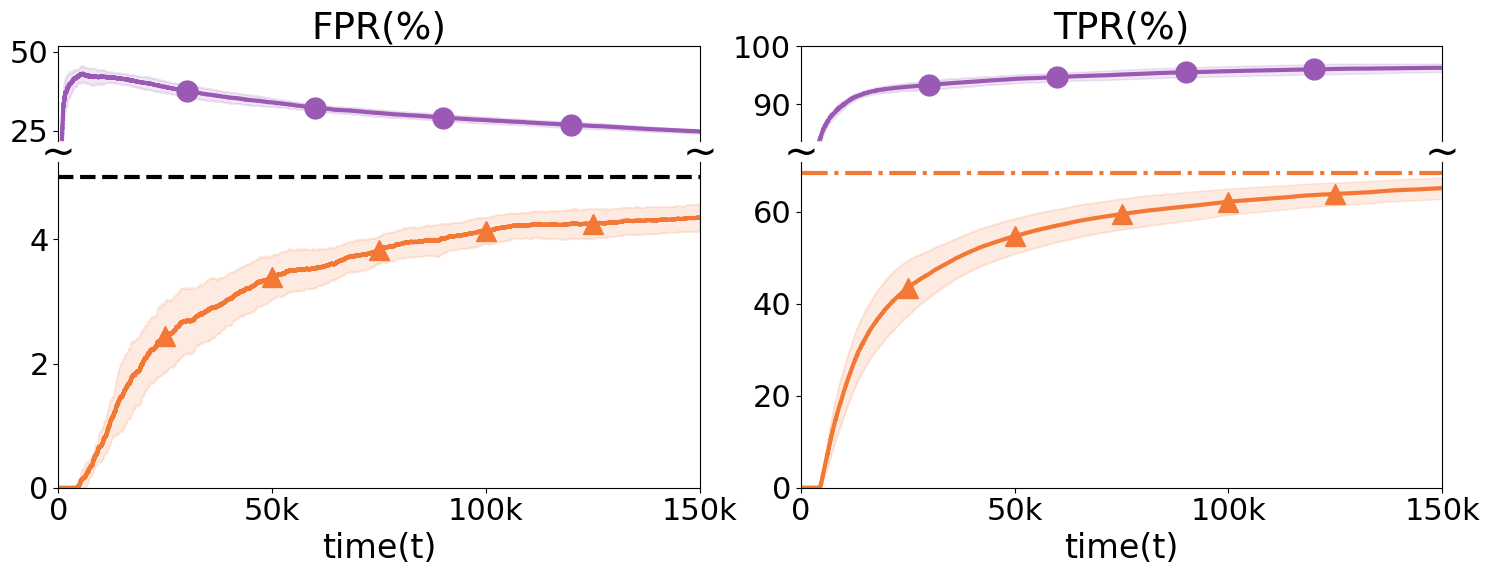
(a) Stationary, KNN, CIFAR-100 as OOD.

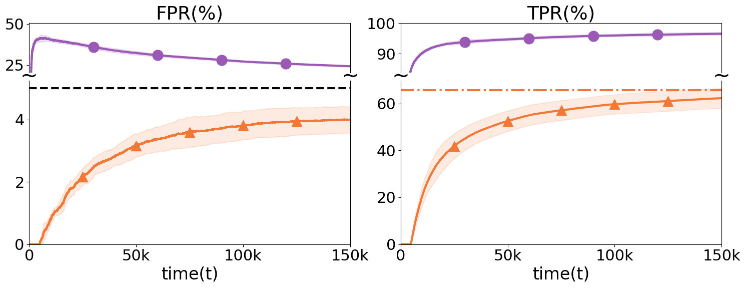
(b) Stationary, KNN, Near-OOD as OOD.

Figure 9: Comparison between ASAT and a naive binary classifier baseline. ASAT is initialized with KNN. CIFAR-10 as ID and CIFAR-100 and Near-OOD as OOD. Each method is repeated five times and is shown with mean and std. The binary classifier is trained using cross-entropy loss on the ID and OOD data collected up to time $t$, without importance sampling (since the classification is not based on score thresholding).

D.2 Searching for Constants in Heuristic LIL UCB

We derived the following theoretical LIL-based upper confidence bound (UCB) to ensure FPR control for ASAT with time-varying scoring functions $\widehat{g}_{t}$ for $t\geq 1$:

$$\psi_{t}(\delta):=\sqrt{\frac{3c_{t}}{N_{t}^{(o)}}\left[2\log\log\left(\frac{3c_{t}N_{t}^{(o)}}{2}\right)+\log\left(\frac{2U_{t}|\Lambda|}{\delta}\right)\right]},$$ (10)

where $U_{t}$ is the total number of scoring functions deployed in the system by time $t$. The inclusion of $U_{t}$ reflects the union bound required for FPR control given the time-varying scoring functions (see Appendix C). A similar UCB appears in the FSAT framework (Vishwakarma et al., 2024b), but without the $U_{t}$ term and with different definitions of $c_{t}$ and $N_{t}^{(o)}$. However, due to pessimistic constants in eq. (6) (e.g., $|\Lambda|$ may be large for small $\eta$), we define a heuristic UCB:

$$\psi^{H}_{t}(\delta):=c_{1}\sqrt{\frac{c_{t}}{N_{t}^{(o)}}\left[\log\log\left(c_{2}c_{t}N_{t}^{(o)}\right)+\log\left(\frac{c_{3}}{\delta}\right)\right]},$$

with constants $c_{1},c_{2},c_{3}$. In FSAT, $c_{1}=0.5$, $c_{2}=0.75$, and $c_{3}=1.0$ were chosen via simulation of a $p$-baised coin to keep failure probability under $5\%$. In the ASAT main experiments, where we fix the optimization frequencies, we retain $c_{2}$ and $c_{3}$ but increase $c_{1}$ to 0.65 to account for the effect of $U_{t}$. The choice of $c_{1}$ depends on the number of scoring function updates, which requires adjustment if the optimization frequency changes.

D.3 Choice of $\mathcal{G}$

Our ASAT framework is flexible in the choices of $\mathcal{G}$. In the main experiments, we use a class $\mathcal{G}_{1}$ of two-layer neural networks defined on top of the ResNet18 model (He et al., 2016). Let $z\vcentcolon=r(x)$ be the output feature from the penultimate layer of the Resnet18, denoted as $r$, for an image $x$. A network $g\in\mathcal{G}_{1}$ takes $z$ as input and outputs a score $s\in\mathcal{S}$:

$$\mathcal{G}_{1}:=\left\{g:g(x)\vcentcolon=\bm{W_{2}}\,\text{ReLU}\left(\bm{W_{1}}r(x)\right)\right\},$$

where $\bm{W_{1}},\bm{W_{2}}$ are learnable weight matrices of the two layers. The optimization procedures are detailed in the next section. This class of scoring functions leverages pre-extracted features for ID/OOD points and adapts the scoring functions from scratch to the specific OOD instances encountered by the system. This design is motivated by the observation that the backbone already performs heavy representation learning, and the 2-layer neural network as the scoring function only needs to learn a separation between ID and OOD samples, which makes the training computationally lightweight and scalable.

D.4 Searching for Hyper-parameters

Parameter	Values
optimizer	AdamW, SGD
learning rate for $g$	0.00001, 0.0001, 0.001, 0.01
learning rate for $\lambda$	0.0001, 0.001, 0.01, 0.1
weight decay rate for $g$	0.0001, 0.001, 0.01, 0.1, 0.0
weight decay rate for $\lambda$	0.0001, 0.001, 0.01, 0.1, 0.0
$\beta$ in (P2)	0.5, 0.75, 1.0, 1.25, 1.5, 1.75, 2.0
$\kappa$ for sigmoid smoothness	1, 10, 50, 100

Table 2: Lists of hyper-parameters we swept over to find the best combination for training $g\in\mathcal{G}_{1}$ and $\lambda\in\Lambda$ in optimization (P2).

We determine the hyperparameters and their values for the optimization problem in (P2) over $\mathcal{G}_{1}$ via grid search. First, we find the best-performing hyperparameter combination for training $g\in\mathcal{G}_{1}$ in offline settings using i.i.d OOD and ID datasets. Then, we extend these choices to the ASAT settings, where only dependent OOD datasets are available. We verify that the same hyperparameters perform well in online settings, made possible by importance sampling techniques that preserve accurate FPR estimation in (2).

Table 2 lists the hyperparameters and their values we explored. Specifically, we run experiments on every different combination of these lists of hyperparameters. We use the AdamW optimizer (Kingma and Ba, 2014), with learning rates of 0.0001 for $g$ and 0.01 for $\lambda$, and a weight decay rate of 0.001 for L1 regularization for both $g$ and $\lambda$. We also set $\beta=1.5$ and $\kappa=50$.

D.5 Effects of Different Updating Frequencies

We define the optimization frequencies $\omega^{(ood)}_{i}$ as the number of newly human-labeled OOD points required since the last update for the $(i+1)$th update of the scoring functions. In stationary settings, we fix $\omega^{(ood)}_{i}$ to be 100 for $i\in\{1,...,20\}$, 500 for $i\in\{21,40\}$, and 1000 thereafter for consistency. This approach enables more frequent updates early on, with the frequency gradually decreasing as scoring functions improve. In nonstationary settings, we set $\omega^{(ood)}_{i}$ uniformly to avoid excessively infrequent updates after a shift. Additionally, $\omega^{(ood)}_{i}$ influences the width of LIL-based UCB. More frequent updates result in larger $U_{t}$, leading to a wider UCB. Thus, $\omega^{(ood)}_{i}$ presents a trade-off between faster OOD adaptation and larger UCB. More frequent updates of the scoring functions could also impact time efficiency, as each update requires additional computational resources.

To illustrate this, we run additional experiments in stationary settings with four different choices for $\omega^{(ood)}_{i}$: 100, 500, 1000, and 2500 uniformly for all $i\geq 1$. We fix $c_{1}=0.50$ for $\psi_{t}^{H}(\delta)$ across all frequencies, knowing this value is not large enough to provide strict FPR guarantees. This ensures a fair comparison across different frequencies. The results, shown in Figure (10), confirm our hypotheses: more frequent updates lead to faster adaptations but also result in a larger UCB width. More frequent updates impact time efficiency, with rough averages from five runs showing increased time costs. However, they also lead to better TPR convergence, which requires further exploration. Further research on update frequencies is left for future work.

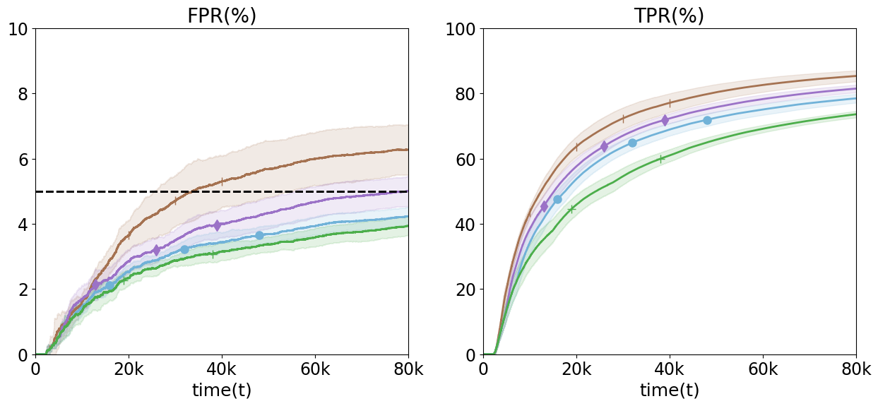
Figure 10: Results on the stationary setting with different update frequencies, with each method repeated 5 times (mean and std shown). CIFAR-10 as ID and Places365 as OOD. Optimization frequencies are set uniformly for 100, 500, 1000, and 2500 new OOD samples. We fix $c_{1}=0.5$ in the heuristic UCB $\psi_{t}^{H}(\delta)$.

D.6 Additional Experiments with Different Scoring Functions

In the main experiments, we present results for EBO and KNN. Additionally, we run additional experiments using the following alternative scoring functions, with the same settings and constants as in the main experiments. Note that while these scoring functions remain fixed in both FSFT and FSAT, the scoring function is immediately updated to a new scoring function from $\mathcal{G}_{1}$ in ASAT. We use these scoring functions adapted by Yang et al. (2022).

1. Energy Score (EBO). EBO (Liu et al., 2020) uses an energy function derived from a discriminative model to distinguish OOD inputs from ID data. Energy scores are shown to align more with probability density and to be less prone to overconfidence than softmax scores.

2. $K$-Nearest Neighbors (KNN). KNN (Sun et al., 2022) uses non-parametric nearest-neighbors distance without strong assumptions about the feature space. In particular, KNN measures the distance between an input and its $k$ closest ID neighbors. We use $k=50$ as in Open-OOD benchmarks.

3. Mahalanobis Distance (MDS). MDS (Lee et al., 2018b) computes the Mahalanobis distance between an input and the nearest class-conditional Gaussian distribution and outputs a confidence score based on Gaussian discriminant analysis (GDA).

4. Virtual Logits Matching (VIM). VIM (Wang et al., 2022) combines a class-agnostic score from the feature space with ID-dependent logits. It uses the residual of the feature against the principal space (we use dimension 10) and matches the logits with a constant scaling.

5. OOD in Neural Networks (ODIN). ODIN (Liang et al., 2018) uses softmax scores from DNNs, scales them with temperature, and applies gradient-based input perturbations to compute the score. We use a temperature of 1000 and a noise of 0.0014.

6. Activation Shaping (ASH). ASH (Djurisic et al., 2023) applies activation shaping, removing a large portion (e.g., 90%) of a sample’s activation at a late layer, simplifying the rest. The method requires no extra training or significant model modifications.

7. Simplified Hopfield Energy (SHE). SHE (Zhang et al., 2023) computes a score based on Hopfield energy in a store-and-compare paradigm. It transforms penultimate layer features into stored patterns representing ID data, which serve as anchors for scoring new inputs.

Results for stationary and nonstationary OOD settings are shown in Figures 11 and 12, respectively.

(a) MDS, CIFAR-10 as ID and CIFAR-100 as OOD.

(b) MDS, CIFAR-10 as ID and Near-OOD as OOD.

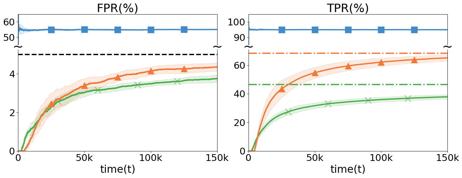
(c) VIM, CIFAR-10 as ID and CIFAR-100 as OOD.

(d) VIM, CIFAR-10 as ID and Near-OOD as OOD.

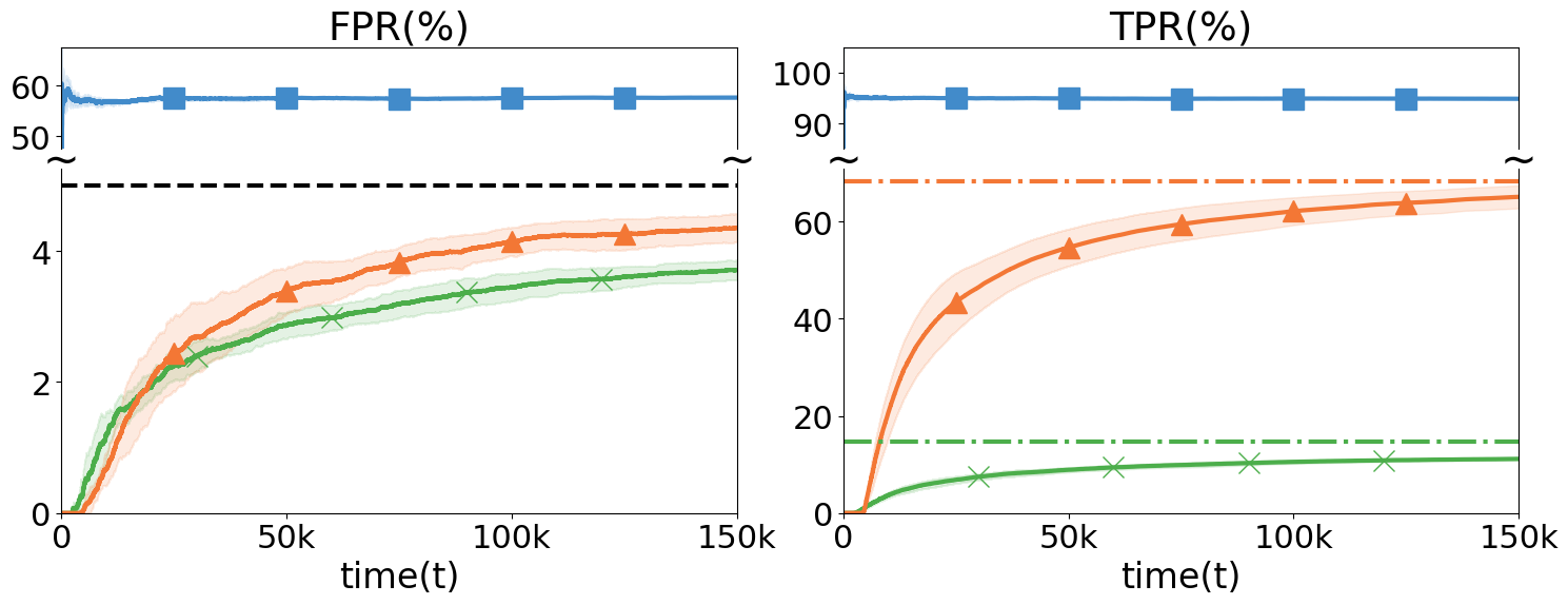
(e) ODIN, CIFAR-10 as ID and CIFAR-100 as OOD.

(f) ODIN, CIFAR-10 as ID and Near-OOD as OOD.

(g) ASH, CIFAR-10 as ID and CIFAR-100 as OOD.

(h) ASH, CIFAR-10 as ID and Near-OOD as OOD.

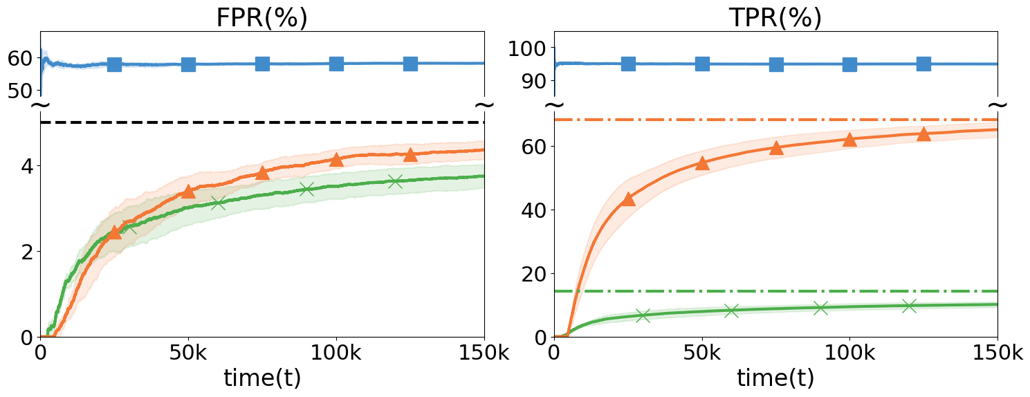
(i) SHE, CIFAR-10 as ID and CIFAR-100 as OOD.

(j) SHE, CIFAR-10 as ID and Near-OOD as OOD.

Figure 11: Results for stationary settings using CIFAR-10 as ID, with each method repeated 5 times (mean and std shown). Run with five additional scoring functions, MDS, VIM, ODIN, ASH, and SHE.

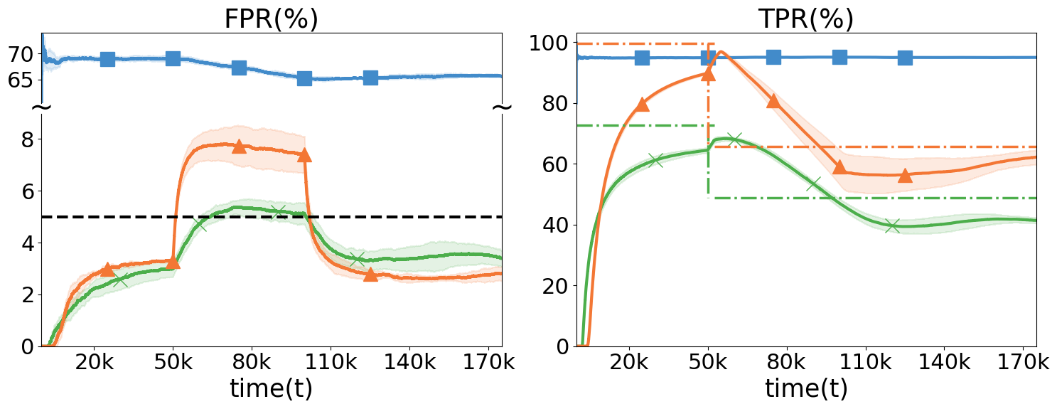
(a) MDS, CIFAR-10 as ID.

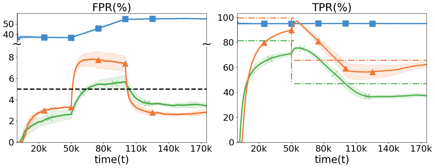
(b) VIM, CIFAR-10 as ID.

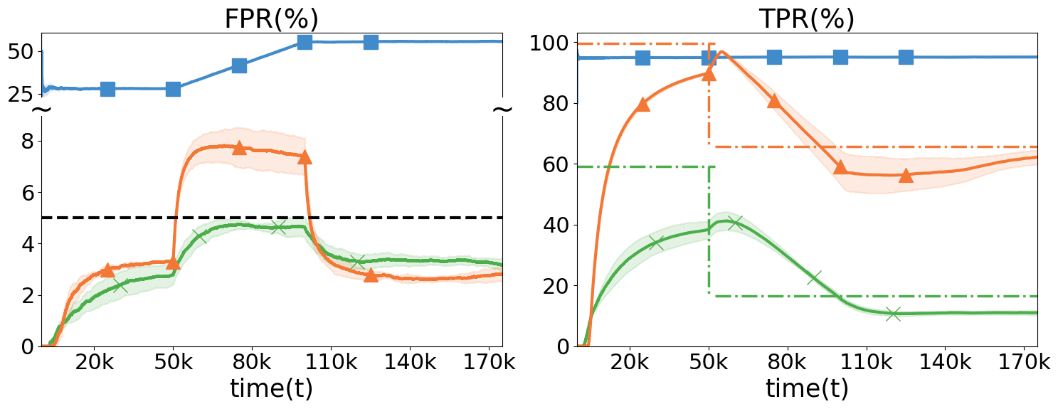
(c) ODIN, CIFAR-10 as ID.

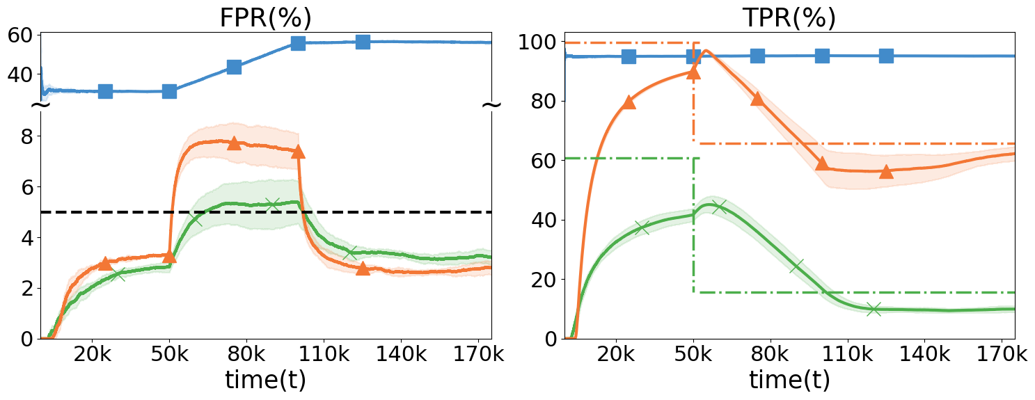
(d) SHE, CIFAR-10 as ID.

Figure 12: Results for nonstationary OOD settings using CIFAR-10 as ID, with each method repeated 5 times (mean and std shown). OOD distribution shifts from Far-OOD to Near-OOD. Run with four additional scoring functions, MDS, VIM, ODIN, and SHE.

D.7 Additional Experiments on Different ID Datasets

In the main experiments, we use CIFAR-10 as the ID dataset across all experiments. Additionally, we present results for CIFAR-100 (Deng et al., 2009) as the ID dataset. For stationary settings, we consider two OOD datasets: (i) CIFAR-10 and (ii) Places365. In the nonstationary OOD settings, we evaluate the scenario where a shift occurs at $t=50$k, transitioning from a Far-OOD mixture (MNIST, SVHN, and Texture) to a Near-OOD mixture (CIFAR-10, Tiny-ImageNet, and Places365). Results for stationary and distribution-shift settings are shown in Figures 13 and 14, respectively.

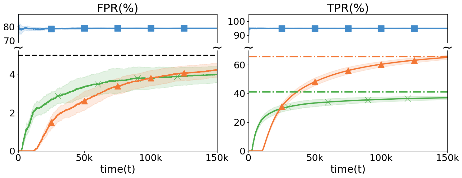
(a) EBO, CIFAR-100 as ID and CIFAR-10 as OOD.

(b) EBO, CIFAR-100 as ID and Near-OOD as OOD.

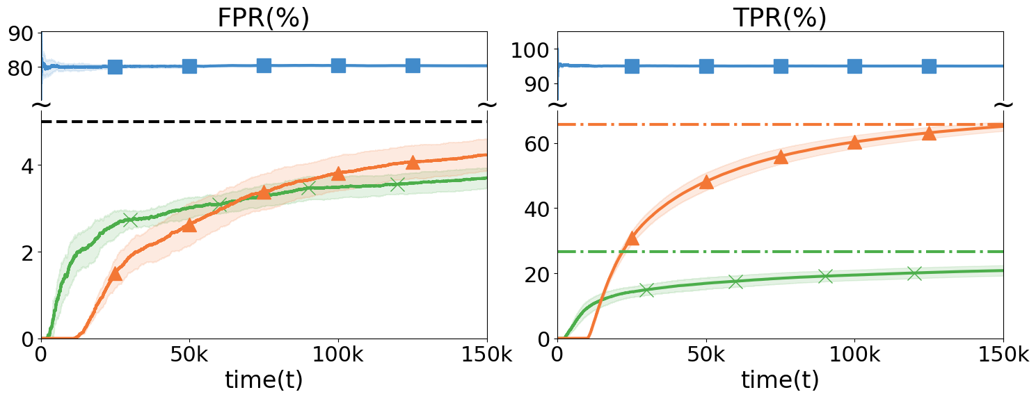
(c) KNN, CIFAR-100 as ID and CIFAR-10 as OOD.

(d) KNN, CIFAR-100 as ID and Near-OOD as OOD.

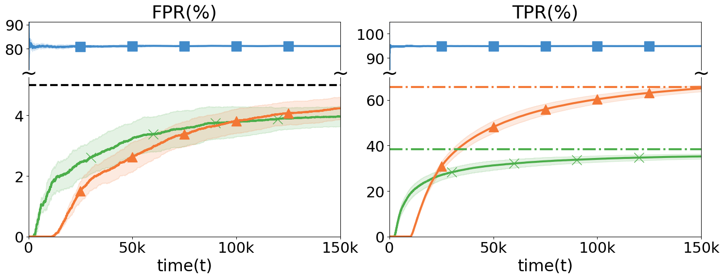
(e) ODIN, CIFAR-100 as ID and CIFAR-10 as OOD.

(f) ODIN, CIFAR-100 as ID and Near-OOD as OOD.

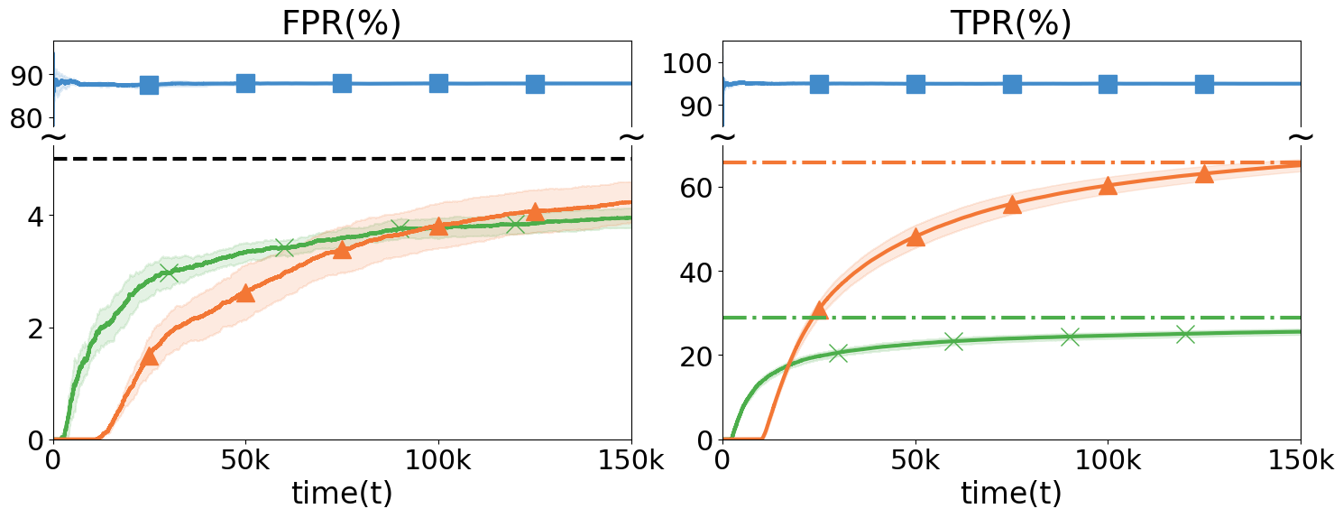
(g) ASH, CIFAR-100 as ID and CIFAR-10 as OOD.

(h) ASH, CIFAR-100 as ID and Near-OOD as OOD.

Figure 13: Results for stationary settings using CIFAR-100 as ID, with each method repeated 5 times (mean and std shown). Run with four scoring functions, EBO, KNN, VIM, and ODIN.

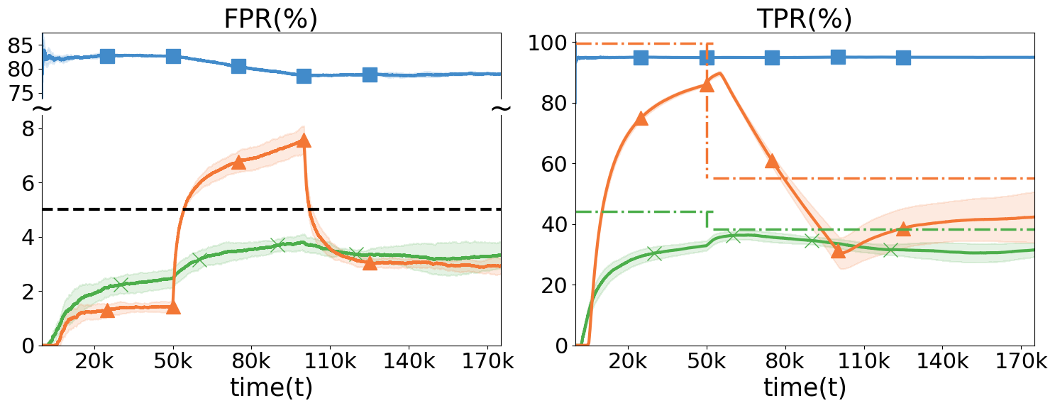
(a) EBO, CIFAR-100 as ID.

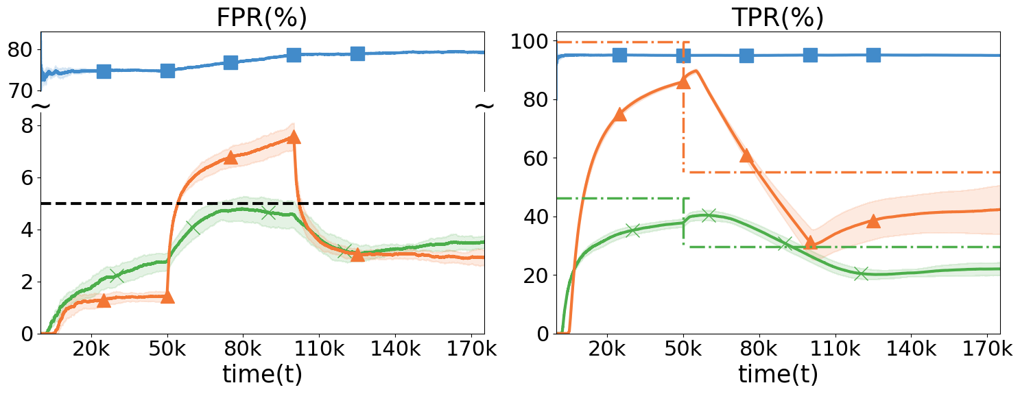
(b) KNN, CIFAR-100 as ID.

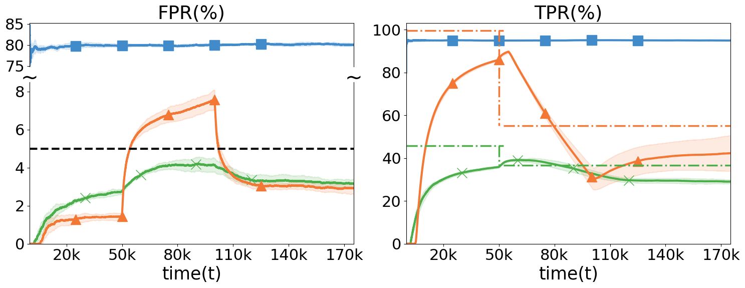
(c) ODIN, CIFAR-100 as ID.

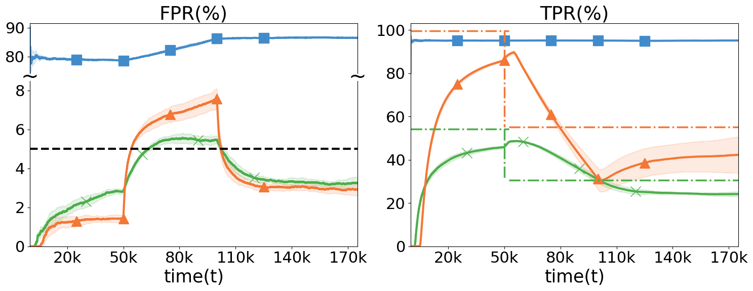
(d) VIM, CIFAR-100 as ID.

Figure 14: Results for nonstationary settings using CIFAR-100 as ID, with each method repeated 5 times (mean and std shown). OOD distribution shifts from Far-OOD to Near-OOD. Run with four additional scoring functions, MDS, VIM, ODIN, and SHE.

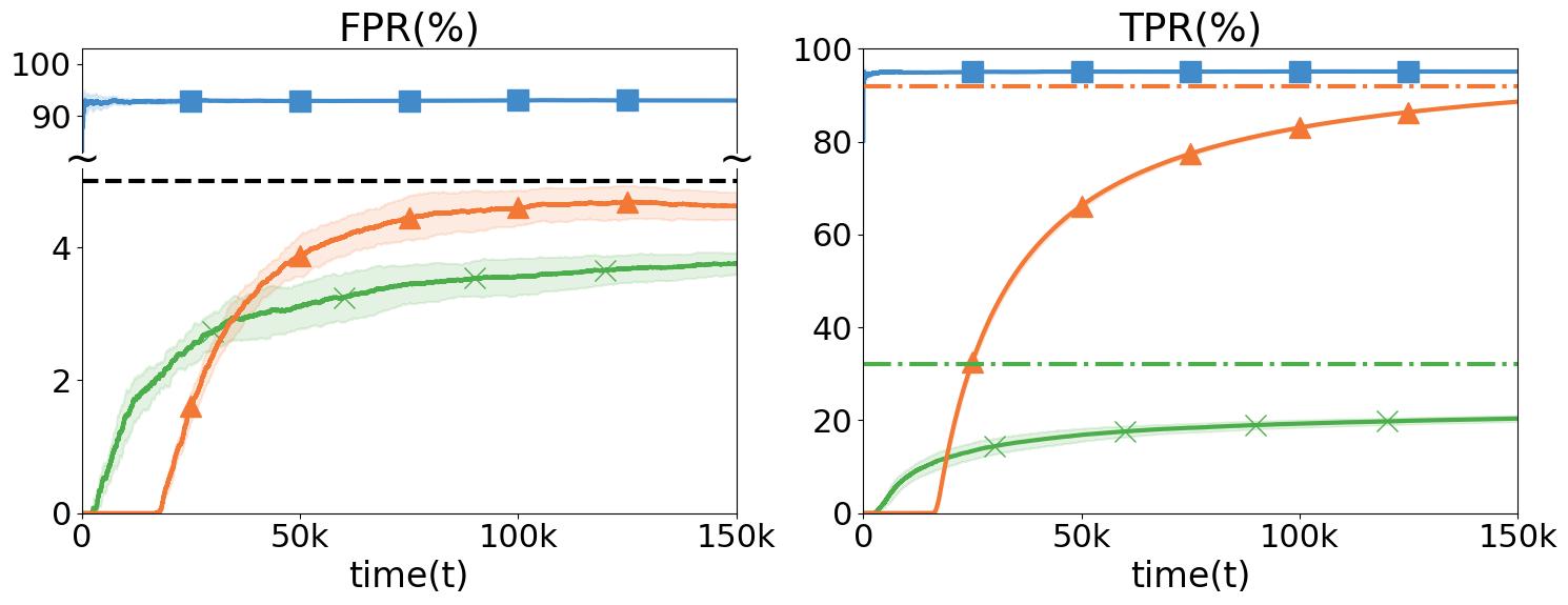
(a) Stationary, KNN, OpenImage-O as OOD.

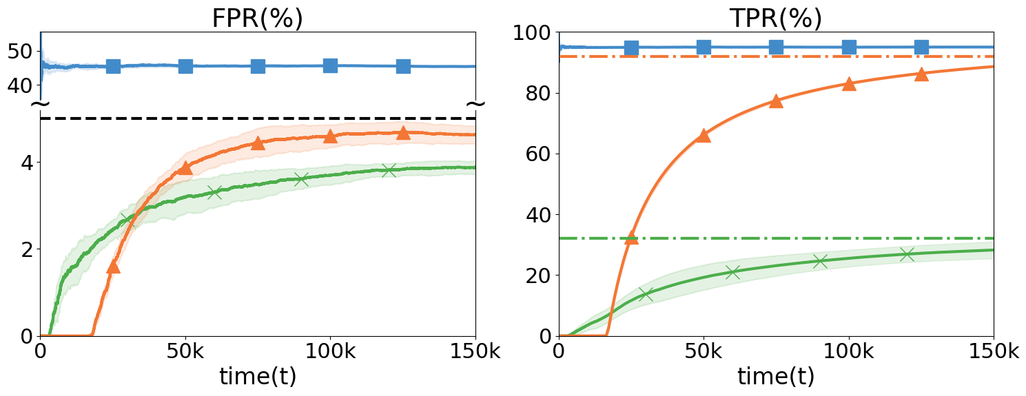
(b) Stationary, MDS, OpenImage-O as OOD.

Figure 15: Results on the stationary setting for ImageNet-1k as ID, with each method repeated 5 times (mean and std shown). KNN and MDS are the initial scoring functions and are fixed for FSFT and FSAT. The dotted-dash lines represent the expected TPR at FPR-5% for KNN, MDS, and $\widehat{g}^{\ast}$ (matching colors).

In addition, we have experiments in a large-scale setting using ViT-B/16 (Dosovitskiy et al., 2021) as the feature extractor and ImageNet-1k (Deng et al., 2009) as ID. In the stationary setting, we used OpenImage-O as OOD and compared ASAT against FSAT and FSFT with MSP and KNN scoring functions. As expected, ASAT outperformed FSAT in TPR while maintaining strict FPR control, which confirms that ASAT scales well to large datasets like ImageNet-1k and modern architectures like ViT. Results are shown in Figure 15.

References

- Amodei et al. (2016) D. Amodei, C. Olah, J. Steinhardt, P. F. Christiano, J. Schulman, and D. Mané. Concrete problems in AI safety. CoRR, abs/1606.06565, 2016.
- Bai et al. (2024) H. Bai, J. Zhang, and R. D. Nowak. AHA: Human-assisted out-of-distribution generalization and detection. In The Thirty-eighth Annual Conference on Neural Information Processing Systems, 2024.
- Balsubramani (2015) A. Balsubramani. Sharp finite-time iterated-logarithm martingale concentration. arXiv preprint arXiv:1405.2639, 2015.
- Bendale and Boult (2015) A. Bendale and T. E. Boult. Towards open set deep networks. 2016 IEEE Conference on Computer Vision and Pattern Recognition (CVPR), pages 1563–1572, 2015.
- Chen et al. (2021) G. Chen, P. Peng, X. Wang, and Y. Tian. Adversarial reciprocal points learning for open set recognition. IEEE Transactions on Pattern Analysis and Machine Intelligence, page 1–1, 2021. ISSN 1939-3539. doi: 10.1109/tpami.2021.3106743.
- Chen et al. (2023) Y. Chen, R. K. Vinayak, and B. Hassibi. Crowdsourced clustering via active querying: Practical algorithm with theoretical guarantees. In Proceedings of the AAAI Conference on Human Computation and Crowdsourcing, volume 11, pages 27–37, 2023.
- Darling and Robbins (1967) D. A. Darling and H. Robbins. Confidence sequences for mean, variance, and median. Proceedings of the National Academy of Sciences, 58(1):66–68, 1967.
- Deng et al. (2009) J. Deng, W. Dong, R. Socher, L.-J. Li, K. Li, and L. Fei-Fei. Imagenet: A large-scale hierarchical image database. In 2009 IEEE conference on computer vision and pattern recognition, pages 248–255. Ieee, 2009.
- Deng (2012) L. Deng. The mnist database of handwritten digit images for machine learning research [best of the web]. IEEE signal processing magazine, 29(6):141–142, 2012.
- DeVries and Taylor (2018) T. DeVries and G. W. Taylor. Learning confidence for out-of-distribution detection in neural networks. arXiv preprint arXiv:1802.04865, 2018.
- Djurisic et al. (2023) A. Djurisic, N. Bozanic, A. Ashok, and R. Liu. Extremely simple activation shaping for out-of-distribution detection. In The Eleventh International Conference on Learning Representations, 2023.
- Dosovitskiy et al. (2021) A. Dosovitskiy, L. Beyer, A. Kolesnikov, D. Weissenborn, X. Zhai, T. Unterthiner, M. Dehghani, M. Minderer, G. Heigold, S. Gelly, J. Uszkoreit, and N. Houlsby. An image is worth 16x16 words: Transformers for image recognition at scale. In International Conference on Learning Representations, 2021.
- He et al. (2016) K. He, X. Zhang, S. Ren, and J. Sun. Deep residual learning for image recognition. In Proceedings of the IEEE conference on computer vision and pattern recognition, pages 770–778, 2016.
- Heckel et al. (2019) R. Heckel, N. B. Shah, K. Ramchandran, and M. J. Wainwright. Active ranking from pairwise comparisons and when parametric assumptions do not help. The Annals of Statistics, 47(6):3099–3126, 2019.
- Hendrycks and Gimpel (2017) D. Hendrycks and K. Gimpel. A baseline for detecting misclassified and out-of-distribution examples in neural networks. In International Conference on Learning Representations, 2017.
- Howard and Ramdas (2022) S. R. Howard and A. Ramdas. Sequential estimation of quantiles with applications to A/B testing and best-arm identification. Bernoulli, 28(3):1704 – 1728, 2022. doi: 10.3150/21-BEJ1388.
- Huang and Li (2021) R. Huang and Y. Li. Mos: Towards scaling out-of-distribution detection for large semantic space. In Proceedings of the IEEE/CVF Conference on Computer Vision and Pattern Recognition, pages 8710–8719, 2021.
- Jamieson et al. (2014) K. Jamieson, M. Malloy, R. Nowak, and S. Bubeck. lil’ ucb : An optimal exploration algorithm for multi-armed bandits. In Proceedings of The 27th Conference on Learning Theory, volume 35, pages 423–439. PMLR, 2014.
- Jia and Grimmer (2022) Z. Jia and B. Grimmer. First-order methods for nonsmooth nonconvex functional constrained optimization with or without slater points. arXiv preprint arXiv:2212.00927, 2022.
- Katz-Samuels et al. (2022) J. Katz-Samuels, J. B. Nakhleh, R. D. Nowak, and Y. Li. Training ood detectors in their natural habitats. In International Conference on Machine Learning, 2022.
- Khinchine (1924) A. Khinchine. Über einen satz der wahrscheinlichkeitsrechnung. Fundamenta Mathematicae, 6:9–20, 1924.
- Kingma and Ba (2014) D. P. Kingma and J. Ba. Adam: A method for stochastic optimization. arXiv preprint arXiv:1412.6980, 2014.
- Kirichenko et al. (2020) P. Kirichenko, P. Izmailov, and A. G. Wilson. Why normalizing flows fail to detect out-of-distribution data. Advances in neural information processing systems, 33:20578–20589, 2020.
- Krizhevsky et al. (2009) A. Krizhevsky, G. Hinton, et al. Learning multiple layers of features from tiny images. Citeseer, 2009.
- Lai (1976) T. L. Lai. On Confidence Sequences. The Annals of Statistics, 4(2):265 – 280, 1976.
- Lee et al. (2018a) K. Lee, H. Lee, K. Lee, and J. Shin. Training confidence-calibrated classifiers for detecting out-of-distribution samples. In 6th International Conference on Learning Representations, ICLR 2018, 2018a.
- Lee et al. (2018b) K. Lee, K. Lee, H. Lee, and J. Shin. A simple unified framework for detecting out-of-distribution samples and adversarial attacks. Advances in neural information processing systems, 31, 2018b.
- Liang et al. (2018) S. Liang, Y. Li, and R. Srikant. Enhancing the reliability of out-of-distribution image detection in neural networks. In International Conference on Learning Representations, 2018.
- Liu et al. (2020) W. Liu, X. Wang, J. Owens, and Y. Li. Energy-based out-of-distribution detection. Advances in Neural Information Processing Systems, 33:21464–21475, 2020.
- Ming et al. (2023) Y. Ming, Y. Sun, O. Dia, and Y. Li. How to exploit hyperspherical embeddings for out-of-distribution detection? In The Eleventh International Conference on Learning Representations, 2023.
- Nadaraya (1965) E. A. Nadaraya. On non-parametric estimates of density functions and regression curves. Theory of Probability & Its Applications, 10(1):186–190, 1965. doi: 10.1137/1110024.
- Natarajan et al. (2013) N. Natarajan, I. S. Dhillon, P. K. Ravikumar, and A. Tewari. Learning with noisy labels. Advances in neural information processing systems, 26, 2013.
- Nguyen et al. (2015) A. M. Nguyen, J. Yosinski, and J. Clune. Deep neural networks are easily fooled: High confidence predictions for unrecognizable images. In CVPR, pages 427–436. IEEE Computer Society, 2015.
- Park and Van Hentenryck (2023) S. Park and P. Van Hentenryck. Self-supervised primal-dual learning for constrained optimization. In Proceedings of the AAAI Conference on Artificial Intelligence, volume 37, pages 4052–4060, 2023.
- Ren et al. (2019) J. Ren, P. J. Liu, E. Fertig, J. Snoek, R. Poplin, M. Depristo, J. Dillon, and B. Lakshminarayanan. Likelihood ratios for out-of-distribution detection. In Advances in Neural Information Processing Systems, volume 32, 2019.
- Salehi et al. (2022) M. Salehi, H. Mirzaei, D. Hendrycks, Y. Li, M. H. Rohban, and M. Sabokrou. A unified survey on anomaly, novelty, open-set, and out-of-distribution detection: Solutions and future challenges, 2022.
- Sehwag et al. (2021) V. Sehwag, M. Chiang, and P. Mittal. Ssd: A unified framework for self-supervised outlier detection. In International Conference on Learning Representations, 2021.
- Stutz et al. (2022) D. Stutz, K. D. Dvijotham, A. T. Cemgil, and A. Doucet. Learning optimal conformal classifiers. In International Conference on Learning Representations, 2022.
- Sun et al. (2022) Y. Sun, Y. Ming, X. Zhu, and Y. Li. Out-of-distribution detection with deep nearest neighbors. In International Conference on Machine Learning, pages 20827–20840. PMLR, 2022.
- Vinayak (2018) R. K. Vinayak. Graph Clustering: Algorithms, analysis and query design. California Institute of Technology, 2018.
- Vishwakarma et al. (2023) H. Vishwakarma, H. Lin, F. Sala, and R. Korlakai Vinayak. Promises and pitfalls of threshold-based auto-labeling. Advances in Neural Information Processing Systems, 36:51955–51990, 2023.
- Vishwakarma et al. (2024a) H. Vishwakarma, Y. Chen, S. S. S. N. GNVV, S. J. Tay, R. K. Vinayak, and F. Sala. Pablo: Improving semi-supervised learning with pseudolabeling optimization. In NeurIPS 2024 Workshop: Self-Supervised Learning-Theory and Practice, 2024a.
- Vishwakarma et al. (2024b) H. Vishwakarma, Y. Chen, S. J. Tay, S. S. S. Namburi, F. Sala, and R. Korlakai Vinayak. Pearls from pebbles: Improved confidence functions for auto-labeling. Advances in Neural Information Processing Systems, 37:15983–16015, 2024b.
- Vishwakarma et al. (2024c) H. Vishwakarma, H. Lin, and R. K. Vinayak. Taming false positives in out-of-distribution detection with human feedback. In International Conference on Artificial Intelligence and Statistics, pages 1486–1494. PMLR, 2024c.
- Wang et al. (2022) H. Wang, Z. Li, L. Feng, and W. Zhang. Vim: Out-of-distribution with virtual-logit matching. In Proceedings of the IEEE/CVF Conference on Computer Vision and Pattern Recognition, pages 4921–4930, 2022.
- Wei et al. (2022) H. Wei, R. Xie, H. Cheng, L. Feng, B. An, and Y. Li. Mitigating neural network overconfidence with logit normalization. International Conference on Learning Representations, 2022.
- Yang et al. (2022) J. Yang, P. Wang, D. Zou, Z. Zhou, K. Ding, W. Peng, H. Wang, G. Chen, B. Li, Y. Sun, et al. Openood: Benchmarking generalized out-of-distribution detection. Advances in Neural Information Processing Systems, 35:32598–32611, 2022.
- Yang et al. (2024) J. Yang, K. Zhou, Y. Li, and Z. Liu. Generalized out-of-distribution detection: A survey. International Journal of Computer Vision, 132(12):5635–5662, 2024.
- Zhang et al. (2023) J. Zhang, Q. Fu, X. Chen, L. Du, Z. Li, G. Wang, xiaoguang Liu, S. Han, and D. Zhang. Out-of-distribution detection based on in-distribution data patterns memorization with modern hopfield energy. In The Eleventh International Conference on Learning Representations, 2023.
- Zhou et al. (2017) B. Zhou, A. Lapedriza, A. Khosla, A. Oliva, and A. Torralba. Places: A 10 million image database for scene recognition. IEEE transactions on pattern analysis and machine intelligence, 40(6):1452–1464, 2017.