NMPCB: A Lightweight and Safety-Critical Motion Control Framework
Abstract
In multi-obstacle environments, real-time performance and safety in robot motion control have long been challenging issues, as conventional methods often struggle to balance the two. In this paper, we propose a novel motion control framework composed of a Neural network-based path planner and a Model Predictive Control (MPC) controller based on control Barrier function (NMPCB) . The planner predicts the next target point through a lightweight neural network and generates a reference trajectory for the controller. In the design of the controller, we introduce the dual problem of control barrier function (CBF) as the obstacle avoidance constraint, enabling it to ensure robot motion safety while significantly reducing computation time. The controller directly outputs control commands to the robot by tracking the reference trajectory. This framework achieves a balance between real-time performance and safety. We validate the feasibility of the framework through numerical simulations and real-world experiments.
I Introduction
In the design of robot motion planners and controllers, safety has always been the paramount requirement, considering the rapid development of robot systems[1]. The control method based on CBF has garnered significant attention for offering a simple yet safety-guaranteed approach to robot motion control[2]. In particular, the control method that integrates CBF and MPC have demonstrated superior performance in safety control by predicting future states [3]. However, this method often fails to obtain an optimal solution within a short time, especially for nonlinear kinematic systems where solution failure frequently occurs. Consequently, it also demands a high level of precision from the reference trajectory.
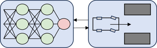
This letter presents a novel framework that integrates a neural network-based planner with an improved CBF-based MPC controller to ensure safety and real-time performance in robot motion control. The proposed framework serves both as a real-time local planner and as a controller.
I-A Related Work
I-A1 Path Planner
Sampling-based and search-based methods have been extensively studied, such as A*[4], PRM[5], and RRT[6]. These methods are fundamental in the field of robotics for path planning and have been widely researched and implemented in various applications. However, these methods often suffer from high computational costs and prolonged computation times, thus being only applicable to low-dimensional spaces.
Learning-based path planning methods are capable of rapidly generating high-quality paths, adapting to complex environments, and reducing reliance on prior knowledge[7][8]. For instance, neural A*[9], which is based on deep learning, offers a more efficient approach to path generation. However, since these methods can only plan paths offline, while the controllers can effectively track the paths, the prerequisite is the ability to adjust control inputs in real time. Optimization-based methods can achieve real-time path planning but often exhibit slower planning speeds[10][11].
I-A2 Optimization-Based Controller
Collision-free optimal control means finding the maximum or minimum value of the cost function under constraints. For instance, the TEB[12] algorithm achieves motion control by solving a multi-objective optimization problem. MPC has demonstrated significant potential in collision-free tasks[13].
The CBF serves as a safety boundary function for the control process, providing assurance of the robot’s safety[2][14]. CBF is particularly well-suited for collision avoidance constraints and have numerous applications in the fields of robotic manipulators [15] and vehicular systems [16]. In discrete-time systems, discrete-time control barrier function (DCBF) shows good performance in terms of safety constraints [17]. Research has been conducted on DCBF in the control and planning problems of multi-step optimization [18].
CBF-based MPC combines the advantages of both and has been increasingly used in recent years[19]. Similarly, DCBF can also be combined with MPC to achieve better results in obstacle avoidance problems [20]. The corresponding control method has been validated on both bipedal robots[21] and vehicle systems[22]. However, the above methods either oversimplify the control scenarios or have difficulty meeting the real-time requirements of control.
I-B Contributions
The contributions of this paper are as follows:
-
•
We propose an encoder-decoder path planning architecture which can determine the subsequent target point using historical path information and employs the Dubins curve to the target point as the reference path input to the control module.
-
•
Based on our planning architecture, we have improved the MPC-DCBF formulation to better accommodate nonlinear kinematic constraints and ensure its real-time performance.
-
•
We conducted numerical simulations and real-world experiments for the proposed framework in this letter, and performed comparative experiments with several baseline schemes.
I-C Paper Structure
The structure of this paper is organized as follows: In Section II, we present the preliminaries of MPC and CBF. In Section III, we introduce our proposed framework, along with the detailed design of the planner and controller. In Section IV, we describe our numerical simulations and real-world experiments. Finally, Section V concludes the paper.
II Preliminaries
In this section, we will introduce MPC and the optimization formulation using DCBF as the collision avoidance constraint.
II-A Model Predictive Control
The state transition equation of the robot is formulated as follows:
| (1) |
where and denote the state and control input of the robot at time step respectively, and is continuous.
If the distance to obstacles is employed as a collision avoidance constraint, then the MPC control formulation (MPC-DC) at time is given as follows:
| (2a) | ||||
| s.t. | ||||
| (2b) | ||||
| (2c) | ||||
| (2d) | ||||
| (2e) | ||||
Here, The functions and in (2a) represent the terminal cost and the cost associated with tracking the reference trajectory, respectively. Constraint (2d) indicates that the initial state of the robot is and the subsequent states are predicted via the system dynamics given in (2b), and constraint (2d) also specifies the terminal constraint. Both state and input constraints are provided by (2c). The collision avoidance constraint is given by (2e), which can be defined under various Euclidean norms.
We can also regard the MPC-DC as a path planning module. The path planning problem can be formulated as planning a collision-free trajectory for the robot from the initial state to the target state . If we set the value of in the optimization model (2) to 0 and solve for the optimal state , this becomes a standard path planning problem. We will employ an encoder-decoder model to address the path planning problem, the specifics of which will be discussed in Section III-A.
II-B Control Barrier Function
If the dynamical system (1) is safe with respect to the set , then any trajectory initiated from within will remain within . The set is defined as the 0-superlevel set of a continuous function as:
| (3) |
We refer to as the safety set, which encompasses all regions without obstacles. is defined as a DCBF, if satisfied
| (4) | ||||
Let . Satisfying (3) implies , that is, the lower bound of the DCBF decreases exponentially with the decay rate [18].
| (5) |
Then, if the initial state is within the safety set and , all subsequent states will also remain within the safety set , which implies that the resulting trajectory is safe.
The formulation proposed later in [nmpc dcbf 33] introduces a slack variable to balance feasibility and safety as follows:
| (6) |
The MPC control formulation based on DCBF constraints (MPC-DCBF) at time is presented as follows:
| (7a) | ||||
| s.t. | ||||
| (7b) | ||||
| (7c) | ||||
| (7d) | ||||
| (7e) | ||||
The optimization formulation (7) is fundamentally similar to the optimization formulation (2). In formulation (7), and are the joint input and relaxation variables, respectively. is the penalty function for the relaxation variable.
III NMPCB Motion Control Framework
In this section, we introduce the NMPCB framework, which consists mainly of two components: neural network-based path planner and the DCBF-based MPC controller.
III-A Neural Dubins Model
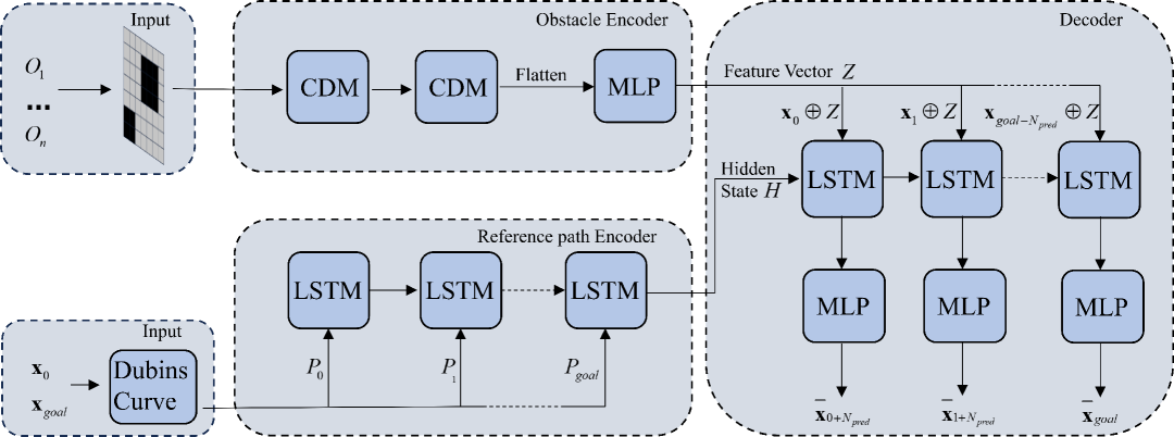
In this section, we describe our model formulation. As shown in Fig. 2 and Fig. 3, our model mainly consists of three components: the reference path encoder, the obstacle encoder, and the decoder.
The reference path encoder receives information from the start point and the goal point as input, where and represent the Cartesian coordinates, and denotes the heading angle. Within the model, a Dubins curve[23] is first generated from the to , and the coordinates of each point on the curve along are sequentially input into a single-layer LSTM module to obtain the hidden state . LSTM networks exhibit superior adaptability to motion continuity and enhanced robustness to noisy or irregular path data when processing path sequences.
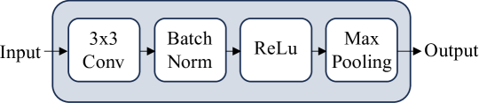
The obstacle encoder receives obstacle information as input. Each obstacle can be represented as , where and represent the center, and denotes the obstacle radius. The model maps the obstacle information onto a map matrix, where matrix values are set to at grid points with obstacles and at obstacle-free points, thus, the dimension of each map matrix is . This map matrix is then fed into a hierarchical feature extraction architecture comprising two convolutional downsampling modules (CDM) and a fully connected compression module, which ultimately outputs a low-dimensional feature vector . Each convolutional downsampling module comprises individual two-dimensional convolutional layers with a kernel size of . Each convolutional layer is connected with batch normalization (BN), an activation function, the rectified linear unit (ReLU), and a downsampling layer, max pooling, with filters of size .
Subsequently, the hidden state of the reference path encoder, the feature vector of the obstacle encoder, the endpoint , and all path points from the start point to the current point are input into the decoder. It then outputs the future states within a specified time horizon ,
| (8) |
The decoder network is composed of a single-layer LSTM network followed by a fully connected layer. We use a mean-squared-error (MSE) loss between the predicted state and the label next state during training, as follows:
| (9) |
Here, denotes the total number of planning steps.
After deriving the predicted state , a Dubins curve is constructed from the current point to to serve as a reference trajectory that is transmitted to the control module.
III-B Dual DCBF Constraint
To simplify the formulation of the obstacle avoidance problem, we introduce the following assumptions. First, the robot can be abstracted into a point mass model. Second, the geometry of any obstacle can be over-approximated with a union of convex polytopes, which is Defined as a bounded polyhedron. In the l-dimensional space, the -th obstacle can be described as:
| (10) |
where . represent the number of facets of polytopic sets for the -th obstacle.
Let the state of the robot be with its discrete-time dynamics as defined in (1) , represent the center of the robot. For , the computation of the squared minimum distance between the -th obstacle and the center can be be denoted by the function formula:
| (11a) | ||||
| (11b) | ||||
It can be noted that Equation (11) formulates a quadratic programming (QP) problem, thus representing a convex optimization problem. To ensure safety throughout the motion process, we apply the same DCBF constraint to each obstacle in relation to the robot. Thus, the safety set is defined as:
| (12) |
where denotes the closure of a set, and denotes the number of obstacles. Enforcing the DCBF constraint for each ensures that the state remains in .
We note that in the DCBF constraint (4), the computation of is required, which leads to the presence of non-differentiable implicit constraints in the optimization formulation and can consume significant computational time. Next, we introduce the dual DCBF constraints to address this issue.
For any convex optimization problem, a dual problem exists. The dual form of problem (11) is given by:
| (13a) | ||||
| s.t. | (13b) | |||
| (13c) | ||||
Here is the normal vector of the separating hyperplane.
According to the Weak Duality Theorem, for all optimization problems, it holds that for their respective dual problems. Since (11) is a convex optimization with linear constraint and has a well-defined optimum solution in , the Strong Duality Theorem[24] also holds, which states that
| (14) |
In accordance with the Strong Duality Theorem (14), we can substitute for the computation of , thereby circumventing the implicit dependence of on . We assume represents the cost associated with any feasible solution of (13). Since (13) is a maximization problem, we can derive the following inequality relationship:
| (15) |
Then, we can transform the DCBF constraints into a more stronger form:
| (16) |
This represents a stronger DCBF constraint that satisfies the (4). The substitution of the DCBF constraint with (16) requires satisfying (13b) and (13c), as follows:
| (17a) | |||
| (17b) | |||
According to the Strong Duality Theorem (14), satisfying (10b)-(10c) such that for all
| (18) |
This implies that if and only if satisfy (13), for all fixed , the input satisfies the DCBF constraint (5) with implicitly defined, which also implies that the set of feasible inputs does not diminish at any .
Similarly, we can apply the aforementioned method to optimization problem (11) to establish stronger DCBF constraints. Let be any feasible solution to (11). Since (11) is a minimization problem, we can derive the following inequality relationship:
| (19) |
Then we can enforce the stronger DCBF constrain:
| (20) |
Comparing with equation (4), we can observe the transformation of the DCBF constraints:
| (21) |
Integrating the analysis presented above, we define the dual DCBF constraints as follows:
| (22a) | |||
| (22b) | |||
| (22c) | |||
Introducing a slack variable has no effect on the aforementioned formulation.
III-C Optimization Formulation
We apply the dual DCBF constraints to the MPC algorithm as collision avoidance constraints to construct a multi-step optimization model, thereby providing enhanced assurance of safety in motion control. The optimization formulation for MPC-DUAL-DCBF (MDD) at time is presented as follows:
| (23a) | ||||
| s.t. | (23b) | |||
| (23c) | ||||
| (23d) | ||||
| (23e) | ||||
| (23f) | ||||
| (23g) | ||||
In the formulation, represents the optimal solution obtained by precomputing the minimum distance at time through (11). Constraint (23e) represents the dual DCBF constraint, while (23f)-(23g) denote the feasibility conditions of the dual DCBF constraint. The optimization formulation (23) illustrates only the dual DCBF constraint between obstacle and the region , however, during the motion control process, the corresponding dual DCBF constraints are applied to each pair of obstacles and the robot.
If the same dual DCBF constraints are imposed at each time step within a multi-step optimization model, it would result in a substantial computational burden. To reduce this complexity, we roll out the time and replace the RHS of each DCBF constraint with , as follows:
| (24) |
Replacing (23e) with Equation (24) can accelerate the computation. This modification affects neither the system feasibility nor its safety.
III-D Framework Overview
The framework consists of a planner and a controller. The planner utilizes Neural Dubins Model to determine the next target point and generates a Dubins curve from the current point to the target point, which serves as a reference trajectory and is passed to the control module. The control module solves equation (23) to output the optimal control commands, ensuring that the robot moves towards the goal without collisions.
We focus on the motion control problem of mobile robots, hence adopting the bicycle model as the kinematic model.The state vector of the robot is defined as , where and represent the coordinates of the rear axle center, is the velocity, and is the yaw angle. The control vector is defined as , where is the acceleration and is the steering angle of the front wheel. The kinematic equations are given by:
| (25a) | |||
| (25b) | |||
| (25c) | |||
| (25d) | |||
where represents the time step and denotes the wheelbase.
The cost function (23a) is composed of terminal cost, stage cost, and slack function cost, respectively as
| (26a) | ||||
| (26b) | ||||
| (26c) | ||||
where represents the reference trajectory. The stage cost consists of the tracking cost of the reference trajectory, the control effort cost, and the control smoothness cost.
For the point mass model of the robotic, we can ensure effective obstacle avoidance by setting a safety distance , which also alleviates the issue of decreased solution speed due to the incorporation of distant obstacles in the optimization problem.
For optimization problem (23), the geometric representation of the robot and obstacles can be altered to accommodate various scenarios. In scenarios where high solution speed is required and accurate shape information of obstacles can be obtained, an optimization formulation corresponding to a point mass robot model and convex polygon obstacles can be utilized (MDD-I). In scenarios where solution speed is not a critical factor and navigating through tight spaces is challenging, an optimization model that corresponds to a convex polygonal robot model and convex polygonal obstacles can be applied (MDD-II, [20]).
In the following section, we will conduct comparative experiments of the aforementioned algorithms across various scenarios.
IV Experiments and Results
In this section, we conduct numerical simulations of the NMPCB framework and perform ablation experiments to verify that both the planner and the controller significantly enhance the motion control problem. Furthermore, we have conducted real-world experiments with the proposed framework to validate its performance in actual environments.

IV-A Datasets Construction
Due to the scarcity of high-quality path planning datasets for deep learning in unstructured environments, we have constructed a dataset that includes information on obstacles and the robot’s motion trajectories. The generation of motion trajectories within the dataset is facilitated by the RDA [11] algorithm. We generated a substantial amount of motion trajectory data in unstructured scenarios by randomly creating obstacles and assigning start and end points within a certain range.
For ease of representation, obstacles are uniformly modeled as circles, with their information consisting of the center and radius of the circles. Trajectory information includes the coordinates of the robot’s rear axle center and the robot’s heading angle. We have excluded data where collisions occurred during motion, resulting in trajectory lengths shorter than a predetermined threshold.
We have generated a total of 12,000 instances for the training set and 3,000 instances for the test set.
IV-B Numerical Simulation
We have prepared the following four combinations of motion control algorithms for comparative experiments: (1) A Dubins curve connecting the starting point to the goal point is utilized as the planner, with the MPC-DCBF serving as the controller. (2) A Dubins curve connecting the starting point to the goal point is utilized as the planner, with the MDD-I serving as the controller. (3) The Neural Dubins Model is utilized as the planner, with the MDD-I serving as the controller. (4) The Neural Dubins Model is utilized as the planner, with the MDD-III serving as the controller. We have set the parameters for the aforementioned algorithms to , , and . The optimization problems are implemented in Python using CasADi[25] as the modeling language and solved with IPOPT [26] on Ubuntu 18.04.
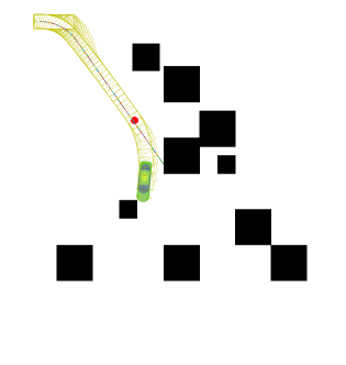
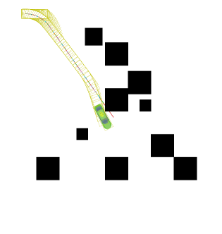
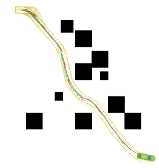
We validated our proposed framework in intelligent robot simulator (ir-sim)111https://github.com/hanruihua/ir_sim, which is a Python-based simulator for robotic algorithm development. We represent obstacles with black cubes, denote the area traversed by the robot with a yellow border, and illustrate the reference trajectory provided by the planner to the controller with colored lines.
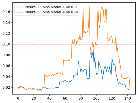
In Fig. 4LABEL:sub@fig4a, the red dots indicate points where the solver failed to find a solution, demonstrating the poor performance of MPC-DCBF in complex scenarios. Fig. 4LABEL:sub@fig4b shows that MDD-I can adapt to complex environments, however, due to the Dubins curve not accounting for obstacles, the controller collided while following the reference trajectory. Fig. 4LABEL:sub@fig4c - 4LABEL:sub@fig4d illustrate that, upon employing the Neural Dubins Model, all two algorithms are capable of planning a suitable collision-free trajectory. This demonstrates that the Neural Dubins Model provides an appropriate reference path. However, there is a significant difference in computation time among the two algorithms, especially in densely obstacle-populated areas, where the computation time for MDD-II often reaches around 0.15 seconds, whereas the computation time for MDD-I does not exceed 0.1 seconds. Fig. 5 reflects the disparity in their computation times.
To better compare the differences in success rate and average solution time among the two algorithms, we conducted comparative experiments across 50 randomly generated scenarios, and the results are presented in Table 1.
| Success Rate |
|
|
|||||
|
0.86 | Four | 0.172 | ||||
|
0.82 | Four | 0.851 |
Here, the success rate refers to the ratio of the number of scenarios where the robot successfully reaches the destination without collision to the total number of scenarios. The average solving time is the average single-step solving time in successful scenarios. The average maximum solving time refers to the average of the maximum single-step solving time in each successful scenario.
It can be observed that MDD-I and MDD-II exhibit similar success rates. However, both average solving time and average maximum solving time for MDD-I are significantly lower than those for MDD-II.
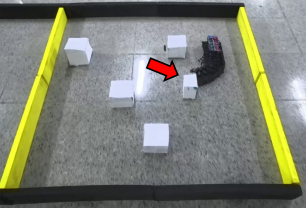
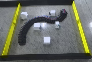
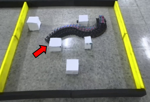
IV-C Real-World Experiments
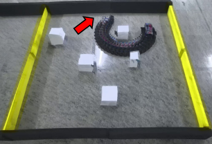
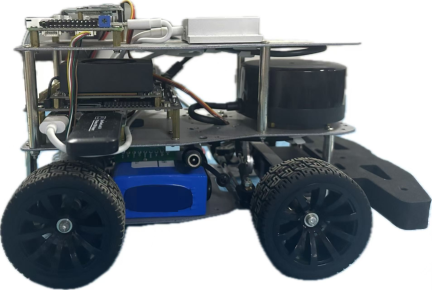
To validate the practical performance of the NMPCB framework in real-world scenarios, experiments were conducted on the robot depicted in Fig. 7. This robot is equipped with four wheels and employs Ackermann steering. Its sensor suite comprises a 2D LiDAR, an IMU, and wheel odometry. We utilized an NVIDIA Jetson Nano as the computing platform.
Utilizing the aforementioned hardware, we conducted comparative experiments of the four algorithms from numerical simulations in real-world settings. In Fig. 6LABEL:sub@fig6a, the MPC-DCBF algorithm faced persistent solution failures in the presence of multiple obstacles, ultimately resulting in a collision. In Fig. 6LABEL:sub@fig6b, although no solution failures occurred, collisions still took place due to the use of the Dubins curve as the reference trajectory. Comparing Fig. 6LABEL:sub@fig6c and Fig. 6LABEL:sub@fig6d, the MDD-II algorithm resulted in a collision due to the robot’s control module frequency exceeding the solution frequency of MDD-II. However, the MDD-I algorithm demonstrated superior real-time performance, successfully reaching the destination.
V CONCLUSIONS
In this paper, we propose NMPCB, a motion control framework that integrates neural networks with optimal control. This framework serves dual purposes as both a local planner and a controller. While ensuring the safety of the robot’s motion, it also demonstrates commendable real-time performance compared to other methods. For future research, we will optimize the Neural Dubins Model to enhance its capabilities in path planning. Additionally, we will focus on constructing optimization formulations of different forms to accelerate the solution process.
References
- [1] W. Ding, L. Zhang, J. Chen, and S. Shen, “Epsilon: An efficient planning system for automated vehicles in highly interactive environments,” IEEE Transactions on Robotics, vol. 38, no. 2, pp. 1118–1138, 2021.
- [2] A. D. Ames, S. Coogan, M. Egerstedt, G. Notomista, K. Sreenath, and P. Tabuada, “Control barrier functions: Theory and applications,” in 2019 18th European control conference (ECC). Ieee, 2019, pp. 3420–3431.
- [3] J. Zeng, B. Zhang, and K. Sreenath, “Safety-critical model predictive control with discrete-time control barrier function,” in 2021 American Control Conference (ACC). IEEE, 2021, pp. 3882–3889.
- [4] F. Duchoň, A. Babinec, M. Kajan, P. Beňo, M. Florek, T. Fico, and L. Jurišica, “Path planning with modified a star algorithm for a mobile robot,” Procedia engineering, vol. 96, pp. 59–69, 2014.
- [5] R. Bohlin and L. E. Kavraki, “Path planning using lazy prm,” in Proceedings 2000 ICRA. Millennium conference. IEEE international conference on robotics and automation. Symposia proceedings (Cat. No. 00CH37065), vol. 1. IEEE, 2000, pp. 521–528.
- [6] R. R. Radaelli, C. Badue, M. A. Gonçalves, T. Oliveira-Santos, and A. F. De Souza, “A motion planner for car-like robots based on rapidly-exploring random trees,” in Advances in Artificial Intelligence–IBERAMIA 2014: 14th Ibero-American Conference on AI, Santiago de Chile, Chile, November 24-27, 2014, Proceedings 14. Springer, 2014, pp. 469–480.
- [7] J. Wang, W. Chi, C. Li, C. Wang, and M. Q.-H. Meng, “Neural rrt*: Learning-based optimal path planning,” IEEE Transactions on Automation Science and Engineering, vol. 17, no. 4, pp. 1748–1758, 2020.
- [8] F. Meng, L. Chen, H. Ma, J. Wang, and M. Q.-H. Meng, “Nr-rrt: Neural risk-aware near-optimal path planning in uncertain nonconvex environments,” IEEE Transactions on Automation Science and Engineering, vol. 21, no. 1, pp. 135–146, 2022.
- [9] R. Yonetani, T. Taniai, M. Barekatain, M. Nishimura, and A. Kanezaki, “Path planning using neural a* search,” in International conference on machine learning. PMLR, 2021, pp. 12 029–12 039.
- [10] X. Zhang, A. Liniger, and F. Borrelli, “Optimization-based collision avoidance,” IEEE Transactions on Control Systems Technology, vol. 29, no. 3, pp. 972–983, 2020.
- [11] R. Han, S. Wang, S. Wang, Z. Zhang, Q. Zhang, Y. C. Eldar, Q. Hao, and J. Pan, “Rda: An accelerated collision free motion planner for autonomous navigation in cluttered environments,” IEEE Robotics and Automation Letters, vol. 8, no. 3, pp. 1715–1722, 2023.
- [12] C. Rösmann, F. Hoffmann, and T. Bertram, “Kinodynamic trajectory optimization and control for car-like robots,” in 2017 IEEE/RSJ International Conference on Intelligent Robots and Systems (IROS). IEEE, 2017, pp. 5681–5686.
- [13] J. Funke, M. Brown, S. M. Erlien, and J. C. Gerdes, “Collision avoidance and stabilization for autonomous vehicles in emergency scenarios,” IEEE Transactions on Control Systems Technology, vol. 25, no. 4, pp. 1204–1216, 2016.
- [14] H. Ma, J. Chen, S. Eben, Z. Lin, Y. Guan, Y. Ren, and S. Zheng, “Model-based constrained reinforcement learning using generalized control barrier function,” in 2021 IEEE/RSJ International Conference on Intelligent Robots and Systems (IROS). IEEE, 2021, pp. 4552–4559.
- [15] B. Dai, R. Khorrambakht, P. Krishnamurthy, V. Gonçalves, A. Tzes, and F. Khorrami, “Safe navigation and obstacle avoidance using differentiable optimization based control barrier functions,” IEEE Robotics and Automation Letters, vol. 8, no. 9, pp. 5376–5383, 2023.
- [16] J. Seo, J. Lee, E. Baek, R. Horowitz, and J. Choi, “Safety-critical control with nonaffine control inputs via a relaxed control barrier function for an autonomous vehicle,” IEEE Robotics and Automation Letters, vol. 7, no. 2, pp. 1944–1951, 2022.
- [17] A. Agrawal and K. Sreenath, “Discrete control barrier functions for safety-critical control of discrete systems with application to bipedal robot navigation.” in Robotics: Science and Systems, vol. 13. Cambridge, MA, USA, 2017, pp. 1–10.
- [18] J. Zeng, Z. Li, and K. Sreenath, “Enhancing feasibility and safety of nonlinear model predictive control with discrete-time control barrier functions,” in 2021 60th IEEE Conference on Decision and Control (CDC). IEEE, 2021, pp. 6137–6144.
- [19] Z. Jian, Z. Yan, X. Lei, Z. Lu, B. Lan, X. Wang, and B. Liang, “Dynamic control barrier function-based model predictive control to safety-critical obstacle-avoidance of mobile robot,” in 2023 IEEE International Conference on Robotics and Automation (ICRA). Ieee, 2023, pp. 3679–3685.
- [20] A. Thirugnanam, J. Zeng, and K. Sreenath, “Safety-critical control and planning for obstacle avoidance between polytopes with control barrier functions,” in 2022 International Conference on Robotics and Automation (ICRA). IEEE, 2022, pp. 286–292.
- [21] S. Teng, Y. Gong, J. W. Grizzle, and M. Ghaffari, “Toward safety-aware informative motion planning for legged robots,” arXiv preprint arXiv:2103.14252, 2021.
- [22] H. Ma, J. Chen, S. Eben, Z. Lin, Y. Guan, Y. Ren, and S. Zheng, “Model-based constrained reinforcement learning using generalized control barrier function,” in 2021 IEEE/RSJ International Conference on Intelligent Robots and Systems (IROS). IEEE, 2021, pp. 4552–4559.
- [23] A. M. Shkel and V. Lumelsky, “Classification of the dubins set,” Robotics and Autonomous Systems, vol. 34, no. 4, pp. 179–202, 2001.
- [24] S. P. Boyd and L. Vandenberghe, Convex optimization. Cambridge university press, 2004.
- [25] J. A. Andersson, J. Gillis, G. Horn, J. B. Rawlings, and M. Diehl, “Casadi: a software framework for nonlinear optimization and optimal control,” Mathematical Programming Computation, vol. 11, pp. 1–36, 2019.
- [26] L. T. Biegler and V. M. Zavala, “Large-scale nonlinear programming using ipopt: An integrating framework for enterprise-wide dynamic optimization,” Computers & Chemical Engineering, vol. 33, no. 3, pp. 575–582, 2009.