A dynamic view of the double descent
Abstract.
It has been observed by Belkin et al. that overparametrized neural networks exhibit a ‘double descent’ phenomenon. That is, as the model complexity, as reflected in the number of features, increases, the training error initially decreases, then increases, and then decreases again. A counterpart of this phenomenon in the time domain has been noted in the context of epoch-wise training, viz., that the training error decreases with time, then increases, then decreases again. This note presents a plausible explanation for this phenomenon by using the theory of two time scale stochastic approximation and singularly perturbed differential equations, applied to the continuous time limit of the gradient dynamics. This adds a ‘dynamic’ angle to an already well studied theme.
Key words: stochastic gradient descent; double descent; overparametrized neural networks; stochastic approximation; singularly perturbed differential equations; two time scales
1. Introduction
Beginning with Belkin et al. [6], the phenomenon of ‘double descent’ in the training of overparametrized neural networks using stochastic gradient descent (SGD) has been flagged and extensively studied from various angles [1, 5, 7, 11, 13, 17, 20, 21, 23, 28]. See also some generalizations such as [5, 13]. (See [22] for some pre-history.) The most common formulation has been in terms of increasing model complexity as reflected in an increasing basket of features. Simply put, the training error for SGD applied to this problem first decreases as new features are added, then increases, then decreases again.
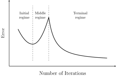
The aim of this note is to consider an alternative paradigm for double descent based on the dynamics of the corresponding SGD as time progresses. This has already been introduced in the context of epoch-wise gradient descent [14, 18, 25, 26, 27, 29]. The novelty in this work is that we view the iterates as a two time scale stochastic approximation. Specifically, it considers the loss as a function of the number of iterates of the SGD, equivalently, the number of training samples. The structure of the loss function is exploited to justify the time scale separation. This in turn leads to two clearly defined regimes wherein one expects descent due to distinct mechanisms and on different time scales. That leaves an in-between regime where the time scales cannot be separated, which is typically not analyzed in the traditional asymptotic analysis. It is argued that this is the regime when the ascent takes place. Some of the aforementioned works already have similar ideas. Our aim here is to give what we believe is to be the correct mathematical formulation in the framework of stochastic approximation. See Fig. 1 for a schematic.
The two time scale dynamics is derived in the next section, following which we recall the basics of two time scale stochastic approximation in Section 3. This framework is then used in Section 4 to identify three ‘regimes’ for SGD with a constant stepsize in an overparametrized framework, leading to an explanation of the double descent phenomenon. This is done assuming unique minimizers wherever the minimization operation occurs. Section 5 outlines in broad terms a picture for the general case where this assumption is relaxed. The final section concludes with brief comments.
We shall denote by the vector of all zeros, of appropriate dimension depending on the context. We abbreviate ‘ordinary differential equation’ as ‘ODE’.
2. Preliminaries
Our starting point is the oft observed fact that functions of a large number of variables typically depend predominantly on a significantly smaller number of variables. In fact, some rigorous statements along these lines are possible when a Lipschitz condition or a bound on the modulus of continuity is imposed on the function [2].
Consider a function for some , which will serve as our surrogate for the input-output map of an overparametrized neural network. Since our interest is in analyzing stochastic gradient descent (SGD) for this function, we shall assume that it is continuously differentiable. Furthermore, we assume that is of the form
| (2.1) |
for some with , , and . Then depends only weakly on the variable .
Note that in reality the separation of scales of dependence may not be binary as depicted here. There may be multiple, even a continuum of degrees of dependence. Our aim is only to formulate a stylized model that presents a simple scenario wherein the temporal double dip can be explained.
Nor do we assign the three regimes we identify relative importances in the overall scheme, as this can depend on the specifics of the problem. For example, if only the strongly dependent variables matter, then only the first descent is important and one might consider ‘early stopping’ as in [25]. We do not get into these issues here.
We begin with the derivation of the two time scale SGD model. Let (resp., ) denote the gradient (resp., partial gradient) with respect to the variable (resp., variables ). These are viewed as column vectors. Then we have
The SGD iteration for with a small constant stepsize is given by
Here is the standard ‘martingale difference noise’, i.e., a sequence of integrable random variables in satisfying
where the -field for . Partition as for , where denote resp. the first and the last components of . Letting , this iteration can be rewritten as the coupled iteration
| (2.2) | |||||
| (2.3) |
Since , this is recognized as a constant stepsize counterpart of two time scale stochastic approximation introduced in [9] for decreasing stepsizes, see Section 9.4, bullet 4, of [10].
3. Two time scale iterations
The above observation facilitates analysis of the SGD in (2.2)-(2.3) as a two time scale stochastic approximation, with the difference (as opposed to [9]) being that we have constant stepsizes . In the classical theory of [9], are replaced by decreasing stepsizes satisfying the Robbins-Monro conditions and , along with the additional condition as . As argued in [9] (also [10], Section 8.1), this ensures the separation of time scales of (2.2) and (2.3). One can then rigorously argue that the iterates track the asymptotic behaviour of the ODE
| (3.1) |
for a slowly varying . Suppose that for each , has a unique minimum that is Lipschitz in . Then as argued in ibid., a.s. Suppose, as in ibid., that the ODE
| (3.2) |
has a unique globally asymptotically stable equilibrium . Then it is shown in ibid. that track the asymptotic behaviour of the ODE
| (3.3) |
and
| (3.4) |
Remark 3.1.
In [9], [10], a more general two time scale dynamics is considered, the driving vector fields on both time scales are not necessarily negative gradients. We have specialized the results therein to the case where on both time scales, it is a gradient descent in the appropriate variable. Thus the above statements represent the claims from [9], [10] specialized to the present scenario.
The problem of proving that (3.2) converges can be handled as follows. Note that
by the envelope theorem, also known as Danskin’s theorem [12]. (See [16] or [4], pp. 42-46 for a modern treatment.) Thus (3.2) is also a gradient descent and will converge to the unique minimum in view of our assumptions. We state this as a lemma.
Lemma 3.2.
As , the unique minimum of .
We shall now use the corresponding results for two timescale stochastic approximation with constant step sizes, where one can only expect concentration near the desired limit and not a.s. convergence to it. This is captured by the results of [10], Section 9.4, bullet 4. In our context, they translate into the following.
Theorem 3.3.
For as above,
See ibid. for details.
4. The ‘double descent’
This classical asymptotic analysis does not explain the double descent. For that, we have to dig into the temporal behaviour of the SGD in greater detail, by identifying different regimes in its evolution. We do this next.
-
(1)
The initial regime: In the initial phase of the iterations, we expect the partial gradient and to be comparable and non-negligible, both being away from the corresponding componentwise minimum. The stepsizes are constant at . Thus the first part of the two time scale logic described above indicates that will hardly change whereas will quickly start approaching . This is the first descent.
-
(2)
The terminal regime: In the third and final phase, and hence . But remains significant. Hence will perform the SGD on
so as to approach . The will correspondingly approach . This is the second and final descent.
-
(3)
The ‘middle’ regime: This leaves the in-between regime when the partial gradients and are of comparable magnitude and the time scales of descents in the and variables cannot be separated. This is a non-asymptotic and hence commonly ignored regime in the theory of two time scale stochastic approximation. As towards the end of the initial regime, one may expect that , so is small. On the other hand, is not small, but , because of which and can have comparable sizes. Consequently the asymptotic analysis of the preceding section based on the separation of time scales does not apply. In fact, the approximation itself is based on viewing as changing slowly relative to , which is no longer valid - they can change at comparable rates. In other words, slowing down of (2.2) due to near-convergence has made the ‘quasi-static’ assumption on invalid and the ensuing lack of complete convergence of to has made the validity of (3.3) questionable. In this transition regime between the two regimes (resp. the initial and terminal regimes above) that are captured by the two time scale analysis, it is a classical SGD in a pinched landscape, the simplest prototype of which is the function with . Intuitively, the top view of a slice of the landscape will look somewhat like Fig. 2, where the jagged saw-tooth like curve denotes the path of the SGD111This is precisely the problem Newton / quasi-Newton methods and momentum methods are designed to avoid - in former case, by local re-scaling of the landscape to make it more ‘balanced’, and in the latter, by inducing a second order dynamics similar to Newton’s law with friction in a potential field, wherein the velocity is a smoothed version of the negative gradient.. This is because while the gradient steps in and directions are comparable in magnitude, the curvature of the landscape is much higher in the former than in the latter

Figure 2. This reduces the iteration
to the iteration
moving along the dotted line in Fig. 2 ‘on the average’, with , being a deterministic noise with for large and . Thus in addition to the standard cumulative martingale noise, which under reasonable conditions will increase as due to the central limit theorem for martingales, one has an essentially deterministic jitter around the mean trajectory whose cumulative contribution to the root mean square error will increase as . This will increase the ‘variance’ component of the bias-variance decomposition of the mean-square error till the point where terminal regime begins to dominate. This explains the ‘hill climbing’ observed in the middle regime.
This gives a part rigorous and part qualitative justification for the ‘double descent’ phenomenon for SGD, taking the viewpoint that SGD, like any stochastic approximation, is a noisy discretization of a continuous ODE [10].
5. The general case
In this section, we sketch the situation when there are multiple local minima. Consider the map . Let the set of for which the Jacobian matrix of this map, viz., the Hessian is singular. By Sard’s theorem (see, e.g. [24]), the set has zero Lebesgue measure. Hence we may expect
generically. We make this an assumption. Then by the implicit function theorem (see, e.g. [24]), the set of critical points of , i.e., , is a collection of isolated points.
We shall first consider the initial regime. It is easy to see that if is non-singular at , so will be and . Consider the set . The Jacobian matrix of can be written as
for , where denotes the matrix of all zeros. Since the above matrix is full rank, it follows by the implicit function theorem that is an -dimensional manifold in a neighbourhood of any where is non-singular. Then (3.1) will be a dynamics on this manifold. By Sard’s theorem, this will be so except at most on the inverse image of a set of zero Lebesgue measure on .
However, this set cannot be ruled out, as the trajectories of the ODE can indeed merge or split as the ‘parameter’ is changed continuously. But one can expect that such points are few and far between, because these are where the Jacobian matrix will be singular. Also, since is non-singular at the points in , will also be non-singular there and therefore in a neighbourhood thereof by continuity. So the manifolds are well defined for any in a neighbourhood of such . Thus, while in the neighbourhood of an equilibrium , the approach will be along a well defined trajectory. En route to this neighbourhood, there may be merging and splitting of trajectories. In the latter case, the branch to be tracked after the branching will be chosen probabilistically. A finer analysis of these issues will require the full force of the theory of small noise perturbations of differential equations [8].
In the terminal regime, the analysis is somewhat easier, since we ideally have the flow of a well defined scheme (3.2) converging to one of the critical points. One possible complication is non-isolated minimizers of , in which case we need to replace the gradient descent by a sub-gradient descent. This is allowed by Danskin’s theorem [4], [12]. The asymptotic distribution will concentrate on the points that are local minima of the function , with higher probabilities for the local minima with lower values for as shown in [3], [19], using the fact that for a gradient descent in , itself serves as the Freidlin-Wentzell potential for the corresponding small noise perturbation given by the diffusion process , where a standard Brownian motion in [15].
For the problematic middle regime, the earlier comments apply branch-wise.
6. Conclusions
We have given a novel explanation of the ‘double descent’ phenomenon for SGD applied to overparametrized neural networks using the dynamical picture. This also opens up the possibility of a finer analysis thereof using the full force of singularly perturbed differential equations [8]. That is left for the future.
Acknowledgements This research was supported by an award from Google Research Asia. The author thanks Prof. Mallikarjuna Rao, Prof. Parthe Pandit and Satush Parikh for their comments.
References
- [1] Abascal, J.A., 2021. Standardized approach to studying the double descent phenomenon. Ph.D. Thesis, Department of Mathematics, Florida State University.
- [2] Austin, T., 2016. On the failure of concentration for the -ball. Israel Journal of Mathematics 211, 221-238.
- [3] Azizian, W., Iutzeler, F., Malick, J. and Mertikopoulos, P., 2025. The global convergence time of stochastic gradient descent in non-convex landscapes: sharp estimates via large deviations. arXiv preprint arXiv:2503.16398.
- [4] Bardi, M. and Capuzzo-Dolcetta, I., 1997. Optimal control and viscosity solutions of Hamilton-Jacobi-Bellman equations. Boston: Birkhäuser.
- [5] Chen, L., Min, Y., Belkin, M. and Karbasi, A., 2021. Multiple descent: Design your own generalization curve. Advances in Neural Information Processing Systems, 34, 8898-8912.
- [6] Belkin, M., Hsu, D., Ma, S. and Mandal, S., 2019. Reconciling modern machine-learning practice and the classical bias–variance trade-off. Proceedings of the National Academy of Sciences, 116(32), 15849-15854.
- [7] Belkin, M., Hsu, D. and Xu, J., 2020. Two models of double descent for weak features. SIAM Journal on Mathematics of Data Science, 2(4), 1167-1180.
- [8] Berglund, N. and Gentz, B., 2006. Noise-induced phenomena in slow-fast dynamical systems: a sample-paths approach, Springer Science Business Media.
- [9] Borkar, V. S., 1997. Stochastic approximation with two time scales. Systems Control Letters, 29(5), pp.291-294.
- [10] Borkar, V. S., 2022. Stochastic approximation: a dynamical systems viewpoint (2nd ed.). Hindustan Publishing Agency, New Delhi, and Springer Nature.
- [11] Cherkassky, V. and Lee, E. H., 2024. Understanding double descent using VC-theoretical framework. IEEE Transactions on Neural Networks and Learning Systems 169, 242-246.
- [12] Danskin, J. M., 1966. The theory of max-min, with applications. SIAM Journal on Applied Mathematics. 14(4), 641-664.
- [13] d’Ascoli, S., Sagun, L. and Biroli, G., 2020. Triple descent and the two kinds of overfitting: Where why do they appear?. Advances in neural information processing systems, 33, 3058-3069.
- [14] Davies, X., Langosco, L. and Krueger, D., 2023. Unifying grokking and double descent. arXiv preprint arXiv:2303.06173.
- [15] Freidlin, M. I. and Wentzell, A. D., 2012.Random perturbations of dynamical systems (3rd ed.), Springer Verlag.
- [16] Güler, O., 2010. Foundations of optimization. Springer Science Business Media.
- [17] Hastie, T., Montanari, A., Rosset, S. and Tibshirani, R. J., 2022. Surprises in high-dimensional ridgeless least squares interpolation. Annals of Statistics 50(2), 949-986.
- [18] Heckel, R. and Yilmaz, F. F., 2020. Early stopping in deep networks: Double descent and how to eliminate it. arXiv preprint arXiv:2007.10099.
- [19] Hwang, C.R., 1980. Laplace’s method revisited: weak convergence of probability measures. The Annals of Probability 8(6), 1177-1182.
- [20] Kuzborskij, I., Szepesvári, C., Rivasplata, O., Rannen-Triki, A. and Pascanu, R., 2021. On the role of optimization in double descent: A least squares study. Advances in Neural Information Processing Systems, 34, 29567-29577.
- [21] Lafon, M. and Thomas, A., 2024. Understanding the double descent phenomenon in deep learning. arXiv preprint arXiv:2403.10459.
- [22] Loog, M., Viering, T., Mey, A., Krijthe, J.H. and Tax, D.M., 2020. A brief prehistory of double descent. Proceedings of the National Academy of Sciences, 117(20), 10625-10626.
- [23] Mei, S. and Montanari, A., 2022. The generalization error of random features regression: Precise asymptotics and the double descent curve. Communications on Pure and Applied Mathematics 75(4), 667-766.
- [24] Milnor, J. W. and Weaver, D. W., 1997. Topology from the differentiable viewpoint. Princeton University Press.
- [25] Nakkiran, P., Kaplun, G., Bansal, Y., Yang, T., Barak, B. and Sutskever, I., 2021. Deep double descent: Where bigger models and more data hurt. Journal of Statistical Mechanics: Theory and Experiment, 2021(12), 124003.
- [26] Olmin, A. and Lindsten, F., 2024. Towards understanding epoch-wise double descent in two-layer linear neural networks. arXiv preprint arXiv:2407.09845.
- [27] Pezeshki, M., Mitra, A., Bengio, Y. and Lajoie, G., 2022. Multi-scale feature learning dynamics: Insights for double descent. In International Conference on Machine Learning, 17669-17690. PMLR.
- [28] Schaeffer, R., Khona, M., Robertson, Z., Boopathy, A., Pistunova, K., Rocks, J. W., Fiete, I. R. and Koyejo, O., 2023. Double descent demystified: Identifying, interpreting ablating the sources of a deep learning puzzle. arXiv preprint arXiv:2303.14151.
- [29] Stephenson, C. and Lee, T., 2021. When and how epochwise double descent happens. arXiv preprint arXiv:2108.12006.