Generate-then-Verify:
Reconstructing Data from Limited Published Statistics
Abstract
We study the problem of reconstructing tabular data from aggregate statistics, in which the attacker aims to identify interesting claims about the sensitive data that can be verified with 100% certainty given the aggregates. Successful attempts in prior work have conducted studies in settings where the set of published statistics is rich enough that entire datasets can be reconstructed with certainty. In our work, we instead focus on the regime where many possible datasets match the published statistics, making it impossible to reconstruct the entire private dataset perfectly (i.e., when approaches in prior work fail). We propose the problem of partial data reconstruction, in which the goal of the adversary is to instead output a subset of rows and/or columns that are guaranteed to be correct. We introduce a novel integer programming approach that first generates a set of claims and then verifies whether each claim holds for all possible datasets consistent with the published aggregates. We evaluate our approach on the housing-level microdata from the U.S. Decennial Census release, demonstrating that privacy violations can still persist even when information published about such data is relatively sparse.
1 Introduction
The problem of data privacy lies at the heart of data stewardship. While an aim of many organizations is to provide data products that maximize the utility for downstream users, this goal is at direct odds with protecting the privacy of those who contribute data. In this paper, we study this problem from the perspective of tabular data reconstruction, in which an adversary is given access only to a set of aggregate statistics about the private dataset. Specifically, we are interested in the setting in which the adversary aims to reconstruct (some portion of) the private dataset with absolute certainty. In other words, we answer the question, “What must exist in the private dataset according to the published statistics?”
The aforementioned problem of data stewardship is at the forefront of issues faced by the U.S. Census Bureau, which provides billions of statistics to the public while needing to fulfill a legal mandate to protect the privacy of its respondents [2]. As a result, the bureau itself has conducted various studies investigating the vulnerability of the US Decennial Census release to potential reconstruction attacks. Most recently, for example, Abowd et al. [3] tackle this problem from the lens of guaranteeing correctness (as part of a larger set objectives in their work) and find that by using 34 person-level tables from the 2010 Summary File 1, one can reconstruct the entire data from 70% of the blocks in the United States with 100% certainty.
Such alarming results suggest that reconstruction of person-level data using the Decennial Census release is far too easy—the amount of information (statistics) available to the adversary is so rich that reconstruction becomes trivial for the majority of blocks. Consequently, in this work, we study to what extent data reconstruction (with 100% certainty) can still occur in more difficult regimes where methods that reconstruct entire tabular datasets with absolute certainty (such as those studied in Abowd et al. [3]) are ineffective.
We summarize our contributions as the following:
-
1.
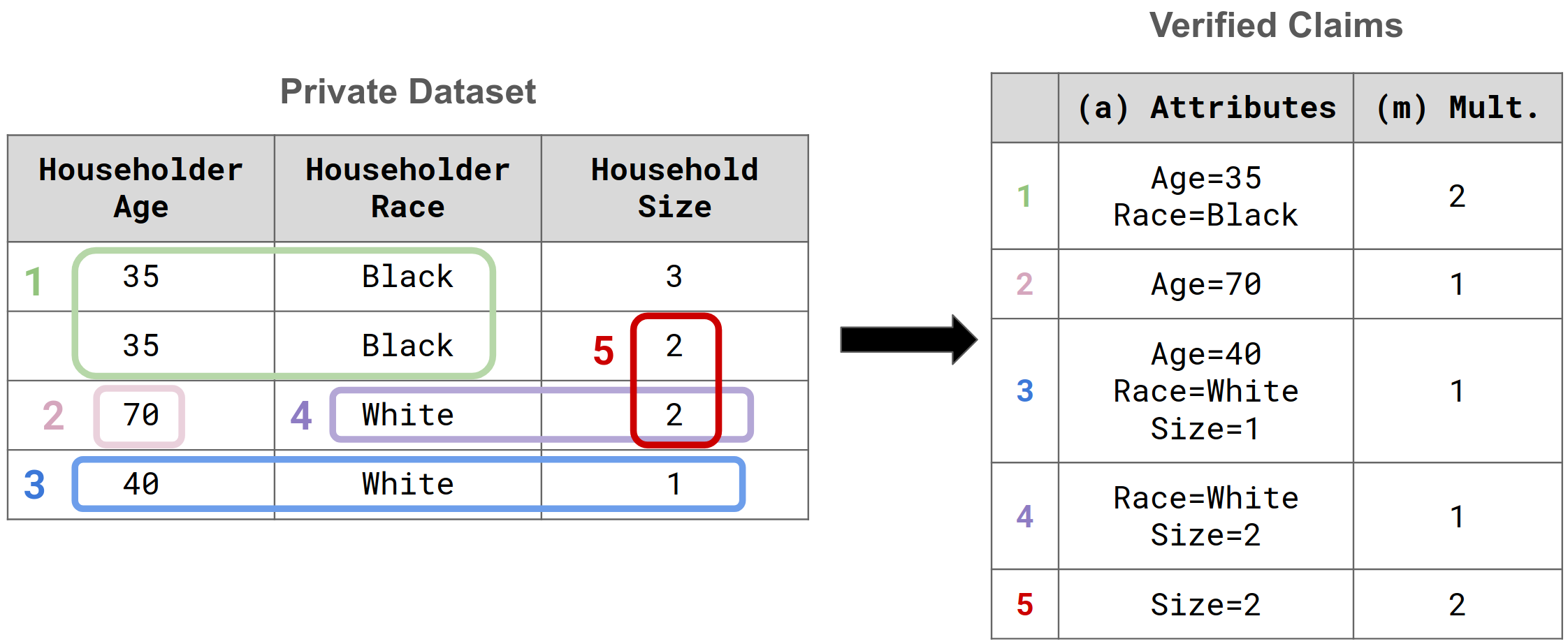
We introduce the problem of partial tabular data reconstruction to help better understand the vulnerability of data releases like the Decennial Census: rather than reconstructing the entire dataset with guaranteed correctness, the adversary aims to output verified claims about the data (see, e.g., Figure 1).
-
2.
We formulate an integer programming formulation that departs from the approaches of previous work [3, 10, 17] and allows us to tackle this problem. Specifically, given some set of aggregate statistics about the dataset, our method (1) generates a set of candidate claims and then (2) verifies whether these claims must be true according to the published statistics. In this paper, we consider claims about the number of rows with specific values in a subset of attributes, such as “in this block, there exists exactly one household whose head of the household is a 32-year old, Black woman.
-
3.
We evaluate our approach and that of previous work on the household-level data and tables from the Decennial Census release (2010 Summary File 1 (SF1)). We find that the method proposed in [2] for reconstructing entire blocks is ineffective in most cases—in our experiments, only one block (out of 50 total) could be reconstructed uniquely.
In contrast, our approach reconstructs many individual households with 100% certainty, demonstrating that partial reconstruction is still feasible (Table 1 provides examples of verified claims). Inspired by Cohen and Nissim [4], we focus on “singleton claims” (i.e., claims that single out exactly one individual in the dataset) and find that a nontrivial number of households can be reconstructed using some subset of columns that uniquely identifies them (i.e., singles them out).
| Block, Tract, | Reconstructed Information |
| County, State | |
| 1008, 010200, Baldwin, AL | A household with just a single female householder. She owns the home without a mortgage. The householder is white, of Hispanic or Latino origin, and is between 65 and 75 years old. |
| 3027, 271801, Baltimore City, MD | A renting household of size 2. It is a non-family household, and no one in the household is under 18 or over 65 years old. The householder is black, not of Hispanic or Latino origin, and between 25 and 34 years old. |
| 1006, 564502, Wayne, MI | A household of size 4 with a married couple that owns the home with a mortgage. No one in the household is over 65 years old, but there is at least one child under 18 years old. The householder is Black, not of Hispanic or Latino origin, and is between 45 and 54 years old. |
| 1049, 005828, Clark, NV | A married couple household (of unknown size) that does not own the home but also does not pay rent. No one in the household is over 65 years old, but there is at least one child under 18 years old. The householder of Hispanic or Latino origin and between 25 and 34 years old. Their race does not belong to one of the 5 major census race categories. |
| 1087, 940100, McKenzie, ND | A renting household of size 4. There is a cohabiting couple living with at least one child under 18 years old. No one in the household is over 65 years old. The householder is male, American Indian/Alaskan Native, not of Hispanic or Latino origin, and between 15 and 24 years old. |
Additional Related Work.
Real-world examples of privacy risks resulting from aggregate statistical releases have long been well-documented [18, 16, 2, 17, 11]. As a result, a long line of research, beginning with the seminal work of Dinur and Nissim [6], have both studied reconstruction attacks using public statistical information [8, 13, 14, 9] and developed notions for privacy guarantees—namely, Differential Privacy [7]. As mentioned previously, mitigating such privacy risks [17, 11, 5, 12, 3, 2] remains at the center of issues facing the U.S. Census Bureau, who has addressed such privacy concerns by incorporating Differential Privacy into the 2020 Decennial Census release [1]. Our work, in part, extends such findings, further demonstrating the risks that individuals face when aggregate statistics derived from them are released freely.
2 Preliminaries
In this setting, we have some dataset that is comprised of a multiset of records from a discrete domain . Let be some set of queries corresponding to the data domain , and let be a vector of aggregate statistics on dataset where each element is a statistic corresponding to a query in . Then, in its most general form, tabular data reconstruction can be set up as a simple constraint satisfaction problem (i.e., find any dataset that matches the statistics ),
| (1) |
In our work, we consider statistical queries , which we formally define as the following:
Definition 1 (Statistical Queries [15])
Given a predicate function , a statistical query (also known as a linear query or counting query) is defined for any dataset as
In other words, these queries are functions that count the number of records in that satisfy some given property (e.g., is female).
2.1 Record-level reconstruction.
In our work, we focus on record-level reconstruction, where the goal is to output claims about sets of rows . Suppose there exists columns in such that we rewrite . Let , where indicates that column can take on any value in . A vector in specifies a partial assignment to the attributes, and we say matches if they agree in all positions where .
Using this notation, we define to be the (reconstruction) claim that there exist exactly rows (e.g., in Figure1; claim 1) that match (e.g., describes a 35-year old, Black householder in Figure1; claim 1). We define to be the number of rows in that match . We say the claim is verified based on a summary if it holds for all data sets such that .
2.2 Guaranteeing the correctness of claims.
At a high level, to verify the correctness of any claim , one can ask the question: is it possible to construct a synthetic dataset that matches the published statistics, even when the multiplicity of number of rows with attributes does not equal ? If such a dataset does not exist, then must be correct. Concretely then, we check claims by again solving Problem 1 but with the added constraint that :
| (2) |
Note that in this setting, we can make use of all statistics (queries defined over all columns in ) available to us, even when verifying claims that are defined over only some subset of columns in .
3 Reconstruction via Integer Programming
In this section, we describe the implementation of our integer programming methods—namely, solving Problems 1 and 2.
At a high level, our approach can be broken down into two integer programming steps:
-
1.
Generate: We generate a list of claims that we then verify in step 2. Specifically, we solve Problem 1 times.111In Gurobi, we can simply set the solver to output up to solutions that satisfy the constraints. For each generated synthetic dataset , we identify all claims (i.e., all possible combinations of attributes and the corresponding multiplicities in ). We then take the intersection of the sets of claims to use as our final list.222The intersection contains all claims that are guaranteed to exist according to (explained further in 3.3).
-
2.
Verify: For each claim , we check if Problem 2 is feasible via integer programming. If no solutions can be found, then we conclude that must be correct.
3.1 Setup
One-hot encoded records.
Unlike prior work [3, 10, 17] which represents dataset as histograms over , our proposed integer programming optimization problem relies on one-hot encoded representations of . Specifically, let be the number of columns, which we denote as columns , in the domain. Given that all columns in are discrete, we represent records in as one-hot encoded vectors , where each encodes the column . Thus, we have rows where and . Finally, we let the matrix denote a one-hot encoded dataset with rows.
Query functions.
In this setting, we consider statistical queries (Definition 1) in the form of marginal queries where the predicate function is an indicator function for whether some set of columns takes on some set of values (note that is equivalent to what we call attributes in Section 2). For example, one can ask the marginal query about the columns Sex and Race: “How many people are (1) Female and (2) White or Black?" We note that one can break down any predicate into a set of sub-predicates, where each sub-predicate corresponds to one unique column pertaining to . Concretely, given some column and target values , we denote the sub-predicate function as
where is the value that takes on for column . Then, any predicate can be rewritten as the product of its sub-predicates (e.g. in the above example, can be written as the product of and ).
Given the one-hot encoded representation , can also be rewritten as a vector that takes on the value for indices in corresponding column and values (and otherwise). In this case, we can then rewrite the sub-predicate function as . Likewise, any predicate with sub-predicates can be rewritten as a matrix . Then can be written as where is a row vector of ones with length . Finally, a statistical query can be written as
| (3) |
In other words, we check whether each row in evaluates to .333We note that a simpler alternative to checking is to check whether the row product is equal to (i.e. ). However, our integer programming solver (Gurobi) does not support this operation.
Evaluating multiple queries.
In our setting, the set of queries contain queries that can differ in the number of sub-predicates (i.e., columns that are being asked about). For instance, using the above example data domain, one query may ask about the column Sex while another may ask about both Sex and Race. To handle such cases, given some set of queries , we let be the maximum number of sub-predicates for queries in . Then, in cases where some query predicate is comprised of sub-predicates, we can pad its matrix representation with rows corresponding to dummy sub-predicates . In this way, Equation 3 still holds (with being replaced by ).
Given that now the matrix representation for all queries in have the same shape, we can represent as a single -dimensional tensor . Then, we can calculate the statistics for all queries in by evaluating the product , where the -th query answer is
| (4) |
Note that we can interpret the vector as a boolean vector that checks whether record satisfies each of the sub-predicates for query . For ease of notation, we will assume going forward that refers to .
3.2 Generating Synthetic Data Using Aggregate Statistics (Problem 1)
We first describe how we set up the integer programming optimization problem for Problem 1—namely, how we represent the constraint . Using the notation in Section 3.1, we wish to find some synthetic dataset (whose one-hot representation we denote as ) such that .
As suggested above, we first evaluate whether each record satisfies all sub-predicates for each query (i.e., ). To do so, we want to add a helper binary variable such that
To enforce this relationship, we add the following constraints,
| (5) | ||||
| (6) |
so that evaluates query for record . Then, we add the constraints
| (7) |
to ensure that the aggregate count corresponding to query on the private dataset match that on .
Explanation. Suppose . Given that is binary, Equation 5 is true if and only if for all , thereby giving us . Moreover, Equation 6 is not violated since we have that
Similarly, if , then by Equation 6,
which, because is binary, can hold if and only if there exists some such that , meaning that . In this case, Equation 5 is not violated since (again, because can only take on the values and ).
3.2.1 Generating Unique Datasets
As stated previously, we set the integer programming solver to output up to solutions that we then use to generate claims to verify. However, in the one-hot encoded representation of datasets, two datasets with the same set of records that are ordered differently will be considered two unique solutions. To encourage unique solutions, we use a (fixed) vector of randomly generated integers as a hash function, where the hash value for any one-hot encoded record is . Then, for every , we add the constraint,
| (8) |
so that any solution outputted must have its records ordered by their hash values. While this approach is imperfect because, theoretically, different records in may map to the same hash value, we found it to be, in practice, a simple and computationally-efficient approach to filtering out duplicate solutions.
3.3 Generating Candidate Claims
Suppose our goal is to find all reconstruction sets that must exist in according to . Let us denote as the set of all for where (i.e., the set of all unique records and their multiplicities). Then the predicted multiplicity of any reconstruction set is exactly correct if . Using this notation, our goal is equivalent to finding all such that s.t. , . In other words, the only way we can be certain that some is contained in the private dataset is that it appears in all datasets where .
Therefore, to generate candidate records, one can simply generate a single synthetic dataset by solving Problem 1 and taking all unique records in and their multiplicities (i.e., ). Furthermore, to narrow down the set of candidates to check, one can generate many synthetic datasets and take their intersection since if there exists some such that , then violates the above condition.
Finally, we note that adjusting (number of synthetic datasets to output in the generate step allows one to trade-off computational resources between the two steps. Generating more synthetic datasets (i.e., decreasing the size of the intersection) will decrease the number of candidates that need to be verified.
3.4 Verifying the Correctness of Claims (Problem 2)
We now switch to setting up constraints for Problem 2—verifying whether some claim must be correct in the private dataset according to the released statistics . In this setting, we have a claim that is composed of attributes and claimed multiplicity of that record, . Suppose attributes are defined over some subset of columns indexed by the set (i.e, the columns ). Then we can define attributes as a vector , where is a one hot encoded representation of the attribute for column if all zeros otherwise.
In order to check whether is verifiable according to , we stipulate in the optimization problem that the number of times appears in cannot equal . If a feasible solution does not exist, then we can conclude that must be correct.
Constraints (part 1).
We first define a constant (used for ensuring other constraints are held) and let correspond to the list of indices that columns correspond to in . Next, let us introduce the binary variable , where
In other words, it indicates whether each column in matches the corresponding column value in . In addition, we introduce , which is a helper variable used to set properly in the constraints.
Now, we add constraints with and . Let be the number of (one-hot) indices we need to check. For each index , we add the constraints,
| (9) | ||||
| (10) | ||||
| (11) | ||||
| (12) |
Explanation. Consider the case when . Then from constraints 9 and 10, we have that and , which implies that . Thus, we know that the indicator for the feature value in the one-hot encoding of the candidate is equal to its corresponding value in row of . Constraints 11 and 12 give and . Given that is a large constant and that and are both in the domain , these constraints are also met.
Constraints (part 2).
Next, we add the binary variable , which is an indicator that checks whether each row matches on the attributes . If an entire row matches the attributes, then the entire corresponding row of should be equal to 1. This can be enforced with the following constraints:
| (13) | ||||
| (14) |
Constraints (part 3).
With indicating which rows match attributes , we now check whether the claimed multiplicity is correct by summing and checking if a there exists some dataset s.t. . If the solver is unable to find a solution under these constraints, then we conclude that dataset matching the statistics cannot exist without having exactly rows that match attributes .444 While it is not the focus of our work, we would like to point out that a similar integer programming problem can be set up to confirm that a candidate at multiplicity cannot exist by replacing constraints 15 and 16 so that they instead ensure . If the solver cannot find a solution where exactly rows match , then we conclude that candidate cannot exist at that multiplicity in the dataset.
Let be a scalar binary helper variable.
| (15) | |||
| (16) |
Explanation. If , we have and , which gives , enforcing .
Similarly, if , we have and , which also enforces .
4 Empirical Evaluation
Dataset.
In our experiments, we use the 2010 Privacy-Protected Microdata File, a synthetic dataset, statistically similar to the private 2010 Decennial Census microdata, that is generated and released by the U.S. Census Bureau. As the private 2010 Census microdata are not public, we treat the Privacy-Protected Microdata as the ground truth during evaluation. The PPMF (and Summary File 1, from which the PPMF is derived from) contains data for every housing unit in the United States. Each row of the PPMF represents one synthetic household response from the 2010 Decennial Census. There are 10 columns in total described by block-level tables (listed below), in contrast to the simpler, person-level data studied in prior work [3, 5] that only contains 4 columns. With the goal of reconstructing data at the block level, we select the block whose size is equal the median block size of the state containing it.
-
Tenure: One of 4 tenancy statuses: owned with mortgage, owned free and clear, rented, or occupied without payment of rent
-
Vacancy status: Not vacant, or one of 7 vacancy statuses: for rent, rented but not occupied, for sale, sold and not occupied, for seasonal or occasional use, for migrant workers, or other.
-
Household size: Size of household: 1, 2, 3, 4, 5, 6, or 7 or more
-
Household type: One of 7 types: married couple household, other family household (with a male/female householder), nonfamily household (with a male/female householder, living alone/not living alone).
-
Household type (including details about cohabitation and children): One of 12 types: married couple (with/without children 18), cohabiting couple (with/without children 18), no spouse/partner present (male/female householder, with own children 18/with relatives and without own children /only nonrelatives present/living alone)
-
Presence of people under 18 years in household: Whether or not one or more people younger than 18 are in the household
-
Presence of people over 65 years in household: Whether or not one or more people 65 years and over are in the household
-
Hispanic householder status: Whether or not the householder is of Hispanic origin,
-
Householder age: Age of the householder in one of 7 age buckets: 15-24, 24-35, …, 75-84, or 85 years and older.
-
Householder race: Race of the householder in one of 7 categories: White alone, Black alone, American Indian or Alaskan Native alone, Asian alone, Native Hawaiian or Pacific Islander alone, some other race alone, or two or more races.
Statistics.
In addition to the Privacy-Protected Microdata File, the U.S. Census Bureau releases aggregate statistics of features listed above, calculated from their private microdata, in the form of data tables. Each of these tables are released for every block and includes counts for the number of people corresponding to certain feature values defined by the table. For example, cell 2 of table H14 contains the count of owner-occupied family households containing a married couple and whose householder is between the ages of 35 and 64. Utilizing all tables tabulated at the block-level, we have statistics / queries as inputs to our integer programming approach. We list the tables names below, along with the descriptors given by the Census Bureau.
-
P16: Household type,
-
P16 A-G: Household type (iterated by race),
-
P16 H: Household type for households with a householder who is Hispanic or Latino,
-
P16 I-O: Household type for households with a householder who is not Hispanic or Latino (iterated by race),
-
P16 P-V: Household type for households with a householder who is Hispanic or Latino (iterated by race),
-
P19: Households by presence of people 65 years and over, household size, and household type,
-
P20: Households by type and presence of own children under 18 years,
-
P21: Households by presence of people under 18 years,
-
H1: Housing units (total count),
-
H3: Occupancy status,
-
H4: Tenure,
-
H4 A-G: Tenure (iterated by race),
-
H4 H: Tenure of housing units with a householder who is Hispanic or Latino,
-
H4 I-O: Tenure of housing units with a householder who is not Hispanic or Latino (iterated by race),
-
H4 P-V: Tenure of housing units with a householder who is Hispanic or Latino (iterated by race),
-
H5: Vacancy status of vacant housing units,
-
H6: Race of householder,
-
H7: Hispanic or Latino origin of householder by race of householder,
-
H9: Household size,
-
H10: Tenure by race of householder,
-
H11: Tenure by Hispanic or Latino origin of Householder,
-
H12: Tenure by household size,
-
H12 A-G: Tenure by household size (iterated by race),
-
H12 H: Tenure by household size of households with a householder who is Hispanic or Latino,
-
H12 I: Tenure by household size of households with a householder who is White only and not Hispanic or Latino,
-
H13: Tenure by age of householder,
-
H13 A-G: Tenure by age of householder (iterated by race),
-
H13 H: Tenure by age of householder for housing units with a householder who is Hispanic or Latino,
-
H13 I: Tenure by age of householder for housing units with a householder who is White alone and not Hispanic or Latino,
-
H14: Tenure by household type by age of householder,
-
H15: Tenure by presence of people under 18 years, excluding householders, spouses, and unmarried partners,
IP Solver.
We use Gurobi Optimizer to solve our integer programming optimization problems. We specify parameters “feasibility tolerance” and “integer feasibility tolerance” to their smallest value of to enforce constraints as tightly as possible, and “pool search mode” to 2 to find as many best solutions as defined by “pool solutions”, which is set to when generating candidates and to 1 when validating candidates. We also set the time limit parameter as some computations may take too long, particularly for larger blocks.
4.1 Baselines
While we contend that finding any records that can be reconstructed confidence is already interesting, we would like to further provide context for our results by providing some baseline measure for how likely a block contains any reconstructed record. To do so, we calculate the probability of each verified claim being correct in a block of size that is randomly sampled from the tract and state that the households resides in.
Let us assume that records in a block are drawn from some prior distribution . Then the multiplicity of some candidate record appearing in a block of size follows the binomial distribution,
| (17) |
where is the probability of a single record being drawn from the prior .
In typical settings in which an adversary has no prior information about the block of interest, is simply the uniform distribution (i.e., , where is the one-hot encoded representation of with columns ). However, this comparison is uninteresting since is close to in such cases. In our evaluation, we instead construct a setting in which the prior distribution of the tract and state (similar to Dick et al. [5]) that some block belongs to is known. Let and be the set of records in the tract and state. Then, we can express as
for and , respectively, and use Equation 17 to calculate the baseline probability for any given candidate claim .
5 Results
We now present our empirical results for verified singleton claims. We note that there exists claims can be “read” directly off the statistics.555e.g., a table reporting 2 White householders already tells us that the claim must be correct.Thus, given that generating and verifying such claims is trivial, we remove them from all plots and tables reported in our evaluation.
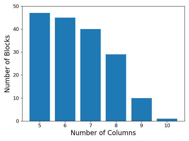
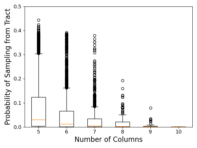
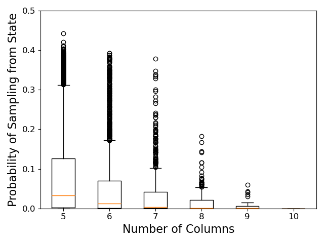
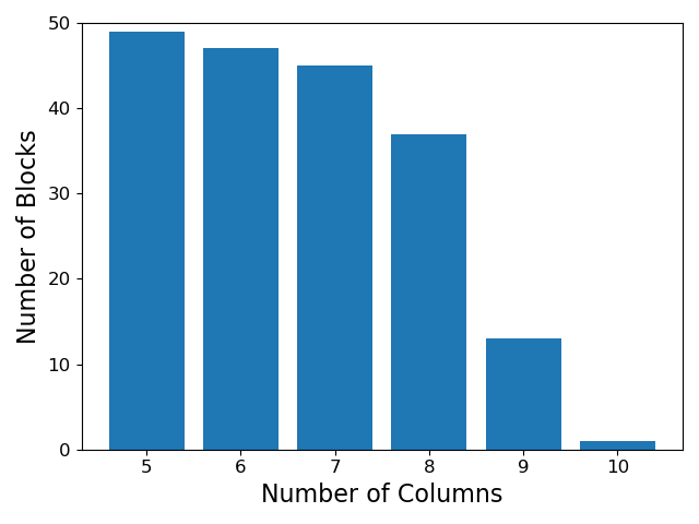
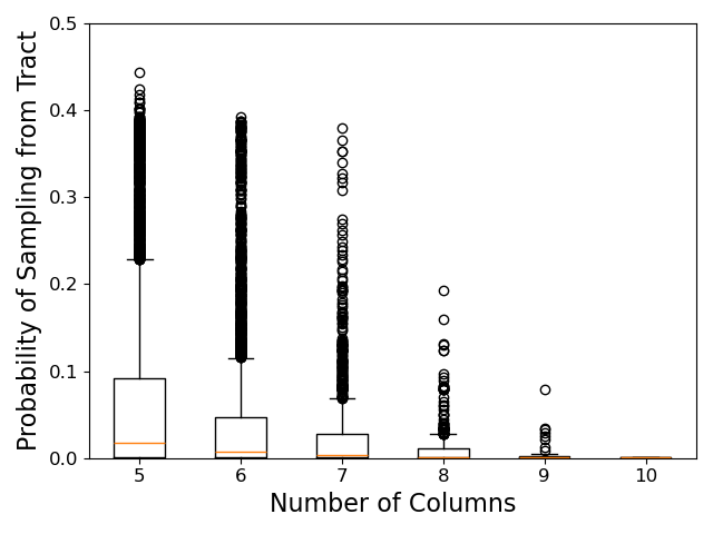
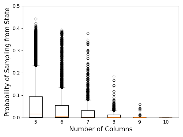
In Figure 2(a), we report the number of blocks (y-axis) for which we can reconstruct some set of columns (x-axis) for at least one household. We find that while reconstruction (with 100% certainty) of all 10 columns is often not possible, we can reconstruct and verify at least one singleton claim with up to 8 columns in the majority of the blocks. For claims describing 5 columns, we can reconstruct at least one households in over 90% of the blocks. In Figures 2(b) and 2(c), we evaluate the baseline probabilities for all claims verified by our approach to understand how ”surprising“ they are, given some prior information about the state and tract demographics. We find that in general, these baselines probabilities are quite low, with the median being under 5% for all number of columns (and nearly 0% for 7 or more columns). Even among outliers, the chances of randomly sampling a block where such claims are true never exceeds 50%.
Finally, in Table 2 we report the number of unique households that we reconstruct, given some number of columns. Here, instead of counting the total number of claims we verify, we total up how many households are covered by the claims. 666In Figure 1, the total multiplicity of claims 2 and 4 is 2. However, only 1 households is represented among these claims (row 3 on the left-hand table). Thus, Table 2 groups the verified claims by the number of columns (in ) and reports the number of households (in the left-hand table) that are represented in the claims. Again, despite the difficulty of reconstructing all 10 columns of households, we find that a non-trivial (over 10%) of households are uniquely identifiable by some claim that describes 8 columns. This proportion increases to a third when looking at claims that describe 5 columns.
| # of households identified by | |||||||
| # of households | verified claims w/ columns | ||||||
| =5 | 6 | 7 | 8 | 9 | 10 | ||
| Total | 486 | 166 | 148 | 109 | 61 | 19 | 2 |
| Avg. per block | 9.72 | 3.32 | 2.96 | 2.18 | 1.22 | 0.38 | 0.04 |
6 Conclusion
In conclusion, our work introduces the problem of partial tabular data reconstruction and proposes an integer programming approach that reconstructs individual records with guaranteed correctness. Evaluating on the housing-level microdata and tables from the U.S. Decennial Census, we demonstrate that one can still (partially) reconstruct individual households with certainty, even when many different blocks may satisfy the published statistics. We note that one limitation of using integer programming in our approach is that evaluating on larger datasets (more rows or columns) or sets of statistics may induce computational costs far more demanding than those required for our experiments. Nevertheless, our experiments show that for releases like the decennial census, in which the average dataset (i.e., block) is relatively small, reconstruction is very much possible while being computationally inexpensive. Overall, we contend that our initial work on partial reconstruction represents just the tip of the iceberg in terms of communicating the privacy risks that come with releasing aggregate information. We hope that our work inspires future research to build upon such notions of partial reconstruction (e.g., extending our approach to other data domains or using our approach of singling out households as part of larger, more systematic study on the dangers of linkage attacks).
References
- Abowd [2018] John M. Abowd. The U.S. census bureau adopts differential privacy. In ACM International Conference on Knowledge Discovery & Data Mining, page 2867, 2018.
- Abowd and Hawes [2023] John M Abowd and Michael B Hawes. Confidentiality protection in the 2020 us census of population and housing. Annual Review of Statistics and Its Application, 10(1):119–144, 2023.
- Abowd et al. [2023] John M Abowd, Tamara Adams, Robert Ashmead, David Darais, Sourya Dey, Simson L Garfinkel, Nathan Goldschlag, Daniel Kifer, Philip Leclerc, Ethan Lew, et al. The 2010 census confidentiality protections failed, here’s how and why. Technical report, National Bureau of Economic Research, 2023.
- Cohen and Nissim [2020] Aloni Cohen and Kobbi Nissim. Towards formalizing the gdpr’s notion of singling out. Proceedings of the National Academy of Sciences, 117(15):8344–8352, 2020.
- Dick et al. [2023] Travis Dick, Cynthia Dwork, Michael Kearns, Terrance Liu, Aaron Roth, Giuseppe Vietri, and Zhiwei Steven Wu. Confidence-ranked reconstruction of census microdata from published statistics. Proceedings of the National Academy of Sciences, 120(8):e2218605120, 2023.
- Dinur and Nissim [2003] Irit Dinur and Kobbi Nissim. Revealing information while preserving privacy. In Proceedings of the twenty-second ACM SIGMOD-SIGACT-SIGART symposium on Principles of database systems, pages 202–210, 2003.
- Dwork et al. [2006] Cynthia Dwork, Frank McSherry, Kobbi Nissim, and Adam Smith. Calibrating noise to sensitivity in private data analysis. In Theory of Cryptography: Third Theory of Cryptography Conference, TCC 2006, New York, NY, USA, March 4-7, 2006. Proceedings 3, pages 265–284. Springer, 2006.
- Dwork et al. [2007] Cynthia Dwork, Frank McSherry, and Kunal Talwar. The price of privacy and the limits of lp decoding. In Proceedings of the thirty-ninth annual ACM symposium on Theory of computing, pages 85–94, 2007.
- Dwork et al. [2017] Cynthia Dwork, Adam Smith, Thomas Steinke, and Jonathan Ullman. Exposed! a survey of attacks on private data. Annual Review of Statistics and Its Application, 4(1):61–84, 2017.
- Dwork et al. [2024] Cynthia Dwork, Kristjan Greenewald, and Manish Raghavan. Synthetic census data generation via multidimensional multiset sum. arXiv preprint arXiv:2404.10095, 2024.
- Flaxman and Keyes [2025] Abraham Flaxman and Os Keyes. The risk of linked census data to transgender youth: A simulation study. Journal of Privacy and Confidentiality, 15(1), 2025.
- Garfinkel et al. [2019] Simson Garfinkel, John M Abowd, and Christian Martindale. Understanding database reconstruction attacks on public data. Communications of the ACM, 62(3):46–53, 2019.
- Kasiviswanathan et al. [2010] Shiva Prasad Kasiviswanathan, Mark Rudelson, Adam Smith, and Jonathan Ullman. The price of privately releasing contingency tables and the spectra of random matrices with correlated rows. In Proceedings of the forty-second ACM symposium on Theory of computing, pages 775–784, 2010.
- Kasiviswanathan et al. [2013] Shiva Prasad Kasiviswanathan, Mark Rudelson, and Adam Smith. The power of linear reconstruction attacks. In Proceedings of the twenty-fourth annual ACM-SIAM symposium on Discrete algorithms, pages 1415–1433. SIAM, 2013.
- Kearns [1998] Michael Kearns. Efficient noise-tolerant learning from statistical queries. Journal of the ACM (JACM), 45(6):983–1006, 1998.
- Narayanan and Shmatikov [2008] Arvind Narayanan and Vitaly Shmatikov. Robust de-anonymization of large sparse datasets. In 2008 IEEE Symposium on Security and Privacy (sp 2008), pages 111–125. IEEE, 2008.
- Steed et al. [2024] Ryan Steed, Diana Qing, and Zhiwei Steven Wu. Quantifying privacy risks of public statistics to residents of subsidized housing. arXiv preprint arXiv:2407.04776, 2024.
- Sweeney [1997] Latanya Sweeney. Weaving technology and policy together to maintain confidentiality. The Journal of Law, Medicine & Ethics, 25(2-3):98–110, 1997.
Appendix A Additional Results
In the main body of our work, we focus on “singling out” (singleton claims). However, we note that data reconstruction for multiplicity can be equally interesting (or privacy violating).
Thus, we present in Figure 3 and Table 3 results for all claims (not just singletons). In general, we make conclusions similar to those in Section 4. The baseline probabilities of most claims are still extremely small, and as expected, more claims (about more households) can be made. For example, Table 3 shows that now, almost 90% households are represented among claims describing columns.
| # of households identified by | |||||||
| # of households | verified claims w/ columns | ||||||
| =5 | 6 | 7 | 8 | 9 | 10 | ||
| Total | 486 | 431 | 379 | 274 | 179 | 30 | 2 |
| Avg. per block | 9.72 | 8.62 | 7.58 | 5.48 | 3.58 | 0.60 | 0.04 |