Graph Synthetic Out-of-Distribution Exposure with Large Language Models

Abstract

Out-of-distribution (OOD) detection in graphs is critical for ensuring model robustness in open-world and safety-sensitive applications. Existing approaches to graph OOD detection typically involve training an in-distribution (ID) classifier using only ID data, followed by the application of post-hoc OOD scoring techniques. Although OOD exposure—introducing auxiliary OOD samples during training—has proven to be an effective strategy for enhancing detection performance, current methods in the graph domain generally assume access to a set of real OOD nodes. This assumption, however, is often impractical due to the difficulty and cost of acquiring representative OOD samples. In this paper, we introduce GOE-LLM, a novel framework that leverages Large Language Models (LLMs) for OOD exposure in graph OOD detection without requiring real OOD nodes. GOE-LLM introduces two pipelines: (1) identifying pseudo-OOD nodes from the initially unlabeled graph using zero-shot LLM annotations, and (2) generating semantically informative synthetic OOD nodes via LLM-prompted text generation. These pseudo-OOD nodes are then used to regularize the training of the ID classifier for improved OOD awareness. We evaluate our approach across multiple benchmark datasets, showing that GOE-LLM significantly outperforms state-of-the-art graph OOD detection methods that do not use OOD exposure and achieves comparable performance to those relying on real OOD data.

1 Introduction

Graph is a powerful and expressive data structure for modeling relationships among entities, with widespread applications in social networks, citation networks, recommendation systems, biological networks, and more [21, 31, 23, 22]. In many real-world scenarios, nodes in graphs are accompanied by rich textual attributes—such as user bios, paper abstracts, or product descriptions—giving rise to text-attributed graphs (TAGs) [28, 26]. These graphs contain both structural and semantic information, enabling more nuanced learning and inference tasks.

Recently, the task of Out-of-Distribution (OOD) detection in graphs [20, 10, 25, 30, 24] has gained significant attention due to its importance in safety-critical and open-world settings. In graph-based OOD detection, the goal is to identify nodes whose distribution significantly deviates from the in-distribution (ID) training classes. This task is particularly relevant in real-world applications where unseen or anomalous entities may appear during inference—such as emerging users in social platforms, new research domains in citation graphs, or novel products in e-commerce graphs. Detecting such OOD nodes is critical for ensuring model robustness, maintaining prediction confidence, and preventing harmful or unreliable decisions.

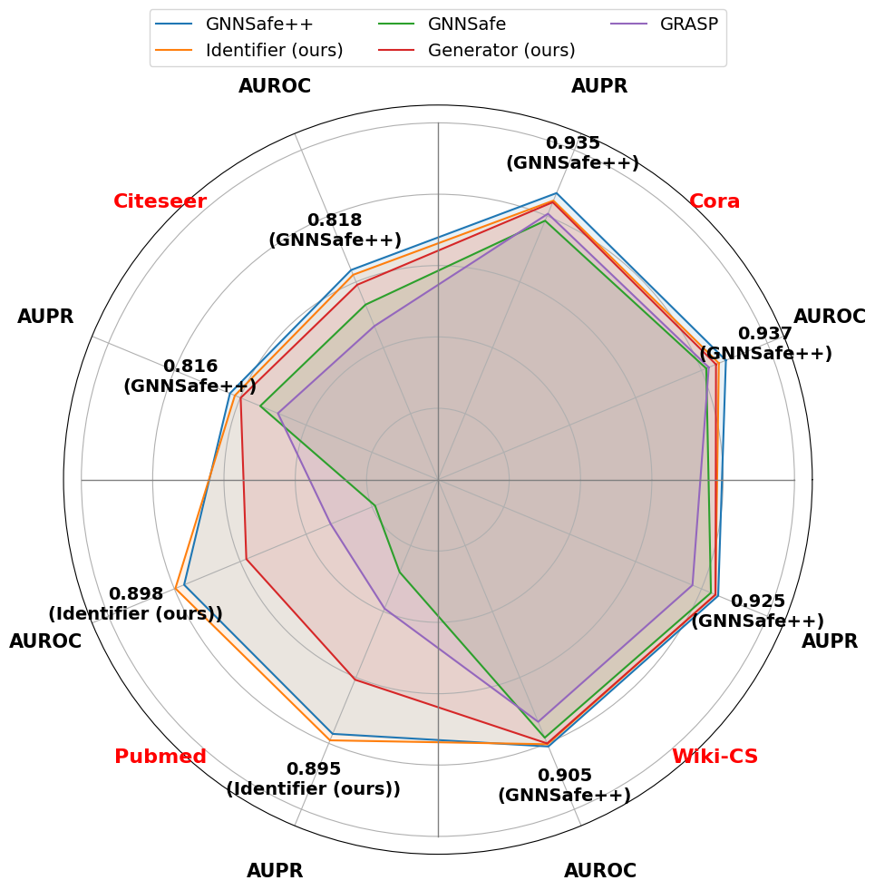
Figure 1: Our graph OOD detection method does not rely on any real OOD nodes for training, yet achieves significantly better OOD detection performance than baseline methods and performs comparably to the approach that use real OOD nodes (GNNSafe++) for exposure.

Current graph OOD detection approaches commonly adopt a semi-supervised, transductive setting, in which all nodes are available during training, but only a subset of class labels corresponding to ID classes is provided. However, relying solely on ID data during training limits a model’s ability to generalize to unseen inputs with distribution shifts, often resulting in overconfident predictions on OOD nodes [8]. Consequently, post-hoc OOD scoring methods applied to such models may perform suboptimally, especially when OOD instances share structural or semantic similarities with ID data. A prominent approach to improving OOD detection is OOD exposure, where auxiliary OOD samples are introduced during training to help the model learn to distinguish between ID and OOD inputs. Image-based OOD detection methods [7, 29] have explored leveraging external OOD datasets and augmenting ID samples through mixing strategies. In addition, [3] incorporates unlabeled wild data to enhance classifier robustness. However, these approaches are fundamentally limited by the availability and representativeness of suitable OOD data.

While effective, traditional OOD exposure methods typically rely on the availability of real, labeled OOD data—an assumption that is often unrealistic or costly to satisfy, especially in graph settings [20] where OOD nodes may not be well-defined or easily sourced. Some recent works in the image and text domains have explored pseudo-OOD generation [17, 1, 2, 4, 19], where synthetic OOD samples are created to simulate distributional shifts, reducing reliance on real OOD data. For example, [1] leverage Large Language Models (LLMs) to create high-quality OOD proxies for text OOD detection. [18] propose a novel algorithm for generating effective OOD samples for training an $n+1$-class classifier for OOD detection. EOE [2] harness the expert knowledge embedded in LLMs to envision outlier exposure on image data without relying on actual or auxiliary OOD data. However, none of these methods are tailored for graph data. Unlike images or text where instances are independent, graph data exhibits complex relational dependencies — each node is inherently influenced by its neighboring nodes. This unique characteristic poses additional challenges for OOD exposure on graphs, making it non-trivial to directly adapt existing methods that overlook graph structural information.

In this paper, we explore the task of OOD detection on TAGs and propose using LLMs for zero-shot OOD annotation and pseudo-OOD node generation. Given their strong zero-shot capabilities, we aim to leverage LLMs to generate OOD supervision signals and enrich the training dataset. Specifically, we design two pipelines for OOD exposure without relying on real OOD nodes. The first method utilizes an LLM to identify potential OOD nodes in the graph. Specifically, we begin by randomly selecting a small subset of unlabeled nodes. Then, we prompt the LLM to perform zero-shot OOD detection. For each selected node, we let LLM say “none” if it predicts that the node does not belong to any of the ID classes. The noisy OOD nodes identified by the LLM are subsequently treated as real OOD nodes for OOD exposure. The second method leverages the LLM to generate text descriptions of pseudo-OOD nodes based on its inherent knowledge of the relevant domains. These pseudo-OOD nodes are then inserted into the original graph using graph structure learning methods. Finally, the augmented graph, containing both ID and OOD labels, is used to train the ID classifier. As shown in Fig. 1, our proposed graph OOD detection method operates without access to any real OOD nodes during training, yet it significantly outperforms baseline methods without OOD exposure and achieves performance comparable to approaches that rely on real OOD data. Our framework offers a practical and scalable solution for effective OOD detection in real-world, open-world graph applications enriched with textual information. We summarize our key contributions as follows:

• To the best of our knowledge, we are the first to leverage LLMs for OOD exposure in graph OOD detection. By utilizing the zero-shot learning capabilities of LLMs, our method eliminates the need for any real OOD nodes during training.

• We propose two approaches for graph OOD exposure without relying on real OOD nodes: using an LLM as a pseudo-OOD node identifier and as a pseudo-OOD node generator.

• Experimental results demonstrate that our method significantly outperforms baselines without OOD exposure and achieves comparable performance to methods that use real OOD nodes for exposure.

2 Related Works

2.1 Graph OOD Detection

Detecting OOD samples, for which models should exhibit low confidence, has been widely explored in recent literature. GNNSafe [20] reveals that standard GNN classifiers possess inherent OOD detection capabilities and introduces an energy-based discriminator trained with standard classification loss. OODGAT [16] explicitly separates inliers from outliers during feature propagation and addresses node classification and outlier detection within a unified framework. GRASP [10] examines the benefits of OOD score propagation and establishes theoretical conditions for its effectiveness. Additionally, it proposes an edge augmentation strategy with theoretical guarantees for post-hoc node-level OOD detection. GNNSafe++ [20] use real OOD nodes as training data to incorporate an auxiliary regularization term when training data contains OOD observation as outlier exposure. In this paper, we design effective OOD exposure methods without relying on real OOD samples.

2.2 OOD Detection Methods with OOD Exposure

A line of OOD detection methods leverages a set of real OOD samples during training to help models learn the distinction between ID and OOD data [27]. OECC [13] observes that incorporating an additional regularization term for confidence calibration can further enhance the performance of outlier exposure. MixOE [29] extend the coverage of the OOD space by mixing ID data with training-time outliers. These mixed samples are used to regularize the model’s behavior, encouraging a smooth decay in prediction confidence as inputs shift from ID to OOD.

However, previous OOD exposure methods make a strong assumption about the availability of OOD training data, which is often infeasible in practice. Another line of research focuses on pseudo-OOD generation, where synthetic OOD samples are created to simulate real-world scenarios and enable ID/OOD separability. Approaches like VOS [4] generate OOD representations without relying on external datasets, making them highly practical when real OOD data is unavailable. More recently, LLMs have been used to generate pseudo-OOD data for text tasks [1], further reducing dependence on manually curated OOD samples. However, existing graph OOD detection methods with OOD exposure typically assume access to a real OOD node set that is accurately labeled by humans. In this paper, we propose using LLMs for both zero-shot OOD detection and pseudo-OOD node generation, thereby eliminating the need for any real OOD nodes during OOD exposure.

3 Methodology

3.1 Preliminary

Our study focus on OOD detection on TAGs. A TAG is represented as $G_{T}=(\mathcal{V},\mathbf{A},\mathbf{T},\mathbf{X})$. The set of nodes is $\mathcal{V}=\{v_{1},\dots,v_{n}\}$, where each node is associated with raw text attributes $\mathbf{T}=\{t_{1},t_{2},\dots,t_{n}\}$. These text attributes can be converted into sentence embeddings $\mathbf{X}=\{x_{1},x_{2},\dots,x_{n}\}$ using SentenceBERT [14]. The adjacency matrix $\mathbf{A}\in\{0,1\}^{n\times n}$ encodes graph connectivity, where $\mathbf{A}[i,j]=1$ indicates an edge between nodes $v_{i}$ and $v_{j}$.

Node-level Graph OOD Detection. We have a limited labeled node set $\mathcal{V}_{I}$ and a large unlabeled node set $\mathcal{V}_{U}$. Each labeled node belongs to one of $K$ known classes $Y_{I}=\{y_{k}\}_{k=1}^{K}$, while an unlabeled node may belong to an unknown class not included in $Y_{I}$. The problem is framed in a semi-supervised, transductive setting, where we can access the full set of nodes during training but only a subset of class labels (ID classes). Our goal is, for each node $v_{i}\in\mathcal{V}_{U}$, determine whether it is from the ID $K$ known classes or from the OOD classes.

3.2 Graph OOD Detection with Pseudo-OOD Exposure

OOD exposure helps the model learn a tighter and more precise boundary around ID data in the feature space. For node-level OOD detection, we first employ a two-layer GCN as the ID classifier and train it on the labeled ID node set $\mathcal{V}_{I}$ using the following supervised classification loss:

$$\mathcal{L}_{\text{sup}}=-\frac{1}{|\mathcal{V}_{I}|}\sum_{i\in\mathcal{V}_{I}}\sum_{k=1}^{K}y_{ik}\log\hat{y}_{ik}$$ (1)

After the ID classifier is well-trained, any post-hoc OOD detection method can be applied to compute OOD scores for all nodes. For example, when using the negative energy score [9] as the OOD score, assume that the classifier outputs logits $z_{i}\in\mathbb{R}^{K}$ for node $v_{i}$ over $K$ ID classes. The OOD score of $v_{i}$ is then computed as:

$$S_{\text{OOD}}(v_{i})=-E(v_{i})=\log\sum_{k=1}^{K}\exp(z_{ik})$$ (2)

To perform OOD exposure, we introduce a regularization loss $\mathcal{L}_{\text{expo}}$ to impose hard constraints on the OOD score. This loss bounds the OOD scores for ID data, i.e., labeled instances in $\mathcal{V}_{I}$, and OOD data, represented by auxiliary training instances $\mathcal{V}_{O}$ from a distinct distribution. The final training objective is formulated as $\mathcal{L}_{\text{sup}}+\lambda\mathcal{L}_{\text{expo}}$, where $\lambda$ is a trade-off weight. We instantiate the regularization loss using bounding constraints on the OOD scores:

$$\mathcal{L}_{\text{expo}}=\frac{1}{|\mathcal{V}_{I}|}\sum_{v_{i}\in\mathcal{V}_{I}}\left(\operatorname{ReLU}\left(S_{\text{OOD}}(v_{i})-s_{\text{id}}\right)\right)^{2}+\frac{1}{|\mathcal{V}_{O}|}\sum_{v_{j}\in\mathcal{V}_{O}}\left(\operatorname{ReLU}\left(s_{\text{ood}}-S_{\text{OOD}}(v_{j})\right)\right)^{2}$$ (3)

where $s_{\text{id}}$ and $s_{\text{ood}}$ are two margin parameters. The set $\mathcal{V}_{O}$ may consist of either real OOD nodes annotated by humans or synthetic OOD nodes generated by models such as LLMs.

Figure 2: An overview of our framework GOE-LLM. We design two methods for graph OOD exposure without using real OOD nodes: LLM as OOD nodes’ identifier and LLM as OOD nodes’ generator. The first method employs an LLM to identify potential OOD nodes from the initially fully unlabeled graph. These nodes are then used as pseudo-OOD samples to regularize the training of the ID classifier. The second method prompts the LLM to generate textual descriptions of synthetic OOD nodes, which are subsequently embedded and inserted into the original graph to enrich OOD information during ID classifier training.

3.3 Identify OOD Nodes with LLMs

In this setting, instead of exposing real OOD nodes to the ID classifier, we assume that we have no access to real OOD nodes, including the names of OOD classes. Given the transductive nature of the graph learning setting, we propose to instruct LLMs to identify potential OOD nodes in the original graph and leverage these identified nodes to regularize the training of the ID classifier. Specifically, we first randomly sample a small set of nodes $\mathcal{V}_{U}^{\text{sampled}}$ from $\mathcal{V}_{U}$ and have the LLM annotate them. The LLM is only provided with ID knowledge (ID class names) and prompted to determine whether the unlabeled query node belongs to an ID class, using its textual information. We instruct the LLM to output "none" if it determines that the node does not belong to any predefined ID class. After that, we select the nodes identified by the LLM as OOD to form the pseudo-OOD node set $\mathcal{V}_{O}$, as shown in Eqn. 4. Using this annotated set $\mathcal{V}_{O}$, we then train the ID classifier with Eqn. 3.

$$\mathcal{V}_{O}=\{v\in\mathcal{V}_{U}^{\text{sampled}}\mid\text{LLM}(\text{prompt}(v,\mathcal{C}_{\text{id}}))=\text{"none"}\}$$ (4)

where $\mathcal{C}_{\text{id}}$ denotes the set of ID category names.

3.4 Generate OOD Nodes with LLMs

Instead of using LLMs to identify potential OOD nodes in the graph, we propose an alternative approach that leverages LLMs to generate pseudo-OOD nodes and insert them into the original graph for OOD exposure. These generated pseudo-OOD nodes constitute the OOD instances $\mathcal{V}_{O}$ in Eqn. 3. In this setting, we assume access only to the label names of the classes, without any real OOD nodes. We generate $M$ samples with an LLM for each OOD class, leveraging the LLM’s inherent large-scale knowledge of the respective class domains. The generated text descriptions of the pseudo-OOD nodes are denoted by $\mathbf{T}^{\text{ood}}$, and this process is formalized in Eqn. 5.

$$\mathcal{V}_{O}=\{v_{m}^{\text{ood}}\mid\mathbf{T}_{m}^{\text{ood}}=\text{LLM}(\text{prompt}(c)),\ 1\leq m\leq M,\ c\in\mathcal{C}_{\text{ood}}\}$$ (5)

where $\mathcal{C}_{\text{ood}}$ denotes the set of OOD category names. By applying SentenceBERT [14] to $\mathbf{T}^{\text{ood}}$, we obtain the embeddings of the pseudo-OOD nodes as $\mathbf{X}^{\text{ood}}$. The complete set of node embeddings is then given by $\mathbf{X}_{\text{aug}}=\mathbf{X}\mathbin{\|}\mathbf{X}^{\text{ood}}$. Optionally, with graph structure learning, we can incorporate the pseudo-OOD nodes into the original graph to better propagate information through the new graph structure, denoted as $\mathbf{A}_{\text{aug}}$. One way to construct $\mathbf{A}_{\text{aug}}$ is by creating edges based on the similarity of node embeddings. Alternatively, a negative sampling-based link prediction task can be performed to infer potential links. Using $\mathbf{X}_{\text{aug}}$ and $\mathbf{A}_{\text{aug}}$, we then train the ID classifier on the augmented graph.

3.5 Synthetic OOD Model

Thus far, we have proposed using pseudo-OOD nodes to regularize the training of a $K$-class ID classifier and applying post-hoc OOD detectors on top of the well-trained ID classifier for OOD detection. The main advantage of this approach is that it does not require modifying the network architecture of the ID classifier. However, it introduces a trade-off weight $\lambda$ in the loss function. Intuitively, if $\lambda$ is too large, it may degrade ID classification performance. Conversely, if $\lambda$ is too small, the OOD information may not be sufficiently exposed to the ID classifier to improve its OOD awareness. To address this, we provide two alternative approaches that leverage both labeled ID nodes and synthetic noisy OOD nodes to train a model with enhanced OOD awareness.

The first approach involves adding a binary classification layer on top of the standard ID classifier trained using Eqn. 1 to predict OOD scores. Specifically, we first train the ID classifier using labeled ID nodes. Once trained, we freeze the ID classifier and fit the weights of the binary OOD detector using a small set of labeled ID nodes along with the pseudo-OOD samples. The key advantage of this method is that it preserves the ID predictions of the pre-trained classifier while equipping the model with the capability to detect OOD nodes through the additional binary layer. The second approach extends the ID classifier into a $(K+1)$-way classification model, where the first $K$ classes correspond to the ID classes and the $(K+1)$-th class represents the OOD class. The model is trained using both labeled ID nodes and pseudo-OOD nodes under a unified cross-entropy loss. The primary advantage of this joint classification approach lies in its flexibility to simultaneously learn accurate ID predictions while distinguishing between ID and OOD nodes, thereby enhancing overall performance.

4 Experiments

4.1 Experimental Setup

Datasets We utilize the following TAG datasets, which are commonly used for node classification: Cora [11], Citeseer [5], Pubmed [15] and Wiki-CS [12]. The dataset descriptions are in Appendix B. We follow prior work [16] by splitting the node classes into ID and OOD classes, ensuring that the number of ID classes is at least two to support the ID classification task. The specific class splits and ID ratios are detailed in Appendix A.

Training and Evaluation Splits For each dataset with $K$ ID classes, we use $20\times K$ of ID nodes for training. Additionally, we randomly select $10\times K$ of ID nodes along with an equal number of OOD nodes for validation. The test set consists of 500 randomly selected ID nodes and 500 OOD nodes. All experiments are repeated with five random seeds, and results are averaged.

Baselines We compare GOE-LLM with the following baselines: (1) MSP [6], (2) Entropy, (3) Energy [9], (4) GNNSafe [20], and (5) GRASP [10], all of which are post-hoc OOD detection methods without exposure. Additionally, we include GNNSafe++ [20], a state-of-the-art method that leverages real OOD samples for exposure.

LLM-Powered OOD Exposure We use GPT-4o-mini for both pseudo-OOD identification and generation. For node identification, we randomly sample 200 unlabeled nodes per dataset and prompt the LLM to label them as ID or OOD. Nodes predicted as OOD are used as pseudo-OOD exposure data. For pseudo-OOD generation, we prompt the LLM to generate $10\times K_{\text{ood}}$ nodes, where $K_{\text{ood}}$ is the number of OOD classes. Text is embedded using SentenceBERT [14], and optionally inserted into the graph using similarity-based edge construction.

Implementation details All ID classifiers are implemented using 2-layer GCNs with hidden dimension 32. We use Adam optimizer with learning rate 0.01, dropout rate 0.5, and weight decay of 5e-4. For all OOD exposure methods, the trade-off weight $\lambda$ in the loss function is selected from $\{0.01,0.05\}$ based on the results of the validation set. All experiments are conducted on hardware equipped with an NVIDIA RTX 4080 Ti.

Evaluation Metrics For the ID classification task, we use classification accuracy (ID ACC) as the evaluation metric. For the OOD detection task, we employ three commonly used metrics from the OOD detection literature [20]: the area under the ROC curve (AUROC), the precision-recall curve (AUPR), and the false positive rate when the true positive rate reaches 95% (FPR@95). In all experiments, OOD nodes are considered positive cases.

4.2 Main Results

Table 1 presents the performance of various OOD detection methods across four datasets. From the results, we make several key observations:

Effectiveness of LLM-driven OOD Exposure. Both variants of GOE-LLM —GOE-LLM-Identifier and GOE-LLM-Generator—consistently outperform all baseline methods that do not utilize OOD exposure. For example, on the Pubmed dataset, GOE-LLM-Identifier achieves an AUROC of 0.8985, significantly surpassing GRASP (0.6627), the best-performing baseline without OOD exposure, resulting in a relative improvement of over 23.5%. This confirms that the pseudo-OOD nodes identified by the LLM provide meaningful supervision for learning precise decision boundaries in open-world settings. However, on the Wiki-CS dataset, the improvement is much smaller. This variability suggests that the effectiveness of pseudo-OOD exposure depends on the inherent difficulty of the dataset and the degree of distributional shift. Due to space limitations, the standard deviation results are provided in Appendix D.

Comparable Performance to Real OOD Supervision. Remarkably, GOE-LLM achieves performance close to GNNSafe++, which uses real OOD nodes annotated by humans. On Pubmed, GOE-LLM even surpasses GNNSafe++ in AUROC and AUPR, despite relying only on noisy OOD nodes. This demonstrates that LLMs can serve as a practical alternative to costly OOD data curation.

ID Classification is Maintained. A common concern with OOD exposure is its potential to degrade ID classification performance due to over-regularization. However, our results show that GOE-LLM maintains strong ID classification accuracy across all datasets. For example, on Citeseer, GOE-LLM-Generator reaches 0.8552 ID accuracy, outperforming all other baselines. This indicates that pseudo-OOD nodes do not dilute the model’s ability to learn discriminative features for the ID task.

Insights on LLM Annotations. Although the OOD nodes identified by LLMs are relatively noisy (as shown in Section 4.4), using these noisy nodes to regularize the training of the ID classifier still yields results on par with those obtained using real OOD nodes. The key intuition is that, while LLM-based annotations may be noisy, they are not arbitrary. In fact, they reflect a distributionally-aware semantic prior: nodes misclassified as OOD by the LLM often lie near the ID-OOD boundary and can serve as hard negatives. This is evident in our results, where even imprecise OOD exposure improves downstream detection performance significantly. This supports the hypothesis that OOD exposure does not need to be perfect to be effective—it merely needs to be informative enough to delineate boundaries in the feature space.

Overall Impact. Taken together, our findings suggest that LLM-driven pseudo-OOD exposure is a promising and scalable direction for graph OOD detection. It enables label-free OOD supervision, maintains strong ID classification, and yields competitive or superior results compared to both non-exposure and real-exposure methods.

Table 1: Performance comparison (best in bold, second-best in underline) of different models on ID classification and OOD detection tasks.

Model	Methods	Cora				Citeseer				Pubmed				Wiki-CS
		ACC $\uparrow$	AUROC $\uparrow$	AUPR $\uparrow$	FPR95 $\downarrow$	ACC $\uparrow$	AUROC $\uparrow$	AUPR $\uparrow$	FPR95 $\downarrow$	ACC $\uparrow$	AUROC $\uparrow$	AUPR $\uparrow$	FPR95 $\downarrow$	ACC $\uparrow$	AUROC $\uparrow$	AUPR $\uparrow$	FPR95 $\downarrow$
Baselines	MSP	0.8748	0.8414	0.8506	0.6428	0.8480	0.7466	0.7500	0.7976	0.8776	0.6591	0.6623	0.8908	0.8648	0.7772	0.7851	0.7440
	Entropy	0.8800	0.8471	0.8549	0.6300	0.8480	0.7655	0.7603	0.7244	0.8776	0.6591	0.6623	0.8908	0.8640	0.7823	0.7891	0.7440
	Energy	0.8788	0.8580	0.8648	0.5928	0.8504	0.7757	0.7754	0.7256	0.8876	0.5861	0.5919	0.9296	0.8648	0.7983	0.8056	0.7320
	GNNSafe	0.8800	0.9073	0.9073	0.4084	0.8504	0.7654	0.7697	0.8004	0.8916	0.5954	0.6403	0.8928	0.8752	0.8915	0.9144	0.7928
	GRASP	0.8800	0.9111	0.9034	0.3820	0.8460	0.7329	0.7429	0.8560	0.8908	0.6627	0.6956	0.8780	0.8768	0.8674	0.8864	0.7860
Ours	Identifier	0.8780	0.9264	0.9233	0.3268	0.8444	0.8107	0.8082	0.7104	0.8636	0.8985	0.8955	0.5108	0.8764	0.9014	0.9212	0.7728
	Generator	0.8792	0.9221	0.9208	0.3372	0.8552	0.7956	0.7994	0.7328	0.8820	0.7908	0.8035	0.7780	0.8752	0.9002	0.9214	0.7288
Real OOD	GNNSafe++	0.8792	0.9371	0.9347	0.2944	0.8464	0.8180	0.8157	0.6832	0.8760	0.8852	0.8857	0.5568	0.8816	0.9048	0.9254	0.7668

4.3 Is the Current Graph OOD Detection Setting Practical?

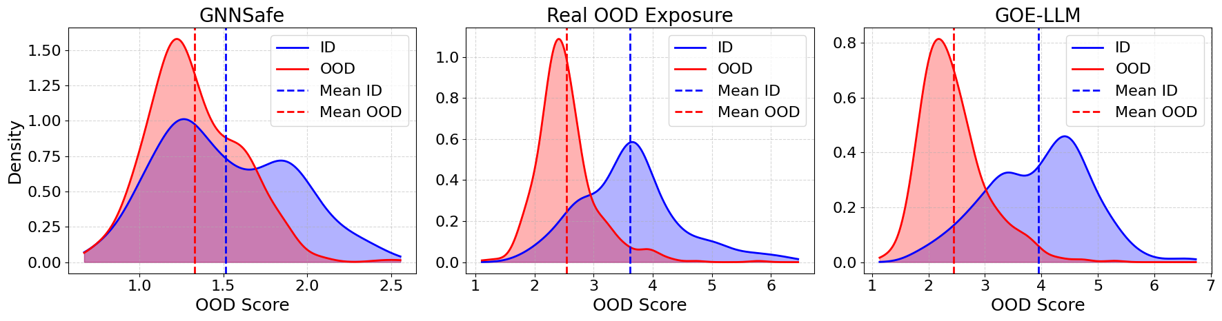
Figure 3: The OOD scores of GNNSafe, GNNSafe++ and GOE-LLM on Pubmed dataset.

Since there is no established graph-specific OOD detection benchmark that models real distributional shifts among nodes, most existing work on node-level graph OOD detection simply assumes that nodes from randomly selected classes are designated as OOD. However, this setting has notable limitations. For example, if the ID classes are more heterogeneous or closely resemble the OOD classes, the ID classifier may fail to learn a well-defined decision boundary, resulting in high softmax confidence scores for OOD nodes. Additionally, if the set of ID classes spans a broad and diverse range of features, the model may naturally assign high confidence to OOD nodes, violating the common assumption that OOD nodes should receive lower confidence scores. Therefore, using real or pseudo-OOD nodes can provide a more realistic and effective training signal for OOD detection. By explicitly exposing the model to samples that are semantically or structurally different from the ID distribution, we can help the classifier better distinguish between ID and OOD nodes. This leads to more calibrated confidence estimates and improved robustness under open-world scenarios.

To demonstrate this, we visualize the OOD scores on the Citeseer dataset for GNNSafe, GOE-LLM, and GNNSafe++. As shown in Fig. 3, compared to the method without OOD exposure, our approach assigns notably lower OOD scores to ID nodes and higher scores to OOD nodes, resulting in a more distinct separation between the two groups.

4.4 Zero-shot OOD Annotation

We present the zero-shot OOD detection performance of the LLM. The prompt we use for zero-shot OOD node identification is as follows:

As a research scientist, your task is to analyze and classify {object} based on their main topics, meanings, background, and methods.

Please first read the content of the {object} carefully. Then, identify the {object}’s key focus. Finally, match the content to one of the given categories:

[Category 1, Category 2, Category 3, ...]

Given the current possible categories, determine if it belongs to one of them. If so, specify that category; otherwise, say "none".

[Insert {Object} Content Here]

For each dataset, we prompt the LLM to determine whether each node in the test set belongs to one of the predefined ID categories. If not, the node is considered an OOD node. We then obtain binary OOD prediction results from the LLM and compute its accuracy. The results are shown in Table 2. We use accuracy as the sole evaluation metric for the LLM’s zero-shot OOD annotation performance, as the LLM cannot directly produce soft OOD scores (e.g., those defined in Eqn. 2). Instead, it only outputs hard binary predictions (0 or 1).

	Cora	Citeseer	Pubmed	Wiki-CS
Zero-shot OOD annotation	0.7190	0.7260	0.8410	0.7470

Table 2: Accuracy of using LLM to identify whether the unlabeled nodes are OOD nodes or not.

4.5 Synthetic Data Model

In this section, we combine labeled ID nodes and pseudo-OOD nodes to train the synthetic data models, as described in Section 3.5. Specifically, we randomly select $20\times K$ ID nodes and pseudo-OOD nodes annotated by the LLM. In this way, we use the same number of ID and OOD nodes to train the synthetic data models.

Table 3: Performance comparison (best highlighted in bold) of different synthetic data models on ID classification and OOD detection tasks.

Methods	Cora				Citeseer				Pubmed				Wiki-CS
	ACC $\uparrow$	AUROC $\uparrow$	AUPR $\uparrow$	FPR95 $\downarrow$	ACC $\uparrow$	AUROC $\uparrow$	AUPR $\uparrow$	FPR95 $\downarrow$	ACC $\uparrow$	AUROC $\uparrow$	AUPR $\uparrow$	FPR95 $\downarrow$	ACC $\uparrow$	AUROC $\uparrow$	AUPR $\uparrow$	FPR95 $\downarrow$
GOE-LLM	0.8780	0.9264	0.9233	0.3268	0.8444	0.8107	0.8082	0.7104	0.8636	0.8985	0.8955	0.5108	0.8764	0.9014	0.9212	0.7728
$(K+1)$-Classifier	0.8716	0.9138	0.9185	0.4224	0.8336	0.8189	0.8200	0.6648	0.8840	0.9060	0.8968	0.3980	0.8684	0.8015	0.7923	0.6648

For the first approach, we can add a binary classification layer on top of the output features of the ID classifier to predict the OOD score $z_{\text{ood}}=\mathbf{w}^{\top}\phi(x)$, where $\mathbf{w}\in\mathbb{R}^{h}$, and $x$ is the output of the hidden layer from the GNN-based ID classifier. The OOD score of node $v_{i}$ is then defined as $S_{\text{OOD}}(v_{i})=\sigma(z_{\text{ood}})$, where $\sigma(\cdot)$ denotes the sigmoid function. In the second approach, we train a $(K+1)$-class classifier and define the softmax probability of the $(K+1)$-th class as the OOD score. However, the performance of the first approach is not satisfactory in the current setting; therefore, we only report the results of the $(K+1)$-class classifier. The results are presented in Table 3. From the results, we observe that using Eqn. 3 to regularize the training of the ID classifier does not degrade ID classification performance. At the same time, it significantly improves OOD detection performance compared to the baselines. Furthermore, the $(K+1)$-class classifier generally achieves performance comparable to our regularization method.

4.6 How Many Synthetic OOD Nodes Do We Need?

In this section, we prompt the LLM to generate different numbers of pseudo-OOD nodes. The prompt used for OOD node generation is provided in Prompt 4.6.

Please generate {num_generated_samples} {object}(s) belonging to the category ’{category_name}’, including title and abstract.

Output Format:

• Title: <Generated Title>

• Abstract: <Generated Abstract>

	ID ACC $\uparrow$	AUROC $\uparrow$	AUPR $\uparrow$	FPR@95 $\downarrow$
No Exposure	0.8916	0.5954	0.6403	0.8928
2 OOD Nodes	0.8864	0.6692	0.6961	0.8708
3 OOD Nodes	0.8896	0.7401	0.7566	0.8100
5 OOD Nodes	0.8796	0.7674	0.7857	0.8036
10 OOD Nodes	0.8820	0.7908	0.8035	0.7780
20 OOD Nodes	0.8856	0.8043	0.8073	0.7400

Table 4: Performance comparison using different numbers of generated pseudo-OOD nodes for OOD exposure on the Pubmed dataset.

Table 4 presents the ID classification and OOD detection performance using different numbers of generated pseudo-OOD nodes. From the results, we can see that using more pseudo-OOD nodes improves OOD detection performance. When the number of generated OOD nodes reaches around 10, the performance nearly converges to a value that is significantly higher than that achieved without OOD exposure. This suggests that even a small number of pseudo-OOD nodes can provide meaningful OOD exposure during training, helping the model learn a more robust decision boundary between ID and OOD nodes. Moreover, it demonstrates the effectiveness of leveraging LLM-generated pseudo-OOD nodes as a lightweight and label-efficient alternative to relying on real OOD data. Another observation is that, among all cases, the ID classification accuracy is highest when no OOD exposure is performed. However, the degradation in ID classification performance is negligible when pseudo-OOD nodes are used to regularize the training of the ID classifier. This further demonstrates that the trade-off described in Section 3.2 is favorable, as pseudo-OOD exposure significantly improves OOD detection performance while having minimal impact on ID classification accuracy.

5 Conclusion

In this paper, we propose GOE-LLM, a novel framework for OOD detection on TAGs that removes the dependency on real OOD data through the use of LLMs. By designing two exposure strategies—LLM-based OOD identification and OOD node generation—we enable label-efficient, scalable, and effective OOD exposure. Extensive experiments across diverse datasets demonstrate that GOE-LLM achieves strong performance compared to methods relying on real OOD data, and significantly surpasses existing methods without OOD exposure. Future research could further explore the integration of more advanced prompting strategies to enhance the quality of pseudo-OOD samples. Additionally, investigating adaptive graph structure learning techniques tailored to generated nodes may yield further performance gains. Moreover, extending GOE-LLM to other graph learning tasks—such as graph-level OOD detection and OOD detection on dynamic TAGs—could be a promising direction.

Broader Impact This work paves the way for broader application of LLMs in graph learning tasks and highlights their potential in tackling distributional shifts in open-world graph settings.

Limitations While the proposed method significantly improves OOD detection performance on many graph datasets, it is only applicable to TAG datasets. For graphs without textual information, the proposed solution may no longer be effective, and more generalizable OOD exposure methods would need to be developed.

Appendix A ID and OOD Split

Table 5: ID classes and ID ratio for different datasets.

Dataset	ID class	ID ratio
Cora	[2, 4, 5, 6]	47.71%
Citeseer	[0, 1, 2]	55.62%
WikiCS	[1, 4, 5, 6]	38.79%
Pubmed	[0, 1]	60.75%

Appendix B Dataset Descriptions

Cora

The Cora dataset [11] contains 2,708 scientific publications categorized into seven research topics: case-based reasoning, genetic algorithms, neural networks, probabilistic methods, reinforcement learning, rule learning, and theory. Each node represents a paper, and edges correspond to citation links between papers, forming a graph with 5,429 edges.

CiteSeer

The CiteSeer dataset [5] consists of 3,186 scientific articles classified into six research domains: Agents, Machine Learning, Information Retrieval, Databases, Human-Computer Interaction, and Artificial Intelligence. Each node represents a paper, with node features extracted from the paper’s title and abstract. The graph is constructed based on citation relationships among the publications.

WikiCS

WikiCS [12] is a Wikipedia-based graph dataset constructed for benchmarking graph neural networks. Nodes correspond to articles in computer science, divided into ten subfields serving as classification labels. Edges represent hyperlinks between articles, and node features are derived from the corresponding article texts.

PubMed

The PubMed dataset [15] comprises scientific articles related to diabetes research, divided into three categories: experimental studies on mechanisms and treatments, research on Type 1 Diabetes with an autoimmune focus, and Type 2 Diabetes studies emphasizing insulin resistance and management. The citation graph connects related papers, with node features derived from medical abstracts.

Appendix C Evaluation Metrics

We use the following metrics to evaluate in-distribution (ID) classification and out-of-distribution (OOD) detection performance:

Accuracy (ACC)

Measures the proportion of correctly classified ID nodes:

$$\text{ACC}=\frac{1}{|\mathcal{D}_{\text{ID}}|}\sum_{x_{i}\in\mathcal{D}_{\text{ID}}}\mathbb{1}\left[\hat{y}_{i}=y_{i}\right],$$ (6)

where $\hat{y}_{i}$ is the predicted class label and $y_{i}$ is the true class label.

Area Under the ROC Curve (AUROC)

Evaluates how well the OOD detector ranks OOD nodes higher than ID nodes based on their OOD scores. It is defined as:

$$\text{AUROC}=\mathbb{P}\left(s_{\text{OOD}}(x_{\text{OOD}})>s_{\text{OOD}}(x_{\text{ID}})\right),$$ (7)

where $s_{\text{OOD}}(\cdot)$ denotes the OOD score function.

Area Under the Precision-Recall Curve (AUPR)

Measures the area under the curve defined by precision and recall:

Precision $$=\frac{\text{TP}}{\text{TP}+\text{FP}},$$ (8)

Recall $$=\frac{\text{TP}}{\text{TP}+\text{FN}},$$ (9)

AUPR $$=\int_{0}^{1}\text{Precision}(r)\,dr,$$ (10)

where OOD nodes are treated as the positive class, and $r$ denotes recall.

False Positive Rate at 95% True Positive Rate (FPR@95)

Indicates the fraction of ID samples incorrectly predicted as OOD when the true positive rate (TPR) on OOD samples is 95%:

$$\text{FPR@95}=\frac{\text{FP}_{\text{ID}}}{\text{FP}_{\text{ID}}+\text{TN}_{\text{ID}}}\Bigg{|}_{\text{TPR}=0.95},$$ (11)

where FP and TN are false positives and true negatives on ID data, respectively.

Appendix D Standard Deviation Results

Table 6: Standard deviation results for various models across ID classification and OOD detection metrics. All values are in percentages.

Model	Methods	Cora				Citeseer				Pubmed				Wiki-CS
		ACC	AUROC	AUPR	FPR95	ACC	AUROC	AUPR	FPR95	ACC	AUROC	AUPR	FPR95	ACC	AUROC	AUPR	FPR95
Baselines	MSP	2.46	1.90	1.47	7.68	1.39	2.85	3.04	5.38	3.06	2.12	3.02	2.37	2.73	3.65	4.19	6.74
	Entropy	2.18	2.78	1.87	8.91	1.39	2.59	2.80	6.31	3.06	2.12	3.02	2.37	2.71	3.33	3.71	7.10
	Energy	2.17	2.18	1.58	9.95	1.61	2.54	2.27	5.68	1.13	8.70	9.23	2.82	2.67	5.70	4.92	13.74
	GNNSafe	2.18	1.74	2.12	10.52	1.61	2.58	2.36	5.91	1.23	14.34	13.08	8.26	2.63	0.80	0.90	16.60
	GRASP	2.18	1.88	1.34	13.29	1.62	2.88	2.82	6.92	1.32	12.34	11.76	5.70	2.92	2.58	3.18	12.96
Ours	Identifier	2.53	0.88	1.42	2.24	1.65	2.01	1.85	7.66	2.03	2.48	3.02	7.69	2.20	0.90	1.26	11.86
	Generator	2.18	1.67	2.12	7.03	1.49	1.31	1.58	7.12	2.69	6.86	5.62	7.79	2.66	1.22	1.09	1.62
Real OOD	GNNSafe++	2.57	0.93	1.46	3.84	1.47	2.08	2.22	8.69	1.26	3.83	3.45	1.13	2.41	1.04	1.32	12.27

References

- [1] Momin Abbas, Muneeza Azmat, Raya Horesh, and Mikhail Yurochkin. Out-of-distribution detection using synthetic data generation. arXiv preprint arXiv:2502.03323, 2025.
- [2] Chentao Cao, Zhun Zhong, Zhanke Zhou, Yang Liu, Tongliang Liu, and Bo Han. Envisioning outlier exposure by large language models for out-of-distribution detection. arXiv preprint arXiv:2406.00806, 2024.
- [3] Xuefeng Du, Zhen Fang, Ilias Diakonikolas, and Yixuan Li. How does unlabeled data provably help out-of-distribution detection? arXiv preprint arXiv:2402.03502, 2024.
- [4] Xuefeng Du, Zhaoning Wang, Mu Cai, and Yixuan Li. Vos: Learning what you don’t know by virtual outlier synthesis. arXiv preprint arXiv:2202.01197, 2022.
- [5] C Lee Giles, Kurt D Bollacker, and Steve Lawrence. Citeseer: An automatic citation indexing system. In Proceedings of the third ACM conference on Digital libraries, pages 89–98, 1998.
- [6] Dan Hendrycks and Kevin Gimpel. A baseline for detecting misclassified and out-of-distribution examples in neural networks. arXiv preprint arXiv:1610.02136, 2016.
- [7] Dan Hendrycks, Andy Zou, Mantas Mazeika, Leonard Tang, Bo Li, Dawn Song, and Jacob Steinhardt. Pixmix: Dreamlike pictures comprehensively improve safety measures. In Proceedings of the IEEE/CVF Conference on Computer Vision and Pattern Recognition, pages 16783–16792, 2022.
- [8] Nathan A Inkawhich, Eric K Davis, Matthew J Inkawhich, Uttam K Majumder, and Yiran Chen. Training sar-atr models for reliable operation in open-world environments. IEEE Journal of Selected Topics in Applied Earth Observations and Remote Sensing, 14:3954–3966, 2021.
- [9] Weitang Liu, Xiaoyun Wang, John Owens, and Yixuan Li. Energy-based out-of-distribution detection. Advances in neural information processing systems, 33:21464–21475, 2020.
- [10] Longfei Ma, Yiyou Sun, Kaize Ding, Zemin Liu, and Fei Wu. Revisiting score propagation in graph out-of-distribution detection. In The Thirty-eighth Annual Conference on Neural Information Processing Systems.
- [11] Andrew Kachites McCallum, Kamal Nigam, Jason Rennie, and Kristie Seymore. Automating the construction of internet portals with machine learning. Information Retrieval, 3:127–163, 2000.
- [12] Péter Mernyei and Cătălina Cangea. Wiki-cs: A wikipedia-based benchmark for graph neural networks. arXiv preprint arXiv:2007.02901, 2020.
- [13] Aristotelis-Angelos Papadopoulos, Mohammad Reza Rajati, Nazim Shaikh, and Jiamian Wang. Outlier exposure with confidence control for out-of-distribution detection. Neurocomputing, 441:138–150, 2021.
- [14] N Reimers. Sentence-bert: Sentence embeddings using siamese bert-networks. arXiv preprint arXiv:1908.10084, 2019.
- [15] Prithviraj Sen, Galileo Namata, Mustafa Bilgic, Lise Getoor, Brian Galligher, and Tina Eliassi-Rad. Collective classification in network data. AI magazine, 29(3):93–93, 2008.
- [16] Yu Song and Donglin Wang. Learning on graphs with out-of-distribution nodes. In Proceedings of the 28th ACM SIGKDD Conference on Knowledge Discovery and Data Mining, pages 1635–1645, 2022.
- [17] Leitian Tao, Xuefeng Du, Xiaojin Zhu, and Yixuan Li. Non-parametric outlier synthesis. arXiv preprint arXiv:2303.02966, 2023.
- [18] Sachin Vernekar, Ashish Gaurav, Vahdat Abdelzad, Taylor Denouden, Rick Salay, and Krzysztof Czarnecki. Out-of-distribution detection in classifiers via generation. arXiv preprint arXiv:1910.04241, 2019.
- [19] Ziyu Wang, Bin Dai, David Wipf, and Jun Zhu. Further analysis of outlier detection with deep generative models. Advances in Neural Information Processing Systems, 33:8982–8992, 2020.
- [20] Qitian Wu, Yiting Chen, Chenxiao Yang, and Junchi Yan. Energy-based out-of-distribution detection for graph neural networks. arXiv preprint arXiv:2302.02914, 2023.
- [21] Zhiping Xiao, Weiping Song, Haoyan Xu, Zhicheng Ren, and Yizhou Sun. Timme: Twitter ideology-detection via multi-task multi-relational embedding. In Proceedings of the 26th ACM SIGKDD international conference on knowledge discovery & data mining, pages 2258–2268, 2020.
- [22] Haoyan Xu, Runjian Chen, Yueyang Wang, Ziheng Duan, and Jie Feng. Cosimgnn: towards large-scale graph similarity computation. arXiv preprint arXiv:2005.07115, 2020.
- [23] Haoyan Xu, Ziheng Duan, Yueyang Wang, Jie Feng, Runjian Chen, Qianru Zhang, and Zhongbin Xu. Graph partitioning and graph neural network based hierarchical graph matching for graph similarity computation. Neurocomputing, 439:348–362, 2021.
- [24] Haoyan Xu, Kay Liu, Zhengtao Yao, Philip S Yu, Kaize Ding, and Yue Zhao. Lego-learn: Label-efficient graph open-set learning. arXiv preprint arXiv:2410.16386, 2024.
- [25] Haoyan Xu, Zhengtao Yao, Yushun Dong, Ziyi Wang, Ryan A Rossi, Mengyuan Li, and Yue Zhao. Few-shot graph out-of-distribution detection with llms. arXiv preprint arXiv:2503.22097, 2025.
- [26] Hao Yan, Chaozhuo Li, Ruosong Long, Chao Yan, Jianan Zhao, Wenwen Zhuang, Jun Yin, Peiyan Zhang, Weihao Han, Hao Sun, et al. A comprehensive study on text-attributed graphs: Benchmarking and rethinking. Advances in Neural Information Processing Systems, 36:17238–17264, 2023.
- [27] Jingkang Yang, Kaiyang Zhou, Yixuan Li, and Ziwei Liu. Generalized out-of-distribution detection: A survey. International Journal of Computer Vision, 132(12):5635–5662, 2024.
- [28] Junhan Yang, Zheng Liu, Shitao Xiao, Chaozhuo Li, Defu Lian, Sanjay Agrawal, Amit Singh, Guangzhong Sun, and Xing Xie. Graphformers: Gnn-nested transformers for representation learning on textual graph. Advances in Neural Information Processing Systems, 34:28798–28810, 2021.
- [29] Jingyang Zhang, Nathan Inkawhich, Randolph Linderman, Yiran Chen, and Hai Li. Mixture outlier exposure: Towards out-of-distribution detection in fine-grained environments. In Proceedings of the IEEE/CVF Winter Conference on Applications of Computer Vision, pages 5531–5540, 2023.
- [30] Xujiang Zhao, Feng Chen, Shu Hu, and Jin-Hee Cho. Uncertainty aware semi-supervised learning on graph data. Advances in neural information processing systems, 33:12827–12836, 2020.
- [31] Yanqiao Zhu, Yuanqi Du, Yinkai Wang, Yichen Xu, Jieyu Zhang, Qiang Liu, and Shu Wu. A survey on deep graph generation: Methods and applications. In Learning on Graphs Conference, pages 47–1. PMLR, 2022.