Big-Bang nucleosynthesis constraints on (dual) Kaniadakis cosmology
Abstract
We investigate the concept of Kaniadakis entropy and its dual formulation, examining their implications for gravitational dynamics within the framework where gravity emerges as an entropic force resulting from changes in the informational content of a physical system. In this context, we derive a modified form of Newton’s law of gravitation that reflects the corrections introduced by both Kaniadakis entropy and its dual state. Furthermore, we apply the emergent gravity scenario at large scales and derive the modified Friedmann equations incorporating corrections from (dual) Kaniadakis entropy. Our results provide deeper insights into the interplay between thermodynamics and gravitational dynamics. In order to constrain the model parameter, we study the Big-Bang Nucleosynthesis in the context of (dual) Kaniadakis cosmology. We explore an alternative method to establish limits on the Kaniadakis parameter, denoted as , by examining how (dual) Kaniadakis cosmology influences the primordial abundances of light elements i.e. Helium , Deuterium and Lithium . Our analysis indicates that the obtained ranges for the dual Kaniadakis parameter (unlike the Kaniadakis parameter) exhibit overlap for the aforementioned light elements, and the allowed values fall within the range , which shows that the deviations from the conventional Bekenstein-Hawking formula are minimal, as expected. This consistency between the ranges suggests a potential solution to the well-known Lithium problem. Furthermore, we discuss the relationship between cosmic time and temperature within the framework of (dual) Kaniadakis cosmology. We observe that an increase in the Kaniadakis parameter leads to a rise in the temperature of the early universe. Conversely, when the dual Kaniadakis parameter increases, the temperature of the early universe decreases.
I Introduction
Black hole thermodynamics suggests that gravitational field equations, such as Einstein’s general relativity, could emerge from fundamental thermodynamic principles. This conjecture is founded on the profound relationship between thermodynamic quantities such as entropy and temperature and the geometric properties of the horizon, including its area and surface gravity. The evidence for the thermodynamic-gravity correspondence is multifaceted. At its core is the realization that Einstein’s field equations can be derived from the fundamental thermodynamic relation when applied to local horizons. This derivation, first achieved by Jacobson Jac , extended beyond Einstein’s gravity to encompass gravity Elin , Gauss-Bonnet gravity, scalar-tensor gravity, and the more general Lovelock gravity Pad1 ; Pad2 ; Cai1 ; Pad3 . In cosmological contexts, this connection becomes particularly striking. In the context of Friedmann-Robertson-Walker (FRW) cosmology, it has been shown that the first Friedmann equation, when applied at the apparent horizon, is directly related to the first law of thermodynamics, expressed as . This relationship works both ways wang1 ; wang2 ; CaiKim ; Cai2 ; Shey11 ; Shey22 ; Shey3 ; Shey4 . The connection between thermodynamic principles at the boundary and gravitational field equations in the bulk is crucial for understanding the holographic principle. The thermodynamic view of gravity is further supported by ideas from statistical mechanics. Verlinde’s theory of entropic gravity Ver demonstrated that gravity can emerge from fundamental principles such as the holographic principle and the equipartition law of energy, specifically applied to the degrees of freedom at the horizon. In this framework, variations in the system’s information content lead to the generation of an entropic force, which can be expressed mathematically by the gravitational field equations. This suggests that gravity may not be a fundamental force but rather an emergent phenomenon resulting from the statistical properties of the underlying system. The entropic nature of gravity has been thoroughly investigated (see, for example, Cai3 ; sheyECFE ; Visser ; SRM and the references therein). The most profound implication comes from Padmanabhan’s work on emergent gravity, which proposes expansion of the universe can be understood as a consequence of space emerging itself PadEm . In this concept, cosmic space develops as cosmic time advances. The core ideas in this framework are the degrees of freedom of matter fields in both the bulk and on the boundary, with both playing a significant role. By determining the difference in degrees of freedom between the boundary and the bulk and equating it to the change in volume, the Friedmann equations can be derived CaiEm ; Yang ; Sheyem .
It is essential to emphasize that, all discussed approaches share one crucial feature: the entropy expression fundamentally shapes how gravitational field equations emerge from thermodynamics. Modify the entropy, and you necessarily modify the gravitational theory CaiLM ; SheT1 ; Odin1 ; SheT2 ; Emm2 ; SheB1 ; SheB2 ; Odin2 ; Odin3 ; Odin4 ; Odin5 .
In the present work, by applying the (dual) Kaniadakis entropy formalism to horizon thermodynamics, we derive and analyze the resulting modifications to cosmological field equations. Previous studies Lym ; Shey1 ; Shey2 have examined the role of Kaniadakis entropy, in cosmological frameworks. The analysis in Lym explored how Kaniadakis entropy modifies cosmology by examining the energy exchange at the universe’s apparent horizon. Their approach was based on the fundamental thermodynamic relation , where the , represents the outward energy flux across the horizon over an infinitesimal time interval. This formulation demonstrated that the modified Friedmann equations acquire additional terms, which can be interpreted as an effective dark energy component influenced by the Kaniadakis parameter Lym . While Lym studied entropy effects through energy fluxes, the authors of Refs. Shey1 ; Shey2 took a geometrically focused approach, modifying only the left-hand side of the field equations. This distinction is crucial because: entropy fundamentally originates from the geometric properties of spacetime. Moreover, considering the universe’s expansion, the work term related to volume change should be included in the first law of thermodynamics, formulated as Shey1 ; Shey2 . Our work differs from Lym ; Shey1 ; Shey2 in that they derived modified Friedmann equations using the first law of thermodynamics with Kaniadakis entropy, while here we work in the framework of entropic force and emergent gravity and by incorporating both Kaniadakis and dual Kaniadakis entropy correction terms. Our approach provides a new perspective on the effects of generalized entropy corrections in cosmology and their influence on gravitational dynamics.
On the other side, Big-Bang Nucleosynthesis (BBN) is a process that occurred in the early universe shortly after the Big-Bang, during a time when the universe was extremely hot and dense. This process took place approximately between seconds and a few hundred seconds (around minutes) after the Big-Bang. During BBN, the high temperature enabled nuclear reactions, resulting in the formation of light elements such as Helium , Deuterium and Lithium . As the universe expanded and cooled, the nuclear reactions gradually slowed and finally ceased, leading to the observed amounts of these light elements that we observe in the universe today. It is well-known that both BBN and the Cosmic Microwave Background (CMB) radiation serve as strong evidences that our universe was once extremely hot and dense in its early stages.
The theory of BBN imposes strict constraints on various cosmological models, requiring consistency between theoretical predictions and observational data. Modified cosmological models can influence the primordial abundances of these light elements Anish . While standard BBN theory effectively accounts for the observed amounts of helium and hydrogen, it faces challenges with Lithium, leading to the so-called cosmological Lithium problem. This issue is a significant topic of discussion in modern cosmology, and researchers are interested in whether it can be resolved within modified cosmological frameworks. The aim is to investigate the cosmological Lithium problem within the context of modified cosmology, specifically looking at how certain values of model parameters might alleviate the issue.
Our aim in this work is to explore the implications of (dual) Kaniadakis cosmology on BBN and derive constraints on both Kaniadakis () and dual Kaniadakis () parameters. In this context, we can evaluate the feasibility of (dual) Kaniadakis cosmology by applying the conditions of BBN. The main difference between this work and the work presented in the Luciv , is that in this paper we constrain the Kaniadakis parameter and its dual (deformed) state using the available observational data for the abundances of the light elements helium, deuterium, and Lithium, and we examine the Lithium problem within the framework of (dual) Kaniadakis cosmology. Another key difference in our work is that for constraining the Kaniadakis parameter and its dual parameter, we use the Friedmann equation derived from the emergent gravity approach, whose sign and coefficient of the correction term differ from those obtained via the first law of thermodynamics, which leads to different results for BBN constraints. Additionally, we will examine the relationship between cosmic time and temperature in the early universe, particularly in the framework of modified (dual) Kaniadakis cosmology, which is a topic that has not been previously addressed in the literatures. Our analysis shows that the early universe becomes hotter with an increase in the Kaniadakis parameter, while an increase in the dual Kaniadakis parameter results in a decrease in the temperature of early universe.
This paper is structured as follows. Section II presents a comprehensive overview of (dual) Kaniadakis entropy’s theoretical foundations and its implications for black hole thermodynamics and MOND theory. In section III, we utilize the entropic force framework to derive the modified Friedmann equations. In section IV, we employ the concept of emergent gravity to derive the modified Friedmann equations. In section V, we constrain both Kaniadakis and dual Kaniadakis parameters using BBN data within the framework of (dual) Kaniadakis cosmology. Section VI then establishes the time-temperature relation in this cosmological model. Finally, we conclude with closing remarks in section VII.
II Modified (Dual) Kaniadakis entropy
Let us start with reviewing the origin of the Kaniadakis entropy. Kaniadakis entropy is the generalization of Boltzmann-Gibbs-Shannon entropy which contains one new parameter. It has been argued that the Kaniadakis entropy can be expressed as Kan1 ; Kan2 ; Abreu:2016avj ; Abreu:2017fhw ; Abreu:2017hiy ; Abreu:2018mti ; Yang:2020ria ; Abreu:2021avp
| (1) |
where denotes the probability in which the system to be in a specific microstate , and represents the total number of the system configurations. Here is called the Kaniadakis parameter which is a dimensionless parameter ranges as , and measures the deviation from standard statistical mechanics. For simplicity, hereafter we set .
One may apply the Kaniadakis entropy to the black hole thermodynamics. For this purpose, one proposes , and , where is the usual black hole entropy. Thus, we have Mor
| (2) |
Substituting expression (2) into Eq. (1), after some calculations, we find the Kaniadakis entropy versus black hole entropy as,
| (3) |
If we expand expression (3) for , we arrive at
| (4) |
When , the standard entropy is restored. Alternatively, one may assume the entropy of the black hole as AbreuNet1
| (5) |
Solving this equation for , one finds
| (6) |
In order to have a correct limiting BG entropy, we choose the positive sign in the above relation. Now we define the dual (deformed) Kaniadakis entropy as AbreuNet1 ; Amb
| (7) |
where , with is the horizon area. When , one recovers , as expected.
It was shown that the dual Kaniadakis entropy (7) can provide a theoretical origin for the MOND theory Amb . MOND theory success comes from its ability to explain galaxy rotation curves by adjusting Newton’s second law, offering a different formulation for force as Milgrom1
| (8) |
where represents the usual acceleration, is a characteristic constant, and is a function behaves as and To determine a specific functional form for based on entropic considerations, we begin with a thermodynamically effective gravitational force equation as sheyECFE
| (9) |
In this framework, represents the area of the holographic screen, and characterizes its entropy. The generality of Eq. (9) means it holds for any valid entropy function. As an illustration, by using the Bekenstein-Hawking entropy formula in this Equation, the standard Newtonian gravitational force is recovered. It has been shown that when in Eq. (9), dual Kaniadakis modified entropy is adopted instead of , one can derive the MOND theory Amb . Let first take derivative of Eq. (7) to find
| (10) |
Where . Combining with Eq. (9), we find the effective gravitational force as
| (11) | |||||
where and . Based on this equation, the interpolating function is realized as
| (12) |
which implies . Clearly, this interpolating function satisfies the conditions for . Therefore, when dual Kaniadakis modified entropy given in Eq. (7) is combined with the effective force expression Eq. (9), the resulting model mirrors MOND theory including its distinctive transition function Eq. (12), which is precisely the standard interpolating function used in MOND theory Begeman ; Gentile .
Note that expression (7) can be also rewritten as
| (13) |
If we expand expression (13) for , we arrive at
| (14) |
The first term is the usual area law of black hole entropy, while the second term is the leading order Kaniadakis correction term. It is clear that the leading order term for dual (deformed) Kaniadakis entropy has a negative sign.
In summary, for (dual) Kaniadakis entropy, the modified entropy expression, up to the first order correction term, can be written as
| (15) |
where and stands, respectively, for the Kaniadakis and dual Kaniadakis entropy and we have dropped the star for dual Kaniadakis entropy.
III Kaniadakis entropic corrections to Newton’s law and Friedmann equations
This section explores entropic gravity principles, using entropy expression (15) to develop correction terms for Newton’s gravitational law and modifications to the Friedmann equations. According to Verlinde’s framework Ver , gravitational effects arise as material bodies alter information entropy due to their relative motion with respect to holographic screens. In this framework, the entropic force satisfies the relation
| (16) |
for test particle displacements. Here, represents the displacement of a particle from the holographic screen, while denotes the temperature and corresponds to the change in entropy on the screen. We study a configuration where a spherical mass is enclosed by a surface , and a test particle of mass is placed adjacent to , at a distance smaller than its reduced Compton wavelength , ensuring that remains the boundary separating the two masses. For a test mass displaced by from the surface , the variation of entropy (15) takes the form
| (17) |
The area of the surface is given by , and the total energy enclosed within this surface is . The surface contains discrete information units ”bytes” whose quantity scales with surface area according to , where is the total byte count and is a fundamental constant. Since , any change in the area satisfies . According to the equipartition law of energy, the temperature is related to the total energy on the surface is given by
| (18) |
Where we have set . Using relation , we can rewrite Eq. (18) as
| (19) |
By substituting Eqs. (17) and (19) into Eq. (16), we obtain
| (20) |
where . We can express the modified Newton’s law of gravity by defining . The result is
| (21) |
This is the modified Newton’s law of gravitation inspired by (dual) Kaniadakis corrections to entropy. Note that here and corresponds to the Kaniadakis and dual Kaniadakis modified entropy, respectively. In the limiting case where , the parameter vanishes, and the standard Newton’s law of gravitation is recovered.
Now we are going to derive the correction to the Friedmann equations. For this purpose, we consider a universe that is spatially homogeneous and isotropic, described by the line elements
| (22) |
where , and . The two-dimensional metric is given by =diag , where corresponds to open, flat, and closed universes, respectively. The apparent horizon, which serves as a natural boundary based on thermodynamic considerations, has a radius given by Cai2
| (23) |
where the Hubble parameter is given by . We model the matter and energy content of the universe as a perfect fluid, described by the energy-momentum tensor, where is the energy density and is the pressure. Since there is no observed energy exchange between the universe and any external environment, the local conservation of energy-momentum must hold . This condition guarantees that the total energy and momentum of the cosmic fluid remain dynamically conserved and leads to the continuity equation as
| (24) |
By applying Newton’s second law to a test particle near the surface and incorporating the gravitational force given by Eq. (21), we arrive at
| (25) |
The matter inside the spherical volume , has an energy density given by . Therefore, we have . By using this relation and , Eq. (25) can be reformulated as
| (26) |
This is the modified dynamical equation for Newtonian cosmology, incorporating the Kaniadakis (dual Kaniadakis) entropy correction. From another perspective, we define the active gravitational mass following Cai3 as
| (27) |
Now, in the expression for , is replaced by in Eq. (26). The result is
| (28) |
If we multiply both sides of Eq. (28) by factor and applying the continuity equation (24), we obtain the result after integration
| (29) |
Here, is an integration constant that can be interpreted as the curvature parameter. To evaluate the integral explicitly, we first solve the continuity equation (24), which has a solution
| (30) |
Where represents the equation of state parameter, and denotes the present energy density. Substituting Eq. (30) into Eq. (29) and performing the necessary calculations, we arrive at the expression
| (31) |
where and it is obtained based on Eq. (23). It is convenient to rewrite the above equation in a simplified form as
| (32) |
where the and , respectively, correspond to Kaniadakis and dual Kanidakis entropy. In the limiting case the standard Friedmann equation is recovered.
IV Corrections to Friedmann equations from emergence scenario
This section applies Padmanabhan’s gravity emergence paradigm PadEm to derive modified Friedmann equations, incorporating the adjusted entropy relation from Eq. (15). As previously mentioned in Padmanabhan’s proposal, the expansion of the universe is driven by the difference between degrees of freedom on the horizon and in the bulk. This idea will be further explored in the following sections. He expressed this idea mathematically as PadEm
| (33) |
where and represent the degrees of freedom on the boundary and in the bulk, respectively. In the case of a nonflat universe, this relation needs to be generalized, as suggested in Sheyem , leading to
| (34) |
where denotes the apparent horizon radius based on Eq. (23). The temperature corresponding to the apparent horizon is assumed to be
| (35) |
To express the number of degrees of freedom on the horizon, we use relation in which represents the entropy of the horizon. Thus, considering Eq. (15), we can identify
| (36) |
Where we have considered as the boundary area. Thus, we have
| (37) |
where and the positive sign corresponds to the entropy correction inspired by Kaniadakis, while the negative sign arises from the dual formulation. The total energy within the apparent horizon is expressed as the Komar energy, given by
| (38) |
where represents the volume of the sphere enclosed by the apparent horizon. Using the energy equipartition theorem, one derives the count of degrees of freedom for the bulk matter field as
| (39) |
This equation can be written as
| (40) |
assuming that in an expanding universe. By merging relations (37) and (40) with Eq. (34), we arrive at
| (41) |
After simplifying, we have
| (42) |
Now, by multiplying both sides by factor and using the continuity equation (24), we find
| (43) |
We can perform the integration of the above equation, which leads to the following result
| (44) |
By defining and using Eq. (23), we arrive at
| (45) |
where . This result matches the one derived from the entropic force in Eq. (32). Note that the is obtained by considering Kaniadakis entropy, and the is obtained from its dual entropy. In the limit , the Friedmann equation returns to its standard form.
V Constraints on Kaniadakis and Dual Kaniadakis parameters from BBN
V.1 Big Bang nucleosynthesis in (dual) Kaniadakis cosmology
In this section we first analyze the Kaniadakis cosmology during the radiation dominated epoch, and after that explore the BBN in the framework of (dual) Kaniadakis cosmology. Using Eq. (45), the modified Friedmann equation inspired by (dual) Kaniadakis entropy in the flat universe () can be written as
| (46) |
By defining and multiplying Eq. (46) by , the above equation can be rewritten as follows
| (47) |
Solving the above equation for and substituting in terms of , the following expression for the Hubble parameter is obtained
| (48) |
where and sign refer to the Kaniadakis entropy and the dual Kaniadakis entropy, respectively, while stands for the Hubble function in the standard cosmology. Since is small enough, we can expand the above expression and obtain the modified Hubble parameter as
| (49) |
We can rewrite the modified Hubble parameter (49) in the form
| (50) |
where the amplification factor is defined as
| (51) |
Substituting the energy density of relativistic particles, expressed as ( is the effective number of degrees of freedom and is the temperature), , reduced Planck mass Luciv , and into Eq. (V.1), we determine the amplification factor as
| (52) |
where the sign arises from the Kaniadakis cosmology, while the sign comes from its corresponding dual cosmology. Consistent with expectations, when , the amplification factor reduces to , and the general relativity (GR) limit is recovered.
V.2 Primordial light elements , D and Li in (dual) Kaniadakis cosmology
Next we explore constraints on the Kaniadakis parameter and dual Kaniadakis parameter, , by examining how (dual) Kaniadakis cosmology influences the primordial abundances of light elements, specifically Deuterium , Tritium , and Helium . By comparing theoretical predictions with observational data on these elements abundances, we derive bounds on and . The main idea is to replace the modified amplification factor found in (52) instead of the standard Z-factor that is associated with the effective number of neutrino species in Luciano . In the standard cosmological model, the parameter is equal to unity. However, if we consider modifications to gravity or the introduction of additional light particles, such as neutrinos, may differ from unity. In such scenarios, the modified Z-factor would be represented in the form Anish ; Luciano ; Boran
| (53) |
where in this context, represents the number of neutrino species. The baryon-antibaryon asymmetry , plays an important role in our analysis Adv ; Simha . Since we aim to focus on the effects of Kaniadakis cosmology on BBN, we set , ensuring that any deviation of from unity arises solely from the effects of Kaniadakis cosmology on BBN, not from additional particle degrees of freedom.
In the subsequent analysis, we adopt the approach outlined in Anish ; Sahoo and summarize its key aspects as:
(i) abundance-the production of begins when a proton and neutron combine to form . Subsequently, Deuterium transforms into Tritium and through the following processes
| (54) | ||||
| (55) | ||||
| (56) |
The final production of Helium occurs through the following nuclear reactions
| (57) |
The numerical best-fit analysis yields the following constraint for the primordial abundance Kneller ; Annu
| (58) |
In our analysis, follows from Eq. (52), with the baryon density parameter defined as Adv ; Simha
| (59) |
where the baryon to photon ratio is defined as Wamp . By setting , we arrive at the standard prediction from BBN for the abundance of , which is approximatively . Additionally, the observational data regarding the abundance of , along with the assumption that suggests that Brain . Consistency between previously mentioned value of and Eq. (58) indicates
| (60) |
So we can define the value of as
| (61) |
(ii) abundance- Deuterium forms via the process . In a similar manner, the Deuterium abundance can be calculated from the numerical best fit of Adv . It gives
| (62) |
As in the previous case, setting and reproduces the standard GR result . By equating the observed Deuterium abundance constraint Brain , with Eq. (62), we derive
| (63) |
Consequently, the parameter is constrained to
| (64) |
which exhibits partial overlap with the constraint from abundance of in relation (61).
(iii) abundance - the parameter given in Eq. (59) successfully reproduces the observed abundances of , and other light elements, yet it exhibits a tension with the measured abundance. In fact, the predicted abundance ratio of in the standard cosmological model compared to the observed Lithium abundance falls within the following range Boran
Quite unexpectedly, no current nucleosynthesis scenario, including standard BBN or its modifications, can explain low observed abundance of . This discrepancy is commonly known as cosmological Lithium problem Boran . By imposing consistency between observational values of Lithium abundance Brain , and the following numerical best fit for the abundance of
| (65) |
we can derive as
| (66) |
This restriction does not coincide with the findings regarding the abundance of , in Eq. (64), and abundance, in Eq.(61).
V.3 Discussion in the results
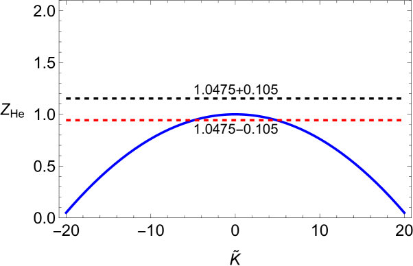
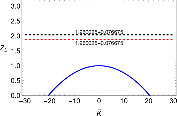
Here we discuss the obtained results, deriving the bound on both the Kaniadakis and dual Kaniadakis parameters. In Fig. 1 we plot relation (52) taking into account the sign, using the bounds presented in relation (61). As we can see, from the observational constraints on Helium abundance, the rescaled Kaniadakis parameter is constrained to the range
| (67) |
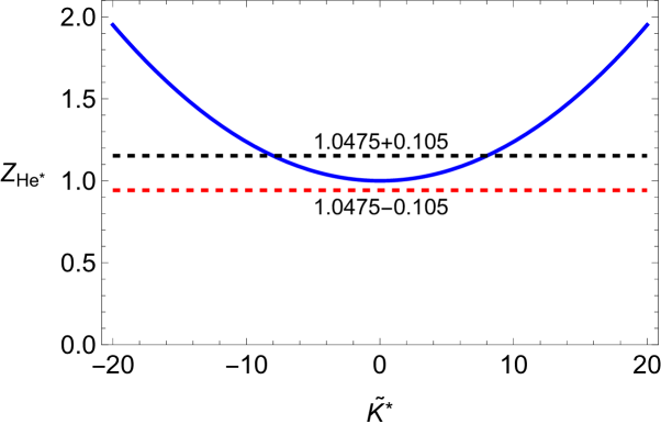
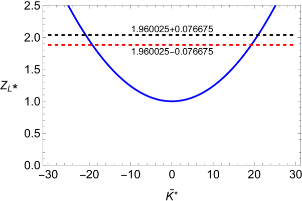
The results for the dual Kaniadakis parameter are shown in the Fig. 2. We observe that the dual Kaniadakis parameter lies in the range
| (68) |
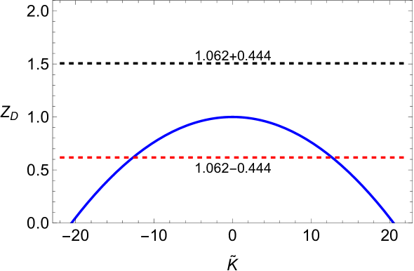
We have shown the results for Deuterium (using Eq. (64) and taking into account the sign in (52)) in Fig. 3. We observe that the corresponding range of Kaniadakis parameter is
| (69) |
Let us note that the allowed range of from Deuterium (69) is consistent with that obtained from given by (67).
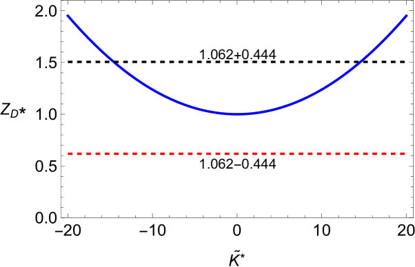
The results for the dual Kaniadakis parameter are shown in the Fig. 4. It is seen that the dual Kaniadakis parameter ranges as
| (70) |
We observe that the allowed range of from Deuterium (70) is consistent with that obtained from given by (68).
In the case of Lithium, as we can see in Fig. 5, the results obtained from primordial Lithium abundance do not provide a constrained range for the Kaniadakis parameter.
The results for the dual Kaniadakis parameter are shown in Fig. 6. The plot demonstrates that the range of for overlaps with the constraints on that and abundances provided in Eqs. (68) and (70).
| (71) |
Therefore, the allowed range for the dual Kaniadakis parameter, based on the observed light elements abundances, is the overlapping region of the intervals (68), (70) and (71), and hence the acceptable values for the dual Kaniadakis parameter are given by relation (68). Consistent with predictions, the deviation from standard Bekenestein-Hawking expression is small.
VI Time-Temperature relation in (Dual) Kaniadakis Cosmology
In this section, we derive the relation between time and temperature in the framework of (dual) Kaniadakis cosmology. Modifications to the Friedmann equations influence the thermodynamics of the early universe, leading to a different relation between time and temperature compared to the standard cosmological model. The state of thermal equilibrium in the early universe leads to the conservation of entropy within a co-moving volume Weinberg
| (72) |
Calculating the first derivative of the above equation with respect to time results
| (73) |
Substituting into the previous equation, we obtain
| (74) |
where can be reexpressed in the following manner
| (75) |
Integrating (75) with respect to temperature, the cosmic time can be obtained as
| (76) |
where the prime symbol indicates a derivative with respect to the temperature .
Specifically, during any era in which the primary component of the universe is a highly relativistic ideal gas, the entropy and energy densities are given by the following equations Weinberg
| (77) | |||||
| (78) |
where represents the total number of particles and antiparticles, considering each spin state individually Weinberg . By expanding and substituting , we derive the following result
| (79) |
Using as well as expression from Eq. (78), we reach
| (80) |
where we have defined . Integrating yields
| (81) |
where and signs refer to the Kaniadakis entropy and the dual Kaniadakis entropy, respectively. The above equation describes how cosmic time is connected to temperature in the context of (dual) Kaniadakis cosmology. In the limiting case where we have and GR is recovered Weinberg .
We have used the modified Friedmann equation which was derived in natural units where . However, the right hand side of Eq. (81) must have the dimensions of time, hence if we take into account all the constants in deriving the modified Friedmann equations and include all physical constants properly to ensure dimensional consistency, the constant takes the form
| (82) |
where we have defined
| (83) |
As a result, the right side of Eq. (81) is obtained in terms of time. In the early stages of the universe, the fundamental components included photons, three types of neutrinos, three types of antineutrinos, along with electrons and positrons. Under these conditions, the effective number of relativistic degrees of freedom is given by . Thus, Eq. (81) yields, in cgs (centimeter-gram-second) units,
| (84) |
where we have defined
| (85) |
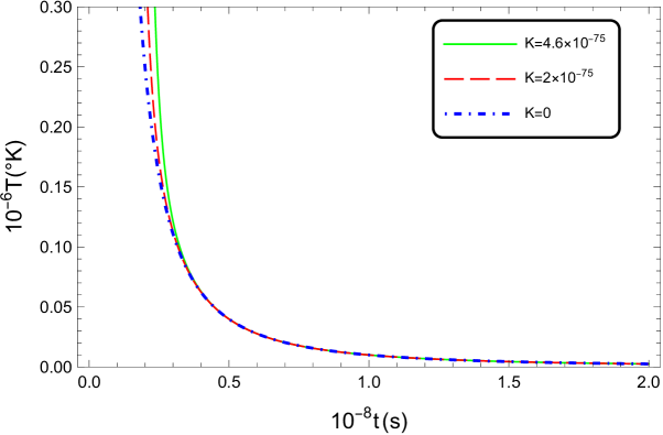
Here the sign arises from the Kaniadakis entropy, while the sign comes from dual Kaniadakis entropy. Again for we have and the result of GR is restored Weinberg . In Fig. 7, we plot the behavior of temperature as a function of cosmic time for different values of . We observe that as the Kaniadakis parameter increases, the temperature of the early universe increases, too.
The results for the relation between time and temperature in dual Kaniadakis cosmology are shown in Fig. 8. It is seen that as the dual Kaniadakis parameter increases, the temperature of the early universe decreases.
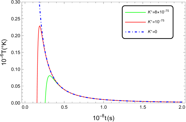
Let us note that for and negative sign in (dual Kaniadakis), Eq. (84) admits an extremum, and the time-temperature function in the dual Kaniadakis entropy framework has a relative maximum at (see Fig. 8). It is also clear that the dual Kaniadakis entropy model does not work well for the very early universe where . The physical reasons behind this behaviour of temperature in case of the (dual) Kaniadakis may be due to the effects of non-extensive thermodynamics. In standard cosmological model, both energy density and entropy follow the usual extensive thermodynamics. Kaniadakis cosmology represents non-extensivity, which leads to more significant interactions and correlations between particles. This results in an increased energy density for a given temperature, effectively requiring a higher temperature to fit the same energy density as in the GR case. The other reason can be the modification of Friedmann equations which leads to modification in expansion rate of the early universe. The larger values of Kaniadakis parameter leads to a slower expansion rate at very early universe, allowing more time for thermalization at higher temperatures. This behavior is consistent with other non-extensive thermodynamics frameworks (e. g., Tsalis cosmology), where deformation parameters usually results in high-energy effects.
VII Closing remarks
In this work, we have analyzed how Kaniadakis entropy and its dual form influence gravitational interactions. By applying these entropy measures within the entropic force framework, we first obtained the modified form of the Newton’s law of gravitation. We then extended our analysis to the relativistic regime, by deriving the modified Friedmann equations that govern cosmic evolution. Furthermore, we derived the modified Friedmann equations by establishing an equivalence between the difference in the degrees of freedom on the boundary and in the bulk, and the variation of the system’s volume. This approach, based on the emergent gravity scenario, incorporates entropy corrections and provides deeper insights into cosmic evolution. Thus, by incorporating (dual) Kaniadakis entropy, we have derived the modified Friedmann equation through a different theoretical approach. The final results are expressed in Eqs. (32) and (45) where the positive correction term originates from Kaniadakis entropy, while the negative correction term arises from its dual formulation.
We have used BBN data in order to find the bounds on the free parameter of (dual) Kaniadakis entropy. As we mentioned, (dual) Kaniadakis entropy introduces additional terms into the modified Friedmann equations. For consistency with BBN, these corrections must be sufficiently small. In order to impose bounds on the free parameters of the models, we explored the consequences of (dual) Kaniadakis cosmology on the primordial light elements formation. The analysis of light elements , and shows that the allowed ranges obtained for the dual Kaniadakis parameter derived from the primordial abundances of light elements presented in relations (61), (64) and (66), show significant overlap. Consequently, the observationally allowed range for the dual Kaniadakis parameter, constrained by primordial light element abundances, corresponds to the intersection of the intervals given in (68), (70) and (71), and hence the allowed values of dual Kaniadakis parameter range as . As expected, the deviations from the standard cosmological model is small. Since the Lithium problem refers to the discrepancy between the predicted and the observed primordial Lithium abundance from BBN, if an allowed range for the free parameter of the modified cosmological model can simultaneously fit the observed abundances of , Deuterium (which are consistent with the standard BBN model predictions) and Lithium, then it may be possible to mitigate the Lithium problem without invoking astrophysical corrections. This consistency between the allowed ranges of the dual Kaniadakis parameter (obtained from the light element abundances), may help to resolve the Lithium problem, because it imposes strong constraints on the possible modifications to standard cosmology. This suggests that the dual Kaniadakis cosmology may potentially alleviate the Lithium problem. On the other hand, the permissible range for the Kaniadakis parameter, constrained by observational data on helium and deuterium abundances, remains consistent. However, the primordial Lithium abundance does not yield a valid range for the Kaniadakis parameter.
We have also presented the formal relation between the cosmic time and temperature of the universe in case of (dual) Kaniadakis cosmology. We have plotted the behavior of temperature as a function of cosmic time , at the early stages of the universe, and in the context of (dual) Kaniadakis cosmology. Our results show that as the Kaniadakis parameter increases, the temperature of the early universe increases, while an increase in the dual Kaniadakis parameter leads to decreasing in the temperature of the early universe. This behavior stems from non-extensive thermodynamics, where stronger particle interactions increase energy density at a given temperature, requiring higher temperatures to fit GR predictions. Additionally, modified Friedmann equations slow early-universe expansion rate, prolonging high-temperature thermalization. Similar effects occur in other non-extensive frameworks (e.g., Tsallis cosmology), where deformation parameters lead to high-energy effects.
Acknowledgements.
We thank Shiraz university Research Council. The work of A. Sheykhi is based upon research funded by Iran National Science Foundation (INSF) under project No. 4022705.References
- (1) T. Jacobson, Thermodynamics of Spacetime: The Einstein Equation of State, Phys. Rev. Lett. 75, 1260 (1995), [arXiv:gr-qc/9504004].
- (2) C. Eling, R. Guedens, and T. Jacobson, Nonequilibrium Thermodynamics of Spacetime, Phys. Rev. Lett. 96, 121301 (2006), [ arXiv:gr-qc/0602001].
- (3) T. Padmanabhan, Gravity and the Thermodynamics of Horizons, Phys. Rept. 406, 49 (2005), [arXiv:gr-qc/0311036].
- (4) A. Paranjape, S. Sarkar, T. Padmanabhan, Thermodynamic route to Field equations in Lanczos-Lovelock Gravity, Phys. Rev. D 74, 104015 (2006), [arXiv:hep-th/0607240].
- (5) M. Akbar and R. G. Cai, Friedmann Equations of FRW Universe in Scalar-tensor Gravity, f(R) Gravity and First Law of Thermodynamics, Phys. Lett. B 635, 7 (2006), [arXiv:hep-th/0602156].
- (6) T. Padmanabhan, Thermodynamical Aspects of Gravity: New insights, Rept. Prog. Phys. 73, 046901 (2010), [arXiv:0911.5004].
- (7) B. Wang, E. Abdalla and R. K. Su, Relating Friedmann equation to Cardy formula in universes with cosmological constant, Phys. Lett. B 503, 394 (2001), [arXiv:hep-th/0101073].
- (8) B. Wang, Y. Gong, E. Abdalla, Thermodynamics of an accelerated expanding universe, Phys. Rev. D 74, 083520 (2006), [arXiv:gr-qc/0511051].
- (9) R. G. Cai and S. P. Kim, First Law of Thermodynamics and Friedmann Equations of Friedmann-Robertson-Walker Universe, JHEP 0502, 050 (2005), [arXiv:hep-th/0501055].
- (10) M. Akbar and R. G. Cai, Thermodynamic behavior of the Friedmann equation at the apparent horizon of the FRW universe, Phys. Rev. D 75, 084003 (2007), [arXiv:hep-th/0609128].
- (11) A. Sheykhi, B. Wang and R. G. Cai, Thermodynamical Properties of Apparent Horizon in Warped DGP Braneworld, Nucl. Phys. B 779, 1 (2007), [arXiv:hep-th/0701198].
- (12) A. Sheykhi, B. Wang and R. G. Cai, Deep connection between thermodynamics and gravity in Gauss-Bonnet braneworlds, Phys. Rev. D 76, 023515 (2007), [arXiv:hep-th/0701261].
- (13) A. Sheykhi, Thermodynamics of interacting holographic dark energy with the apparent horizon as an IR cutoff, Class. Quantum Grav. 27, 025007 (2010), [arXiv:0910.0510].
- (14) A. Sheykhi, Thermodynamics of apparent horizon and modified Friedmann equations, Eur. Phys. J. C 69, 265 (2010), [arXiv:1012.0383].
- (15) E. Verlinde, On the Origin of Gravity and the Laws of Newton, JHEP 1104, 029 (2011), [arXiv:1001.0785].
- (16) R. G. Cai, L. M. Cao and N. Ohta, Friedmann equations from entropic force, Phys. Rev. D 81, 061501 (2010), [arXiv:1001.3470].
- (17) A. Sheykhi, Entropic corrections to Friedmann equations, Phys. Rev. D 81, 104011 (2010), [arXiv:1004.0627].
- (18) Matt Visser, Conservative entropic forces, JHEP 1110, 140 (2011), [arXiv:1108.5240].
- (19) A. Sheykhi, H. Moradpour, N. Riazi, Lovelock gravity from entropic force, Gen. Relativ. Gravit. 45, 1033 (2013), [arXiv:1109.3631].
- (20) T. Padmanabhan, Emergence and Expansion of Cosmic Space as due to the Quest for Holographic Equipartition, (2012), [arXiv:1206.4916].
- (21) R. G. Cai, Emergence of Space and Spacetime Dynamics of Friedmann-Robertson-Walker Universe, JHEP 11, 016 (2012), [arXiv:1207.0622].
- (22) K. Yang, Y. X. Liu and Y. Q. Wang, Emergence of Cosmic Space and the Generalized Holographic Equipartition, Phys. Rev. D 86, 104013 (2012), [arXiv:1207.3515].
- (23) A. Sheykhi, Friedmann equations from emergence of cosmic space, Phys. Rev. D 87, 061501 (2013), [arXiv:1304.3054].
- (24) R. G. Cai, L. M. Cao and Y. P. Hu, Corrected Entropy-Area Relation and Modified Friedmann Equations, JHEP 0808, 090 (2008), [arXiv:0807.1232].
- (25) A. Sheykhi, Modified Friedmann Equations from Tsallis Entropy, Phys. Lett. B 785, 118 (2018), [arXiv:1806.03996].
- (26) S. Nojiri, S. D. Odintsov and E. N. Saridakis,Modified cosmology from extended entropy with varying exponent Eur. Phys. J. C 79, no.3, 242 (2019), [arXiv:1903.03098].
- (27) A. Sheykhi, New explanation for accelerated expansion and flat galactic rotation curves , Eur. Phys. J. C 80, 25 (2020), [1912.08693].
- (28) E. N. Saridakis, Modified cosmology through spacetime thermodynamics and Barrow horizon entropy, JCAP 07, 031 (2020), [arXiv:2006.01105].
- (29) A. Sheykhi, Barrow entropy corrections to Firedmann equations, Phys Rev D 103, 123503 (2021), [arXiv:2102.06550].
- (30) A. Sheykhi, Modified cosmology through Barrow entropy, Phys. Rev. D. 107, 023505 (2023), [arXiv:2210.12525].
- (31) S. Nojiri, S. D. Odintsov and V. Faraoni, From nonextensive statistics and black hole entropy to the holographic dark universe, Phys. Rev. D 105, 044042 (2022), [arXiv:2201.02424].
- (32) S. Nojiri, Sergei D. Odintsov, T. Paul, Early and late universe holographic cosmology from a new generalized entropy, Phys. Lett. B 831, 137189 (2022),[arXiv:2205.08876].
- (33) Sergei D. Odintsov, T. Paul, A non-singular generalized entropy and its implications on bounce cosmology, [arXiv:2212.05531].
- (34) Sergei D. Odintsov, T. Paul, Generalised (non-singular) entropy functions with applications to cosmology and black holes,[arXiv:2301.01013].
- (35) A. Lymperis, S. Basilakos, E.N. Saridakis, Modified cosmology through Kaniadakis horizon entropy, Eur. Phys. J. C 81, 1037 (2021), [arXiv:2108.12366].
- (36) A. Sheykhi, Corrections to Friedmann equations inspired by Kaniadakis entropy, Phys. Lett. B 850, 138495 (2024), [arXiv:2302.13012].
- (37) M. Kord Zangeneh, A. Sheykhi, Modified cosmology through Kaniadakis entropy, Mod. Phys. Lett. A 39, 2450138 (2024), [arXiv:2311.01969].
- (38) A. Ghoshal, G. Lambisae, Constraints on Tsallis cosmology from big-bang nucleosynthesis and dark matter freeze-out, arX Prep. [arX:2104.11296], (2021).
- (39) G. G. Luciano, Modified Friedmann equations from Kaniadakis entropy and cosmological implications on baryogenesis and -abundance, Eur. Phys. J. C, 82, 314 (2022).
- (40) G. Kaniadakis, Statistical mechanics in the context of special relativity, Phys. Rev. E 66, 056125 (2002), [arXiv:cond-mat/0210467].
- (41) G. Kaniadakis, Statistical mechanics in the context of special relativity. II, Phys. Rev. E 72, 036108 (2005), [arXiv:cond-mat/0507311].
- (42) E. M. C. Abreu, J. Ananias Neto, E. M. Barboza and R. C. Nunes, Jeans instability criterion from the viewpoint of Kaniadakis’ statistics, EPL 114, 55001 (2016), [arXiv:1603.00296].
- (43) E. M. C. Abreu, J. A. Neto, E. M. Barboza and R. C. Nunes, Tsallis and Kaniadakis statistics from the viewpoint of entropic gravity formalism, Int. J. Mod. Phys. A 32, no.05, 1750028 (2017), [arXiv:1701.06898].
- (44) E. M. C. Abreu, J. A. Neto, A. C. R. Mendes and A. Bonilla, Tsallis and Kaniadakis statistics from a point of view of the holographic equipartition law, EPL 121, 45002 (2018), [arXiv:1711.06513].
- (45) E. M. C. Abreu, J. A. Neto, A. C. R. Mendes and R. M. de Paula, Loop Quantum Gravity Immirzi parameter and the Kaniadakis statistics, Chaos, Solitons and Fractals 118, 307 (2019), [arXiv:1808.01891].
- (46) W. H. Yang, Y. Z. Xiong, H. Chen and S. Q. Liu, Jeans gravitational instability with -deformed Kaniadakis distribution in Eddington-inspired Born Infield gravity, Chin. Phys. B 29, 110401 (2020).
- (47) E. M. C. Abreu and J. Ananias Neto, Black holes thermodynamics from a dual Kaniadakis entropy, Euro. Phys. Lett. 133, no.4, 49001 (2021).
- (48) H. Moradpour, A. H. Ziaie and M. Kord Zangeneh, Generalized entropies and corresponding holographic dark energy models, Eur. Phys. J. C 80, 732 (2020), [arXiv:2005.06271].
- (49) E. M. C. Abreu and J. Ananias Neto, Statistical approaches on the apparent horizon entropy and the generalized second law of thermodynamics Phys. Lett. B 824, (2022) 136803.
- (50) G. V. Ambrosio, et. al., Exploring modified Kaniadakis entropy: MOND theory and the Bekenstein bound conjecture, [arXiv:2405.14799].
- (51) M. Milgrom, A modification of the Newtonian dynamics as a possible alternative to the hidden mass hypothesis, Astrop. J. 270, 365 (1983).
- (52) K. G. Begeman, A. H. Broeils, R. H. Sanders, Extended rotation curves of spiral galaxies: dark haloes and modified dynamics, Mon. Not. R. Astron. Soc. 249, 523 (1991).
- (53) G. Gentile, The Astrophys. J., MOND and the universal rotation curve:similar phenomenologies, 684, 1018 (2008), [arXiv:0805.1731].
- (54) G.G. Luciano, Primordial big-bang nucleosynthesis and generalized uncertainty principle Eur. Phys. J. C 81, 1086 (2021).
- (55) S. Boran and E. O. Kahya,Testing a dilaton gravity model using nucleosynthesis, Adv. High Energy Phys. 1, 282675 (2014).
- (56) G. Steigman, Neutrinos and big-bang nucleosynthesis, Adv. High Energy Phys. 1, 268321 (2012).
- (57) V. Simha, G. Steigman,Constraining the early-Universe baryon density and expansion rate, JCAP 06, 016 (2008).
- (58) S. Bhattacharjee, P.K. Sahoo, Big-bang nucleosynthesis and entropy evolution in gravity, Eur. Phys. J. Plus 135, 350 (2020).
- (59) J. P. Kneller, G. Steigman, BBN for pedestrians, New J. Phys. 6, 117 (2004).
- (60) G. Steigman, Primordial nucleosynthesis in the precision cosmology era, Annu. Rev. Nucl. Part. Sci. 57, 463 (2007).
- (61) N. Jarosik, C. L. Bennett, J. Dunkley, B. Gold, M. R. Greason, M. Halpern, R. S. Hill et al. Seven-year wilkinson microwave anisotropy probe (WMAP) observations: Sky maps, systematic errors, and basic results, Astrophys. J. Suppl. 192, 18 (2011).
- (62) B. D. Fields, K. A. Olive, T.H. Yeh, C. Yung, Big-Bang nucleosynthesis after Planck, JCAP 03, 010 (2020).
- (63) S. Weinberg, Cosmology, New York: Oxford University press, (2008).