LZ Penalty: An information-theoretic repetition penalty for autoregressive language models
Abstract
We introduce the LZ penalty, a penalty specialized for reducing degenerate repetitions in autoregressive language models without loss of capability. The penalty is based on the codelengths in the LZ77 universal lossless compression algorithm. Through the lens of the prediction-compression duality, decoding the LZ penalty has the interpretation of sampling from the residual distribution after removing the information that is highly compressible. We demonstrate the LZ penalty enables state-of-the-art open-source reasoning models to operate with greedy (temperature zero) decoding without loss of capability and without instances of degenerate repetition. Both the industry-standard frequency penalty and repetition penalty are ineffective, incurring degenerate repetition rates of up to .
1 Introduction
In recent months, there has been an advent in reasoning models. Reasoning models are a class of large, autoregressive foundation models that achieve impressive capability gains in certain domains by scaling chain-of-thought reasoning sequences at inference time. While reasoning models are a promising approach for scaling inference-time compute, open-source reasoning models currently suffer from some friction points that make their use problematic for downstream application developers due to a lack of determinism around the reasoning traces. Open-source reasoning models do not run well at low temperatures because the sampling distribution mode collapses into degenerate repetitions.
Enabling deterministic algorithms for generation is useful for debugging and may, in fact, be explicit desiderata for some deployments.
There are two industry-standard penalties aimed at reducing repetition. First, the repetition penalty Keskar et al. (2019) applies a fixed logit penalty that encourages the model to use new tokens. The frequency penalty, is more subtle, and applies a logit penalty proportional to the token count in context. Neither penalty consistently stops degenerate repetitions without degrading the sample quality. First, the repetition penalty does not actually succeed in preventing degenerate repetitions because it applies a naive, binary modal penalty which does not take into account the number of times a token has appeared. Furthermore, if the repetition penalty is set too high in an effort to minimize this mode collapse, the sampler becomes unable to use fundamental, necessary, but frequent tokens, such as spaces or periods, resulting in poor completions. Thus, merely increasing the repetition penalty is not a viable solution either.
On the other hand, the frequency penalty is more adaptive. The logit penalty grows proportionally with the token count in context. Ultimately, this still fails. Instead, it produces an interesting degenerate cycle111We refer to this as a cycle, because, in principle, the model would eventually run out of new tokens and be forced to circle back to a previously used token. effect, where a token repeats until it incurs too high a penalty, at which point the sampler picks a new token to repeat. This is a real excerpt from such a generation from an AIME question.
The main reason this occurs is because reasoning traces used by reasoning models such as QwQ-32B can become quite long, but the frequency penalty does not actually do anything to normalize or take this into account. Therefore, important and common tokens eventually become banned by the penalty, which degrades the completion, and eventually, results in catastrophic degeneration as seen in the excerpt.
The fundamental improvement in the LZ penalty relative to the repetition or frequency penalty is that the LZ penalty, borrowing from the sliding window matching techniques pioneered in the LZ77 Lempel and Ziv (1977) and LZSS Storer and Szymanski (1982) lossless compression algorithms, depends on the repetition of -grams over a long but fixed-length sliding window. By penalizing as a function of length-normalized -gram statistics as opposed to single token statistics, the penalty can be significantly more surgical in how it modulates the sampling distribution.
While there may be numerous reasonable ways to convert -gram statistics into serviceable sampling penalties, we opt to base our penalty in the prediction-compression duality principle, which has various formulations, but essentially states that for every autoregressive language model, there is a dual data compression algorithm (and vice-versa). More precisely, the duality states that logits in a language model are equivalent, in various ways that can be formalized, to codelengths in a data compressor.
Following the principle, we give a quick gist of the proposed LZ penalty:
-
1.
Simulate a universal LZ sliding window compression over the causal token sequence to compute the code:
-
2.
Compute the change in codelength over the vocabulary for each next-token:
-
3.
Apply the change in codelengths as a penalty the model’s logits:
Informally speaking, the interpretation of this penalty is that we are extracting the residual information in the language model after removing the information that is easily compressible by a universal lossless data compressor.
Summary of Contributions
We propose the LZ penalty, a novel sampling penalty that demonstrates excellent mitigation of degenerate repetition with greedy sampling in frontier open-source models without loss of capability on difficult reasoning benchmarks such as AIME and GPQA. For practitioners, we provide a batteries-included reference implementation222https://github.com/tginart/sglang in SGLang333https://docs.sglang.ai/. While not fully optimized, the reference implementation incurs a slowdown of less than in median throughput and no measurable slowdown in median latency.
2 Background
2.1 Language Modeling and Sampling
Language model traces its origins back to Shannon’s testament Shannon (1948), where he trained a casual language model by computing the -gram frequencies over an English text corpus. Modern language models are predominantly based on the transformer architecture Vaswani et al. (2017). Completions from transformer language models are generated by autoregressive sampling of the next-token distribution. The development of transformer language models has been accompanied by significant advancements in sampling techniques that govern text generation. Early explorations of language modeling employed top- sampling Jozefowicz et al. (2016) to constrain the output distribution to the most probable tokens, a technique later refined in Welleck et al. (2019), which paired it with unlikelihood training to mitigate repetition. Concurrently, temperature sampling Bowman et al. (2016) emerged as a method to control randomness. Later, nucleus sampling was introduced as a proposed improvement over top- sampling Holtzman et al. (2020).
These sampling strategies evolved alongside efforts to address text degeneration and repetition. GPT-2’s implementation Radford et al. (2019) implicitly utilized frequency penalties to enhance output fluency, and, concurrently the repetition penalty Keskar et al. (2019) was devised to prevent repetitions and encourage diversity in completions. Later, LaMDA Thoppilan et al. (2022) applied repetition penalties to improve dialog coherence, reflecting a growing emphasis on balancing creativity and quality in LLM outputs. Together, these contributions and others eventually led to an industry-standard sampler which supports a temperature, a top-, a top- and a frequency or repetition penalty, all of which can be used in tandem to transform the raw next token logits into a final distribution for sampling.
Recent frontier chat models have significantly improved in addressing repetition issues through advancements in training and largely no longer require a repetition penalty even for greedy decoding. Nevertheless, specialized reasoning models continue to exhibit challenges related to repetitive outputs, particularly during complex inference tasks or extended reasoning chains. While visibility is limited into closed-source reasoning models, open-source reasoning models such as DeepSeek’s R1 and Qwen’s QwQ both require high-temperature sampling (generally, at least to is recommended) in order to prevent degenerate repetitions.
We pause here to define some basic mathematical notation for language modeling.
Definition 1.
Data Sequence. A data sequence of tokens will generally be denoted by over some vocabulary .
We will write to refer to the -th token in the sequence, and we will write to denote the head of the sequence and to denote . We write to denote the slice We will also write to denote the tail of a sequence.
Definition 2.
Causal Language Model. A causal language model, is an algorithm that maps sequences to a probability mass function (pmf) over .
Definition 3.
Cross entropy. Let denote the average cross-entropy loss of causal language model on a data sequence .
We will generally be working in the log-domain, so we write to denote the log-probabilities (or logits) and to denote the corresponding pmf generated by the model given the sequence : .
2.2 Data Compression
Data compression algorithms go back to the turn of the 20th century. In Shannon’s testament Shannon (1948), he describes the first provably optimal compressor (albeit with exponential time and space). Later, many entropy-optimal compressors achieved practical computational complexity assuming known data distributions. Later still, in 1977 and 1978, the first universal compressors were launched, LZ77 and LZ78, that could, asymptotically, achieve the entropy-rate of any stationary, ergodic data source Lempel and Ziv (1977, 1978); Wyner and Ziv (1994); Morita and Kobayashi (1993). Since then, a whole family of LZ-style compressors has emerged Fiala and Greene (1989); Miller and Wegman (1985); Pavlov (2007); Oberhumer (1997); Yoshizaki (1988); Storer and Szymanski (1982); Welch (1984).
Definition 4.
Data Compression Algorithm. A data compression algorithm, or data compressor, is an algorithm that injectively maps sequences over an input vocabulary set to binary codes .
Definition 5.
Single-Token Data Compressor. A single-token data compressor, maps literal single-tokens to binary codes. We will assume single-token data compressors are complete prefix codes Cover and Thomas (2006).
Single-token data compressors can be iteratively composed to operate over full sequences. Generally speaking, they incur a small additional overhead due to being unable to amortize over longer code blocks. Practical data compressors, however, do not encode on a single-token basis. They often operate over blocks of the full sequence.
Definition 6.
Compression Rate. The compression rate, , for a data compressor over sequence is given by .
LZ77 and LZ78 both operate on the principle of adaptively building data structures based on previously seen tokens. Imagine a scenario in which you want to train your language model from scratch while doing inference. The model updates as each new token arrives, but you also care about the model’s average cross-entropy loss over the entire sequence, from start to finish, since you care about the overall compression rate. LZ algorithms are not only theoretically universal in the sense they are provably optimal for stationary ergodic data, but they are practically universal in that they generally work well on real data too, even without any prior statistical assumptions.
In this work, we will only focus on the LZ77 family, which we refer to herein as the LZ sliding window compression algorithm, which uses string matching from a buffer over a lookback window. This contrasts the LZ78 family, which favors tree-style dictionaries. Sliding windows are more convenient for GPUs (for example, by using PyTorch’s Paszke et al. (2019) unfold operation) whereas tree-based dictionary methods are more inherently sequential.
Even though all LZ sliding window algorithms work on the same basic principle of computing -gram repetitions within a sliding window, they can vary in how they encode their compressed data and how they manage lookback buffers.
Concretely, LZSS Storer and Szymanski (1982) modifies LZ77 by using a 1-bit flag to indicate whether the next chunk of data is a literal or a length-distance pair and uses literals if a length–distance pair is below a given minimum length. Since we do not actually need to encode or decode the token sequence, the details of the encoding subroutine are not particularly important for our purposes. Instead, we should focus on how many bits are required for the encodings — the codelengths of the resulting codes. We take LZSS as our reference compressor herein, and use the LZSS encoding scheme in the LZ penalty. When we refer to a generic LZ sliding window algorithm, we will mean the LZSS variant.
LZ Sliding Window Compression Algorithm
The state of an LZ sliding window compressor is comprised of a sliding lookback window and a buffer . LZ compressors work by encoding length-distance pairs for the buffer with respect to the lookback window. In asymptotic analysis these windows have max sizes which are allowed to grow sub-linearly in the length of the data sequence. In real implementations, they are fixed ton a constant that is long enough to work practically.
Definition 7.
We define findLongestMatch as the following objective over input strings and .
Definition 8.
Lempel-Ziv (LZ) Sliding Window Compressor.
Let and be sequences with .
Let denote the length of the longest match to the buffer and the distance back from the end of the lookback window. Let denote string-wise concatenation of codes and . Then, the LZ compressor for buffer and window is given by:
Proposition 1.
Storer and Szymanski (1982) LZSS can encode a match of length occurring tokens in the past using bits.
On the other hand, if no match is found, we require more bits to encode a token literal.
Proposition 2.
Storer and Szymanski (1982) LZSS requires bits to encode token literals .
Note that the encoding scheme and algorithm state alone do not fully dictate how the LZ data compression algorithm operates in practice over a data stream. Def. 8 strictly refers to the code for a buffer sequence given a lookback window. In practice, there is some implementation-specific basic control logic used to, obviously, slide the window but also flush the buffer when codeblocks are emitted and appended to the compressed sequence. However, for the sake of simplicity, we can always simulate a fully populated buffer and window for a given context by setting:
| (1) |
By always simulating a maximal buffer size, we can abstract away edge effects and the details of the implementation-specific control logic while focusing on the codelengths.
Finally, it will be helpful to define the marginal compression of context sequence with respect to a next token .
Definition 9.
Marginal Compression: where denotes the concatenation of and .
We write to denote a marginal compression vector indexed over the vocabulary.
2.3 The Prediction-Compression Duality
We review the well-established duality between language modeling and data compression. The prediction-compression duality principle has numerous possible formalizations depending on the treatment of the subject, but for our purposes, we are most interested in the theme of equivalence between logits in language models and codelengths in data compressors.
| (2) |
We will review one such formal treatment of the duality principle.
Proposition 3 (Prediction–Compression Duality).
Fix a vocabulary and a token sequence .
Compressor Language-model:
Let be a (prefix-free) single-token compressor. Define the logits of a dual language model as:
by the codelength it assigns to conditioned on the history .
Define the causal probability assignment as usual.
Then the compression rate of equals the per-token cross-entropy of the induced language model:
Language-model Compressor:
Let be any causal language model that outputs .
Then, the Arithmetic coding construction (Cover and Thomas (2006); Witten et al. (1987)) produces a sequential prefix-free compressor satisfying, for every ,
Hence, up to an asymptotically negligible redundancy,
Given a language model, we also have a data compressor that compresses as well as the language model predicts, and given a data compressor, we have a language model that predicts as well as that data compressor can compress. Note that the Arithmetic code (and other codes such as the Huffman code Huffman (1952); Cover and Thomas (2006)), employ some version of the prediction compression duality to assign codelengths based on log-probabilities.
However, the situation can be a bit more complex for constructing casual language models form online data compressors such as LZ sliding window algorithms. This is because casual language models must be able to generate a valid next-token pmf at every step whereas data compressors often buffer tokens together into a single code. Practically, this means data compressors don’t necessarily produce a codelength for every next-token. We address this issue by simulating a full buffer and lookback window anew at each next-token rather than exactly implementing the buffer control logic in LZSS. Similar ideas have been explored in Ryabko (2007), which proposes techniques for estimating non-parametric probability densities of online compression algorithms.
3 LZ Penalty
The core essence of the LZ penalty is to use the prediction-compression duality to construct a an LZ compressor’s dual language model (in this case, LZSS). We can then apply the following logit update to the language model we wish to penalize, for some penalty strength :
| (3) |
where is the marginal compression under a simulated LZ sliding window compressor due to each potential next-token.
Let denote the current context. We simulate the LZ sliding window and buffer as in (1). We can then compute the incremental change in codelength due to each possible next-token relative to a the simulated buffer and window. We can then compute the simulated marginal compression for LZSS for all :
| (4) |
Since we are operating in the log-domain under softmax affine invariance:
| (5) |
Going forward, we omit explicit dependence on and when it is obvious.
Let and .
If , we know the virtual next-token comes after a literal in the encoding. This implies that:
with giving the distance of the match (if present).
If , then the virtual next token might extend a match. In the case that it does so, then and , because the match location shifts one spot to the right and the length increases by one. If it does not extend the match, then .
We proceed with a case-by-case calculation of . Recall we are working in the log-domain, and that because are independent of , due to softmax affine invariance, we can ignore terms that only depend on but are constant with respect to the choice of .
Case I: ()
| (6) |
Furthermore, as discussed above:
| (7) |
Where encodes a singleton match at distance and encodes as a literal. This gives us our first case: .
Recalling Prop. 1 and 2 and removing constants due to softmax affine invariance, we obtain simple expressions:
| (8) |
Case II: ()
| (9) |
Furthermore:
| (10) |
Recall that, as discussed above if and only if does not extend the match of length . If does extend the match, then . Reusing 7, we can further simplify:
| (11) |
| (12) |
It is expedient and permissible (due to affine invariance) to subtract the term.
| (13) |
where follow from and .
LZ Penalty Formula
Combining cases I and II above yields a complete formula for the LZ penalty adjustment:
| (14) |
Assuming , then this provides a dynamic range of . For a vocabulary of size , a lookback window of size , and a buffer of size , using binary logarithms, this yields on adjustment range from to , with a adjustment going to a token that would complete an immediate repetition of length and a going to a token that does not appear in the previous tokens.
4 Results
We perform an empirical study of how the LZ penalty affects repetition and capability in reasoning benchmarks and a performance study of the SGLang reference implementation.
4.1 Repetition and Capability Benchmarks
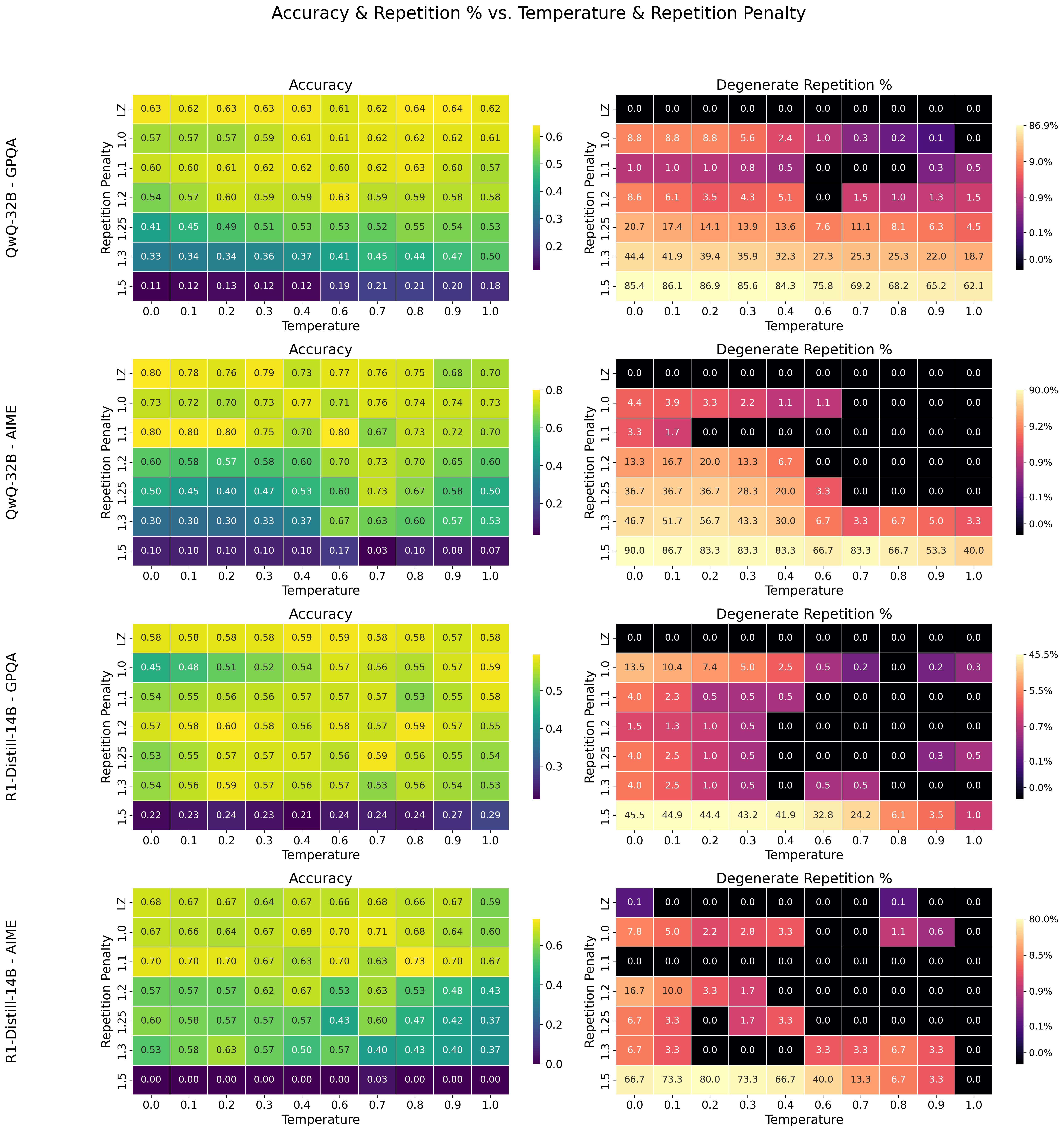
We apply the LZ penalty to QwQ-32B444Qwen/QwQ-32B and R1-Distill-14B555deepseek-ai/DeepSeek-R1-Distill-Qwen-14B. We run GPQA and AIME benchmarks (averaging scores and computing std. dev. over 5 runs). We set a max token limit of . We fixed the top-p to and the top-k to for all runs.666These are the recommended sampling parameters by the Qwen team For all runs also using the LZ penalty, we fix the penalty strength to , the window size to and the buffer size to . We found that this configuration of hyperparameters seemed to work well across both models and both datasets with minimal tuning required.777We only tested other penalty strengths in an original sweep of 0.1, 0.2, and 0.3. We found that 0.2 was sometimes too high and 0.1 was sometimes too low. Thus 0.15 seemed to be a sweet spot. The window and buffer sizes were selected on intuition and did not seem to require changing. We detect degenerate repetitions via dual verification of a GPT-4o based judge and a naive search for exact repetitions.888Any substring repeated at least 20 times.
Baselines
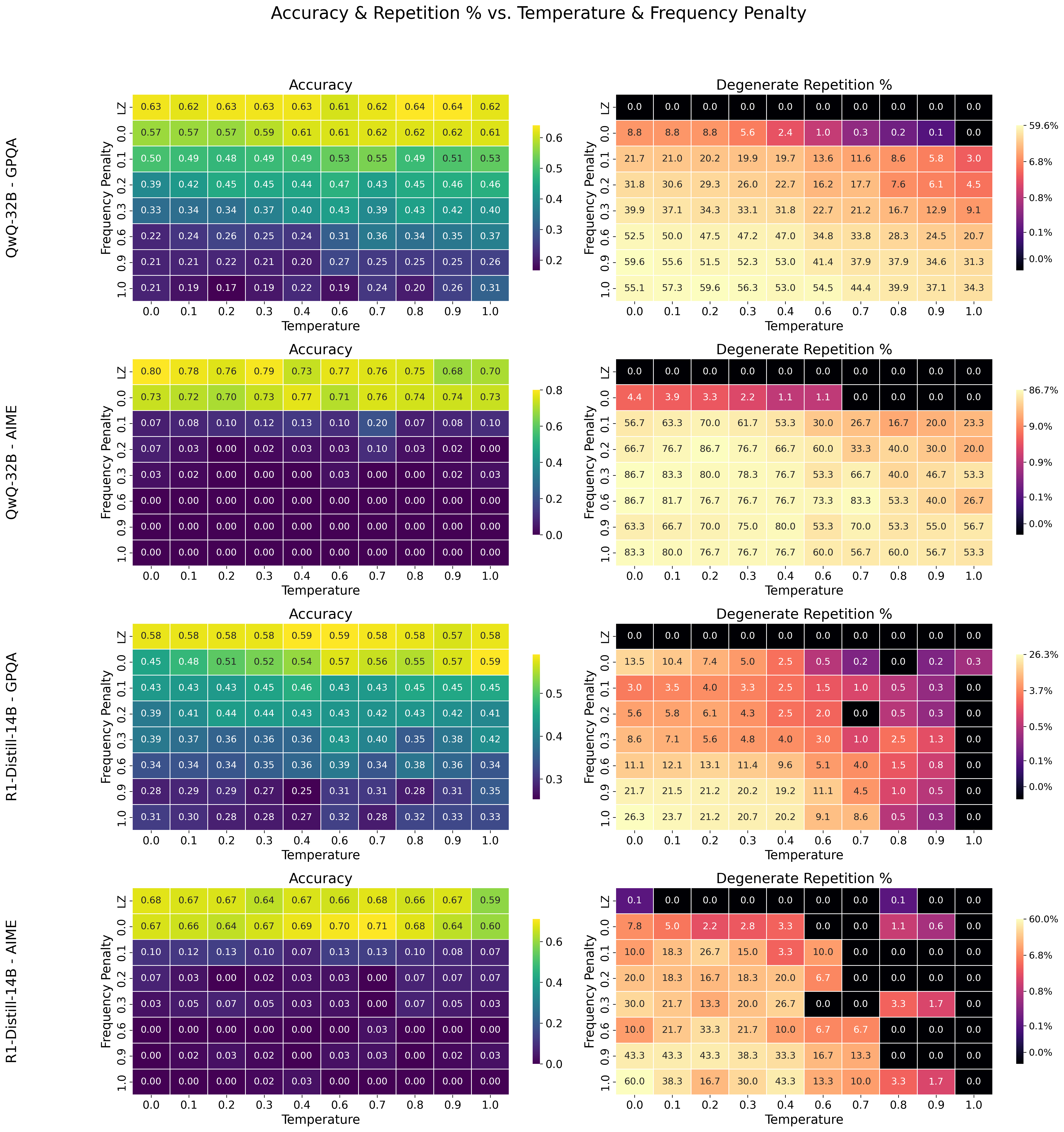
We compare the LZ penalty against two industry-standard penalties: the repetition penalty and the frequency penalty. In both cases, we finely sweep small values up until getting to large values. For the repetition penalty, we sweep with being the default value for a no-penalty baseline and being a standard value suggest by Keskar et al. (2019). For the frequency penalty, we sweep with being the default value for a no-penalty baseline.
Discussion
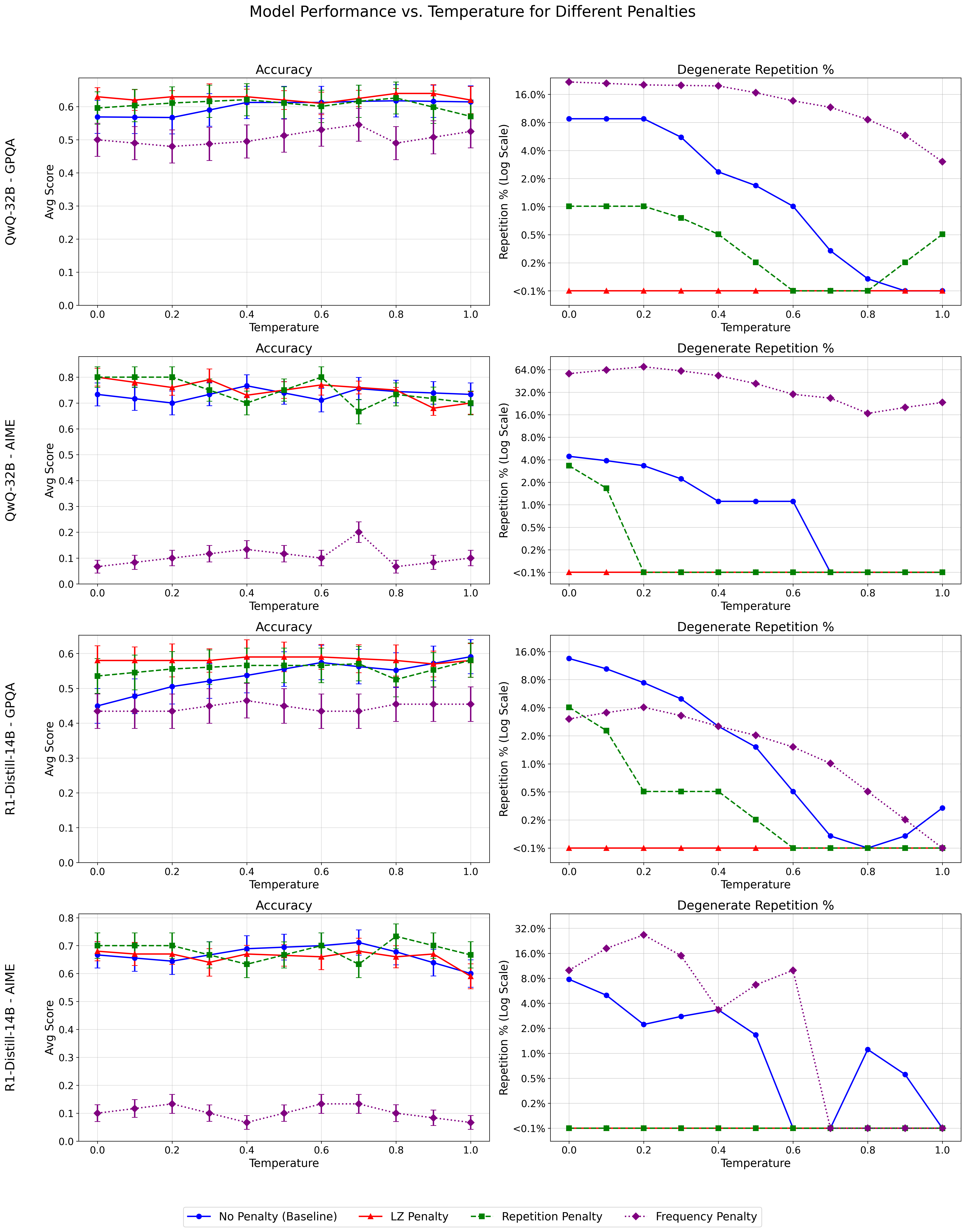
Based on Fig. 2 and Fig. 3, we observe that neither penalty is a reliable solution. The frequency penalty fails dramatically even for low values such as . We suspect that this is because of the length of the generations. Reasoning models produce reasoning traces that can be several thousand tokens long, which simply overwhelms the frequency penalty on common but essential tokens. This often results in a degradation that eventually collapses into a degenerate cycle behavior. The repetition penalty works significantly better than the frequency penalty and does seem to provide some modest relief at low temperatures. However, it is far from a complete solution, with low temperature degenerate repetition rates up to about depending on model and task domain. This would be disqualifying for any kind of serious application. On the other hand, the LZ penalty achieves effectively zero degenerate repetitions without affecting top-line benchmark scores. The LZ penalty works because it adaptively penalizes based on both the length of the match as well as how far back the match occurs. LZ penalty’s strength increases quickly in match length and attenuates gradually with distance. Both the repetition penalty and the frequency penalty operate at the single-token level whereas the LZ penalty operates at the -gram level. Furthermore, neither the repetition penalty nor the frequency penalty can forget tokens, whereas the LZ penalty quickly and then gradually weakens as the token becomes less recent, until it moves beyond the lookback window altogether and is ignored.
4.2 Latency and Throughput Benchmark
While our SGLang reference implementation is most certainly not fully optimized, we take minimum care to ensure that it is vectorized (and batched, assuming that the buffer size and lookback size are constant across the batch).999They should be. While we encourage exploration of these hyperparameters, we found buffer size of and lookback size of work well with minimal tuning.
We run SGLang’s built-in benchmark script on an H100 node and compare the effect of adding non-zero LZ penalty. While the LZ penalty adds an ultimately negligible amount of computation, it still is significantly more than, say, the repetition penalty, so this it is worthwhile to confirm that we can maintain inference performance.
We see that for larger models, the LZ penalty’s overhead is increasingly negligble. Even for models as small as B, the penalty overhead is a tolerable % throughput slowdown. For latency, the overhead is more trivial, and is not even measurable at the B size.
| Model Size | Med. Latency (ms) | Med. Throughput (tok/s) | Slowdown (%) |
|---|---|---|---|
| 1.5B | 4.43 | 14449.88 | – |
| 1.5B + LZ | 4.45 | 14370.98 | 0.55 |
| 7B | 7.96 | 4020.06 | – |
| 7B + LZ | 7.97 | 4014.29 | 0.14 |
| 32B | 26.71 | 299.55 | – |
| 32B + LZ | 26.71 | 299.47 | 0.03 |
References
- Keskar et al. [2019] Nitish Shirish Keskar, Bryan McCann, Lav R. Varshney, Caiming Xiong, and Richard Socher. Ctrl: A conditional transformer language model for controllable generation. arXiv preprint arXiv:1909.05858, 2019.
- Lempel and Ziv [1977] Abraham Lempel and Jacob Ziv. A universal algorithm for sequential data compression. IEEE Transactions on Information Theory, 23(3):337–343, 1977.
- Storer and Szymanski [1982] James A. Storer and Thomas G. Szymanski. Data compression via textual substitution. Journal of the ACM, 29(4):928–951, 1982.
- Shannon [1948] Claude E. Shannon. A mathematical theory of communication. Bell System Technical Journal, 27(3):379–423, July 1948. doi: 10.1002/j.1538-7305.1948.tb01338.x.
- Vaswani et al. [2017] Ashish Vaswani, Noam Shazeer, Niki Parmar, Jakob Uszkoreit, Llion Jones, Aidan N. Gomez, Łukasz Kaiser, and Illia Polosukhin. Attention is all you need. In Advances in Neural Information Processing Systems, pages 5998–6008, 2017.
- Jozefowicz et al. [2016] Rafal Jozefowicz, Oriol Vinyals, Mike Schuster, Noam Shazeer, and Yonghui Wu. Exploring the limits of language modeling. arXiv preprint arXiv:1602.02410, 2016.
- Welleck et al. [2019] Sean Welleck, Ilia Kulikov, Stephen Roller, Emily Dinan, Kyunghyun Cho, and Jason Weston. Neural text generation with unlikelihood training, 2019. URL https://arxiv.org/abs/1908.04319.
- Bowman et al. [2016] Samuel R. Bowman, Luke Vilnis, Oriol Vinyals, Andrew M. Dai, Rafal Jozefowicz, and Samy Bengio. Generating sentences from a continuous space. In Proceedings of the 20th SIGNLL Conference on Computational Natural Language Learning, pages 10–21, 2016.
- Holtzman et al. [2020] Ari Holtzman, Jan Buys, Li Du, Maxwell Forbes, and Yejin Choi. The curious case of neural text degeneration. In International Conference on Learning Representations, 2020.
- Radford et al. [2019] Alec Radford, Jeffrey Wu, Rewon Child, David Luan, Dario Amodei, and Ilya Sutskever. Language models are unsupervised multitask learners. OpenAI Blog, 2019. Technical report.
- Thoppilan et al. [2022] Romal Thoppilan, Daniel De Freitas, Jamie Hall, Noam Shazeer, Apoorv Kulikov, Ameet Prasad, Sharan Narang, et al. Lamda: Language models for dialog applications. arXiv preprint arXiv:2201.08239, 2022.
- Lempel and Ziv [1978] Abraham Lempel and Jacob Ziv. Compression of individual sequences via variable-rate coding. IEEE Transactions on Information Theory, 24(5):530–536, 1978.
- Wyner and Ziv [1994] A.D. Wyner and J. Ziv. The sliding-window lempel-ziv algorithm is asymptotically optimal. Proceedings of the IEEE, 82(6):872–877, 1994. doi: 10.1109/5.286191.
- Morita and Kobayashi [1993] H. Morita and K. Kobayashi. On asymptotic optimality of a sliding window variation of lempel-ziv codes. IEEE Transactions on Information Theory, 39(6):1840–1846, 1993. doi: 10.1109/18.265494.
- Fiala and Greene [1989] Edward R. Fiala and Daniel H. Greene. Data compression with finite windows. Communications of the ACM, 32(4):490–505, 1989.
- Miller and Wegman [1985] Victor S. Miller and Mark N. Wegman. Variations on a theme by ziv and lempel. Combinatorial Algorithms on Words, pages 131–140, 1985. NATO ASI Series, Volume F12.
- Pavlov [2007] Igor Pavlov. Lzma sdk (software development kit). Available at https://www.7-zip.org/sdk.html, 2007. Accessed: March 26, 2025.
- Oberhumer [1997] Markus F. X. J. Oberhumer. Lzo: A real-time data compression library. Available at https://www.oberhumer.com/opensource/lzo/, 1997. First released in 1997, Accessed: March 26, 2025.
- Yoshizaki [1988] Haruyasu Yoshizaki. Lha: A data compression and archiving tool. Software implementation, no formal publication, 1988. First released in 1988, combines LZSS with Huffman coding.
- Welch [1984] Terry Welch. A technique for high-performance data compression. Computer, 17(6):8–19, 1984.
- Cover and Thomas [2006] Thomas M. Cover and Joy A. Thomas. Elements of Information Theory. Wiley-Interscience, Hoboken, NJ, 2 edition, 2006.
- Paszke et al. [2019] Adam Paszke, Sam Gross, Francisco Massa, Adam Lerer, James Bradbury, Gregory Chanan, Trevor Killeen, Zeming Lin, Natalia Gimelshein, Luca Antiga, Alban Desmaison, Andreas Kopf, Edward Yang, Zachary DeVito, Martin Raison, Alykhan Tejani, Sasank Chilamkurthy, Benoit Steiner, Lu Fang, Junjie Bai, and Soumith Chintala. PyTorch: An imperative style, high-performance deep learning library, 2019. URL https://pytorch.org/.
- Witten et al. [1987] Ian H. Witten, Radford M. Neal, and John G. Cleary. Arithmetic coding for data compression. Communications of the ACM, 30(6):520–540, 1987.
- Huffman [1952] David A. Huffman. A method for the construction of minimum-redundancy codes. Proceedings of the IRE, 40(9):1098–1101, 1952.
- Ryabko [2007] Boris Ryabko. Compression-based methods for nonparametric density estimation, on-line prediction, regression and classification for time series, 2007. URL https://arxiv.org/abs/cs/0701036.