Benchmarking field-level cosmological inference from galaxy redshift surveys
Abstract
Field-level inference has emerged as a promising framework to fully harness the cosmological information encoded in next-generation galaxy surveys. It involves performing Bayesian inference to jointly estimate the cosmological parameters and the initial conditions of the cosmic field, directly from the observed galaxy density field. Yet, the scalability and efficiency of sampling algorithms for field-level inference of large-scale surveys remain unclear. To address this, we introduce a standardized benchmark using a fast and differentiable simulator for the galaxy density field based on JaxPM. We evaluate a range of sampling methods, including standard Hamiltonian Monte Carlo (HMC), No-U-Turn Sampler (NUTS) without and within a Gibbs scheme, and both adjusted and unadjusted microcanonical samplers (MAMS and MCLMC). These methods are compared based on their efficiency, in particular the number of model evaluations required per effective posterior sample. Our findings emphasize the importance of carefully preconditioning latent variables and demonstrate the significant advantage of (unadjusted) MCLMC for scaling to -dimensional problems. We find that MCLMC outperforms adjusted samplers by over an order-of-magnitude, with a mild scaling with the dimension of our inference problem. This benchmark, along with the associated publicly available code, is intended to serve as a basis for the evaluation of future field-level sampling strategies. The code is readily open-sourced at github.com/hsimonfroy/benchmark-field-level.
1 Introduction
In the current cosmological model the evolution of the Universe is governed by a small set of cosmological parameters. Inflation gives rise to an initial field of primordial fluctuations, which evolve under gravity to form the large scale structure (LSS) of the Universe. Galaxy surveys such as DESI [1], Euclid [2], and Vera Rubin’s Legacy Survey of Space and Time [3] serve as powerful probes of LSS by mapping the spatial distribution of galaxies, which traces the underlying matter density field and provides a direct observational signature of the evolved primordial fluctuations.
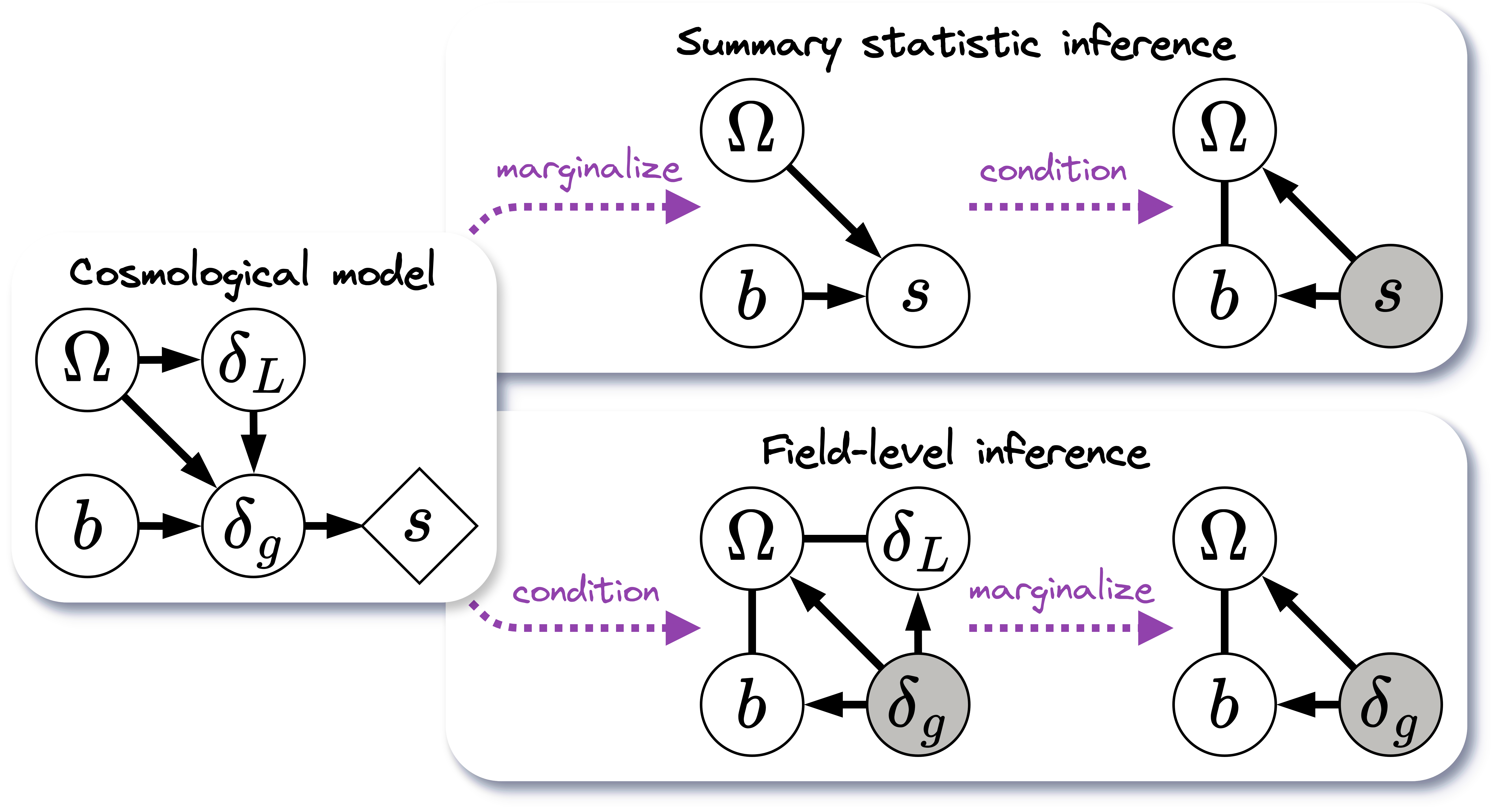
A common approach to extracting information from galaxy surveys is to compress the observed galaxy density field into a summary statistics . As illustrated in figure 1 (top panel), a marginal likelihood , is then constructed to relate cosmological parameters and a reduced set of nuisance parameters to the summary statistics , effectively marginalizing over the stochasticity of the fields and . This marginalization can be performed with a Gaussian model, e.g. with analytical or simulation-based mean and covariance [4], or with more general techniques of Neural Density Estimation, e.g. normalizing flows, also fitted on simulations [5]. Finally, the posterior distribution is inferred, often using Markov Chain Monte Carlo (MCMC) sampling. The choice of summary statistics is guided by a trade-off between analytical or variational tractability of its likelihood, and the amount of cosmological information retained.
A well-motivated choice for is the power spectrum of . On large scales, where the field remains approximately Gaussian, the power spectrum is close to being sufficient statistics, i.e. . Additionally, the power spectrum likelihood is relatively tractable, as it can often be well approximated by a Gaussian distribution with an analytical mean. Yet, gravity-driven structure formation is non-linear, making the galaxy density field non-Gaussian. In this case, the power spectrum is not sufficient, hence the development of analyses relying on alternative statistics [6], such as higher order statistics (3PCF [7], bispectrum [8]), object correlations (peaks [9], voids [10, 11], density splits [12, 13],…), multiscale counts (wavelet scattering transform [14], 1D-PDFs [15], Minkowski functionals [16, 17], k-nearest neighbors [18], Betti numbers [19]…), or automatically-learned statistics (CNN compression [5] or GNN compression [20]). Nonetheless, striking a balance between the interpretability of the compressed statistic, the tractability of its likelihood, and its ability to probe the cosmological signal exhaustively, remains a fundamental challenge.
An alternative approach, known as field-level inference, bypasses the need for summary statistics by directly conditioning on the observation . It proceeds so by jointly sampling the initial linear field with cosmology and nuisance parameters , as illustrated in figure 1 (bottom panel). The marginal posterior is then readily obtained by discarding samples. These samples also enable a posterior reconstruction of the Universe’s history at the field level, as illustrated by figure 2 or by [21]. By construction, this approach extracts all the information encoded in the (observed and discretized) galaxy density field and is therefore quasi lossless. However, applying it to the volume of a large-scale survey like DESI (), discretized at a typical non-linear scale of \qty5\mega/, results in inferring a latent field with parameters. Field-level inference thus shifts the challenge from performing analytical or variational marginalization to solving a high-dimensional sampling problem.

To tackle this, state-of-the-art sampling methods, such as the Hamiltonian Monte Carlo (HMC) algorithm [22, 23], leverage the gradient information to efficiently explore high-dimensional posteriors. In practice, the requirement for the gradient is a mild constraint on the model implementation, as modern computational frameworks like JAX111github.com/jax-ml/jax [24] enable automatic differentiation, eliminating the need for manual derivations. HMC is used in most field-level inference applications [25, 21, 26, 27, 28, 29, 30]. The No U-Turn Sampler (NUTS) [31], a variation of the standard HMC algorithm with automatically tuned trajectory length, has been used by [32, 33]. [34] recently proposed a different sampler dubbed MicroCanonical Langevin Monte Carlo (MCLMC) to perform cosmological field-level inference, showing it can require over an order-of-magnitude less model evaluations than HMC. Moreover, the choice of reparametrization, i.e. model preconditioning strategies, generally affects the efficiency of these sampling methods. A comprehensive comparison of these strategies is required to identify the most efficient and robust approaches, to assess their scalability to next-generation galaxy surveys, and to guide future algorithmic developments.
In this work, we conduct a comprehensive benchmark of MCMC samplers and preconditionings, focusing on field-level modeling and inference for galaxy clustering data. Our goal is to identify strategies that enable reliable posterior sampling while minimizing the number of computationally expensive simulations. Additionally, we investigate how modeling choices, such as resolution, volume, and complexity in large-scale structure formation modeling impact the high-dimensional sampling process.
2 Methodology
2.1 Model
To benchmark various sampling strategies under the most relevant conditions, we implement a forward model that encapsulates the key physical processes that could impact high-dimensional field-level sampling. These include the initial matter field generation, its non-linear gravitational evolution, the galaxy-matter connection, redshift-space distortions (RSD), and observational noise. The analysis is performed in a self-specified context, where the observations are generated from the same model used for inference. This idealized setting allows us to isolate and study the performance of sampling algorithms without the confounding effects of model misspecification [35, 36]. Questions related to the convergence of the density and velocity fields at the probed scales, as well as survey-specific modeling choices (e.g. selection functions, observational systematics) are deferred to future work. By focusing on the fundamental components of galaxy clustering models while remaining agnostic to specific survey characteristics, this modeling is designed to be broadly informative for upcoming applications of field-level inference to galaxy surveys.
In practice, we make use of JAX, a Python library providing GPU acceleration, Just-In-Time (JIT) compilation, automatic vectorization/parallelization, and differentiation. We implement our model via NumPyro222github.com/pyro-ppl/numpyro [37], a Probabilistic Programming Language (PPL) powered by JAX, which facilitates model definition, differentiation, and sampling. Our hierarchical model is thus highly modular, and contains the following stages:
-
1.
Initial matter field: cosmological parameters include the matter density , and the amplitude of linear fluctuations (smoothed at a scale of ) . The linear matter field is then sampled as a Gaussian field, with power spectrum determined by these parameters via the fitting formula of [38] implemented in jax-cosmo333github.com/DifferentiableUniverseInitiative/jax_cosmo [39].
-
2.
LSS formation: matter particles are initialized on a regular grid and displaced following first/second order Lagrangian Perturbation Theory (1LPT/2LPT), or through a Particle Mesh (PM) N-body scheme. We rely on JaxPM444github.com/DifferentiableUniverseInitiative/JaxPM, which is a JAX version of FlowPM [40]. To compute N-body displacement in particular, we use 5 steps of the BullFrog solver, recently proposed by [41], and implemented within JaxPM framework. In addition to faster convergence, BullFrog does not require prior LPT initialization, eliminating the sensitivity to the starting redshift of other PM solvers, like FastPM [42].
-
3.
Redshift-Space Distortions: particles are advected once more according to their velocities projected along line-of-sight to account for contribution of galaxy peculiar velocity to redshift measurement. The RSD displacement depends on the Hubble function , evaluated at the simulation redshift , and is given by
(2.1) where line-of-sight is fixed and taken to be one axis of the grid.
- 4.
-
5.
Observational noise: the biased field is then converted into the observed galaxy density field , by adding Gaussian noise with variance to each voxel, where is the average number of galaxies per voxel.
In total, the latent parameters include 2 cosmological parameters ; 4 bias parameters from the second order Lagrangian bias expansion ; and the linear matter field , whose dimensionality depends on discretization of the simulated volume. These latent parameters are preconditioned to improve sampling efficiency, which means that the base variables are reparametrized into sample variables whose posteriors are closer to a standard Gaussian. We refer to section 2.3 for details on the different conditioning strategies. The true values of and used in experiments (to generate synthetic data), their priors, as well as the fiducial values taken to compute the initialization and the static preconditioning (see section 2.3) are referenced in table 1. The prior ranges for bias parameters are typical of values measured from N-body simulations populated with Halo Occupation Distribution scheme [45] and we ensure in the following that computed posteriors are likelihood-dominated.
| Name | Symbol | Truth | Prior | Fiducial |
|---|---|---|---|---|
| Matter density | 0.3 | 0.3111 | ||
| Amplitude of linear fluctuations | 0.8 | 0.8102 | ||
| Lagrangian galaxy bias | 1 | 1 | ||
| 0 | 0 | |||
| 0 | 0 | |||
| 0 | 0 |
As a baseline in this work, we simulate a cosmological volume of discretized into a mesh, resulting in a voxel resolution of \qty5\mega/. Also, is fixed assuming a DESI-like mean galaxy density of .
2.2 MCMC samplers
To perform the high-dimensional sampling required in field-level inference, we cannot afford to employ a classical Metropolis-Hastings (MH) algorithm. This algorithm samples a target density via a simple Markov chain where each step is agnostic to local information about the density. This leads to two major issues: (i) as the dimensionality increases, more directions lead away from high-density regions, so that the step size must scale as to maintain a given acceptance rate; (ii) once the dynamics has reached high-density regions, motion becomes locally Brownian (a random walk), meaning steps of size are required to move by , which is an inherently slow way to explore the sampling space.
Addressing these issues requires integrating local information about the target density into the dynamics. Moreover, significant advances in numerical sampling and optimization have been achieved by exploiting their connection to statistical physics: many randomized iterative methods exhibit particle-like dynamics, which can be analyzed statistically and leveraged to inform new developments. The following subsections provide an overview of canonical and microcanonical Langevin MCMC methods to introduce the different samplers that we consider in our benchmark.
2.2.1 Canonical sampling with Langevin dynamics
Our goal is to sample from the -variate target density . In the canonical potential evolves a particle of position , momentum , and mass (matrix) . The Hamiltonian of this particle is then given by:
| (2.3) |
As a result, its motion follows Hamilton equations
| (2.4) |
which constrain the particle to the constant-energy surface , where denotes the initial particle energy. Confined to this surface, the particle cannot sample from a general target density without energy exchange.
Energy exchange can be provided by the particle’s surrounding medium, a heat bath, where it collides with other particles at a frequency . The resulting dynamics in the continuous limit of interaction is described by the Langevin equations
| (2.5) |
where is a Wiener process (so is a Gaussian white noise). These equations add to the Hamiltonian dynamics a dissipation term and a fluctuation term , which account respectively for the particle dissipating coherent kinetic energy as heat and gaining dispersed kinetic energy from thermal fluctuations.
Energy exchange allows the particle system to reach thermal equilibrium, where the distribution of particle states is given by the canonical ensemble . In particular and as desired, the particle position is distributed as the target :
| (2.6) |
2.2.2 Microcanonical sampling with isokinetic Langevin dynamics
A limitation of introducing energy exchange into the dynamics is that the target distribution is only recovered by averaging particle trajectories across multiple energy levels, potentially slowing convergence. Hopefully, energy exchange is not necessary if, instead of a classical particle, we consider an isokinetic particle, i.e. a particle of constant kinetic energy , where denotes an auxiliary momentum.
Physically, this isokineticity can be enforced by coupling the particle to a Gaussian IsoKinetic (GIK) thermostat [46], which constantly extracts or provides energy to the particle so that its temperature, as a kinetic energy, is a constant of motion (see appendix A). When placed in the rescaled potential (recalling is dimension), such particle admits the GIK Hamiltonian555In contrast to [47, 48, 49] we adopt the GIK Hamiltonian formulation that does not require any momentum-dependent time rescaling. This preserves as a stationary density of the dynamics, and therefore reconciles the microcanonical formulation from [47, 48] and the isokinetic formulation from [49]. In appendix A, we show that we can rederive from this Hamiltonian the MCLMC equations of motion.
| (2.7) |
where and is the canonical momentum. Remarkably, this Hamiltonian’s microcanonical ensemble coincides exactly with its isokinetic ensemble . This means that under ergodicity, the particle is sampling these ensembles, and therefore has position distributed as target :
| (2.8) |
However, merely following the induced Hamiltonian dynamics does not ensure the ergodicity required for sampling the microcanonical/isokinetic ensemble. In fact, if the system exhibits additional symmetries beyond time translation (which already enforces energy conservation), Noether’s theorem guarantees the opposite: the particle remains confined to a subset of the constant-energy surface defined by an additional conserved quantity.
To ensure ergodicity, [48] reintroduces the particle into a heat bath, where it collides with other particles at a frequency . However, due to the GIK thermostat, these interactions always conserve kinetic energy. For numerical efficiency, it is preferred to compute the dynamics for state , rather than , which follows in the continuous limit of interaction the isokinetic Langevin equations [49] (in Stratonovich form)
| (2.9) |
where is the orthogonal projection onto . Therefore thermal fluctuations only impact the momentum direction while both Hamiltonian and kinetic energy are conserved.
2.2.3 Derived samplers
The Langevin dynamics modeled by equations 2.5 and 2.9 are the basis of several sampling algorithms, involving different regimes of interaction with medium and inertia . In practice, the dynamics are solved numerically, often using symplectic integrators like KDK-Verlet/Leapfrog or McLachlan/Minimum-Norm integrator [50]. Numerical integration comes with discretization errors that can induce a bias, which can be either eliminated via MH adjustement (accept-reject step), or controlled via the integration step size.
In this benchmark, we consider three canonical and adjusted samplers, and two microcanonical samplers. Our selection is guided by both the existing literature on field-level inference and the availability of the implementations. It is designed to highlight key methodological distinctions, particularly between canonical vs. microcanonical, and adjusted vs. unadjusted methods.
HMC.
The celebrated Hamiltonian Monte Carlo algorithm [23] simulates a classical particle evolving according to equations 2.5 in a sparse medium () for a tunable trajectory time length , before colliding with a heavy particle, which refreshes its momentum: . This arrival state is then used as a proposal for a MH adjustement step, after which the dynamics repeats.
NUTS.
No-U-Turn Sampler [31] is a variant of HMC that automatically and dynamically adapts the trajectory time length . It constructs sets of proposals along the Hamiltonian trajectories, which are stopped whenever they start to reverse direction, thereby avoiding redundant exploration and the need for manual tuning of .
NUTSwG.
Any MCMC sampler can be implemented within a Gibbs sampling scheme [51], where MCMC sampling alternates over subsets of parameters. For instance, assume one wants to sample from three blocks of variables . Then a MCMC within Gibbs scheme consists in sampling alternatively with the given MCMC from , then , then , using the sample of one block to condition the others. It can be seen as a sampling generalization of alternating gradient descent. We consider a NUTS within Gibbs implementation, referred to as NUTSwG in the following.
MAMS.
Metropolis-Adjusted Microcanonical Sampler [52] is a microcanonical counterpart to canonical HMC. It simulates an isokinetic particle evolving according to equations 2.9 in a sparse medium () for a tunable average trajectory time length , before colliding with a heavy particle, which refreshes its momentum: where . This arrival state is then used as a proposal for a MH adjustement step, after which the dynamics repeats.
MCLMC.
MicroCanonical Langevin Monte Carlo [48] simulates an isokinetic particle evolving according to equations 2.9 in a dense medium. There, the particle undergoes continuous collisions with lightweight particles, causing its momentum to be partially refreshed at each integration step: , where ,666This refreshment step replaces the less direct-to-sample Brownian motion on the hypersphere [53], corresponding to the diffusion term in equations 2.9. Both preserve as a stationary density and provide the desired ergodicity [49], and they even closely agree when . and the tunable momentum decoherence length is introduced such that . Crucially, MCLMC is run without MH adjustement step, meaning that every integration state is directly accepted as a sample. Any potential bias introduced by this unadjusted scheme is controlled by the integration step size , as discussed below.
On the one hand, adjusted algorithms are asymptotically unbiased, but at the cost of significantly reducing the integration step size as dimension increases in order to maintain a reasonable acceptance rate. Formally, [23] show that for a target product density, the number of model evaluations needed to reach a new effective sample grows as for the MH algorithm, as for adjusted overdamped () Langevin dynamics, and as for adjusted underdamped () Langevin dynamics.
On the other hand, unadjusted algorithms have no unbiased guarantees, but the relation between step size and bias has been theoretically studied for both canonical and microcanonical samplers [54, 55]. In particular, [55] show, both formally for a target isotropic Gaussian and empirically, that the bias can be controlled via , the Energy Error Variance Per Dimension (EEVPD) across integration steps, which itself depends on the step size in a dimension-independent manner. Therefore, by tuning the step size to keep the EEVPD below some threshold, one ensures that the total sampling error (in terms of Wasserstein distance or Mean Square Error) is dominated by the Monte Carlo error. Effectively, this EEVPD threshold governs the trade-off between the sampling efficiency (the number of model evaluations needed to reach a new effective sample) and the bias, independently of the dimension. This is a really promising result compared to the scaling of adjusted methods. Admittedly, the sampled posterior is rarely an isotropic Gaussian in practice, so we may expect some dependency of the sampling efficiency to dimension. However, as explained in section 2.3, we can reparameterize the model such that the posterior approaches an isotropic Gaussian.
2.3 Conditioning strategies
For any sampling problem, one is free to choose any bijective reparametrization of the base variables. Formally, sampling from a target density in a variable space is analytically equivalent to sampling from the image density in the transformed space , and then transforming back the samples to . However, these are not algorithmically equivalent. The density in can be challenging to sample (due to degeneracies, discontinuities, boundaries, etc.), but a transformed space can often be defined where the density is smoother and easier to sample. This section focuses on preconditioning the latent space so that the posterior of latent variables approximates an isotropic Gaussian.
2.3.1 Model preconditioning
With full knowledge of the posterior, finding a suitable reparameterization would be simplified. But in practice, when sampling is precisely the way we access posterior information, we can only rely on partial posterior knowledge. A simple preconditioning is prior-conditioning, where (a priori) sample variables are made isotropic Gaussian. This is a relevant choice of conditioning if the likelihood constraining power is weak or aligned with the prior, as the resulting prior-conditioned posterior would also be approximately isotropic Gaussian. However, if the likelihood constraining power is strong and varies significantly across variables relatively to their priors, prior-conditioning can exacerbate degeneracies in the posterior [56].
In the context of field-level inference, model preconditioning is exemplified by the choice of parametrization for the linear field . The linear field can easily be prior-conditioned in real space by considering a Gaussian white noise, which is Fourier-transformed and multiplied by the square root of the power spectrum. However, the likelihood typically induces correlations between voxels, leading to a posterior that is ill-conditioned. Alternatively, the linear field can also easily be prior-conditioned in Fourier space with a complex Hermitian Gaussian noise, multiplied by the square root of the power spectrum. As a result of the large-scale isometry-invariance and linear growth of , the posterior wavevector amplitudes are approximately independent and Gaussian. However, since different scales are constrained with varying power, the posterior can still remain poorly conditioned.
In order to make the posterior more isotropic, we approximate it assuming a linear model for the observed galaxy density field, as described hereafter. In Fourier space, for any wavevector , the linear matter field is distributed as a complex-Gaussian , recalling that for any complex vector and covariance matrix . In the flat-sky approximation, this field is then evolved linearly by a factor known as the Kaiser boost [57], where and are the linear growth factor and growth rate at the observed redshift and cosmology, is the linear Eulerian bias associated to the linear Lagrangian bias , and is the cosine of the angle between wavevector and line-of-sight . Finally, as in the reference forward model, we include observational noise as a Gaussian distribution of variance , the mean number of galaxies per voxel. Put together and applying Bayes formula for this Gaussian linear model, we have
| (2.10) |
with
meaning that we a posteriori have . Hence we define the preconditioned linear field:
| (2.11) |
such that its estimated posterior is as desired . This reparametrization obviously depends on cosmology and bias parameters, which we specify following these two options (that we compare in section 3.3):
-
1.
Static Kaiser conditioning: we assume fixed fiducial values , as given in table 1.
-
2.
Dynamic Kaiser conditioning: we use the values of of the current sample, thereby adapting the conditioning to the local shape of the posterior.777This is equivalent to an analytical and spatially-varying Riemannian metric, as leveraged in Riemannian Manifold Hamiltonian Monte Carlo (RMHMC) [58].
Cosmological and bias parameters are also transformed into based on a rough estimate of their posterior standard deviation , such that is approximately a standard Gaussian. To estimate , we observe that it scales as the inverse square root of the galaxy sample volume and extrapolate the constraints from a fast (low-dimensional) inference performed within a smaller volume.
The preconditioning strategy described above leverages approximate knowledge of the posterior to enhance sampling efficiency. However, at smaller scales, the Kaiser model approximation no longer holds888In addition, when considering observational data, the spatially-varying survey selection function will introduce correlations between wavevectors.. To further improve the model conditioning, we can rely on an adaptive mass matrix.
2.3.2 Mass matrix conditioning
The MCMC samplers we introduced in section 2.2 all admit a mass matrix as a tunable parameter. Formally, a particle of position and mass will follow the same dynamics (up to a time and initial momentum rescaling) as a particle of position and unit mass , i.e. the mass matrix is equivalent to a linear conditioning of the sample positions. Therefore, a good candidate for the mass matrix is the inverse covariance of the sample variables [59].
The adopted strategy is to leverage prior knowledge to analytically precondition into as described in section 2.3.1, then rely on adaptive methods to set , where is an online estimate of the covariance of . In practice, this estimation is performed during a warmup phase using Welford’s algorithm for numerical stability, and the mass matrix is kept diagonal for computational efficiency.
2.4 Metrics
The performance of an estimation procedure can be quantified via its associated risk , such as the Mean Square Error (MSE). For a given number of data samples, the efficiency compares the risk of a particular estimator to the risk of a reference estimator . Alternatively, the number of samples needed for the reference risk to equate the particular risk, , is commonly referred to as the Effective Sample Size (ESS).
In our case, we obtain from MCMC sampling a stationary and identically distributed, but possibly correlated, sequence of samples, from which we are interested to estimate some target quantity (e.g. mean, median, covariance, quantile, credible region…). We can then compare the MSE based on the correlated sequence with the MSE that we would have if the samples were independent. The induced ESS denoted is then understood as “the number of independent samples that would yield the same statistical power as the MCMC samples for estimating the quantity ”. Typically, it is the sample size at which the (Markov Chain) Central Limit Theorem operates for this quantity, i.e. .
It is common and simpler to focus on the estimation of the mean , so in the following, the ESS denoted by refers to unless otherwise specified. Formally, for a stationary sequence of size and autocorrelation , the ESS is asymptotically
| (2.12) |
and can be estimated based on sample autocorrelation. We see that in the stationary case, the more correlated the samples are, the smaller the ESS becomes. This aligns with the common (though not always true) intuition that highly correlated samples share redundant information, thus reducing their overall effectiveness.
The ESS is a relevant metric for quantifying the quality of a sample sequence, serving as a proxy for estimation error without requiring knowledge of the true mean value. On the other hand, if their true value is known, we can directly compute the error for any quantity of interest, typically the mean and standard deviation . Given chains, we estimate their mean and standard deviation , and the (empirical and normalized) MSE is obtained as:
| (2.13) |
Normalization of errors ensures that for an asymptotically unbiased estimator , making it commensurable with the inverse ESS.
Given the high dimensionality of our problem, it is often necessary to aggregate metrics across sets of variables, such as cosmological, bias, and linear field parameters. The multivariate generalization of MSE implies that we respectively take the arithmetic mean of empirical MSEs and the harmonic mean of ESSs.
Model evaluation (especially its gradient) is our main computational bottleneck for cosmological inference. We therefore characterize the efficiency of a MCMC sampler by the number of model evaluations required to yield one effective sample , and commensurably, to yield a unit error . These metrics are expected to be relatively stable over evaluations, so we check their convergence before reporting them.
Finally, unadjusted samplers may introduce an asymptotic bias in the sampled posterior (see appendix B), that is not directly quantified by the ESS or the MSE individually999A high MSE can be caused by both an inefficient sampling (low ESS) or a bias.. However, since in the unbiased case, is of the order of the inverse ESS, finding would reveal a non-negligible bias.
3 Numerical Results
In this section we benchmark a comprehensive range of sampling methods and conditioning strategies according to the metrics specified in section 2.4 for the model presented in section 2.1. The task is to sample from the posterior given an observation generated from the same model. In sections 3.2 and 3.3, the forward model performs 1LPT displacement in a volume discretized into a mesh (voxel resolution of ). In section 3.4, we vary these settings.
We run for each inference task 8 parallel chains, on GB NVIDIA A100 GPU node. Our sampling pipeline is built upon JAX-powered packages NumPyro and BlackJAX101010blackjax-devs.github.io/blackjax [60].
3.1 Initialization
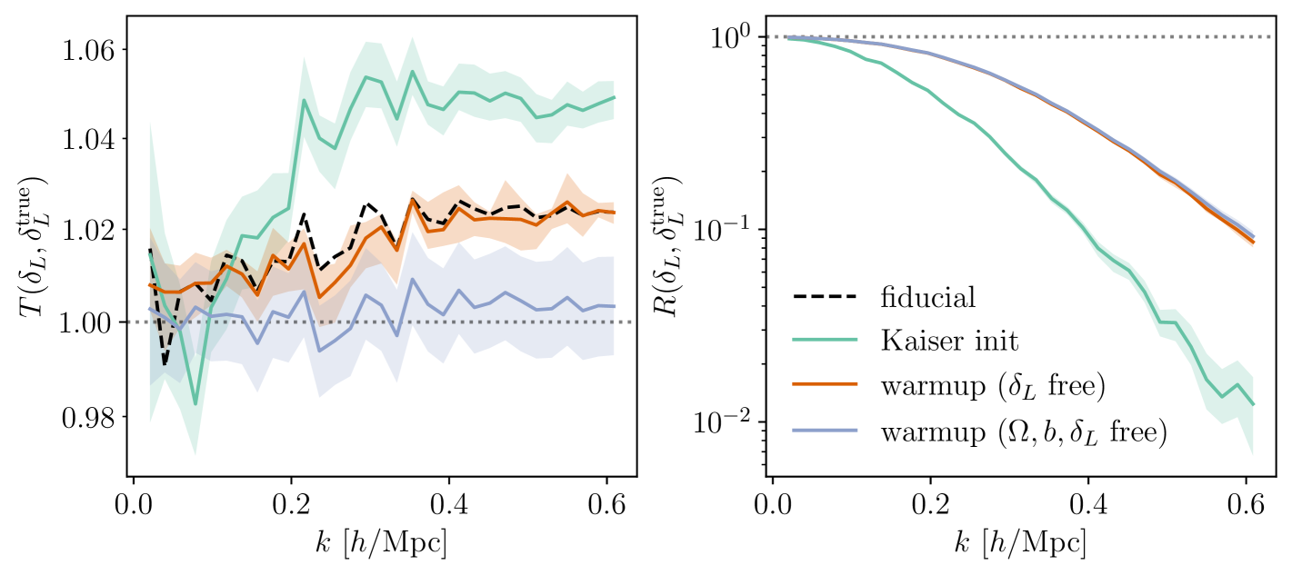
Simply drawing samples from the prior would produce an initial field with the fiducial power spectrum, but its amplitudes and phases would be distributed between the different wavevectors regardless of the observed field . Instead, we seed the chains with samples from the Kaiser posterior, given by equations 2.10 and fiducial parameters. This approximation results in an inaccurate initial linear power spectrum but aligns amplitudes and phases closer to their high-density regions. This is especially the case for the largest scales as reflected by the spectra correlation111111Because spectra correlation is complex-valued, we only show its norm, though we may miss some potential phase shifts. on figure 3. We observe that this initialization strategy indeed accelerates convergence.
We then perform a first warmup phase where exclusively is inferred while maintaining other (cosmological and bias) parameters fixed at their fiducial values. This allows the high-dimensional to converge towards its high-density region while preventing its dynamics to drag the other parameters away. This warmup phase is assumed successful when the sample power spectrum fluctuates around the fiducial one, as shown by the transfer function on figure 3. Note that if we had initialized the linear field from the start with the fiducial power spectrum, we would not be able to rapidly distinguish the chain convergence from the chain being stuck.
Next, a second warmup phase is performed where all parameters are jointly sampled. This is also the phase where sampler hyperparameters are tuned, especially step size and mass matrix. This second warmup is assumed successful when the sampler hyperparameters of the different chains are in qualitative agreement.
Finally, the chains are run until reaching at least 500 ESS and a Gelman-Rubin statistic of at most for each parameter (which is roughly equivalent, see [61]).
In total, about one fifth of the total number model evaluations is spent for warmup (to be conservative), and we do not include these evaluations in the benchmark results. We observe that a short warmup time is, as expected, correlated with a high sampling efficiency in the stationary regime.
3.2 MCMC samplers
We start by comparing the performance of the different samplers mentioned in section 2.2. For all samplers, we use the Kaiser dynamic preconditioning and tune a (diagonal) mass matrix. Their specific configurations are described hereafter:
HMC, NUTS, NUTSwG.
We solve the equations of motion 2.4 with the KDK-Verlet integrator and tune the step size to obtain a acceptance rate, theoretically optimal for product densities [23], which we corroborated in our tests.121212The relevant range of the target acceptance rate for HMC-like algorithms is usually , with higher values better suited to more complex densities [31, 62].
HMC.
The trajectory time length is based on the average trajectory length of NUTS, following the heuristic .131313Hamiltonian trajectory length is fixed here, although randomizing it could improve certain performance metrics in some cases [63].
NUTSwG.
We split the sampled variables into two blocks: (i) the linear field and (ii) cosmological and bias parameters , in a similar fashion to [26, 29]141414This choice can be partly motivated by a lack of differentiable computation of cosmological quantities. In the referenced works, each cosmological and bias parameter is itself treated in a separate block.. A NUTS within Gibbs scheme for these blocks means that we alternatively sample with NUTS from then , using the sample of one block to condition the others. We also tested splitting the parameter space between and , based on the idea that sampling is computationally cheap since it only involves evaluating the bias model and does not require simulating structure formation. However, even under the optimistic counting of zero model evaluation for a recomputation of the bias model, this approach performed worse than the other sampling methods.
MAMS, MCLMC.
We tested a variety of symplectic integrators151515The specific interest of symplectic integrators for solving equations 2.9 is not direct since it is not formulated in canonical phase space . to solve the equations of motion 2.9. This includes the widely used KDK-Verlet integrator (2nd-order, 1 model evaluation per step), McLachlan integrator (2nd-order, 2 evaluations; see eq. 4.2 in [50]), Blanes integrator (2nd-order, 3 evaluations; see eq. 44 in [64]), and Omelyan integrator (4th-order, 5 evaluations; see eq. 77 in [65]). The McLachlan and Omelyan schemes are known to achieve minimum norm within their respective orders [66], while the Blanes scheme offers best stability among 3-evaluation methods. In our tests, the McLachlan integrator consistently achieved the best performance, albeit by a modest margin, and is therefore adopted in the remainder of this work. As expected, more stable or higher-order integrators allowed for larger step sizes, but the gain was insufficient to offset their increased number of model evaluations.
MAMS.
The step size is tuned to obtain a acceptance rate, theoretically optimal for product densities and corroborated in our tests.161616[52] report higher values working well in their tests, which may be better suited for more complex densities. The average trajectory length is set to heuristic (with for McLachlan integrator) [52], where is a rough estimate of the (multivariate) ESS.
MCLMC.
The step size is tuned to obtain an EEVPD below , ensuring negligible bias in the posterior distribution. A detailed discussion on this choice, along with the potential bias of MCLMC. A detailed discussion on the followed strategy to control the potential bias of MCLMC is provided in appendix B. We set the momentum decoherence length according to a worst-case heuristic , where is a rough estimate of the ESS of the -th sampled variable. Contrary to adjusted samplers that yield one sample after a certain number of integration steps , MCLMC yields one sample at each step. However, saving all these correlated samples is memory inefficient, so we apply chain thinning, retaining only every 16th step. We verify that this does not impact the performance metrics.
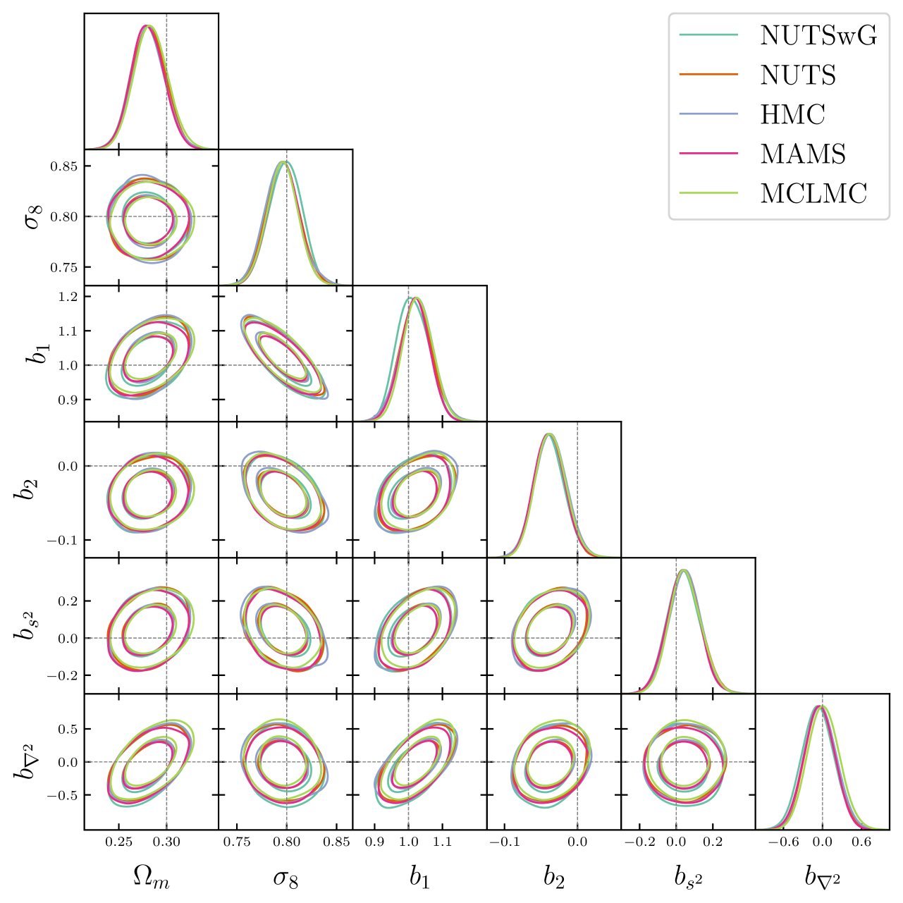
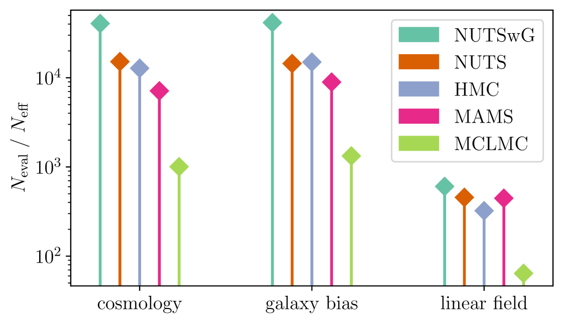
The posterior obtained for different samplers are in good agreement, as illustrated in figure 4. Moreover, figure 5 shows the number of model evaluations per effective sample for each sampler and each set of parameters. Both microcanonical samplers, MAMS and MCLMC, outperform their canonical counterparts. Notably, MCLMC surpasses all adjusted samplers, achieving a tenfold speedup in this case. In particular, when compared to MAMS, this suggests that for such high-dimensional settings, the efficiency gain stems primarily from the unadjusted nature of MCLMC, with its microcanonical nature playing a secondary role.
Also, NUTSwG performs worse than standard NUTS, which is expected since MCMC within Gibbs sampling is theoretically suboptimal, particularly for correlated densities. While preconditioning and mass matrix tuning help mitigate correlations (see section 3.3), residual correlations may still contribute to this performance gap. Finally, HMC performs slightly better than NUTS, but this comparison benefits from the fact that HMC’s trajectory length was tuned using prior NUTS runs. In practice, NUTS is generally preferable to HMC, as it eliminates the need for manual tuning of this sensitive parameter.
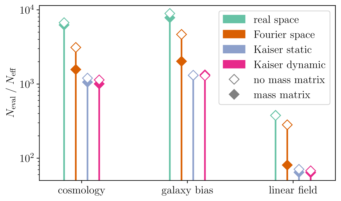
3.3 Conditioning strategies
From this point onward, we focus on the MCLMC sampler, using it to benchmark four preconditioning strategies outlined in section 2.3, both with and without diagonal mass matrix tuning. As in the previous section, we verify that all resulting posteriors are consistent before reporting performance metrics.
| Strategy | |||
|---|---|---|---|
| Best | 1005 | 879 | 390 |
| w/o mass matrix | 1136 | 883 | 518 |
| w/o dynamic | 1200 | 2256 | 579 |
| w/o Kaiser | 3112 | 3314 | 1395 |
| w/o Fourier | 6714 | 5504 | 1391 |
Figure 6 presents the number of model evaluations per effective sample for each conditioning strategy and set of parameters. As expected, sampling in real space performs the worse, since voxels can be highly correlated. This strong correlation also limits the potential efficiency gains from diagonal mass matrix tuning, as reflected in the small improvement observed in that case.
In contrast, sampling in Fourier space is expected to largely decorrelate the sampled parameters. Although naive prior-conditioning in Fourier space can still lead to poor conditioning, since different scales are not equally constrained, it enables significant improvement when combined with diagonal mass matrix tuning. Even better performance is achieved through preconditioning in Fourier space using a static Kaiser model, which appears to capture nearly all the diagonal conditioning benefits of Fourier space, as indicated by the minimal additional gain from mass matrix tuning. Finally, preconditioning with a dynamic Kaiser model performs only slightly better, likely because cosmology and bias parameters are sufficiently constrained in our setup, making the conditioning of the linear field weakly sensitive to their variations. For MCLMC in particular, better conditioning correlates with greater stability in numerical integration, allowing larger step sizes for the same nominal EEVPD, thereby enhancing sampling efficiency.
All metrics for the cosmological parameters are reported in table 2. The ground-truth values used for computing MSEs are obtained from a long NUTS sampling run, which is asymptotically unbiased. The metrics are consistent, with both and values of the same order, indicating no detectable bias in MCLMC sampling. Ultimately, we demonstrate that effective conditioning can improve sampling efficiency by approximately a factor of ten.
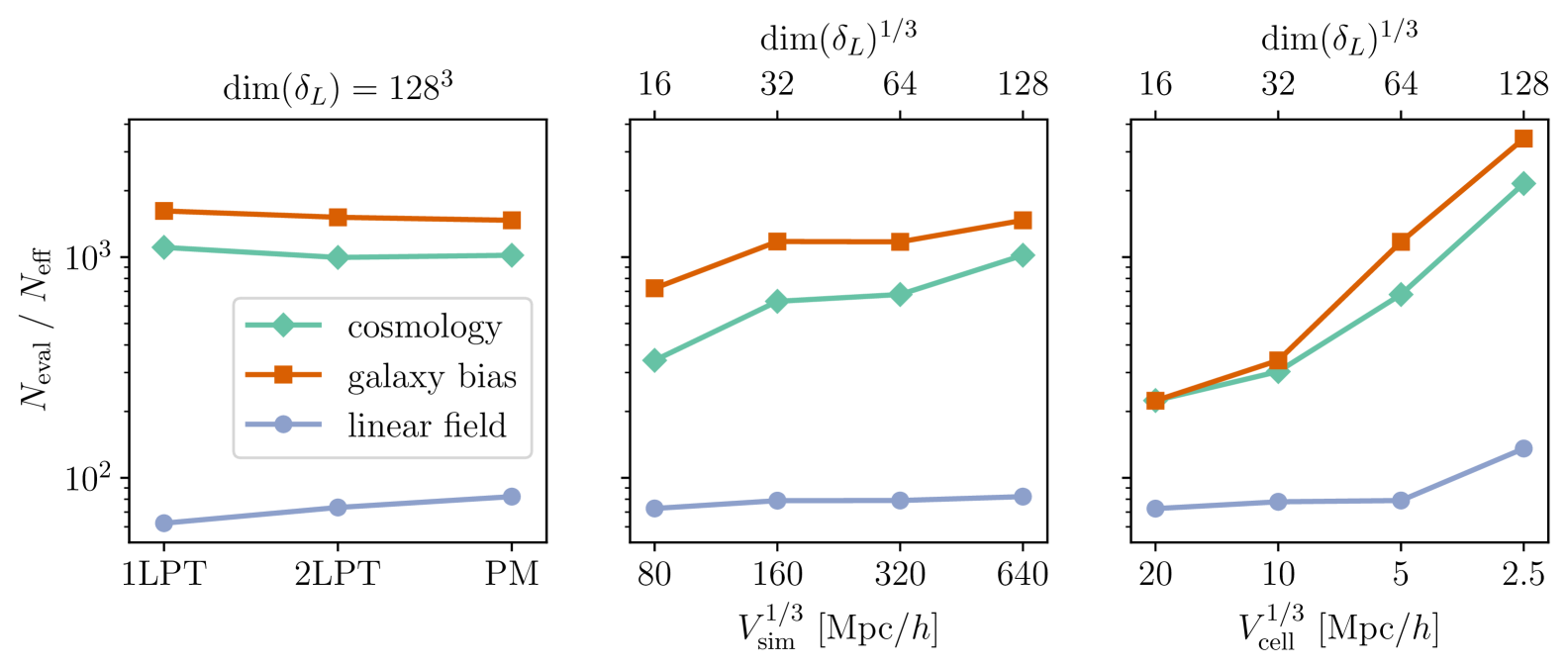
3.4 Scaling effects
Now that we have more insights into the performance of MCMC samplers and conditioning strategies for field-level inference, we aim to fully assess their applicability to upcoming galaxy surveys. In particular, we are interested in the scalability of MCLMC sampling with respect to dimensionality and modeling complexity.
Figure 7 (left panel) shows the number of model evaluations per effective sample for various LSS formation models (1LPT, 2LPT and PM) at a fixed volume of and voxel resolution of (hence ). We observe that in this setting, the sampling efficiency is largely independent of the complexity of the LSS formation model. Notably, we recover a similar magnitude in sampling efficiency as presented in [34] (below and for linear field and cosmology respectively). One may notice a slight increase in the sampling cost of the linear field, which could be attributed to the increased non-linearity of the forward model for LSS formation.
Figure 7 (middle panel) shows the same metric for different volumes, at a fixed voxel resolution of with the PM formation model. We observe almost no increase in the sampling cost of the linear field with respect to dimensionality. Since increasing the volume at fixed resolution primarily adds independent wavevectors to infer from, this corroborates the theoretical expectation that MCLMC efficiency remains independent of dimension for product densities. However, for cosmological and bias parameters, we note a slight increase in sampling cost with dimensionality, approximately scaling as . This is possibly related to the growing constraining power on these parameters, which reveals non-trivial correlations.
This effect is more pronounced when increasing resolution instead of volume. Figure 7 (right panel) shows sampling efficiency at a fixed volume of and varying resolutions. We observe a clear increase in sampling cost with dimensionality, approximately scaling as for cosmological and bias parameters. This indicates that field-level inference can become intrinsically more challenging at non-linear scales.
We must note that all these results are obtained for a mean galaxy density of , which is half the value used in previous sections and therefore yields twice the observational variance. This choice was made because, with the previously considered density of we found that for large volumes or high resolution and for the PM model only, the posterior exhibits some multimodality, with the chains getting stuck in different local modes171717We further checked this with a NUTS sampling run in case this was due to a MCLMC bias. (local in the sense that some modes admit visibly lower density values than others). In practice, this problem could be addressed in several ways: (i) adopting an annealing or tempering strategy (as performed in [67, 27]) to help the chains converge to or navigate between global modes; (ii) smoothing or noising the observations (at the cost of reducing constraining power). We think the first option would make fair comparisons more difficult in this benchmark, and that it is worth being benchmarked on its own. Therefore, we opted for introducing more observational noise (remaining within the typical galaxy density range of current spectroscopic surveys) to focus on the general scalability aspects of the problem.
On an indicative basis, with our best sampler and conditioning strategy, in the most computational intensive setting ( with 5-step PM displacement), a complete posterior can be obtained in less than 4 hours on a 8GB GPU node. For the same setting and conditioning strategy, NUTS took more than 80 hours.
4 Conclusion
We have benchmarked various state-of-the-art samplers for field-level cosmological inference from galaxy redshift surveys, emphasizing the critical role of preconditioning latent variables, particularly the initial density field, . We find that Fourier-space sampling of , combined with a linear rescaling which assumes a simple Kaiser model, improves sampling efficiency by an order-of-magnitude compared to naive real-space sampling. In this setup, tuning the mass matrix provides only marginal additional gains. However, we note that for real survey applications where observational noise varies across the footprint, this preconditioning may need refinement, and mass matrix tuning could become more relevant.
Among the samplers tested (HMC, NUTS, NUTS within Gibbs, MAMS, and MCLMC), the recently proposed MCLMC achieves the highest efficiency, outperforming other methods by approximately an order-of-magnitude. This gain mostly arises from MCLMC being run unadjusted, at the cost of introducing a potential bias in the cosmological posterior. However, this bias can be effectively controlled and reduced to negligible levels with a modest number of additional sampling steps. For a relevant modeling at reasonable scales ( with a PM scheme and 2nd order Lagrangian bias), MCLMC typically requires model evaluations per effective sample, mildly dependent of problem dimensionality, making it highly scalable for real-data applications. Nonetheless, we see that extending the inference to smaller physical scales may degrade efficiency, potentially requiring the use of tempering strategies to maintain robust performance. Similar complication may arise when considering more accurate small-scale modeling.
The benchmark code is publicly available181818github.com/hsimonfroy/benchmark-field-level and is intended to serve as a basis for future comparisons of alternative sampling methods. The forward model will be regularly augmented, in line with JaxPM developments, including the forthcoming implementation of massively parallel FFT calculations191919github.com/DifferentiableUniverseInitiative/jaxDecomp and improvements in the redshift-space galaxy density modeling.
Applying these methods to real survey data will indeed require additional developments, including a proper light-cone model, refined galaxy-matter connection at the relevant scales in redshift space, and the incorporation of survey selection and observational systematics. These enhancements will be the focus of future work.
Acknowledgments
The authors thank Marco Bonici and Natalia Porqueres for thoughtful discussions on field-level inference, and Wassim Kabalan for valuable insights on numerical implementation with JAX. They are especially grateful to Adrian Bayer for his constructive feedback and helpful comments on the manuscript. This work was granted access to the HPC resources of IDRIS under the allocations 2024-AD010414933 and 2025-475 AD010414933R1 made by GENCI.
Appendix A Hamiltonian formulation of the isokinetic Langevin dynamics
Here we show that we can rederive from an Hamiltonian the MCLMC equations of motion [49], without resorting to a momentum-dependent time rescaling used in [47, 48]. We follow the idea of [46] and consider a particle of position , momentum , and mass matrix , evolving in a -variate potential , with the Gaussian IsoKinetic (GIK) Hamiltonian
| (A.1) |
where and is a constant. Note that the adjective Gaussian in GIK refers to Gauss’s principle of least constraint, rather than to the Gaussian distribution.
Setting the auxiliary momentum and initial energy , we obtain from energy conservation that the kinetic energy is . For the canonical phase state , Hamilton equations are then
| (A.2) |
which translates for state into
| (A.3) |
This dynamics trivially admits the microcanonical ensemble as a stationary density. Moreover, when starting at kinetic energy , i.e. , this ensemble coincides with the isokinetic ensemble [46]
| (A.4) |
In particular, if ergodicity holds, the particle position samples the potential at the effective temperature . Therefore, by replacing by , setting , and adding Gaussian white noise as in [49], we recover the desired isokinetic Langevin equations 2.9 that sample from .
Appendix B Handling bias in unadjusted Langevin dynamics
In section 3.2, we showed that unadjusted MCLMC can efficiently provide posterior samples without noticeable bias. Here, we illustrate the biased behavior of MCLMC with a poor choice of step size, or equivalently an inappropriate Energy Error Variance Per Dimension (EEVPD) threshold.
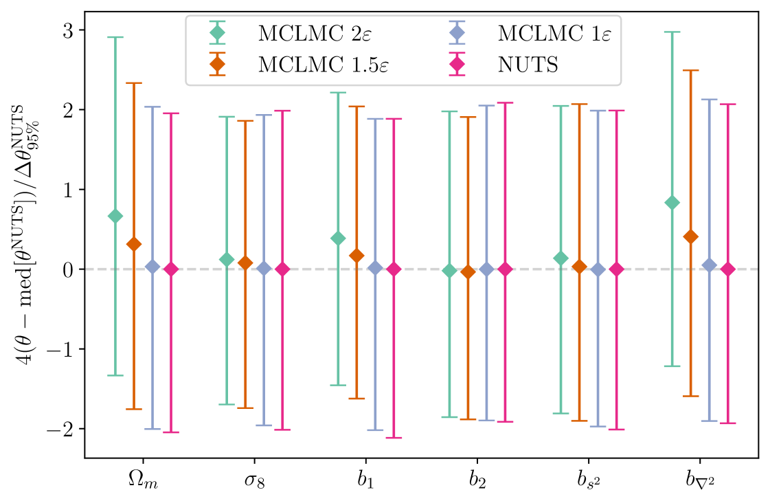
Figure 8 compares the posterior distributions of cosmological and bias parameters obtained from MCLMC with different step sizes to those obtained from NUTS, which is adjusted and therefore asymptotically unbiased. The model and sampler configurations are identical to those in section 3.2. We observe that our chosen EEVPD threshold of produces median and credible interval estimates nearly identical to those from NUTS, with differences likely dominated by Monte Carlo error. However, when using step sizes that are or larger, a clear bias appears in the estimation of some parameters, particularly , , and .
We showed in section 3.2 that for high-dimensional applications, NUTS is a magnitude less efficient than MCLMC, making it unsuitable for testing potential MCLMC bias. As a best practice, we recommend performing MCLMC sampling with at least two different EEVPD values, e.g. and , and checking for convergence of the posterior for the parameters of interest. Based on our experiments, once we identified an appropriate EEVPD threshold for our field-level inference problem (including preconditioning), we did not need to tune it further across the different settings considered in section 3.4.
References
- [1] DESI Collaboration, A.G. Adame, J. Aguilar, S. Ahlen, S. Alam, G. Aldering et al., Validation of the Scientific Program for the Dark Energy Spectroscopic Instrument, AJ 167 (2024) 62 [2306.06307].
- [2] Euclid Collaboration, Y. Mellier, Abdurro’uf, J.A. Acevedo Barroso, A. Achúcarro, J. Adamek et al., Euclid. I. Overview of the Euclid mission, arXiv e-prints (2024) arXiv:2405.13491 [2405.13491].
- [3] LSST Science Collaboration, P.A. Abell, J. Allison, S.F. Anderson, J.R. Andrew, J.R.P. Angel et al., LSST Science Book, Version 2.0, arXiv e-prints (2009) arXiv:0912.0201 [0912.0201].
- [4] DESI Collaboration, A.G. Adame, J. Aguilar, S. Ahlen, S. Alam, D.M. Alexander et al., DESI 2024 V: Full-Shape Galaxy Clustering from Galaxies and Quasars, arXiv e-prints (2024) arXiv:2411.12021 [2411.12021].
- [5] C. Hahn, P. Lemos, L. Parker, B. Régaldo-Saint Blancard, M. Eickenberg, S. Ho et al., : The First Cosmological Constraints from Non-Gaussian and Non-Linear Galaxy Clustering, arXiv e-prints (2023) arXiv:2310.15246 [2310.15246].
- [6] Beyond-2pt Collaboration, :, E. Krause, Y. Kobayashi, A.N. Salcedo, M.M. Ivanov et al., A Parameter-Masked Mock Data Challenge for Beyond-Two-Point Galaxy Clustering Statistics, arXiv e-prints (2024) arXiv:2405.02252 [2405.02252].
- [7] N.S. Sugiyama, D. Yamauchi, T. Kobayashi, T. Fujita, S. Arai, S. Hirano et al., New constraints on cosmological modified gravity theories from anisotropic three-point correlation functions of BOSS DR12 galaxies, MNRAS 523 (2023) 3133 [2302.06808].
- [8] O.H.E. Philcox and M.M. Ivanov, BOSS DR12 full-shape cosmology: CDM constraints from the large-scale galaxy power spectrum and bispectrum monopole, Phys. Rev. D 105 (2022) 043517 [2112.04515].
- [9] D. Zürcher, J. Fluri, R. Sgier, T. Kacprzak, M. Gatti, C. Doux et al., Dark energy survey year 3 results: Cosmology with peaks using an emulator approach, MNRAS 511 (2022) 2075 [2110.10135].
- [10] S. Nadathur, P.M. Carter, W.J. Percival, H.A. Winther and J.E. Bautista, Beyond BAO: Improving cosmological constraints from BOSS data with measurement of the void-galaxy cross-correlation, Phys. Rev. D 100 (2019) 023504 [1904.01030].
- [11] A.J. Hawken, M. Aubert, A. Pisani, M.-C. Cousinou, S. Escoffier, S. Nadathur et al., Constraints on the growth of structure around cosmic voids in eBOSS DR14, J. Cosmology Astropart. Phys 2020 (2020) 012 [1909.04394].
- [12] E. Paillas, C. Cuesta-Lazaro, W.J. Percival, S. Nadathur, Y.-C. Cai, S. Yuan et al., Cosmological constraints from density-split clustering in the BOSS CMASS galaxy sample, MNRAS 531 (2024) 898 [2309.16541].
- [13] M. Pinon, A. de Mattia, É. Burtin, V. Ruhlmann-Kleider, S. Codis, E. Paillas et al., A theoretical approach to density-split clustering, arXiv e-prints (2025) arXiv:2501.14638 [2501.14638].
- [14] G. Valogiannis, S. Yuan and C. Dvorkin, Precise cosmological constraints from BOSS galaxy clustering with a simulation-based emulator of the wavelet scattering transform, Phys. Rev. D 109 (2024) 103503 [2310.16116].
- [15] S. Codis, C. Pichon, F. Bernardeau, C. Uhlemann and S. Prunet, Encircling the dark: constraining dark energy via cosmic density in spheres, Monthly Notices of the Royal Astronomical Society 460 (2016) 1549.
- [16] W. Liu, A. Jiang and W. Fang, Probing massive neutrinos with the Minkowski functionals of the galaxy distribution, J. Cosmology Astropart. Phys 2023 (2023) 037 [2302.08162].
- [17] A. Jiang, W. Liu, W. Fang, B. Li, C. Barrera-Hinojosa and Y. Zhang, Minkowski functionals of large-scale structure as a probe of modified gravity, Phys. Rev. D 109 (2024) 083537 [2305.04520].
- [18] A. Banerjee and T. Abel, Nearest neighbour distributions: New statistical measures for cosmological clustering, MNRAS 500 (2021) 5479 [2007.13342].
- [19] A. Ouellette and G. Holder, Cosmological information content of Betti curves and -nearest neighbor distributions, arXiv e-prints (2025) arXiv:2502.09709 [2502.09709].
- [20] P. Villanueva-Domingo and F. Villaescusa-Navarro, Learning Cosmology and Clustering with Cosmic Graphs, ApJ 937 (2022) 115 [2204.13713].
- [21] G. Lavaux, J. Jasche and F. Leclercq, Systematic-free inference of the cosmic matter density field from SDSS3-BOSS data, arXiv e-prints (2019) arXiv:1909.06396 [1909.06396].
- [22] S. Duane, A.D. Kennedy, B.J. Pendleton and D. Roweth, Hybrid Monte Carlo, Physics Letters B 195 (1987) 216.
- [23] R. Neal, MCMC Using Hamiltonian Dynamics, 2011. 10.1201/b10905.
- [24] J. Bradbury, R. Frostig, P. Hawkins, M.J. Johnson, C. Leary, D. Maclaurin et al., JAX: composable transformations of Python+NumPy programs, 2018.
- [25] J. Jasche and B.D. Wandelt, Bayesian physical reconstruction of initial conditions from large-scale structure surveys, MNRAS 432 (2013) 894 [1203.3639].
- [26] J. Jasche and G. Lavaux, Physical Bayesian modelling of the non-linear matter distribution: New insights into the nearby universe, A&A 625 (2019) A64 [1806.11117].
- [27] N. Porqueres, O. Hahn, J. Jasche and G. Lavaux, A hierarchical field-level inference approach to reconstruction from sparse Lyman- forest data, A&A 642 (2020) A139 [2005.12928].
- [28] S.S. Boruah, E. Rozo and P. Fiedorowicz, Map-based cosmology inference with lognormal cosmic shear maps, MNRAS 516 (2022) 4111 [2204.13216].
- [29] N. Porqueres, A. Heavens, D. Mortlock, G. Lavaux and T.L. Makinen, Field-level inference of cosmic shear with intrinsic alignments and baryons, arXiv e-prints (2023) arXiv:2304.04785 [2304.04785].
- [30] N.-M. Nguyen, F. Schmidt, B. Tucci, M. Reinecke and A. Kostić, How Much Information Can Be Extracted from Galaxy Clustering at the Field Level?, Phys. Rev. Lett. 133 (2024) 221006 [2403.03220].
- [31] M.D. Hoffman, A. Gelman et al., The no-u-turn sampler: adaptively setting path lengths in hamiltonian monte carlo., J. Mach. Learn. Res. 15 (2014) 1593.
- [32] J. Zeghal, D. Lanzieri, F. Lanusse, A. Boucaud, G. Louppe, E. Aubourg et al., Simulation-Based Inference Benchmark for LSST Weak Lensing Cosmology, arXiv e-prints (2024) arXiv:2409.17975 [2409.17975].
- [33] B. Horowitz and Z. Lukic, Differentiable Cosmological Hydrodynamics for Field-Level Inference and High Dimensional Parameter Constraints, arXiv e-prints (2025) arXiv:2502.02294 [2502.02294].
- [34] A.E. Bayer, U. Seljak and C. Modi, Field-Level Inference with Microcanonical Langevin Monte Carlo, in 40th International Conference on Machine Learning, 7, 2023 [2307.09504].
- [35] N.-M. Nguyen, F. Schmidt, G. Lavaux and J. Jasche, Impacts of the physical data model on the forward inference of initial conditions from biased tracers, J. Cosmology Astropart. Phys 2021 (2021) 058 [2011.06587].
- [36] A. Kostić, N.-M. Nguyen, F. Schmidt and M. Reinecke, Consistency tests of field level inference with the EFT likelihood, J. Cosmology Astropart. Phys 2023 (2023) 063 [2212.07875].
- [37] D. Phan, N. Pradhan and M. Jankowiak, Composable Effects for Flexible and Accelerated Probabilistic Programming in NumPyro, arXiv e-prints (2019) arXiv:1912.11554 [1912.11554].
- [38] D.J. Eisenstein and W. Hu, Baryonic Features in the Matter Transfer Function, ApJ 496 (1998) 605 [astro-ph/9709112].
- [39] J.-E. Campagne, F. Lanusse, J. Zuntz, A. Boucaud, S. Casas, M. Karamanis et al., JAX-COSMO: An End-to-End Differentiable and GPU Accelerated Cosmology Library, The Open Journal of Astrophysics 6 (2023) 15 [2302.05163].
- [40] C. Modi, F. Lanusse and U. Seljak, FlowPM: Distributed TensorFlow implementation of the FastPM cosmological N-body solver, Astronomy and Computing 37 (2021) 100505 [2010.11847].
- [41] C. Rampf, F. List and O. Hahn, BULLFROG: multi-step perturbation theory as a time integrator for cosmological simulations, J. Cosmology Astropart. Phys 2025 (2025) 020 [2409.19049].
- [42] Y. Feng, M.-Y. Chu, U. Seljak and P. McDonald, FASTPM: a new scheme for fast simulations of dark matter and haloes, MNRAS 463 (2016) 2273 [1603.00476].
- [43] T. Matsubara, Nonlinear perturbation theory with halo bias and redshift-space distortions via the Lagrangian picture, Phys. Rev. D 78 (2008) 083519.
- [44] C. Modi, S.-F. Chen and M. White, Simulations and symmetries, MNRAS 492 (2020) 5754 [1910.07097].
- [45] H. Zhang, M. Bonici, A. Rocher, W.J. Percival, A. de Mattia, J.N. Aguilar et al., Enhancing DESI DR1 Full-Shape analyses using HOD-informed priors, arXiv e-prints (2025) arXiv:2504.10407 [2504.10407].
- [46] G.P. Morriss and C.P. Dettmann, Thermostats: Analysis and application, Chaos: An Interdisciplinary Journal of Nonlinear Science 8 (1998) 321.
- [47] G.V. Steeg and A. Galstyan, Hamiltonian Dynamics with Non-Newtonian Momentum for Rapid Sampling, in Advances in Neural Information Processing Systems, 2021.
- [48] J. Robnik, G. Luca, E. Silverstein and U. Seljak, Microcanonical Hamiltonian Monte Carlo, J. Mach. Learn. Res. (2022) .
- [49] J. Robnik and U. Seljak, Fluctuation without dissipation: Microcanonical Langevin Monte Carlo, in Proceedings of the 6th Symposium on Advances in Approximate Bayesian Inference, pp. 111–126, PMLR, 2024.
- [50] R.I. McLachlan, On the Numerical Integration of Ordinary Differential Equations by Symmetric Composition Methods, SIAM Journal on Scientific Computing (1995) .
- [51] S. Geman and D. Geman, Stochastic relaxation, gibbs distributions, and the bayesian restoration of images, IEEE Transactions on Pattern Analysis and Machine Intelligence PAMI-6 (1984) 721–741.
- [52] J. Robnik, R. Cohn-Gordon and U. Seljak, Metropolis Adjusted Microcanonical Hamiltonian Monte Carlo, arXiv e-prints (2025) arXiv:2503.01707 [2503.01707].
- [53] A. Mijatović, V. Mramor and G. Uribe Bravo, A note on the exact simulation of spherical brownian motion, Statistics & Probability Letters 165 (2020) 108836.
- [54] A. Durmus and A. Eberle, Asymptotic bias of inexact Markov chain Monte Carlo methods in high dimension, The Annals of Applied Probability 34 (2024) 3435.
- [55] J. Robnik and U. Seljak, Controlling the asymptotic bias of the unadjusted (Microcanonical) Hamiltonian and Langevin Monte Carlo, arXiv e-prints (2024) arXiv:2412.08876 [2412.08876].
- [56] O. Papaspiliopoulos, G.O. Roberts and M. Sköld, A general framework for the parametrization of hierarchical models, Statistical Science 22 (2007) .
- [57] N. Kaiser, Clustering in real space and in redshift space, MNRAS 227 (1987) 1.
- [58] M. Girolami and B. Calderhead, Riemann Manifold Langevin and Hamiltonian Monte Carlo Methods, Journal of the Royal Statistical Society Series B: Statistical Methodology 73 (2011) 123.
- [59] S. Livingstone, M. Faulkner and G. Roberts, Kinetic energy choice in hamiltonian/hybrid monte carlo, Biometrika 106 (2017) .
- [60] A. Cabezas, A. Corenflos, J. Lao, R. Louf, A. Carnec, K. Chaudhari et al., BlackJAX: Composable Bayesian inference in JAX, arXiv e-prints (2024) arXiv:2402.10797 [2402.10797].
- [61] D. Vats and C. Knudson, Revisiting the Gelman–Rubin Diagnostic, Statistical Science 36 (2021) 518 .
- [62] M.J. Betancourt, S. Byrne and M. Girolami, Optimizing The Integrator Step Size for Hamiltonian Monte Carlo, arXiv e-prints (2014) arXiv:1411.6669 [1411.6669].
- [63] Q. Jiang, On the dissipation of ideal Hamiltonian Monte Carlo sampler, Stat 12 (2023) e629.
- [64] S. Blanes, F. Casas and J.M. Sanz-Serna, Numerical Integrators for the Hybrid Monte Carlo Method, SIAM Journal on Scientific Computing 36 (2014) A1556 [1405.3153].
- [65] I.P. Omelyan, I.M. Mryglod and R. Folk, Symplectic analytically integrable decomposition algorithms: classification, derivation, and application to molecular dynamics, quantum and celestial mechanics simulations, Computer Physics Communications 151 (2003) 272.
- [66] T. Takaishi and P. de Forcrand, Testing and tuning symplectic integrators for the hybrid Monte Carlo algorithm in lattice QCD, Phys. Rev. E 73 (2006) 036706 [hep-lat/0505020].
- [67] A.E. Bayer, C. Modi and S. Ferraro, Joint velocity and density reconstruction of the Universe with nonlinear differentiable forward modeling, J. Cosmology Astropart. Phys 2023 (2023) 046 [2210.15649].