Semiclassical approximation for barrier billiards
Abstract
Barrier billiards are simple examples of pseudo-integrable models which form an appealing but poorly investigated subclass of dynamical systems. The paper examines the semiclassical limit of the exact quantum transfer operator for barrier billiards constructed in [J. Phys. A: Math. Theor. 55, 024001 (2022)]. The obtained asymptotic expressions are used to provide analytical arguments to support the conjecture that spectral statistical properties of barrier billiards are described by the semi-Poisson distribution and to derive the trace formulas for such billiards which in the transfer operator approach is not automatic.
I Introduction
The relationship between classical dynamics and statistical properties of corresponding quantum problems is the central topic of quantum chaos. The principal conjectures in this field depict only two limiting cases: (i) Quantum eigenenergies of typical classically integrable systems are statistically independent and well described by the Poisson distribution [1], (ii) Quantum eigenenergies of generic classically chaotic systems are strongly correlated and their correlation functions agree with those of standard random matrix ensembles depended only on system symmetries [2, 3].These conjectures are well accepted and were numerically checked in a huge variety of different problems.
However there exist models which are neither integrable nor chaotic and, consequently, they are not covered by the above conjectures. A characteristic example of such models is the so-called pseudo-integrable billiards (see, e.g., [4]) which are two-dimensional polygonal billiards whose all angles are rational multiplies of .
From numerous numerical calculations (see, e.g., [5]-[11], besides others) it was observed that the spectral statistics of pseudo-integrable billiards differs from the above mentioned universal statistics but is similar to spectral statistical properties of the Anderson model at the metal-insulator point [12, 13]. That type of statistics coined the name of intermediate statistics and is characterised by the following properties:
-
•
Level repulsion as for standard random matrix ensembles.
-
•
Exponential decrease of nearest-neighbour level distributions as for the Poisson statistics.
-
•
Non-trivial value of the spectral compressibility.
-
•
Fractal properties of eigenfunctions (in the Fourier space).
Analytical results in this field are rare and the majority of them is related with the calculation of the spectral compressibility by the summation over periodic orbits (cf., [9]).
Recently, a new analytical approach has been proposed in [14]-[16] to examine a specific example of pseudo-integrable billiards called barrier billiards which are rectangular billiards with a barrier inside (see Fig. 1(a)). The quantum problem consists in finding solutions of the Helmholtz equation
| (1) |
which obey the Dirichlet boundary conditions, , on the boundary of the rectangle and also along the barrier.

The method used in [14, 15] to investigate barrier billiards consists of two parts. First, two vertical billiard boundaries were removed and the problem was reduced to the scattering inside an infinite slab with a barrier parallel to slab boundary whose -matrix are exactly obtained by the Wiener-Hopf method. Second, to force eigenfunctions to be zero at the vertical boundaries special linear combinations of scattering solutions are constructed which, in the end, lead to the quantisation condition of the form
| (2) |
where is an exact transfer operator (cf. [18]) constructed from the scattering -matrix.
For simplicity, only symmetric barrier billiards with a barrier situated exactly at the middle of the rectangular are considered here. Due to the symmetry non-trivial solutions of such billiard correspond to a rectangular billiard with the height equal a half of the initial height but with different boundary conditions (partly Neumann, , and partly Dirichlet, ) along the upper boundary (see Fig. 1(b)). Formulas for general barrier billiards are more cumbersome (cf. [15]) and will not be discussed here.
For symmetric barrier billiards the scattering -matrix has the form [14]:
| (3) |
where
| (4) | |||
| (5) |
As it is usual in the Wiener-Hopf method [17], function is the result of the factorisation (with )
| (6) |
such that functions are free of zeros and singularities in, respectively, the upper half-plane and in the lower half-plane . A convenient explicit form of this function is [14]
| (7) |
The transfer matrix in this case is
| (8) |
Here and are, respectively, the lengths of the Neumann and the Dirichlet parts of the boundary (see Fig. (1)(b)). where is the length of the rectangle.
Though is given by an infinite (convergent) product, the moduli of are determined by a finite product
| (9) |
where are momenta of only propagating modes (i.e., with real momenta ) and the matrix restricted to these propagating modes is a finite unitary matrix of dimension as it should be for transfer operators [18].
The positivity of the right-hand side of expression (9) implies that real variables for propagating modes have to obey the following intertwining restrictions
| (10) |
For as in (8) these relations are automatic.
It was argued in [14] that phases in the -matrix generically can be considered as independent random variables which makes this matrix a random unitary matrix The main result of [14]-[16] is that the spectral statistics of barrier billiards in the semiclassical limit is independent of the position and the length of the barrier and is well described by the so-called semi-Poisson statistics with explicitly known correlation functions [7]
| (11) |
Here is the probability that two levels are separated by distance and inside this interval there exist exactly additional levels. is the two-point correlation function which determines the probability that two levels are at distance (with any numbers of levels inside). is the two-point form factor defined as the Fourier transform of
| (12) |
and is the spectral compressibility which determines the asymptotic behaviour of the variance of the number of levels, , in an interval
| (13) |
The goal of this paper is to examine the barrier billiard transfer operator in the semiclassical limit of high energies and to investigate a few related problems. Section II is devoted to the calculation of the transfer operator when and to the development of analytical arguments in favour of the statement that the spectral statistics of barrier billiards in this limit agrees with the semi-Poisson expressions. In Section III the semiclassical trace formula for barrier billiards is derived within the transfer operator approach. Surprisingly, the derivation is not straightforward. Certain technical questions are discussed in Appendices. Appendix A is devoted to the calculation of the infinite product (7) in the limit which permits to find the asymptotic expressions for all matrix elements of the -matrix (3). In Appendix B it is shown that these asymptotic values can be obtained by the direct summation of all images of the Sommerfeld diffraction on a half-plane. Properties of barrier billiard periodic orbits are studied in Appendix C.
II Barrier billiard and semi-Poisson statistics
Numerical calculations performed in [14, 15] for the unitary -matrix (8) with random phases and different choices of real coordinates obeying (10) (and, in particular, the ones specific for barrier billiards (4)) have demonstrated that spectral statistics of such -matrices are well described by the semi-Poisson distribution but it has not yet been confirmed analytically (except the calculation of the spectral compressibility in [16]).
In this Section three different random unitary matrices are considered. These matrices were chosen in such a way that they have the same form in the limit of large matrix dimension . One of these matrices is the -matrix (8) for propagating modes which describes the spectral statistics of barrier billiards.
The second unitary random matrix called below the -matrix is
| (14) |
is a rare example where one can prove that its statistics at large is the semi-Poisson one as it is a reduction of a random Lax matrix for an integrable Ruijsenaars-Schneider model [19, 20].
The third matrix called the -matrix is a block matrix () of the following form
| (15) |
Matrix is also a certain reduction of the Lax matrix of a Ruijsenaars-Schneider model [19, 20] but its spectral statistics is very different from statistics of matrix .
These three ensembles of random matrices have certain common points. First, they all are finite unitary matrices obtained by the multiplication of constant matrices by random phases. Second, without random phases all these matrices are symmetric real unitary matrices which implies that their eigenvalues are . Third, and the most important for our purposes, is that their limits exist and for all of them have the same block form
| (16) |
Such asymptotic equivalence together with certain additional considerations makes it reasonable that local spectral statistics of all three matrices in the limit are the same. As one of them is known to be described by the semi-Poisson distributions it follows (at least heuristically) that the two others (and, in particular, the barrier billiards) also have the same statistics.
II.1 Paraxial approximation
To find the transfer operator in the limit it is necessary to know the asymptotic value of . This function is given by the infinite convergent product (7) and standard calculations presented in Appendix A proved that when
| (17) |
From (5) it is possible to find all matrix elements of the scattering -matrix (3) (see (129)-(131)).
The key limit corresponds to the case (called here the paraxial approximation) when longitudinal momenta are large but their difference is small. It means that if and with not too close to then .
From the structure of the -matrix (3) and the definition of it follows that under such conditions and are but and are . Physically it means that we ignore the reflected waves and take into account only the transmitted waves.
From (129) one reads
| (18) |
The paraxial approximation consists in the assumption that . Then
| (19) |
Therefore in such approximation
| (20) |
As this result corresponds to small-angle scattering, it may also be obtained by an analog of the Fraunhofer diffraction. It means that this -matrix can be calculated simply by re-expansion of old (initial) wave functions into series of new functions (see also [16]). For symmetric barrier billiards of width initial (resp. final) normalised elementary solutions propagating in a slab with Neumann - Dirichlet (resp. Dirichlet - Dirichlet) boundary conditions are
| (21) |
Therefore in the paraxial approximation the -matrix are determines by the following expansion
| (22) |
Here it is taken into account that in such (paraxial) approximation longitudinal momenta are considered equal . In particular, it means that the normalisation of all solutions are the same.
One can further simplify this matrix by taking into account only the pole term
| (24) |
Let us re-arrange matrix elements of the -matrix by grouping together indices of the same parity so the full matrix has four blocks structure
| (25) |
As the -matrix is symmetric (the reciprocity principle) it means that in the paraxial approximation only elements are non-zero in the limit (or ) and the full -matrix has the form
| (26) |
This limiting paraxial -matrix is formally unitary as it comes from an expansion of one set of orthogonal functions into another set of orthogonal functions but the unitarity is achieved only provided the summation over intermediate states is done over all integers
| (27) |
It can be confirmed by usual formulas (with the symmetric summation over )
| (28) |
When matrix indices are finite the matrix is not unitary and its eigenvalues are not on the unit circle which makes the investigation of spectral statistics of the -matrix (8) in the paraxial approximation meaningless.
It is well understood that the linear decrease of matrix elements from the diagonal (as in (24)) is the principal ingredient of random matrix models with intermediate statistics [12, 13]. Therefore it is natural to conjecture (at least heuristically) that different models which have the same asymptotic behaviour of matrix elements should have the same local spectral statistics. Thus, to elucidate spectral correlation functions of the -matrix (i.e., barrier billiards) one could try to find a different matrix model with known statistical properties which have the same asymptotic as in (26).
II.2 Model A
Let us consider a seems to be unrelated matrix
| (29) |
where matrix depends on one free real parameter
| (30) |
Here
| (31) |
It appears that this matrix is the Lax matrix for a certain integrable compact Ruijsenaars-Schneider model [19, 20] such that are momenta of particles and are their coordinates. This matrix is meaningful provided that coordinates are such that and are of the same signs for all indices. Denote this allowed region of by . When matrices (30) and (29) are unitary matrices.
Due to the existence of integrable structure of action-angle variables in the considered Ruijsenaars-Schneider model [21]-[23] it is possible to prove [19, 20] that if phases (momenta) are uniformly distributed in the interval and are uniformly distributed in the region then eigenvalues of matrix in (29) (denoted below by ) are also uniformly distributed in . It means that the joint probability of eigenvalues of matrix (29) has the form
| (32) |
with a normalisation constant .
Contrary to the usual random matrix ensembles, no wronskians are presented in this expression. Nevertheless, the eigenvalue spectral statistics of such models is non-trivial due to the structure of allowed region . The explicit form of this variety depends strongly on and [19, 20]. The properties of only two special cases will be reminded here. For other cases consult [19, 20].
The first case corresponds to
| (33) |
For this value the -matrix takes the following form
| (34) |
It is easy to check that such matrix can be obtained from the above -matrix (3) after the substitution instead of real complex with real (an analog of the Wick rotation).
This matrix is unitary provided obey intertwining conditions similar to (10). Let be an ordered set of numbers with odd
| (35) |
then the allowed region of where matrix (34) is unitary is defined as follows
| (36) |
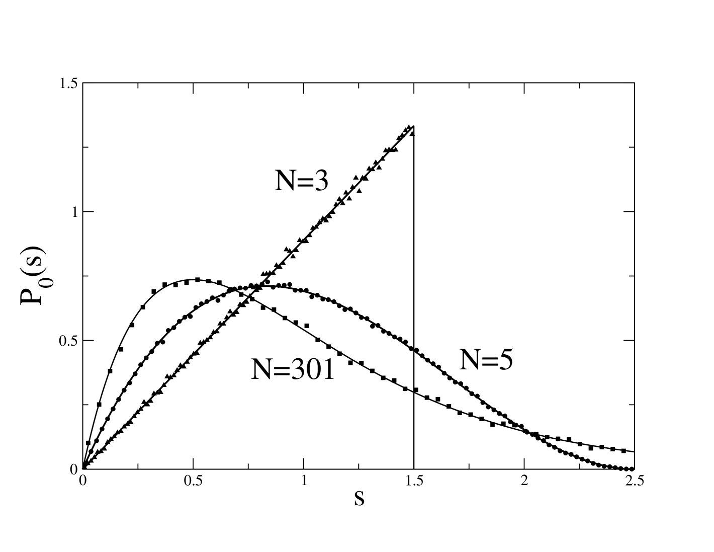
The simplicity of this region permits to find all local correlation functions of eigenvalue distribution (32) analytically even at finite (but odd) . For example, the nearest-neighbour distribution, , is the probability that two eigenvalues are at distance and there is no eigenvalues inside this interval. According to the definition of (see (36)) between any two near-by eigenvalues there exists another eigenvalue whose symmetric image has to be in-between these two. The integral of it is, evidently, . All other eigenvalues (together with symmetric images of even levels) should be ordered and to be in-between and . Therefore the integration over them is proportional to . Rescaling the eigenvalues to mean level density and impose the standard normalisations one proves that the nearest-neighbour distribution for matrix in (29) with finite is
| (37) |
Similar considerations prove that the probability, , that in the interval there exist exactly eigenvalues ()
| (38) |
where are binomial coefficients.
When with fixed these distributions tends to the known semi-Poisson expressions (11). For illustration, in Fig. 2(a) the results of numerical calculations for , , and are presented. It is clearly seen that the numerics confirm well the above formulas. The calculations were done in the following manner. First, points were independently and uniformly chosen in . Then the points were numerated according to ascendent order (cf. (35)). Finally, every even points were shifted by as required by (36).
a)
b)
The -matrix (8) which describes the barrier billiard also corresponds to a Ruijsenaars-Schneider model but to a non-compact one. No ’natural’ compactification of this model such that the resulting correlation functions are calculated analytically has not been found yet.
There exist several variants of the random integrable model (34) [20]. Using the condensation of measure theory (see, e.g., [32]) one can argue that for large almost all (but fixed) realisations of coordinates produce the -matrix (29) whose spectral statistics is well approximated by the semi-Poisson distributions (11). The simplest choice is
| (39) |
for which conditions (35) and (36) are automatically satisfied. Simple calculations show that for these coordinates and matrix denote, for clarity, by takes a particular simple form
| (40) |
After the multiplication by random phases one gets model A indicated in (14).
This matrix has appeared as a particular example of a quantisation of an interval-exchange map [33] and has been investigated in [34]. Such matrix with i.i.d. random phases, , is the simplest example of random matrix ensemble with the semi-Poisson statistics in the limit of large matrix dimension. Similar to the -matrix, matrix is a finite real unitary (i.e., orthogonal) symmetric matrix such that .
Consider now matrix (14) in the limit . It is clear that non-zero matrix elements of the -matrix are close to two diagonals . As has to be odd it means that formally
| (41) |
As it is the same as the limit of the -matrix (cf. (26)) one may conclude that spectral statistics of the -matrix (8) in the limit of large is well described by spectral statistics of the -matrix (14), i.e., the semi-Poisson statistics (11). This conclusion is based on the above (heuristic) conjecture that matrices with the the same asymptotic linear falloff of matrix elements have the same spectral properties in the limit of large matrix dimensions.
Strictly speaking, the above reasoning could be applied only for odd . The case of even matrix dimension requires modifications. It is plain that many unitary matrices may have the same asymptotic behaviour of matrix elements as in (26).
II.3 Model C
Consider again the matrix (30) but with a different value of parameter
| (42) |
It was shown in [20] that in this case the allowed region consists of points on a circle such that the differences between near-by points are larger than . A convenient representation of this region is the following
| (43) |
The joint probability of these points is given by (32) with the above definition of the allowed region. It is plain that correlation functions in such case correspond to the Poisson distribution but for ’thick’ points of the size .
Consider independent points uniformly distributed at interval of length . The probability that in an interval there are exactly points is given by the known Poisson distribution
| (44) |
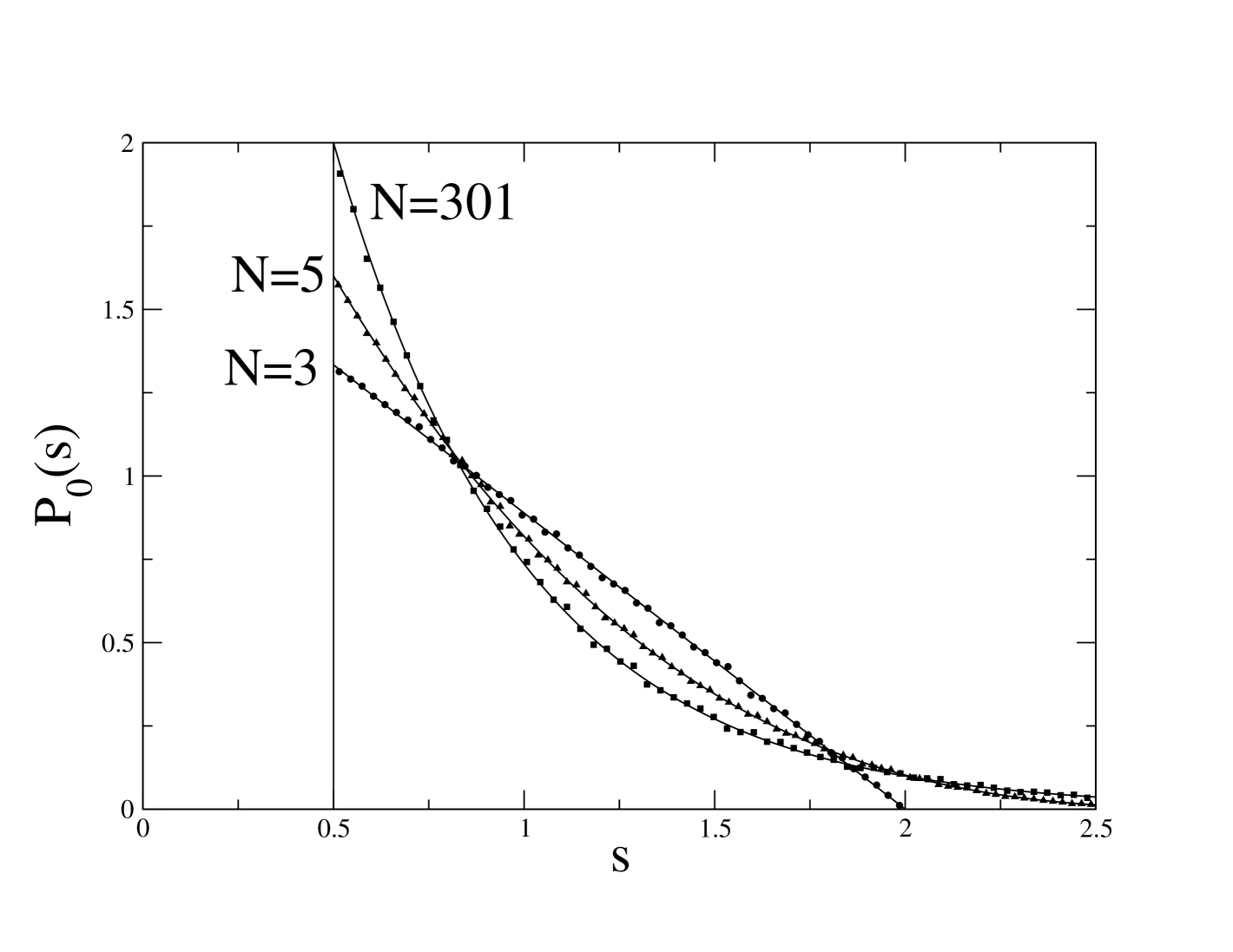
For the model eigenvalues of matrix (30) are uniformly distributed on the unit circle and after the unfolding the distribution of its eigenvalues are obtained from the above Poisson formulas with the shift: and . In the end one gets that the nearest-neighbour distributions for this model is
| (45) |
with the following restriction
| (46) |
When these nearest-neighbour distributions tend to the shifted Poisson distribution
| (47) |
Notice the very strong ’level repulsion’ (i.e., the absence of eigenvalues at small separations): for . For illustration, a few such examples are presented in Fig. 2(b).
As in previous Section consider a particular case with
| (48) |
Direct calculations shows that in this case matrix denote by takes the form
| (49) |
The matrix
| (50) |
is a unitary matrix and in the limit its spectral statistics tends to the shifted Poisson distribution (47).
It is these matrices that enter in the construction of block matrix in (15) for even . It is plain that in the limit the -matrix has the same asymptotic form as the above two models. Due to the block structure of the -matrix (15), the square of its eigenvalues are eigenvalues of the product of two independent matrices
| (51) |
where and are two independent sets of random variables uniformly distributed between and .
According to the above asymptotic equivalence conjecture spectral statistics of matrix has to be the semi-Poisson one. The results of numerical calculations of the nearest-neighbour distributions for this matrix are presented in Fig. 3. It is clearly seen that it is close to the semi-Poisson values (11). For completeness, in the Insert of this figure the nearest-neighbour distribution of one -matrix is presented together with the theoretical prediction (47).
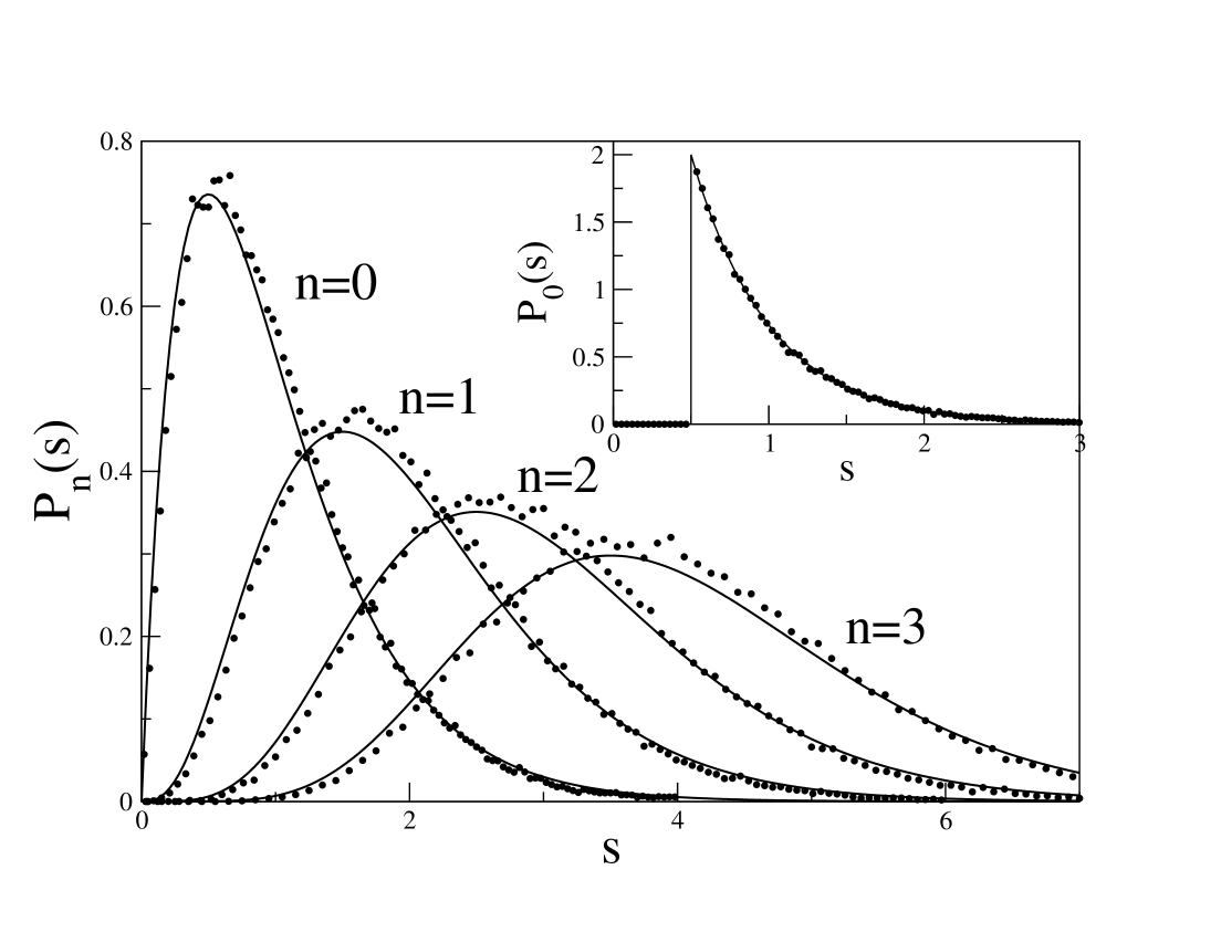
Careful discussion of spectral properties of products of certain matrices with intermediate statistics will be given somewhere.
III Trace formula for barrier billiards
Trace formulas are the main tool in the semiclassical approach to quantum problems [24]. Such formulas relate the density of quantum eigenenergies to a sum over classical periodic orbits of a given system. For pseudo-integrable billiards periodic orbits are organised in families of parallel rays restricted from the both sides by billiard edges and the trace formula for such models has the form [4]
| (52) |
where
| (53) |
and
| (54) |
Here the summation is done over all classical periodic orbits. is the periodic orbit length, is the area occupied by a given periodic orbit family, and is the phase factor related with billiard boundary conditions.
Only for special pseudo-integrable billiards these quantities can be calculated analytically (cf., [9]) but for the barrier billiard indicated in Fig. 1(b) their computation is straightforward. From Appendix C (see also Appendix D in [25]) it follows that for a primitive periodic orbit
| (55) | |||||
| (56) |
Within the transfer operator formalism the density of state can be expressed by standard arguments. From the quantisation condition (2) one concludes that formally (with )
| (57) |
The difference between the transfer operator discussed in the paper and the general theory of quantum maps (see, e.g.,[26]) lies in the definition of periodic orbits. In quantum maps periodic orbits are built from phases in the transfer matrices but in the barrier billiards periodic orbits are fixed geometrically (cf. (56)) and are not directly related with phases of the -matrix (8). As usual, the periodic orbit lengths for barrier billiards will reappear after the saddle-point summation but the determination of a non-trivial pre-factor proportional to the area occupied by a periodic orbit, in (56) within the transfer operator approach, seems, has not been discussed in the literature. The rest of this Section is devoted to such calculations.
The periodic orbits contribution is contained in terms with even powers of the -matrix (as only in such terms one can get terms). The trace includes the summation over even and odd indices. In Section III.1 it is demonstrated how to sum over all odd indices (which corresponds to waves started from the Dirichlet part of the billiard boundary) with fixed even indices. It is evident that the full trace is twice this value.
It will be shown below that for large
| (58) |
where function is even: .
Using the Poisson summation formula (corrections at small can be added if necessary)
| (59) |
where
| (60) |
For large this integral can be calculated by the saddle-point method. The saddle-point values of are determined from the condition which gives
| (61) |
with .
It is plain that is the action along the periodic orbit , is the length of this orbit, and is the momentum along this orbit.
Finally the contribution of (58) to the trace formula (a term with is requires a slightly different treatment)
| (62) |
The explicit calculation of function is performed in Section III.1 where it is shown that it is related to the trace of a certain matrix. Section III.2 is devoted to the calculation of eigenvalues of this matrix which, in the end, permit to prove that the transfer operator method leads to the correct answer for the trace formula.
III.1 Summation over odd indices
Let us calculate the trace of powers of the -matrix when only forward scattering are taken into account because as was indicated above the reflected waves are small at large momenta. One has
| (63) |
where
| (64) |
The factor appears because the fixation of odd indices and summation over even ones give exactly the same answer due to the cyclic invariance of the trace.
In the paraxial approximation (24) one needs to calculate the following sum
| (65) |
The presence of paraxial -matrix elements forces the summand to be close to external indices and
| (66) |
It will be shown that the summations over and converge which implies that for large and are small, and . Then the following expansions are justified
| (67) |
After these approximations one can sum over all which leads to the following expression (as )
| (68) |
where () and
| (69) |
When
| (70) |
For
| (71) |
Shifting in the second term gives
| (72) |
The summation in the above expressions corresponds to the sum over odd integers. As
| (73) |
the remaining sums can be calculated from known identities for the Bernoulli polynomials (see, e.g., [27])
| (74) |
and
| (75) |
Split into the sum of integer, , and fractional, , parts: with then
| (76) |
and
| (77) |
Finally
| (78) |
where and
| (79) |
Put the obtained expression (78) into general formula (63) and assume that all are close to each other
| (80) |
In such approximation there is only one large index and relatively small differences . Notice that and, consequently, depend only on . In the end one gets
| (81) |
where
| (82) |
The total phase in this expression is
| (83) |
The sum in (81) is exactly as in (58) and according to (62) its contribution to the trace formula in the saddle-point approximation reduces to the calculation of the value of at equals the saddle-point value (see (61))
| (84) |
It implies that in the saddle-point approximation
| (85) |
The phase factor in (83) takes the following value
| (86) |
As enters in the exponent (see (82)) the term can be omitted.
From this one concludes that the function is
| (87) |
where
| (88) |
By the construction function is independent on therefore the above equation can be rewritten in the form
| (89) |
with in (88) considered as matrix.
III.2 Eigenvalues of the -matrix
To calculate the trace in (89) it is necessary to find eigenvalues of matrix in the limit .
Consider a matrix
| (90) |
This matrix at finite determine the so-called discrete prolate spheroidal sequences whose properties were thoroughly investigated in [28].
The structure of eigenvalues and eigenfunctions of this matrix in the limit of can be found from the following simple considerations. Let us consider the identity (with an odd integer )
| (91) |
Functions (Greek letters are used to numerate eigenvalues)
| (92) |
are orthogonal when and the above expression signifies that the matrix in the right-hand side of Eq. (91) has eigenvalues equal and zero eigenvalues. For large the matrix in (91) tends to that in (90). Therefore, for matrix with also has asymptotically eigenvalues and zero eigenvalues (plus transitional eigenvalues between and [28]).
This all is valid when . The matrix is periodic in with period . When one has . Therefore if one defines then with this definition . As this matrix is conjugate to it has the same eigenvalues. Finally matrix
| (93) |
for all has asymptotically unit eigenvalues and zero eigenvalues.
matrix in (79) can be rewritten as follows
| (94) |
and, consequently, matrix has asymptotically eigenvalues equal and eigenvalues equal .
Let with denote eigenvalues of this matrix. One can arrange all eigenvalues in such a way that the first eigenvalues are and the rest are equal to . As we are working in the limit it is convenient to use a (quasi) continuous variable . Then the function can be written in the following form
| (95) |
Consider now the matrix (88) in the saddle-point approximation
| (96) |
The phase in this expression depends only on the fractional part of : with . For primitive periodic orbits and are co-prime integers, therefore, and are also co-prime integers.
The key point in the investigation of eigenvalues of matrix is the observation that any eigenfunction of matrix , , in (92) after the multiplication by phase factor with integer tends at large to another eigenfunction of the same matrix with, in general, a different eigenvalue. Indeed
| (97) |
One has
| (98) |
Therefore, the shift in the above expression differs from by a small amount in comparison to and (heuristically) can be ignored in the limit .
In the continuous approximation when variable is introduced (as in (95)) such shift corresponds to
| (99) |
Notice that for primitive periodic orbits integers and are co-prime and, consecutively. the sequence with wraps all fractions with . It means that the sequence of of eigenfunctions is closed under multiplications by .
These considerations show that an eigenfunction of matrix in (88) can in the limit be approximated by by the sum
| (100) |
where is any number in the interval . As in the continuous notations
| (101) |
the eigenvalue condition
| (102) |
implies that
| (103) |
Functions are orthogonal and this equation is equivalent to the following system of equations
| (104) |
Therefore, new eigenvalues are determined from the condition (here )
| (105) |
As all are equal to either or , which means that new eigenvalues are strongly degenerated and can take only different values (from the total number )
| (106) |
As for the prolate spheroidal sequences the number of eigenvalues which differ from the above values is small with respect to the matrix dimension which agrees well with numerical calculations.
To find the main quantity (87) it is necessary to know the value
| (107) |
where the sum is taken over all eigenvalues of matrix . From (105) it follows that almost all eigenvalues in the power in the limit can take only two values or depending on the sign of the product of over . It is convenient to rename variables: . To avoid the double counting new variable has to be chosen between and .
From (95) one gets
| (108) |
According to (95)
| (109) |
Split with into integer and fractional parts
| (110) |
Then it is plain that
| (111) |
which using (89) proves that
| (112) |
As one gets
| (113) |
Finally
| (114) |
which agrees with the direct calculation of the contribution of a primitive periodic orbit (cf. (56)) (the factor has been included in (62)).
IV Conclusion
The semiclassical limit of high energy of the transfer operator for symmetric barrier billiards proposed in [14] is calculated and two related topics are investigated.
The first concerns the spectral statistical properties of barrier billiards. By comparison of the asymptotic form of the transfer operator with the asymptotic of a certain class of random unitary matrices with known spectral statistics one concludes (at least heuristically) that spectral correlation functions of barrier billiards have to be described by the semi-Poisson formulas in a good agreement with numerical calculations.
The second subject consists in the derivation of the trace formula for barrier billiards within the transfer operator approach. Usually the semiclassical trace formulas are obtained from standard geometrical considerations but in the discussed method the calculations are not straightforward and require the knowledge of eigenvalues of certain unusual matrices. Albeit the answer was known in advance, the calculations reveal a new mechanism by which corrections to a saddle-point are combined to produce the pre-factor for the barrier billiard trace formula.
Though the calculations start from the exact transfer operator expression, it is demonstrated that the semiclassical limit of many quantities could be obtained from simple physical considerations which may open a way of analytical investigations of more general pseudo-integrable models and, in particular, of triangular billiards.
Appendix A Asymptotic calculations of
From Eq. (7) it follows that can be rewritten as two convergent products
| (115) |
The first product is known [27]
| (116) |
Here is Euler’s constant.
The second product can be expressed as follows (where it is implicit that )
| (117) |
This sum can be estimated by the Euler-Maclaurin summation formula
| (118) |
where are the Bernoulli numbers , , .
Though the integrals are elementary, for our purpose it is sufficient to approximate the difference for large and/or large by the first term of expansion
| (119) |
The summation over is substituted by two integrals one from to and the second from to which corresponds, respectively, to propagating and evanescent modes (in the last term (116) is used)
| (120) |
where
| (121) | |||||
| (122) |
The sign of the imaginary part () is fixed by the requirement that all singularities of are in the lower half-plane.
Combining all factors one gets
| (123) |
This asymptotic is valid for large and . The error is assumed to be .
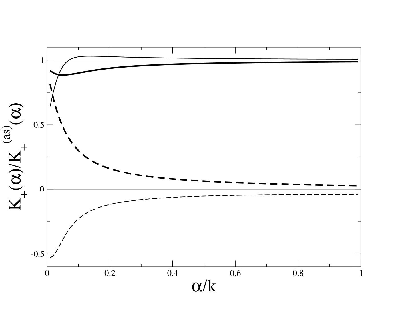
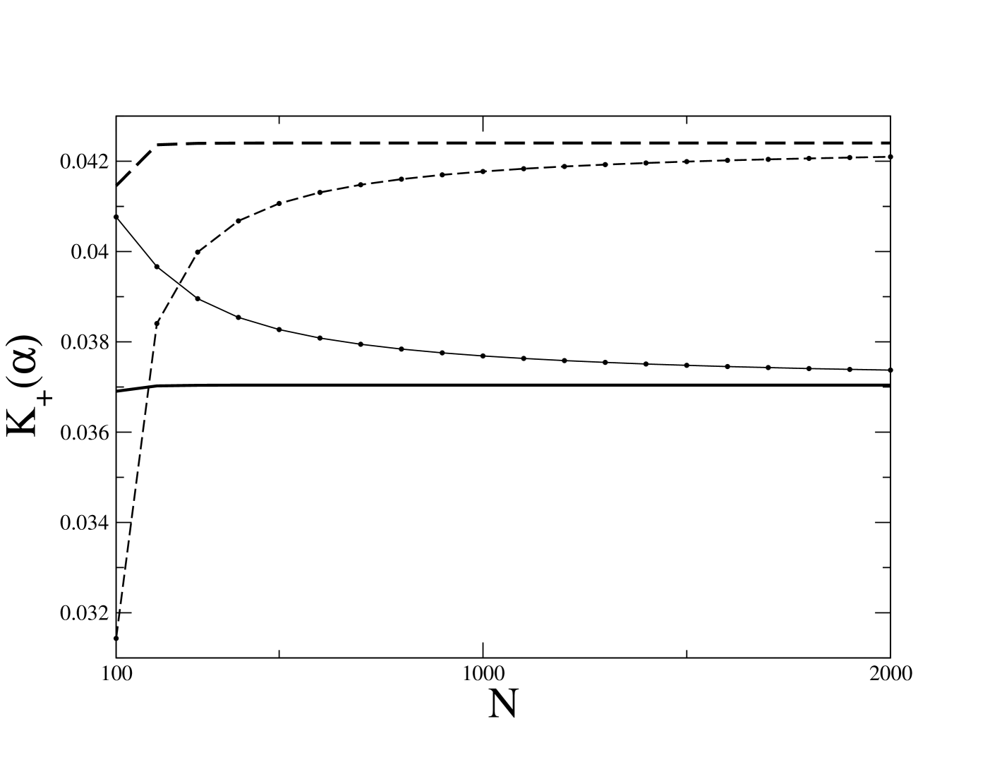
The ratio of calculated numerically to the asymptotic formula (123) is presented in Fig. 4(a). As expected, for not small values of the argument this ratio indeed is close to . Calculation of the behaviour of at small is beyond the scope of the paper.
a)
b)
As the transfer operator is exact it can be used also for numerical computations of the billiard barrier spectrum. In such a case it is of interest to find a convenient method of calculation of . By construction, the infinite product in (7) converges and may be calculated simply by the multiplication of a large number, , of factors (as it is done in Fig. 4(a)). But the error will be only . Better accuracy can be achieved by the approximation of the rest by the Euler-Maclaurin formula (118). One has
| (124) |
The correction term, , has the form (it is assumed that to fix the correct branches)
| (125) |
where . Take a few terms of the expansion of function at large
| (126) |
where
| (127) |
and calculate the necessary sums by the Euler-Maclaurin formula (118). In this way one obtains
| (128) |
At Fig. 4(b) it is shown that adding just the above three correction terms amplifies drastically the accuracy.
Appendix B Asymptotic of the -matrix by method of images
Asymptotic formula (123) permits to find the behaviour of the full propagating -matrix (3) at large momenta
| (129) | |||
| (130) | |||
| (131) |
The purpose of this Appendix is to demonstrate that these asymptotic values can be obtained from the well-known Sommerfeld solution for the diffraction on a half-plane [29, 30] .
Formally, for any diffraction problem the wave at large distances from the diffraction centre is the sum of an incident wave and a reflected wave. In two dimensions
| (132) |
where is a diffraction coefficient depended on the incident angle and the angle of reflection .
For the scattering on a barrier (i.e., a half-plane) Sommerfeld shows [29, 30] that
| (133) |
where all angles are calculated counterclockwise from the barrier (see Fig 5) .

A principal difficulty in treating pseudo-integrable billiards consists in the impossibility to split scattered waves into the sum of initial and final waves which manifests in the divergence of the corresponding diffraction coefficient in certain directions (called optical boundaries). For diffraction coefficient as in (133) optical boundaries appear at . Waves in vicinities of optical boundaries are complicated which lead to many unusual properties of pseudo-integrable billiards (cf. [31]).
The normalised incident wave for the barrier problem in the cartesian coordinates as in Fig. 5 is indicated in (21). This wave can be represented as the sum of two plane waves with incident angles
| (134) |
In a vicinity of the barrier tip the scattered wave takes the form
| (135) |
where is the value of the incident wave at the barrier tip (i.e., in Fig. 5)
| (136) |
and is the diffraction coefficient (133) with substitution (134)
| (137) |
After the scattering on the barrier tip there are two possibilities. If the wave will propagate between two horizontal boundaries with the Dirichlet boundary conditions. If the wave has to propagate in a tube with the Dirichlet condition on the lower boundary and the Neumann boundary on the upper boundary. In the both cases the field in a point with is the sum of all rays which connect the barrier tip with this point after multiple reflections on horizontal boundaries. These reflections correspond to all unfolded images of the final point: with integer .
Therefore, the distances between the tip and the final points are
| (138) |
Here is the smallest angle between the straight line passed through the barrier and the corresponding classical ray.
The total wave is the sum over all these rays. The transmitted field with is
| (139) |
It is clear that . The reflected field with is given by a sum
| (140) |
which obeys different boundary conditions: and .
The usual way of calculating such sums is to use the Poisson summation formula and the saddle-point method. For completeness, these calculations are present below.
Let then
| (141) |
The saddle-point value of is determined from the condition which leads to
| (142) |
Finally in the saddle-point approximation
| (143) |
This result implies that
| (144) |
By definition, the -matrix element is the coefficient in front of the normalised final function (cf. (21))
| (145) |
As and this result coincides with (129).
The reflected wave can be obtained similarly. The differences with the above formulas are the following. First, due to the factor in (140) one has to substitute which, in particular, implies that Eq. (144) has to be multiply by . Second, due to a different definition with and
| (146) |
Finally
| (147) |
which is the same as in (130).
Appendix C Contribution of a primitive periodic orbit in barrier billiards
Periodic orbits in barrier billiards form parallel periodic families (pencils) restricted from the both sides by singular points. Let us consider one periodic orbit which connects the origin (i.e., low-left corner of barrier billiard) with point of coordinates (see Fig. 1(b)) where and are two integers. For primitive orbits these integers have to be co-prime. In Fig. 1(b) it means that
| (148) |
and the equation of this orbit is
| (149) |
Singular vertices in the considered billiard (see Fig. 1(b)) after unfolding are situated in points with coordinates
| (150) |
with integers and .
It is well known (and can easily be checked by direct calculations) that the distance between a point with coordinates and a line determined by the equation is
| (151) |
(Different signs of correspond to points in different sides of the line.)
Therefore the distances between all singular points and the periodic orbit passed through the origin are
| (152) |
Denote , , and separating the integer and fractional parts of
| (153) |
one gets
| (154) |
As integers , are co-prime there exist two integers and such that . Therefore if and are of the same parity the minimum of the distances are equal to
| (155) |
and if and are of different parity then the minimal distances are
| (156) |
Finally the width of one periodic orbit channel (which includes an orbit through the origin) is
| (157) |
The total width of any periodic orbit family is and the second periodic orbit pencil has the width . As two channels correspond to periodic orbits with different total signs one concludes that the contribution of the above primitive periodic orbit is (taking into account the factor due to the implicit integration over the longitudinal coordinate.)
| (158) |
where is the phase factor (the Maslov index) of a periodic trajectory passed through the origin. This factor equals where is the number of crossings the Neumann parts of the boundary by the considered orbit. For the orbit which starts from the origin it can be found without calculations by the following arguments. Such orbit passes through the point which is the centre of the rectangle with sides and . It is plain that the bottom-left rectangle and the top-right rectangle are mirror images of each other. Therefore, the total number of intersections with Neumann boundaries inside these rectangles will be even. The only possibility to have odd numbers is the crossing the Neumann boundary exactly in the centre with coordinates but it is possible only when is even and is odd. As integers and are co-prime it means that when is even has to be automatically odd. Therefore, the phase is the follows
| (159) |
Final formula is obtained from (158)
| (160) |
It is independent on and depends only on .
References
- [1] M. V. Berry and M. Tabor, Level clustering in the regular spectrum, Proc. R. Soc. Lond. A 356, 375 (1977).
- [2] O. Bohigas, M. J. Giannoni, and C. Schmit, Characterization of chaotic quantum spectra and universality of level fluctuation laws, Phys. Rev. Lett. 52, 1 (1984).
- [3] M. L. Mehta, Random matrices, Third edition, Academic Press (2014).
- [4] P.J. Richens and M.V. Berry, Pseudointegrable systems in classical and quantum mechanics, Physica D: Nonlinear Phenomena 2, 495 (1981).
- [5] K. Życzkowski, Classical and quantum billiards: integrable, nonintegrable and pseudo-integrable, Acta Physica Polonica B 23, 245 (1992).
- [6] A. Shudo, Y. Shimizu, P. Šeba, J. Stein, H.-J. Stöckmann, Statistical properties of spectra of pseudointegrable systems, Phys. Rev. A, 49, 3748 (1994).
- [7] E. Bogomolny, U. Gerland, and C. Schmit, Short-range plasma model for intermediate spectral statistics, Eur. Phys. J. 19, 121 (2001).
- [8] J. Wiersig, Spectral properties of quantized barrier billiards, Phys. Rev. E 65, 046217 (2002).
- [9] E. Bogomolny, O. Giraud, and C. Schmit, Periodic orbits contribution to the 2-point correlation form factor for pseudo-integrable systems, Comm. Math. Phys. 222, 327 (2001).
- [10] Črt Lozej and E. Bogomolny, Intermediate spectral statistics of rational triangular quantum billiards, Phys. Rev. E 110, 024213 (2024).
- [11] V. Balasubramanian, R. Nath Das, J. Erdmenger, and Zhuo-Yu Xian, Chaos and integrability in triangular billiards, arXiv: 2407.11114 (2024).
- [12] B. L. Altshuler, I. Kh. Zharekeshev, S. Kotochigova, and B. Shklovskii, Repulsion between energy levels and the metal-insulator transition, J. Exp. Theor. Phys 67, 625 (1988).
- [13] B. I. Shklovskii, B. Shapiro, B. R. Sears, P. Lambrianides, and H. B. Shore, Statistics of spectra of disordered systems near the metal-insulator transition, Phys. Rev. B 47, 11487 (1993).
- [14] E. Bogomolny, Barrier billiard and random matrices, J. Phys. A: Math. Theor. 55, 024001 (2022 ).
- [15] E. Bogomolny, Random matrices associated with general barrier billiards , J. Phys. A: Math. Theor. 55, 254002 (2022).
- [16] E. Bogomolny, Level compressibility of certain random unitary matrices , Entropy 24, 795 (2022).
- [17] B. Noble, Methods based on the Wiener-Hopf technique, Chelsea Publishing Company, New York, N. Y. (1988).
- [18] E. Bogomolny, Semiclassical quantization of multidimensional systems, Nonlinearity 5, 805 (1992).
- [19] E. Bogomolny, O. Giraud, C. Schmit, Random matrix ensembles associated with Lax matrices, Phys. Rev. Lett. 103, 054103 (2009).
- [20] E. Bogomolny, O. Giraud, and C. Schmit, Integrable random matrix ensembles, Nonlinearity 24, 3179 (2011).
- [21] S.N.M. Ruijsenaars, Action-angle maps and scattering theory for some finite-dimensional integrable systems I. The pure soliton case, Commun. Math. Phys. 115, 127 (1988).
- [22] S.N.M. Ruijsenaars, Action-angle maps and scattering theory for some finite-dimensional integrable systems II. Solitons, antisolitons, and their bound states, PubL. RIMS, Kyoto Univ. 30, 865 (1994).
- [23] S.N.M. Ruijsenaars, Action-angle maps and scattering theory for some finite-dimensional integrable systems, III. Sutherland type systems and their duals, PubL. RIMS, Kyoto Univ. 31, 247 (1995).
- [24] M. C. Gutzwiller, Chaos in classical and quantum mechanics, New York: Springer-Verlag (1990).
- [25] O. Giraud, PhD thesis, Spectral statistics of diffraction systems, (2002).
- [26] T. Kottos and U. Smilansky, Quantum graphs: a simple model for chaotic scattering, J. Phys. A: Math. Gen. 36, 3501 (2003 ).
- [27] H. Bateman, Higher transcendental functions, vol. I, McGraw-Hill Book Company (1953).
- [28] D. Slepian, Prolate spheroidal wave functions. Fourier analysis, and uncertainty – V: The discrete case, The Bell system technical journal, 57, 1371 (1978).
- [29] A. Sommerfeld, Mathematische Theorie der Diffraction, Math. Ann. 47, 317 (1896).
- [30] A. Sommerfeld, Optics: Lectures on Theoretical Physics, vol. 4, Academic Press, New York, San Francisco, London (1964).
- [31] E. Bogomolny, Formation of superscar waves in plane polygonal billiards, J. Phys. Commun. 5, 055010 (2021).
- [32] M. Ledoux, Concentration of measure and logarithmic Sobolev inequalities, Séminaire de probabilités (Strasbourg), 33, 120 (1999).
- [33] O. Giraud, J. Marklof, and S. O’Keefe, Intermediate statistics in quantum maps, J. Phys. A: Math. Gen. 37, L303 (2004).
- [34] E. Bogomolny and C. Schmit, Spectral statistics of a quantum interval-exchange map, Phys. Rev. Lett. 93, 254102 (2004).