Aerial Robots Persistent Monitoring and Target Detection: Deployment and Assessment in the Field

Abstract

In this manuscript, we present a distributed algorithm for multi-robot persistent monitoring and target detection. In particular, we propose a novel solution that effectively integrates the Time-inverted Kuramoto model, three-dimensional Lissajous curves, and Model Predictive Control. We focus on the implementation of this algorithm on aerial robots, addressing the practical challenges involved in deploying our approach under real-world conditions. Our method ensures an effective and robust solution that maintains operational efficiency even in the presence of what we define as type I and type II failures. Type I failures refer to short-time disruptions, such as tracking errors and communication delays, while type II failures account for long-time disruptions, including malicious attacks, severe communication failures, and battery depletion. Our approach guarantees persistent monitoring and target detection despite these challenges. Furthermore, we validate our method with extensive field experiments involving up to eleven aerial robots, demonstrating the effectiveness, resilience, and scalability of our solution.

Video—https://mrs.fel.cvut.cz/persistent-monitoring-auro2025

Code—https://github.com/ctu-mrs/distributed-area-monitoring

1 introduction

Swarm of aerial robots can simultaneously gather data from different locations, providing comprehensive and real-time insights into air quality [11], wildlife movements [28], natural disasters [3], and crop health [14]. This coordinated effort can significantly enhance the speed and accuracy of data collection, leading to more informed decision-making and timely responses.

In this paper, we present a novel algorithm for aerial multi-robot persistent monitoring and detection of targets or events inside a given rectangular mission space. This work is unique in focusing on properties required for deployment in real-world scenarios. In particular, we deployed up to $11$ Unmanned Aerial Vehicles (UAVs) in the field to assess the ideas of persistent monitoring and target detection algorithm that we presented in [8].

1.1 Related works and our contribution

In the realm of distributed multi-robot coverage control, we can identify three distinct families. 1. static coverage: the robots converge to a static equilibrium state that maximizes the covered area [15, 6]. 2. dynamic coverage/persistent monitoring: the robots coordinate their motion to eventually span all the mission space and, in the case of persistent monitoring, they do it periodically [29, 7, 24, 25, 18]. 3. Target detection/pursuit-evasion: the goal is to maximize the probability of detecting targets or events in the mission space [27, 17].

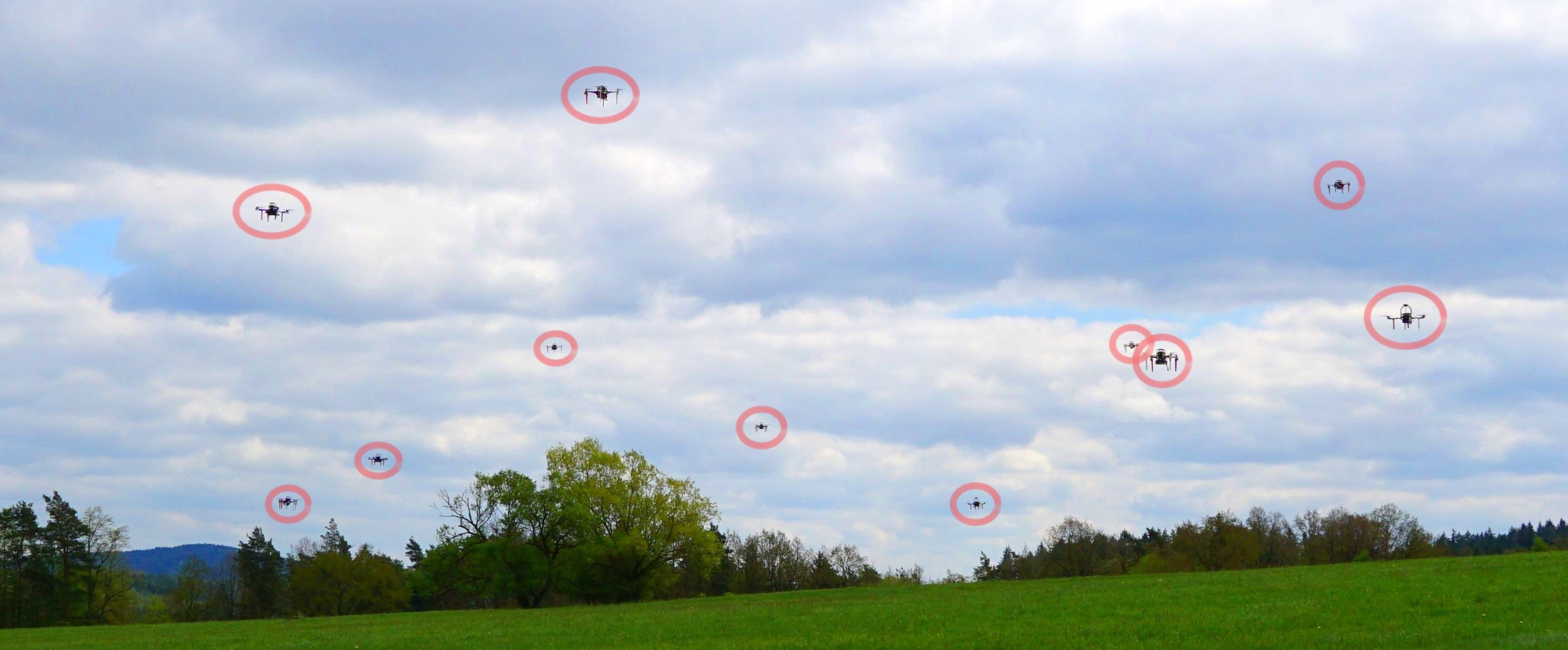
Figure 1: Experimental verification of the proposed approach in the field with $11$ UAVs.

In this paper, we propose a unified solution both for persistent monitoring (for all the robots) and target detection. In particular, we want to synthesize an algorithm that steers each robot to continuously span all the mission space, providing guarantees for target detection in finite time. In the literature, there are a few works that address this problem. In [12, 13] solutions based on Lissajous curves [26] are provided to solve the problem. In particular, the authors provide to the robots precomputed trajectories to follow through a tracking algorithm, however no information about the neighbors state is considered during the mission, making the solution not robust to synchronization errors.

In our previous work [8], we combined the Time-inverted Kuramoto dynamics [7] with Lissajous curves properties to obtain a distributed algorithm, which promotes robustness and resiliency during the mission. A coordination strategy based on guiding vector field and consensus is proposed in [30]. Nevertheless, it requires the desired distance between robots to be specified, hence it relies on the number of robots in the network to achieve the desired robot deployment. Moreover, the time-inverted Kuramoto model offers the possibility to reach also alternative equilibrium configurations autonomously, i.e., $\kappa$-cluster equilibrium points (see Section 2).

Another crucial lack in the literature is the absence of deployment and assessment of generic coverage algorithm on aerial robotic platforms in the field. In fact, all the mentioned works implement their algorithms only in simulated or controlled environments with very limited areas of interest. They typically assume an ideal localization system, and the actual implementation is often centralized. These scenarios lack disturbances and have negligible communication delays due to their relative simplicity. A quite limited amount of implementations on the field for multi-robot coverage algorithms can be found in the literature [1, 4, 28, 16]. However, all these approaches follow precomputed trajectories. In particular, there is no online coordination between robots during the mission. Hence, these algorithms are not robust nor resilient to uncertainties, failures or tracking errors, which may occur during the algorithm execution.

Finally, we cover the case where the robots experience unexpected events, e.g., malicious attacks, communication delays, tracking errors and other failures such as battery depletion or communication loss, which often occur during real-world deployment. Also this research line is quite unexplored [22, 31]. In our previous work [9], we provided sufficient conditions for stability and showed the degree of resiliency of the system to attacks and failures, without providing an effective solution to mitigate their effects. In [13], the authors proposed a method to reconfigure the formation that allows to add, remove and replace robots from the swarm. However, it needs all the robots in the network to be aware of the new parameter changes, which may introduce scalability issues.

Our contribution is threefold. Firstly, we designed a novel approach for aerial robots persistent monitoring and target detection in the three dimensional case, relying on the theoretical study we presented in [8] for ground robots. Notice that, with respect to existing methods for persistent monitoring and target detection [12, 13], our solution does not rely on precomputed trajectories, but it implements a constant feedback action on the basis of the neighbors state. Secondly, we show how the proposed approach can be adopted in case of short-time failures (type I), such as tracking errors, and long-time failures (type II), such as malicious attacks or battery depletion, providing a detailed analysis on the conditions to obtain persistent monitoring and target detection guarantees. Even by considering these additional challenges, we preserve the distributed nature of the approach, and its scalability. Finally, we bridge the gap between theory and practice by implementing the proposed algorithm in the field. In particular, we implement the approach on up to $11$ UAVs and analyzed the collected data, thereby validating the proposed method.

2 Problem description and proposed solution

In this section, we provide the problem description and the proposed solution that rely on our previous work [8]. Notice that with respect to [8], in this section, we proposed new findings related to the three dimensional case and properties required by the real-world deployment.

2.1 Problem description

The problem that we want to address reads as follows:

Problem 1. Given a rectangular space of interest of dimensions $[-A,A]\times[-B,B]$ and $N$ aerial robots with equal sensing range of radius $r_{s,i}=r_{s},\forall i=1,\dots,N$. We want to design a distributed control algorithm that satisfies the following requirements:

• The entire rectangular search area must be continuously monitored by the sensors of all the robots.

• Any element (stationary or moving) introduced into the mission area must be detected within a finite time.

• Robots must avoid collisions with each others.

• Robots must follow smooth paths.

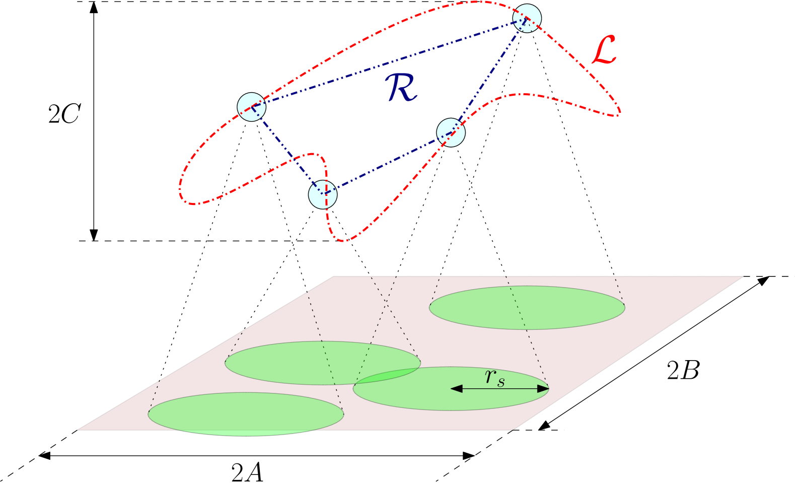
Figure 2: Problem illustration. The rectangular space of dimension $[-A,A]\times[-B,B]$ indicates the area of interest. Cyan circles indicate the robots’ positions, $\mathcal{L}$ indicates the path on which the robots are constrained to move, $\mathcal{R}$ describes the communication topology, and $r_{s}$ represents the sensing radius, equal for each robot.

To solve Problem 1, we considered the following assumptions.

Assumption 1 (Motion constraints).

Each robot is constrained to move along a closed path $\mathcal{L}\in\mathbb{R}^{3}$ ($\mathcal{L}\subset[-A,A]\times[-B,B]\times[-C,C]$), which can be represented in the parametric form $r(\gamma):\mathbb{R}\rightarrow\mathbb{R}^{3}$, $\gamma\in[0,2\pi)$. The $i$–th robot position in the three dimensional space is $r(\theta_{i})$, where $\theta_{i}\in\mathbb{R}$ identifies the state of the $i$–th robot.

Remark 1.

Notice that, due to the complex dynamics of aerial robots, tracking errors are unavoidable. An insight discussion on that can be found in the experimental results section.

Assumption 2 (Communication network).

Let us define the set $\mathcal{V}=\{1,\dots,N\}$, we denote by $\mathcal{V}(i)$ the $i$–th entry of $\mathcal{V}$. We consider to have a communication network topology that is an undirected ring $\mathcal{R}=\{(\mathcal{V}(i),j):j=\mathcal{V}(i+1),\forall i=1,\dots,N-1\}\cup\{(\mathcal{V}(i),j):j=$ $\mathcal{V}(i-1),\forall i=2,\dots,N\}\cup\{(\mathcal{V}(1),\mathcal{V}(N))\}\cup\{(\mathcal{V}(N),\mathcal{V}(1))\}$, where an arbitrary order of the $\mathcal{V}$ entries is allowed. In plain words, each robot communicates with exactly two robots and the overall graph is connected. Each robot can communicate its state $\theta_{i}$ to agent $j$ only if $j\in\mathcal{R}_{i}$, where $\mathcal{R}_{i}\subset\mathcal{R}$ indicates the neighbors of agent $i$.

Assumption 3 (Sensing range).

We assume that each robot has the same sensing radius $r_{s}$ and this value is constant. In practice this is not strictly true due to different altitude and/or terrain conditions. Nevertheless, since we consider relatively small variations in the $z$-axis, we can hold the assumption.

The introduced problem is illustrated in Figure 2.

2.2 Proposed solution

Our solution to Problem 1 relies on the combination of the time-inverted Kuramoto dynamics, which provides the coordination strategy, and the Lissajous curves, which provide the space where the robots move.

2.2.1 Time-inverted Kuramoto model

The time-inverted Kuramoto model is a variation of the classic Kuramoto model [21]. It can be written as follows

$$\dot{\theta}_{i}=\omega-K\sum_{j\in\mathcal{R}_{i}}\sin\left(\theta_{j}-\theta_{i}\right),\quad\forall i=1,\ldots,N,$$ (1)

where $\omega\in\mathbb{R}$ is the angular velocity, $K\in\mathbb{R}$ is a tuning parameter that weights the feedback action, and $\mathcal{R}_{i}\subset\mathcal{R}$ indicates the neighbors of agent $i$ defined in Assumption 2. In our previous works [7, 9, 8], we deeply analyzed the behavior of this nonlinear dynamical system. In the following, we recall some of the properties of interest for Problem $1$. Let us assume to observe the evolution of the states $\theta_{i}$ from a mobile reference frame, which rotates with a constant speed equal to $\omega$. Since $\omega$ is the same for all the robots, without loss of generality we can assume that $\omega=0$.

Theorem 1 (Convergence to the equilibrium [9]).

The dynamical system (1) converges to the equilibrium point

$$\begin{split}\theta^{\star(p)}=[\theta_{0}+2z_{1}\pi,\theta_{0}+2z_{2}\pi+\frac{2\pi p}{N},\ldots\\ \ldots,\theta_{0}+2z_{N}\pi+\frac{2\pi p(N-1)}{N}]^{\top},\end{split}$$ (2)

where $\theta_{0}\in\mathbb{R}$ can be any real number, $p\in\mathcal{P}_{k}=\{y\in\mathbb{Z}\mid y\in(N/4+kN,3N/4+kN),\forall k\in\mathbb{Z}\}$, and $z_{i}\in\mathbb{Z}$ for all $i=1,\dots,N$.

Definition 1 (Cluster [9]).

A set $\mathcal{Y}$ of robots forms a cluster if for every $i,j\in\mathcal{Y}$ there exists $k\in\mathbb{Z}$ such that $\theta_{i}-\theta_{j}=2k\pi$.

Lemma 1 ($\kappa$-clustered coverage [9]).

Given $N>2$ and the dynamics (1), the number of agents that cluster together at the stable equilibrium point (2) is given by the greatest common divisor between $N$ and $p$, denoted by $\kappa=$gcd$(N,p)$.

To resume, the dynamics (1) converges to well defined stable equilibrium points, namely $\kappa$-clustered equilibrium points.

2.2.2 Lissajous curves

When the equilibrium positions of the Time-inverted Kuramoto dynamics meet the Lissajous curves we obtain remarkable properties. Let us start by analyzing the two dimensional Lissajous curves

$$\begin{split}x(\gamma)=A\cos(a\gamma)&,\,\,y(\gamma)=B\sin(b\gamma),\end{split}$$ (3)

where $A,B\in\mathbb{R^{+}}$ are scalar values that define the area of interest, $a,b\in\mathbb{Z}^{+}$, co-prime and with $a$ as an odd number.

Definition 2 (Non-degenerate Lissajous curve).

It refers to a Lissajous curve in the parametric form (3), which traces a continuous multi-looped, and non-overlapping pattern in the interval $\gamma\in[0,2\pi)$. Notice that these curves may present points intersections, but not path overlapping routes (it is not doubly traversed). The conditions to have non-degenerate curve are $A,B\in\mathbb{R^{+}}$, $a,b\in\mathbb{Z}^{+}$, co-prime and with $a$ as an odd number.

By relying on the results in [12, 8] and by considering the equilibrium coordinates (2), for the $i$–th robot we have

$$\left(x_{i}(\gamma),y_{i}(\gamma)\right)=\left(A\cos(\theta_{i}^{\star(p)}-a\gamma),B\sin(\theta_{i}^{\star(p)}+b\gamma)\right).$$ (4)

By assuming $a+b=N/\kappa$, the robots lie on the curve

$$\frac{y^{2}}{B^{2}}+\frac{x^{2}}{A^{2}}-\frac{2xy\sin((a+b)\gamma)}{AB}=\cos^{2}((a+b)\gamma),$$ (5)

which defines a set of ellipses centered in the origin and inscribed in the mission space. Hence, we can state that by imposing (1) with $\omega\neq 0$, at the equilibrium (2), the following properties hold.

Property 1 (Complete coverage).

The condition on the sensing range of each robot that allows to cover all the mission space reads as

$$r_{s}>\max\left\{B\sin\left(\frac{\pi}{2a}\right),A\sin\left(\frac{\pi}{2b}\right)\right\}.$$ (6)

Property 2 (Target detection).

The condition on the sensing range for each robot that allows the fleet to detect arbitrary moving targets or events in a finite time reads as

$$r_{s}\geq\sin\left(\frac{\pi}{N/\kappa}\right)\sqrt{A^{2}+B^{2}}.$$ (7)

Hence, by exploiting the properties of the Time-inverted Kuramoto model and the Lissajous curves, we can obtain an effective strategy for both persistent monitoring (complete coverage) and target detection. Under these conditions we can also compute the maximum target detection time $T^{\max}_{\text{tar}}=\frac{2\pi/\omega}{N/\kappa}$, which correspond to the time for each robot to sweep $\Delta\theta=\frac{2\pi}{N/\kappa}$, hence to cover all the mission space.

Depending on the equilibrium of the system, we can solve the task by maximizing parallelization ($1$-clustered equilibrium) or promoting redundancies ($\kappa$-clustered equilibrium with $\kappa>1$). Nevertheless, in both cases, we need to take care of collision avoidance between robots.

By construction, it is shown in [12, 8] that at the 1-clustered equilibrium positions (1) there are no collisions among the robots under the condition

$$r^{\max}_{i}<\sin\left(\frac{\pi}{N}\right)\frac{AB}{\sqrt{A^{2}a^{2}+B^{2}b^{2}}}.$$ (8)

Where $r^{\max}_{i}$ indicates the maximum radius of encumbrance for the robots in the fleet. However, this condition is valid only at the (1-clustered) equilibrium and, since it is a sufficient condition, it is quite restrictive. This issue can be overcome in the following ways: i. by implementing a low level safety controller and ii. by means of three dimensional Lissajous curves.

In this work, we consider the 1-clustered equilibrium case, and we rely on a combination of the two solutions described above. In particular, a low level controller for collision avoidance that can operate only in the $z$-axis, to not affect the coverage performance of the algorithm, i.e., to not affect the robots’ motion in the x-y plane. Alongside, we rely on three dimensional Lissajous curves, which allows to notably increase the value of $r_{i}^{\max}$.

The three dimensional Lissajous curves can be written as

$$\begin{split}x(\gamma)=A\cos(a\gamma)&,\,\,y(\gamma)=B\sin(b\gamma),\\ z(\gamma)=C&\cos(c\gamma+\varphi).\end{split}$$ (9)

Similarly to the two dimensional case, we select $a,b,c\in\mathbb{Z}^{+}$, co-prime, with $a$ as an odd number. The latter condition ensures that the Lissajous curve is non-degenerate in the $x$-$y$ plane. In this way, we obtain a desired non-degenerate Lissajous curve that has the additional property of not having intersecting point. This curve is also called Lissajous knot [5]. More formally:

Lemma 2 (Lissajous knot).

Given the three dimensional Lissajous curve in (9), if $A,B,C\in\mathbb{R^{+}}$ and $a,b,c\in\mathbb{Z^{+}}$ are co-prime, then the curve is non-degenerative and without points of intersection, i.e., it is a Lissajous knot.

Proof.

The co-prime condition between $a,b$ and $c$, implies that all the points on the Lissajous curve given $\gamma\in[0,2\pi)$ are distinct. This can be verified by solving the following linear system in $\gamma_{1},\gamma_{2}$:

$$x(\gamma_{1})=x(\gamma_{2}),y(\gamma_{1})=y(\gamma_{2}),z(\gamma_{1})=z(\gamma_{2}),$$ (10)

by substituting (9) to (10), we can write:

$$\begin{cases}\gamma_{1}=\gamma_{2}+\frac{2\pi k_{1}}{a}\,\,\vee\,\,\gamma_{1}=-\gamma_{2}+\frac{2\pi k_{2}}{a}\\ \gamma_{1}=\gamma_{2}+\frac{2\pi k_{3}}{b}\,\,\vee\,\,\gamma_{1}=\frac{\pi}{b}-\gamma_{2}+\frac{2\pi k_{4}}{b}\\ \gamma_{1}=\gamma_{2}+\frac{2\pi k_{5}}{c}\,\,\vee\,\,\gamma_{1}=-\gamma_{2}-\frac{2\varphi}{c}+\frac{2\pi k_{6}}{c},\\ \end{cases}$$ (11)

where $k_{1,..,6}\in\mathbb{Z}$. It can be noticed, by solving the system of equations, that if $a,b,c$ are co-prime, for $\gamma_{1}\neq\gamma_{2}$ and $\gamma_{1},\gamma_{2}\in[0,2\pi)$, it does not have solutions. Hence the proof. ∎

The non-intersecting property serves a dual purpose: first, as we will show in the following section, it simplifies the robots’ initialization process, second, it is the main responsible of the increase in the safety distance. In fact, given a Lissajous curve in the $x$-$y$ plane, by adding a third dimension and ensuring to not have self-intersections, it implies an increase of the safety distance.

Remark 2.

The selection of the parameters $C,c,\varphi$ affects the safety distance $r_{i}^{\max}$. The analytical expression for the relation between $r_{i}^{\max}$ and $C,c,\varphi$ is not straight forward, hence the selection of the parameters can be done empirically or by numerically solving an optimization problem.

Remark 3 (3D Lissajous curve).

Notice that the three dimensional Lissajous curve can be used also to solve three dimensional coverage problems, e.g., structure coverage [23], and the time-inverted Kuramoto model can be applied also to these problems to coordinate multiple robots promoting parallelization and redundancies.

2.3 Numerical example

To show both scalability, and the advantages of 3D Lissajous curves and Time-Inverted Kuramoto model over [12], we run few simulations with different settings: 1. Algorithm [12] on 2D Lissajous curves, 2. Time-inverted Kuramoto algorithm on 3D Lissajous curves, 3. Algorithm [12] on 2D Lissajous curves with asynchronous start and 4. Time-inverted Kuramoto algorithm on 2D Lissajous curves with asynchronous start. To represent the synchronization issue, we start the system in a configuration which slightly deviates from the equilibrium. For all the simulations we used the following parameters $N=50$, $A=100$ (m), $B=100$ (m), $C=5$ (m) ($C=0$ (m) for the 2D case), $a=23$, $b=27$, $c=5$, $\omega=0.01$ (rad/s), $K=1000$, $dt=0.01$ (s). For all the cases we pick as metric the minimum distance between two robots in time, which is reported in Figure 3. As it can be noticed, 1. the use of 3D Lissajous curves allows to significantly increase the minimum distance between robots $d_{\min}$ and 2. The use of Time-inverted Kuramoto algorithm allows to quickly recover from the incorrect initial configuration, while [12] does not overcome this issue because does not use information about neighboring robots as feedback.

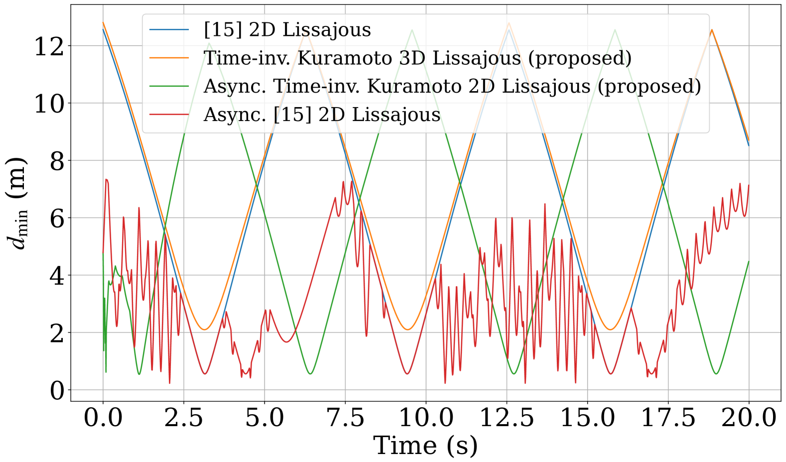
Figure 3: Minimum distance between robots in different configurations. In blue the results obtained by relying on  [12] and 2D Lissajous curves. In orange the Time-inverted Kuramoto algorithm on 3D Lissajous curves. In green the Time-inverted Kuramoto algorithm on 2D Lissajous curves with incorrect initial configuration. Finally in red, [12] with incorrect initial configuration on 2D Lissajous curves.

3 Deployment in real scenarios

In this section we discuss some practical aspects that has to be taken into account when the algorithm is deployed on a swarm of UAVs in the field. In the following, we discuss about the choice of the number of robots, how to initialize the experiments, how to effectively apply the time-inverted Kuramoto control law on the UAVs, and how to deal with unexpected events.

3.1 Number of UAVs

The first crucial decision is related to the number of robots to use. This proper number is influenced by several factors, including the dimensions of the sensing range and mission space, and whether target detection guarantees are needed or rather simple persistent monitoring is sufficient. If we require the moving target detection guarantees, relying on equation (7), we obtain

$$N>\frac{\pi\kappa}{\arcsin\left(\frac{r_{s}}{\sqrt{A^{2}+B^{2}}}\right)}.$$ (12)

While, if we require only persistent monitoring, the number of robots can be lower. In fact, given the sensing range $r_{s}$ and the dimensions $A,B$, by satisfying Property 1, we can choose the values of $a$ and $b$, obtaining a valid solution for persistent monitoring of all the mission space. The main advantage of having multiple robots is the parallelization, which is translated in less time required to complete the task and the redundancy that provides robustness and resiliency as we will discuss later in this section.

After the selection of the number of robots, a safety check (8) is necessary. If the condition is not met, we need to rely on three dimensional Lissajous curves and/or on a low level safety controller. For the low level collision avoidance any algorithm can be employed as long as it operates on the $z$-axis. On the other hand, for the selection of a proper three dimensional Lissajous curve, we need to select the values of $C,c,\varphi$, as discussed in Remark 2.

3.2 Robots initialization

Another issue to consider when the algorithm is deployed in the field, concerns the robots’ state initialization. Depending on the robots’ initial positions, the final equilibrium may change. One possible approach is to compute the desired stable equilibrium positions in advance and then steer the robots to the equilibria by means of an effective multi-robot collision avoidance algorithms, such as [10]. Once the robots reach a neighbourhood of the desired position, they need to localize themselves on the Lissajous curve, hence each robot computes its state $\theta_{i}$, which corresponds to $\operatorname*{arg\,min}_{\theta_{i}}\|p_{i}-\mathcal{L}(\theta_{i})\|$. Notice that it can be done without any ambiguity by considering the three dimensional case. In fact, in this scenario each value $\theta_{i}$ corresponds to a unique robot position (see Lemma 2). It does not hold for the two dimensional case, which requires to be initialized by $\theta$ values. Hence, after the convergence towards the desired location, the time-inverted Kuramoto model can be applied. Notice that, once the $i$–th robot computes its state $\theta_{i}$, we also need to constraint its dynamics in order to avoid sudden jumps in the state estimation, which can be induced by tracking errors or due to the presence of path intersections for the two dimensional case.

3.3 Dynamic constraints

In addition to the uncertainties of the environment, e.g., turbulences and wind gusts, each UAV is a non-trivial dynamical system that cannot be modeled as a single integrator. Hence, to control the robots we rely on [2]. In particular, through the time-inverted Kuramoto model (1), we synthesize the velocity $\dot{\theta}_{i}$. By integration, we obtain the next desired state $\theta_{i}^{D}$, hence $p_{i}^{D}=r(\theta_{i}^{D})$, which is given as reference input to the MPC. The MPC control error is defined as follows

$$e[k]=x_{m}[k]-x_{m}^{D}[k],\,\,\,\forall k\{1,\dots,n\},$$ (13)

where $x_{m}[k]=[x,\dot{x},\ddot{x},y,\dot{y},\ddot{y},z,\dot{z},\ddot{z}]^{\top}$ is the state vector at the sample $k$ of the prediction, $n$ indicates the length of the prediction horizon, while $x^{D}_{m}[k]=[x^{D},0,0,y^{D},0,0,z^{D},0,0]$. The optimization problem is a QP problem and it can be written as follows:

$$\begin{split}\operatorname*{\min\text{imize}}_{u[0:n]}\frac{1}{2}\sum_{k=0}^{n-1}\left(e[k]^{\top}Qe[k]\right)+e[n]^{\top}Se[n],\\ s.t.\,\,\,x_{m}[k]=A_{m}x_{m}[k-1]+B_{m}u[k],\,\,\,\forall k\in\{0,\dots n\},\\ x_{m}[k]\leq x_{\max},\,\,\,\forall k\in\{0,\dots n\},\\ x_{m}[k]\geq-x_{\max},\,\,\,\forall k\in\{0,\dots n\},\\ u[k]-u[k-1]\leq\dot{u}_{\max}dt,\,\,\,\forall k\in\{1,\dots n\},\\ u[k]-u[k-1]\geq-\dot{u}_{\max}dt,\,\,\,\forall k\in\{1,\dots,n\},\end{split}$$ (14)

where $x_{\max}$ and $u_{\max}$ are state and control input saturation limits, the matrices $A_{m}$ and $B_{m}$ define the model, while $Q,S$ are the state penalization error and the final state penalization error respectively.

4 Resiliency to unexpected events

As we have mentioned, our algorithm has a strong component of redundancy. This is translated in an abundant use of resources (large number of robots), but at the same time also in a high degree of robustness and resilience to unexpected events such as malicious attacks, communication delays, tracking errors, battery depletion or communication loss.

Based on our long term experience with real-world experiments with aerial robots, we recognize two types of possible failures or unexpected events; the short-time failures (type I) and long-time failures (type II). The former is managed by the algorithm as it is. In fact, because of its feedback component, even if the system deviates from the equilibrium configuration the feedback action attracts the system state back to the equilibrium.

Theorem 2 (Resiliency to type I failures [8]).

Given a stable equilibrium configuration $\theta^{\star(p)}$, by perturbing the $i$–th agent by $\delta\theta_{i}$, if

$$\cos(\theta_{i}^{\star(p)}-\theta_{j}^{\star(p)}+\delta\theta_{i})<0,\,\forall j\in\mathcal{R}_{i},$$ (15)

then the equilibrium point does not change.

This case is shown in the experimental results section, where communication delays and tracking errors are present throughout the duration of the mission. This type of failures, in general, can cause small deviations from the equilibrium, by assuming small tracking errors and small communication delays. A simple solution to preserve persistent monitoring and target detection, despite type I failures, is to account for a slightly larger sensing radius for each robot, which has to be defined on the basis of the maximum tracking error:

$$r_{s}\geq\eta\sin\left(\frac{\pi}{N/\kappa}\right)\sqrt{A^{2}+B^{2}},$$ (16)

where $\eta>1$ is a parameter that depends on the maximum tracking error. On the other hand, type II failures, e.g., communication loss, large communication delays, battery depletion and malicious attack, can seriously affect the behavior of the whole system. In the following, we provide a solution to account for these types of failures.

Firstly, we assume that each robot is able to detect its own failure as well as their neighbors’ failures. This is a reasonable assumption, since undesired motion behaviors, communication issues, and battery depletion are in general detectable and observable by the robot itself and its neighbors (see detail of the MRS UAV system [2] where such data can be obtained). Each robot has to measure its $\Delta\theta^{\star}_{ij}$ at the equilibrium, which can be estimated by measuring the value of $\Delta\theta_{ij}=\theta_{i}-\theta_{j}$ when the $\sum_{j\in\mathcal{R}_{i}}\sin(\theta_{i}-\theta_{j})\approx 0$. The failure detection can be triggered by properly selecting a threshold parameter $\varepsilon_{th}$. If a failure is detected on robot $j$, the $i$–th robot spoofs a virtual agent $j$ at the estimated equilibrium distance $\Delta\tilde{\theta}^{\star}_{ij}$, i.e., $\tilde{\theta}_{j}=\theta_{i}+\Delta\tilde{\theta}_{ij}^{\star}$. On the other hand, the $j$–th robot will reach a pre-designed area $p_{out}$, which lies out of the mission space (or it will just land). Once robot $j$ is ready to rejoin the group, it can do it by reaching back the equilibrium position, which can be inferred by knowing its neighbors’ states. Once it consistently communicates its expected state $\theta_{j}$, the neighbors can remove the spoofed agent and the algorithm can continue to work in its normal conditions. For the sake of clarity, we report the pseudo-code of the whole algorithm (see Algorithm 1).

By relying on this solution, the system continues to evolve maintaining the same equilibrium using $N-N_{a}$ robots, where $N_{a}$ is the number of robots affected by type II failures. While as far as $N_{a}\neq N$, persistent monitoring is preserved, the target detection guarantee requires two conditions to be satisfied. In particular we can state the following:

Proposition 3 (Failure-resilient target detection).

Given $N$ robots, by assuming a proper selection of the Lissajous $\mathcal{L}(\gamma)$ curve and a $1$-clustered equilibrium position $\theta^{\star}$, such that $\theta^{\star}_{i-1}-\theta^{\star}_{i}=\frac{2\pi}{N},\forall i=1,\dots,N-1$, under the condition that 1. each robot follows Algorithm 1, 2. the number of failures is equal or less than $\lfloor N/2\rfloor$ 3. for all $\theta_{i},\theta_{k}\in\theta^{a}$, mod($\|\theta_{i}-\theta_{k}\|,2\pi)<\pi$, and 4. $\varepsilon_{th}$ is selected such that it activates the type II failure when the Euclidean distance between two neighboring robots is $d_{ij}>2\eta r_{s,i}$. Then target detection guarantees are preserved.

Proof.

Given that the equilibrium $\theta^{\star}$ is a stable equilibrium (by relying on equilibrium manipulation in [9]), let us consider $N~\rightarrow~\infty$. In this case, the sensing range required to have detection is $r_{s,i}\geq 0$, according to (7), and we can visualize the robot positions as a continuous curve which is defined as (5). We can state that there exists a time instant $t^{*}$ where all the robots are aligned on one of the diagonals of the rectangular area of interest. At that time instant, the robots $i\in\{i_{0},i_{0}+\lfloor N/2\rfloor\}$, where $0\leq i_{0}\leq\lfloor N/2\rfloor$, are positioned at the vertices of the rectangular area of interest. While the robots are in the other diagonal configuration at the time instants $t\in t^{*}\pm\frac{\pi}{N\omega}$. Since by definition (5), the curve that describes the robots’ positions is an ellipse inscribed in the rectangular area of interest, which evolves continuously in time, then in the time interval $t\in(t^{*}-\frac{\pi}{N\omega},t^{*}+\frac{\pi}{N\omega})$, by considering only $i\in\{i_{0},\dots,i_{0}+\lfloor N/2\rfloor\}$ as active sensors, we have target detection guarantees. Let us define the set $\mathcal{P}_{t}(N)=\bigcup\limits_{i=i_{0}}^{\lfloor N/2\rfloor}\mathcal{B}(p_{i}(t),r_{s})$, where $p_{i}(t)$ indicates the robots’ positions at time $t$, and $\mathcal{B}(m,n)$ indicates the ball set centered in $m$ with radius $n$. By considering $N$ as a finite number, thanks to Property $2$, we have that $P_{t}(\infty)\subset P(N)$ and, more in general, that $P_{t}(N+1)\subset P_{t}(N)$, hence also in this case target detection and persistent monitoring are conserved. However, this is true at the equilibrium or by assuming a prompt detection of the type II failure, which depends on $\varepsilon_{th}$. Since around the equilibrium $\theta^{\star}$ as long as $d_{ij}<2\eta r_{s,i}$, target detection guarantees is not violated, by setting $\varepsilon_{th}$ to activate the type II failure when $d_{ij}\geq 2\eta r_{s,i}$ ensures a prompt type II failure detection. ∎

To further validate the theoretical findings, we provide additional simulation results. In the following we report the time to detect $n_{t}=1000$ targets randomly moving in the mission space. By using a total of $N=50$ robots and running multiple simulations with random initial conditions, we reported the obtained average time to detect all the targets in the mission space. By selecting $A=B=100$ (m), $a=23$, $b=27$, $r_{s,i}$ as in (16) with $\eta=1.05$, $\omega=0.06$ (rad/s) and $N_{a}=[0,4,25]$, we obtained an average detection time equal to $T_{\text{tar}}=[1.3,1.76,3.34]$ (s). As it was expected all the target are detected in a finite-time, the time to detect all the targets grows with $N_{a}$ and for $N_{a}=0,T_{\text{tar}}<T^{\max}_{\text{tar}}$ for all the simulations.

Algorithm 1 Failure-Resilient Algorithm

1:Select the desired Lissajous curve $\mathcal{L}(\gamma)$

2:Select the desired starting equilibrium position $\theta^{\star}_{i}$

3:Steer the robot $i$ to the equilibrium position $\mathcal{L}(\theta^{\star}_{i})$

4:Compute $\theta_{i}\leftarrow\arg\min\|p_{i}-\mathcal{L}(\theta_{i})\|$

5:$\dot{\theta}^{D}_{i}\leftarrow$ (1)

6:$\theta_{i}^{D}\leftarrow\theta_{i}+dt\,\dot{\theta}^{D}_{i}$

7:$[x^{D},y^{D},z^{D}]^{\top}\leftarrow\mathcal{L}(\theta_{i}^{D})$

8:$u_{i}\leftarrow$ (14) compute the control inputs

9:while FailureDetected(j) and $\|\theta_{j}-\theta_{i}+\Delta\theta_{ij}^{\star}\|>\varepsilon_{\text{th}}$ do

10:  $\tilde{\theta}_{j}\leftarrow\theta_{i}+\Delta\tilde{\theta}_{ij}^{\star}$

11:end while

12:while FailureDetected(i) do

13:  Steer robot $i$ to $p_{out}$

14:end while

15:if FailureRecovered(i) then

16:  if $\|\theta_{j}-\theta_{i}+\Delta\theta_{ij}^{\star}\|>\varepsilon_{\text{th}}$ then

17:   $\theta_{i}^{D}\leftarrow\theta_{j}+\Delta\tilde{\theta}^{\star}_{ij}$

18:  end if

19:  if $\|\theta_{j}-\theta_{i}+\Delta\theta_{ij}^{\star}\|\leq\varepsilon_{\text{th}}$  then

20:   goto 4.

21:  end if

22:end if

5 Experimental results

To validate the theoretical results, we implemented the algorithm on MRS platforms based on F450 and Holybro X500 frames [19, 20]. For the localization, each robot relies on GPS signal, while the positions of the neighboring robots are communicated through WiFi interface. We evaluated three scenarios in the field. Firstly, we considered $7$ and $11$ aerial robots subject to type I failures. Then we verified a case with $5$ aerial robots subject to type II failures. As is shown in this section, our algorithm proves to be resilient and robust to both failures of type I and II. For the first experiment we selected $N=7$, $A=20$ (m), $B=20$ (m), $C=2$ (m), $a=3$, $b=4$, $c=5$, $r_{s,i}$ as in (16) with $\eta=1.05$, $\omega=0.03$ (rad/s), $K=30$, $dt=0.01$ (s).

Due to tracking error, we experienced a maximum lateral error between the robots and the Lissajous curve in the x-y plane of $d_{il}\approx 1.3$ (m). In Figure 4, we report the distances between adjacent robots in the x-y plane. The robots largely satisfy the threshold for the minimum distance (8), and also they keep the formation, without exceeding the maximum distance $2r_{s,i}~\eqref{eq:eta}$ with $\eta=1.05$, required for target detection guarantees in finite-time.

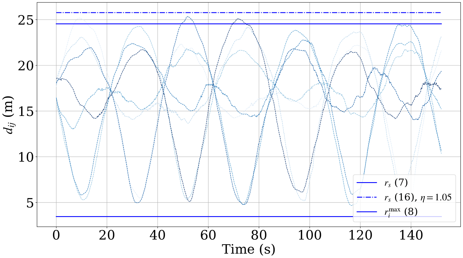
Figure 4: Experiment with $7$ UAVs. The dashed lines represent the distances between two adjacent robots $d_{ij}$ in the x-y plane in time. The solid lines are the theoretical lower and upper bounds for safety and target detection guarantees, respectively. The dashed dot line is two times the sensing radius adjusted by a factor $\eta=1.05$.

The correct behavior of the algorithm can be verified also from Figure 5, where we depict the values of $\theta_{i}$ for each robot as a function of time.

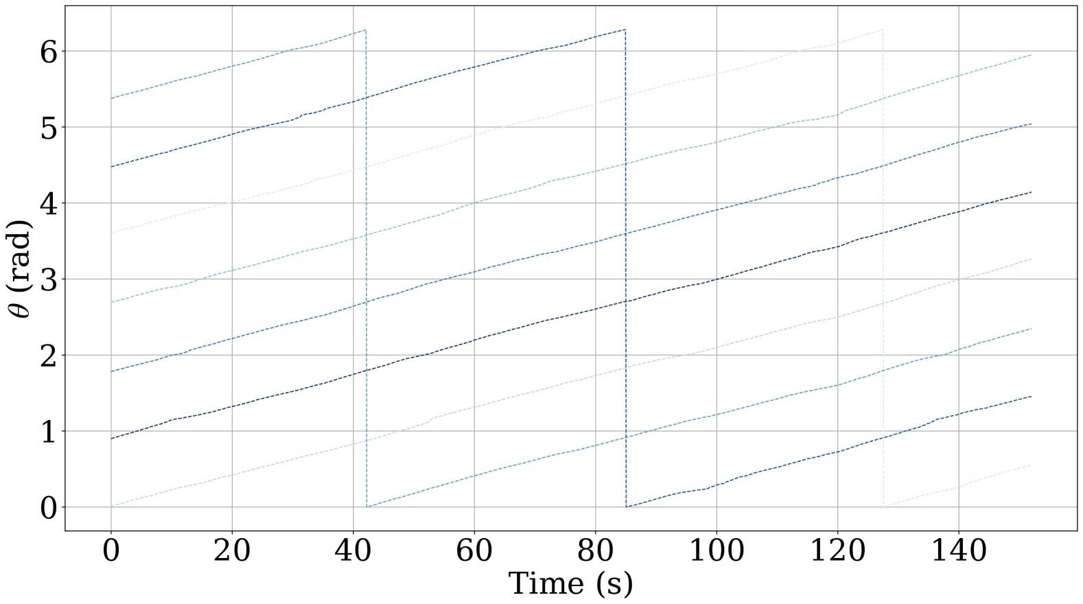
Figure 5: Experiment with $7$ UAVs. Values of the state $\theta_{i}$ for all the robots at each time step. Each color represents a different UAV for $i=1,\dots,7$.

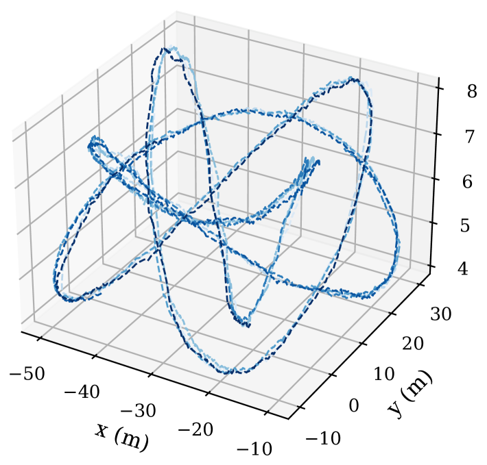
(a)	(b)

Figure 6: Experiment with $7$ UAVs. Path followed by the robots. In (a) the path from the top view, while in (b) the path seen from a different perspective to appreciate the displacements along the $z$-axis.

In Figure 6-(a) and in Figure 6-(b), we illustrate the paths followed by all the robots in the two and three dimensional spaces respectively. Finally, in Figure 7 we show the percentage of covered area with respect to time by accounting for a sensing range equal to $r_{s,i}$ (6). Also the complete coverage is achieved in accordance with the theoretical findings.

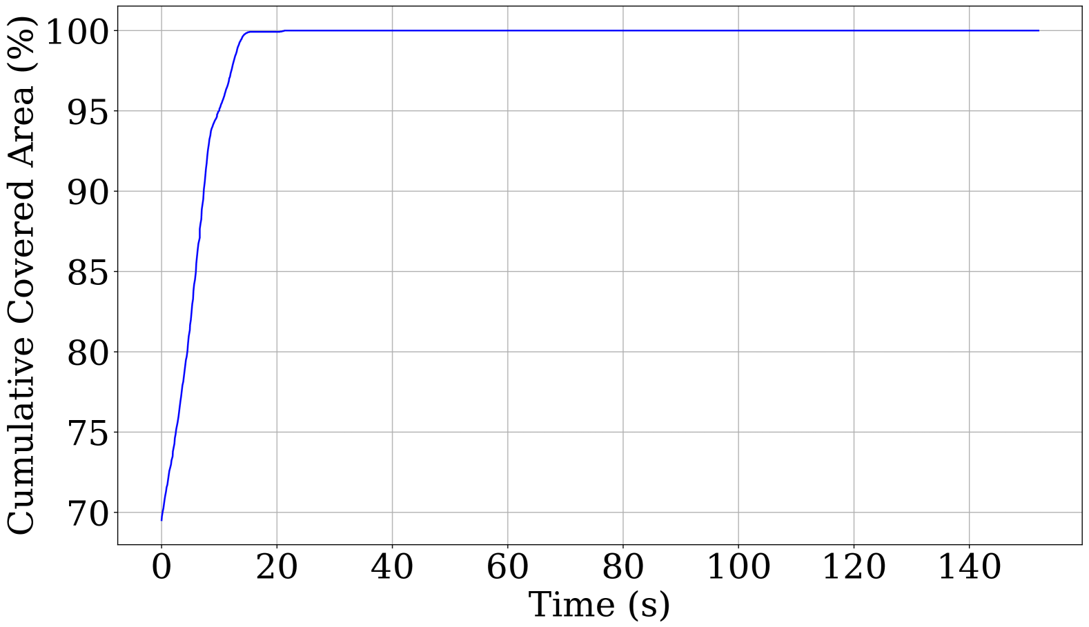
Figure 7: Experiment with $7$ UAVs. Percentage of the cumulative covered area with respect to time by accounting for a sensing range equal to $r_{s,i}$ (6).

In the second experiment, we consider the following parameters $N=11$, $A=20$ (m), $B=20$ (m), $C=3$ (m), $a=5$, $b=6$, $c=7$, $r_{s,i}$ as in (16) with $\eta=1.10$, $\omega=0.015$ (rad/s), $K=30$, $dt=0.01$ (s). Also in this case, we depict the same quantities obtaining similar results, confirming the scalability of the approach. In this case we obtained a maximum lateral error equal to $d_{il}\approx 1.2$ (m).

In Figure 8, we report the distances between adjacent robots in the x-y plane. Also in this case the safety distance is met. The maximum distance between adjacent robots to keep the guarantees of target detection, by considering $\eta=1.1$ in (16), is most of the time respected. In fact, some exceptions appear around $t=200$ (s), where the graph shows violations. The reason behind it, can be clearly inspected in Figure 9. Around the same time instant, it is possible to see that one robot stopped to move for a small amount of time. Due to large communication delays the robot did not update the positions of the neighbors and was stuck in the same position. After few seconds the robot received back the updated neighbors’ positions and the systems re-adapt and converge back to the correct equilibrium configuration. In practice these violations should be considered as type II failures (in accordance with Proposition 3), however to show the resiliency of the Time-inverted Kuramoto model we did not trigger Algorithm 1, nevertheless eventually the system get back to its correct equilibrium.

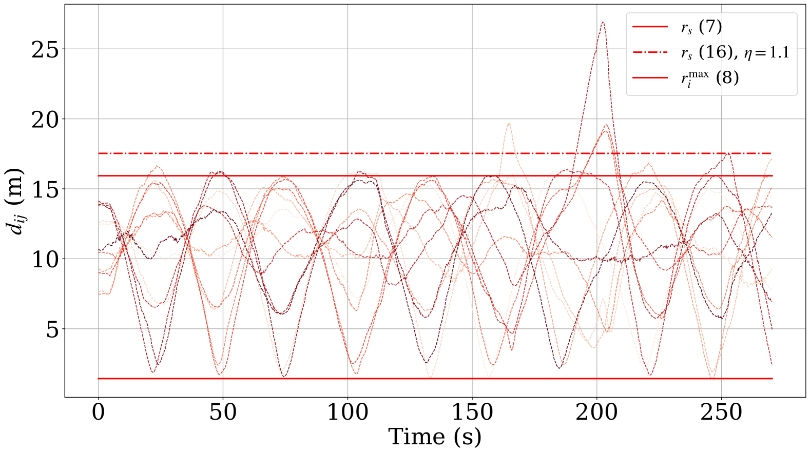
Figure 8: Experiment with $11$ UAVs. The dashed lines represent the distances in time from two adjacent robots $d_{ij}$ in the x-y plane. The solid lines are the theoretical lower and upper bounds for safety and target detection guarantees, respectively. The dashed dot line is two times the sensing radius adjusted by a factor $\eta=1.1$.

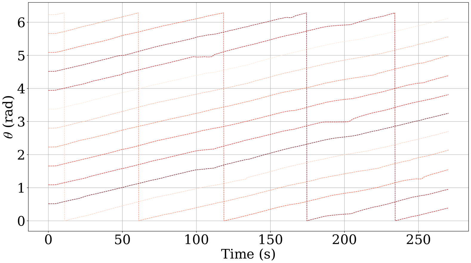
Figure 9: Experiment with $11$ UAVs. Values of the state $\theta_{i}$ for all the robots at each time step. Each color represents a different UAV for $i=1,\dots,11$.

In Figures 10-(a), 10-(b), we depict the paths followed by all the robots. Notice that the spikes in the z-axis are due to the low level safety controller that was engaged for safety reasons when two robots get too close to each other, notice that this behavior does not affect significantly the behavior in the x-y plane.

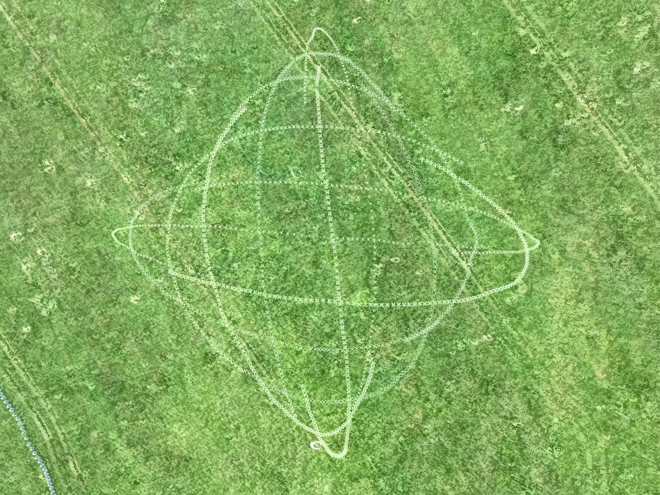
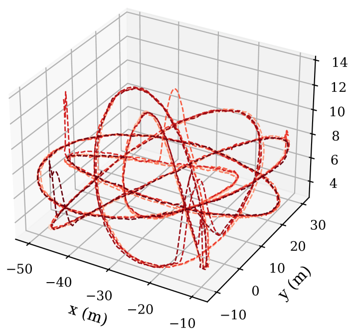
(a)	(b)

Figure 10: Experiment with $11$ UAVs. Path followed by the robots. In (a) the path from the top view, while in (b) the path seen from a different perspective to appreciate the displacements along the $z$-axis.

In Figure 11 we show the percentage of covered area with respect to time by accounting for a sensing range equal to $r_{s,i}$ (6). Also in this case the complete coverage is achieved in accordance with the theoretical findings.

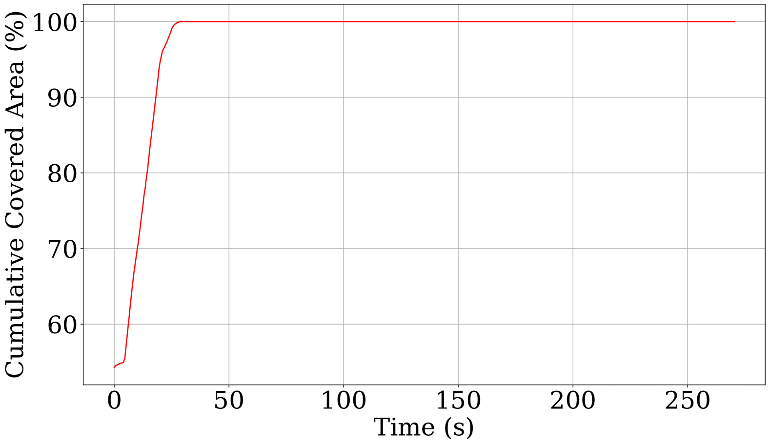
Figure 11: Experiment with $11$ UAVs. Percentage of the cumulative covered area with respect to time by accounting for a sensing range equal to $r_{s,i}$ (6).

Finally, in the third experiment, we considered the following parameters, $N=5$, $A=20$, $B=20$, $C=2$, $a=3$, $b=2$, $c=7$, $r_{s,i}$ as in (16) with $\eta=1.05$, $\omega=0.03$ (rad/s), $K=30$, $dt=0.01$ (s). We show the case where type II failures occur, and how the system reacts. In particular, we applied Algorithm $1$, by assuming that the robots’ failures are promptly detected by the neighbors.

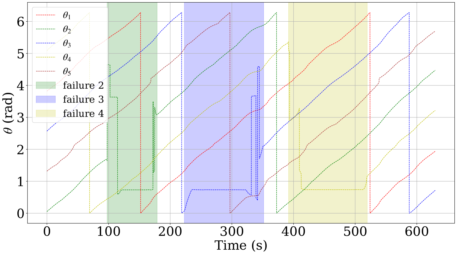
Figure 12: Experiment with $5$ UAVs. Values of the state $\theta_{i}$ for all the robots at each time step. The time interval of type II failure is highlighted in the plot.

In Figure 12, we depict the state of each robot $\theta_{i}$ for all $i=1,\dots,5$ and the phases where type II failure occurs. We show three consecutive failures on three different robots. The colored areas in the figure correspond to lines 11, 12 and 13, 14, 15 of the Algorithm 1. Also in this case, in Figure 13 we depict the distances $d_{ij}$ between two adjacent robots in the x-y plane. As it can be noticed, the algorithm proves to be resilient also to type II failures, and the experimental results are in line with the theoretical findings. In the multimedia materials we provide the videos of the experiments presented in this section.

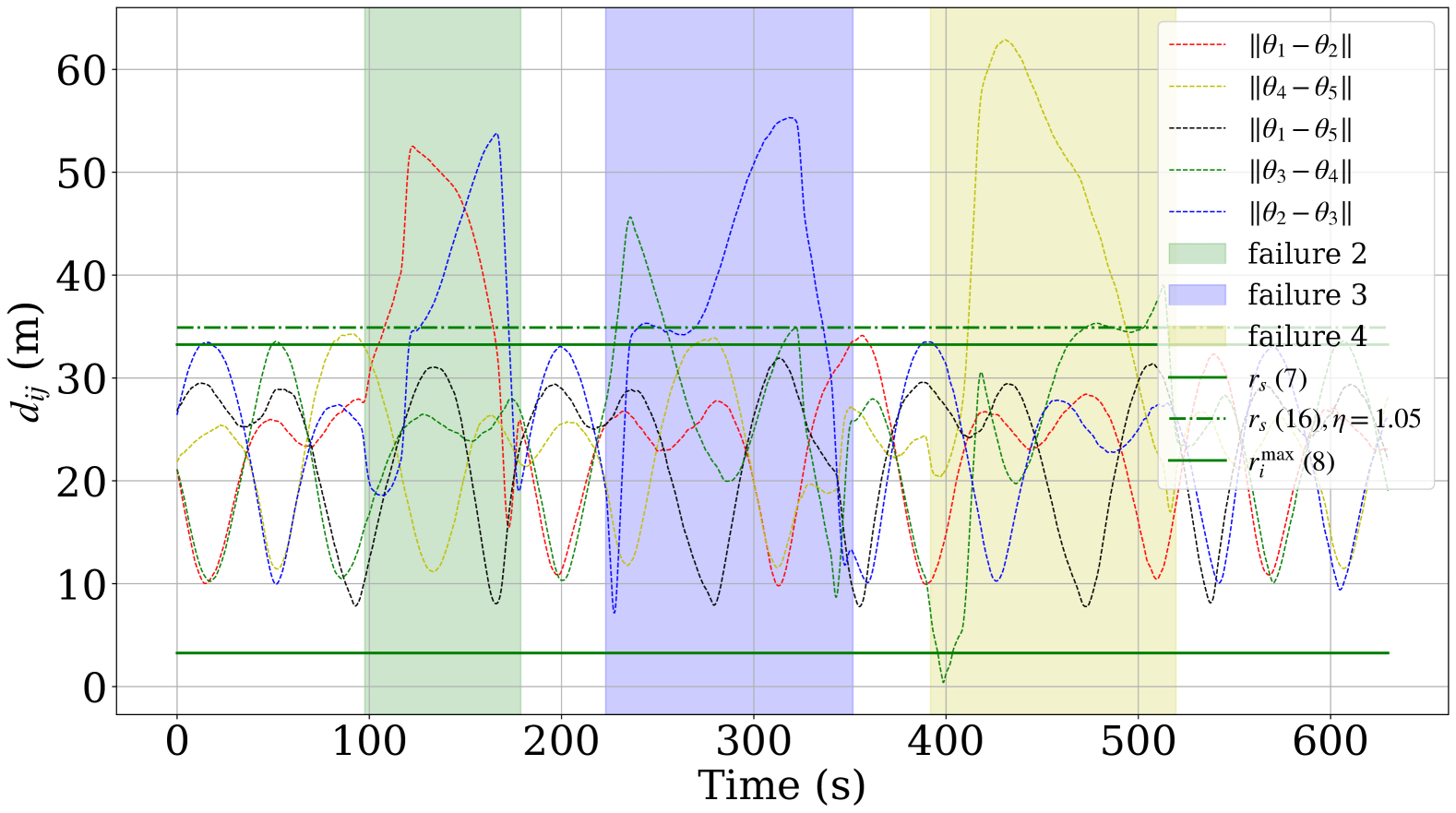
Figure 13: Experiment with $5$ UAVs. The dashed lines represent the distances in time from two adjacent robots $d_{ij}$ in the x-y plane. The solid lines are the theoretical lower and upper bounds for safety and target detection guarantees, respectively. The dashed dot line is two times the sensing radius adjusted by a factor $\eta=1.05$.

6 Conclusions

In this paper we presented a distributed control algorithm for multi-robot persistent monitoring and target detection. We provided a safe and effective solution for aerial robots in three dimensional spaces, which accounts for failures such as malicious attacks and/or batteries depletion. The algorithm has been largely tested in the field with up to eleven aerial robots. Future research directions will focus on the implementation of $\kappa$-clustered configurations, with $\kappa>1$, which needs alternative low-level controller for collision avoidance, on the implementation of the algorithm to solve three dimensional coverage problems for structural inspection (see Remark 3), on extensions to the case of non-rectangular mission space, and on an accurate evaluation on the algorithm energy efficiency.

References

- \bibcommenthead
- Apostolidis et al. [2022] Apostolidis SD, et al (2022) Cooperative multi-uav coverage mission planning platform for remote sensing applications. Autonomous Robots 46(2):373–400
- Baca et al. [2021] Baca T, et al (2021) The mrs uav system: Pushing the frontiers of reproducible research, real-world deployment, and education with autonomous unmanned aerial vehicles. Journal of Intelligent & Robotic Systems 102(1):26
- Bailon-Ruiz et al. [2022] Bailon-Ruiz R, Bit-Monnot A, Lacroix S (2022) Real-time wildfire monitoring with a fleet of uavs. Robotics and Autonomous Systems 152:104071
- Barrientos et al. [2011] Barrientos A, et al (2011) Aerial remote sensing in agriculture: A practical approach to area coverage and path planning for fleets of mini aerial robots. Journal of Field Robotics 28(5):667–689
- Bogle et al. [1994] Bogle M, Hearst J, Jones V, et al (1994) Lissajous knots. Journal of Knot Theory & Its Ramifications 3(2)
- Boldrer et al. [2019] Boldrer M, Fontanelli D, Palopoli L (2019) Coverage control and distributed consensus-based estimation for mobile sensing networks in complex environments. In: 2019 IEEE 58th Conference on Decision and Control (CDC), pp 7838–7843
- Boldrer et al. [2021] Boldrer M, Riz F, Pasqualetti F, et al (2021) Time-inverted kuramoto dynamics for -clustered circle coverage. In: 60th IEEE Conference on Decision and Control, pp 1205–1211
- Boldrer et al. [2022a] Boldrer M, Lyons L, Palopoli L, et al (2022a) Time-inverted kuramoto model meets lissajous curves: Multi-robot persistent monitoring and target detection. IEEE Robotics and Automation Letters 8(1):240–247
- Boldrer et al. [2022b] Boldrer M, Pasqualetti F, Palopoli L, et al (2022b) Multiagent persistent monitoring via time-inverted kuramoto dynamics. IEEE Control Systems Letters 6:2798–2803
- Boldrer et al. [2023] Boldrer M, et al (2023) Rule-based lloyd algorithm for multi-robot motion planning and control with safety and convergence guarantees. arXiv preprint arXiv:231019511
- Bolla et al. [2018] Bolla GM, et al (2018) Aria: Air pollutants monitoring using uavs. In: 5th IEEE Intern. Workshop on Metrology for AeroSpace, pp 225–229
- Borkar et al. [2016] Borkar A, Sinha A, Vachhani L, et al (2016) Collision-free trajectory planning on lissajous curves for repeated multi-agent coverage and target detection. In: 2016 IEEE/RSJ International Conference on Intelligent Robots and Systems (IROS), pp 1417–1422
- Borkar et al. [2020] Borkar AV, Hangal S, Arya H, et al (2020) Reconfigurable formations of quadrotors on lissajous curves for surveillance applications. European Journal of Control 56:274–288
- Carbone et al. [2022] Carbone C, et al (2022) Monitoring and mapping of crop fields with uav swarms based on information gain. In: Distributed Autonomous Robotic Systems: 15th International Symposium, Springer, pp 306–319
- Cortes et al. [2004] Cortes J, Martinez S, Karatas T, et al (2004) Coverage control for mobile sensing networks. IEEE Transactions on robotics and Automation 20(2):243–255
- Datsko et al. [2024] Datsko D, Nekovar F, Penicka R, et al (2024) Energy-aware multi-uav coverage mission planning with optimal speed of flight. IEEE Robotics and Automation Letters
- Durham et al. [2012] Durham JW, Franchi A, Bullo F (2012) Distributed pursuit-evasion without mapping or global localization via local frontiers. Autonomous Robots 32:81–95
- Franco et al. [2015] Franco C, et al (2015) Persistent coverage control for a team of agents with collision avoidance. Eur Journal of Control 22:30–45
- Hert et al. [2022] Hert D, et al (2022) Mrs modular uav hardware platforms for supporting research in real-world outdoor and indoor environments. In: International Conference on Unmanned Aircraft Systems, pp 1264–1273
- Hert et al. [2023] Hert D, et al (2023) Mrs drone: A modular platform for real-world deployment of aerial multi-robot systems. Journal of Intelligent & Robotic Systems 108(4):64
- Kuramoto and Kuramoto [1984] Kuramoto Y, Kuramoto Y (1984) Chemical turbulence. Springer
- Liu et al. [2021] Liu J, Zhou L, Tokekar P, et al (2021) Distributed resilient submodular action selection in adversarial environments. IEEE Robotics and Automation Letters 6(3):5832–5839
- Nath and Ghose [2024] Nath S, Ghose D (2024) Dynamic aerial coverage of stationary and moving structures using lissajous curves. In: AIAA SCITECH 2024 Forum, p 1991
- Pasqualetti et al. [2012] Pasqualetti F, Durham JW, Bullo F (2012) Cooperative patrolling via weighted tours: Performance analysis and distributed algorithms. IEEE Transactions on Robotics 28(5):1181–1188
- Pinto et al. [2020] Pinto SC, Andersson SB, Hendrickx JM, et al (2020) Optimal periodic multi-agent persistent monitoring of a finite set of targets with uncertain states. In: 2020 American Control Conference (ACC), pp 5207–5212
- Richards [1902] Richards HC (1902) On the harmonic curves known as lissa jous figures. Journal of the Franklin Institute 153(4):269–283
- Robin and Lacroix [2016] Robin C, Lacroix S (2016) Multi-robot target detection and tracking: taxonomy and survey. Autonomous Robots 40:729–760
- Shah et al. [2020] Shah K, Ballard G, Schmidt A, et al (2020) Multidrone aerial surveys of penguin colonies in antarctica. Science Robotics 5(47):eabc3000
- Smith et al. [2011] Smith SL, Schwager M, Rus D (2011) Persistent robotic tasks: Monitoring and sweeping in changing environments. IEEE Transactions on Robotics 28(2):410–426
- Yao et al. [2021] Yao W, de Marina HG, Sun Z, et al (2021) Distributed coordinated path following using guiding vector fields. In: IEEE International Conference on Robotics and Automation, pp 10030–10037
- Zhou and Kumar [2023] Zhou L, Kumar V (2023) Robust multi-robot active target tracking against sensing and communication attacks. IEEE Transactions on Robotics 39(3):1768–1780