Treewidth Parameterized by Feedback Vertex Number

Abstract

We provide the first algorithm for computing an optimal tree decomposition for a given graph $G$ that runs in single exponential time in the feedback vertex number of $G$, that is, in time $2^{\mathcal{O}(\mathsf{fvn}(G))}\cdot n^{\mathcal{O}(1)}$, where $\mathsf{fvn}(G)$ is the feedback vertex number of $G$ and $n$ is the number of vertices of $G$. On a classification level, this improves the previously known results by Chapelle et al. [Discrete Applied Mathematics ’17] and Fomin et al. [Algorithmica ’18], who independently showed that an optimal tree decomposition can be computed in single exponential time in the vertex cover number of $G$.

One of the biggest open problems in the area of parameterized complexity is whether we can compute an optimal tree decomposition in single exponential time in the treewidth of the input graph. The currently best known algorithm by Korhonen and Lokshtanov [STOC ’23] runs in $2^{\mathcal{O}(\mathsf{tw}(G)^{2})}\cdot n^{4}$ time, where $\mathsf{tw}(G)$ is the treewidth of $G$. Our algorithm improves upon this result on graphs $G$ where $\mathsf{fvn}(G)\in o(\mathsf{tw}(G)^{2})$. On a different note, since $\mathsf{fvn}(G)$ is an upper bound on $\mathsf{tw}(G)$, our algorithm can also be seen either as an important step towards a positive resolution of the above-mentioned open problem, or, if its answer is negative, then a mark of the tractability border of single exponential time algorithms for the computation of treewidth.

1 Introduction

Treewidth is (arguably) both the most important and the most well-studied structural parameter in algorithmic graph theory [11, 13, 15, 16, 17, 36, 43]. Widely regarded as one of the main success stories, most textbooks in parameterized complexity theory dedicate at least one whole chapter to this concept; see e.g. Niedermeier [50, Chapter 10], Flum and Grohe [35, Chapters 11 & 12], Downey and Fellows [34, Chapters 10–14], Cygan et al. [30, Chapter 7], and Fomin et al. [38, Chapter 14]. In particular, treewidth is a powerful tool that allows us to leverage the conspicuous observation that many NP-hard graph problems are polynomial-time solvable on trees. Here, many fundamental graph problems can be solved by simple greedy algorithms that operate from the leaves to the (arbitrarily chosen) root [27, 32, 39, 49]. Treewidth, intuitively speaking, measures how close a graph is to a tree. In slightly more formal terms, it quantifies the width of a so-called tree decomposition, which generalizes the property that trees can be broken up into several parts by removing single (non-leaf) vertices. Tree decompositions naturally provide a tree-like structure on which dynamic programming algorithms can operate in a straightforward bottom-up fashion, from the leaves to the root. The concept of treewidth has been proven to be extremely useful and has led to a plethora of algorithmic results, where NP-hard graph problems are shown to be efficiently solvable if we know a tree decomposition of small width for the input graph [2, 4, 5, 8, 10, 22]. Maybe the most impactful such result is Courcelle’s theorem [24, 28, 29], which states that all problems expressible in monadic second-order logic can be solved in linear time on graphs for which we know a tree decomposition of constant width.

In the early 1970s, Bertelè and Brioschi [9] first observed the above-described situation. They showed that a large class of graph problems can be efficiently solved by “non-serial” dynamic programming, as long as the input graph has a bounded dimension. Roughly 15 years later, this parameter was proven to be equivalent to treewidth [2, 14]. In the meantime, the concept of treewidth was rediscovered numerous times, for example by Halin [40] and, more prominently, by Robertson and Seymour [51, 52, 53] as an integral part of their graph minor theory, one of the most ground-breaking achievements in the field of discrete mathematics in recent history.

In order to perform dynamic programming on a certain structure, it is crucial that this structure is known to the algorithm. In the case of efficient algorithms for graphs with bounded treewidth, this means that the algorithm needs to have access to the tree decomposition. Since computing a tree decomposition of optimal width is NP-hard [3], many early works on such algorithms assumed that a tree decomposition (or an equivalent structure) is given as part of the input [2, 5, 8]. The first algorithm for computing a tree decomposition of width $k$ for an $n$-vertex graph (or deciding that no such tree decomposition exists) had a running time in $\mathcal{O}(n^{k+2})$ [3]. Shortly afterwards, an algorithm with a running time in $f(k)\cdot n^{2}$ was given by Robertson and Seymour [53]. It consists of two steps. In a first step, a tree decomposition of with at most $4k+3$ is computed in $O(3^{2k}\cdot n^{2})$ time (or concluded that the treewidth of the input graph is larger than $k$). In a second, non-constructive step (for which the function $f$ in the running time is not specified), this tree decomposition is improved to one with width at most $k$. In 1991, Bodlaender and Kloks [21], and Lagergren and Arnborg [47] independently discovered algorithms with a running time in $2^{\mathcal{O}(k^{3})}\cdot n$ for the second step. Furthermore, Bodlaender [12] gave an improved algorithm for the first step which allowed to compute a tree decomposition of width $k$ (or concluding that no such tree decomposition exists) in time $2^{\mathcal{O}(k^{3})}\cdot n$. These results have been extremely influential and allowed (among other things) Courcelle’s theorem [24, 28, 29] to be applicable without the prerequisite that a tree decomposition for the input graph is known. Roughly 30 years later, in 2023, Korhonen and Lokshtanov [46] presented an algorithm with a running time in $2^{\mathcal{O}(k^{2})}\cdot n^{4}$, which is considered a substantial break-through. Whether a tree decomposition of width $k$ (if one exists) can be computed in single exponential time in $k$, that is, a running time in $2^{\mathcal{O}(k)}\cdot n^{\mathcal{O}(1)}$, remains a major open question in parameterized complexity theory [46].

For many other graph problems, however, single exponential time algorithms in the treewidth of the input graph are known [5, 10, 18, 22, 31, 34, 35, 50]. If we want to use those algorithms to solve a graph problem, computing a tree decomposition of sufficiently small width becomes the bottleneck (in terms of the running time). Since we do not know how to compute a tree decomposition of minimum width in single exponential time, we have to rely on near-optimal tree decompositions if we do not want to significantly increase the running time of the overall computation. Therefore, much effort has been put into finding single exponential time algorithms that compute a tree decomposition with approximately minimum width, more specifically, with a width that is at most a constant factor away from the optimum. The first such algorithm was given by Robertson and Seymour [53] in 1995, and since then many improvements both in terms of running time and approximation factor have been made [1, 6, 7, 19, 45]. The current best algorithm by Korhonen [45] has an approximation factor of two and runs in $2^{\mathcal{O}(k)}\cdot n$ time. For an overview on the specific improvements, we refer to the paper by Korhonen [45].

Our Contribution. In this work, we focus on computing optimal tree decomposition. We overcome the difficulties of obtaining a single exponential time algorithm by moving to a larger parameter. The arguably most natural parameter that measures “tree-likeness” and is larger than treewidth is the feedback vertex number. It is the smallest number of vertices that need to be removed from a graph to turn it into a forest. Bodlaender, Jansen, and Kratsch [20] studied feedback vertex number in the context of kernelization algorithms for treewidth computation. The main result of our work is the following.

Theorem 1.1.

Given an $n$-vertex graph $G$ and an integer $k$, we can compute a tree decomposition for $G$ with width $k$, or decide that no such tree decomposition exists, in $2^{\mathcal{O}(\mathsf{fvn}(G))}\cdot n^{\mathcal{O}(1)}$ time. Here, $\mathsf{fvn}(G)$ is the feedback vertex number of graph $G$.

Theorem˜1.1 directly improves a previously known result, that an optimal tree decomposition for an $n$-vertex graph $G$ can be computed in $2^{\mathcal{O}(\mathsf{vcn}(G))}\cdot n^{\mathcal{O}(1)}$ time (if it exists) [26, 37], where $\mathsf{vcn}(G)$ is the vertex cover number of $G$, which is the smallest number of vertices that need to be removed from a graph to remove all of its edges, and hence always at least as large as the feedback vertex number. To the best of our knowledge, the only other known result for treewidth computation that uses a different parameter to obtain single exponential running time is by Fomin et al. [37], who showed that an optimal tree decomposition can be computed in $2^{\mathcal{O}(\mathsf{mw}(G))}\cdot n^{\mathcal{O}(1)}$, where $\mathsf{mw}(G)$ is the modular width of $G$. We remark that the modular width can be upper-bounded by a (non-linear) function of the vertex cover number, but is incomparable to both the treewidth and the feedback vertex number of a graph. It follows that our result improves the best-known algorithms for computing optimal tree decompositions (in terms of the exponential part of the running time) for graphs $G$ where

$$\mathsf{fvn}(G)\in o\bigl{(}\max\bigl{\{}\mathsf{tw}(G)^{2},\mathsf{vcn}(G),\mathsf{mw}(G)\bigr{\}}\bigr{)},$$

where $\mathsf{tw}(G)$ denotes the treewidth of $G$. On a different note, since $\mathsf{fvn}(G)$ is an upper bound on $\mathsf{tw}(G)$, our algorithm can also be seen either as an important step towards a positive resolution of the open problem of finding an $2^{\mathcal{O}(\mathsf{tw}(G))}\cdot n^{\mathcal{O}(1)}$ time algorithm for computing an optimal tree decomposition, or, if its answer is negative, then a mark of the tractability border of single exponential time algorithms for the computation of treewidth.

Our algorithm constitutes a significant extension of a dynamic programming algorithm by Chapelle et al. [26] for computing optimal tree decompositions which runs in $2^{\mathcal{O}(\mathsf{vcn}(G))}\cdot n^{\mathcal{O}(1)}$ time. The building blocks of the algorithm are fairly simple and easy to implement, however the analysis is quite technical and involved. First of all, our algorithm needs to have access to a minimum feedback vertex set, that is, a set of vertices of minimum cardinality, such that the removal of those vertices turns the graph into a forest. It is well-known that such a set can be computed in $2.7^{\mathsf{fvn}(G)}\cdot n^{\mathcal{O}(1)}$ time (randomized) [48] or in $3.6^{\mathsf{fvn}(G)}\cdot n^{\mathcal{O}(1)}$ deterministic time [44]. As a second step, we apply the kernelization algorithm by Bodlaender, Jansen, and Kratsch [20] to reduce the number of vertices in the input graph to $\mathcal{O}(\mathsf{fvn}(G)^{4})$. We remark that this kernelization algorithm needs a minimum feedback vertex set as part of the input and ensures that this set remains a feedback vertex set for the reduced instance [20]. This second step is neither necessary for the correctness of our algorithm nor to achieve the claimed running time bound, but it ensures that the polynomial part of our running time is bounded by the maximum of the running time of the kernelization algorithm and the polynomial part of the running time needed to compute a minimum feedback vertex set. Neither Bodlaender, Jansen, and Kratsch [20], Li and Nederlof [48], nor Kociumaka and Pilipczuk [44] specify the polynomial part of the running time of their respective algorithms. However, an inspection of the analysis for the kernelization algorithm suggests that its running time is in $\mathcal{O}(n^{5})$ and it is known that a minimum feedback vertex set can be computed in $2^{\mathcal{O}(\mathsf{fvn}(G))}\cdot n^{2}$ time [25].

In the following, we give a brief overview of the main ingredients of our algorithm. The main purpose of this overview is to convey an intuition and an idea of how the algorithm works; it is not meant to be completely precise.

• Chapelle et al. [26] introduced notions and terminology to formalize how a (rooted) tree decomposition interacts with a minimum vertex cover. We adapt and extend those notions for minimum feedback vertex sets. Inspired by the well-known concept of nice tree decompositions [21], we define a class of rooted tree decompositions that interact with a given feedback vertex set in a “nice” way. We call those tree decompositions $S$-nice, where $S$ denotes the feedback vertex set. In $S$-nice tree decompositions, we classify each node $t$ by which vertices of the feedback vertex set are contained in the bag and which are only contained in bags of nodes in the subtree rooted at $t$. We show that nodes of the same class form (non-overlapping) paths in the tree decomposition.

• We give algorithms to compute candidates of bags for the top and the bottom node of a path that corresponds to a given node class. Here, informally speaking, we differentiate between the cases where nodes (and their neighbors) have “full” bags or not, where we consider a bag to be full if adding another vertex to it increases the width of the tree decomposition. We need two novel algorithmic approaches for the two cases.

• We give an algorithm to compute the maximum width of any bag “inside” a path that corresponds to a given node class. This algorithm needs as input the bag of the top node and the bottom node of the path, and the set of vertices that should be contained in some bags of the path.

• The above-described algorithm allows us to perform dynamic programming on the node classes. Informally, we show that node classes form a partially ordered set. This means that for a given node class, we can look up a partial tree decomposition where the root belongs to a preceding (according to the poset) node class in a dynamic programming table. Then we use the above-described algorithm to extend the looked-up tree decomposition to one where the root has the given node class.

We show that in the above-described way, we can find a tree decomposition of width $k$ whenever one exists. To this end, we introduce (additional) novel classes of tree decompositions that have properties that we can exploit algorithmically. We introduce so-called slim tree decompositions, which, informally speaking, have a minimum number of full nodes and some additional properties. Furthermore, we introduce top-heavy tree decompositions, where, informally speaking, vertices are pushed into bags that are as close to the root as possible. We show that there exists tree decompositions with minimum width that are $S$-nice, slim, and top-heavy. Lastly, we give a number of ways to modify tree decompositions. We will show that we can modify any optimal tree decomposition that is $S$-nice, slim, and top-heavy into one that our algorithm is able to find.

Due to space constraints, we defer considerable amounts of technical details to a full version of this work. In Section˜2 we give an overview of the main parts of the algorithm. Afterwards, we introduce the most important concepts in and give some details on how the dynamic programming table looks like. The correctness proof and the running time analysis is deferred to the full version. Moreover, the full version contains expanded related work and additional illustrations.

2 Algorithm Overview

In this section, we take a closer look at the different building blocks of our algorithm before we explain each one in full detail. The goal of this section is to provide an intuition about how the algorithm works, that is fairly close to the technical details but not completely precise. We describe the main ideas of each part of the algorithm and how they interact with each other.

How Feedback Vertex Sets Interact With Tree Decompositions. Given a rooted tree decomposition $\mathcal{T}=(T,\{X_{t}\}_{t\in V(T)})$ of a graph $G$ and a minimum feedback vertex set $S$ for $G$, the feedback vertex set interacts with the bags of $\mathcal{T}$ is a very specific way. Given a bag $X_{t}$ of some node in $t$, we use $X_{t}^{S}=X_{t}\cap S$ to denote the vertices from $S$ that are inside the bag $X_{t}$. We use $L^{S}_{t}\subseteq S$ to denote the set of vertices from $S$ that are only in bags $X_{t^{\prime}}$ “below” $X_{t}$. More formally, bags $X_{t^{\prime}}$ of nodes $t^{\prime}$ that are descendants of node $t$. We use $R^{S}_{t}=S\setminus(L^{S}_{t}\cup X^{S}_{t})$ to denote the set of vertices in $S$ that are only in bags of nodes that are outside the subtree of $\mathcal{T}$ rooted at $t$. These three sets build a so-called $S$-trace, a concept introduced by Chapelle et al. [26]. One can show that the nodes in a tree decomposition that share the same $S$-trace partition the tree decomposition into path segments [26]. These path segments (or the corresponding $S$-traces) form a partially ordered set which, informally speaking, allows us to design a bottom-up dynamic programming algorithm that constructs a rooted tree decomposition for $G$ from the leaves to the root.

A similar approach was used by Chapelle et al. [26] to obtain a dynamic programming algorithm that has single exponential running time in the vertex cover number of the input graph. They use a minimum vertex cover instead of a minimum feedback vertex set to define $S$-traces. We extend this idea to work for feedback vertex sets, which requires a significant extension of almost all parts of the algorithm.

The main idea of the overall algorithm is the following. We give a polynomial-time algorithm to compute a partial rooted tree decomposition containing nodes corresponding to a directed path of an $S$-trace and, informally speaking, some additional nodes that only cover vertices from the forest $G-S$. We combine this partial rooted tree decomposition with one for the preceding directed paths according to the above-mentioned partial order. In other words, intuitively, we give a subroutine to compute partial tree decompositions for directed paths corresponding to $S$-traces, and try to assemble them to a rooted tree decomposition for the whole graph. We start with the directed paths that do not have any predecessor paths and then try to extend them until we cover all vertices. We save the partial progress we made in a dynamic programming table. The overall algorithm is composed out of fairly simple subroutines, which makes the algorithm easy to implement. However, a very sophisticated analysis is necessary to prove its correctness and the desired running time bound.

In order to bound the number of dynamic programming table look-ups that we need to compute a new entry, we need to be able to assume that the rooted tree decomposition we are aiming to compute behaves nicely (in a very similar sense as in the well-known concept of nice tree decompositions [21]) with respect to the vertices in $S$. To this end, we introduce the concept of $S$-nice tree decompositions and we prove that every graph $G$ admits an $S$-nice tree decomposition with minimum width for every choice of $S$.

Computing a “Local Tree Decomposition” for a Directed Path. The main technical difficulty is to compute the part of the rooted tree decomposition that contains the nodes corresponding to a directed path of an $S$-trace. As described before, these parts are the main building blocks with which we assemble our tree decomposition for the whole graph.

Our approach here is to compute candidates for the bags of the top node and the bottom node of the directed path corresponding to an $S$-trace. Intuitively, since the $S$-trace specifies where in the tree decomposition the other vertices from $S$ are located and since we know that $G-S$ is a forest, we have some knowledge on how these bags need to look like. If the bag $X$ we are computing is for a node that, when removed, splits the tree decomposition into few parts, then we can “guess” which vertices of $S$ are located in which of the different parts in an optimal tree decomposition. To this end, we adapt the concept of “introduce nodes”, “forget nodes”, and “join nodes” for $S$-nice tree decompositions. A consequence is that if a node does not share its bag $X$ with any neighboring node, then, when the node is removed, the tree decomposition splits into at most three relevant parts (that is, parts that contain bags with vertices from $S$ that are not in $X$). In other word, the bag $X$ acts as a separator for at most three parts of $S$. This allows us to compute a candidate for $X$ in a greedy fashion, and argue that we can modify an optimal tree decomposition to agree with our choice for $X$. An important property that we need for this is, that neighboring bags are not “full”, that is, their size is not $\mathsf{tw}(G)+1$, which gives us flexibility to shuffle around vertices.

However, if the optimal tree decomposition contains a large subtree of nodes that all have the same bag and that are all full, then removing those nodes can split the tree decomposition into an unbounded number of parts that each can contain a different subset of $S$. Here, informally speaking, we cannot afford to “guess” anymore how the vertices of $S$ are distributed among the parts and we cannot shuffle around vertices. Hence, we have to find a way to compute a candidate bag for this case where we do not have to change the tree decomposition to agree with our choice.

To resolve this issue, we need to refine the concept of $S$-nice tree decompositions. We introduce the slim $S$-nice tree decompositions that, informally speaking, ensure subtrees of the tree decomposition where all nodes have the same full bag have certain desirable properties that allow us to compute candidate bags efficiently. We prove that there are slim $S$-nice tree decomposition of minimal width for all graphs and all choices of $S$. Furthermore, we prove (implicitly) that we can bound the size of the search-space for a potential bag by a function that is single exponential in the feedback vertex number. Therefore, we will able to provide small “advice strings”, that lead our algorithm for this case to a candidate bag and we can prove that there is an advice string that will lead the algorithm to the correct bag.

Coordinating Between Different Directed Paths. Since we need to modify the optimal tree decomposition in order to agree with the bags that we compute, we have to make sure that later modifications do not invalidate earlier choices for bags. To ensure this, we introduce so-called top-heavy slim $S$-nice tree decompositions. Informally speaking, we try to push all vertices that are not in $S$ into bags as close to the root as possible. Intuitively, this ensures that if we make modifications to those tree decompositions to make them agree with our bag choices, those modifications do not affect bags that are sufficiently far “below” the parts of the tree decomposition that we modify.

Now, having access to the bag of the top node and the bottom node of a directed path corresponding to some $S$-trace, we have to decide which other vertices (that are not in $S$) we wish to put into bags that are attached to that path. Here, we also have to make sure that our decisions are consistent. We will compute a three-partition of the complete vertex set: one part that represents the vertices that are contained in some bag of the directed path or a bag that is attached to it, one part of vertice that are only in bags “below” the directed path, and the last part with the remaining vertices, that is, the vertices that are only in bags outside of the subtree of the tree decomposition that is rooted at the top node of the directed path. The first described part is needed to compute the partial tree decomposition of the directed path. We provide a polynomial-time algorithm to do this. Furthermore, the three-partition will allow us to decide which choices for bags to the top and bottom nodes of preceding directed paths are compatible with each other.

3 Main Concepts for the Algorithm

We use standard notation and terminology from graph theory [33]. A tree decomposition of a graph $G=(V,E)$ is a pair $\mathcal{T}=(T,\{X_{t}\}_{t\in V(T)})$ consisting of a tree $T$ and a family of bags $\{X_{t}\}_{t\in V(T)}$ with $X_{t}\subseteq V$, such that:

1. $\bigcup_{t\in V(T)}X_{t}=V$.

2. For every $\{u,v\}\in E$, there is a node $t\in V(T)$ such that $\{u,v\}\subseteq X_{t}$.

3. For every $v\in V$, the set $X^{-1}(v)=\{t\in V(T)\mid v\in X_{t}\}$ induces a subtree of $T$.

The width of a tree decomposition $\mathcal{T}=(T,\{X_{t}\}_{t\in V(T)})$ is $\max_{t\in V(T)}|X_{t}|-1$. The treewidth $\mathsf{tw}(G)$ of a graph $G$ is the minimum width over all tree decomposition of $G$.

We present several concepts introduced by Chapelle et al. [26] that we also use for our algorithm in Section˜3. In particular, we give the definitions of traces, directed paths thereof [26], and several additional concepts. The rest of the concepts (most of which are deferred to the full version) are novel. We introduce $S$-nice tree decompositions, which interact with a vertex set $S$ in a “nice” way, but are more flexible with vertices not in $S$. Finally, we introduce slim $S$-nice tree decompositions. This type of tree decompositions has crucial additional properties that we need to show that our algorithm is correct.

$S$-Traces, Directed Paths, $S$-Children, and $S$-Parents. Let $t$ be a node of a rooted tree decomposition $\mathcal{T}=(T,\{X_{t}\}_{t\in V(T)})$ of a graph $G=(V,E)$. We denote with $T_{t}$ the subtree of $T$ rooted at node $t$. We use the following notation throughout the document:

• The set $V_{t}=\bigcup_{t^{\prime}\in V(T_{t})}X_{t^{\prime}}$ is the union of all bags in the subtree $T_{t}$.

• The set $L_{t}=V_{t}\setminus X_{t}$ is the set of vertices “below” node $t$.

• The set $R_{t}=V\setminus V_{t}$ is the set of the “remaining” vertices, that is, the ones that are neither in the bag of node $t$ nor below $t$.

Clearly, for every node $t$, the sets $L_{t},X_{t},R_{t}$ are a partition of $V$.

Definition 3.1 ([26]) ($S$-Trace).

Let $G=(V,E)$ be a graph and tet $S\subseteq V$. Let $t$ be a node of a rooted tree decomposition $\mathcal{T}=(T,\{X_{t}\}_{t\in V(T)})$ of $G$. The $S$-trace of $t$ is the triple $(L_{t}^{S},X_{t}^{S},R_{t}^{S})$ such that $L_{t}^{S}=L_{t}\cap S$, $X_{t}^{S}=X_{t}\cap S$, and $R_{t}^{S}=R_{t}\cap S$. A triple $(L^{S},X^{S},R^{S})$ is an $S$-trace if it is the $S$-trace of some node in some tree decomposition of $G$.

Chapelle et al. [26] show that the nodes of a rooted tree decomposition that have the same $S$-trace form a directed path. They prove this for $S$-traces where $S$ is a minimum vertex cover and the rooted tree decomposition is nice, however inspecting their proof reveals that this property also holds for arbitrary sets $S$ and arbitrary rooted tree decompositions. Formally, we have the following.

Lemma 3.2 ([26]).

Let $\mathcal{T}=(T,\{X_{t}\}_{t\in V(T)})$ be a rooted tree decomposition of a graph $G=(V,E)$. Let $S\subseteq V$ and let $(L^{S},X^{S},R^{S})$ be an $S$-trace such that $L^{S}\neq\emptyset$. Moreover, let $N$ be the set of nodes of $\mathcal{T}$ whose $S$-trace is $(L^{S},X^{S},R^{S})$. Then the subgraph of $T$ induced by $N$ is a directed path.

Lemma˜3.2 allows us to define so-called directed paths of $S$-traces, which will be central to our algorithm. Informally, given an $S$-trace our algorithm will compute candidates for the corresponding directed path, and then use a dynamic programming approach to connect the path to the rest of a partially computed rooted tree decomposition.

Definition 3.3 (Directed Path of an $S$-Trace, Top Node, and Bottom Node).

Let $\mathcal{T}=(T,\{X_{t}\}_{t\in V(T)})$ be a rooted tree decomposition of a graph $G=(V,E)$, $S\subseteq V$ and $(L^{S},X^{S},R^{S})$ an $S$-trace such that $L^{S}\neq\emptyset$. We call the directed path induced by the set of nodes of $\mathcal{T}$ whose $S$-trace is $(L^{S},X^{S},R^{S})$ the directed path of $(L^{S},X^{S},R^{S})$ in $\mathcal{T}$ from node $t_{\max}$ to node $t_{\min}$. We call $t_{\max}$ the top node of the directed path and we call $t_{\min}$ the bottom node of the directed path.

We use the above concepts and some additional ones that we introduce below to define a specific type of rooted tree decomposition that interacts with the set $S$ in a very structured way. The concepts are illustrated in Figure˜1. First, we distinguish nodes that are at the end of a directed path of some $S$-trace.

Definition 3.4 ($S$-Bottom Node).

Let $\mathcal{T}=(T,\{X_{t}\}_{t\in V(T)})$ be a rooted tree decomposition of a graph $G=(V,E)$ and $S\subseteq V$. Let $t$ be a node of $\mathcal{T}$. We say that $t$ is an $S$-bottom node if there is an $S$-trace $(L^{S},X^{S},R^{S})$ such that $L^{S}\neq\emptyset$, and $t$ is the bottom node $t_{\min}$ of the directed path of $(L^{S},X^{S},R^{S})$ in $\mathcal{T}$.

Next, we observe that for every directed path of some $S$-trace, the parent of $t_{\max}$ is also an $S$-bottom node. Note that this implies that a situation as depicted in Figure˜1(b) cannot happen.

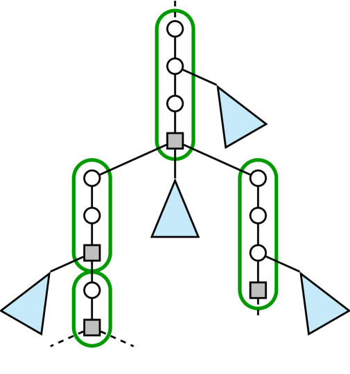
(a) Illustration of an $S$-nice tree decomposition.

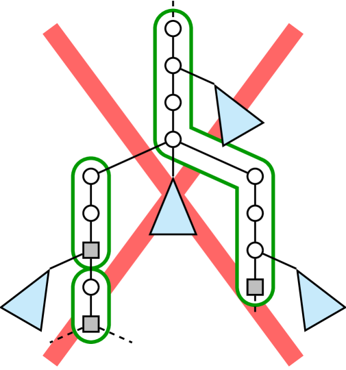
(b) This cannot happen.

Figure 1: Illustrations for the concepts of $S$-traces (Definition˜3.1) and their directed paths (Definition˜3.3), $S$-bottom nodes (Definition˜3.4), and $S$-nice tree decompositions (Definition˜3.6). The directed paths of different $S$-traces are surrounded by green lines. The $S$-bottom nodes are depicted as gray squares. The blue triangles illustrate parts of the tree decompositions where all nodes have $S$-traces with $L^{S}=\emptyset$, and hence are not part of any directed paths of $S$-traces. Subfigure 1(b) shows a configuration of directed paths of different $S$-traces that we can rule out.

We now define so-called $S$-parent and $S$-children. Informally, as $S$-child is a child of a node such that there is a vertex in $S$ that is only contained in nodes in the subtree of the tree decomposition rooted at the $S$-child. The $S$-parent of a node is defined analogously. Formally, we define them as follows.

Definition 3.5 ($S$-Parent and $S$-Child).

Let $\mathcal{T}=(T,\{X_{t}\}_{t\in V(T)})$ be a rooted tree decomposition of a graph $G=(V,E)$ and $S\subseteq V$. Let $t$ and $t^{\prime}$ be two nodes of $\mathcal{T}$ such that $t$ is the parent of $t^{\prime}$ in $T$. Let $(L_{t}^{S},X_{t}^{S},R_{t}^{S})$ and $(L_{t^{\prime}}^{S},X_{t^{\prime}}^{S},R_{t^{\prime}}^{S})$ be the $S$-traces of $t$ and $t^{\prime}$, respectively.

• If $(R_{t}^{S}\cup X_{t}^{S})\setminus(L_{t^{\prime}}^{S}\cup X_{t^{\prime}}^{S})\neq\emptyset$, then we say $t$ is an $S$-parent of $t^{\prime}$.

• If $(L_{t^{\prime}}^{S}\cup X_{t^{\prime}}^{S})\setminus(R_{t}^{S}\cup X_{t}^{S})\neq\emptyset$, then we say $t^{\prime}$ is an $S$-child of $t$.

$S$-Nice Tree Decompositions. We now give the definition of a so-called $S$-nice tree decomposition. Intuitively, this tree decomposition behaves nicely (in the sense of nice tree decompositions [21]) when interacting with vertices from the vertex set $S$, but is more flexible for the vertices in $V\setminus S$. Similarly to nice tree decomposition, $S$-nice tree decompositions distinguish three main types of $S$-bottom nodes, analogous to introduce, forget, and join nodes. We associate each $S$-bottom node with $S$-trace $(L^{S},X^{S},R^{S})$ with a so-called S-operation, which can be $\mathsf{introduce}(v)$ for some $v\in X^{S}$, $\mathsf{forget}(v)$ for some $v\in S\setminus X^{S}$, or $\mathsf{join}(X^{S},X_{1}^{S},X_{2}^{S},L_{1}^{S},L_{2}^{S})$ for some $X_{1}^{S},X_{2}^{S}\subseteq X^{S}$ and $L_{1}^{S},L_{2}^{S}\subseteq L^{S}$.

Definition 3.6 ($S$-Nice Tree Decomposition and $S$-Operations).

A rooted tree decomposition $\mathcal{T}=(T,\{X_{t}\}_{t\in V(T)})$ of a graph $G=(V,E)$ is $S$-nice for $S\subseteq V$ if the following hold. Let $t$ be a node. Then the following holds.

1. If $t$ has a parent $t^{\prime}$, then $X_{t}\subseteq X_{t^{\prime}}$ or $X_{t}\supseteq X_{t^{\prime}}$, and $-1\leq|X_{t}|-|X_{t^{\prime}}|\leq 1$.

If $t$ is an $S$-bottom node in $\mathcal{T}$ with $S$-trace $(L_{t}^{S},X_{t}^{S},R_{t}^{S})$, then additionally one of the following holds.

1. Node $t$ has exactly one $S$-child $t_{1}$. We have that $X^{S}_{t}=X^{S}_{t_{1}}\cup\{v\}$ for some $v\in S\setminus X_{t_{1}}$.

   Then we say that $t$ admits the $S$-operation $\mathsf{introduce}(v)$.

2. Node $t$ has exactly one $S$-child $t_{1}$. We have that $X^{S}_{t}=X^{S}_{t_{1}}\setminus\{v\}$ for some $v\in S\cap X_{t_{1}}$.

   Then we say that $t$ admits the $S$-operation $\mathsf{forget}(v)$.

3. Node $t$ has exactly two $S$-children $t_{1},t_{2}$. We have that $X_{t_{1}}^{S}\cup X_{t_{2}}^{S}\subseteq X_{t}^{S}$.

   Let $(L_{t_{1}}^{S},X_{t_{1}}^{S},R_{t_{1}}^{S})$ and $(L_{t_{2}}^{S},X_{t_{2}}^{S},R_{t_{2}}^{S})$ be the two $S$-traces of $t_{1}$ and $t_{2}$, respectively. We say that $t$ admits the $S$-operation $\mathsf{join}(X^{S}_{t},X^{S}_{t_{1}},X^{S}_{t_{2}},L_{t_{1}}^{S},L_{t_{2}}^{S})$.

See Figure˜1(a) for an illustration of an $S$-nice tree decomposition. We show that if there is a tree decomposition for a graph $G=(V,E)$, then for every $S\subseteq V$ there is also an $S$-nice tree decomposition with the same width for $G$.

Lemma 3.7.

Let $\mathcal{T}$ be a nice tree decomposition for a graph $G=(V,E)$, then for every $S\subseteq V$, the tree decomposition $\mathcal{T}$ is $S$-nice.

Note that, however, not every $S$-nice tree decomposition is a nice tree decomposition, since, for example, we allow $S$-bottom nodes to have an arbitrary amount of children that are not $S$-children. Furthermore, the $S$-children of an $S$-bottom nodes that admits $\mathsf{join}$ as its $S$-operation do not have to have the same bags their parent.

Slim $S$-Nice Tree Decompositions. Now we introduce slim and $S$-nice tree decompositions. Intuitively, they do not contain nodes that unnecessarily have full bags. To this end, we first define full join trees of an $S$-nice tree decomposition, which, intuitively, are subtrees of the tree decomposition where all nodes have the same (full) bag and admit a $\mathsf{bigjoin}$ operation.

Definition 3.8 (Full Join Tree).

Let $\mathcal{T}=(T,\{X_{t}\}_{t\in V(T)})$ be an $S$-nice tree decomposition of a graph $G=(V,E)$ and some $S\subseteq V$. A full join tree $T^{\prime}$ is a non-trivial, (inclusion-wise) maximal subtree of $T$ such that there exist a set $X\subseteq V$ with $|X|=k+1$ such each $t\in(T^{\prime})$ has bag $X_{t}=X$.

Furthermore, we introduce the following terminology. Let $C$ be a connected component in $G[V^{\prime}]$ for some $V^{\prime}\subseteq V$.

• If $V(C)\cap S=\emptyset$, then we call $C$ an $F$-component.

• If $V(C)\cap S\neq\emptyset$, then we call $C$ an $S$-component.

It is easy to see that every connected component of $G[V^{\prime}]$ falls into one of the above categories, for every choice of $V^{\prime}\subseteq V$.

Now we are ready to define slim $S$-nice tree decompositions, this most central definition to be presented in the extended abstract.

Definition 3.9 (Slim $S$-Nice Tree Decomposition).

Let $\mathcal{T}=(T,\{X_{t}\}_{t\in V(T)})$ be an $S$-nice tree decomposition of a graph $G=(V,E)$ and some $S\subseteq V$ with width $k$. We call $\mathcal{T}$ slim if the following holds.

1. The root of $\mathcal{T}$ is not an $S$-bottom node.

2. For each $S$-bottom node $t$ in $\mathcal{T}$ that has two $S$-children, we have that either $t$ is part of a full join tree, or both $S$-children and the parent of $t$ have bags that are not full and not larger than the bag of $t$.

3. For each $S$-bottom node $t$ in $\mathcal{T}$ that has a bag which is not full, we have that for the parent $t^{\prime}$ of $t$ it holds that $X_{t}=X_{t^{\prime}}$ and $t$ is the only $S$-child of $t^{\prime}$.

4. For each $S$-bottom node $t$ in $\mathcal{T}$ that admits $S$-operation $\mathsf{forget}(v)$ for some $v\in S$, we have that if the bag of the $S$-child $t^{\prime}$ of $t$ is not full, then $t^{\prime}$ has at most one $S$-child $t^{\prime\prime}$. If $t^{\prime\prime}$ exists, then it holds that $X_{t^{\prime}}=X_{t^{\prime\prime}}$.

5. For each $S$-bottom node $t$ in $\mathcal{T}$ we have that if the bag of the parent $t^{\prime}$ of $t$ is not full, then the parent of $t^{\prime}$ is not an $S$-bottom node or $t^{\prime}$ is the root.

Moreover, for each full join tree $T^{\prime}$ of $\mathcal{T}$, the following holds.

1. Each node $t$ in $V(T^{\prime})$ is an $S$-bottom node that has two $S$-children.

2. Let $X$ denote the bag of nodes in $V(T^{\prime})$, let $t_{r}$ denote the root of $T^{\prime}$, let $t^{\prime}$ denote the parent of $t_{r}$ (if it exists), and let $T^{\prime}_{C}$ denote the set of $S$-children of nodes in $V(T^{\prime})$ that are not contained in $V(T^{\prime})$. For each $v\in X\setminus S$ there exist three different vertices $u_{1},u_{2},u_{3}\in N(v)\setminus X$ and three different nodes $t_{1},t_{2},t_{3}\in T^{\prime}_{C}\cup\{t^{\prime}\}$ such that

   • For all $1\leq i\leq 3$, vertex $u_{i}$ is connected to $S$ in $G-X$.

   • For all $1\leq i\leq 3$, if $t_{i}\neq t^{\prime}$, then vertex $u_{i}$ is contained in $V_{t_{1}}$. Otherwise vertex $u_{i}$ is contained in $V\setminus V_{t_{r}}$.

Before we show that we can make any $S$-nice tree decomposition slim, we give some intuition on why the properties of slim $S$-nice tree decompositions are desirable for us.

1. Condition 1 allows us to assume that all $S$-bottom nodes have a parent. This is important since, informally speaking, we want to remove all vertices that do not need to be in nodes that are below some $S$-bottom node, and move them above it. We formalize this later in this section when we define top-heavy tree decompositions.

2. Condition 2 allows us to assume that $S$-bottom nodes with two $S$-children, that is, the ones that admit $S$-operation $\mathsf{join}$, are either part of a full join tree, or both the $S$-children and the parent do not have full bags and those bags. This is important since we will treat these two cases differently in our algorithm. In particular in the latter case, that is, if an $S$-bottom node admits the $S$-operation $\mathsf{join}$ and it is not part of a full join tree, we need the property that both the $S$-children and the parent do not have full bags and that the bags are subsets of the bag of the $S$-bottom node.

3. Condition 3 allows us to assume that whenever an $S$-bottom node does not have a full bag, then the bag of its parent is also not full, and in particular, it is the same bag. This will make some proofs easier to achieve and easy to obtain by subdividing the edge between the $S$-bottom node and its parent, and giving the new node the same bag as the $S$-bottom node.

4. Condition 4 allows us to assume that whenever an $S$-bottom node admits the $S$-operation $\mathsf{forget}$ and its $S$-child (which always has a larger bag) it not full, then the bag of the $S$-child of the $S$-child (if it exists) is also not full. As with the previous condition, this is easy to achieve by edge subdivision and it simplifies some of our proofs.

5. Condition 5 allows us to assume that in a directed path corresponding to an $S$-trace $(L^{S},X^{S},R^{S})$ with $L^{S}\neq\emptyset$, if the parent of the bottom node has a non-full bag, then the top node is not the parent of the bottom node. This will simplify many steps in our algorithm.

6. Condition 6 allows us to assume that every $S$-bottom node that is part of a full join tree admits the $S$-operation $\mathsf{join}$.

7. Condition 7 is the most technical one and also the most important one. Essentially it allows us to assume that every vertex $v\in V\setminus S$ that is contained in a bag $X$ of a node that is part of a full join tree is a neighbor of at least three different $S$-components in $G-X$. This will be crucial for establishing the running time bound of a subroutine of our algorithm.

Now we show that if a graph $G$ admits an $S$-nice tree decomposition with width $k$, then $G$ also admits a slim $S$-nice tree decomposition with width $k$.

Lemma 3.10.

Let $\mathcal{T}=(T,\{X_{t}\}_{t\in V(T)})$ be an $S$-nice tree decomposition of a graph $G=(V,E)$ with width $k$ and some $S\subseteq V$. Then there exist a slim $S$-nice tree decomposition $\mathcal{T}^{\prime}$ of $G$ with width at most $k$.

4 The Dynamic Programming Algorithm

In this section, we present the main dynamic programming table. Assume from now on that we are given a connected graph $G=(V,E)$ and a non-negative integer $k$ that form an instance of Treewidth. Let the vertices in $V$ be ordered in an arbitrary but fixed way, that is, $V=\{v_{1},v_{2},\ldots,v_{n}\}$. Furthermore, we denote with $S\subseteq V$ a minimum feedback vertex set of $G$. We assume that $k\leq|S|$, since we can trivially obtain a tree decomposition with width $|S|+1$ by taking any tree decomposition with width one for $G-S$ and adding $S$ to every bag. Hence, if $k>|S|$, then $(G,k)$ is a yes-instance of Treewidth. For the rest of the document, we treat $G=(V,E)$, $S$, and $k$ as global variables that all algorithms have access to.

Roughly speaking, the algorithm we propose to prove Theorem˜1.1 is a dynamic program on the potential directed paths of the $S$-traces (Definition˜3.1) of a slim $S$-nice tree decomposition (Definitions˜3.6 and 3.9) of $G$. Informally speaking, a state of the dynamic program consists of the following elements.

• An $S$-trace $(L^{S},X^{S},R^{S})$.

• The “extended” $S$-Operation $\tau_{+}$ of the parent of the top node $t_{\max}$ of the directed path of the $S$-trace.

• The “extended” $S$-Operation $\tau_{-}$ of the bottom node $t_{\min}$ of the directed path of the $S$-trace.

Here, we use extended versions of the $S$-operations introduced in Definition˜3.6. Those will contain additional information that we need to compute the entries of the dynamic program. In the following, we give some intuition on why we need this additional information, and then we give formal definitions. Furthermore, we allow a dummy $S$-operation $\mathsf{void}$, where $\tau_{+}=\mathsf{void}$ if the top node is the root, and $\tau_{-}=\mathsf{void}$ if in the $S$-trace we have that $L^{S}=\emptyset$ (in which case the $S$-trace does not define a directed path).

Notice that $X_{\max}$ is the bag of an $S$-child of an $S$-bottom node. To determine $X_{\max}$, we need to include additional information in the extended version of the $S$-operations, that help us determine the bags of $S$-children of the nodes that admit the extended $S$-operations. We remark that all additional information contained in the extended versions of $S$-operations is only relevant for the computation of the “local treewidth” of the directed path of the $S$-trace. We give formal definitions of the extended $S$-operations in the next section.

Extended $S$-Operations. Now we describe how we extend the $S$-operations introduced in Definition˜3.6. We first introduce a big version $\mathsf{bigjoin}$ of the $S$-operation $\mathsf{join}$. When we compute bags for $S$-bottom nodes that admit this operation, we will have several possible candidates for the bag, and an additional bit string $s$ encodes which one we are considering. Furthermore, we need the additional information on which vertex is (potentially) missing in each of the bags of the $S$-children or the parent, in the case that they are not full. This is encoded with three integers $d_{0}$, $d_{1}$ and $d_{2}$. We have the following big $S$-operation.

• $\mathsf{bigjoin}(X^{S},X_{1}^{S},X_{2}^{S},L_{1}^{S},L_{2}^{S},s,d_{0},d_{1},d_{2})$ with some vertex sets $X^{S},X_{1}^{S},X_{2}^{S},L_{1}^{S},L_{2}^{S}\subseteq S$ and some bit string $s\in\{0,1\}^{2\mathsf{fvn}(G)+1}$ and $d_{0},d_{1},d_{2}\in\{0,\ldots,k+1\}$.

In order to define which $S$-bottom nodes admit the above-described big $S$-operations, we introduce a function that “decodes” its bag. Let $\mathsf{bigbag}:2^{S}\times\{0,1\}^{2\mathsf{fvn}(G)+1}\rightarrow 2^{V}$ be a function which takes as input subset of $S$ (which will be the set $X^{S}$ of the $S$-bottom node that admits the big $S$-operation) and the bit string $s$ that encodes which bag candidate is chosen. This will always be a full bag. We additionally need to define a function that determines the bags of the children using the additional integers $d_{1}$ and $d_{2}$. Let $\mathsf{subbag}:2^{V}\times\{0,\ldots,k+1\}\rightarrow 2^{V}$ be a function that takes as input a subset of $V$ (which will be the bag of the $S$-bottom node that admits the $S$-operation $\mathsf{bigjoin}$) and an additional integer that encodes which vertex is missing is the bag of a child (if the integer is zero, this will encode that the bag of the child is the same). Formally, $\mathsf{subbag}(X,0)=X$ and $\mathsf{subbag}(X,i)=X\setminus\{v\}$, where $v$ is at the $i$th ordinal position in $X$ (recall that $V$ is ordered in an arbitrary but fixed way).

Definition 4.1 ($\mathsf{bigjoin}$).

Let $\mathcal{T}=(T,\{X_{t}\}_{t\in V(T)})$ be a slim $S$-nice tree decomposition of $G$. Let $t$ be an $S$-bottom node in $\mathcal{T}$ that is contained in a full join tree and admits $S$-operation $\mathsf{join}(X^{S}_{t},X_{1}^{S},X_{2}^{S},L_{1}^{S},L_{2}^{S})$. Let $t_{1},t_{2}$ be the two $S$-children of $t$ and let $t_{0}$ be the parent of $t$. If $X_{t}=\mathsf{bigbag}(X^{S}_{t},s)$ and for all $0\leq i\leq 2$ we have $X_{t_{i}}=\mathsf{subbag}(X_{t},d_{i})$, then we say that node $t$ admits $S$-operation $\mathsf{bigjoin}(X^{S}_{t},X_{1}^{S},X_{2}^{S},L_{1}^{S},L_{2}^{S},s,d_{0},d_{1},d_{2})$.

Note that at this point, we cannot decide whether an $S$-bottom node admits a $\mathsf{bigjoin}$ $S$-operation since we have not defined the function $\mathsf{bigbag}$ yet. Informally speaking, there will be sufficiently many options for the bit string $s$ such that for every possible bag that a node $t$ that meets the conditions in Definition˜4.1 has, the function $\mathsf{bigbag}$ maps the $X_{t}^{S}$ and the bit string $s$ to that bag. Formally, we will show the following.

Lemma 4.2.

Let $\mathcal{T}=(T,\{X_{t}\}_{t\in V(T)})$ be a slim $S$-nice tree decomposition of $G$. Let $t$ be an $S$-bottom node in $\mathcal{T}$ that is contained in a full join tree and admits $S$-operation $\mathsf{join}(X_{t}^{S},X_{1}^{S},X_{2}^{S},L_{1}^{S},L_{2}^{S})$. Then there exists $s\in\{0,1\}^{2\mathsf{fvn}(G)+1}$ and $d_{0},d_{1},d_{2}\in\{0,\ldots,k+1\}$ such that node $t$ admits $S$-operation $\mathsf{bigjoin}(X^{S}_{t},X_{1}^{S},X_{2}^{S},L_{1}^{S},L_{2}^{S},s,d_{0},d_{1},d_{2})$.

Now we introduce “small” $S$-operations for $S$-bottom nodes that are not contained in full join trees. Similar as in the case of the big operations, we need some additional information that allows us to compute bags of $S$-children or parent nodes. Here, we add an additional integer $d$ that will guide our algorithm to a specific bag candidate. The main reason why we add this information to the state is to guarantee that algorithm computes the same bag for the bottom node of the directed path as we computed in the predecessor states for the parent of the top node. We have the following small $S$-operations.

• $\mathsf{smallintroduce}(v,d)$ with some vertex $v\in S$ and some integers $d\in\{1,\ldots,(n+1)^{3}\}$.

• $\mathsf{smalljoin}(X^{S},X_{1}^{S},X_{2}^{S},L_{1}^{S},L_{2}^{S},d)$ with some vertex sets $X^{S},X_{1}^{S},X_{2}^{S},L_{1}^{S},L_{2}^{S}\subseteq S$ and some integers $d\in\{1,\ldots,(n+1)^{3}\}$.

In order to define which $S$-bottom nodes admit the above-described small $S$-operations, we again use a function that “decodes” its bag. Let $\mathsf{smallbag}:2^{S}\times\mathbb{N}\rightarrow 2^{V}$ be a function which takes as input a subset of $S$ and the number $d$ that will guide the algorithm to a specific bag. We additionally need to define a function that determines the bags of the children. We call this function $\mathsf{nbag}$ (for “neighboring bag”). It takes as input the bag, the integer $d$, and a flag from $\{P,L,R\}$ indicating whether we wish to compute the bag of the parent, the left child, or the right child (if the node only has one child, we consider this child to be a left child). Let $\mathsf{nbag}:2^{V}\times\mathbb{N}\times\{P,L,R\}\rightarrow 2^{V}$.

Definition 4.3 ($\mathsf{smallintroduce}$).

Let $\mathcal{T}=(T,\{X_{t}\}_{t\in V(T)})$ be a slim $S$-nice tree decomposition of $G$. Let $t$ be an $S$-bottom node in $\mathcal{T}$ that admits $S$-operation $\mathsf{introduce}(v)$. Let $t_{1}$ be the $S$-child of $t$ and let $t_{0}$ be the parent of $t$. If $X_{t}=\mathsf{smallbag}(X^{S}_{t},d)$, $X_{t_{0}}=\mathsf{nbag}(X_{t},d,P)$, and $X_{t_{1}}=\mathsf{nbag}(X_{t},d,L)$, then we say that node $t$ admits $S$-operation $\mathsf{smallintroduce}(v,d)$.

Definition 4.4 ($\mathsf{smalljoin}$).

Let $\mathcal{T}=(T,\{X_{t}\}_{t\in V(T)})$ be a slim $S$-nice tree decomposition of $G$. Let $t$ be an $S$-bottom node in $\mathcal{T}$ that admits $S$-operation $\mathsf{join}(X_{t}^{S},X_{1}^{S},X_{2}^{S},L_{1}^{S},L_{2}^{S})$ and is not contained in a full join tree. Let $t_{1},t_{2}$ be the two $S$-children of $t$ and let $t_{0}$ be the parent of $t$. If $X_{t}=\mathsf{smallbag}(X^{S}_{t},d)$, $X_{t_{0}}=\mathsf{nbag}(X_{t},d,P)$, $X_{t_{1}}=\mathsf{nbag}(X_{t},d,L)$, and $X_{t_{2}}=\mathsf{nbag}(X_{t},d,R)$, then we say that node $t$ admits $S$-operation $\mathsf{smalljoin}(X^{S}_{t},X_{1}^{S},X_{2}^{S},L_{1}^{S},L_{2}^{S},d)$.

Note that in particular, if an $S$-bottom node admits the $S$-operation $\mathsf{smallintroduce}$, then the bags of its parent and its $S$-child are not full. Similarly, if an $S$-bottom node admits the $S$-operation $\mathsf{smalljoin}$, then the bags of its parent and both its $S$-children are not full.

In the case that an $S$-bottom node $t$ that admits the $S$-operation $\mathsf{forget}(v)$, we have that its $S$-child $t^{\prime}$ has a potentially larger bag. In order to determine the bag of $t$, we will first compute the bag of the $S$-child $t^{\prime}$. Informally speaking, we need some information about the child of $t^{\prime}$ that is on the path from $t$ to its closest descendant that is an $S$-bottom node. Let $t^{\prime\prime}$ be the closest descendant of $t$ that is an $S$-bottom node. If $t^{\prime\prime}$ has the same bag as $t^{\prime}$, then we essentially have to compute the bag of the $S$-bottom node $t^{\prime\prime}$. Hence, we need a flag $f\in\{\textup{true},\textup{false}\}$ that indicates whether we are in this case. And if we are (that is, $f=\textup{true}$), then we need all information about the $S$-operation $\tau$ of $t^{\prime\prime}$. Note that if $t^{\prime\prime}$ also admits the $S$-operation $\mathsf{forget}(v)$, then we know that the bag of $t^{\prime\prime}$ is not full, which will be enough. If we are not in the above-described case (that is, $f=\textup{false}$), then, similar as in the other small $S$-operations, we need an additional integer that will guide our algorithm to a specific bag candidate. To capture all the above-described extra information, we introduce the following extended version of the $S$-operation $\mathsf{forget}(v)$.

• $\mathsf{extendedforget}(v,d,f,\tau)$ with some vertex $v\in S$, $d\in\{1,\ldots,(n+1)^{3}\}$, $f\in\{\textup{true},\textup{false}\}$, and some extended $S$-operation $\tau$ that is different from $\mathsf{extendedforget}$.

Similarly to the previously introduced extended $S$-operations, we define some auxiliary functions that serve analogous purposes. Let $\mathsf{smallbag}_{\mathsf{forget}}:2^{S}\times\mathbb{N}\times\{\textup{true},\textup{false}\}\times\mathcal{S}\rightarrow 2^{V}$, where $\mathcal{S}$ denotes the set of all extended $S$-operations. Furthermore, let $\mathsf{nbag}_{\mathsf{forget}}:2^{V}\times\mathbb{N}\times\{\textup{true},\textup{false}\}\times\mathcal{S}\times\{P,L,R\}\rightarrow 2^{V}$.

Definition 4.5 ($\mathsf{extendedforget}$).

Let $\mathcal{T}=(T,\{X_{t}\}_{t\in V(T)})$ be a slim $S$-nice tree decomposition of $G$. Let $t$ be an $S$-bottom node in $\mathcal{T}$ that admits $S$-operation $\mathsf{forget}(v)$. Let $t^{\prime}$ be the $S$-child of $t$. Let $\tau$ be an extended $S$-operation.

• If there is a node $t^{\prime\prime}$ that is the closest descendant of $t$ which is an $S$-bottom node, $|X_{t}|=k$, $X_{t}\cup\{v\}=X_{t^{\prime}}=X_{t^{\prime\prime}}$, $t^{\prime\prime}$ admits $S$-operation $\tau$, $X_{t^{\prime}}=\mathsf{smallbag}_{\mathsf{forget}}(X^{S}_{t},d,\textup{true},\tau)$, $X_{t}=\mathsf{nbag}_{\mathsf{forget}}(X_{t},d,\textup{true},\tau,P)$, and $X_{t^{\prime\prime}}=\mathsf{nbag}_{\mathsf{forget}}(X_{t},d,\textup{true},\tau,L)$, then we say that node $t$ admits $S$-operation $\mathsf{extendedforget}(v,d,\textup{true},\tau)$.

• Otherwise, if $\tau$, $X_{t^{\prime}}=\mathsf{smallbag}_{\mathsf{forget}}(X^{S}_{t},d,\textup{false},\mathsf{void})$, $X_{t}=\mathsf{nbag}_{\mathsf{forget}}(X_{t},d,\textup{false},\mathsf{void},P)$, and $X_{t^{\prime\prime}}=\mathsf{nbag}_{\mathsf{forget}}(X_{t},d,\textup{false},\mathsf{void},L)$, then we say that node $t$ admits $S$-operation $\mathsf{extendedforget}(v,d,\textup{false},\mathsf{void})$.

Observe that if an $S$-bottom node admits an extended $S$-operation $\mathsf{extendedforget}(v,d,f,\tau)$, then $\tau\neq\mathsf{extendedforget}(v^{\prime},d^{\prime},f^{\prime},\tau^{\prime})$. This follows from the fact that the bag of an $S$-bottom node that admits $S$-operation $\mathsf{forget}(v)$ (and hence potentially an $\mathsf{extendedforget}$ $S$-operation) is never full. Let $\mathcal{T}=(T,\{X_{t}\}_{t\in V(T)})$ be a slim $S$-nice tree decomposition of $G$. Let $t$ be an $S$-bottom node in $\mathcal{T}$ that admits $S$-operation $\mathsf{extendedforget}(v,d,f,\tau)$ for some $v\in S$, $d\in\{1,\ldots,(n+1)^{3}\}$, $f\in\{\textup{true},\textup{false}\}$, and some $S$-operation $\tau$. Then we have that $\tau\neq\mathsf{extendedforget}(v^{\prime},d^{\prime},f^{\prime},\tau^{\prime})$ for every $v^{\prime}\in S$, $d^{\prime}\in\{1,\ldots,(n+1)^{3}\}$, $f^{\prime}\in\{\textup{true},\textup{false}\}$, and every extended $S$-operation $\tau^{\prime}$.

Finally, we remark that for the small $S$-operations, we do not have an analog to Lemma˜4.2, that is, in a slim $S$-nice tree decomposition, it is generally not the case that every $S$-bottom node that is not contained in a full join tree admits some small $S$-operation. We have to refine the tree decompositions further to ensure that all $S$-bottom nodes admit some extended (big or small) $S$-operation. This is discussed further in the full version.

Dynamic Programming States and Table. Now we define a state of the dynamic program. From now on, we only consider extended $S$-operations, that is, whenever we refer to $S$-operations, we only refer to extended ones. As described at the beginning of the section, it contains an $S$-trace and two $S$-operations, one for the $S$-bottom node of the directed path of the $S$-trace, and one for the parent (if it exists) of the top node of the directed path of the $S$-trace. Formally, we define a state for the dynamic program as follows.

Definition 4.6 (State, Witness).

Let $(L^{S},X^{S},R^{S})$ be an $S$-trace and let $\tau_{+}$ and $\tau_{-}$ be two $S$-operations. We call $\phi=(\tau_{-},L^{S},X^{S},R^{S},\tau_{+})$ a state. We say that a slim $S$-nice tree decomposition $\mathcal{T}$ of $G$ witnesses $\phi$ if the following conditions hold.

• If $\tau_{+}=\mathsf{void}$, then the root of $\mathcal{T}$ has $S$-trace $(L^{S},X^{S},R^{S})$.

• If $L^{S}=\emptyset$, then $\tau_{-}=\mathsf{void}$ and there exists an $S$-bottom node that admits $S$-operation $\tau_{+}$ and has an $S$-child with $S$-trace $(L^{S},X^{S},R^{S})$.

• If $L^{S}\neq\emptyset$, then the $S$-bottom node of the directed path of $S$-trace $(L^{S},X^{S},R^{S})$ admits $S$-operation $\tau_{-}$ and, if additionally $\tau_{+}\neq\mathsf{void}$, then the parent of the top node of the directed path of $S$-trace $(L^{S},X^{S},R^{S})$ admits $S$-operation $\tau_{+}$.

We denote with $\mathcal{S}$ the set of all states.

Note that Definition˜4.6 implies that if a slim $S$-nice tree decomposition $\mathcal{T}$ of $G$ witnesses $\phi=(\tau_{-},L^{S},X^{S},R^{S},\tau_{+})$, then we have that $\tau_{-}=\mathsf{void}$ if and only if $L^{S}=\emptyset$, since $S$-bottom nodes never admit the $S$-operation $\mathsf{void}$.

Intuitively, we wish to obtain a dynamic programming table $\mathsf{PTW}:\mathcal{S}\rightarrow\{\textup{true},\textup{false}\}$ (for “partial treewidth”) that maps states to true if and only if there is a tree decomposition $\mathcal{T}$ of the subgraph “below” the top node of the directed path of the $S$-trace contained in the state that has width at most $k$ and that witnesses $\phi$. Note that this is not a precise definition, since there may be many vertices in the graph $G$ that we may add to bags in the directed path of the $S$-trace contained in the state, or above, or below it. Informally speaking, we will only add vertices of $G$ to bags in the directed path of the $S$-trace contained in the state if they need to be added to those bags. This allows us to compute a function $\mathsf{LTW}:\mathcal{S}\rightarrow\{\textup{true},\textup{false}\}$ (for “local treewidth”) that outputs true if and only if the size of any bag in the directed path is at most $k+1$. We will give a precise definition later. Our definition for $\mathsf{PTW}:\mathcal{S}\rightarrow\{\textup{true},\textup{false}\}$ will be somewhat similar to the one by Chapelle et al. [26], however, our definition of $\mathsf{LTW}:\mathcal{S}\rightarrow\{\textup{true},\textup{false}\}$ will be significantly more sophisticated than the one used by Chapelle et al. [26].

Given a state $(\tau_{-},L^{S},X^{S},R^{S},\tau_{+})$ of the dynamic program, by Definition˜3.9 we can immediately deduce the $S$-traces of the $S$-children of the bottom node of the directed path of the $S$-trace $(L^{S},X^{S},R^{S})$. This gives rise to a “preceding”-relation on states. Let $\phi=(\tau_{-},L^{S},X^{S},R^{S},\tau_{+})$ be a state with $L^{S}\neq\emptyset$. Denote with $\Pi$ the set of all extended $S$-operations. Then, if $\tau_{-}=\mathsf{smallintroduce}(v,d)$ or $\tau_{-}=\mathsf{extendedforget}(v,d,f,\tau)$, the set $\Psi(\phi)$ of preceding states of $\phi$ is defined as follows.

• If $\tau_{-}=\mathsf{smallintroduce}(v,d)$, then

  $\Psi(\phi)=\bigl{\{}(\tau^{\prime}_{-},L^{S},X^{S}\setminus\{v\},R^{S}\cup\{v\},\mathsf{smallintroduce}(v,d))\mid\tau^{\prime}_{-}\in\Pi\bigr{\}}.$

• If $\tau_{-}=\mathsf{extendedforget}(v,d,f,\tau)$, then

  $\Psi(\phi)=\bigl{\{}(\tau,L^{S}\setminus\{v\},X^{S}\cup\{v\},R^{S},\mathsf{extendedforget}(v,d,f,\tau))\bigr{\}}\text{ if }f=\textup{true},\text{ and}$

  $\Psi(\phi)=\bigl{\{}(\tau^{\prime}_{-},L^{S}\setminus\{v\},X^{S}\cup\{v\},R^{S},\mathsf{extendedforget}(v,d,f,\tau))\mid\tau^{\prime}_{-}\in\Pi\bigr{\}}\text{ otherwise.}$

If $\tau_{-}=\mathsf{smalljoin}(X^{S},X_{1}^{S},X_{2}^{S},L_{1}^{S},L_{2}^{S},d)$ or $\tau_{-}=\mathsf{bigjoin}(X^{S},X_{1}^{S},X_{2}^{S},L_{1}^{S},L_{2}^{S},s,d_{0},d_{1},d_{2})$, then the sets $\Psi_{1}(\phi)$ and $\Psi_{2}(\phi)$ of preceding states of $\phi$ are defined in an analogous way. We give all details in the full version.

We can show that the “preceding”-relation on states is acyclic. Hence, we can look up the value of $\mathsf{PTW}$ for preceding states in our dynamic programming table when computing $\mathsf{PTW}(\phi)$ for some state $\phi$. However, the above definition is purely syntactic and not for every pair of a state and its preceding states there is a tree decomposition that witnesses all states at the same time. Hence, we need to check which preceding states are legal. To this end, we introduce functions $\mathsf{legal}_{1}:\mathcal{S}\times\mathcal{S}\rightarrow\{\textup{true},\textup{false}\}$ and $\mathsf{legal}_{2}:\mathcal{S}\times\mathcal{S}\times\mathcal{S}\rightarrow\{\textup{true},\textup{false}\}$ that check whether for a pair of states $\phi,\psi$ or a triple of states $\phi,\psi_{1},\psi_{2}$, respectively, the second state or the second and third state are legal predecessors for the first state, respectively. In other words, it checks whether there exists a tree decomposition that witnesses all states and their preceding-relation. For the ease of presentation, we state the dynamic program as an algorithm that only decides whether the input graph has treewidth at most $k$ or not. However, the algorithm can easily be adapted to compute and output a corresponding tree decomposition. Formally, we define the dynamic programming table as follows.

Definition 4.7 (Dynamic Programming Table $\mathsf{PTW}$).

The dynamic programming table is a recursive function $\mathsf{PTW}:\mathcal{S}\rightarrow\{\textup{true},\textup{false}\}$ which is defined as follows. Let $\mathsf{LTW}:\mathcal{S}\rightarrow\{\textup{true},\textup{false}\}$, let $\mathsf{legal}_{1}:\mathcal{S}\times\mathcal{S}\rightarrow\{\textup{true},\textup{false}\}$, and let $\mathsf{legal}_{2}:\mathcal{S}\times\mathcal{S}\times\mathcal{S}\rightarrow\{\textup{true},\textup{false}\}$. Let $\phi=(\tau_{-},L^{S},X^{S},R^{S},\tau_{+})\in\mathcal{S}$ be a state, then make the following case distinction based on $\tau_{-}$.

• If $\tau_{-}=\mathsf{void}$, then

  $$\mathsf{PTW}(\phi)=\mathsf{LTW}(\phi).$$

• If $\tau_{-}=\mathsf{smallintroduce}(v,d)$ or $\tau_{-}=\mathsf{extendedforget}(v,d,f,\tau)$, then

  $$\mathsf{PTW}(\phi)=\bigvee_{\psi\in\Psi(\phi)}\bigl{(}\mathsf{LTW}(\phi)\wedge\mathsf{PTW}(\psi)\wedge\mathsf{legal}_{1}(\phi,\psi)\bigr{)}.$$

• If $\tau_{-}=\mathsf{smalljoin}(X^{S},X_{1}^{S},X_{2}^{S},L_{1}^{S},L_{2}^{S},d)$ or $\tau_{-}=\mathsf{bigjoin}(X^{S},X_{1}^{S},X_{2}^{S},L_{1}^{S},L_{2}^{S},s,d_{0},d_{1},d_{2})$, then

  $$\mathsf{PTW}(\phi)=\bigvee_{\psi_{1}\in\Psi_{1}(\phi)\wedge\psi_{2}\in\Psi_{2}(\phi)}\bigl{(}\mathsf{LTW}(\phi)\wedge\mathsf{PTW}(\psi_{1})\wedge\mathsf{PTW}(\psi_{2})\wedge\mathsf{legal}_{2}(\phi,\psi_{1},\psi_{2})\bigr{)}.$$

Local Treewidth. The function $\mathsf{LTW}$ depends on the following three sets of vertices. Let $\phi=(\tau_{-},L^{S},X^{S},R^{S},\tau_{+})$ be a state.

• $X^{\phi}_{\max}$ are the vertices in $V$ that we want to be in the bag of the top node $t_{\max}$ of the directed path of $(L^{S},X^{S},R^{S})$.

• $X^{\phi}_{p}$ are the vertices in $V$ that we want to be in the bag of the parent of $t_{\max}$. If $t_{\max}$ is the root, we will assume that $X^{\phi}_{p}=\emptyset$.

• $X^{\phi}_{\min}$ are the vertices in $V$ that we want to be in the bag of the bottom node $t_{\min}$ of the directed path of $(L^{S},X^{S},R^{S})$.

• $X^{\phi}_{\textup{path}}$ are additional vertices in $V\setminus S$ that we want to place in some bag of the directed path of $(L^{S},X^{S},R^{S})$, or in some bag of a subtree rooted in a child of a vertex in the directed path that is not an $S$-child.

As an example, if a vertex $v$ has neighbors both in $L^{S}$ and $R^{S}$, then there are bags in the subtree below $t_{\min}$ where $v$ already met its neighbors in $L^{S}$ and there must still be bags above $t_{\max}$ where $v$ meets its neighbors in $R^{S}$. Hence, to meet the third condition of the definition of tree decompositions (see beginning of Section˜3), vertex $v$ needs to be in the bags of both $t_{\max}$ and $t_{\min}$ and also every bag between them. The set $X^{\phi}_{\textup{path}}$, intuitively, contains all vertices of connected components of $G-S$ such that all their neighbors are in bags between the ones of $t_{\max}$ and $t_{\min}$.

In order to define $X^{\phi}_{\textup{path}}$, we also need to know which vertices are contained in the bags of the $S$-children of $t_{\min}$ (if there are any). Let $X^{\phi}_{c}$ be the union of the bags of the $S$-children of $t_{\min}$ and the empty set if $t_{\min}$ does not have any $S$-children. Computing $X^{\phi}_{\max}$, $X^{\phi}_{p}$, $X^{\phi}_{\min}$, and $X^{\phi}_{c}$ for a given state $\phi$ is the main challenge here. We give a formal definition of these three sets and algorithms to compute them in the full version. Given $X^{\phi}_{\max}$, $X^{\phi}_{p}$, and $X^{\phi}_{\min}$, we define $X^{\phi}_{\textup{path}}$ as follows.

$$v\in X^{\phi}_{\textup{path}}\Leftrightarrow \text{ there exists an }F\text{-component }C\text{ in }G-(X^{\phi}_{\max}\cup X^{\phi}_{p}\cup X^{\phi}_{\min})\text{ such that}$$

$$v\in V(C)\text{, }N[V(C)]\cap(X^{\phi}_{c}\setminus X^{\phi}_{\min})=\emptyset\text{, and }N(V(C))\setminus X^{\phi}_{p}\neq\emptyset.$$

Using these four sets, we are ready to define the function $\mathsf{LTW}:\mathcal{S}\rightarrow\{\textup{true},\textup{false}\}$.

Definition 4.8 (Local Treewidth $\mathsf{LTW}$).

Let $\phi=(\tau_{-},L^{S},X^{S},R^{S},\tau_{+})$ be a state, and let $G^{\prime}$ be the graph obtained from $G$ by adding edges between all pairs of vertices $u,v\in X^{\phi}_{\max}$ with $\{u,v\}\notin E$, all pairs of vertices $u,v\in X^{\phi}_{p}$ with $\{u,v\}\notin E$, and all pairs of vertices $u,v\in X^{\phi}_{\min}$ with $\{u,v\}\notin E$. Then

$$\mathsf{LTW}(\phi)=\textup{true}\Leftrightarrow\mathsf{tw}(G^{\prime}[X^{\phi}_{\max}\cup X^{\phi}_{p}\cup X^{\phi}_{\min}\cup X^{\phi}_{\textup{path}}])\leq k.$$

5 Conclusion

In this paper, we showed that a minimum tree decomposition for a graph $G$ can be computed in single exponential time in the feedback vertex number of the input graph, that is, in $2^{\mathcal{O}(\mathsf{fvn}(G))}\cdot n^{\mathcal{O}(1)}$ time. This improves the previously known result that a minimum tree decomposition for a graph $G$ can be computed in $2^{\mathcal{O}(\mathsf{vcn}(G))}\cdot n^{\mathcal{O}(1)}$ time [26, 37]. We believe that this can also be seen either as a critical step towards a positive resolution of the open problem of finding a $2^{\mathcal{O}(\mathsf{tw}(G))}\cdot n^{\mathcal{O}(1)}$ time algorithm for computing an optimal tree decomposition, or, if its answer is negative, then a mark of the tractability border of single exponential time algorithms for the computation of treewidth.

References

- [1] Eyal Amir. Approximation algorithms for treewidth. Algorithmica, 56:448–479, 2010.
- [2] Stefan Arnborg. Efficient algorithms for combinatorial problems on graphs with bounded decomposability—a survey. BIT Numerical Mathematics, 25(1):1–23, 1985.
- [3] Stefan Arnborg, Derek G. Corneil, and Andrzej Proskurowski. Complexity of finding embeddings in a -tree. SIAM Journal on Algebraic Discrete Methods, 8(2):277–284, 1987.
- [4] Stefan Arnborg, Jens Lagergren, and Detlef Seese. Easy problems for tree-decomposable graphs. Journal of Algorithms, 12(2):308–340, 1991.
- [5] Stefan Arnborg and Andrzej Proskurowski. Linear time algorithms for NP-hard problems restricted to partial -trees. Discrete Applied Mathematics, 23(1):11–24, 1989.
- [6] Mahdi Belbasi and Martin Fürer. Finding all leftmost separators of size . In Proceedings of the 15th International Conference on Combinatorial Optimization and Applications (COCOA), volume 13135 of LNCS, pages 273–287. Springer, 2021.
- [7] Mahdi Belbasi and Martin Fürer. An improvement of Reed’s treewidth approximation. Journal of Graph Algorithms and Applications, 26(2):257–282, 2022.
- [8] Marshall W. Bern, Eugene L. Lawler, and Alice L. Wong. Linear-time computation of optimal subgraphs of decomposable graphs. Journal of Algorithms, 8(2):216–235, 1987.
- [9] Umberto Bertelè and Francesco Brioschi. Nonserial dynamic programming. Academic Press, Inc., 1972.
- [10] Hans L. Bodlaender. Dynamic programming on graphs with bounded treewidth. In Proceedings of the 15th International Colloquium on Automata, Languages and Programming (ICALP), volume 317 of LNCS, pages 105–118. Springer, 1988.
- [11] Hans L. Bodlaender. A tourist guide through treewidth. Acta Cybernetica, 11(1-2):1–21, 1993.
- [12] Hans L. Bodlaender. A linear-time algorithm for finding tree-decompositions of small treewidth. SIAM Journal on Computing, 25(6):1305–1317, 1996.
- [13] Hans L. Bodlaender. Treewidth: Algorithmic techniques and results. In Proceedings of the 22nd International Symposium on Mathematical Foundations of Computer Science (MFCS), volume 1295 of LNCS, pages 19–36. Springer, 1997.
- [14] Hans L. Bodlaender. A partial -arboretum of graphs with bounded treewidth. Theoretical Computer Science, 209(1-2):1–45, 1998.
- [15] Hans L. Bodlaender. Discovering treewidth. In Proceedings of the 31st Annual Conference on Current Trends in Theory and Practice of Computer Science (SOFSEM), volume 3381 of LNCS, pages 1–16. Springer, 2005.
- [16] Hans L. Bodlaender. Treewidth: Characterizations, applications, and computations. In Proceedings of the 32nd International Workshop on Graph-Theoretic Concepts in Computer Science (WG), volume 4271 of LNCS, pages 1–14. Springer, 2006.
- [17] Hans L. Bodlaender. Treewidth: Structure and algorithms. In Proceedings of the 14th International Colloquium on Structural Information and Communication Complexity (SIROCCO), volume 4474 of LNCS, pages 11–25. Springer, 2007.
- [18] Hans L. Bodlaender, Marek Cygan, Stefan Kratsch, and Jesper Nederlof. Deterministic single exponential time algorithms for connectivity problems parameterized by treewidth. Information and Computation, 243:86–111, 2015.
- [19] Hans L. Bodlaender, Pål Grønås Drange, Markus S. Dregi, Fedor V. Fomin, Daniel Lokshtanov, and Michał Pilipczuk. A 5-approximation algorithm for treewidth. SIAM Journal on Computing, 45(2):317–378, 2016.
- [20] Hans L. Bodlaender, Bart M.P. Jansen, and Stefan Kratsch. Preprocessing for treewidth: A combinatorial analysis through kernelization. SIAM Journal on Discrete Mathematics, 27(4):2108–2142, 2013.
- [21] Hans L. Bodlaender and Ton Kloks. Efficient and constructive algorithms for the pathwidth and treewidth of graphs. Journal of Algorithms, 21(2):358–402, 1996.
- [22] Hans L. Bodlaender and Arie M.C.A. Koster. Combinatorial optimization on graphs of bounded treewidth. The Computer Journal, 51(3):255–269, 2008.
- [23] Édouard Bonnet. Treewidth inapproximability and tight ETH lower bound. CoRR, abs/2406.11628, 2024. Accepted for publication in the proceedings of the 57th Annual ACM Symposium on Theory of Computing (STOC 2025). URL: https://doi.org/10.48550/arXiv.2406.11628.
- [24] Richard B. Borie, R. Gary Parker, and Craig A. Tovey. Automatic generation of linear-time algorithms from predicate calculus descriptions of problems on recursively constructed graph families. Algorithmica, 7:555–581, 1992.
- [25] Yixin Cao. A naive algorithm for feedback vertex set. In Proceedings of the 1st Symposium on Simplicity in Algorithms (SOSA), volume 61 of OASIcs, pages 1:1–1:9. Schloss Dagstuhl - Leibniz-Zentrum für Informatik, 2018.
- [26] Mathieu Chapelle, Mathieu Liedloff, Ioan Todinca, and Yngve Villanger. Treewidth and pathwidth parameterized by the vertex cover number. Discrete Applied Mathematics, 216:114–129, 2017.
- [27] Ernest J. Cockayne, Seymour E. Goodman, and Stephen T. Hedetniemi. A linear algorithm for the domination number of a tree. Information Processing Letters, 4(2):41–44, 1975.
- [28] Bruno Courcelle. The monadic second-order logic of graphs. I. Recognizable sets of finite graphs. Information and Computation, 85(1):12–75, 1990.
- [29] Bruno Courcelle and Joost Engelfriet. Graph structure and monadic second-order logic: a language-theoretic approach, volume 138. Cambridge University Press, 2012.
- [30] Marek Cygan, Fedor V. Fomin, Łukasz Kowalik, Daniel Lokshtanov, Dániel Marx, Marcin Pilipczuk, Michał Pilipczuk, and Saket Saurabh. Parameterized Algorithms. Springer, 2015.
- [31] Marek Cygan, Jesper Nederlof, Marcin Pilipczuk, Michał Pilipczuk, Johan M.M. Van Rooij, and Jakub Onufry Wojtaszczyk. Solving connectivity problems parameterized by treewidth in single exponential time. ACM Transactions on Algorithms (TALG), 18(2):1–31, 2022.
- [32] David E. Daykin and C.P. Ng. Algorithms for generalized stability numbers of tree graphs. Journal of the Australian Mathematical Society, 6(1):89–100, 1966.
- [33] Reinhard Diestel. Graph Theory, 5th Edition, volume 173 of Graduate Texts in Mathematics. Springer, 2016.
- [34] Rodney G. Downey and Michael R. Fellows. Fundamentals of Parameterized Complexity. Springer, 2013.
- [35] Jörg Flum and Martin Grohe. Parameterized Complexity Theory, volume XIV of Texts in Theoretical Computer Science. An EATCS Series. Springer, 2006.
- [36] Till Fluschnik, Hendrik Molter, Rolf Niedermeier, Malte Renken, and Philipp Zschoche. As time goes by: Reflections on treewidth for temporal graphs. In Treewidth, Kernels, and Algorithms - Essays Dedicated to Hans L. Bodlaender on the Occasion of His 60th Birthday, volume 12160 of LNCS, pages 49–77. Springer, 2020.
- [37] Fedor V. Fomin, Mathieu Liedloff, Pedro Montealegre, and Ioan Todinca. Algorithms parameterized by vertex cover and modular width, through potential maximal cliques. Algorithmica, 80:1146–1169, 2018.
- [38] Fedor V. Fomin, Daniel Lokshtanov, Saket Saurabh, and Meirav Zehavi. Kernelization: Theory of Parameterized Preprocessing. Cambridge University Press, 2019.
- [39] Michael R. Garey and David S. Johnson. Computers and Intractability: A Guide to the Theory of NP-Completeness. W. H. Freeman, 1979.
- [40] Rudolf Halin. S-functions for graphs. Journal of Geometry, 8:171–186, 1976.
- [41] Russell Impagliazzo and Ramamohan Paturi. On the complexity of -SAT. Journal of Computer and System Sciences, 62(2):367–375, 2001.
- [42] Russell Impagliazzo, Ramamohan Paturi, and Francis Zane. Which problems have strongly exponential complexity? Journal of Computer and System Sciences, 63(4):512–530, 2001.
- [43] Ton Kloks. Treewidth, Computations and Approximations, volume 842 of LNCS. Springer, 1994.
- [44] Tomasz Kociumaka and Marcin Pilipczuk. Faster deterministic feedback vertex set. Information Processing Letters, 114(10):556–560, 2014.
- [45] Tuukka Korhonen. A single-exponential time 2-approximation algorithm for treewidth. SIAM Journal on Computing, 0(0):FOCS21–174–FOCS21–194, 2023.
- [46] Tuukka Korhonen and Daniel Lokshtanov. An improved parameterized algorithm for treewidth. In Proceedings of the 55th Annual ACM Symposium on Theory of Computing (STOC), pages 528–541. ACM, 2023.
- [47] Jens Lagergren and Stefan Arnborg. Finding minimal forbidden minors using a finite congruence. In Proceedings of the 18th International Colloquium on Automata, Languages, and Programming (ICALP), volume 510 of LNCS, pages 532–543. Springer, 1991.
- [48] Jason Li and Jesper Nederlof. Detecting feedback vertex sets of size in time. ACM Transactions on Algorithms (TALG), 18(4):1–26, 2022.
- [49] Sandra Mitchell and Stephen Hedetniemi. Linear algorithms for edge-coloring trees and unicyclic graphs. Information Processing Letters, 9(3):110–112, 1979.
- [50] Rolf Niedermeier. Invitation to Fixed-Parameter Algorithms. Oxford University Press, 2006.
- [51] Neil Robertson and Paul D. Seymour. Graph minors. III. Planar tree-width. Journal of Combinatorial Theory, Series B, 36(1):49–64, 1984.
- [52] Neil Robertson and Paul D. Seymour. Graph minors. II. Algorithmic aspects of tree-width. Journal of Algorithms, 7(3):309–322, 1986.
- [53] Neil Robertson and Paul D. Seymour. Graph minors. XIII. The disjoint paths problem. Journal of combinatorial theory, Series B, 63(1):65–110, 1995.