Multi-Sensor Fusion of Active and Passive Measurements for Extended Object Tracking

Abstract

This paper addresses the challenge of achieving robust and reliable positioning of a radio device carried by an agent, in scenarios where direct line-of-sight (LOS) radio links are obstructed by the agent. We propose a Bayesian estimation algorithm that integrates active measurements between the radio device and anchors with passive measurements in-between anchors reflecting off the agent. A geometry-based scattering measurement model is introduced for multi-sensor structures, and multiple object-related measurements are incorporated to formulate an extended object probabilistic data association (PDA) algorithm, where the agent that blocks, scatters and attenuates radio signals is modeled as an extended object (EO). The proposed approach significantly improves the accuracy during and after obstructed LOS conditions, outperforming the conventional PDA (which is based on the point-target-assumption) and methods relying solely on active measurements.

I Introduction

Localization and sensing have witnessed significant advancements in recent years. Integrating radar sensing with radio localization enables simultaneous positioning and tracking, crucial for applications like autonomous driving, keyless access system, and human activity recognition [1, 2, 3, 4]. Additionally, multi-sensor frameworks enhance accuracy and reliability by leveraging spatial diversity and sensor fusion in dynamic environments[5, 4, 6].

eot addresses scenarios where objects, such as human bodies, generate multiple scattering paths due to their physical extent. Unlike traditional point-source models, extended object tracking (EOT) accounts for an object’s spatial dimensions, offering a more accurate representation. Previous work includes modeling with ellipses, rectangles, star-convex shapes, and random matrices, effectively capturing the spatial distribution of scattering points, and utilizing probabilistic frameworks for state estimation [7, 8, 9]. pda is a Bayesian approach used in target tracking to address measurement origin uncertainty [10]. Conventional PDA [10] uses the “point-target-assumption” that disregards the extended nature of objects, leading to a model mismatch in scenarios where multiple measurements arise from spatially distributed scattering points[11, 12, 13]. This limitation necessitates incorporating multiple object-related measurements into the data association process to enhance localization performance. Furthermore, when a radio device is carried by an agent (e.g. a person or a robot), LOS radio links can be obstructed by the agent during certain time, which significantly deteriorates the radio localization performance.

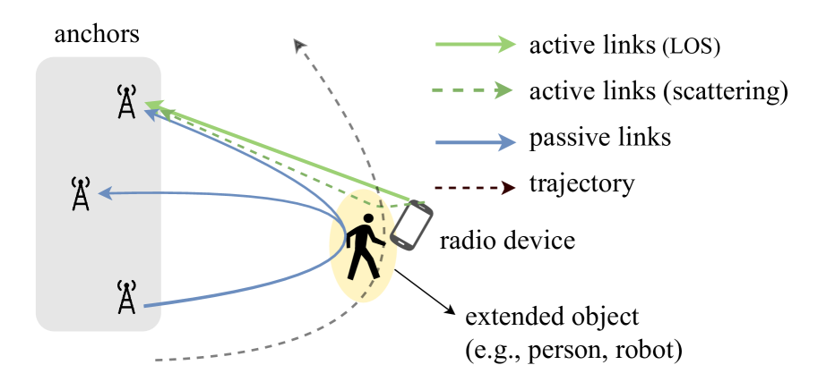
Figure 1: A radio device carried by a person, modeled as an extended object, moves along a trajectory.

This paper presents a radio localization approach for extended object tracking in obstructed line-of-sight (OLOS) scenarios. We propose a Bayesian estimation algorithm which fuses active measurements between a radio device and multiple anchor nodes (fixed radio transceivers with known position) as well as passive measurements in-between anchors reflected off the EO as illustrated in Fig. 1. The algorithm estimates both the radio device’s position and the object’s extent using position-related information from LOS and scattering components. An efficient geometry-based scattering model is proposed to overcome the computational complexity of the ideal scattering model, while still allowing to fuse the scattering information from multiple anchors to jointly estimate the object’s extent. Additionally, an extended object probabilistic data association (EOPDA) algorithm addresses the limitation of the point assumption PDA, improving positioning accuracy.

II Radio Signal Model

At each time step $n$, a radio device at position $\bm{m}_{n}$ transmits a signal, and each anchor $j\hskip-0.85358pt\hskip-0.85358pt\in\hskip-0.85358pt\hskip-0.85358pt\{1,\hskip 0.5pt...\hskip 0.5pt,J\}$ at position $\bm{p}_{\text{a}}^{(j)}=[p_{\text{ax}}^{(j)}\;p_{\text{ay}}^{(j)}]^{\text{T}}$ acts as a receiver, capturing active measurements. Synchronously, pairs of anchors $(j,j^{\prime})$ exchange signals, capturing passive measurements from the EO. The EO, centered at position $\bm{p}_{n}$, is rigidly coupled to the radio device. The gap between the device and the EO’s center is described by the bias $\bm{b}_{n}$. An example is shown in Fig. 2a. We assume scatterers are primarily distributed on the EO’s surface, with the corresponding sector treated as a scattering volume[14]. We denote the scattering volume for active and passive measurements as $\bm{Q}_{\text{A},n}^{(j)}$ and $\bm{Q}_{\text{P},n}^{(j,j^{\prime})}$ for received anchor $j$ at time $n$. Each point-source scatterer is denoted by its position $\bm{q}\in\bm{Q}_{\text{A},n}^{(j)}$ and $\bm{q^{\prime}}\in\bm{Q}_{\text{P},n}^{(j,j^{\prime})}$, respectively[15].

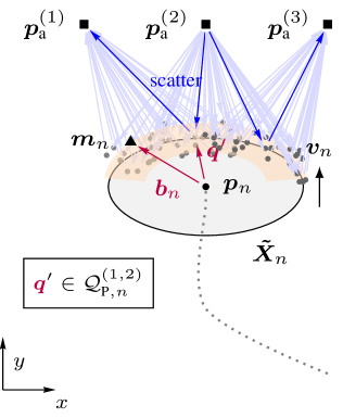
(a)

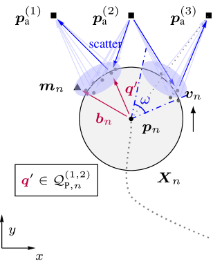
(b)

Figure 2: Scattering models of the extended object for passive measurements. (a) an ideal scattering model where scatterers are distributed within a sector on the EO’s surface, (b) a simplified geometry-based scattering model exploiting the geometric relation of scatterers and the EO.

II-A Active Radio Signal

At each time $n$, a radio signal is transmitted from the radio device and received at anchor $j$. The complex baseband signal from anchor $j$ is modeled as

$$r_{\text{A},n}^{(j)}(t) =\alpha_{n}^{(j)}s(t-\tau_{n}^{(j)})$$

$$\hskip 19.91692pt+\sum_{\bm{q}\in\bm{Q}_{\text{A},n}^{(j)}}\alpha_{\bm{q},n}^{(j)}s(t-\tau_{\bm{q},n}^{(j)})+w_{n}^{(j)}(t)$$ (1)

where $\alpha_{n}^{(j)}$ and $\tau_{n}^{(j)}$ are the complex amplitude and delay of the LOS component from active measurements. The complex amplitude and delay of the scatter component are denoted as $\alpha_{\bm{q},n}^{(j)}$ and $\tau_{\bm{q},n}^{(j)}$ The second term $w_{n}^{(j)}(t)$ accounts for measurement noise modeled as additive white Gaussian noise (AWGN) with double-sided power spectral density $N_{0}/2$.

II-B Passive Radio Signal

At each time step $n$, a radio signal is transmitted from anchor $j^{\prime}$ and received at anchor $j$. The complex baseband signal from anchor $j$ is modeled as

$$r_{\text{P},n}^{(j,j^{\prime})}(t)=\sum_{\bm{q^{\prime}}\in\bm{Q}_{\text{P},n}^{(j,j^{\prime})}}\alpha_{\bm{q^{\prime}},{n}}^{(j,j^{\prime})}s(t-\tau_{\bm{q^{\prime}},{n}}^{(j,j^{\prime})})+w_{n}^{(j,j^{\prime})}(t)$$ (2)

where $\alpha_{\bm{q^{\prime}},{n}}^{(j,j^{\prime})}$ and $\tau_{\bm{q^{\prime}},{n}}^{(j,j^{\prime})}$ are the complex amplitude and delay of the scatter component from $\bm{Q}_{\text{P},n}^{(j,j^{\prime})}$.

II-C Signal Parameter Estimation

Measurements which are extracted using a channel estimation algorithm [4] from active radio signals are called active measurements $\bm{z}_{\text{A},n}$, while measurements which are extracted from passive radio signals are called passive measurements $\bm{z}_{\text{P},n}$. We define the vectors $\bm{z}_{\text{A},n}=[{\bm{z}_{\text{A},n}^{(1)}}^{\text{T}}\cdots{\bm{z}_{\text{A},n}^{(J)}}^{\text{T}}]^{\text{T}}$ and $\bm{z}_{\text{P},n}=[{\bm{z}_{\text{P},n}^{(1,1)}}^{\text{T}}\cdots{\bm{z}_{\text{P},n}^{(J,J)}}^{\text{T}}]^{\text{T}}$ for the measurement vectors per time $n$. Take the passive case for example, we define $\bm{z}^{(j,j^{\prime})}_{\text{P},n}=[\bm{z}^{(j,j^{\prime})}_{\text{P},n,1},\dots\,,\bm{z}^{(j,j^{\prime})}_{\text{P},n,M_{\text{P},n}^{(j,j^{\prime})}}]$ with $M_{\text{P},n}^{(j,j^{\prime})}$ being the number of passive measurements. Each passive measurement $\bm{z}^{(j,j^{\prime})}_{\text{P},n,l}=[z_{\text{P},\text{d},n,l}^{(j,j^{\prime})}~z_{\text{P},\text{u},n,l}^{(j,j^{\prime})}]^{\text{T}}$, $l\in\{1,\,\dots\,M_{\text{P},n}^{(j,j^{\prime})}\}$ contains a distance measurement $z_{\text{P},\text{d},n,l}^{(j,j^{\prime})}\in[0,d_{\text{max}}]$ and a normalized amplitude measurement $z_{\text{P},\text{u},n,l}^{(j,j^{\prime})}\in[\gamma,\infty)$.

III System Model

In this section, we formulate a Bayesian method which fuses multiple object-related measurements from both active and passive measurement data. We jointly estimate the kinematic states as well as the extent states of the EO to address the extended object tracking problem.

At time $n$, the radio device and the extended object are characterized by the kinematic state, bias state and extent state. The kinematic state $\bm{x}_{n}=[\bm{p}_{n}^{\text{T}}\;\bm{v}_{n}^{\text{T}}]^{\text{T}}$ consists of the position of the EO’s center $\bm{p}_{n}=[p_{\text{x}\hskip 0.5ptn}\;p_{\text{y}\hskip 0.5ptn}]^{\text{T}}$ and the velocity $\bm{v}_{n}=[v_{\text{x}\hskip 0.5ptn}\;v_{\text{y}\hskip 0.5ptn}]^{\text{T}}$. The bias describes the offset between the EO center and the radio device, defined as $\bm{b}_{n}=[b_{\rho\hskip 0.5ptn}\;b_{\phi\hskip 0.5ptn}]^{\text{T}}$, where $b_{\rho}$ is the distance between the EO center and the radio device, and $b_{\phi}$ is the orientation relative to the x-axis of the EO coordinate system. A geometry-based scattering model is proposed to approximate the extent of the EO, as illustrated in Fig. 2b. The EO is approximated as a circle, while the scattering volume is modeled as an ellipse, referred to as scattering ellipse. The extent state ${\bm{X}_{n}}=[r_{n}\;w_{n}]^{\text{T}}$, where $r_{n}$ denotes the circle’s radius, and $w_{n}$ represents the semi-minor axis of the scattering ellipses for all anchors. For simplicity, we define the augmented extended object state as $\bm{y}_{n}=[\bm{x}_{n}^{\text{T}}\;\bm{b}_{n}^{\text{T}}\;\bm{X}_{n}^{\text{T}}]^{\text{T}}$. The state estimate of $\bm{y}_{n}$ is obtained by calculating the minimum mean-square error (MMSE) estimator $\hat{\bm{y}}^{\text{MMSE}}_{n}\,\triangleq\int\hskip-0.85358pt\bm{y}_{n}\,f(\bm{y}_{n}|\bm{z}_{\text{A},1:n},\bm{z}_{\text{P},1:n})\,\mathrm{d}\bm{y}_{n}\,$. The estimation process involves marginalizing the joint posterior distribution, as detailed in Sec.III-D.

III-A LOS Measurement Model

The position of the radio device is given as

$$\bm{m}_{n}=\bm{p}_{n}+\begin{bmatrix}b_{\rho\hskip 0.5ptn}\cos(b_{\phi\hskip 0.5ptn})\\ b_{\rho\hskip 0.5ptn}\sin(b_{\phi\hskip 0.5ptn})\end{bmatrix}\,.$$ (3)

The likelihood function (LHF) of an LOS path is given by

$$f_{\text{LOS}}(\bm{z}^{(j)}_{\text{A},n,l}|\bm{x}_{n},\bm{b}_{n})=f_{\text{N}}(z_{\text{A},\text{d},n,l}^{(j)};h_{\text{LOS}}(\bm{m}_{n},\bm{p}_{\text{a}}^{(j)}),\sigma_{\text{d}}^{2}(z_{\text{A},\text{u},n,l}^{(j)}))$$ (4)

where $f_{\text{N}}(x;\mu,\sigma^{2})$ is the Gaussian PDF, with mean $h_{\text{LOS}}(\bm{m}_{n},\bm{p}_{\text{a}}^{(j)})=\|\bm{m}_{n}-\bm{p}_{\text{a}}^{(j)}\|$ being the LOS distance and variance $\sigma_{\text{d}}^{2}(z^{(j)}_{\text{A},\text{u},n,l})$. The variance is determined from the Fisher information given by $\sigma_{\text{d}}^{2}(z^{(j)}_{\text{A},\text{u},n,l})=c^{2}/(8\,\pi^{2}\,\beta_{\text{bw}}^{2}\,(z^{(j)}_{\text{A},\text{u},n,l})^{2})$, where $\beta_{\text{bw}}$ is the root mean squared bandwidth [16, 17], and $(z^{(j)}_{\text{A},\text{u},n,l})^{2}$ corresponds to the SNR.

III-B Scattering Measurement Model

The scattering LHF conditioned on $\bm{x}_{n}$ and $\bm{X}_{n}$ is a convolution of the noise distribution and the scattering distribution [11]. The LHF of an individual scattering measurement is obtained by integrating out the scattering variables. For the passive measurements $\bm{z}^{(j,j^{\prime})}_{\text{P},n,l}$ it is given as

$$\vskip-8.53581ptf_{\text{P}}(\bm{z}^{(j,j^{\prime})}_{\text{P},n,l}|\bm{x}_{n},{\bm{X}}_{n})=\int f(\bm{z}^{(j,j^{\prime})}_{\text{P},n,l}|\bm{x}_{n},\bm{q}^{\prime})f(\bm{q}^{\prime}|\bm{X}_{n})d\bm{q}^{\prime}$$ (5)

The proposed geometry-based scattering model approximates the scattering distribution in (5) as follows. For each received anchor $j$, the center $\bm{\chi}_{n}^{(j)}$ of the scattering ellipse is represented as

$$\bm{\chi}_{n}^{(j)}=\bm{p}_{n}+\begin{bmatrix}r_{n}\cos(\phi_{n}^{(j)})\\ r_{n}\sin(\phi_{n}^{(j)})\end{bmatrix}$$ (6)

where $\phi_{n}^{(j)}$ is the angle between the x-axis of the EO coordinate system and the line from $\bm{p}_{n}$ to $\bm{p}_{\text{a}}^{(j)}$ given as $\phi_{n}^{(j)}=\text{atan2}(\frac{p_{\text{y}\hskip 0.5ptn}-{p}_{\text{a}\hskip 0.5pt\text{y}}^{(j)}}{p_{\text{x}\hskip 0.5ptn}-{p}_{\text{a}\hskip 0.5pt\text{x}}^{(j)}})$. While the unified semi-minor axis $w_{n}$ of all scattering ellipses (contained in $\bm{X}_{n}$) is jointly estimated, the semi-major axis $l_{n}^{(j)}$ is determined by the opening angle $\omega$, symmetric to the line connecting $\bm{p}_{n}$ to $\bm{p}_{\text{a}}^{(j)}$ (see Fig. 2b), capturing scatterers from each anchor $j$. The orientation $\theta_{n}^{(j)}$ of the scattering ellipse follows the circle’s tangent direction. The measurement covariance can be represented as $\bm{R}_{n}^{(j)}=\bm{A}_{n}^{(j)}\bm{E}_{n}^{(j)}{\bm{A}_{n}^{(j)}}^{\text{T}}$, while $\bm{E}_{n}^{(j)}\in\mathbb{R}^{2\times 2}$ is a symmetric, positive semidefinite matrix that describes the 2-D scattering ellipse, and $\bm{A}_{n}^{(j)}$ is the rotation matrix related to $\theta_{n}^{(j)}$. We denote the larger eigenvalue of $\bm{E}_{n}^{(j)}$ as $e_{1}$ and the smaller ones as $e_{2}$. It is assumed that the square root of these eigenvalues is proportional to the volume’s semi-axis [14]. This leads to

$$l_{n}^{(j)}=2\sqrt{e_{1}}~~~\text{and}~~~w_{n}=2\sqrt{e_{2}}$$ (7)

Take the passive case for example, the measurement covariance $\bm{R}_{n}^{(j)}$ is used to decide the covariance matrix of a Gaussian PDF that models the scattering distribution due to the geometric shape as $f(\bm{\zeta}|\bm{R}_{n}^{(j)})\,\triangleq f_{\text{N}}(\bm{\zeta};\bm{0},\bm{R}_{n}^{(j)})$. The LHF of an individual scattering measurement is derived as

$$f_{\text{P(geo)}}(\bm{z}^{(j,j^{\prime})}_{\text{P},n,l}|\bm{x}_{n},\bm{X}_{n})$$

$$=\int f(\bm{z}^{(j,j^{\prime})}_{\text{P},n,l}|\bm{\chi}_{n}^{(j)},\bm{\zeta})f(\bm{\zeta}|\bm{R}_{n}^{(j)})d\bm{\zeta}$$

$$=f_{\text{N}}(z_{\text{P},\text{d},n,l}^{(j,j^{\prime})};{h}_{\text{P}}(\bm{\chi}_{n}^{(j)},\bm{p}_{\text{a}}^{(j^{\prime})},\bm{p}_{\text{a}}^{(j)}),\sigma_{\text{d}}^{2}(z_{\text{P},\text{u},n,l}^{(j,j^{\prime})})+\sigma_{\lambda}^{2})$$ (8)

where ${h}_{\text{P}}(\bm{\chi}_{n}^{(j)},\bm{p}_{\text{a}}^{(j^{\prime})},\bm{p}_{\text{a}}^{(j)})=\|\bm{\chi}_{n}^{(j)}-\bm{p}_{\text{a}}^{(j^{\prime})}\|+\|\bm{\chi}_{n}^{(j)}-\bm{p}_{\text{a}}^{(j)}\|$. The unscented transformation (UT)[19] is applied to transform the propagation uncertainty of the scattering distribution $f(\bm{\zeta}|\bm{R}_{n}^{(j)})$ from position domain to delay domain. The variance $\sigma_{\lambda}^{2}$ represents the dispersion of the sigma points transformed through the nonlinear function $h_{\text{P}}(\cdot)$.

III-C Data Association Uncertainty

For each anchor $j$, the measurements $\bm{z}_{\text{A},n}^{(j)}$ and $\bm{z}_{\text{P},n}^{(j,j^{\prime})}$ are subject to data association uncertainty. Specifically, it is unknown whether a given measurement corresponds to the LOS path, the extended object, or is a result of clutter. To address this uncertainty, the association variables $a_{\text{A},n,l}^{(j)}\in\{0,1\}$ and $a_{\text{P},n,l}^{(j,j^{\prime})}\in\{0,1\}$ are introduced, where a value of $1$ indicates that a measurement is LOS or object-related, while a value of $0$ indicates otherwise. Object-related and clutter measurements follow Poisson distribution with means $\mu_{\text{m}}$ and $\mu_{\text{c}}$. Clutter measurements are independent and uniformly distributed according to $f_{c}(\bm{z}_{\text{A},n,l}^{(j)})$ and $f_{c}(\bm{z}_{\text{P},n,l}^{(j,j^{\prime})})$.

III-D Joint Posterior PDF

It is assumed that the state $\bm{y}_{n}$ evolves over time $n$ as an independent first-order Markov process. Therefore, the joint state transition probability density function (PDF) can be represented as

$$f(\bm{y}_{n}|\bm{y}_{n-1})=f(\bm{x}_{n}|\bm{x}_{n-1})f(\bm{b}_{n}|\bm{b}_{n-1})f(\bm{X}_{n}|\bm{X}_{n-1})$$ (9)

where $f({\bm{x}}_{n}|{\bm{x}}_{n-1})$, $f(\bm{b}_{n}|\bm{b}_{n-1})$ and $f(\bm{X}_{n}|\bm{X}_{n-1})$ are the state transition PDFs of the agent motion, bias and the extent parameters.

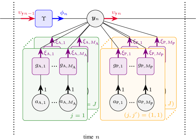
Figure 3: Factor graph representing the factorization of the joint posterior PDF in (10) and the messages according to the SPA. The following short notations are used: $M_{\text{A}}\triangleq M_{\text{A},n}^{(j)}$, $M_{\text{P}}\triangleq M_{\text{P},n}^{(j)}$, $a_{\text{A},l}\triangleq a_{\text{A},n,l}^{(j)}$, $a_{\text{P},l}\triangleq a_{\text{P},n,l}^{(j,j^{\prime})}$, ${g}_{\text{A},l}\triangleq{g}_{\text{A},n,l}^{(j)}$, ${g}_{\text{P},l}\triangleq{g}_{\text{P},n,l}^{(j,j^{\prime})}$, $\xi_{\text{A},l}\triangleq\xi_{\text{A},n,l}^{(j)}$, $\xi_{\text{P},l}\triangleq\xi_{\text{P},n,l}^{(j,j^{\prime})}$.

We assume that the measurements $\bm{z}_{\text{A},n}^{(j)}$ and $\bm{z}_{\text{P},n}^{(j,j^{\prime})}$ are observed and thus fixed. According to the Bayes’s rule and the related independence assumptions, the joint posterior PDF of all estimated states for time $n$ and all $J$ anchors can be derived as

$$f(\bm{y}_{0:n},\bm{a}_{\text{A},{1:n}},\bm{a}_{\text{P},{1:n}}|\bm{z}_{\text{A},{1:n}},\bm{z}_{\text{P},{1:n}})$$

$$\propto f(\bm{y}_{0})\prod_{n^{\prime}=1}^{n}\Upsilon(\bm{y}_{n^{\prime}}|\bm{y}_{n^{\prime}-1})\times\prod_{j=1}^{J}\prod_{l=1}^{M_{\text{A},n^{\prime}}^{(j)}}{g}_{\text{A}}(\bm{z}_{\text{A},n^{\prime},l}^{(j)}|\bm{y}_{n^{\prime}},a_{\text{A},n^{\prime},l}^{(j)})$$

$$\hskip 17.07164pt\times\prod_{j^{\prime}=1}^{J}\prod_{l=1}^{M_{\text{P},n^{\prime}}^{(j,j^{\prime})}}{g}_{\text{P}}(\bm{z}_{\text{P},n^{\prime},l}^{(j,j^{\prime})}|\bm{y}_{n^{\prime}},a_{\text{P},n^{\prime},l}^{(j,j^{\prime})})$$ (10)

where $\Upsilon(\bm{y}_{n}|\bm{y}_{n-1})\,\triangleq f(\bm{y}_{n}|\bm{y}_{n-1})$. Fig. 3 is the factor graph that represents the factorization of (10). The pseudo-likelihood function for the passive case is represented as

$${g}_{\text{P}}(\bm{z}_{\text{P},n,l}^{(j,j^{\prime})}|\bm{y}_{n},a_{\text{P},n,l}^{(j,j^{\prime})})=\begin{cases}\frac{\mu_{m}f_{\text{P}}(\bm{z}_{\text{P},n,l}^{(j,j^{\prime})}|\bm{x}_{n},\bm{X}_{n})}{\mu_{c}f_{c}(\bm{z}_{\text{P},n,l}^{(j,j^{\prime})})},&\text{$a_{\text{P},n,l}^{(j,j^{\prime})}=1$}\\ 1,&\text{$a_{\text{P},n,l}^{(j,j^{\prime})}=0$}\end{cases}$$ (11)

To estimate the states, marginalization of the joint posterior is performed by message passing on the factor graph in Fig. 3 using the sum-product algorithm (SPA)[20] and a particle-based implementation similar to [4].

IV Ideal Scattering Model

For comparison, we also approximate the scattering distribution (5) based on the ideal scattering model in Fig. 2a, where the EO is represented as an ellipse with scatterers distributed within a sector on its surface. The extent state $\bm{\tilde{X}}_{n}=[a_{n}\;b_{n}\;w_{n}]^{\text{T}}$, where $a_{n}$, $b_{n}$ denote the semi-major axis and the semi-minor axis of the EO, respectively, and $w_{n}$ represents the width of the sector. The scattering LHF is approximated by a Monte Carlo technique sampling within the sector to evaluate the integral

$$f_{\text{P(idl)}}(\bm{z}^{(j,j^{\prime})}_{\text{P},n,l}|\bm{x}_{n},{\bm{\tilde{X}}}_{n})$$ (12)

$$\approx\frac{1}{I^{\prime}}\sum_{i=1}^{I^{\prime}}f_{\text{N}}(z_{\text{P},\text{d},n,l}^{(j,j^{\prime})};\bar{h}_{\text{P}}(\bm{x}_{n},\bm{q}^{\prime}_{i},\bm{p}_{\text{a}}^{(j^{\prime})},\bm{p}_{\text{a}}^{(j)}),\sigma_{\text{d}}^{2}(z_{\text{P},\text{u},n,l}^{(j,j^{\prime})}))$$

where $\bar{h}_{\text{P}}(\bm{x}_{n},\bm{q}^{\prime}_{i},\bm{p}_{\text{a}}^{(j^{\prime})},\bm{p}_{\text{a}}^{(j)})=\|(\bm{p}_{n}+\bm{q}^{\prime}_{i})-\bm{p}_{\text{a}}^{(j^{\prime})}\|+\|(\bm{p}_{n}+\bm{q}^{\prime}_{i})-\bm{p}_{\text{a}}^{(j)}\|$, $\bm{q}^{\prime}_{i}$ is the random sample generated in the sector, and $I^{\prime}$ is the number of the samples used per received anchor.

V Results

V-A Simulation Setup

The proposed algorithm is evaluated using synthetic measurements generated according to the scenario presented in Fig. 4 and the radio signal models introduced in Section II. The EO moves along a smooth trajectory featuring two direction changes. A radio device is rigidly coupled to the EO with $b_{\rho}=0.32\,\mathrm{m}$ and $b_{\phi}=-\pi/3$. The generative model follows the ideal scattering model with $\bm{\tilde{X}}$, where $a=0.3\,\mathrm{m}$, $b=0.2\,\mathrm{m}$, and $w=0.1\,\mathrm{m}$. The opening angle is set to $\omega=2\pi/3$. The mean number of scattering measurements and clutter are $\mu_{m}=5$ and $\mu_{c}=5$, respectively. The normalized amplitudes are set to $30$ dB at a $1\,\mathrm{m}$ LOS distance and follow free-space pathloss. The object is observed at $180$ discrete time steps at a constant observation rate of $\Delta T=100\,\mathrm{ms}$. Active measurements are entirely missed for anchors [A1, A2, A3] during time steps $[31,60]$ and $[111,130]$, for [A1, A2] during $[61,80]$, and for [A2] during $[81,110]$, while passive paths from all anchors remain available throughout the trajectory.

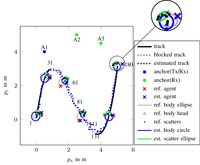
Figure 4: Graphical representation of the synthetic trajectory and one realization of AP-EOPDA(geo) method. The scatters are generated with respect to one received anchor at position $(4,4.5)$ for each time.

The state transition PDF of the kinematic state $f({\bm{x}}_{n}|{\bm{x}}_{n-1})$ is described by a linear, constant velocity and stochastic acceleration model[21, p. 273], given as ${\bm{{x}}}_{n}=\bm{A}\,{\bm{{x}}}_{n\hskip-0.85358pt-\hskip-0.85358pt1}+\bm{B}\,\bm{{w}}_{n}$. The acceleration process $\bm{{w}}_{n}$ is i.i.d. across $n$, zero mean, and Gaussian with covariance matrix ${\sigma_{\text{a}}^{2}}\,\bm{I}_{2}$, with ${\sigma_{\text{a}}}$ being the acceleration standard deviation, and $\bm{A}\in\mathbb{R}^{\text{4x4}}$ and $\bm{B}\in\mathbb{R}^{\text{4x2}}$ are defined according to [21, p. 273]. Furthermore, the state transition PDF of the bias state is factorized as $f(\bm{b}_{n}|\bm{b}_{n-1})=f({b}_{\rho\hskip 0.5ptn}|{{b}}_{\rho\hskip 0.5pt{n-1}})f({b}_{\phi\hskip 0.5ptn}|{b}_{\phi\hskip 0.5pt{n-1}})$. The PDFs of ${b}_{\rho\hskip 0.5ptn}$ and ${b}_{\phi\hskip 0.5ptn}$ are ${b}_{\rho\hskip 0.5ptn}={b}_{\rho\hskip 0.5ptn-1}+{\varepsilon}_{\rho\hskip 0.5ptn}$ and ${b}_{\phi\hskip 0.5ptn}={b}_{\phi\hskip 0.5ptn-1}+{\varepsilon}_{\phi\hskip 0.5ptn}$, respectively. For the geometry-based scattering model, the state transition PDF of the extent state is factorized as $f(\bm{X}_{n}|\bm{X}_{n-1})=f({r}_{n}|{{r}}_{{n-1}})f({w}_{n}|{w}_{{n-1}})$. The PDFs of ${r}_{n}$ and ${w}_{n}$ are ${r}_{n}={r}_{n-1}+{\varepsilon}_{r\hskip 0.5ptn}$ and ${w}_{n}={w}_{n-1}+{\varepsilon}_{w\hskip 0.5ptn}$, respectively. While the noise ${\varepsilon}_{\rho\hskip 0.5ptn}$, ${\varepsilon}_{\phi\hskip 0.5ptn}$, ${\varepsilon}_{r\hskip 0.5ptn}$ and ${\varepsilon}_{w\hskip 0.5ptn}$ are i.i.d. across $n$, zeros mean, Gaussian, with variances ${\sigma_{{\varepsilon}_{\rho}}^{2}}$, ${\sigma_{{\varepsilon}_{\phi}}^{2}}$, ${\sigma_{{\varepsilon}_{r}}^{2}}$ and ${\sigma_{{\varepsilon}_{w}}^{2}}$, respectively. The number of particles is set to $I=5000$ for inference during the track, and the particles consist of all considered random variables. The state-transition variances are set as ${\sigma_{\text{a}}}=2\,\mathrm{m/s^{2}}$, ${\sigma_{\bm{\varepsilon}_{\rho}}}=0.1\,\mathrm{m}$, ${\sigma_{\bm{\varepsilon}_{\phi}}}=0.5\,\mathrm{rad}$, ${\sigma_{\bm{\varepsilon}_{r}}}=0.05\,\mathrm{m}$, and ${\sigma_{\bm{\varepsilon}_{w}}}=0.05\,\mathrm{m}$.

V-B Performance Evaluation

To evaluate the proposed algorithm, we compare the PDA method under the point assumption, denoted as AP-PDA, with the PDA designed for the extended object, denoted as AP-EOPDA, and a method excluding passive measurements, denoted as A-EOPDA. Additionally, we contrast the proposed geometry-based scattering model with the ideal scattering model, as mentioned in Sec. IV, under the AP-EOPDA method, denoted as AP-EOPDA(geo) and AP-EOPDA(idl) with $I^{\prime}=50$. The posterior Cramér-Rao lower bound (P-CRLB) is provided as a performance baseline considering the dynamic model of the EO state [22]. The P-CRLB* assumes continuous LOS availability to all anchors throughout the trajectory, while the P-CRLB varies based on LOS blockages along the trajectory.

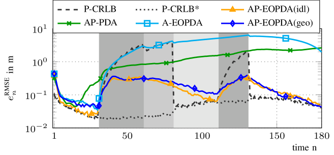
(a)

(b)

Figure 5: Performance of different methods in synthetic measurements described in Fig. 4, (a) is the RMSE of the estimated agent position, and (b) is the cumulative distribution of the RMSE based on numerical simulations. Different shades of grey represent different numbers of blocked anchors described in Sec. V-A.

Fig. 5 provides the results of a numerical simulation with $100$ runs. The root mean squared error (RMSE) of the estimated device’s position is given by Fig. 5a and calculated by $e_{n}^{\text{RMSE}}~=~\sqrt{\mathbb{E}\hskip-1.07639pt\left\{\lVert\hat{\bm{m}}^{\text{MMSE}}_{n}-\bm{m}_{n}\rVert^{2}\right\}}$. Fig. 5b provides the cumulative probability of the position errors ${\|{\hat{\bm{m}}^{\text{MMSE}}_{n}-\bm{m}_{n}}\|}$ evaluated over the whole track. Comparing A-EOPDA with AP-EOPDA, we find that the RMSE of the joint estimation (active & passive) significantly outperforms that of the active-only estimation, particularly during and after the OLOS time steps. AP-EOPDA(idl) precisely attains the P-CRLB before the OLOS situation and converges back to the P-CRLB afterward. In comparison, AP-EOPDA(geo) achieves a similar performance while requiring only half the execution time of the AP-EOPDA(idl) method, as shown in Table I. In contrast, AP-PDA diverges significantly to an incorrect position due to the inadequacy of the single-point assumption for extended object tracking.

TABLE I: Comparison of running time and averaged rmse values of different methods in investigated scenarios.

Models	avg. RMSE (m)	running time per step (s)
AP-EOPDA(geo)	0.18	0.33
AP-EOPDA(idl)	0.16	0.67

VI Conclusion and Future Work

This paper addresses the challenge of achieving robust positioning of a radio device attached with an EO when the LOS between the device and anchors is obstructed by the EO. We propose a joint estimation method that fuses both active and passive measurements from multiple anchors, introducing the probabilistic data association for extended object tracking. Results show that our proposed method significantly reduces the RMSE during and after the obstructed LOS, compared to methods using only active measurements or the point-assumption PDA. The passive measurements provide useful information for estimation, improving positioning accuracy during the full LOS blockage and minimizing outliers after the obstruction. Additionally, the geometry-based extended object model offers substantial computational efficiency, reducing the processing time by $50\,\%$ compared to the ideal scattering model, which is advantageous with an increasing anchor number. Future research will focus on validating the algorithm with real measurement data.

References

- [1] K. Witrisal, P. Meissner, E. Leitinger, Y. Shen, C. Gustafson, F. Tufvesson, K. Haneda, D. Dardari, A. F. Molisch, A. Conti, and M. Z. Win, “High-accuracy localization for assisted living: 5G systems will turn multipath channels from foe to friend,” IEEE Signal Process. Mag., vol. 33, no. 2, pp. 59–70, Mar. 2016.
- [2] E. Leitinger, F. Meyer, F. Hlawatsch, K. Witrisal, F. Tufvesson, and M. Z. Win, “A belief propagation algorithm for multipath-based SLAM,” IEEE Trans. Wireless Commun., vol. 18, no. 12, pp. 5613–5629, Dec. 2019.
- [3] E. Leitinger, A. Venus, B. Teague, and F. Meyer, “Data fusion for multipath-based SLAM: Combining information from multiple propagation paths,” IEEE Transactions on Signal Processing, vol. 71, pp. 4011–4028, 2023.
- [4] A. Venus, E. Leitinger, S. Tertinek, and K. Witrisal, “A graph-based algorithm for robust sequential localization exploiting multipath for obstructed-LOS-bias mitigation,” IEEE Transactions on Wireless Communications, vol. 23, no. 2, pp. 1068–1084, 2024.
- [5] ——, “A message passing based adaptive PDA algorithm for robust radio-based localization and tracking,” in 2021 Proc. IEEE RadarConf-21, 2021, pp. 1–6.
- [6] A. Venus, E. Leitinger, S. Tertinek, F. Meyer, and K. Witrisal, “Graph-based simultaneous localization and bias tracking,” IEEE Trans. Wireless Commun., vol. 23, no. 10, pp. 13 141–13 158, May 2024.
- [7] J. W. Koch, “Bayesian approach to extended object and cluster tracking using random matrices,” IEEE Transactions on Aerospace and Electronic Systems, vol. 44, no. 3, pp. 1042–1059, 2008.
- [8] K. Granström, S. Reuter, D. Meissner, and A. Scheel, “A multiple model PHD approach to tracking of cars under an assumed rectangular shape,” in 17th International Conference on Information Fusion (FUSION), 2014, pp. 1–8.
- [9] M. Baum and U. D. Hanebeck, “Extended object tracking with random hypersurface models,” IEEE Transactions on Aerospace and Electronic Systems, vol. 50, no. 1, pp. 149–159, 2014.
- [10] Y. Bar-Shalom, F. Daum, and J. Huang, “The probabilistic data association filter,” IEEE Control Syst. Mag., vol. 29, no. 6, pp. 82–100, Dec 2009.
- [11] F. Meyer and J. L. Williams, “Scalable detection and tracking of geometric extended objects,” IEEE Trans. Signal Process., vol. 69, pp. 6283–6298, Oct. 2021.
- [12] L. Wielandner, A. Venus, T. Wilding, and E. Leitinger, “Multipath-based SLAM for non-ideal reflective surfaces exploiting multiple-measurement data association,” J. Adv. Inf. Fusion, vol. 18, pp. 59–77, Dec. 2023.
- [13] L. Wielandner, A. Venus, T. Wilding, K. Witrisal, and E. Leitinger, “MIMO multipath-based SLAM for non-ideal reflective surfaces,” in Proc. Fusion-2024, Venice, Italy, Jul. 2024.
- [14] P. Hoher, S. Wirtensohn, T. Baur, J. Reuter, F. Govaers, and W. Koch, “Extended target tracking with a lidar sensor using random matrices and a virtual measurement model,” IEEE Trans. Signal Process., vol. 70, pp. 228–239, Dec. 2022.
- [15] T. Wilding, E. Leitinger, and K. Witrisal, “Multipath-based localization and tracking considering off-body channel effects,” in 2022 16th European Conference on Antennas and Propagation (EuCAP), 2022, pp. 1–5.
- [16] K. Witrisal, E. Leitinger, S. Hinteregger, and P. Meissner, “Bandwidth scaling and diversity gain for ranging and positioning in dense multipath channels,” IEEE Wireless Commun. Lett., vol. 5, no. 4, pp. 396–399, Aug. 2016.
- [17] E. Leitinger, P. Meissner, C. Ruedisser, G. Dumphart, and K. Witrisal, “Evaluation of position-related information in multipath components for indoor positioning,” IEEE J. Sel. Areas Commun., vol. 33, no. 11, pp. 2313–2328, Nov. 2015.
- [18] M. Feldmann, D. Fränken, and W. Koch, “Tracking of extended objects and group targets using random matrices,” IEEE Trans. Signal Process., vol. 59, no. 4, pp. 1409–1420, Sep. 2011.
- [19] E. Wan and R. Van Der Merwe, “The unscented Kalman filter for nonlinear estimation,” in Proc. IEEE ASSPCC 2000, Aug. 2000, pp. 153–158.
- [20] F. Kschischang, B. Frey, and H.-A. Loeliger, “Factor graphs and the sum-product algorithm,” IEEE Trans. Inf. Theory, vol. 47, no. 2, pp. 498–519, Feb. 2001.
- [21] Y. Bar-Shalom, T. Kirubarajan, and X.-R. Li, Estimation with Applications to Tracking and Navigation. New York, NY, USA: John Wiley & Sons, Inc., 2002.
- [22] P. Tichavsky, C. Muravchik, and A. Nehorai, “Posterior Cramer-Rao bounds for discrete-time nonlinear filtering,” IEEE Trans. Signal Process., vol. 46, no. 5, pp. 1386–1396, May 1998.