Finite time blowup for Keller-Segel equation with logistic damping in three dimensions

Abstract.

The Keller-Segel equation, a classical chemotaxis model, and many of its variants have been extensively studied for decades. In this work, we focus on $3$D Keller-Segel equation with a quadratic logistic damping term $-\mu\rho^{2}$ (modeling density-dependent mortality rate) and show the existence of finite-time blowup solutions with nonnegative density and finite mass for any $\mu\in\big{[}0,\frac{1}{3}\big{)}$. This range of $\mu$ is sharp; for $\mu\geq\frac{1}{3}$, the logistic damping effect suppresses the blowup as shown in [40, 60]. A key ingredient is to construct a self-similar blowup solution to a related aggregation equation as an approximate solution, with subcritical scaling relative to the original model. Based on this construction, we employ a robust weighted $L^{2}$ method to prove the stability of this approximate solution, where modulation ODEs are introduced to enforce local vanishing conditions for the perturbation lying in a singular-weighted $L^{2}$ space. As a byproduct, we exhibit a new family of type I blowup mechanisms for the classical $3$D Keller-Segel equation.

1. Introduction

Chemotaxis is a widespread natural phenomenon and it occurs when organisms, such as body cells or bacteria, detect and move toward chemical signals in their surroundings. A principal mathematical description of chemotaxis is provided by the Keller-Segel system:

$$\begin{cases}\partial_{t}\rho=\Delta\rho-\nabla\cdot(\rho\nabla c),\\ \Delta c+\rho=0,\end{cases}$$ (KS)

where $\rho$ represents the density of the bacteria and $c$ denotes the concentration of the self-emitted chemical substance. The model captures two key processes: the diffusive effect of random bacterial motion and the directed movement of bacteria toward the highest concentration of the chemical. For a broader introduction to chemotaxis, see [10, 32, 33].

Biologically, beyond the competition between diffusion and bacterial aggregation, the limitation of resources and overcrowding necessitate introducing the bacterial mortality rate that further suppresses the aggregation process. In particular, we consider the following $3$D coupled parabolic-elliptic Keller-Segel system with logistic damping

$$\begin{cases}\partial_{t}\rho=\Delta\rho-\nabla\cdot(\rho\nabla c)-\mu\rho^{2},\\ \Delta c+\rho=0,\end{cases}$$ (KS-D)

where $-\mu\rho^{2}$ ($\mu\geq 0$) represents the logistic damping rate. For additional background on (KS-D) and related models, we refer the interested readers to [27, 31, 56, 58, 60].

1.1. Background

1.1.1. Classical Keller-Segel equation: global existence v.s. finite-time blowup

For classical Keller-Segel equation (KS), the total mass $M(t)=\int\rho(t,x)dx$ is conserved for all time. Additionally, the system (KS) admits a one-parameter family of scaling invariance:

$$\rho(t,x)\to\frac{1}{\lambda^{2}}\rho\left(\frac{t}{\lambda^{2}},\frac{x}{\lambda}\right),\ c(t,x)\to c\left(\frac{t}{\lambda^{2}},\frac{x}{\lambda}\right),\quad\forall\;\lambda>0.$$ (1.1)

We remark that this scaling invariance also holds for (KS-D).

In two dimensions, the total mass $M=8\pi$ serves as a crucial quantity determining the global existence and finite-time blowup of the system (KS). Specifically, it has been shown that finite-time blowup occurs whenever $M>8\pi$ with initial data $\rho_{0}\in L_{+}^{1}((1+|x|^{2}),dx)$, while global-in-time existence with a uniform $L^{\infty}$ bound holds when $M<8\pi$, see [3, 22].

Nevertheless, the critical mass threshold does not exist for the three-dimensional model (KS). In fact, even with a tiny total mass, there is a radial solution that develops finite-time singularity found by Nagai [50]. Beyond the radial case, Corrias, Perthame, and Zaag [21] demonstrated that blowup occurs whenever the second moment of the initial density is sufficiently small in comparison to the total mass, while weak solutions exist globally if the initial density has a suitably small $L^{\frac{3}{2}}$ norm. Interested readers can refer to [1, 2, 55, 59] for more results.

1.1.2. Classical Keller-Segel equation: singularity formation

Over the last several decades, the singularity formation for the classical Keller-Segel equation (KS) has been well studied. For the $2$D case, since the model is in the $L^{1}$ critical sense, Naito and Suzuki [52] verified that any finite-time blowup solution to (KS) is of type II. In particular, Raphaël and Schweyer [57] provided a precise construction of a radially stable finite-time blowup solution of the form

$$\rho(t,x)\approx\frac{1}{\lambda^{2}(t)}U\left(\frac{x}{\lambda(t)}\right),\quad U(x)=\frac{8}{(1+|x|^{2})^{2}},$$ (1.2)

where the blowup rate

$$\lambda(t)=\sqrt{T-t}e^{-\sqrt{\frac{|\ln(T-t)|}{2}}+O(1)},\quad t\to T.$$

Subsequently, this result has been extended to several refined scenarios, including nonradial blowup, multi-bubble blowup without collision, and the simultaneous collision of two collapsing bubbles. For further details, we refer the interested reader to [7, 17, 19].

Unlike the $2$D case, the $3$D Keller-Segel system exhibits a large variety of blowup mechanisms. Notably, there is a countable family of radial self-similar blowup solutions of the form

$$\rho_{s}(t,x)=\frac{1}{T-t}Q_{s}\left(\frac{x}{\sqrt{T-t}}\right),\;$$ (1.3)

which have been identified in [4, 30, 54]. In particular, there is an explicit self-similar solution given by

$$\rho_{s*}(t,x)=\frac{1}{T-t}Q_{s*}\left(\frac{x}{\sqrt{T-t}}\right),\quad\text{ with }\quad Q_{s*}(x)=\frac{4(6+|x|^{2})}{(2+|x|^{2})^{2}},$$ (1.4)

whose radial stability has been verified by Glogić and Schörkhuber [28]. Recently, Li and the third author [43, 44] extended this stability theory to the nonradial setting. Beyond self-similar blowup solutions, other non-self-similar formations have also been identified. For example, Collot, Ghoul, Masmoudi, and Nguyen [18] discovered a collapsing-ring blowup solution, and Nguyen, Nouaili, and Zaag [53] found a type I blowup solution with a log correction on the shrinking rate. Additionally, Hou, Nguyen and Song [34] recently found a type II blowup solution under axisymmetry, whose local leading-order profile coincides with the rescaled stationary solution of the two-dimensional Keller-Segel equation as given in (1.2).

1.1.3. Blowup or no blowup with logistic damping

To detect the core mechanism behind the bacterial aggregation, we can rewrite the aggregation term in (KS) or (KS-D) as

$$\nabla\cdot(\rho\nabla\Delta^{-1}\rho)=\nabla\Delta^{-1}\rho\cdot\nabla\rho+\rho^{2}.$$

In this expression, $\nabla\Delta^{-1}\rho\cdot\nabla\rho$ is the advection term, which, along with the effect of the diffusion term, cannot lead to the finite-time blowup. Consequently, the main factor causing blowup is $\rho^{2}$.

If the logistic damping term $-\mu\rho^{2}$ in (KS-D) is replaced by a stronger term of the form $-\mu\rho^{p}$ with $\mu>0$ and $p>2$, then the aggregation effect is always suppressed. Thus, the solution always exists globally in time regardless of how concentrated the initial density is, see [60].

In the scenario of quadratic damping $-\mu\rho^{2}$ (corresponding to (KS-D)), Tello and Winkler [60] proved that the global existence is guaranteed for any $\mu>0$ in two dimensions. For higher dimension $d\geq 3$, they further demonstrated that global existence holds provided $\mu>\frac{d-2}{d}$. Subsequently, Kang and Stevens [40] verified the global existence in the critical case $\mu=\frac{d-2}{d}$ with $d\geq 3$. In the subcritical regime with $\mu\in\left(0,\frac{d-2}{d}\right)$, Fuest [27] partially bridged the gap by proving that finite-time blowup occurs in a bounded domain for $\mu\in\left(0,\frac{d-4}{d}\right)$ in higher dimensions $d\geq 5$. However, to the best of the authors’ knowledge, prior to the present work, it remained an open problem whether blowup occurs for $\mu\in(0,\frac{d-4}{d})$ with $d\geq 5$ and $\mu\in(0,\frac{d-2}{d})$ with $3\leq d\leq 4$.

Regarding the weaker damping term $-\mu\rho^{p}$ with $1<p<2$, for higher dimensions $d\geq 5$, Winkler [61] verified the existence of finite-time blowup solution when $1<p<\frac{3}{2}+\frac{1}{2d-2}$. Subsequently, for dimensions $d\in\{3,4\}$, Winkler [62] demonstrated finite-time blowup for $1<p<\frac{7}{6}$. This range was later significantly extended by Fuest [27], where the author established the finite-time blowup for $1<p<\frac{3}{2}$ in dimensions $d=3$ and for $1<p<2$ in dimensions $d\geq 4$, thereby completing the finite-time blowup theory in the high-dimensional regime $d\geq 4$.

1.2. Main result

The principal objective of this work is to establish the optimal blowup result to (KS-D) in three dimensions. Specifically, we establish the existence of a smooth finite-time blowup solution to (KS-D) with nonnegative density and finite mass for any $0\leq\mu<\frac{1}{3}$ in three dimensions.

In the literature, most blowup results for chemotaxis equations are obtained either by tracking the evolution of some appropriate functional (such as the second moment) to obtain a contradiction [3, 21, 22], or by working in the radial setting where the mass accumulation function satisfies an ODE [27]. However, the damping term $-\mu\rho^{2}$ in (KS-D) destroys the structures that these proofs rely on. In particular, it leads to a time-decreasing mass and breaks the divergence form structure that the classical Keller-Segel equation (KS) enjoys, thereby making these classical methods too limited to obtain the sharp blowup result for (KS-D).

Motivated by the various singularity formation results, ranging from the nonlinear heat equation [5, 20, 35, 49], nonlinear wave equation [23, 41], nonliear Schrödinger equation [45, 48], incompressible fluids [13, 14, 15, 36, 24, 25], compressible fluids [6, 12, 47], we adopt a strategy based on the direct construction of finite-time blowup solutions via the stability analysis of an approximate blowup solution. And the precise statement of the main theorem is as follows:

Theorem 1.1 (Existence of finite-time blowup to (KS-D) with finite mass).

For any fixed $0\leq\mu<\frac{1}{3}$, let $j_{0}$ be an integer such that

$$j_{0}\geq J:=\frac{3(1-\mu)}{1-3\mu}+1>1,$$ (1.5)

it then follows that

$$\beta=\beta(j_{0},\mu):=\frac{1}{3(1-\mu)}+\frac{1}{2j_{0}}<\frac{1}{2}.$$ (1.6)

In addition, under these choices, there exists a radially nonnegative $\rho_{0}\in C_{0}^{\infty}(\mathbb{R}^{3})$ such that the related smooth solution to (KS-D) exhibits finite-time blowup at $t=T<\infty$. Moreover, the solution satisfies

$$\rho(t,x)=\frac{1}{T-t}\left[Q\left(\frac{x}{(T-t)^{\beta}}\right)+\varepsilon\left(t,\frac{x}{(T-t)^{\beta}}\right)\right],\quad x\in\mathbb{R}^{3},\;t\in[0,T),$$ (1.7)

where

$\bullet$ (Existence of profile). $Q$ is a unique smooth radial decreasing solution to the equation:

$$Q+\beta y\cdot\nabla_{y}Q=\nabla_{y}Q\cdot\nabla_{y}\Delta^{-1}_{y}Q+(1-\mu)Q^{2},$$ (1.8)

with the initial data

$$Q(0)=\frac{1}{1-\mu}\quad\text{ and }\quad\partial_{r}^{(2j_{0})}Q(0)=-(2j_{0})!<0.$$ (1.9)

$\bullet$ (Smallness of error term). There exists $s=s(\mu)\in\mathbb{Z}_{\geq 1}$ sufficiently large and constants $C>0$ and $\bar{\epsilon}>0$ such that the error term $\varepsilon$ satisfies

$$\|\varepsilon(t)\|_{H^{s}(\mathbb{R}^{3})}\leq C\left(T-t\right)^{\bar{\epsilon}},\quad\forall\;0\leq t<T.$$

Comments on Theorem 1.1.

$1.$ Optimality in blowup results for Keller-Segel equation with logistic damping.

Theorem 1.1 shows the existence of finite-time blowup solution to $3$D Keller-Segel equation with logistic damping (KS-D) for any fixed $0\leq\mu<\frac{1}{3}$. This result provides the optimal blowup threshold for (KS-D) and completes the long-standing conjecture proposed in [27, 60] as mentioned in Subsection 1.1.3.

Moreover, our method is robust enough to extend naturally to higher dimensions $d\geq 3$, resulting in an analogous sharp blowup regime. Specifically, for $\mu\in\Big{[}0,\frac{d-2}{d}\Big{)}$ with $d\geq 3$, there always exists a finite-time blowup solution to (KS-D).

When the damping term is weakened to $-\mu\rho^{p}$ with $\mu>0$ and $1\leq p<2$, the problem becomes simpler, as this term can be viewed primarily as a perturbation of the dominant aggregation effect as well. Concretely, one could use $\frac{1}{T-t}Q\big{(}\frac{x}{(T-t)^{\beta}}\big{)}$ with $Q$ constructed in Theorem 1.1 with $\mu=0$ as an approximate solution. Alternatively, one may use the self-similar solution (1.4) of the classical Keller-Segel equation (KS) as an approximate solution. Then, we could apply the stability theory developed in this work or [28, 44] to establish the existence of finite-time blowup for any $\mu>0$ and $p\in[1,2)$ in three dimensions.

$2.$ New blowup mechanism for classical Keller-Segel equation in $3$D.

For $3$D classical Keller-Segel equation (KS), by applying Theorem 1.1 with $\mu=0$, we have constructed a countably infinite family of blowup solutions, whose asymptotic behavior is given by

$$\rho(t,x)\approx\frac{1}{T-t}Q_{\beta_{j}}\left(\frac{x}{(T-t)^{\beta_{j}}}\right),\qquad\forall\;t\in(0,T),$$

where $\beta_{j}=\frac{1}{3}+\frac{1}{2j}<\frac{1}{2}$ for all $j\geq 4$ and each $Q_{\beta_{j}}$ solves (1.8) with $\beta=\beta_{j}$. This blowup is an "abnormal" Type I blowup, in the sense that it does not match natural scaling (1.1) . Consequently, as a by-product of Theorem 1.1, we establish a family of new blowup mechanisms for $3$D classical Keller-Segel equation (KS).

$3.$ Extension of Theorem 1.1.

Theorem 1.1 establishes the precise blowup mechanism for the density but does not address its stability. Nevertheless, by following the standard approach outlined in [20, 44], one can construct a finite-codimensional Lipschitz stable manifold of radial initial data such that the corresponding solutions to (KS-D) exhibit blowup dynamics similar to in (1.7).

Besides, a natural extension to the nonradial blowup can be expected by using the spectral method from [8, 9, 11, 12]. Alternatively, following the argument in [16], one might introduce a matrix system of modulation ODEs to realize it. Furthermore, noting that the blowup solution constructed in Theorem 1.1 is highly localized, one can expect a finite-time blowup solution in a bounded domain by adapting the cut-off technique from [8, 9]. However, as the main focus of this work is on the existence of finite-time blowup solutions to (KS-D), we do not pursue these generalizations in detail here.

In addition, our method is expected to be sufficiently robust to potentially shed light on other models, such as the nonlinear heat equations. As a further motivation for the linear and nonlinear analysis for the Keller-Segel equation (KS-D) in Section 4 and Section 5, we briefly outline this in Section 2 for $1$D semilinear heat equation.

1.3. Proof strategy and related key highlights.

1.3.1. Key idea of the construction: diffusion term as perturbation.

Motivated by the well-known explicit self-similar blowup solution (1.4) to the classical Keller-Segel equation (KS), a direct idea is to seek an analogous self-similar solution matching the natural scaling for the damped system (KS-D). Specifically, since (KS-D) satisfies the scaling invariance (1.1) as well, one is led to consider special solutions of the form

$$\rho_{\mu}(t,x)=\frac{1}{T-t}Q_{\mu}\left(\frac{x}{\sqrt{T-t}}\right),$$

where $Q_{\mu}$ solves

$$Q_{\mu}+\frac{1}{2}y\cdot\nabla Q_{\mu}=\Delta Q_{\mu}+\nabla\cdot(Q_{\mu}\nabla\Delta^{-1}Q_{\mu})-\mu Q_{\mu}^{2}.$$ (1.10)

However, the damping term $-\mu\rho^{2}$ significantly complicates the problem by breaking the divergence structure of (KS). In particular, the partial mass

$$m_{\rho}(r):=\int_{B(0,r)}\rho(x)dx,$$ (1.11)

is invalid to simplify the equation (1.10) into a second order local differential equation, resulting (1.10) essentially a third-order differential equation for general $\mu\in\left(0,\frac{1}{3}\right)$, which, to the best of authors’ knowledge, is quite difficult to analyze and is still open.

Instead, we adopt an alternative approach inspired by [16, 35, 46, 47, 53], where the first step is to neglect the diffusion term and construct a self-similar blowup solution for the following $3$D aggregation equation

$$\partial_{t}\rho=\nabla\rho\cdot\nabla\Delta^{-1}\rho+(1-\mu)\rho^{2},$$ (1.12)

in the form

$$\rho(t,x)=\frac{1}{T-t}Q\left(\frac{x}{(T-t)^{\beta}}\right),\;\text{ with }\beta<\frac{1}{2},$$ (1.13)

where the profile $Q$ satisfies (1.8). We then choose (1.13) as an approximate solution to the original system (KS-D), which breaks the natural scaling of (KS-D), thus making the diffusion term $\Delta\rho$ subcritical and allowing it to be treated as a perturbation relative to the dominant aggregation term.

Compared to (1.10), the equation (1.8) is effectively second-order and much more tractable. By restricting onto radial solutions and introducing the averaged mass of $Q$ in the ball $B(0,r)$

$$f_{Q}(r):=\frac{1}{r^{3}}\int_{0}^{r}Q(s)s^{2}ds,$$ (1.14)

(1.8) can be reformulated as an ODE system in terms of $(Q,f_{Q})$ (see (3.3)). The existence of solutions to (1.8) follows directly from a standard phase portrait analysis (See Figure 3 and Lemma 3.2). This method has been instrumental in recent developments concerning the construction of smooth profiles for implosion, gravitational collapse, and collapsing-expanding shocks [6, 29, 37, 38, 47]. The regularity of self-similar solutions serves as a fundamental criterion for solution admissibility and plays a crucial role in ensuring the existence of a nontrivial solution in the context of the present problem.

1.3.2. Compatibility of $\mu<\frac{1}{3}$: insights from the phase portrait analysis.

One of the main goals of our paper is to figure out the existence of the smooth nontrivial radial solution to (1.8) for some $\beta<\frac{1}{2}$, which can be further simplified into finding a smooth curve connecting

$$P_{0}:=\left(\frac{1}{1-\mu},\frac{1}{3(1-\mu)}\right),$$ (1.15)

and the origin $O$ under the ODE system for $(Q,f_{Q})$ given by (3.3). We classify the problem into three cases based on the relative position of $f_{Q}=\beta$ and $P_{0}$, and analyze the corresponding phase portraits:

Case I. $P_{0}$ lies strictly above the line $\{f_{Q}=\beta\}$: $\beta<\frac{1}{3(1-\mu)}$ (See Figure 1).

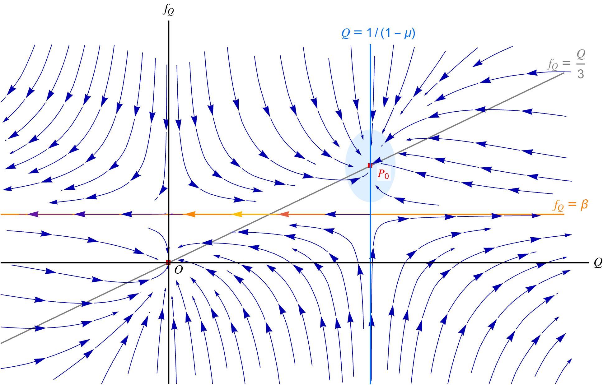
Figure 1. $Qf_{Q}$-plane with $P_{0}$ above the line $f_{Q}=\beta$. In this case, there is only a trivial solution solving (3.3) with $(Q(0),f_{Q}(0))=P_{0}$.

We remark here that in Case I $\big{(}\beta<\frac{1}{3(1-\mu)}\big{)}$, motivated by the related phase portrait (see Figure 1), the flow field around $P_{0}$ is directed toward $P_{0}$. Consequently, $P_{0}$ is a stagnant point in this case and $Q(r)\equiv\frac{1}{1-\mu}$ is the only smooth solution to (3.3) with $(Q(0),f_{Q}(0))=P_{0}$ that can be obtained. Therefore, to obtain a nontrivial solution to (3.3) with $(Q(0),f_{Q}(0))=P_{0}$, it is necessary for $\beta$ to satisfy

$$\frac{1}{3(1-\mu)}\leq\beta<\frac{1}{2}.$$ (1.16)

This requires that $\mu<\frac{1}{3}$, which aligns exactly with the optimal range of $\mu$ provided in Subsection 1.1.3 and Theorem 1.1.

Case II. $P_{0}$ lies on the line $\{f_{Q}=\beta\}$: $\beta=\frac{1}{3(1-\mu)}$ (See Figure 2).

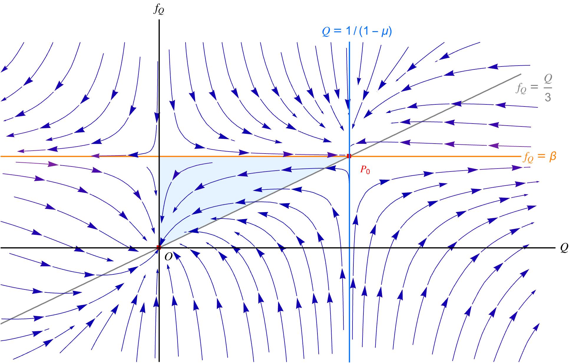
Figure 2. $Qf_{Q}$-plane with $P_{0}$ on the line $f_{Q}=\beta$. In this case, though it seems possible to have a solution curve connecting between $P_{0}$ and the origin $O$ from the phase portrait, with the overwhelming singularity on the right-hand side of (3.3), after some careful analysis, the only possible smooth solution starting from $P_{0}$ to should be the trivial one: $(Q(r),f_{Q}(r))\equiv P_{0}$.

Case III. $P_{0}$ lies strictly below the line $\{f_{Q}=\beta\}$: $\beta>\frac{1}{3(1-\mu)}$ (See Figure 3).

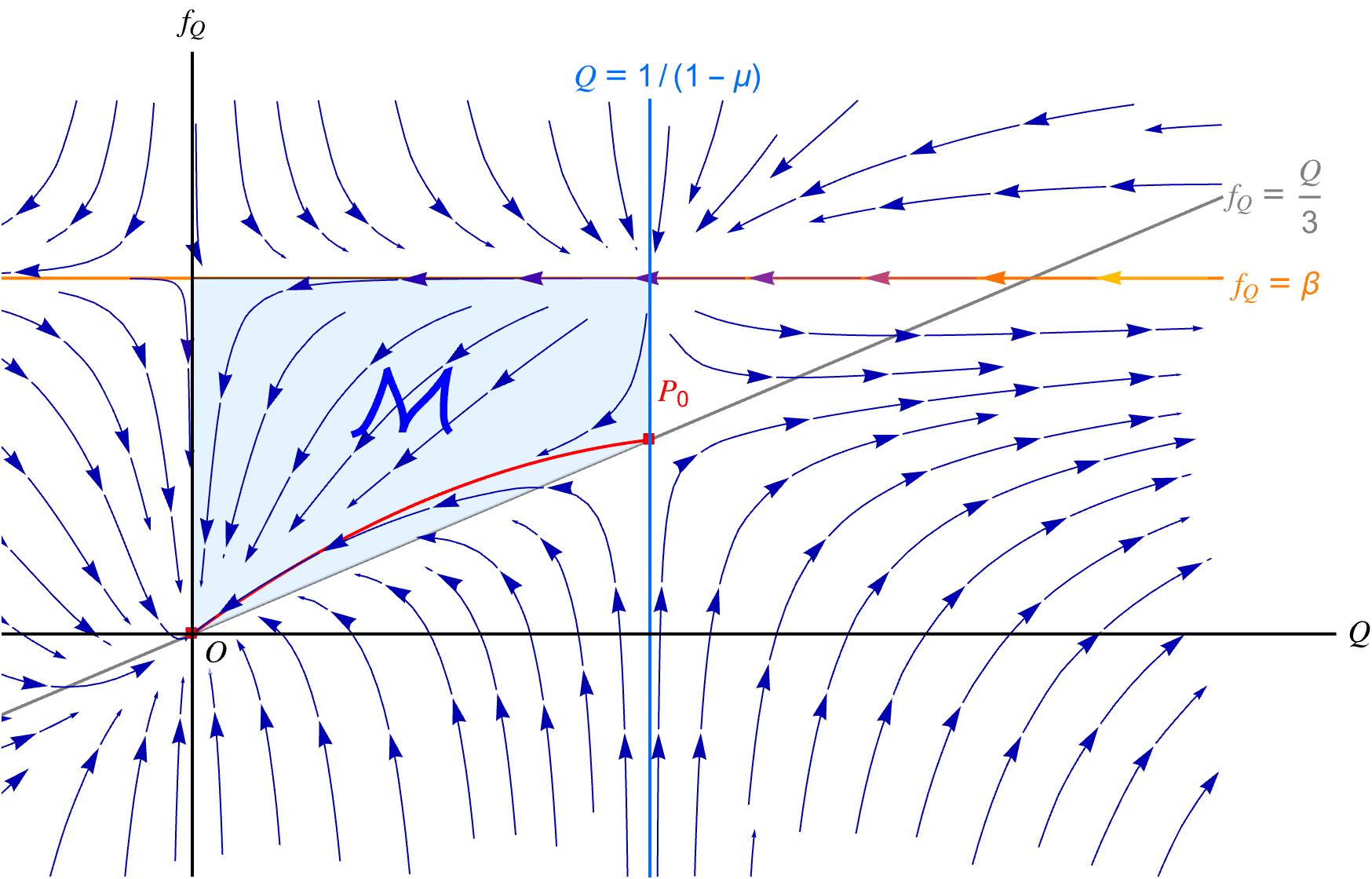
Figure 3. $Qf_{Q}$-plane with $P_{0}$ below $f_{Q}=\beta$. In this case, we can always choose countably many $\{\beta_{j}\}_{j}$ (see Theorem 1.1 and Lemma 3.2 for more details) such that there exists a smooth solution curve (the red curve in the figure) lying in ${\mathcal{M}}$ and connecting $P_{0}$ and the origin $O$ simultaneously, we will discuss this case in more details later in Lemma 3.2.

1.3.3. Stability analysis beyond the spectral theory.

We select the self-similar blowup solution (1.13) of the aggregation equation (1.12) as an approximate solution to (KS-D). We then proceed to study the perturbation dynamics near the profile $Q$ under the self-similar coordinate (4.2), which constitutes the key to our stability analysis.

In the literature, one of the natural approaches to address this problem is to analyze the spectral properties of the associated linearized operator. Such analysis typically relies on compactness arguments [6, 9, 26, 39, 43, 45, 47] or other more intricate operator theory, e.g. studying the precise or approximated spectrum of the linearized operator [18, 34, 44, 49, 53]. For simple problems with an explicit profile available, studying the spectrum of the linearized operator around the profile yields useful information for stability, e.g. [18, 44, 49]. However, for more complicated dynamics with only implicit or numerically approximate profiles, as is our case, obtaining the spectral information becomes significantly more challenging.

Alternatively, we adopt a robust approach based on energy estimates with a singular weight appropriately chosen. Linear stability can be extracted via enforcing local vanishing conditions of the perturbation and singular weights at the origin, using only limited information of the profile. The idea was first demonstrated via the seminal works of [13, 15] in the self-similar case, and later on generalized by the second author with collaborators to type I singularities beyond self-similarity [16, 35] with the blowup law automatically inferred. Such a stability argument via singular weights will be further amenable to computer-assisted proofs. In this paper, we further generalize the idea to the finite-codimensional stability case by studying this open problem.

1.4. Structure of the paper.

In Section 2, we briefly discuss the approach for handling the finite-codimensional stability of blowup solutions to the $1$D semilinear heat equation by introducing the singular weights. Motivated by this illustrative example, we then focus on the Keller-Segel equation with logistic damping term (KS-D). In Section 3, given any fixed $\mu\in\left[0,\frac{1}{3}\right)$, we establish the existence of nontrivial solutions to equation (1.8) with an appropriate choice of $\beta\in\left(\frac{1}{3(1-\mu)},\frac{1}{2}\right)$, the quantitative properties of the approximate profiles will be investigated as well. For the stability analysis, we first examine the coercivity of the linearized operator in the $L_{w}^{2}$ sense with $w$ being sufficiently singular at the origin, as detailed in Section 4. Finally in Section 5, we will study the nonlinear stability to complete the proof of Theorem 1.1.

1.5. Notations.

We denote

$$\left\langle r\right\rangle=\sqrt{1+r^{2}}.$$

And we define a radial smooth cut-off function $\chi$ on $B(0,1)$ by

$$\chi(x)=\begin{cases}1,&\text{if }|y|\leq 1,\\ 0,&\text{if }|y|\geq 2.\end{cases}$$ (1.17)

Based on this, we define the smooth cut-off function on $B(0,R)$ by

$$\chi_{R}(x):=\chi\left(\frac{x}{R}\right).$$ (1.18)

For any given weighted function $w:\mathbb{R}^{3}\to\mathbb{R}$, we define $L_{w}^{2}(\mathbb{R}^{3})$ the weighted inner product by

$$(g_{1},g_{2})_{L_{w}^{2}(\mathbb{R}^{3})}=\int_{\mathbb{R}^{3}}g_{1}(x)g_{2}(x)w(x)dx,$$

and the weighted $L^{2}$ space $L_{w}^{2}(\mathbb{R}^{3})$ by the collections of all functions of $g$ satisfying $\|g\|_{L_{w}^{2}}^{2}:=(g,g)_{L_{w}^{2}}<\infty$.

Furthermore, we define $C_{0}^{\infty}(\Omega)$ as the collection of all $C^{\infty}(\mathbb{R}^{3})$ functions with compact support in $\Omega\subset\mathbb{R}^{3}$.

For any fixed $m\in\mathbb{Z}_{\geq 0}$, we define $\dot{H}^{2m}$ the collection of all functions satisfying

$$\|g\|_{\dot{H}^{2m}}^{2}=\int_{\mathbb{R}^{3}}|\Delta^{m}g|^{2}dx<\infty,$$

and define $\dot{H}^{2m+1}$ the collection of all functions satisfying

$$\|g\|_{\dot{H}^{2m+1}}^{2}=\int_{\mathbb{R}^{3}}|\nabla\Delta^{m}g|^{2}dx<\infty.$$

In addition, we denote $H^{k}(\mathbb{R}^{3})$ for the collection of all functions with finite $\dot{H}^{m}$ norm for all $0\leq m\leq k$. And $H_{rad}^{k}$ is the collection of all radial functions lying in $H^{k}$. Moreover, wewrite $H^{\infty}(\mathbb{R}^{3}):=\cap_{k=0}^{\infty}H^{k}(\mathbb{R}^{3})$.

If $h(x)=h\left(|x|\right)$ is a smooth radial function on $\mathbb{R}^{3}$, then $h(r)$ can be approximated by the Taylor expansion at the origin:

$$h(r)=\sum_{j=0}^{M}[h]_{j}r^{2j}+O(r^{2M+2}),\;\text{ with }\;[h]_{j}:=\frac{\partial_{r}^{(2j)}h}{(2j)!}\Bigg{|}_{r=0},$$ (1.19)

where $[h]_{j}$ is the $2j$-th order coefficient of Taylor expansion of $h(r)$ at the origin.

Acknowledgement.  Jiaqi Liu was supported by NSF grant DMS-2306910, and Yixuan Wang was supported by NSF Grant DMS-2205590. The authors gratefully acknowledge Yao Yao for valuable discussions and insightful suggestions throughout this research. We would like to express our great gratitude to Zhongtian Hu for the informative discussions. Our thanks also extend to Thomas Y. Hou, Juhi Jang, Van Tien Nguyen, Xiang Qin, Jia Shi, and Peicong Song for their valuable suggestions to our work. Finally, we thank the IMS workshop on "Singularities in Fluids and General Relativity" for providing the opportunity for collaboration.

2. Motivating example of 1D semilinear heat equation

In this section, to illustrate the ideas of proof more clearly, we first consider the simpler $1$D semilinear heat equation as a motivating example. Precisely, we will briefly sketch the high-level idea to study high-order vanishing type-I blowup for the $1$D semilinear heat equation under radial (even symmetric) setting:

$$u_{t}=u_{xx}+u^{2}.$$ (HEAT)

2.1. Self-similar renormalization and the approximate solution

For any fixed $m\in\mathbb{Z}_{>1}$, we introduce the self-similar coordinate

$$y=\frac{x}{\lambda^{\frac{1}{m}}},\quad\frac{d\tau}{dt}=\frac{1}{\lambda^{2}},\quad\tau\Big{|}_{t=0}=0,\quad\frac{\lambda_{\tau}}{\lambda}=-\frac{1}{2},$$ (2.1)

and corresponding renormalization

$$u(t,x)=\frac{1}{\lambda^{2}}U\left(\tau,y\right),$$ (2.2)

then $\lambda(\tau)=\lambda_{0}e^{-\frac{1}{2}\tau}$ and $U$ solves the equation

$$\partial_{\tau}U=\lambda^{2-\frac{2}{m}}U_{yy}-U-\frac{1}{2m}y\cdot\nabla U+U^{2},$$ (2.3)

where the diffusion term can be regarded as a perturbation since $2-\frac{2}{m}>0$. This in turn motivates us to find an approximate solution solving the equation

$$-U-\frac{1}{2m}y\cdot\nabla U+U^{2}=0.$$ (2.4)

In particular, this equation can be explicitly solved by

$$U_{*}(y)=(1+cy^{2m})^{-1}.$$ (2.5)

Here $c>0$ is a constant, and $m>1$ describes the vanishing order of the next order expansion of $U_{*}$ near the origin.

2.2. Linear stability

We fix $m>1$ and $c=1$ in (2.5), and plug the ansatz $U=U_{*}+\varepsilon$ into (2.3), it then follows that $\varepsilon$ solves

$$\partial_{\tau}\varepsilon=\lambda^{2-\frac{2}{m}}U_{yy}+{\mathcal{L}}\varepsilon+\varepsilon^{2},$$

where the linearized operator reads

$$\mathcal{L}\varepsilon=-\varepsilon-\frac{1}{2m}y\partial_{y}\varepsilon+2U_{*}\varepsilon.$$ (2.6)

Next, we introduce a weighted $L_{\Theta}^{2}$ space with singular weight $\Theta(y)=y^{-4m-4}$ near the origin to extract damping, which is the essential step to close the nonlinear stability. Via the integration by parts, we have the coercivity near the origin

$$\left({\mathcal{L}}\varepsilon,\varepsilon\right)_{L_{\Theta}^{2}}=\left(\left(-1+2U_{*}+\frac{(\Theta y)_{y}}{4m\Theta}\right)\varepsilon,\varepsilon\right)_{L_{\Theta}^{2}}\approx-\frac{3}{4m}\left(\varepsilon,\varepsilon\right)_{L_{\Theta}^{2}}.$$ (2.7)

In particular, with careful analysis, there is a small constant $0<\kappa=\kappa(m,U_{*})\ll 1$ such that (2.7) can be extended to

$$\left({\mathcal{L}}\varepsilon,\varepsilon\right)_{L_{\Theta+\kappa}^{2}}\leq-\frac{1}{4m}\left(\varepsilon,\varepsilon\right)_{L_{\Theta+\kappa}^{2}}.$$ (2.8)

Additionally, we need to introduce the higher Sobolev norm $\dot{H}^{\bar{K}}$ to close the bootstrap argument. Precisely,

$$\left({\mathcal{L}}\varepsilon,\varepsilon\right)_{\dot{H}^{\bar{K}}} =\left(\left(-1-\frac{\bar{K}}{2m}+2U_{*}+\frac{1}{4m}\right)\partial_{y}^{\bar{K}}\varepsilon,\partial_{y}^{\bar{K}}\varepsilon\right)_{L^{2}}+O(\|\varepsilon\|_{H^{\bar{K}-1}}\|\varepsilon\|_{\dot{H}^{\bar{K}}})$$

$$\leq-\frac{2\bar{K}-4m-1}{4m}\|\varepsilon\|_{\dot{H}^{\bar{K}}}^{2}+O(\|\varepsilon\|_{H^{{\bar{K}}-1}}\|\varepsilon\|_{\dot{H}^{\bar{K}}}),$$ (2.9)

where the leading order enjoys damping once we choose $\bar{K}=\bar{K}(m)\gg 1$.

2.3. Modulation ODEs and nonlinear stability

With the singular weight $\Theta(y)=|y|^{-4m-4}$ given previously, we further radially decompose $\varepsilon$ into

$$\varepsilon(\tau,y)=\varepsilon_{u}(\tau,y)+\varepsilon_{s}(\tau,y),\quad\text{ with }\quad\varepsilon_{u}=\sum_{j=0}^{m}c_{j}(\tau)\chi(y)y^{2j},$$ (2.10)

such that $\varepsilon_{s}(\tau,y)=O(y^{2m+2})$ near the origin, which yields an ODE system for modulation parameters $\{c_{j}\}_{j=0}^{m}$:

$$\begin{cases}\dot{c}_{j}=\left(1-\frac{j}{m}\right)c_{j}+[\varepsilon_{u}^{2}]_{j}+\lambda^{2-\frac{2}{m}}[U_{yy}]_{j},&0\leq j<m-1,\vskip 2.84544pt\\ \dot{c}_{m}=[\varepsilon_{u}^{2}]_{m}-2c_{0}+\lambda^{2-\frac{2}{m}}[U_{yy}]_{m},&j=m.\end{cases}$$ (2.11)

Additionally, $\varepsilon_{s}=O(y^{2m+2})$ solves the equation

$$\partial_{\tau}\varepsilon_{s}=\lambda^{2-\frac{2}{m}}U_{yy}+{\mathcal{L}}\varepsilon_{s}+2\varepsilon_{u}\varepsilon_{s}+\varepsilon_{s}+G[\lambda,U,\varepsilon_{u}],$$

with the modulation term $G[\lambda,U,\varepsilon_{u}]=O(y^{2m+2})$ given by

$$G[\lambda,U,\varepsilon_{u}]=\left(\lambda^{2-\frac{2}{m}}U+{\mathcal{L}}\varepsilon_{u}+\varepsilon_{u}^{2}\right)-\sum_{j=0}^{K}\left[\lambda^{2-\frac{2}{m}}U+{\mathcal{L}}\varepsilon_{u}+\varepsilon_{u}^{2}\right]_{j}\chi y^{2j}.$$

Finally, we can use the standard topological argument together with (2.7) and (2.9) to derive the nonlinear stability with finite codimension $m+1$.

Remark 2.1.

We expect that this nonlinear stability result can be improved to finite-codimension $m-1$, which is two dimensions lower than our previous findings. The key underlying reason is the presence of two degrees of freedom, namely, the choice of the blowup time $T>0$ and the shrinking rate. These degrees of freedom can be utilized through a matching argument to recover the corresponding unstable directions as in [42, 44].

Alternatively, one may employ a method of dynamical rescaling to establish stability at finite codimension $m-1$. Specifically, we modify the coordinate (2.1) as

$$y=\frac{x}{\mu^{\frac{1}{m}}},\quad\frac{d\tau}{dt}=\frac{1}{\lambda^{2}},\quad\tau\big{|}_{t=0}=0,\quad\frac{\lambda_{\tau}}{\lambda}=-\frac{1}{2}+\frac{1}{2}c_{a},\quad\frac{\mu_{\tau}}{\mu}=-\frac{1}{2}-mc_{s}.$$

We then define the corresponding renormalization

$$u(t,x)=\frac{1}{\lambda^{2}}U(\tau,y).$$

Under this coordinate transformation, $U$ satisfies

$$\partial_{\tau}U=\lambda^{2}\mu^{-\frac{2}{m}}U_{yy}+\left(-1+c_{a}\right)U-\left(\frac{1}{2m}+c_{s}\right)y\partial_{y}U+U^{2},$$

where the parameters $(c_{a},c_{s})$ are determined by the modulation conditions

$$U(\tau,0)=U_{*}(0)\qquad\text{ and }\qquad[U(\tau,0)]_{m}=[U_{*}]_{m},$$

and we eliminate neutral modes by fixing $c_{0}=c_{m}=0$. By applying a similar argument of modulation ODEs, we obtain the nonlinear stability with finite codimension $m-1$. Notably, introducing extra scaling parameters to perturb the scaling symmetry is crucial for extending the argument to the nonradial setting; see previous works by the second author and collaborators [16, 35].

Remark 2.2.

Compared with the semilinear heat equation (HEAT), analyzing the Keller-Segel equation with logistic damping (KS-D) involves several additional challenges. For example, the profile $U_{*}$ introduced in (2.5) is an explicit solution to the first-order and separable local equation (2.4). In contrast, for (KS-D) with $\mu\in\left(0,\frac{1}{3}\right)$, the associated profile equation (1.8) is inherently nonlocal and cannot be trivially solved. This nonlocality requires a more delicate analysis, which will be carried out in Section 3.

Moreover, since there is no explicit nontrivial solution to (1.8) with (1.9), additional effort is required to derive quantitative properties of the profile $Q$. Combined with the nonlocal nature of (KS-D), these complexities make the establishment of linear coercivity of Keller-Segel equation more intricate than in the case of the semilinear heat equation (HEAT). Detailed strategies to handle these obstacles will be presented in Section 4.

3. Existence of profile via phase-portrait method

This section is devoted to the existence of smooth profile solving (1.8) when $\mu<\frac{1}{3}$ with the appropriate choices of $\beta$. Firstly, note that for any radially symmetric function $R(y)$ satisfying $R(y)\to 0$ as $|y|\to\infty$,

$$\nabla\Delta^{-1}R(y)=\frac{y}{|y|^{3}}\int_{0}^{|y|}R(s)s^{2}ds,$$ (3.1)

Then, under the radial symmetric assumption, (1.8) becomes

$$\left(\frac{1}{r^{2}}\int_{0}^{r}Q(s)s^{2}ds-\beta r\right)Q^{\prime}(r)-Q+(1-\mu)Q^{2}=0.$$ (3.2)

If $f_{Q}\not=\beta$, by introducing $f_{Q}$ (cf. (1.14)), then we obtain an ODE system of $(Q(r),f(r))$ for $r>0$:

$$\begin{cases}Q^{\prime}(r)=\frac{1}{\beta-f_{Q}}\frac{(1-\mu)Q^{2}-Q}{r},\vskip 5.69046pt\\ f_{Q}^{\prime}(r)=\frac{Q-3f_{Q}}{r}.\end{cases}$$ (3.3)

Remark 3.1.

For notational simplicity, in the subsequent discussion of this section, we introduce the following notations: we write $f:=f_{Q}$, and $Q_{i}:=[Q]_{i}$ and $f_{i}:=[f]_{i}$ for any $i\in\mathbb{Z}_{\geq 0}$, where $f_{Q}$ is given in (3.3), $[Q]_{i}$ and $[f]_{i}$ are the $2i$-th order coefficients of Taylor expansion of $f$ and $Q$ at the origin respectively (cf. (1.19)).

Our main result of this section is as follows, which gives the existence of the nontrivial smooth solutions to (3.3) and the asymptotic behavior of the related solutions when $r=0$ and $r\to\infty$.

Lemma 3.2.

For any fix $\mu\in[0,\frac{1}{3})$, let $\beta:=\beta(j_{0},\mu)=\frac{1}{3(1-\mu)}+\frac{1}{2j_{0}}$ with arbitrarily fixed $j_{0}\geq J>1$ where $J$ is defined in (1.5). Then, for any $Q_{j_{0}}<0$, there exists a unique smooth solution $(Q(r),f(r))$ to (3.3) on $r\geq 0$ with initial conditions:

$$(Q(0),f(0))=\left(\frac{1}{1-\mu},\frac{1}{3(1-\mu)}\right)\quad\text{ and }\quad\partial_{r}^{2j_{0}}Q(0)=(2j_{0})!Q_{j_{0}}.$$ (3.4)

Moreover, the solution $(Q(r),f(r))$ satisfies

1. $(Q(r),f(r))$ is analytic near the origin. Precisely, there exists $\epsilon>0$ such that $(Q(r),f(r))$ can be expressed as Taylor series

   $$Q(r)=\sum_{j=0}^{\infty}Q_{j}r^{2j}\quad\text{and}\quad f(r)=\sum_{j=0}^{\infty}f_{j}r^{2j},\quad\forall\;r\in[0,\epsilon],$$ (3.5)

   where $\{Q_{j}\}_{j\geq 0}$ and $\{f_{j}\}_{j\geq 0}$ satisfy the following recurrence relations

   $$\quad f_{j}=\frac{1}{2j+3}Q_{j},\quad\forall\;j\geq 0,$$ (3.6)

   and

   $$Q_{j}=\begin{cases}\frac{1}{1-\mu},&j=0,\vskip 2.84544pt\\ 0,&0<j<j_{0},\vskip 2.84544pt\\ \frac{\sum_{i=1}^{j-1}\left(\frac{2i}{2(j-i)+3}+(1-\mu)\right)Q_{i}Q_{j-i}}{2j\left(\beta-\frac{1}{2j}-\frac{1}{3(1-\mu)}\right)},&j>j_{0}.\end{cases}$$ (3.7)

2. Both $Q(r),f(r)>0$ are strictly positive for $r\in[0,\infty)$ and monotonically decrease from $Q_{0}=\frac{1}{1-\mu}$ (respectively, $f_{0}=\frac{1}{3(1-\mu)}$) to 0 as $r\to+\infty$.

3. For any $j\geq 0$, there exists a constant $C=C(\beta,Q,j)>0$ such that

   $$|\partial_{r}^{(j)}Q(r)|+|\partial_{r}^{(j)}f(r)|\leq C\left\langle r\right\rangle^{-2-j}\quad\text{for}\quad r\in\overline{\mathbb{R}^{+}}.$$ (3.8)

   In particular, $Q\in H^{\infty}(\mathbb{R}^{3})$.

Proof.

Step 1. Solve (3.3) via Taylor expansion. We assume that $(f(r),Q(r))$ can be expanded into the following forms:

$$f(r)=\sum_{j=0}^{\infty}f_{j}r^{2j},\quad Q(r)=\sum_{j=0}^{\infty}Q_{j}r^{2j},$$

which yields that

$$rf^{\prime}(r)=\sum_{j=0}^{\infty}2jf_{j}r^{2j},\quad rQ^{\prime}(r)=\sum_{j=0}^{\infty}2jQ_{j}r^{2j}.$$

Next, we substitute these expressions into the ODE system (3.3) and match coefficients to establish (3.6) and (3.7). Precisely, we firstly expand the second equation in (3.3) to get that

$$\sum_{j=0}^{\infty}2jf_{j}r^{2j}=\sum_{j=0}^{\infty}\left(Q_{j}-3f_{j}\right)r^{2j}.$$

which directly induces (3.6).

Next, we expand $(\beta-f)r\partial_{r}Q=(1-\mu)Q^{2}-Q$, the first equation in (3.3). Using the identity

$$\left(\sum_{j=0}^{\infty}h_{j}r^{2j}\right)\left(\sum_{j=0}^{\infty}k_{j}r^{2j}\right)=\sum_{j=0}^{\infty}\left(\sum_{i=0}^{j}k_{i}h_{j-i}\right)r^{2j},$$

the left-hand side of the equation becomes

$$\left(\beta-\sum_{j=0}^{\infty}f_{j}r^{2j}\right)\left(\sum_{j=0}^{\infty}2jQ_{j}r^{2j}\right) =\beta\sum_{j=0}^{\infty}2jQ_{j}r^{2j}-\sum_{j=0}^{\infty}\left(\sum_{i=0}^{j}2iQ_{i}f_{j-i}\right)r^{2j}$$

$$=\sum_{j=0}^{\infty}\left(2\beta j-\sum_{i=0}^{j}2iQ_{i}f_{j-i}\right)r^{2j},$$

and the right-hand side of the equation becomes

$$(1-\mu)\sum_{j=0}^{\infty}\left(\sum_{i=0}^{j}Q_{i}Q_{j-i}\right)r^{2j}-\sum_{j=0}^{\infty}Q_{j}r^{2j}=\sum_{j=0}^{\infty}\left((1-\mu)\sum_{i=0}^{j}Q_{i}Q_{j-i}-Q_{j}\right)r^{2j}.$$

Comparing the coefficients onto both sides, we obtain that

$$2\beta jQ_{j}-\sum_{i=0}^{j}2iQ_{i}f_{j-i}=(1-\mu)\sum_{i=0}^{j}Q_{i}Q_{j-i}-Q_{j},\quad\forall\;j\geq 0.$$

Replacing $f_{j-i}$ by using (3.6), we decouple the recurrence relations for $\{Q_{j}\}_{j=0}^{\infty}$ into

$$2\beta jQ_{j}-\sum_{i=0}^{j}\frac{2i}{2(j-i)+3}Q_{i}Q_{j-i}=(1-\mu)\sum_{i=0}^{j}Q_{i}Q_{j-i}-Q_{j},\quad\forall\;j\geq 0.$$

In particular,

$$(1-\mu)Q_{0}^{2}-Q_{0}=0,\quad\text{for }\;j=0,$$

and $Q(0)=Q_{0}=\frac{1}{1-\mu}$ exactly solves this equation. For $j\geq 1$, we isolate the highest index term $Q_{j}$ to obtain

$$2j\Big{(}\beta-\frac{1}{2j}-\frac{1}{3(1-\mu)}\Big{)}Q_{j}=\sum_{i=0}^{j-1}\left(\frac{2i}{2(j-i)+3}+(1-\mu)\right)Q_{i}Q_{j-i}.$$

In particular, applying $j=1$ to the equation together with the fact that $\beta<\frac{1}{2}$ and $1+\frac{1}{3(1-\mu)}>1$, it induces

$$2\left(\beta-\left(\frac{1}{2}+\frac{1}{3(1-\mu)}\right)\right)Q_{1}=0,\quad\Rightarrow\quad Q_{1}=0.$$

Iteratively, with the choice of $\beta=\frac{1}{3(1-\mu)}+\frac{1}{2j_{0}}$,

$$\beta-\frac{1}{2j}-\frac{1}{3(1-\mu)}=\frac{1}{2j_{0}}-\frac{1}{2j}\not=0,\quad\Rightarrow\quad Q_{j}=0,\quad\forall\;2\leq j<j_{0}.$$

Similarly, with $\partial_{r}^{2j_{0}}Q(0)=Q_{j_{0}}<0$ determined in (3.4),

$$\beta-\frac{1}{2j}-\frac{1}{3(1-\mu)}\not=0,\;\Rightarrow\;Q_{j}=\frac{\sum_{i=1}^{j-1}\left(\frac{2i}{2(j-i)+3}+(1-\mu)\right)Q_{i}Q_{j-i}}{2j\left(\beta-\frac{1}{2j}-\frac{1}{3(1-\mu)}\right)},\quad\forall\;j>j_{0}.$$

Hence we obtain the recurrence relation (3.7).

We remark here that under the previous argument, if $\beta-\frac{1}{2j}-\frac{1}{3(1-\mu)}\not=0$ for all $j\geq 1$, then $Q_{j}=0$ for all $j\geq 1$. In this case, $Q(r)\equiv\frac{1}{1-\mu}$, which is a constant solution and not our focus. Hence to obtain a non-constant solution, we must give the vanishing condition that $\beta-\frac{1}{2j_{0}}-\frac{1}{3(1-\mu)}=0$ for some $j_{0}\geq 2$, which exactly matches the choice of $\beta$.

Step 2. Analyticity of $(Q,f)$ near the origin. First of all, recalling [29, Lemma B.1], there exists a universal constant $a>0$ such that for all $L\in\mathbb{N}$,

$$\sum_{\begin{subarray}{c}i+j=L\\ i,j>0\end{subarray}}\frac{1}{i^{2}j^{2}}\leq\frac{a}{L^{2}},$$ (3.9)

which, by using the fact that $Lj\geq i$ for any $1\leq i,j\leq L-1$, yields that

$$\sum_{\begin{subarray}{c}i+j=L\\ i,j>0\end{subarray}}\frac{1}{ij^{3}}\leq\sum_{\begin{subarray}{c}i+j=L\\ i,j>0\end{subarray}}\frac{L}{i^{2}j^{2}}\leq\frac{a}{L}.$$ (3.10)

Next, we are devoted to the estimates of coefficients of the Taylor expansion determined in (3.7). Precisely, we claim that there exists $K,\alpha>0$, such that

$$|Q_{j}|\leq\frac{K^{j-\alpha}}{j^{2}},\quad\forall\;j\geq j_{0},$$ (3.11)

where $K,\alpha>0$ satisfy

$$|Q_{j_{0}}|\leq\frac{K^{j_{0}-\alpha}}{j_{0}^{2}}\quad\text{ and }\quad\frac{aK^{-\alpha}}{\frac{1}{2j_{0}}-\frac{1}{2(j_{0}+1)}}<\frac{1}{2}.$$ (3.12)

In fact, we proceed by induction. For $1\leq j\leq j_{0}$, it automatically holds with (3.7) and (3.12). We now assume that (3.11) holds for any $j_{0}\leq j\leq L$, then by using (3.7), (3.9), (3.10), (3.11) and (3.12), we obtain

$$Q_{L+1} =\frac{1}{2(L+1)\left(\beta-\frac{1}{2(L+1)}-\frac{1}{3(1-\mu)}\right)}\sum_{\begin{subarray}{c}i+j=L+1\\ i,j>0\end{subarray}}\left(\frac{2i}{2j+3}+(1-\mu)\right)Q_{i}Q_{j}$$

$$\leq\frac{1}{2(L+1)\left(\frac{1}{2j_{0}}-\frac{1}{2(j_{0}+1)}\right)}\sum_{\begin{subarray}{c}i+j=L+1\\ i,j>0\end{subarray}}\left(\frac{2i}{2j+3}+(1-\mu)\right)\frac{K^{L+1-2\alpha}}{i^{2}j^{2}}$$

$$\leq\frac{K^{L+1-2\alpha}}{2(L+1)\left(\frac{1}{2j_{0}}-\frac{1}{2(j_{0}+1)}\right)}\sum_{\begin{subarray}{c}i+j=L+1\\ i,j>0\end{subarray}}\left(\frac{1}{ij^{3}}+\frac{1}{i^{2}j^{2}}\right)\leq\frac{K^{L+1-\alpha}}{(L+1)^{2}},$$

which yields the validity of (3.11) with $j=L+1$, hence we have closed the induction and verified the claim.

The analyticity of $Q$ at the origin then follows from Cauchy’s convergence criterion for power series. Precisely, there exists $\epsilon=\epsilon(K)\ll 1$ such that the series

$$Q(r)=\sum_{j=0}^{\infty}Q_{j}r^{2j},\quad\text{ with }Q_{j}\text{ determined in \eqref{recurrence Qj},}$$

is absolutely convergent on $[0,\epsilon]$. The analyticity of $f(r)=\sum_{j=0}^{\infty}f_{j}r^{2j}$ on $r\in[0,\epsilon]$ simply follows (3.6) and the analyticity on $[0,\epsilon]$ of $Q$.

Step 3. Extend $(Q,f)$ to $[0,+\infty)$. At this stage, our objective is to extend the previously constructed solution to $\overline{\mathbb{R}^{+}}$, and verify that both $f(r)$ and $Q(r)$ will asymptotically decay to $0$ and the solution curve (see the red curve in Figure 3)) remains within ${\mathcal{M}}$ with

$$\mathcal{M}:=\left\{(Q,f)\Big{|}\;0<Q<Q_{0},\;\frac{Q}{3}<f<\beta\right\}.$$

Here, recalling (3.3) or Figure 3, we observe that both $(Q(r)$ and $f(r))$ are strictly decreasing once the solution curve stays within ${\mathcal{M}}$, i.e.

$$Q^{\prime}(r)<0,f^{\prime}(r)<0\quad\text{ if}\quad(Q(r),f(r))\in\text{ $\mathcal{M}$}.$$ (3.13)

We first claim that there exists $\nu\in(0,\epsilon)$ such that $(Q(r),f(r))\in{\mathcal{M}},\;\forall\;r\in(0,\nu]$. To verify this, since

$$\frac{d^{j}}{dr^{j}}Q(0)=0,\quad\forall\;1\leq j<2j_{0}\qquad\text{ and }\qquad\frac{d^{2j_{0}}}{dr^{2j_{0}}}Q(0)=(2j_{0})!Q_{j_{0}}<0,$$

it follows that both $Q(r)$ and $f(r)$ are strictly decreasing on $[0,\nu]$ for some $0<\nu\leq\epsilon\ll 1$. Consequently, the portion of the solution curve for $r\in[0,\nu]$, which begins at $P_{0}$ (1.15), remains within the lower-left area of $P_{0}$. Furthermore, it continues to be representable as a graph, meaning that there is a smooth function ${\mathcal{F}}$ with

$$f={\mathcal{F}}(Q)\quad\text{ on }\quad Q\in\left[Q_{0}-\nu_{Q},Q_{0}\right],$$

for some $0<\nu_{Q}\ll 1$. By chain rule, (3.3), (3.5), (3.6) (3.7) and $j_{0}\geq J>1$,

$$\mathcal{F}^{\prime}(Q_{0}) =\frac{df}{dQ}\Big{|}_{(Q,f)=P_{0}}=\lim_{r\to 0^{+}}\frac{(Q(r)-3f(r))(\beta-f(r))}{(1-\mu)Q^{2}(r)-Q(r)}$$

$$=\frac{\beta-f_{0}}{(1-\mu)Q_{0}}\frac{Q_{j_{0}}-3f_{j_{0}}}{Q_{j_{0}}}=\frac{1}{2j_{0}}\left(1-\frac{3}{2j_{0}+3}\right)<\frac{1}{2j_{0}}\leq\frac{1}{4}<\frac{1}{3}.$$

Thus, the slope of the solution curve at $P_{0}$ is strictly less than that of the line $f=\frac{1}{3}Q$, which contains the lower boundary of ${\mathcal{M}}$. So by adjusting $0<\nu\ll 1$ if necessary and using the smoothness of ${\mathcal{F}}$, we conclude that the curve $\{(Q(r),f(r))\}_{r\in(0,\nu]}$ lies above $f=\frac{1}{3}Q$. This has verified the claim.

Next, we prove that the solution curve remains in $\mathcal{M}$ for all $r\in(0,\infty)$. In fact, ensured by the Cauchy-Lipschitz theory, with the strict decay property of the solution within ${\mathcal{M}}$ (see (3.13)), there are only three possible scenarios:

1. there exists $r_{E1}\in(0,\infty]$, such that the solution exits the region $\mathcal{M}$ at a point $\left(Q_{E1},\frac{Q_{E1}}{3}\right)$ through the line $f=\frac{Q}{3}$, where $Q_{E1}=Q(r_{E1})\in\left(0,Q_{0}\right)$;

2. there exists $r_{E2}\in(0,\infty]$, such that the solution exits the region $\mathcal{M}$ at a point $(0,f_{E2})$ through the $f$-axis, where $f_{E2}=f(r_{E2})\in(0,f_{0})$;

3. the solution escapes $\mathcal{M}$ at the origin $O$.

We now eliminate scenarios $(1)$ and $(2)$ by contradiction arguments.

For the scenario $(1)$, we assume that it occurs. Since $(Q(r),f(r))$ is strictly decreasing before reaching the line $f=\frac{Q}{3}$, together with Cauchy-Lipschitz theory, the solution curve can be further extended on $Q\in[Q_{E1},Q_{0}]$ and represented as $Q\mapsto{\mathcal{F}}(Q)$ with ${\mathcal{F}}$ a smooth function.

On the one hand, since $\{(Q(r),f(r))\}_{r\in(0,r_{E_{1}})}\subset{\mathcal{M}}$, it follows that $f(r)>\frac{1}{3}Q(r)$ for any $r\in(0,r_{E_{1}})$ and $f(r),Q(r)$ is strictly decreasing on $r\in(0,r_{E_{1}})$, thus together with $f(r_{E_{1}})=\frac{1}{3}Q(r_{E_{1}})$,

$${\mathcal{F}}^{\prime}(Q_{E1})=\lim_{r\to r_{E_{1}}^{-}}\frac{f(r)-f(r_{E_{1}})}{Q(r)-Q(r_{E_{1}})}\geq\lim_{r\to r_{E_{1}}^{-}}\frac{\frac{1}{3}Q(r)-\frac{1}{3}Q(r_{E_{1}})}{Q(r)-Q(r_{E_{1}})}=\frac{1}{3}.$$

On the other hand, recalling the ODE system (3.3) together with $f(r_{E_{1}})=\frac{1}{3}Q(r_{E_{1}})$ again, we compute

$$\mathcal{F}^{\prime}(Q_{E1})=\lim_{r\to r_{E1}^{-}}\frac{(Q(r)-3f(r))(\beta-f(r))}{(1-\mu)Q^{2}(r)-Q(r)}=0<\frac{1}{3},$$

which contradicts our assumption and hence we have ruled out the scenarios $(1)$.

Regarding the second scenario $(2)$, by an argument analogous to that of the first case, the solution curve can be extended on $f\in[f_{E2},f_{0}]$ and represented as $f\mapsto{\mathcal{Q}}(f)$ with ${\mathcal{Q}}$ a smooth function, and thus

$$\{\left(Q(r),f(r)\right)\}_{r\in\big{(}0,r_{E_{2}}\big{)}}=\{\left({\mathcal{Q}}(f),f\right)\}_{f\in\big{(}f_{E_{2}},f_{0}\big{)}}\subset{\mathcal{M}}.$$ (3.14)

Recall (3.3) again, ${\mathcal{Q}}(f)$ is governed by the equation

$${\mathcal{Q}}^{\prime}=\frac{(1-\mu){\mathcal{Q}}^{2}-{\mathcal{Q}}}{({\mathcal{Q}}-3f)(\beta-f)},\quad\forall\;f\in[f_{E2},f_{0}],$$ (3.15)

whose local wellposedness near $f=f_{E_{2}}$ is well established by the Cauchy-Lipschitz theory. Nevertheless, besides the nontrivial solution curve given in (3.14), we observe that $\{(0,f)\}_{f\in[f_{E_{2}},f_{0}]}$ is also a satisfied solution curve, which leads to a contradiction and hence we have ruled out the scenario $(2)$.

Consequently, we have shown that the solution curve could only exist $\mathcal{M}$ at the origin $O$, i.e. in scenario $(3)$. To conclude this step, it suffices to verify that

$$\lim_{r\to\infty}(Q(r),f(r))=(0,0).$$ (3.16)

In fact, similar to the previous argument, the solution curve can be further smoothly extended and represented as $Q\mapsto{\mathcal{F}}(Q)$ on $[0,Q_{0}]$. Additionally, using (3.13) again, the function $r\mapsto Q(r)$ is one-to-one and thus $r$ can be expressed by $r={\mathcal{R}}(Q)$ on $Q\in[0,Q_{0}]$, with ${\mathcal{R}}$ solving

$$\mathcal{R}^{\prime}(Q)=\mathcal{R}(Q)\frac{\beta-\mathcal{F}(Q)}{(1-\mu)Q^{2}-Q},$$

which follows from the inverse function theorem and (3.3). Then, a direct computation together with (3.4), (3.6), (3.13) and the fact that $\mathcal{R}(\frac{Q_{0}}{2})\in(0,\infty)$ yields that

$$\lim_{Q\to 0^{+}}\ln\mathcal{R}(Q) =\ln\mathcal{R}\left(\frac{Q_{0}}{2}\right)+\lim_{Q\to 0^{+}}\int_{\frac{Q_{0}}{2}}^{Q}\frac{\beta-\mathcal{F}(\tilde{Q})}{(1-\mu)\tilde{Q}^{2}-\tilde{Q}}\ d\tilde{Q}$$

$$>\ln\mathcal{R}\left(\frac{Q_{0}}{2}\right)+(\beta-f_{0})\lim_{Q\to 0+}\int_{\frac{Q_{0}}{2}}^{Q}\left(\frac{1}{\tilde{Q}-\frac{1}{1-\mu}}-\frac{1}{\tilde{Q}}\right)\ d\tilde{Q}=+\infty,$$

hence we have verified (3.16) and finished this step.

Step 4. Uniqueness. Assume that there exists two smooth solution $(Q^{(1)},f^{(1)})$ and $(Q^{(2)},f^{(2)})$ solving the system (3.3) with the same initial conditions (3.4), then by the $C^{\infty}$ continuity of $Q$ at the origin and a similar argument as in Step 1 and Step 3, it can be verified that $(Q^{(i)},f^{(i)})$ satisfies

$$Q_{0}^{(1)}=Q_{0}^{(2)}=\frac{1}{1-\mu},\quad Q_{j}^{(1)}=Q_{j}^{(2)}=0\quad\left(\text{with }1\leq j<j_{0}-1\right),\quad Q_{j_{0}}^{(1)}=Q_{j_{0}}^{(2)}<0,$$ (3.17)

and both $Q^{(i)}(r)$ and $f^{(i)}(r)$ are strictly decreasing on $\mathbb{R}^{+}$ for both $i=1,2$. Next, we study the difference between these two solutions. Denote

$$(\triangle Q,\triangle f):=(Q^{(1)}-Q^{(2)},f^{(1)}-f^{(2)}),$$

which solves the following ODE system:

$$\begin{cases}(\triangle Q)^{\prime}=\frac{1}{\beta-f^{(1)}}\frac{(1-\mu)(Q^{(1)}+Q^{(2)})\triangle Q-\triangle Q}{r}-\frac{(1-\mu)(Q^{(2)})^{2}-Q^{(2)}}{r}\frac{\triangle f}{(\beta-f^{(1)})(\beta-f^{(2)})},\vskip 2.84544pt\\ (\triangle f)^{\prime}=\frac{\triangle Q-3\triangle f}{r}.\end{cases}$$

We define

$${\mathcal{E}}(r):=|\triangle Q(r)|^{2}+|\triangle f(r)|^{2},$$

and compute

$$\;\;{\mathcal{E}}^{\prime} =I+II,$$

$$\text{ with }\ \ I =2\frac{\triangle f\triangle Q-3(\triangle f)^{2}}{r}+2\frac{(1-\mu)(Q^{(1)}+Q^{(2)})-1}{(\beta-f^{(1)})r}(\triangle Q)^{2},$$

$$\;II =-2\frac{(1-\mu)(Q^{(2)})^{2}-Q^{(2)}}{r}\frac{1}{(\beta-f^{(2)})(\beta-f^{(1)})}\triangle f\triangle Q,$$

By using Cauchy inequality, strictly decreasing fact of $Q^{(i)}(r)$ and $f^{(i)}(r)$, (3.4) and (3.6), we bound $I$ by

$$I\leq\Big{(}1+2\frac{(1-\mu)(Q^{(1)}(0)+Q^{(2)}(0))-1}{(\beta-f^{(1)}(0))}\Big{)}\frac{\mathcal{E}(r)}{r}=(4j_{0}+1)\frac{\mathcal{E}(r)}{r}.$$

Applying condition (3.17) along with the Cauchy’s inequality, there exists constant $M=M(j_{0},\mu,Q^{(1)},Q^{(2)})>0$ such that

$$II\leq M|\triangle f\triangle Q|\leq M{\mathcal{E}}(r),$$

which yields that

$${\mathcal{E}}^{\prime}(r)=I+II\leq(4j_{0}+1)\frac{{\mathcal{E}}(r)}{r}+M{\mathcal{E}}(r).$$

Applying Gronwall’s inequality,

$$0\leq{\mathcal{E}}(r)\leq{\mathcal{E}}(\delta)\left(\frac{r}{\delta}\right)^{4j_{0}+1}e^{M(r-\delta)},\quad\text{ uniformly for }r,\delta>0.$$

Since $(Q^{(i)},f^{(i)})$ (with $i=1,2$) satisfy the same initial conditions (3.17), it follows that

$$\partial_{r}^{j}{\mathcal{E}}(r)\Big{|}_{r=0}=0,\quad\forall\;0\leq j\leq 4j_{0}+2,$$

which implies that

$$\lim_{\delta\to 0+}\frac{{\mathcal{E}}(\delta)}{\delta^{4j_{0}+1}}e^{-M\delta}=0.$$

By the squeezing theorem, it follows that ${\mathcal{E}}(r)\equiv 0$ for any $r\geq 0$. Consequently, we conclude $Q^{(1)}\equiv Q^{(2)}$ and this completes the uniqueness.

Step 5. Decay estimate of $Q$ and its derivative. Based on the discussion in Step 3, both $Q(r)\searrow 0$ and $f(r)\searrow 0$ as $r\to\infty$. Next for any fixed $\nu_{0}>0$, recalling the choice of $\beta=f_{0}+\frac{1}{2j_{0}}$, there exists $M_{0}=M_{0}(\nu_{0})\gg 1$ such that

$$\qquad\quad 0<(1-\nu_{0})Q(r)\leq Q(r)-(1-\mu)Q^{2}(r)\leq Q(r),\quad\forall\;r\geq M_{0},$$

$$\text{ and }\;\;-2j_{0}\leq-\frac{1}{\beta-f}\leq-\frac{1}{\beta}<0.$$

From the ODE (3.3) satisfied by $Q(r)$, these inequalities imply

$$-\frac{2j_{0}Q}{r}\leq Q^{\prime}(r)\leq-\frac{(1-\nu_{0})Q}{\beta r},\quad\quad\forall\;r\geq M_{0},$$

hence

$$Q(r)\leq Q(M_{0})\left(\frac{r}{M_{0}}\right)^{-\frac{1}{\beta}(1-\nu_{0})},\quad\forall\;r\geq M_{0}.$$

In particular, since $\beta<\frac{1}{2}$, we can choose $\nu_{0}>0$ sufficiently small such that $\frac{1-\nu_{0}}{\beta}<2$. This allows us to find a constant $C=C(\beta,M_{0})>0$ such that

$$Q(r)\leq C\left\langle r\right\rangle^{-2},\quad\forall\;r\geq 0.$$ (3.18)

Moreover, using the second equation in (3.3), there exists a constant $C=C(\beta,M_{0})>0$ such that

$$0<f(r)=\frac{1}{r^{3}}\int_{0}^{r}Q(s)s^{2}ds\leq\frac{C}{r^{3}}\int_{0}^{r}\frac{s^{2}}{\left\langle s\right\rangle^{2}}ds\leq C\left\langle r\right\rangle^{-2},\quad\forall\;r\geq 0.$$ (3.19)

For the derivatives of $Q(r)$ and $f(r)$, applying $\partial_{r}^{j-1}$ (with $j\geq 1$) to (3.3) and using the base decay estimates (3.18) and (3.19), a straightforward induction then shows that

$$|\partial_{r}^{(j)}Q(r)|\leq C\left\langle r\right\rangle^{-2-j},$$ (3.20)

for some constant $C=C(\beta,M_{0},j)>0$.

Finally, combining the $C^{\infty}$ smoothness of $Q$, the above decay bound on $\partial_{r}^{(j)}Q$ (cf. (3.18) and (3.20)), and the standard identity $Dg=\frac{x}{|x|}\cdot\nabla g$ for radial function $g$, we can verify that $Q\in H^{\infty}(\mathbb{R}^{3})$. This completes the proof of the lemma. ∎

Based on Lemma 3.2, one naturally obtains the existence of a smooth profile satisfying (1.8). More precisely, we have the following result.

Corollary 3.3 (Existence of smooth self similar profile).

Under the assumptions of Lemma 3.2, for any fixed $[Q]_{j_{0}}<0$, there exists a unique smooth radial symmetric solution $Q\in H^{\infty}(\mathbb{R}^{3})$ to (1.8) satisfying

$$Q(0)=\frac{1}{1-\mu},\quad\text{ and }\partial_{r}^{(2j_{0})}Q(0)=(2j_{0})![Q]_{j_{0}}<0.$$ (3.21)

In particular, $Q(r)$ is strictly radially decreasing with respect to $r\geq 0$ and satisfies the decay estimates (3.8).

4. Linear theory

Starting from this section, we fix $\mu\in[0,\frac{1}{3})$ and a positive integer $j_{0}\geq\frac{3(1-\mu)}{1-3\mu}+1>1$, then we have

$$\beta=\frac{1}{3(1-\mu)}+\frac{1}{2j_{0}}\in\left(0,\frac{1}{2}\right).$$ (4.1)

We now introduce the self-similar coordinate:

$$y=\frac{x}{\lambda^{2\beta}},\quad\frac{d\tau}{dt}=\frac{1}{\lambda^{2}},\quad\tau\Big{|}_{t=0}=0,\quad\frac{\lambda_{\tau}}{\lambda}=-\frac{1}{2},$$ (4.2)

and the corresponding renormalization

$$\rho(t,x)=\frac{1}{\lambda^{2}}\Psi\left(\tau,y\right).$$ (4.3)

The equation (KS-D) can be mapped into the renormalization system of $\Psi$:

$$\partial_{\tau}\Psi=\lambda^{2-4\beta}\Delta\Psi-\Psi-\beta y\cdot\nabla\Psi+\nabla\Psi\cdot\nabla\Delta^{-1}\Psi+(1-\mu)\Psi^{2},$$ (4.4)

where, from (4.2), the function $\lambda$ is

$$\lambda(\tau)=\lambda_{0}e^{-\frac{1}{2}\tau},\quad\forall\;\tau\geq 0,$$ (4.5)

with initial data given by $\lambda\Big{|}_{\tau=0}=\lambda_{0}>0$.

Next, we consider a solution to above equation in perturbative form

$$\Psi=Q+\varepsilon,$$

where $Q$ is a solution to the PDE (1.8), corresponding to the fixed parameters $\mu$ and $j_{0}$, whose existence is established in Lemma 3.2. Direct computation shows the residue $\varepsilon$ solves

$$\partial_{\tau}\varepsilon={\mathcal{L}}\varepsilon+\lambda^{2-4\beta}\Delta\Psi+N(\varepsilon),$$ (4.6)

where ${\mathcal{L}}$ is the linear operator

$${\mathcal{L}}\varepsilon=-(\varepsilon+\beta y\cdot\nabla\varepsilon)+\nabla\varepsilon\cdot\nabla\Delta^{-1}Q+\nabla Q\cdot\nabla\Delta^{-1}\varepsilon+2(1-\mu)Q\varepsilon,$$ (4.7)

and $N(\varepsilon)$ is the nonlinear term

$$N(\varepsilon)=\nabla\varepsilon\cdot\nabla\Delta^{-1}\varepsilon+(1-\mu)\varepsilon^{2}.$$ (4.8)

For the linear operator ${\mathcal{L}}$ given in (4.7), we will prove its coercivity in the sense of $L_{w}^{2}$ for some weight $w$ sufficiently singular at the origin. Precisely, we have the following result:

Proposition 4.1 (Coercivity of ${\mathcal{L}}$ in $L_{w}^{2}$).

For ${\mathcal{L}}$ given in (4.7), there exists a weight defined by

$$w(y):=|y|^{-A}+B,$$ (4.9)

where $(A,B)\in\mathbb{Z}_{+}\times\mathbb{R}_{+}$ satisfy $A\gg 4j_{0}+3$ and $\frac{A}{4}\in\mathbb{Z}_{>0}$, such that ${\mathcal{L}}$ satisfies the coercivity in the following sense:

$$\left({\mathcal{L}}g,g\right)_{L_{w}^{2}}\leq-\frac{1}{8}\|g\|_{L_{w}^{2}}^{2},\quad\forall\;g\in L_{w}^{2}(\mathbb{R}^{3}).$$ (4.10)

Remark 4.2.

Due to the limited quantitative properties of $Q$ available from Lemma 3.2 and the nonlocal structure of the operator $\mathcal{L}$, it is difficult to identify the optimal value of $A$ explicitly, in contrast with the situation for the heat equation discussed in Section 2. Nevertheless, the existence of some $A$ satisfying (4.10) is sufficient for our subsequent analysis.

Proof of Proposition 4.1.

First of all, for any $g\in L_{w}^{2}$, by integration by parts, (3.1) and the fact that $y\cdot\nabla w=-A|y|^{-A}$,

$$-\beta\int(y\cdot\nabla g)gwdy=\frac{\beta}{2}\left(-A+3\right)\int g^{2}|y|^{-A}dy+\frac{3B\beta}{2}\int g^{2}dy,$$

and

$$\int\left(\nabla g\cdot\nabla\Delta^{-1}Q\right)gwdy=-\frac{1}{2}\int Qg^{2}wdy+\frac{A}{2}\int g^{2}f_{Q}|y|^{-A}dy,$$ (4.11)

with which, recalling the definition of ${\mathcal{L}}$ ( see (4.7)), we split $({\mathcal{L}}g,g)_{L_{w}^{2}}$ into the following three parts:

$$({\mathcal{L}}g,g)_{L_{w}^{2}}=I_{SI}+I_{LO}+I_{NLO},$$ (4.12)

where

$$I_{SI}:=\left(-1+\frac{\beta}{2}(-A+3)\right)\int g^{2}|y|^{-A}dy+\frac{A}{2}\int g^{2}f_{Q}|y|^{-A}dy+\left(\frac{3}{2}-2\mu\right)\int g^{2}Q|y|^{-A}dy,$$

$$I_{LO}:=\left(-B+\frac{3B\beta}{2}\right)\int g^{2}dy+\left(\frac{3}{2}-2\mu\right)B\int g^{2}Qdy,\quad I_{NLO}:=\int\left(\nabla Q\cdot\nabla\Delta^{-1}g\right)gwdy.$$

Here $I_{SI}$ denotes the sum of local terms involving the singular weight $|y|^{-A}$, $I_{LO}$ denotes the sum of local terms without singular weight, and $I_{NLO}$ denotes the sum of nonlocal terms.

Estimate of $I_{SI}$. By Lemma 3.2, $Q$ and $f_{Q}$ are both radially decreasing. Moreover, recalling the initial conditions of $(Q(0),f_{Q}(0))$ given in (3.4) and the definition of $\beta$ in (4.1), $I_{SI}$ can be estimated by

$$I_{SI} \leq\left(-1+\frac{\beta}{2}(-A+3)\right)\int g^{2}|y|^{-A}dy+\left(\frac{A}{2}f_{Q}(0)+\left(\frac{3}{2}-2\mu\right)Q(0)\right)\int g^{2}|y|^{-A}dy$$

$$=\left(-1+\frac{\frac{1}{3(1-\mu)}+\frac{1}{2j_{0}}}{2}(-A+3)+\frac{A}{6(1-\mu)}+\left(\frac{3}{2}-2\mu\right)\frac{1}{1-\mu}\right)\int g^{2}|y|^{-A}dy$$

$$=\left(1+\frac{-A+3}{4j_{0}}\right)\int g^{2}|y|^{-A}dy,$$ (4.13)

where the coercivity becomes significantly stronger as $A\gg 1$ grows.

We remark here that the derivation of (4.13) is rather delicate. Precisely, one might naturally expect that the term $g+\beta y\cdot\nabla g$ alone provides enhanced coercivity with increasing $A$. However, this gain is offset by the contribution $\frac{A}{2}\int g^{2}f_{Q}|y|^{-A}dy$, which greatly diminishes the coercivity originating from the scaling term. Nevertheless, with the estimate given in (4.13), we find that this essential obstacle can be almost exactly controlled via the fact that $\beta-f_{Q}(r)\geq\beta-f_{Q}(0)=\frac{1}{2j_{0}}>0$.

Estimate of $I_{LO}$. Again, by Lemma 3.2, $Q$ is radially decreasing and $\Big{\|}|y|^{-\frac{1}{2}}\partial_{r}Q\Big{\|}_{L^{2}}<\infty$, so there exists $R_{1}=R_{1}(Q)\gg 1$ such that

$$\frac{3}{2}Q(R_{1})\leq\frac{1}{1000}\quad\text{ and }\quad\Big{\|}|y|^{-\frac{1}{2}}\partial_{r}Q\Big{\|}_{L^{2}(|x|\geq R_{1})}\leq\frac{1}{5000}.$$ (4.14)

Noting that $\beta<\frac{1}{2}$, we may now estimate the lower-order term $I_{LO}$ as follows:

$$I_{LO} \leq\left(-B+\frac{3}{4}B\right)\int g^{2}dy+\left(\frac{3}{2}-2\mu\right)B\left(\int_{|y|\leq R_{1}}g^{2}Qdy+\int_{|y|\geq R_{1}}g^{2}Qdy\right)$$

$$\leq-\frac{B}{4}\int g^{2}dy+\left(\frac{3}{2}-2\mu\right)BQ(0)R_{1}^{A}\int_{|y|\leq R_{1}}g^{2}|y|^{-A}dy+\left(\frac{3}{2}-2\mu\right)BQ(R_{1})\|g\|_{L^{2}}^{2}$$

$$=-\frac{3B}{16}\|g\|_{L^{2}}^{2}+\left(\frac{3}{2}-2\mu\right)BQ(0)R_{1}^{A}\|g\|_{L_{|y|^{-A}}^{2}}^{2}.$$ (4.15)

Given the limited qualitative information about $Q$, the term involving $Q$ cannot be directly controlled, especially the integral of $\int_{|y|\leq R_{1}}\int g^{2}Qdy$, where $Q(y)=O(1)$ on $B(0,R_{1})$. To address this, we absorb this term using the previous coercivity (4.13) by choosing $0<B\ll 1$ sufficiently small.

Estimate of $I_{NLO}$. By Cauchy’s inequality, the nonlocal term involving in $I_{NLO}$ can be controlled pointwise by

$$\quad\frac{1}{r^{2}}\int_{0}^{r}|g(s)|s^{2}ds=\frac{1}{4\pi r^{2}}\int_{B(0,r)}|g(y)|dy=\frac{1}{4\pi r^{2}}\int_{B(0,r)}|g(y)||y|^{-\frac{A}{2}}|y|^{\frac{A}{2}}dy$$

$$\leq\frac{1}{4\pi r^{2}}\left(\int_{B(0,r)}g^{2}(y)|y|^{-A}dy\right)^{\frac{1}{2}}\left(\int_{B(0,r)}|y|^{A}dy\right)^{\frac{1}{2}}=\sqrt{\frac{1}{4\pi(A+3)}}r^{\frac{A}{2}-\frac{1}{2}}\|g\|_{L_{|y|^{-A}}^{2}},$$ (4.16)

and this induces that

$$\quad\Bigg{|}\int\left(\nabla Q\cdot\nabla\Delta^{-1}g\right)g|y|^{-A}dy\Bigg{|}=\int|\partial_{r}Q|\left(\frac{1}{|y|^{2}}\int_{0}^{|y|}|g(s)|s^{2}ds\right)|g||y|^{-A}dy$$

$$\leq\sqrt{\frac{1}{4\pi(A+3)}}\|g\|_{L_{|y|^{-A}}^{2}}\int|\partial_{r}Q||g||y|^{-\frac{A}{2}-\frac{1}{2}}dy\leq\sqrt{\frac{1}{4\pi(A+3)}}\Big{\|}|y|^{-\frac{1}{2}}\partial_{r}Q\Big{\|}_{L^{2}}\|g\|_{L_{|y|^{-A}}^{2}}^{2},$$ (4.17)

which, by choosing $A\gg 1$ sufficiently large, can be absorbed in (4.13). Similarly, repeating the previous argument, together with the choice of $R_{1}\gg 1$ (see (4.14)), the $L^{2}$ component of $I_{NLO}$ can be controlled by:

$$\quad B\int\left(\nabla Q\cdot\nabla\Delta^{-1}g\right)gdy\leq B\|g\|_{L^{2}}\left(\int_{|y|\leq R_{1}}|\partial_{r}Q||y|^{-\frac{1}{2}}|g|dy+\int_{|y|\geq R_{1}}|\partial_{r}Q||y|^{-\frac{1}{2}}|g|dy\right)$$

$$\leq\frac{B}{100}\|g\|_{L^{2}}^{2}+50BR_{1}^{A}\big{\|}\partial_{r}Q|y|^{-\frac{1}{2}}\big{\|}_{L^{2}}^{2}\|g\|_{L_{|y|^{-A}}^{2}}^{2}+50B\big{\|}\partial_{r}Q|y|^{-\frac{1}{2}}\big{\|}_{L^{2}(|y|\geq R_{1})}^{2}\|g\|_{L^{2}}^{2}$$

$$\leq\frac{B}{50}\|g\|_{L^{2}}^{2}+50BR_{1}^{A}\big{\|}\partial_{r}Q|y|^{-\frac{1}{2}}\big{\|}_{L^{2}}^{2}\|g\|_{L_{|y|^{-A}}^{2}}^{2}.$$ (4.18)

The idea of handling this term is similar to $I_{LO}$, and we can use the smallness of $0<B\ll 1$ to absorb $B\int_{|y|\leq R_{1}}\left(\nabla Q\cdot\nabla\Delta^{-1}g\right)gdy$ by the coercivity (4.13). Hence combining (4.17) and (4.18) yields

$$I_{NLO} \leq\left(\sqrt{\frac{1}{4\pi(A+3)}}\big{\|}|y|^{-\frac{1}{2}}\partial_{r}Q\big{\|}_{L^{2}}+50BR_{1}^{A}\big{\|}|y|^{-\frac{1}{2}}\partial_{r}Q\big{\|}_{L^{2}}^{2}\right)\|g\|_{L_{|y|^{-A}}^{2}}^{2}+\frac{B}{50}\|g\|_{L^{2}}^{2}.$$ (4.19)

Conclusion of coercivity. Combining the estimates (4.13), (4.15) and (4.19), we obtain that

$$\left({\mathcal{L}}g,g\right)_{L_{w}^{2}} \leq-\frac{1}{8}B\|g\|_{L^{2}}^{2}+\left(1+\frac{-A+3}{4j_{0}}+\sqrt{\frac{1}{4\pi(A+3)}}\Big{\|}|y|^{-\frac{1}{2}}\partial_{r}Q\Big{\|}_{L^{2}}\right)\int g^{2}|y|^{-A}dy$$

$$\quad+\left(\left(\frac{3}{2}-2\mu\right)BR_{1}^{A}Q(0)+50BR_{1}^{A}\big{\|}|y|^{-\frac{1}{2}}\partial_{r}Q\big{\|}_{L^{2}}^{2}\right)\|g\|_{L_{|y|^{-A}}^{2}}^{2},$$

with $R_{1}=R_{1}(Q)>0$ chosen as in (4.14). Next, we choose $A\gg 4j_{0}+4$ with $\frac{A}{4}\in\mathbb{Z}_{>0}$ such that

$$1+\frac{-A+3}{4j_{0}}\leq-1,\quad\text{ and }\quad\sqrt{\frac{1}{4\pi(A+3)}}\Big{\|}|y|^{-\frac{1}{2}}\partial_{r}Q\Big{\|}_{L^{2}}\leq\frac{1}{100},$$ (4.20)

then we choose $0<B=B(A,R_{1},\mu)\ll 1$ sufficiently small such that

$$\left(\frac{3}{2}-2\mu\right)BR_{1}^{A}Q(0)+50BR_{1}^{A}\big{\|}|y|^{-\frac{1}{2}}\partial_{r}Q\big{\|}_{L^{2}}^{2}\leq\frac{1}{100},$$

so that we obtain that

$$\left({\mathcal{L}}g,g\right)_{L_{w}^{2}}\leq-\frac{1}{8}\|g\|_{L_{|y|^{-A}}^{2}}^{2}-\frac{1}{8}B\|g\|_{L^{2}}^{2}=-\frac{1}{8}\|g\|_{L_{w}^{2}}^{2},$$

which completes the proof of (4.10). ∎

In addition, to study the nonlinear stability of $Q$ in Section 5, it is necessary to establish the coercivity properties of the linearized operator ${\mathcal{L}}$ in higher order Sobolev space $\dot{H}^{2K+4}$ with $K=\frac{A}{4}$. The precise statement is as follows:

Proposition 4.3 (Coercivity of ${\mathcal{L}}$ in $\dot{H}^{2K+4}$).

Let $A>0$ be as given in Proposition 4.1, and define $K:=\frac{A}{4}\in\mathbb{Z}_{\geq 1}$. Then there exists constant $C=C(Q,A,B,j_{0},\mu)>0$ such that

$$({\mathcal{L}}g,g)_{\dot{H}^{2K+4}}\leq-\frac{1}{8}\|g\|_{\dot{H}^{2K+4}}^{2}+C\|g\|_{L^{2}}^{2},\quad\forall\;g\in H_{rad}^{2K+4}.$$ (4.21)

Proof.

By the definition of ${\mathcal{L}}$ given in (4.7),

$$\left({\mathcal{L}}g,g\right)_{\dot{H}^{2K+4}}=I+II+III+IV,$$ (4.22)

with

$$I:=-\left(\Delta^{K+2}\left((g+\beta y\cdot\nabla g)\right),\Delta^{K+2}g\right)_{L^{2}},\quad II:=\left(\Delta^{K+2}\left(\nabla g\cdot\nabla\Delta^{-1}Q\right),\Delta^{K+2}g\right)_{L^{2}},$$

$$III:=\left(\Delta^{K+2}\left(\nabla Q\cdot\nabla\Delta^{-1}g\right),\Delta^{K+2}g\right)_{L^{2}},\quad IV:=\left(\Delta^{K+2}\left(2(1-\mu)Qg\right),\Delta^{K+2}g\right)_{L^{2}}.$$

First, observe that by scaling invariance, the term $I$ can be computed as

$$I =-\frac{1}{2}\frac{d}{d\lambda}\Bigg{|}_{\lambda=1}\Big{\|}\Delta^{K+2}\left(\lambda g(\lambda^{\beta}y)\right)\Big{\|}_{L^{2}}^{2}=-\left(\frac{\beta}{2}\left(4K+5\right)+1\right)\|\Delta^{K+2}g\|_{L^{2}}^{2}.$$ (4.23)

For $II$, recalling (3.1), we rewrite $\nabla\Delta^{-1}Q=rf_{Q}\mathbf{e}_{r}$ with $\mathbf{e}_{r}=\frac{y}{|y|}$. Then by Lemma 3.2, [6, Lemma A.$4$], integration by parts, Gagliardo-Nirenberg inequality and Young’s inequality, there exists a uniform constant $C=C(K,Q)>0$ such that

$$II\leq \left(\left(\nabla\Delta^{K+2}g\cdot\nabla\Delta^{-1}Q\right),\Delta^{K+2}g\right)_{L^{2}}+2(K+2)\left((\partial_{r}(rf_{Q}))\Delta^{K+2}g,\Delta^{K+2}g\right)_{L^{2}}$$

$$+C\big{\|}rf_{Q}\big{\|}_{W^{2K+4,\infty}}\|g\|_{H^{2K+3}}\|g\|_{\dot{H}^{2K+4}}$$

$$\leq 2(K+2)\left((\partial_{r}(rf_{Q}))\Delta^{K+2}g,\Delta^{K+2}g\right)_{L^{2}}+\frac{1}{100}\left\lVert g\right\rVert_{\dot{H}^{K+2}}^{2}+C\left\lVert g\right\rVert_{L^{2}}^{2}.$$ (4.24)

Since $Q(r)$ is radially decreasing by Lemma 3.2,

$$f_{Q}(r)=\frac{1}{r^{3}}\int_{0}^{r}Q(s)s^{2}ds\geq\frac{1}{r^{3}}Q(r)\int_{0}^{r}s^{2}ds=\frac{1}{3}Q(r),$$

which yields that

$$\partial_{r}(rf_{Q}(r))=Q(r)-2f_{Q}(r)\leq 3f_{Q}(r)-2f_{Q}(r)=f_{Q}(r),\quad\forall\;r>0.$$

Hence, by the decreasing fact of $f_{Q}$ given by Lemma 3.2, (4.24) can be improved to

$$II \leq\left(2(K+2)f_{Q}(0)+\frac{1}{100}\right)\|g\|_{\dot{H}^{2K+4}}^{2}+C\|g\|_{L^{2}}^{2}.$$ (4.25)

For the term $III$, following the argument in (4.16), we first compute

$$\quad\int\left(\nabla\Delta^{K+2}Q\cdot\nabla\Delta^{-1}g\right)\Delta^{K+2}gdy=\int\big{|}\partial_{r}\Delta^{K+2}Q\big{|}\left(\frac{1}{r^{2}}\int_{0}^{r}|g(s)|s^{2}ds\right)\big{|}\Delta^{K+2}g\big{|}dy$$

$$\leq\left(\int|\partial_{r}\Delta^{K+2}Q||y|^{-\frac{1}{2}}|\Delta^{K+2}g|dy\right)\|g\|_{L^{2}}\leq\Big{\|}|y|^{-\frac{1}{2}}\partial_{r}\Delta^{K+2}Q\Big{\|}_{L^{2}}\|g\|_{L^{2}}\|g\|_{\dot{H}^{2K+4}},$$

which, by Lemma 3.2, Gagliardo-Nirenberg inequality and Young’s inequality, yields that there exists $C=C(K,Q)>0$ such that

$$III \leq\int\left(\nabla\Delta^{K+2}Q\cdot\nabla\Delta^{-1}g\right)\Delta^{K+2}gdy+C\left(\sum_{j=1}^{2K+4}\|\nabla^{2K+5-j}Q\|_{L^{\infty}}\|\nabla^{j+1}\Delta^{-1}g\|_{L^{2}}\right)\|g\|_{\dot{H}^{2K+4}}$$

$$\leq C\|g\|_{H^{2K+3}}\|g\|_{\dot{H}^{2K+4}}\leq\frac{1}{100}\|g\|_{\dot{H}^{2K+4}}^{2}+C\|g\|_{L^{2}}^{2}.$$ (4.26)

Finally, for $IV$, by Lemma 3.3, Gagliardo-Nirenberg inequality and Young’s inequality again,

$$IV \leq 2(1-\mu)\int Q|\Delta^{K+2}g|^{2}dy+C\sum_{j=0}^{2K+3}\|\nabla^{2K+4-j}Q\|_{L^{\infty}}\|\nabla^{j}g\|_{L^{2}}\|\Delta^{K+2}g\|_{L^{2}}$$

$$\leq\left(2(1-\mu)Q(0)+\frac{1}{100}\right)\|g\|_{\dot{H}^{2K+4}}^{2}+C\|g\|_{H^{2K+3}}^{2}.$$ (4.27)

Consequently, combining (4.23), (4.25), (4.26), (4.27), along with the choice of $\beta<\frac{1}{2}$ from (4.1), Lemma 3.2, the selection of $A$ from (4.20) and $K:=\frac{A}{4}$, one finds that

$$\quad\left({\mathcal{L}}g,g\right)_{\dot{H}^{2K+4}}\leq\Big{(}-\frac{\beta}{2}\left(4K+5\right)+\frac{2K+4}{3(1-\mu)}+1+\frac{3}{100}\Big{)}\|g\|_{\dot{H}^{2K+4}}^{2}+C\left\lVert g\right\rVert_{L^{2}}^{2}$$

$$=\Big{(}-\frac{A+8}{4j_{0}}+\frac{3\beta}{2}+1+\frac{3}{100}\Big{)}\|g\|_{\dot{H}^{2K+4}}^{2}+C\left\lVert g\right\rVert_{L^{2}}^{2}\leq-\frac{1}{8}\|g\|_{\dot{H}^{2K+4}}^{2}+C\|g\|_{L^{2}}^{2},$$

and thus, we have completed the proof of (4.21). ∎

5. Nonlinear stability

In this section, building upon the coercivity properties of the operator ${\mathcal{L}}$ established in Section 4, we proceed to analyze the nonlinear stability of $Q$. Then based on this nonlinear stability, we will conclude this section by constructing a finite-time blowup solution to (KS-D) for any $\mu\in\left[0,\frac{1}{3}\right)$ with finite mass and nonnegative density.

5.1. Ansatz and modulation

Recalling the ansatz $\Psi=Q+\varepsilon$, where $\varepsilon$ is radially symmetric and solves the equation (4.6), we further decompose $\varepsilon$ as motivated by Proposition 4.1:

$$\varepsilon(\tau,y)=\varepsilon_{u}(\tau,y)+\varepsilon_{s}(\tau,y),\text{ with }\varepsilon_{u}(\tau,y)=\sum_{j=0}^{K}c_{j}(\tau)\chi(y)|y|^{2j},$$ (5.1)

where $\chi$ is a radial smooth cut-off function on $B(0,1)$ defined in (1.17), and $K=\frac{A}{4}\in\mathbb{Z}$ is as in Proposition 4.3. The coefficients $\{c_{j}\}_{j=0}^{K}$ are chosen such that the component $\varepsilon_{s}$ satisfies the vanishing condition at the origin

$$\partial_{r}^{2j}\varepsilon_{s}(\tau,0)=0,\quad\;\forall\;0\leq j\leq K.$$ (5.2)

In particular, we split $\varepsilon_{u}$ as

$$\varepsilon_{u}(\tau)=\varepsilon_{u,real}+\varepsilon_{u,fake}\;,$$ (5.3)

where

$$\begin{cases}\varepsilon_{u,real}(\tau,y):=\sum_{j=0}^{j_{0}}c_{j}(\tau)\chi(y)|y|^{2j},\\ \varepsilon_{u,fake}(\tau,y):=\sum_{j=j_{0}+1}^{K}c_{j}\chi(y)|y|^{2j}.\end{cases}$$ (5.4)

Remark 5.1.

Recalling that the singular weight introduced in Proposition 4.1 might not be sharp, the decomposition (5.1) allows for stable components to be included in $\varepsilon_{u}$. One can distinguish the unstable and stable parts as in (5.4). For further intuition regarding decomposition (5.4), we refer the readers to the modulation ODE system (5.9).

5.1.1. Coefficients of the Taylor expansion of ${\mathcal{L}}\varepsilon_{u}$

With the vanishing condition (5.2), one can derive the modulation equations for $\{c_{j}\}_{j=0}^{K}$. A crucial step in this process is to compute the Taylor expansion at the origin of each term appearing in (4.6). As a preliminary, we focus in this section on determining the Taylor coefficients of ${\mathcal{L}}\varepsilon_{u}$ at the origin.

Specifically, recalling the definition of ${\mathcal{L}}$ from (4.7), and Taylor expansions of $(Q,f_{Q})$ at the origin given in (3.5), we obtain for any $r\in(0,\epsilon]$,

$$\quad{\mathcal{L}}\varepsilon_{u}=-(\varepsilon_{u}+\beta r\partial_{r}\varepsilon_{u})+f_{Q}\left(r\partial_{r}\varepsilon_{u}\right)+r\partial_{r}Q\left(\frac{1}{r^{3}}\int_{0}^{r}\varepsilon_{u}(s)s^{2}ds\right)+2(1-\mu)Q\varepsilon_{u}$$

$$=-\sum_{j=0}^{K}c_{j}r^{2j}-\beta\sum_{j=0}^{K}2jc_{j}r^{2j}+\left(\sum_{j=0}^{\infty}[f_{Q}]_{j}r^{2j}\right)\left(\sum_{j=0}^{K}2jc_{j}r^{2j}\right)$$

$$\quad+\left(\sum_{j=0}^{\infty}2j[Q]_{j}r^{2j}\right)\left(\sum_{j=0}^{K}\frac{c_{j}}{2j+3}r^{2j}\right)+2(1-\mu)\left(\sum_{j=0}^{\infty}[Q]_{j}r^{2j}\right)\left(\sum_{j=0}^{K}c_{j}r^{2j}\right).$$

Applying (3.6), (3.7) and $[Q]_{j_{0}}=-1$, this yields that

$$[{\mathcal{L}}\varepsilon_{u}]_{j}=-c_{j}-2\beta jc_{j}+2j[f_{Q}]_{0}c_{j}+2(1-\mu)[Q]_{0}c_{j}=\frac{j_{0}-j}{j_{0}}c_{j},\qquad\forall\;0\leq j<j_{0},$$

and

$$[{\mathcal{L}}\varepsilon]_{j_{0}} =-c_{j_{0}}-2\beta j_{0}c_{j_{0}}+2j_{0}[f_{Q}]_{0}c_{j_{0}}+2j_{0}[Q]_{j_{0}}\frac{c_{0}}{3}+2(1-\mu)[Q]_{0}c_{j_{0}}+2(1-\mu)[Q]_{j_{0}}c_{0}$$

$$=\sigma_{0,j_{0}}c_{0},\quad\text{ where }\quad\sigma_{0,j_{0}}:=-\left(\frac{2}{3}j_{0}+2(1-\mu)\right).$$

Similarly, for $j_{0}+1\leq j\leq K$, there exists $\{\sigma_{i,j}\}=\{\sigma_{i,j}(\mu,j_{0})\}\subset\mathbb{R}$ such that

$$[{\mathcal{L}}\varepsilon]_{j}=\frac{j_{0}-j}{j_{0}}c_{j}+\sum_{i=0}^{j-1}\sigma_{i,j}c_{i},\qquad\forall\;j_{0}+1\leq j\leq K.$$

In summary, $[{\mathcal{L}}\varepsilon_{u}]_{j}$, the $2j$-th order coefficient of the Taylor expansion of ${\mathcal{L}}\varepsilon_{u}$ at the origin, satisfies

$$[{\mathcal{L}}\varepsilon_{u}]_{j}=\begin{cases}\frac{j_{0}-j}{j_{0}}c_{j},&0\leq j<j_{0},\\ \frac{j_{0}-j}{j_{0}}c_{j}+\sigma_{0,j_{0}}c_{0},&j=j_{0},\\ \frac{j_{0}-j}{j_{0}}c_{j}+\sum_{i=0}^{j-1}\sigma_{i,j}c_{i},&j_{0}+1\leq j\leq K.\end{cases}$$ (5.5)

5.1.2. Modulation equations.

Next, we derive the modulation equations for $\{c_{j}\}_{j=0}^{K}$ under the restriction given in (5.2), building on the previous preliminary results. Concretely, with the decomposition of $\varepsilon$ in (5.1) and the equation (4.6),

$$\partial_{\tau}\varepsilon_{s} ={\mathcal{L}}\varepsilon_{s}+N(\varepsilon_{s})+\nabla\varepsilon_{u}\cdot\nabla\Delta^{-1}\varepsilon_{s}+\nabla\varepsilon_{s}\cdot\nabla\Delta^{-1}\varepsilon_{u}+2(1-\mu)\varepsilon_{u}\varepsilon_{s}+G[\lambda,\Psi,\varepsilon_{u}],$$ (5.6)

where the modulation term $G[\lambda,\Psi,\varepsilon_{u}]$ is defined as

$$G[\lambda,\Psi,\varepsilon_{u}]:=\lambda^{2-4\beta}\Delta\Psi-\sum_{j=0}^{K}\dot{c}_{j}\chi(r)r^{2j}+{\mathcal{L}}\varepsilon_{u}+N(\varepsilon_{u}).$$ (5.7)

Since $\varepsilon_{s}=O(r^{2K+2})$ at the origin as indicated in (5.2), and by the definition of ${\mathcal{L}}$ given in (4.7), ${\mathcal{L}}\varepsilon_{s}=O(r^{2K+2})$ at the origin, the following holds

$$\partial_{\tau}\varepsilon_{s}-\left({\mathcal{L}}\varepsilon_{s}+N(\varepsilon_{s})+\nabla\varepsilon_{u}\cdot\nabla\Delta^{-1}\varepsilon_{s}+\nabla\varepsilon_{s}\cdot\nabla\Delta^{-1}\varepsilon_{u}+2(1-\mu)\varepsilon_{u}\varepsilon_{s}\right)=O(r^{2K+2}),$$

which requires the modulation term $G[\lambda,\Psi,\varepsilon_{u}]=O(r^{2K+2})$ at the origin. Noting that $G[\lambda,\Psi,\varepsilon_{u}]$ can be expanded as follows:

$$\quad G[\lambda,\Psi,\varepsilon_{u}]=\lambda^{2-4\beta}\Delta\Psi-\sum_{j=0}^{K}\dot{c}_{j}\chi r^{2j}+{\mathcal{L}}\varepsilon_{u}+N(\varepsilon_{u})$$

$$=\lambda^{2-4\beta}\sum_{j=0}^{K}[\Delta\Psi]_{j}\chi r^{2j}-\sum_{j=0}^{K}\dot{c}_{j}\chi r^{2j}+\sum_{j=0}^{K}[{\mathcal{L}}\varepsilon_{u}]_{j}\chi r^{2j}+\sum_{j=0}^{K}[N(\varepsilon_{u})]_{j}\chi r^{2j}$$ (5.8)

$$\quad+\lambda^{2-4\beta}\left(\left(\Delta Q+\varepsilon_{u}\right)-\sum_{j=0}^{K}[\Delta Q+\Delta\varepsilon_{u}]_{j}\chi r^{2j}\right)+\lambda^{2-4\beta}\left(\Delta\varepsilon_{s}-[\Delta\varepsilon_{s}]_{K}\chi r^{2K}\right)$$

$$\quad+\left({\mathcal{L}}\varepsilon_{u}-\sum_{j=0}^{K}[{\mathcal{L}}\varepsilon_{u}]_{j}\chi r^{2j}\right)+N(\varepsilon_{u})-\sum_{j=0}^{K}[N(\varepsilon_{u})]_{j}\chi r^{2j},$$

where (5.8) has fewer orders of vanishing at the origin. Hence (5.8) should be imposed to vanish at the origin, then together with (5.5), this yields the following modulation equations onto the coefficents $\{c_{j}\}_{j=0}^{K}$:

$$\begin{cases}\dot{c}_{j}=\frac{j_{0}-j}{j_{0}}c_{j}+\lambda^{2-4\beta}[\Delta\Psi]_{j}+[N(\varepsilon_{u})]_{j},&0\leq j<j_{0},\\ \dot{c}_{j_{0}}=\sigma_{0,j_{0}}c_{0}+\lambda^{2-4\beta}[\Delta\Psi]_{j_{0}}+[N(\varepsilon_{u})]_{j},&j=j_{0},\\ \dot{c}_{j}=\frac{j_{0}-j}{j_{0}}c_{j}+\sum_{i=0}^{j-1}\sigma_{i,j}c_{i}+\lambda^{2-4\beta}[\Delta\Psi]_{j}+[N(\varepsilon_{u})]_{j},&j_{0}<j\leq K.\end{cases}$$ (5.9)

In conclusion, we obtain an ODE-PDE system in terms of $\left(\{c_{j}\}_{j=0}^{K},\varepsilon_{s}\right)$, which couples equations (5.6) and (5.9). Moreover, the modulation term $G[\lambda,\Psi,\varepsilon_{u}]$ in (5.6) can be further expressed as follows:

$$G[\lambda,\Psi,\varepsilon_{u}] =\lambda^{2-4\beta}\left(\left(\Delta Q+\varepsilon_{u}\right)-\sum_{j=0}^{K}[\Delta Q+\Delta\varepsilon_{u}]_{j}\chi r^{2j}\right)+\lambda^{2-4\beta}\left(\Delta\varepsilon_{s}-[\Delta\varepsilon_{s}]_{K}\chi r^{2K}\right)$$

$$\quad+\left({\mathcal{L}}\varepsilon_{u}-\sum_{j=0}^{K}[{\mathcal{L}}\varepsilon_{u}]_{j}\chi r^{2j}\right)+N(\varepsilon_{u})-\sum_{j=0}^{K}[N(\varepsilon_{u})]_{j}\chi r^{2j}.$$ (5.10)

5.2. Bootstrap argument.

We take $\delta_{g}\ll 1$ satisfying

$$\delta_{g}\ll\min\Big{\{}\frac{1}{8},2-4\beta,\frac{1}{j_{0}},\frac{1}{|\sigma_{0,j_{0}}|},A^{-1},B\Big{\}},$$ (5.11)

and introduce the function

$$d_{real}(\tau):=\sqrt{\frac{1}{2}\sum_{j=1}^{j_{0}-1}c_{j}^{2}+\frac{10}{\delta_{g}^{2}}c_{0}^{2}+\frac{1}{4|\sigma_{0,j_{0}}|}c_{j_{0}}^{2}},$$ (5.12)

which describes the behavior of $\varepsilon_{u,real}$. The main result is as follows:

Proposition 5.2 (Bootstrap).

There exists $0<\delta_{g}\ll 1$ satisfying (5.11) such that there exists $(\delta_{0},\delta_{1},\delta_{2},\delta_{3},\delta_{j_{0}+1},\delta_{j_{0}+2}...,\delta_{K})$ with

$$\delta_{0}\ll\delta_{3}\ll\delta_{j_{0}+1}\ll\delta_{j_{0}+2}\ll\delta_{j_{0}+3}\ll...\ll\delta_{K}\ll\delta_{1}\ll\delta_{2}\ll\delta_{3}^{\frac{1}{2}}\ll\delta_{g}\ll Q(2),$$ (5.13)

such that for any $\lambda(0)=\lambda_{0}$, $\varepsilon_{s}(0)\in L_{w}^{2}\cap\dot{H}_{rad}^{2K+6}(\mathbb{R}^{3})$ and $\{c_{j}(0)\}_{j=j_{0}+1}^{K}$ satisfying

$$|\lambda_{0}|+|\lambda_{0}|^{2-4\beta}+\|\varepsilon_{s}(0)\|_{L_{w}^{2}(\mathbb{R}^{3})}+\|\varepsilon_{s}(0)\|_{\dot{H}^{2K+4}(\mathbb{R}^{3})}+\sum_{j=j_{0}+1}^{K}|c_{j}(0)|\leq\delta_{0},$$ (5.14)

there exists $\{c_{j}(0)\}_{j=0}^{j_{0}}$ such that the radial solution to (4.4) with initial datum

$$(\Psi_{0},\lambda_{0})=\left(Q+\sum_{j=0}^{j_{0}}c_{j}(0)\chi|y|^{2j}+\sum_{j=j_{0}+1}^{K}c_{j}(0)\chi|y|^{2j}+\varepsilon_{s0},\lambda_{0}\right),$$

globally exists and can be split into (5.1) satisfying the following for all $\tau\geq 0$:

$\bullet$ (Control the $L^{2}$ base norm of stable part $\varepsilon_{s}$)

$$\|\varepsilon_{s}(\tau)\|_{L_{w}^{2}}\leq\delta_{1}e^{-\frac{1}{2}\delta_{g}\tau}.$$ (5.15)

$\bullet$ (Control the higher regularity of stable part $\varepsilon_{s}$ via $\dot{H}^{2K+4}$ norm)

$$\|\varepsilon_{s}(\tau)\|_{\dot{H}^{2K+4}}\leq\delta_{2}e^{-\frac{1}{2}\delta_{g}\tau}.$$ (5.16)

$\bullet$ (Control the real unstable part $\varepsilon_{u,real}$)

$$d_{real}(\tau)\leq\delta_{3}e^{-\frac{7}{10}\delta_{g}\tau}.$$ (5.17)

$\bullet$ (Control the fake unstable part $\varepsilon_{u,fake}$)

$$|c_{j}(\tau)|\leq\delta_{j}e^{-\frac{7}{10}\delta_{g}\tau},\quad\forall\;j_{0}+1\leq j\leq K.$$ (5.18)

Remark 5.3.

In what follows, the estimates (5.27), (5.32), (5.35), and (5.36) yield the requirements on $\{\delta_{i}\}$ summarized in (5.13). Notably, the constants $C>0$ appearing below, which might vary from line to line if necessary, are all independent of $\{\delta_{i}\}$. Therefore, we can choose appropriate $\{\delta_{i}\}$ in a manner to close Proposition 5.2.

Remark 5.4.

Proposition 5.2 is the center of the paper. As in [20, 45], Proposition 5.2 will be proven via contradiction using the topological argument as follows: given $\left(\lambda_{0},\varepsilon_{u,fake}(0),\varepsilon_{s}(0)\right)$ satisfying (5.14), we assume that for any $\varepsilon_{u,real}(\tau,y)=\sum_{j=0}^{j_{0}}c_{j}(\tau)\chi(y)|y|^{2j}$ satisfying (5.17) when $\tau=0$, the exit time

$$\tau^{*}=\sup\;\Big{\{}\tau\geq 0:\big{(}d_{real},\{c_{j}\}_{j={j_{0}+1}}^{N},\varepsilon_{s}\big{)}\text{ satisfy \eqref{bootstrap assum: L2 stable}-\eqref{bootstrap assum: fake unstable} simultaneously on }[0,\tau]\Big{\}}$$ (5.19)

is finite. We then look for a contradiction under the assumptions of Proposition 5.2. Subsequently, we study the flow satisfying (5.15)-(5.18) on $[0,\tau^{*}]$. Specifically, we will show that the bounds in (5.15), (5.16), and (5.18) can be further improved within the bootstrap regime. This implies that the only possible scenario for the solution to exit the bootstrap regime is for the real unstable condition (5.17) to fail as $\tau>\tau^{*}$. Moreover, using the outer-going flux property of $d_{real}$ at the exit time $\tau=\tau^{*}$, we conclude a contradiction via Brouwer’s fixed point theorem.

5.3. A priori estimates

5.3.1. Preliminaries

In the section, as preliminaries, we are devoted to the estimate of $[\Delta\Psi]_{j}$ with $0\leq j\leq K$, which is the coefficient of Taylor expansion of $\Delta\Psi$ with the $2j$-th order at the origin. And the main result is as follows:

Lemma 5.5.

Under the bootstrap assumption of Proposition 5.2, as for the function $\Psi$ defined in (4.3), there exists a uniform constant $C=C(K)>0$ such that the quantity $[\Delta\Psi]_{j}:=\frac{1}{(2j)!}\partial_{r}^{2j}\Delta\Psi(0)$ satisfies

$$\big{|}[\Delta\Psi]_{j}\big{|}\leq\begin{cases}C(K),&0\leq j<K,\\ C(K)+C(K)\|\varepsilon_{s}\|_{H^{2K+4}},&j=K.\end{cases}$$ (5.20)

Proof.

Recall the decomposition of $\Psi$ defined in (5.1),

$$[\Delta\Psi]_{j}=\frac{1}{(2j)!}\partial_{r}^{2j}[\Delta\Psi](0)=\frac{1}{(2j)!}\partial_{r}^{2j}\Delta Q(0)+\frac{1}{(2j)!}\partial_{r}^{2j}\Delta\varepsilon_{u}(0)+\frac{1}{(2j)!}\partial_{r}^{2j}\Delta\varepsilon_{s}(0),$$

where, by bootstrap assumptions (5.17) and (5.18), there exists a constant $C=C(K)>0$ such that

$$\Bigg{|}\frac{1}{(2j)!}\partial_{r}^{2j}[\Delta Q](0)\Bigg{|}+\Bigg{|}\frac{1}{(2j)!}\partial_{r}^{2j}(\Delta\varepsilon_{u})(0)\Bigg{|}\leq C(K),\quad\forall\;0\leq j\leq 2K.$$

For $\partial_{r}^{2j}\Delta\varepsilon_{s}(\tau,0)$, note that $\varepsilon_{s}=O(r^{2K+2})$ at the origin,

$$\partial_{r}^{2j}\Delta\varepsilon_{s}(0)=0,\quad\forall\;0\leq j\leq K-1.$$

In addition, for $\partial_{r}^{2K}\Delta\varepsilon_{s}(\tau,0)$, by Sobolev inequality, there exists $C=C(K)>0$ such that

$$|\partial_{r}^{2K}\Delta\varepsilon_{s}(\tau,0)| \leq C\big{|}[\varepsilon_{s}(\tau)]_{K+1}\big{|}\leq C|\nabla^{2K+2}\varepsilon_{s}(\tau,0)|$$

$$\leq C\|\nabla^{2K+2}\varepsilon_{s}(\tau)\|_{L^{\infty}}\leq C\|\varepsilon_{s}(\tau)\|_{H^{2K+4}}.$$ (5.21)

Consequently, combining all of the arguments above immediately yields (5.20). ∎

Lemma 5.6 (Estimates of terms related to $\varepsilon_{u}$).

Under the bootstrap assumptions of Proposition 5.2, for the function $\varepsilon_{u}$ defined in (5.1), $N(\varepsilon_{u})$ is compactly supported on $B(0,2)$ and satisfies

$$\sum_{j=0}^{K}\Big{|}[N(\varepsilon_{u})(\tau)]_{j}\Big{|}+\Big{\|}N(\varepsilon_{u})(\tau)\Big{\|}_{H^{2K+4}}\leq C\sum_{j=0}^{K}|c_{j}(\tau)|^{2},\quad\forall\;\tau\in[0,\tau^{*}],$$ (5.22)

for some uniform constant $C=C(K)>0$. In addition, ${\mathcal{L}}\varepsilon_{u}\in H^{2K+4}$ and satisfies

$$\sum_{j=0}^{K}\Big{|}[{\mathcal{L}}\varepsilon_{u}(\tau)]_{j}\Big{|}+\big{\|}{\mathcal{L}}\varepsilon_{u}(\tau)\big{\|}_{H^{2K+4}}\leq C\sum_{j=0}^{K}|c_{j}(\tau)|,\quad\forall\;\tau\in[0,\tau^{*}],$$ (5.23)

for some uniform constant $C=C(K,Q)>0$.

Proof.

Recalling the definition of $\varepsilon_{u}$ given in (5.1), and $N(\varepsilon_{u})=\nabla\Delta^{-1}\varepsilon_{u}\cdot\nabla\varepsilon_{u}+(1-\mu)\varepsilon_{u}^{2}$, we check

$$N(\varepsilon_{u}) =(r\partial_{r}\varepsilon_{u})\frac{1}{r^{3}}\int_{0}^{r}\varepsilon_{u}(s)s^{2}ds+(1-\mu)\varepsilon_{u}^{2}$$

$$=\sum_{j_{1},j_{2}=0}^{K}\left(\frac{2j_{1}c_{j_{1}}c_{j_{2}}}{2j_{2}+3}+(1-\mu)c_{j_{1}}c_{j_{2}}\right)r^{2j_{1}+2j_{2}}$$

$$=\sum_{j=0}^{2K}\left(\sum_{j_{1}+j_{2}=j}\frac{2j_{1}c_{j_{1}}c_{j_{2}}}{2j_{2}+3}+(1-\mu)c_{j_{1}}c_{j_{2}}\right)r^{2j},\quad\forall\;r\leq\frac{1}{8}.$$

This yields

$$\Big{|}[N(\varepsilon_{u})]_{i}\Big{|} =\Bigg{|}\sum_{j_{1}+j_{2}=j}\frac{2j_{1}c_{j_{1}}c_{j_{2}}}{2j_{2}+3}+(1-\mu)c_{j_{1}}c_{j_{2}}\Bigg{|}\leq C(K)\sum_{j=0}^{K}|c_{j}|^{2},\quad\forall\;0\leq i\leq K.$$

In addition, by using Gagliardo-Nirenberg inequality and $\text{supp }\varepsilon_{u}\in B(0,2)$,

$$\|N(\varepsilon_{u})\|_{H^{2K+4}} \leq C|\varepsilon_{u}\|_{H^{2K+5}}^{2}\leq C\sum_{j=0}^{K}|c_{j}|^{2},$$

which concludes (5.22). To verify (5.23), it is a direct result of (5.5) that there exists a constant $C=C(K,Q)>0$ such that

$$\Big{|}[{\mathcal{L}}\varepsilon_{u}]_{i}\Big{|}\leq C(K,Q)\sum_{j=0}^{K}|c_{j}|,\quad\forall\;0\leq i\leq K.$$

Additionally, recall (3.1), Lemma 3.2 and $\text{supp }\varepsilon_{u}\subset B(0,2)$, similar to the argument in (4.26) and (4.27), by using Gagliardo-Nirenberg inequality, there exists a constant $C=C(K,Q)>0$ such that

$$\big{\|}{\mathcal{L}}\varepsilon_{u}\big{\|}_{H^{2K+4}} \leq\Big{\|}-\left(\varepsilon_{u}+\beta y\cdot\nabla\varepsilon_{u}\right)+\nabla\varepsilon_{u}\cdot\nabla\Delta^{-1}Q+2(1-\mu)Q\varepsilon_{u}\Big{\|}_{H^{2K+4}(B(0,2))}$$

$$\quad+\|\nabla\Delta^{-1}\varepsilon_{u}\cdot\nabla Q\|_{H^{2K+4}}$$

$$\leq C\|Q\|_{H^{2K+5}}\|\varepsilon_{u}\|_{H^{2K+5}}\leq C\sum_{j=0}^{K}|c_{j}|.$$

This completes the proof of (5.23). ∎

5.3.2. $L_{w}^{2}$ estimate of $\varepsilon_{s}$.

This section is to improve the $L_{w}^{2}(\mathbb{R}^{3})$ estimate of $\varepsilon_{s}$ under the bootstrap assumptions of Proposition 5.2. And the main result is as follows:

Lemma 5.7 ($L_{w}^{2}$ estimate of $\varepsilon_{s}$).

Under the assumptions of Proposition 5.2, there exists a constant $C=C(Q,A,B,\delta_{g})>0$ such that

$$\frac{d}{d\tau}\|\varepsilon_{s}\|_{L_{w}^{2}}^{2}\leq-\delta_{g}\|\varepsilon_{s}\|_{L_{w}^{2}}^{2}+C\left(\lambda^{4-8\beta}+d_{real}^{2}+\sum_{j=j_{0}+1}^{K}|c_{j}|^{2}\right)\quad\forall\;\tau\in[0,\tau^{*}].$$ (5.24)

In particular, the bootstrap assumption (5.15) can be improved to

$$\|\varepsilon_{s}(\tau)\|_{L_{w}^{2}}\leq\frac{1}{2}\delta_{1}e^{-\frac{\delta_{g}}{2}\tau},\quad\forall\;\tau\in[0,\tau^{*}].$$

The proof of Lemma 5.7 is lengthy; thus, we separate the $L_{w}^{2}$ estimate of the modulation term $G[\lambda,\Psi,\varepsilon_{u}]$ defined in (5.7). The estimate is as follows:

Lemma 5.8 (Estimate on modulation term $G[\lambda,\Psi,\varepsilon_{u}]$).

Under the bootstrap assumption of Proposition 5.2, as for $G[\lambda,\Psi,\varepsilon_{u}]$ defined in (5.7), there exists a uniform constant $C=C(Q,A,B)>0$ such that

$$\|G[\lambda,\Psi,\varepsilon_{u}]\|_{L_{w}^{2}}\leq C\lambda^{2-4\beta}+C\sum_{j=0}^{K}|c_{j}|.$$ (5.25)

Proof of Lemma 5.8.

Recall (5.10), $G[\lambda,\Psi,\varepsilon_{u}]=O(r^{2K+2})$ at the origin, then by applying Taylor expansion with the form of integral residue at the origin onto $G[\lambda,\Psi,\varepsilon_{u}]$,

$$\big{\|}G[\lambda,\Psi,\varepsilon_{u}]\big{\|}_{L_{w}^{2}(|y|\leq 1)}^{2} \leq C\int_{|y|\leq 1}|G[\lambda,\Psi,\varepsilon_{u}]|^{2}\frac{1}{|y|^{4K}}dy$$

$$\leq C\big{\|}D^{2K}G[\lambda,\Psi,\varepsilon_{u}]\big{\|}_{L^{\infty}}^{2}\leq C\|G[\lambda,\Psi,\varepsilon_{u}]\|_{H^{2K+2}}^{2}.$$

For the case with $|y|\geq 1$,

$$\big{\|}G[\lambda,\Psi,\varepsilon_{u}]\big{\|}_{L_{w}^{2}(|y|\geq 1)} \leq C\big{\|}G[\lambda,\Psi,\varepsilon_{u}]\big{\|}_{L^{2}(|y|\geq 1)}\leq C\|G[\lambda,\Psi,\varepsilon_{u}]\|_{H^{2K+2}}.$$

Consequently, together with the definition of $G[\lambda,\Psi,\varepsilon_{u}]$ in (5.10), Lemma 5.5, (5.21), and Lemma 5.6, this concludes that

$$\quad\|G[\lambda,\Psi,\varepsilon_{u}]\|_{L_{w}^{2}}\leq C\|G[\lambda,\Psi,\varepsilon_{u}]\|_{H^{2K+2}}$$

$$\leq C\lambda^{2-4\beta}\left(\|\Delta Q+\varepsilon_{u}\|_{H^{2K+2}}+\|\Delta\varepsilon_{s}\|_{H^{2K+2}}+\sum_{j=0}^{K}\big{|}[\Delta Q+\varepsilon_{u}]_{j}\big{|}+[\Delta\varepsilon_{s}]_{K}\right)$$

$$\qquad+C\|{\mathcal{L}}\varepsilon_{u}\|_{H^{2K+2}}+\sum_{j=0}^{K}\big{|}[{\mathcal{L}}\varepsilon_{u}]_{j}\big{|}+C\|N(\varepsilon_{u})\|_{H^{2K+2}}+C\sum_{j=0}^{K}\big{|}[N(\varepsilon_{u})]_{j}\big{|}$$

$$\leq C\lambda^{2-4\beta}\left(1+\|\varepsilon_{s}\|_{H^{2K+4}}\right)+C\left(\sum_{j=0}^{K}|c_{j}|+|c_{j}|^{2}\right)\leq C\lambda^{2-4\beta}+C\sum_{j=0}^{K}|c_{j}|.$$

for some uniform constant $C>0$, and thus we have concluded the proof. ∎

Next, we are devoted to the proof of Lemma 5.7.

Proof of Lemma 5.7.

Recall that $\varepsilon_{s}$ solves the equation (5.6),

$$\frac{1}{2}\frac{d}{d\tau}\|\varepsilon_{s}\|_{L_{w}^{2}}^{2}=(\partial_{\tau}\varepsilon_{s},\varepsilon_{s})_{L_{w}^{2}}=I+II+III+IV,$$

with

$$I:=\left({\mathcal{L}}\varepsilon_{s},\varepsilon_{s}\right)_{L_{w}^{2}},\quad II:=\left(\nabla\varepsilon_{u}\cdot\nabla\Delta^{-1}\varepsilon_{s}+\nabla\varepsilon_{s}\cdot\nabla\Delta^{-1}\varepsilon_{u}+2(1-\mu)\varepsilon_{u}\varepsilon_{s},\varepsilon_{s}\right)_{L_{w}^{2}},$$

$$III:=\left(N(\varepsilon_{s}),\varepsilon_{s}\right)_{L_{w}^{2}},\quad IV:=\left(G[\lambda,\Psi,\varepsilon_{u}],\varepsilon_{s}\right)_{L_{w}^{2}}.$$

Step 1. Estimate of the small linear term $II$. The small linear term $II$ can be written as $II_{1}+II_{2}+II_{3}$ with

$$II_{1}:=\left(\nabla\varepsilon_{u}\cdot\nabla\Delta^{-1}\varepsilon_{s},\varepsilon_{s}\right)_{L_{w}^{2}},\quad II_{2}:=\left(\nabla\varepsilon_{s}\cdot\nabla\Delta^{-1}\varepsilon_{u},\varepsilon_{s}\right)_{L_{w}^{2}},\quad II_{3}:=\left(2(1-\mu)\varepsilon_{u}\varepsilon_{s},\varepsilon_{s}\right)_{L_{w}^{2}}.$$

First of all, repeating (4.17), together with the fact that $\text{supp }\varepsilon_{u}\subset B(0,2)$, there exists $C=C(A)>0$ such that $II_{1}$ can be controlled by

$$II_{1}\leq C\big{\|}|y|^{-\frac{1}{2}}\partial_{r}\varepsilon_{u}\big{\|}_{L^{2}}\|\varepsilon_{s}\|_{L_{w}^{2}}^{2}\leq C\|\nabla\varepsilon_{u}\|_{L^{\infty}}\|\varepsilon_{s}\|_{L_{w}^{2}}^{2}.$$

For $II_{2}$, direct computation shows

$$II_{2} =\int\left(\nabla\varepsilon_{s}\cdot\nabla\Delta^{-1}\varepsilon_{u}\right)\varepsilon_{s}wdy=\frac{1}{2}\int\nabla\varepsilon_{s}^{2}\cdot\nabla\Delta^{-1}\varepsilon_{u}wdy$$

$$=-\frac{1}{2}\int\varepsilon_{s}^{2}\varepsilon_{u}wdy-\frac{1}{2}\int\varepsilon_{s}^{2}\nabla\Delta^{-1}\varepsilon_{u}\cdot\nabla wdy\leq C\|\varepsilon_{u}\|_{L^{\infty}}\|\varepsilon_{s}\|_{L_{w}^{2}}^{2},$$ (5.26)

where the last inequality holds by Cauchy-Schwarz inequality together with the pointwise estimate

$$|\nabla\Delta^{-1}\varepsilon_{u}\cdot\nabla w| =\Bigg{|}\left(\frac{1}{r^{2}}\int_{0}^{r}\varepsilon_{u}(s)s^{2}ds\right)\left(\partial_{r}w\right)\Bigg{|}\leq C(A)\|\varepsilon_{u}\|_{L^{\infty}}w.$$

For $II_{3}$, it can be directly controlled by

$$II_{3} \leq\Big{|}\left(2(1-\mu)\varepsilon_{u}\varepsilon_{s},\varepsilon_{s}\right)_{L_{w}^{2}}\Big{|}\leq 2(1-\mu)\|\varepsilon_{u}\|_{L^{\infty}}\|\varepsilon_{s}\|_{L_{w}^{2}}^{2}.$$

In sum, the small linear term $II$ can be estimated by

$$II\leq C\|\varepsilon_{u}\|_{W^{1,\infty}}\|\varepsilon_{s}\|_{L_{w}^{2}}^{2}.$$

Step 2. Estimate of the nonlinear term $III$. We begin by performing integration by parts and using a similar argument in (5.26), it then follows that there exists $C=C(A)>0$ such that

$$III =\left(\nabla\varepsilon_{s}\cdot\nabla\Delta^{-1}\varepsilon_{s}+(1-\mu)\varepsilon_{s}^{2},\varepsilon_{s}\right)_{L_{w}^{2}}\leq C\|\varepsilon_{s}\|_{L^{\infty}}\|\varepsilon_{s}\|_{L_{w}^{2}}^{2}.$$

Step 3. Summary of the estimates. Combining all of the estimates above, (4.10), (5.11), (5.13) and (5.25), and applying Young’s inequality, we obtain that there exists a constant $C=C(Q,A,B,\delta_{g})>0$ such that

$$\frac{1}{2}\frac{d}{d\tau}\|\varepsilon_{s}\|_{L_{w}^{2}}^{2} \leq-\frac{1}{8}\|\varepsilon_{s}\|_{L_{w}^{2}}^{2}+C\left(\|\varepsilon_{u}\|_{W^{1,\infty}}+\|\varepsilon_{s}\|_{L^{\infty}}\right)\|\varepsilon_{s}\|_{L_{w}^{2}}^{2}+C\left(\lambda^{2-4\beta}+\sum_{j=0}^{K}|c_{j}|\right)\|\varepsilon_{s}\|_{L_{w}^{2}}$$

$$\leq-\frac{\delta_{g}}{2}\|\varepsilon_{s}\|_{L_{w}^{2}}^{2}+C\left(\lambda^{4-8\beta}+\sum_{j=0}^{K}|c_{j}|^{2}\right),$$

which concludes (5.24). Hence, recalling the bootstrap assumptions (5.15), (5.16), (5.17) and (5.18), and by Gronwall’s inequality,

$$\quad\|\varepsilon_{s}(\tau)\|_{L_{w}^{2}}^{2}\leq e^{-\delta_{g}\tau}\|\varepsilon_{s}(0)\|_{L_{w}^{2}}^{2}+C\int_{0}^{\tau}e^{-\delta_{g}(\tau-s)}\left(\lambda^{4-8\beta}(s)+d_{real}^{2}(s)+\sum_{j=j_{0}+1}^{K}|c_{j}(s)|^{2}\right)ds$$

$$\leq e^{-\delta_{g}\tau}\|\varepsilon_{s}(0)\|_{L_{w}^{2}}^{2}+C\int_{0}^{\tau}e^{-\delta_{g}(\tau-s)}\left(\lambda_{0}^{4-8\beta}e^{-(2-4\beta)s}+\left(\delta_{3}^{2}+\sum_{j=j_{0}+1}^{K}\delta_{j}^{2}\right)e^{-\frac{7}{5}\delta_{g}s}\right)ds$$

$$\leq\left[\delta_{0}^{2}+C\left(\lambda_{0}^{4-8\beta}+\delta_{3}^{2}+\sum_{j=j_{0}+1}^{K}\delta_{j}^{2}\right)\right]e^{-\delta_{g}\tau},\quad\forall\;\tau\in(0,\tau^{*}],$$ (5.27)

for some constant $C=C(Q,A,B,\delta_{g})>0$ independent on each $\delta_{i}$. Ttogether with (5.13) and (5.14), this yields that

$$\|\varepsilon_{s}(\tau)\|_{L_{w}^{2}}\leq\frac{1}{2}\delta_{1}e^{-\frac{1}{2}\delta_{g}\tau},\quad\forall\;\tau\in[0,\tau^{*}],$$

hence we have concluded the proof. ∎

5.3.3. $\dot{H}^{2K+4}$ estimate of $\varepsilon_{s}$.

This section is to improve the $\dot{H}^{2K+4}(\mathbb{R}^{3})$ estimate of $\varepsilon_{s}$ under the bootstrap assumptions of Proposition 5.2. The main result is as follows:

Lemma 5.9 ($\dot{H}^{2K+4}$ estimate of $\varepsilon_{s}$).

Under the assumptions of Proposition 5.2, there exists a constant $C=C(Q,A,B,\delta_{g})>0$ such that the following inequality hold uniformly in $\tau\in[0,\tau^{*}]$:

$$\frac{d}{d\tau}\|\varepsilon_{s}\|_{\dot{H}^{2K+4}}^{2}\leq-\frac{1}{16}\|\varepsilon_{s}\|_{\dot{H}^{2K+4}}^{2}+C\|\varepsilon_{s}\|_{L^{2}}^{2}+C\left(\|\varepsilon_{s}\|_{H^{2K+4}}^{4}+\lambda^{4-8\beta}+\sum_{j=0}^{K}|c_{j}|^{2}\right).$$ (5.28)

In particular, the bootstrap assumption (5.16) can be improved to

$$\|\varepsilon_{s}(\tau)\|_{\dot{H}^{2K+4}}\leq\frac{1}{2}\delta_{2}e^{-\frac{\delta_{g}}{2}\tau},\quad\forall\;\tau\in[0,\tau^{*}].$$

Proof.

Recall that $\varepsilon_{s}$ solves the equation (5.6),

$$\frac{1}{2}\frac{d}{d\tau}\|\varepsilon_{s}\|_{\dot{H}^{2K+4}}^{2}=I+II+III+IV,$$

with

$$I:=\left(\Delta^{K+2}{\mathcal{L}}\varepsilon_{s},\Delta^{K+2}\varepsilon_{s}\right)_{L^{2}},$$

$$II:=\left(\Delta^{K+2}\left(\nabla\varepsilon_{u}\cdot\nabla\Delta^{-1}\varepsilon_{s}+\nabla\varepsilon_{s}\cdot\nabla\Delta^{-1}\varepsilon_{u}+2(1-\mu)\varepsilon_{u}\varepsilon_{s}\right),\Delta^{K+2}\varepsilon_{s}\right)_{L^{2}},$$

$$III:=\left(\Delta^{K+2}N(\varepsilon_{s}),\Delta^{K+2}\varepsilon_{s}\right)_{L^{2}},\quad IV:=\left(\Delta^{K+2}G[\lambda,\Psi,\varepsilon_{u}],\Delta^{K+2}\varepsilon_{s}\right)_{L^{2}}.$$

Estimate of small linear term $II$. For the small linear term $II$, since $\varepsilon_{u}\in C_{0}^{\infty}(\mathbb{R}^{3})$ with support in $B(0,2)$, together with integration by parts, Sobolev inequality, Gagliardo-Nirenberg inequality and (3.1), there exists uniform constant $C=C(K,\mu)>0$ such that

$$II \leq\left(\Delta^{K+2}\left(\nabla\varepsilon_{s}\cdot\nabla\Delta^{-1}\varepsilon_{u}\right),\Delta^{K+2}\varepsilon_{s}\right)_{L^{2}}+\left(\Delta^{K+2}\left(\nabla\varepsilon_{u}\cdot\nabla\Delta^{-1}\varepsilon_{s}+2(1-\mu)\varepsilon_{u}\varepsilon_{s}\right),\Delta^{K+2}\varepsilon_{s}\right)_{L^{2}}$$

$$\leq\left(\nabla\Delta^{K+2}\varepsilon_{s}\cdot\nabla\Delta^{-1}\varepsilon_{u},\Delta^{K+2}\varepsilon_{s}\right)_{L^{2}}+C\sum_{j=1}^{2K+4}\|\nabla^{2K+5-j}\varepsilon_{s}\|_{L^{2}}\|\nabla^{j+1}\Delta^{-1}\varepsilon_{u}\|_{L^{\infty}}\|\varepsilon_{s}\|_{\dot{H}^{2K+4}}$$

$$\quad+C\|\nabla^{2K+5}\varepsilon_{u}\|_{L^{2}}\|\nabla\Delta^{-1}\varepsilon_{s}\|_{L^{\infty}(B(0,2))}+C\sum_{j=1}^{2K+4}\|\nabla^{2K+5-j}\varepsilon_{u}\|_{L^{\infty}}\|\nabla^{j+1}\Delta^{-1}\varepsilon_{s}\|_{L^{2}}$$

$$\leq C\|\varepsilon_{u}\|_{H^{2K+6}}\|\varepsilon_{s}\|_{H^{2K+4}}^{2}.$$ (5.29)

Estimate of nonlinear term $III$. For $III$, by integration by parts, there exists a uniform constant $C=C(K,\mu)>0$ such that

$$III =\left(\Delta^{K+2}\left(\nabla\varepsilon_{s}\cdot\nabla\Delta^{-1}\varepsilon_{s}\right),\Delta^{K+2}\varepsilon_{s}\right)_{L^{2}}+(1-\mu)\left(\Delta^{K+2}(\varepsilon_{s}^{2}),\Delta^{K+2}\varepsilon_{s}\right)_{L^{2}}$$

$$\leq C\left(\|\varepsilon_{s}\|_{L^{\infty}}+\|\nabla^{2}\Delta^{-1}\varepsilon_{s}\|_{L^{\infty}}\right)\|\varepsilon_{s}\|_{H^{2K+4}}^{2}+C\sum_{j=2}^{2K+4}\|\varepsilon_{s}\|_{H^{2K+6-j}}\|\varepsilon_{s}\|_{H^{j}}\|\varepsilon_{s}\|_{\dot{H}^{2K+4}}$$

$$\quad+C\sum_{j=1}^{2K+3}\|\varepsilon_{s}\|_{H^{2K+5-j}}\|\varepsilon_{s}\|_{H^{j+1}}\|\varepsilon_{s}\|_{\dot{H}^{2K+4}}$$

$$\leq C\|\varepsilon_{s}\|_{H^{2K+4}}^{3}.$$ (5.30)

Estimate of the modulation term $IV$. For the modulation term $IV$, recalling (5.10), (5.21), (5.22) and (5.23), there exists a uniform constant $C>0$ such that

$$\Big{\|}G[\lambda,\Psi,\varepsilon_{u}]-\lambda^{2-4\beta}\Delta\varepsilon_{s}\Big{\|}_{\dot{H}^{2K+4}}\leq C\lambda^{2-4\beta}+C\sum_{j=0}^{K}|c_{j}|,$$

which, by the non-negativity of $\lambda$ (see (4.5)), yields that

$$IV =\left(\Delta^{K+2}G[\lambda,\Psi,\varepsilon_{u}],\Delta^{K+2}\varepsilon_{s}\right)_{L^{2}}$$

$$=\lambda^{2-4\beta}\left(\Delta^{K+2}\Delta\varepsilon_{s},\Delta^{K+2}\varepsilon_{s}\right)_{L^{2}}+\left(\Delta^{K+2}\left(G[\lambda,\Psi,\varepsilon_{u}]-\lambda^{2-4\beta}\Delta\varepsilon_{s}\right),\Delta^{K+2}\varepsilon_{s}\right)_{L^{2}}$$

$$=-\lambda^{2-4\beta}\|\nabla\Delta^{K+2}\varepsilon_{s}\|_{L^{2}}+\left(\Delta^{K+2}\left(G[\lambda,\Psi,\varepsilon_{u}]-\lambda^{2-4\beta}\Delta\varepsilon_{s}\right),\Delta^{K+2}\varepsilon_{s}\right)_{L^{2}}$$

$$\leq C\left(\lambda^{2-4\beta}+\sum_{j=0}^{K}|c_{j}|\right)\|\varepsilon_{s}\|_{\dot{H}^{2K+4}}.$$ (5.31)

Conclusion of the estimates. Noting that $I$ has been handled in Proposition 4.3, combining (4.21), (5.30), (5.29) and (5.31) concludes that

$$\frac{d}{d\tau}\frac{1}{2}\|\varepsilon_{s}\|_{\dot{H}^{2K+4}}^{2} \leq-\frac{1}{8}\|\varepsilon_{s}\|_{\dot{H}^{2K+4}}^{2}+C\|\varepsilon_{s}\|_{L^{2}}^{2}+C\left(\|\varepsilon_{s}\|_{H^{2K+4}}^{2}+\lambda^{2-4\beta}+\sum_{j=0}^{K}|c_{j}|\right)\|\varepsilon_{s}\|_{H^{2K+4}},$$

which, together with Young’s inequality, yields (5.28). Hence, recalling the bootstrap assumptions (5.15), (5.16), (5.17) and (5.18), by Gronwall’s inequality,

$$\|\varepsilon_{s}(\tau)\|_{\dot{H}^{2K+4}}^{2} \leq\|\varepsilon_{s}(0)\|_{\dot{H}^{2K+4}}^{2}e^{-\frac{1}{16}\tau}+C\left(\delta_{1}^{2}+\delta_{2}^{4}+\delta_{3}^{2}+\delta_{0}^{4-8\beta}+\sum_{j=0}^{K}\delta_{j}^{2}\right)\int_{0}^{\tau}e^{-\frac{1}{16}(\tau-s)}e^{-\delta_{g}s}ds$$

$$\leq C\left(\delta_{0}^{2}+\delta_{1}^{2}+\delta_{2}^{4}+\delta_{3}^{2}+\delta_{0}^{4-8\beta}+\sum_{j=0}^{K}\delta_{j}^{2}\right)e^{-\delta_{g}\tau},\quad\forall\;\tau\in[0,\tau^{*}].$$ (5.32)

Combining the assumptions on the coefficients (5.11) and (5.13), this yields that

$$\|\varepsilon_{s}(\tau)\|_{\dot{H}^{2K+4}}\leq\frac{1}{2}\delta_{2}e^{-\frac{1}{2}\delta_{g}\tau},\qquad\forall\;\tau\in[0,\tau^{*}],$$

and hence we have concluded the result. ∎

5.3.4. Estimate of $\varepsilon_{u,fake}$.

This section is dedicated to improving the bootstrap assumption (5.18) under the bootstrap assumptions of Proposition 5.2. The main result is stated as follows:

Lemma 5.10 (Estimate of $\varepsilon_{u,fake}$).

Under the assumptions of Proposition 5.2, for any $j_{0}+1\leq j\leq K$, there exists a constant $C=C(\mu,K,j_{0},\beta)>0$ such that

$$\frac{d}{d\tau}c_{j}^{2}\leq-\frac{1}{j_{0}}c_{j}^{2}+C\lambda^{8-4\beta}+C\sum_{i=0}^{j-1}|c_{i}|^{2}+C\sum_{i=0}^{K}|c_{i}|^{4},\quad\forall\;\tau\in[0,\tau^{*}].$$ (5.33)

In particular, the bootstrap assumption (5.18) can be improved to

$$|c_{j}(\tau)|\leq\frac{1}{2}\delta_{j}e^{-\frac{7\delta_{g}}{10}\tau},\quad\forall\;\tau\in[0,\tau^{*}].$$ (5.34)

Proof.

Recalling (5.9), $c_{j}$ solves the ODE

$$\dot{c}_{j}=\frac{j_{0}-j}{j_{0}}c_{j}+\lambda^{2-4\beta}[\Delta\Psi]_{j}+\sum_{i=0}^{j-1}\sigma_{i,j}c_{i}+[N(\varepsilon_{u})]_{j},\quad\text{ for any }j_{0}<j\leq K.$$

Then by Young’s inequality, (5.20) and (5.22), there exists $C=C(K,j_{0},\mu)>0$ such that

$$\frac{1}{2}\frac{d}{d\tau}c_{j}^{2}=c_{j}\dot{c}_{j} =c_{j}\left(\frac{j_{0}-j}{j_{0}}c_{j}+\lambda^{2-4\beta}[\Delta\Psi]_{j}+\sum_{i=0}^{j-1}\sigma_{i,j}c_{i}+[N(\varepsilon_{u})]_{j}\right)$$

$$=\frac{j_{0}-j}{j_{0}}c_{j}^{2}+\lambda^{2-4\beta}[\Delta\Psi]_{j}c_{j}+\sum_{i=0}^{j-1}\sigma_{i,j}c_{i}c_{j}+[N(\varepsilon_{u})]_{j}c_{j}$$

$$\leq-\frac{1}{2j_{0}}c_{j}^{2}+C\lambda^{8-4\beta}+C\sum_{i=0}^{j-1}|c_{i}|^{2}+C\sum_{i=0}^{K}|c_{i}|^{4}.$$

By Gronwall’s inequality, (5.11) (5.13), (5.14), and bootstrap assumption (5.17) and (5.18), there exists a constant $C=C(K,j_{0},\beta)>0$ such that

$$c_{j}^{2}(\tau) \leq e^{-\frac{1}{j_{0}}\tau}c_{j}^{2}(0)+C\int_{0}^{\tau}e^{-\frac{1}{j_{0}}(\tau-s)}\Bigg{[}\lambda_{0}^{4-8\beta}e^{-(2-4\beta)s}+\left(\delta_{3}^{2}+\sum_{i=j_{0}+1}^{j-1}\delta_{i}^{2}\right)e^{-\frac{7}{5}\delta_{g}s}$$

$$\qquad\qquad\qquad\qquad\qquad\qquad\qquad\qquad\qquad+\left(\delta_{3}^{4}+\sum_{i=j_{0}+1}^{K}\delta_{i}^{4}\right)e^{-\frac{14}{5}\delta_{g}s}\Bigg{]}ds$$

$$\leq e^{-\frac{1}{j_{0}}\tau}c_{j}^{2}(0)+C\left(\lambda_{0}^{4-8\beta}+\delta_{3}^{2}+\sum_{j_{0}+1\leq i\leq j-1}\delta_{i}^{2}+\delta_{3}^{4}+\sum_{i=j_{0}+1}^{K}\delta_{i}^{4}\right)e^{-\frac{7}{5}\delta_{g}\tau}$$

$$\leq C\left(\delta_{0}^{2}+\lambda_{0}^{4-8\beta}+\delta_{3}^{2}+\sum_{i=j_{0}+1}^{j-1}\delta_{i}^{2}\right)e^{-\frac{7}{5}\delta_{g}\tau}\leq\frac{1}{4}\delta_{j}^{2}e^{-\frac{7}{5}\delta_{g}\tau},\;\;\forall\;\tau\in[0,\tau^{*}],$$ (5.35)

which concludes the proof. ∎

5.4. Control of real unstable part.

Proof of Proposition 5.2.

Improvement of the bootstrap assumptions. Arguing by contradiction, suppose that there exists an initial triple $(\lambda_{0},\varepsilon_{u,fake}(0),\varepsilon_{s}(0))$ satisfying (5.14) such that for any $\varepsilon_{u,fake}(0)$ with $d_{real}(0)\leq\delta_{3}$, the exit time $\tau^{*}$ defined in (5.19) is always finite. Then, by Lemma 5.7, Lemma 5.9 and Lemma 5.10, combining with the continuity of the solution to system (4.4) with respect to $\tau$, there exists $0<\epsilon_{\tau^{*}}\ll 1$ such that (5.15), (5.16) and (5.18) hold for all $\tau\in[0,\tau^{*}+\epsilon_{\tau^{*}}]$.

Outer-going flux property. In light of the preceding argument, the only possible mechanism by which the solution exits the bootstrap regime is the failure of the bootstrap assumption for the real unstable component $\varepsilon_{u,real}$, specifically when this assumption ceases to hold on $[0,\tau]$ for some $\tau>\tau^{*}$. Moreover, by the local well-posedness of the system (KS-D), it follows that the mapping $\tau\mapsto d_{real}(\tau)$ is continuous. If we define the set

$$B(\tau):=\Big{\{}\{c_{j}\}_{j=0}^{j_{0}}\in\mathbb{R}^{j_{0}+1}:\sqrt{\frac{1}{2}\sum_{j=1}^{j_{0}-1}c_{j}^{2}+\frac{10}{\delta_{g}^{2}}c_{0}^{2}+\frac{1}{4|\sigma_{0,j_{0}}|}c_{j_{0}}^{2}}\leq\delta_{3}e^{-\frac{7}{10}\delta_{g}\tau}\Big{\}},$$

then by the contradiction assumption, the following holds

$$\begin{cases}\{c_{j}(\tau)\}_{j=0}^{j_{0}}\in B(\tau),&\forall\;\tau\in[0,\tau^{*}],\\ \{c_{j}(\tau)\}_{j=0}^{j_{0}}\in\partial B(\tau),&\tau=\tau^{*}.\end{cases}$$

Recalling the modulation ODE system satisfied by the coefficients $\{c_{j}\}_{j=0}^{j_{0}}$ as given in (5.9), and invoking Young’s inequality in conjunction with Lemma 5.5 and Lemma 5.6, there exists a constant $C=C(\delta_{g},|\sigma_{0,j_{0}}|,K,j_{0})>0$ independent of $\{\delta_{i}\}$, such that the quantity $d_{real}$ defined in (5.12) satisfies

$$\quad\frac{d}{d\tau}d_{real}^{2}(\tau)=\sum_{j=1}^{j_{0}-1}c_{j}\dot{c}_{j}+\frac{20}{\delta_{g}^{2}}c_{0}\dot{c}_{0}+\frac{1}{2|\sigma_{0,j_{0}}|}c_{j_{0}}\dot{c}_{j_{0}}$$

$$=\sum_{j=1}^{j_{0}-1}\frac{j_{0}-j}{j_{0}}c_{j}^{2}+\frac{20}{\delta_{g}^{2}}c_{0}^{2}+\frac{1}{2}c_{0}c_{j_{0}}+\lambda^{2-4\beta}\left(\sum_{j=1}^{j_{0}-1}c_{j}[\Delta\Psi]_{j}+\frac{20}{\delta_{g}^{2}}c_{0}[\Delta\Psi]_{0}+\frac{1}{2|\sigma_{0,j_{0}}|}c_{j_{0}}[\Delta\Psi]_{j_{0}}\right)$$

$$\qquad+\sum_{j=1}^{j_{0}-1}[N(\varepsilon_{u})]_{j}c_{j}+\frac{20}{\delta_{g}^{2}}c_{0}[N(\varepsilon_{u})]_{0}+\frac{1}{2|\sigma_{0,j_{0}}|}c_{j_{0}}[N(\varepsilon_{u})]_{j_{0}}$$

$$\geq-C\lambda^{4-8\beta}\sum_{j=0}^{j_{0}}\Big{|}[\Delta\Psi]_{j}\Big{|}^{2}-\frac{\delta_{g}^{2}}{160}c_{j_{0}}^{2}-C\sum_{j=0}^{K}\big{|}[N(\varepsilon_{u})]_{j}\big{|}^{2}$$

$$\geq-C\lambda^{4-8\beta}-\frac{\delta_{g}^{2}|\sigma_{0,j_{0}}|}{40}d_{real}^{2}-Cd_{real}^{4}-C\sum_{j=j_{0}+1}^{K}|c_{j}|^{4}.$$

Consequently, under the contradiction assumption that $e^{\frac{7}{10}\delta_{g}\tau^{*}}d_{real}(\tau^{*})=\delta_{3}$, and in light of bootstrap assumptions (5.14), (5.17), and (5.18), together with coefficient restrictions (5.11) and (5.13), we deduce the outer-going flux property on $\partial B(\tau^{*})$:

$$\quad\frac{d}{d\tau}\left(e^{\frac{7}{5}\delta_{g}\tau}d_{real}^{2}(\tau)\right)\Bigg{|}_{\tau=\tau^{*}}=\left(\frac{7}{5}\delta_{g}e^{\frac{7}{5}\delta_{g}\tau}d_{real}^{2}(\tau)+e^{\frac{7}{5}\delta_{g}\tau}\frac{d}{d\tau}d_{real}^{2}(\tau)\right)\Big{|}_{\tau=\tau^{*}}$$

$$\geq\frac{7}{5}\delta_{g}e^{\frac{7}{5}\delta_{g}\tau^{*}}d_{real}^{2}(\tau^{*})-C\lambda_{0}^{4-8\beta}e^{\frac{7}{5}\delta_{g}\tau^{*}}e^{-(2-4\beta)\tau^{*}}-\frac{\delta_{g}^{2}|\sigma_{0,j_{0}}|}{40}e^{\frac{7}{5}\delta_{g}\tau^{*}}d_{real}^{2}(\tau^{*})$$

$$\qquad\qquad-Ce^{\frac{7}{5}\delta_{g}\tau^{*}}d_{real}^{4}(\tau^{*})-C\sum_{j=j_{0}+1}^{K}e^{\frac{7}{5}\delta_{g}\tau^{*}}|c_{j}(\tau^{*})|^{4}$$

$$\geq\frac{7}{5}\delta_{g}\delta_{3}^{2}-C\lambda_{0}^{4-8\beta}-\frac{\delta_{g}^{2}|\sigma_{0,j_{0}}|}{40}\delta_{3}^{2}-C\delta_{3}^{4}-C\sum_{j=j_{0}+1}^{K}\delta_{j}^{4}\geq\delta_{g}\delta_{3}^{2}>0.$$ (5.36)

Brouwer’s topological argument. Firstly, for any $\delta>0$, we define the following convex subset on $\mathbb{R}^{j_{0}+1}$:

$${\mathcal{B}}_{real}(0,\delta):=\left\{\{c_{j}\}_{j=0}^{j_{0}}\in\mathbb{R}^{j_{0}+1}:\sqrt{\frac{1}{2}\sum_{j=1}^{j_{0}-1}c_{j}^{2}+\frac{10}{\delta_{g}^{2}}c_{0}^{2}+\frac{1}{4|\sigma_{0,j_{0}}|}c_{j_{0}}^{2}}<\delta\right\}.$$

By the local well-posedness theory for (KS-D) and contradiction assumption (5.19), we establish the continuity of the map $\varepsilon_{u,real}(0)\mapsto\varepsilon_{u,real}(\tau^{*}(\varepsilon_{u,real}(0)))$, where $\tau^{*}(\varepsilon_{u,real}(0))$ denotes the exit time associated with $\left(\lambda_{0},\varepsilon_{u,real}(0),\varepsilon_{u,fake}(0),\varepsilon_{s}(0)\right)$ satisfying the initial condition (5.14). Accordingly, we define a continuous mapping $\Phi:\overline{{\mathcal{B}}_{real}(0,1)}\mapsto\partial{\mathcal{B}}_{real}(0,1)$ as follows:

$$\qquad\{d_{j}\}_{j=0}^{j_{0}}\in\overline{{\mathcal{B}}_{real}(0,1)} \mapsto\{c_{j}(0)\}_{j=0}^{j_{0}}:=\{\delta_{3}d_{j}\}_{j=0}^{j_{0}}\in\overline{{\mathcal{B}}_{\mathbb{R}^{j_{0}+1}}(0,\delta_{3})}$$

$$\mapsto\varepsilon_{u,real}(0,y)=\sum_{j=0}^{j_{0}}c_{j}(0)\chi(y)|y|^{2j}$$

$$\mapsto\varepsilon_{u,real}(\tau^{*},y)=\sum_{j=0}^{j_{0}}c_{j}(\tau^{*})\chi(y)|y|^{2j}$$

$$\mapsto\{d_{j}(\tau^{*})\}_{j=0}^{j_{0}}:=\Big{\{}\frac{1}{\delta_{3}}e^{\frac{7}{10}\delta_{g}\tau^{*}}c_{j}(\tau^{*})\Big{\}}_{j=0}^{j_{0}}\in\partial{\mathcal{B}}_{real}(0,1).$$

In particular, when $\{d_{j}\}_{j=0}^{j_{0}}\in\partial{\mathcal{B}}_{real}(0,1)$, by the outer-going flux property of the flow as indicated in (5.36), $\tau=0$ is exactly the exit time, and thus it leads to $\Phi=Id$ on the boundary $\partial{\mathcal{B}}_{real}(0,1)$. However, with the continuity of $\Phi$ on the nonempty compact convex set $\overline{{\mathcal{B}}_{real}(0,1)}$, we conclude that $-\Phi$ has a fixed point on the boundary $\partial{\mathcal{B}}_{real}(0,1)$, which contradicts to the assertion that $\Phi=Id$ on the boundary. Consequently, the proof of Proposition 5.2 has been completed. ∎

5.5. Existence of finite blowup solution to (KS-D) with finite mass.

This section is devoted to the study of the existence of the finite-time blowup solution to (KS-D) for any fixed $0\leq\mu<\frac{1}{3}$ and concludes the paper.

Proof of Theorem 1.1.

Firstly, for any fixed $\mu\in\left[0,\frac{1}{3}\right)$, we choose $Q$ constructed in Lemma 3.2 and fix the weight $w$ as specified in Proposition 4.1. Then as indicated in Proposition 5.2, there exist $\delta_{g}\ll 1$ and $\{\delta_{i}\}$ satisfying (5.11) and (5.13), such that the result shown in Proposition 5.2 holds.

Construction of nonnegative initial data with finite mass. Firstly, since $Q\in H^{2K+4}$ as guaranteed by Lemma 3.2, we choose $\lambda_{0}\ll\delta_{0}$ sufficiently small and $R_{2}\gg 1$ sufficiently large such that the following estimates hold:

$$\|(\chi_{R_{2}}-1)Q\|_{L_{w}^{2}}+\|(\chi_{R_{2}}-1)Q\|_{\dot{H}^{2K+4}}\ll\delta_{0},$$ (5.37)

where $\chi_{R_{2}}$ is a cut-off function on $B(0,R_{2})$ defined by (1.18). It then follows that there exists $\{c_{j}(0)\}_{j=0}^{j_{0}}$ such that Proposition 5.2 holds with the initial datum

$$\left(\lambda_{0},\varepsilon_{s}(0,y),\varepsilon_{u,real}(0,y),\varepsilon_{u,fake}(0,y)\right):=\left(\lambda_{0},(\chi_{R_{2}}-1)Q,\sum_{j=0}^{j_{0}}c_{j}(0)\chi(y)|y|^{2j},0\right).$$ (5.38)

In other words, there exists $\varepsilon_{u,real}(0,y)$ such that the solution to (4.4) with initial data

$$\Psi_{0} =Q+\varepsilon_{s}(0)+\varepsilon_{u,real}(0)+\varepsilon_{u,fake}(0)=\chi_{R_{2}}Q+\sum_{j=0}^{j_{0}}c_{j}(0)\chi(y)|y|^{2j}\subset C_{0}^{\infty}(\mathbb{R}^{3}),$$

globally exists in $\tau$ and satisfies (5.15)-(5.18) on $[0,+\infty)$, and the corresponding solution $\Psi(\tau)$ can be decomposed into $\Psi(\tau)=Q+\varepsilon(\tau)$ with

$$\|\varepsilon(\tau)\|_{H^{2K+4}} \leq\|\varepsilon_{u}(\tau)\|_{H^{2K+4}}+\|\varepsilon_{s}(\tau)\|_{H^{2K+4}}$$

$$\leq C\left(\delta_{1}+\delta_{2}+\delta_{3}+\sum_{j=j_{0}+1}^{K}\delta_{j}\right)e^{-\frac{1}{2}\delta_{g}\tau},\quad\forall\;\tau>0,$$

for some universal $C>0$. In addition, in view of the fact that $Q$ is radially decreasing, together with the condition (5.13), we obtain that

$$\begin{cases}\Psi_{0}(y)\geq Q(2)-C\sum_{j=0}^{j_{0}}|c_{j}(0)|\geq\frac{1}{2}Q(2)>0,&\forall\;|y|\leq 2,\vskip 5.69046pt\\ \Psi_{0}(y)=\chi_{R_{2}}(y)Q(y)\geq 0,&\forall\;|y|\geq 2,\end{cases}$$

which yields the non-negativity of $\Psi_{0}$. Now, returning to the original equation (KS-D), and recalling (4.2), (4.3) and (4.5), the nonnegativity of initial density $\rho_{0}$ can be guaranteed:

$$\rho_{0}(x)=\frac{1}{\lambda_{0}^{2}}\Psi_{0}\left(\frac{x}{\lambda_{0}^{2\beta}}\right)\in C_{0}^{\infty}(\mathbb{R}^{3}).$$

Finite time blowup. Recalling (4.2), we know that

$$\frac{d\lambda}{dt}=\frac{d\lambda}{d\tau}\frac{d\tau}{dt}=-\frac{\lambda}{2}\frac{1}{\lambda^{2}}=-\frac{1}{2\lambda},\quad\text{with }\lambda(0)=\lambda_{0},$$

which implies that $\lambda(t)$ blows up at $T=\lambda_{0}^{2}$ and $\lambda(t)$ is given by

$$\lambda(t)=\sqrt{T-t}=\sqrt{\lambda_{0}^{2}-t},\quad\forall\;t\in[0,T).$$

Consequently, the solution to (KS-D) with initial data $\rho_{0}$ is of form

$$\rho(t,x)=\frac{1}{T-t}\left(Q+\varepsilon\right)\left(t,\frac{x}{(T-t)^{\beta}}\right),$$

with

$$\|\varepsilon(\tau)\|_{H^{2K+4}}\leq\epsilon_{0}(T-t)^{\frac{\delta_{g}}{2}},$$

for some $0<\epsilon_{0}\ll 1$. Consequently, we have concluded the proof of Theorem 1.1.

∎

References

- [1] P. Biler, Singularities of solutions to chemotaxis systems, vol. 6 of De Gruyter Series in Mathematics and Life Sciences, De Gruyter, Berlin, [2020] ©2020.
- [2] P. Biler, I. Guerra, and G. Karch, Large global-in-time solutions of the parabolic-parabolic Keller-Segel system on the plane, Commun. Pure Appl. Anal., 14 (2015), pp. 2117–2126.
- [3] A. Blanchet, J. Dolbeault, and B. Perthame, Two-dimensional Keller-Segel model: optimal critical mass and qualitative properties of the solutions, Electron. J. Differential Equations, (2006), pp. No. 44, 32.
- [4] M. P. Brenner, P. Constantin, L. P. Kadanoff, A. Schenkel, and S. C. Venkataramani, Diffusion, attraction and collapse, Nonlinearity, 12 (1999), pp. 1071–1098.
- [5] J. Bricmont and A. Kupiainen, Universality in blow-up for nonlinear heat equations, Nonlinearity, 7 (1994), p. 539.
- [6] T. Buckmaster, G. Cao-Labora, and J. Gómez-Serrano, Smooth imploding solutions for 3D compressible fluids, Forum Math. Pi, 13 (2025), p. 139. Id/No e6.
- [7] F. Buseghin, J. Davila, M. del Pino, and M. Musso, Existence of finite time blow-up in Keller-Segel system, arXiv preprint arXiv:2312.01475, (2023).
- [8] G. Cao-Labora, J. Gómez-Serrano, J. Shi, and G. Staffilani, Non-radial implosion for compressible Euler and Navier-Stokes in and . Preprint, arXiv:2310.05325 [math.AP] (2023), 2023.
- [9] , Non-radial implosion for the defocusing nonlinear Schrödinger equation in and . Preprint, arXiv:2410.04532 [math.AP] (2024), 2024.
- [10] J. A. Carrillo, K. Craig, and Y. Yao, Aggregation-diffusion equations: dynamics, asymptotics, and singular limits, in Active particles. Vol. 2. Advances in theory, models, and applications, Model. Simul. Sci. Eng. Technol., Birkhäuser/Springer, Cham, 2019, pp. 65–108.
- [11] J. Chen, Vorticity blowup in compressible Euler equations in , . Preprint, arXiv:2408.04319 [math.AP] (2024), 2024.
- [12] J. Chen, G. Cialdea, S. Shkoller, and V. Vicol, Vorticity blowup in 2D compressible Euler equations, arXiv preprint arXiv:2407.06455, (2024).
- [13] J. Chen and T. Y. Hou, Stable nearly self-similar blowup of the 2D Boussinesq and 3D Euler equations with smooth data I: Analysis, preprint, arXiv:2210.07191, (2023).
- [14] , Stable nearly self-similar blowup of the 2D Boussinesq and 3D Euler equations with smooth data II: Rigorous Numerics, preprint, arXiv:2305.05660, (2023).
- [15] J. Chen, T. Y. Hou, and D. Huang, On the finite time blowup of the De Gregorio model for the 3D Euler equations, Comm. Pure Appl. Math., 74 (2021), pp. 1282–1350.
- [16] J. Chen, T. Y. Hou, V. T. Nguyen, and Y. Wang, On the stability of blowup solutions to the complex Ginzburg-Landau equation in , arXiv preprint arXiv:2407.15812, (2024).
- [17] C. Collot, T.-E. Ghoul, N. Masmoudi, and V. T. Nguyen, Refined description and stability for singular solutions of the 2D Keller-Segel system, Comm. Pure Appl. Math., 75 (2022), pp. 1419–1516.
- [18] , Collapsing-ring blowup solutions for the Keller-Segel system in three dimensions and higher, J. Funct. Anal., 285 (2023), pp. Paper No. 110065, 41.
- [19] , Singularity formed by the collision of two collapsing solitons in interaction for the 2D Keller-Segel system. Preprint, arXiv:2409.05363 [math.AP] (2024), 2024.
- [20] C. Collot, P. Raphaël, and J. Szeftel, On the stability of type I blow up for the energy super critical heat equation, Mem. Amer. Math. Soc., 260 (2019), pp. v+97.
- [21] L. Corrias, B. Perthame, and H. Zaag, Global solutions of some chemotaxis and angiogenesis systems in high space dimensions, Milan J. Math., 72 (2004), pp. 1–28.
- [22] J. Dolbeault and B. Perthame, Optimal critical mass in the two-dimensional Keller-Segel model in , C. R. Math. Acad. Sci. Paris, 339 (2004), pp. 611–616.
- [23] R. Donninger and B. Schörkhuber, On blowup in supercritical wave equations, Comm. Math. Phys., 346 (2016), pp. 907–943.
- [24] T. Elgindi, Finite-time singularity formation for solutions to the incompressible Euler equations on , Ann. of Math. (2), 194 (2021), pp. 647–727.
- [25] T. M. Elgindi, T.-E. Ghoul, and N. Masmoudi, On the stability of self-similar blow-up for solutions to the incompressible Euler equations on , Camb. J. Math., 9 (2021), pp. 1035–1075.
- [26] K.-J. Engel and R. Nagel, One-parameter semigroups for linear evolution equations, vol. 194 of Graduate Texts in Mathematics, Springer-Verlag, New York, 2000.
- [27] M. Fuest, Approaching optimality in blow-up results for Keller-Segel systems with logistic-type dampening, NoDEA Nonlinear Differential Equations Appl., 28 (2021), pp. Paper No. 16, 17.
- [28] I. Glogić and B. Schörkhuber, Stable singularity formation for the Keller-Segel system in three dimensions, Arch. Ration. Mech. Anal., 248 (2024), p. 40. Id/No 4.
- [29] Y. Guo, M. Hadžić, J. Jang, and M. Schrecker, Gravitational collapse for polytropic gaseous stars: self-similar solutions, Arch. Ration. Mech. Anal., 246 (2022), pp. 957–1066.
- [30] M. A. Herrero, E. Medina, and J. J. L. Velázquez, Self-similar blow-up for a reaction-diffusion system, J. Comput. Appl. Math., 97 (1998), pp. 99–119.
- [31] T. Hillen and K. J. Painter, A user’s guide to PDE models for chemotaxis, J. Math. Biol., 58 (2009), pp. 183–217.
- [32] D. Horstmann, From 1970 until present: the Keller-Segel model in chemotaxis and its consequences. I, Jahresber. Deutsch. Math.-Verein., 105 (2003), pp. 103–165.
- [33] , From 1970 until present: the Keller-Segel model in chemotaxis and its consequences. II, Jahresber. Deutsch. Math.-Verein., 106 (2004), pp. 51–69.
- [34] T. Y. Hou, V. T. Nguyen, and P. Song, Axisymmetric type II blowup solutions to the three dimensional keller-segel system, arXiv preprint arXiv:2502.19775, (2025).
- [35] T. Y. Hou, V. T. Nguyen, and Y. Wang, -based stability of blowup with log correction for semilinear heat equation, arXiv preprint arXiv:2404.09410, (2024).
- [36] T. Y. Hou and Y. Wang, Blowup analysis for a quasi-exact 1D model of 3D euler and Navier–Stokes, Nonlinearity, 37 (2024), p. 035001.
- [37] J. Jang, J. Liu, and M. Schrecker, Converging/diverging self-similar shock waves: From collapse to reflection, SIAM Journal on Mathematical Analysis, 57 (2025), pp. 190–232.
- [38] , On self-similar converging shock waves, Arch. Ration. Mech. Anal., 249 (2025).
- [39] H. Jia and V. Sverak, Are the incompressible 3d Navier-Stokes equations locally ill-posed in the natural energy space?, J. Funct. Anal., 268 (2015), pp. 3734–3766.
- [40] K. Kang and A. Stevens, Blowup and global solutions in a chemotaxis-growth system, Nonlinear Anal., 135 (2016), pp. 57–72.
- [41] J. Kim, Self-similar blow up for energy supercritical semilinear wave equation, arXiv preprint arXiv:2211.13699, (2022).
- [42] Z. Li, Mode stability for self-similar blowup of slightly supercritical NLS, in preparation.
- [43] Z. Li and T. Zhou, Finite-time blowup for Keller-Segel-Navier-Stokes system in three dimensions. Preprint, arXiv:2404.17228 [math.AP] (2024), 2024.
- [44] , Nonradial stability of self-similar blowup to Keller-Segel equation in three dimensions, arXiv preprint arXiv:2501.07073, (2025).
- [45] F. Merle, P. Raphaël, I. Rodnianski, and J. Szeftel, On blow up for the energy super critical defocusing nonlinear Schrödinger equations, Invent. Math., 227 (2022), pp. 247–413.
- [46] , On the implosion of a compressible fluid I: Smooth self-similar inviscid profiles, Ann. of Math. (2), 196 (2022), pp. 567–778.
- [47] , On the implosion of a compressible fluid II: Singularity formation, Ann. of Math. (2), 196 (2022), pp. 779–889.
- [48] F. Merle, P. Raphaël, and J. Szeftel, Stable self-similar blow-up dynamics for slightly super-critical NLS equations, Geom. Funct. Anal., 20 (2010), pp. 1028–1071.
- [49] F. Merle and H. Zaag, Stability of the blow-up profile for equations of the type , Duke Math. J., 86 (1997), pp. 143–195.
- [50] T. Nagai, Blow-up of radially symmetric solutions to a chemotaxis system, Adv. Math. Sci. Appl., 5 (1995), pp. 581–601.
- [51] , Behavior of solutions to a parabolic-elliptic system modelling chemotaxis, J. Korean Math. Soc., 37 (2000), pp. 721–733.
- [52] Y. Naito and T. Suzuki, Self-similarity in chemotaxis systems, Colloq. Math., 111 (2008), pp. 11–34.
- [53] V. Nguyen, N. Nouaili, and H. Zaag, Construction of type I-Log blowup for the Keller-Segel system in dimensions and , to appear in Annal of PDE, (2023). Available at arXiv:2309.13932.
- [54] V. T. Nguyen, Z.-A. Wang, and K. Zhang, Infinitely many self-similar blow-up profiles for the Keller-Segel system in dimensions 3 to 9, arXiv preprint arXiv:2503.02263, (2025).
- [55] T. Ogawa and H. Wakui, Non-uniform bound and finite time blow up for solutions to a drift–diffusion equation in higher dimensions, Anal. Appl. (Singap.), 14 (2016), pp. 145–183.
- [56] K. J. Painter, P. K. Maini, and H. G. Othmer, Development and applications of a model for cellular response to multiple chemotactic cues, J. Math. Biol., 41 (2000), pp. 285–314.
- [57] P. Raphaël and R. Schweyer, On the stability of critical chemotactic aggregation, Math. Ann., 359 (2014), pp. 267–377.
- [58] N. Shigesada, K. Kawasaki, and E. Teramoto, Spatial segregation of interacting species, J. Theoret. Biol., 79 (1979), pp. 83–99.
- [59] P. Souplet and M. Winkler, Blow-up profiles for the parabolic-elliptic Keller-Segel system in dimensions , Comm. Math. Phys., 367 (2019), pp. 665–681.
- [60] J. I. Tello and M. Winkler, A chemotaxis system with logistic source, Comm. Partial Differential Equations, 32 (2007), pp. 849–877.
- [61] M. Winkler, Blow-up in a higher-dimensional chemotaxis system despite logistic growth restriction, J. Math. Anal. Appl., 384 (2011), pp. 261–272.
- [62] , Finite-time blow-up in low-dimensional Keller-Segel systems with logistic-type superlinear degradation, Z. Angew. Math. Phys., 69 (2018), pp. Paper No. 69, 40.