Suppression of composition $g$-modes in chemically-equilibrating warm neutron stars

Abstract

We investigate the impact of chemical equilibration and the resulting bulk viscosity on non-radial oscillation modes of warm neutron stars at temperatures up to $T\approx 5$ MeV, relevant for protoneutron stars and neutron-star post-merger remnants. In this regime, the relaxation rate of weak interactions becomes comparable to the characteristic frequencies of composition $g$-modes in the core, resulting in resonant damping. To capture this effect, we introduce the dynamic sound speed, a complex, frequency-dependent generalization of the adiabatic sound speed that encodes both the restoring force and the dissipative effects of bulk compression. Using realistic weak reaction rates and three representative equations of state, we compute the complex frequencies of composition $g$-modes with finite-temperature profiles. We find that bulk viscous damping becomes increasingly significant with temperature and can completely suppress composition $g$-modes. In contrast, the $f$-mode remains largely unaffected by bulk viscosity due to its nearly divergence-free character. Our results highlight the sensitivity of $g$-mode behavior to thermal structure, weak reaction rates, and the equation of state, and establish the dynamic sound speed as a valuable descriptor characterizing oscillation properties in dissipative neutron star matter.

I Introduction

Asteroseismology is a key probe of stellar interiors, and when applied to neutron stars (NSs) can be used to provide information on their chemical composition and the dense matter equation of state (EOS) Andersson and Haskell (2024); Andersson (2019). Chemical composition is most sensitively probed by the $g$-modes, which are supported by gravity and a chemical composition gradient-driven buoyancy. These oscillation modes have frequencies in the tens to hundreds of Hz range, much higher than the thermal (entropy gradient-supported) $g$-modes in neutron stars, which have typical frequencies of a few Hz at temperatures of order $10^{8}$ K (McDermott et al., 1983). The gradients of various particle species have been considered as the source of neutron star $g$-modes, starting with the proton fraction of total baryons (Reisenegger and Goldreich, 1992). Later, $g$-modes due to the muon fraction of total leptons (usually in superfluid neutron stars) (Kantor and Gusakov, 2014; Dommes and Gusakov, 2016; Passamonti et al., 2016; Yu and Weinberg, 2017; Rau and Wasserman, 2018), hyperons (Dommes and Gusakov, 2016; Tran et al., 2023), and quarks in the inner core (Wei et al., 2020; Constantinou et al., 2021; Zhao et al., 2022; Kumar et al., 2023) were studied.

Recently, large modifications to $g$-modes at $T>10$ MeV have been shown due to the effect of finite temperature on the EOS Lozano et al. (2022). At these temperatures, thermal contributions to $g$-modes are comparable to the composition gradient-driven buoyancy  Ferrari et al. (2003); Gittins and Andersson (2024). However, most calculations of NS $g$-modes that focused on the chemical composition-driven modes have assumed cold (zero-temperature) neutron stars, though calculations considering the effects of superfluidity often compute the oscillation modes assuming a fixed temperature profile, with sufficiently high temperatures destroying superfluidity in the core of the star and hence modifying the mode spectrum. Zero temperature is a reasonable assumption for most of a neutron star’s lifetime, since thermal effects on the mode spectrum for $T\lesssim 10^{9}$ K are generally very small and neutron stars cool below this within a few years after their birth Page et al. (2004). The aforementioned references, including those that have included finite-temperature effects, thus typically assumed infinitely slow chemical reaction rates, a good approximation for cold neutron stars as long as the weak reactions in standard nuclear matter responsible for restoring beta equilibrium in perturbed fluid elements are much slower than the oscillation frequency at these temperatures.

However, at temperatures in the MeV ($\sim 10^{10}$ K) range, reaction rates are comparable to $g$-mode oscillation frequencies. These temperatures are unlikely to be reached in inspiraling binary neutron stars Counsell et al. (2024a), since tidal excitation of oscillation modes are only expected to heat the stars to a few$\times 10^{8}$ K prior to merger (Lai, 1994; Arras and Weinberg, 2019). MeV-range temperatures are thus relevant at two stages of a neutron star’s lifetime: i) in young stars immediately after their birth in core-collapse supernova, and ii) in post-merger remnant neutron stars formed in binary mergers. For instance, the $g$-modes identified in numerical simulations as contributing to the gravitational-wave signal from protoneutron stars produced by core-collapse supernovae (Torres-Forné et al., 2018; Morozova et al., 2018; Vartanyan et al., 2023; Wolfe et al., 2023; Jakobus et al., 2023) will be modified by finite nuclear reaction rates, which was not considered in previous studies. These reactions are a manifestation of bulk viscosity Harris (2024), which has impacts across neutron star physics, including in damping radial oscillation modes Gusakov et al. (2005), $r$-modes Andersson et al. (1999), and as an energy dissipation mechanism in neutron star mergers Alford et al. (2018). Bulk viscosity can be accounted for by explicitly examining or including via a reaction network of the underlying weak interaction rates (e.g., in radially oscillating neutron stars Gusakov et al. (2005), in neutron stars at the edge of stability Gourgoulhon and Haensel (1993); Gourgoulhon et al. (1995), for inspiral neutron stars Arras and Weinberg (2019) or in neutron star merger simulations Most et al. (2024); Espino et al. (2024)), or through direct calculation of the bulk viscosity coefficient and implementation of dissipative relativistic hydrodynamics (e.g., in radially oscillating neutron stars Camelio et al. (2023a, b) or in neutron star merger simulations Chabanov and Rezzolla (2025)).

The main modification to the dynamics of neutron star oscillations due to nuclear reactions is to damp the composition $g$-modes. In an early investigation, Andersson et al. Andersson and Pnigouras (2019) performed a local plane-wave analysis of the Brunt–Väisälä frequency, showing how arbitrary nuclear reaction rates can introduce a complex component to the $g$-mode frequency, effectively damping the oscillations. Building on this, Counsell et al. (2024b) extended the study by computing global $g$-modes in cold neutron stars using the BSk21 EOS. They showed that the real part of the $g$-mode frequency decreases while the imaginary part increases as the reaction rate is increased. Here, also, the $g$-modes properties were calculated as a function of the nuclear reaction rate - disconnected from its actual value in dense matter. In realistic NS matter, these rates depend sensitively on the local temperature and composition profiles, when a specific EOS like BSk21 is assumed.

To address this, we compute the $g$-modes of hot neutron stars, incorporating microphysically-calculated nuclear reaction rates consistent with the underlying EOS we use to compute the background stellar models and the oscillation modes. The physically grounded reaction rates lead to well-defined damping through bulk viscosity, moving beyond parametrized viscosity as in previous studies. By linking realistic microphysical inputs to global mode calculations, our approach enables a more accurate and self-consistent assessment of bulk viscous damping mechanisms in NSs under various thermal conditions. These rates have also been applied to examine the role of bulk viscosity in neutron star mergers through analyses of local density oscillations Alford et al. (2019a); Alford and Harris (2019); Alford et al. (2024a), and numerical simulations Most et al. (2024); Chabanov and Rezzolla (2025). To clarify, we only consider the chemical composition gradient $g$-modes at finite temperatures, and not the thermal $g$-mode contribution, since while we consider $\sim$ MeV temperatures, we do not consider the $T\gtrsim 10$ MeV temperatures at which the thermal contribution to $g$-modes is comparable to the chemical composition. Our quasinormal mode calculations use the zero-temperature EOS; only the calculation of the weak interaction rates includes (as it must) temperature. We also ignore the effects of nucleonic superfluidity-superconductivity, assuming that Cooper pairing between nucleons is destroyed at the temperatures of interest, which are generally well above the critical temperatures for the $p$-wave paired neutron superfluidity ($T_{cn}\sim 10^{9}$ K) and $s$-wave paired proton superconductivity ($T_{cp}\sim 7\times 10^{9}$ K) expected to be found in neutron star cores (Sedrakian and Clark, 2019).

In Section II we discuss the origin of bulk viscosity in neutron stars and introduce the concept of the dynamic sound speed, which directly encodes the effects of bulk viscosity. This formalism can be naturally incorporated into the eigenvalue problem for calculating $g$-mode frequencies in hot neutron stars, which we summarize in Section III. We discuss the resulting changes to the $g$- and $f$-mode spectra of hot neutron stars due to bulk viscosity in Section IV, considering both isothermal and isentropic temperature profiles. Our conclusions and possible extensions of this work are presented in Section V. We work in $c=\hbar=1$ units.

II Bulk viscosity and Dynamic sound speed

Finite temperature, neutrinoless $npe$ matter out of chemical equilibrium is described by specifying the pressure $p(n_{\rm B},{\delta\mu},T)$, where $n_{\rm B}$ is the baryon number density, $T$ is the temperature, and the degree to which the matter is out of beta equilibrium (used interchangeably with “chemical equilibrium” in this work), is

$${\delta\mu}\equiv\mu_{n}-\mu_{p}-\mu_{e}.$$ (1)

At sufficiently high temperatures, the neutrino mean free path shrinks Alford and Harris (2018); Roberts and Reddy (2017) and neutrinos become trapped and the definition of beta equilibrium is modified Alford et al. (2019a); Raduta et al. (2020). Neutrino-trapping effects are likely present at the higher end of the temperature range we consider here, but we neglect neutrino trapping, for simplicity. Instead of specifying the temperature, it is sometimes convenient to instead specify the entropy per baryon $S\equiv s/n_{\rm B}$, so that the pressure becomes the function $p(n_{\rm B},{\delta\mu},S)$. A local, adiabatic, perturbation to the pressure $p(n_{\rm B},{\delta\mu},S)$ is given by

$$\Delta p = \left.\dfrac{\partial p}{\partial n_{\rm B}}\right|_{{\delta\mu},S}\Delta n_{\rm B}+\left.\dfrac{\partial p}{\partial{\delta\mu}}\right|_{n_{\rm B},S}\Delta{\delta\mu}.$$ (2)

The proton fraction, $x\equiv n_{p}/n_{\rm B}$, in beta equilibrium becomes a function of density and temperature $x_{\rm eq}(n_{\rm B},T)$. This can be calculated for various EOSs. When the proton fraction is away from its beta equilibrium value by an amount $x_{\delta}=x-x_{\rm eq}$, the system is out of chemical equilibrium by an amount ${\delta\mu}$. Considering a perturbation of ${\delta\mu}(n_{\rm B},x_{\delta},S)$,

$$\Delta{\delta\mu} = \left.\dfrac{\partial{\delta\mu}}{\partial n_{\rm B}}\right|_{x_{\delta},S}\Delta n_{\rm B}+\left.\dfrac{\partial{\delta\mu}}{\partial x_{\delta}}\right|_{n_{\rm B},S}\Delta x_{\delta}.$$ (3)

At fixed density, a fluid element of $npe$ matter that is out of beta equilibrium by a small amount ${\delta\mu}$ adjusts its proton fraction back to its beta equilibrium value accordingly, to first order in ${\delta\mu}$,

$$\dfrac{\partial x_{\delta}}{\partial t}=\dfrac{\lambda_{\rm{n}\leftrightarrow\rm{p}}}{n_{\rm B}}{\delta\mu}\,,$$ (4)

where

$$\lambda_{\rm{n}\leftrightarrow\rm{p}}(T,n_{\rm B})\equiv\left(\dfrac{\partial(\Gamma_{n\rightarrow p}-\Gamma_{p\rightarrow n})}{\partial{\delta\mu}}\right)_{{\delta\mu}=0}.$$ (5)

The decay rates (number of decays per volume per time) $\Gamma_{n\rightarrow p}$ and $\Gamma_{p\rightarrow n}$ are of the flavor-changing processes that inter-convert neutrons and protons, which in $npe$ matter are the Urca processes, namely neutron decay and electron capture Yakovlev et al. (2001). For small deviations from beta equilibrium, taking the time derivative of Eq. (3) and then plugging in Eq. (4), yields

$$\dfrac{\partial\Delta{\delta\mu}}{\partial t}=\left.\dfrac{\partial{\delta\mu}}{\partial n_{\rm B}}\right|_{x_{\delta},S}\dfrac{\partial\Delta n_{\rm B}}{\partial t}-\gamma\Delta{\delta\mu},$$ (6)

where we have recast $\lambda_{n\leftrightarrow p}$ as the beta equilibration relaxation rate $\gamma$, which is defined as

$$\gamma\equiv-\dfrac{\lambda_{\rm{n}\leftrightarrow\rm{p}}}{n_{\rm B}}\left.\dfrac{\partial{\delta\mu}}{\partial x_{\delta}}\right|_{n_{\rm B},S},$$ (7)

which has a dimension of frequency and can be directly compared to the oscillation mode angular frequency $\omega$. The calculation of the susceptibility $(\partial{\delta\mu}/\partial x_{\delta})|_{n_{\rm B},S}$ from the EOS tables, using $n_{\rm B}$, $x$ and $T$ as input variables, is detailed in Appendix A.

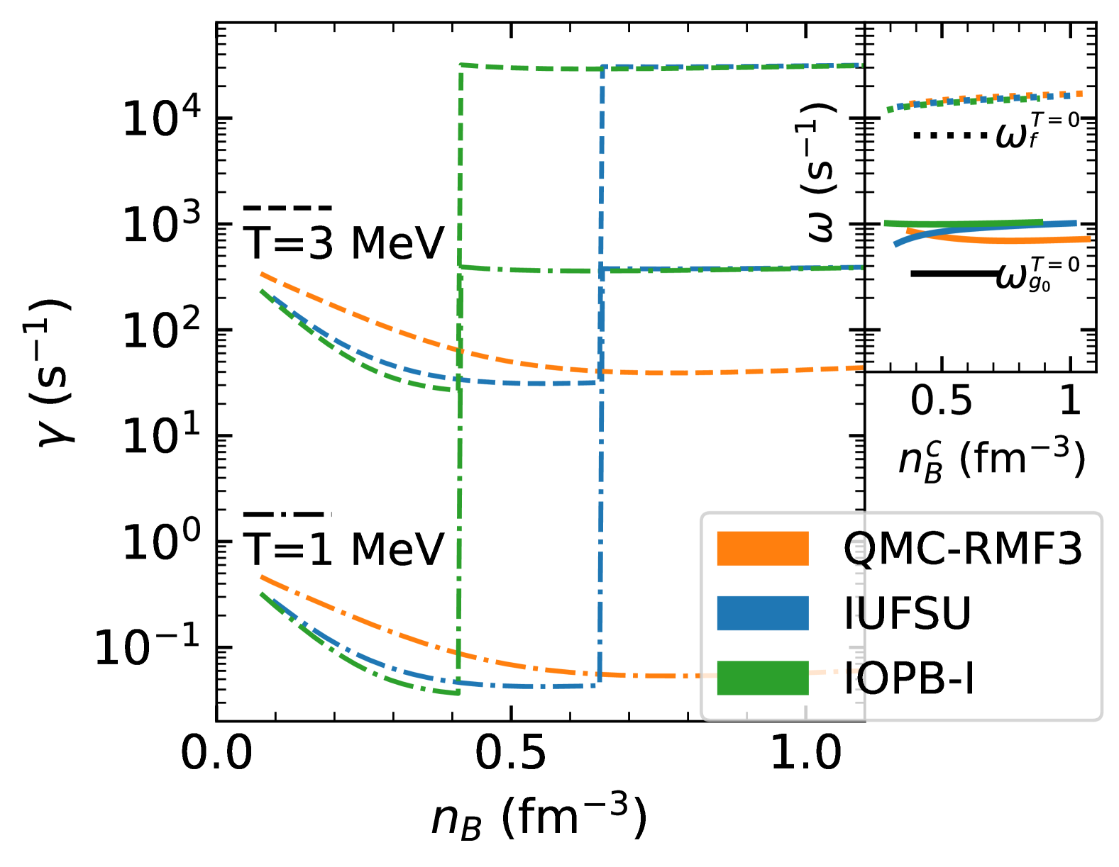
Figure 1: Left (main) panel shows the beta equilibration relaxation rate $\gamma$ defined in Eq. (7) for QMC-RMF3, IUFSU and IOPB-I EOSs at temperatures $T=1$ MeV (dot-dashed) and $T=3$ MeV (dashed). The solid (dashed) lines in the top right panel represent the $g$-mode ($f$-mode) frequency of cold NSs with various central baryon densities $n_{\rm B}^{c}$.

The calculation of the rates in Eq. (7) requires a microscopic model of nuclear matter that provides us not just with the EOS, but also with the dispersion relations of the nucleons. We calculate our results for three different EOSs, described below, in order to properly consider the range of possible $g$-mode physics.

In Fig. 1, we plot the beta equilibration rate $\gamma$ as a function of the baryon density. We include both the direct Urca processes ($n\rightarrow p+e^{-}+\bar{\nu}_{e}$ and $e^{-}+p\rightarrow n+\nu_{e}$) as well as the modified Urca processes ($n+N\rightarrow p+e^{-}+\bar{\nu}_{e}+N$ and $e^{-}+p+N\rightarrow n+\nu_{e}+N$, where $N$ is a neutron or proton). For simplicity, we calculate the rates of these processes in the Fermi surface approximation, which is valid for strongly degenerate nuclear matter (typically, $T\lesssim 1\text{ MeV}$) Alford and Harris (2018); Alford et al. (2021a). In this limit, only particles on the Fermi surface participate in the reactions. This constraint on the phase space gives rise to a direct Urca threshold density: below this density, direct Urca is kinematically forbidden because the neutron Fermi momentum is too big relative to the proton and electron Fermi momenta (equivalently, the proton fraction is too small). Modified Urca does not have such a density threshold and has a rate that is only weakly dependent on the baryon density Yakovlev et al. (2001). While, for convenience, we use the Fermi surface approximation in this work, as the temperature rises, contributions from particles away from the Fermi surface begin to dominate the reaction rates, causing a blurring (in density) of the direct Urca threshold Alford and Harris (2018); Alford et al. (2021a). The formulas for the Fermi surface approximation of the Urca rates are given in App. A and B of Ref. Most et al. (2024).

The rates shown in Fig. 1 were calculated in matter described by three different EOSs, each built from a relativistic mean-field theory (RMFT), QMC-RMF3 Alford et al. (2022, 2023), IUFSU Fattoyev et al. (2010), and IOPB-I Kumar et al. (2018). All of them agree with current astrophysical and theoretical constraints on the EOS Kumar et al. (2024a), but differ in their predictions of the composition of $npe$ matter, which leads to significantly different predictions of the Urca rates. Critically, they have different predictions for the direct Urca threshold. While QMC-RMF3 does not have a direct Urca threshold at all, IOPB-I has a threshold density of $n_{\rm{B},\mathrm{thr.}}=0.414~\mathrm{fm}^{-3}$, and IUFSU a threshold density of $n_{\rm{B},\mathrm{thr.}}=0.655~\mathrm{fm}^{-3}$.

At low density, in Fig. 1, direct Urca is forbidden for all EOSs and the rates are entirely due to modified Urca. As the density increases, the rates for two of the EOSs, IUFSU and IOPB-I, increase dramatically as the direct Urca threshold is passed. The QMC-RMF3 EOS always forbids direct Urca, as the proton fraction never rises above $1/9$ (c.f. Lattimer et al. (1991)). Equilibration rates at two different temperatures ($T=1\text{ and }3\text{ MeV}$) are shown: clearly, the equilibration rate is a strong function of temperature (see e.g., Fig. 8 in Harris (2024)). To the right of the main plot, we attached a plot of the oscillation frequencies of the $f$-mode and $g$-mode as a function of the central density of the neutron star (different from the x-axis of the left plot). This presentation allows us to compare the frequency of the density change of the matter $\omega$ with the rate at which beta equilibrium is restored $\gamma$. This ratio is the key quantity in determining the bulk-viscous damping of the oscillation modes and the disappearance of the $g$-mode at high temperature. Evidently, temperatures of a few MeV will make the beta equilibration rate comparable to the density oscillation frequency.

Applying the harmonic oscillation ansatz ${\rm e}^{i\omega t}$ for all perturbations in Eq. (7), we obtain

$$\Delta{\delta\mu} = \dfrac{\left.\dfrac{\partial{\delta\mu}}{\partial n_{\rm B}}\right|_{x_{\delta},S}\Delta n_{\rm B}}{1+\dfrac{\gamma}{i\omega}}\,.$$ (8)

We substitute Eq. (8) into Eq. (2), yielding

$$\Delta p = \dfrac{p\Gamma}{n_{\rm B}}\Delta n_{\rm B}\,,$$ (9)

where the complex-valued effective adiabatic index for a damped oscillation of frequency $\omega$ is given by

$$\Gamma = \dfrac{n_{\rm B}}{p}\left[\left.\dfrac{\partial p}{\partial n_{\rm B}}\right|_{{\delta\mu},S}+\dfrac{\left.\dfrac{\partial p}{\partial{\delta\mu}}\right|_{n_{\rm B},S}\left.\dfrac{\partial{\delta\mu}}{\partial n_{\rm B}}\right|_{x_{\delta},S}}{1+\dfrac{\gamma}{i\omega}}\right].$$ (10)

This expression can be recast in a more transparent form:

$$\Gamma = \Gamma_{\rm eq}+\dfrac{\Gamma_{\rm ad}-\Gamma_{\rm eq}}{1+\dfrac{\gamma}{i\omega}}\,,$$ (11)

$$\Gamma_{\rm ad} = \dfrac{n_{\rm B}}{p}\left.\dfrac{\partial p}{\partial n_{\rm B}}\right|_{x_{\delta},S}\,,$$ (12)

$$\Gamma_{\rm eq} = \dfrac{n_{\rm B}}{p}\left.\dfrac{\partial p}{\partial n_{\rm B}}\right|_{{\delta\mu},S}\,,$$ (13)

where $\Gamma_{\rm ad}$ and $\Gamma_{\rm eq}$ characterize the compressibility of matter in the slow and fast limits of beta equilibration, respectively. The computation of these derivatives from the EOS tables, using $n_{\rm B}$, $x$ and $T$ as input variables, is described in detail in Appendix A.

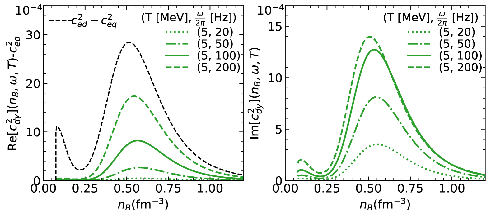
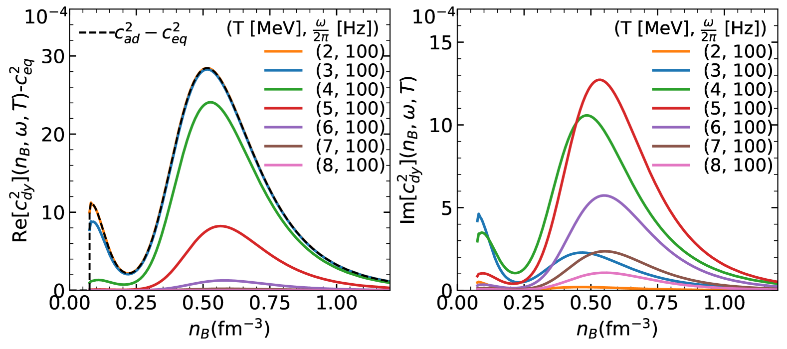
Figure 2: Real (left panels) and imaginary (right panels) part of the dynamic sound speed squared for the QMC-RMF3 EOS. For the real part, the equilibrium sound speed squared is used as a reference. The black dashed line represents the difference between adiabatic and equilibrium squared sound speeds. The upper two panels correspond to fixed temperature $T=5$ MeV while varying frequency $\omega/2\pi=[20,50,100,200]$ Hz; the bottom two panels represent fixed frequency $\omega/2\pi=100$ Hz while varying temperature from 2 to 8 MeV. Note the different scales of y-axes in real and imaginary parts.

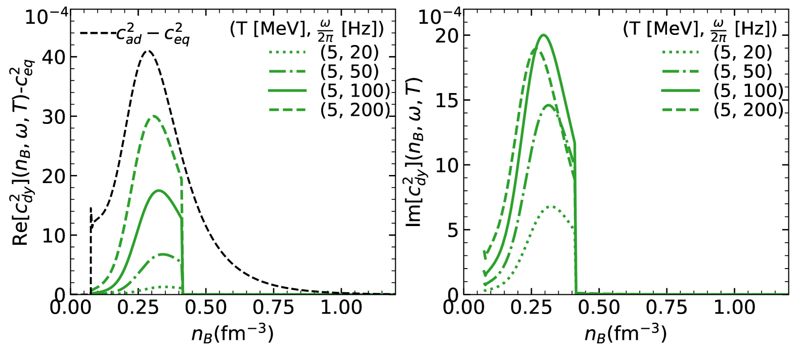
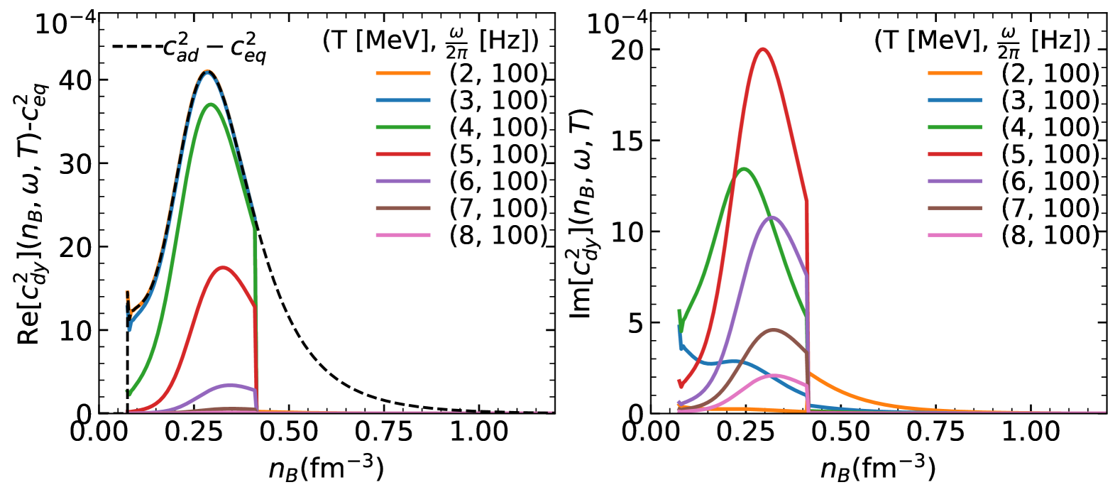
Figure 3: Same as Fig. 2, but for the IOPB-I EOS.

The dynamic sound speed squared $c_{\rm dy}^{2}$ which incorporates finite-temperature viscous effects, is defined as

$$c_{\rm dy}^{2} = \dfrac{p}{\varepsilon+p}\,\Gamma=c_{\rm eq}^{2}+\dfrac{c_{\rm ad}^{2}-c_{\rm eq}^{2}}{1+\dfrac{\gamma}{i\omega}}\,,$$ (14)

where the equilibrium and adiabatic sound speed squared $c_{\rm eq}^{2}$ and $c_{\rm dy}^{2}$ are given by

$$c_{\rm eq}^{2}=\dfrac{p}{\varepsilon+p}\,\Gamma_{\rm eq}\,,\qquad c_{\rm ad}^{2}=\dfrac{p}{\varepsilon+p}\,\Gamma_{\rm ad}\,.$$ (15)

The real and imaginary parts of the dynamic sound speed squared are then given by

$${\rm Re}\left[c_{\rm dy}^{2}\right] = c_{\rm eq}^{2}+\left(c_{\rm ad}^{2}-c_{\rm eq}^{2}\right)\dfrac{\omega^{2}}{\omega^{2}+\gamma^{2}}\,,$$ (16)

$${\rm Im}\left[c_{\rm dy}^{2}\right] = \left(c_{\rm ad}^{2}-c_{\rm eq}^{2}\right)\dfrac{\omega\gamma}{\omega^{2}+\gamma^{2}}.$$ (17)

The imaginary part, ${\rm Im}\left[c_{\rm dy}^{2}\right]$, is directly related to the bulk viscosity coefficient $\zeta$, which is defined via the energy dissipation rate $\mathop{{\rm d}\varepsilon}/\mathop{{\rm d}t}=-\zeta(\nabla\cdot\mathbf{v})^{2}$, since the bulk viscosity coefficient is also equal to the EOS-related factor times the resonance expression $\gamma/\left(\gamma^{2}+\omega^{2}\right)$ Harris (2024). Using thermodynamic identities and the definitions of the adiabatic indices [Eqs. (12) and (13)], the bulk viscosity can be expressed as

$$\zeta = \dfrac{\varepsilon+p}{\omega}{\rm Im}\left[c_{\rm dy}^{2}\right]$$ (18)

$$= 4.3\times 10^{29}\rm{~g~cm}^{-1}\rm{~s}^{-1}\left(\dfrac{\omega/{2\pi}}{100\rm{~Hz}}\right)^{-1}\,$$

$$\times\left(\dfrac{(\varepsilon+P)/c^{2}}{3\times 10^{14}\rm{~g~cm}^{-3}}\right)\left(\dfrac{{\rm Im}\left[c_{\rm dy}^{2}\right]}{0.001}\right).$$

For neutron star matter, the adiabatic sound speed is usually very close to the equilibrium sound speed ($c_{\rm ad}^{2}-c_{\rm eq}^{2}\lesssim 0.01$), and therefore the second term on the right-hand side of Eq. (14) is small. As a result, the imaginary part of the dynamic sound speed squared is small, while the real part lies between the adiabatic and equilibrium squared sound speeds. The source of the difference between $c_{\rm ad}^{2}$ and $c_{\rm eq}^{2}$ in our paper is the gradient in the proton fraction $x$, not a gradient in the entropy per particle $S$. To demonstrate the dynamic sound speed squared $c_{\rm dy}^{2}$, we plot the real and imaginary part of $c_{\rm dy}^{2}$ versus $n_{\rm B}$ for various temperatures $T$ and frequencies $\omega$ for the QMC-RMF3 EOS in Fig. 2 and for the IOPB-I EOS in Fig. 3. QMC-RMF3 shows double peaks in $c_{\rm ad}^{2}-c_{\rm eq}^{2}$ due to a plateau in the equilibrium composition $x_{\rm eq}$ around $n_{\rm B}=0.2$ fm^-3. The IOPB-I curve only has one peak and terminates at $n_{\rm B}=0.414$ fm^-3, beyond which $c_{\rm dy}^{2}\approx c_{\rm eq}^{2}$ due to the onset of the direct Urca process.

The real part of the dynamic sound speed is the adiabatic sound speed at low temperatures (or in the high-frequency limit), and as temperature is increased (or frequency is lowered), it decreases to the equilibrium sound speed. The imaginary part of the dynamic sound speed is non-monotonic with respect to temperature – it starts from zero at low temperatures and then increases until reaching a peak at the resonant temperature where $\gamma=\omega$. As the temperature (and thus $\gamma$) further increases, the imaginary part of the dynamic sound speed drops to zero. This resonant behavior is, naturally, just like the resonant behavior of bulk viscosity Harris (2024).

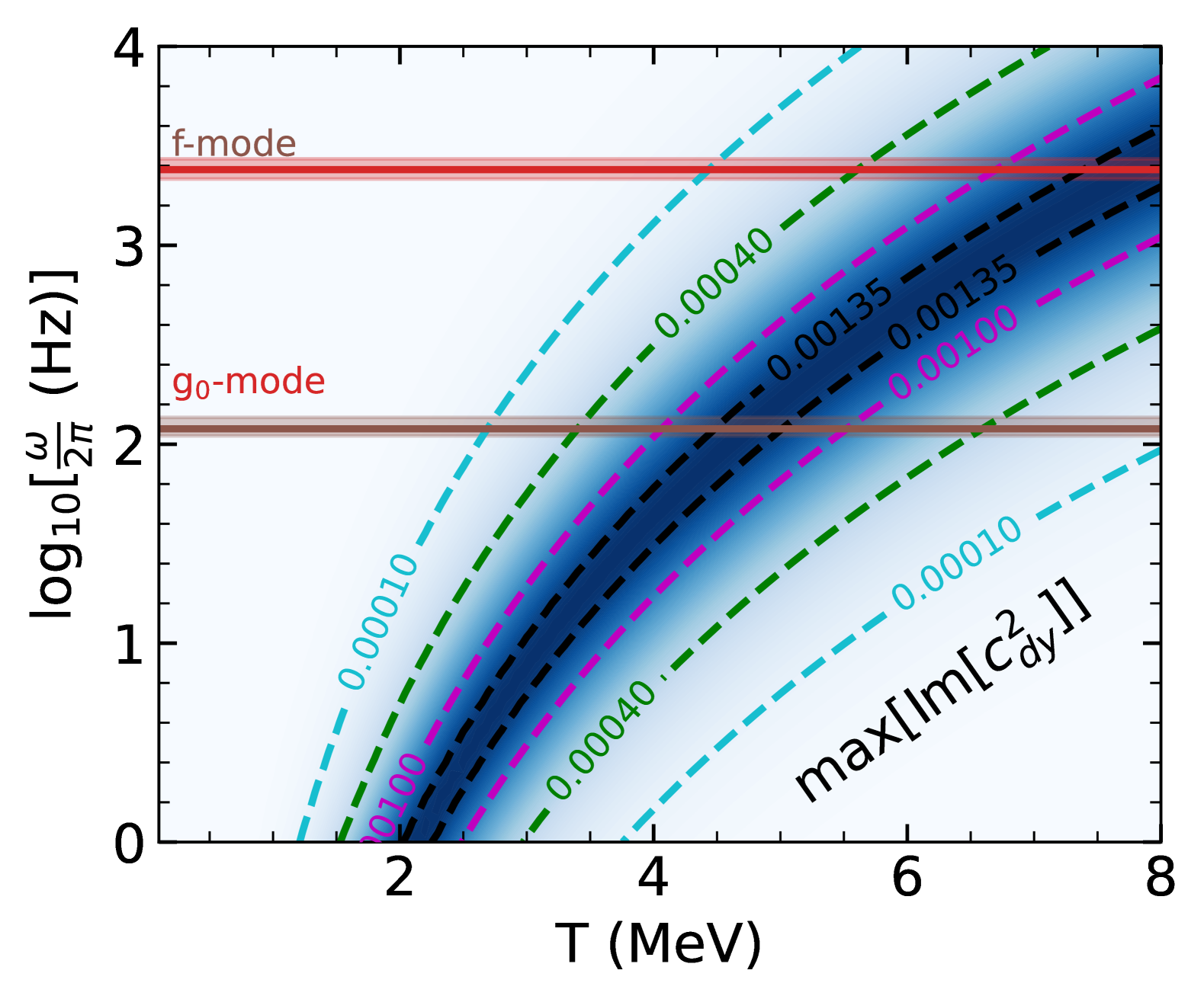
Figure 4: The dashed contour shows the maximum (across all densities) of the imaginary part of the dynamic sound speed squared for QMC-RMF3 (top) and IOPB-I (bottom). The dark blue region corresponds to the resonant peak, where bulk viscosity is most effective at damping oscillations. The horizontal brown and red bands represent typical $f$-mode and $g$-mode frequencies (at zero temperature) for NSs of various masses, with the central line corresponding to a 1.4 ${\rm M}_{\odot}$ NS.

In Fig. 4, we show the maximum value (across all densities) of the imaginary part of the dynamic sound speed squared in the temperature-frequency plane. This plot depicts the resonant behavior described above. There is only one resonant peak for QMC-RMF3, while for IOPB-I, there exist two distinct resonant bands corresponding to the direct and modified Urca processes, respectively. These peaks are unrelated to the double-peak structure discussed in the context of Fig. 2. The direct Urca process, with a higher reaction rate, has a resonant peak at a higher frequency or a lower temperature compared to the modified Urca process peak. Typical $f$-mode and $g$-mode frequencies at zero temperature are shown in Fig. 4.

In this work, the crust EOSs in beta equilibrium are constructed with the compressible liquid droplet model with fixed surface tension parameters $\sigma_{s}=1.2$ MeV fm^-2, $S_{S}=48$ MeV Lattimer and Swesty (1991). Below the crust-core transition density, the adiabatic sound speed is set equal to the equilibrium sound speed, as our focus is on core $g$-modes following Ref. Jaikumar et al. (2021). This is justified because the adiabatic sound speed in the crust has only a limited impact on the properties of core $g$-modes Sun et al. (2025).

III Mode equations

The components of the interior metric tensor for a spherically symmetric, non-rotating star are defined by

$${\rm d}s^{2}=-{\rm e}^{\nu(r)}{\rm d}t^{2}+{\rm e}^{\lambda(r)}{\rm d}r^{2}+r^{2}({\rm d}\theta^{2}+\sin^{2}\theta{\rm d}\phi^{2}).$$ (20)

Following e.g., Ref. Jaikumar et al. (2021), we solve the general relativistic non-radial mode equations in the relativistic Cowling approximation, which ignores perturbations of the metric tensor. The mode equations are

$$\dfrac{{\rm d}U}{{\rm d}r}={} \dfrac{g}{c_{\rm dy}^{2}}U+{\rm e}^{\lambda/2}\left(\dfrac{\ell(\ell+1)}{\omega^{2}}{\rm e}^{\nu}-\dfrac{r^{2}}{c_{\rm dy}^{2}}\right)V,$$ (21)

$$\dfrac{{\rm d}V}{{\rm d}r}={} {\rm e}^{\lambda/2-\nu}\dfrac{\omega^{2}-N^{2}}{r^{2}}U+g\left(\dfrac{1}{c_{\rm eq}^{2}}-\dfrac{1}{c_{\rm dy}^{2}}\right)V,$$ (22)

where $U$ and $V$ are related to the radial component of the Lagrangian displacement field $\xi_{r}$ and the Eulerian perturbation of the pressure $\delta p$ by

$$U=r^{2}{\rm e}^{\lambda/2}\xi_{r},\qquad V=\dfrac{\delta p}{\varepsilon+p}.$$ (23)

$\ell$ is the degree of the vector spherical harmonic representing the angular dependence of the displacement field, which we restrict to $\ell=2$. The gravitational acceleration $g$ is

$$g=-\dfrac{1}{\varepsilon+p}\dfrac{{\rm d}p}{{\rm d}r}=\dfrac{1}{2}\dfrac{{\rm d}\nu}{{\rm d}r}.$$ (24)

The two sound speeds squared $c_{\rm eq}^{2}$ and $c_{\rm dy}^{2}$ are given by Eq. (14) and Eq. (15). Note that $c_{\rm dy}^{2}$ replaces $c_{\rm ad}^{2}$ from the original formulation of the mode equations, which are recovered in the limit that $\gamma\rightarrow 0$. Finally, the Brunt–Väisälä frequency squared $N^{2}$ is

$$N^{2}=g^{2}\left(\dfrac{1}{c_{\rm eq}^{2}}-\dfrac{1}{c_{\rm dy}^{2}}\right){\rm e}^{\nu-\lambda}.$$ (25)

Note that $N^{2}$ is now complex due to the inclusion of $c_{\rm dy}^{2}$.

The boundary conditions at $r=0$ are

$$U(r=0)= \dfrac{\ell}{\omega^{2}}Y_{0}r^{\ell+1},$$ (26)

$$V(r=0)= \dfrac{\varepsilon}{\varepsilon+p}Y_{0}r^{\ell},$$ (27)

where $Y_{0}$ is a constant that shifts the overall amplitude of the oscillation mode, which is itself unconstrained. The $r=R$ boundary condition is the vanishing of the Lagrangian pressure perturbation at $\Delta p(r=R)=0$, which is equivalent to

$$0=V(r=R)-\dfrac{1}{2R^{2}}U(r=R){\rm e}^{-\lambda(r=R)/2}\left.\dfrac{{\rm d}\nu}{{\rm d}r}\right|_{r=R}.$$ (28)

Since $c_{\rm dy}^{2}$ is complex, the solutions to the mode equations are also complex, therefore Eqs. (21) and (22) can be solved by splitting them into real and imaginary parts. This is presented in Appendix B. We performed independent calculations of the oscillation modes using complex equations and then splitting into real and imaginary parts, obtaining identical results in each case.

To assess the validity of the relativistic Cowling approximation, we also carried out linearized full general relativity (GR) calculations of non-radial $f$-mode and $g$-modes, following the formalism outlined in the appendix of Ref. Zhao and Lattimer (2022). The system of differential equations governing linear non-radial oscillations in full GR reduces to Eqs. (21) and (22) of the relativistic Cowling approximation when the metric perturbations are neglected, as shown explicitly in Ref. Zhao et al. (2022).

IV Results

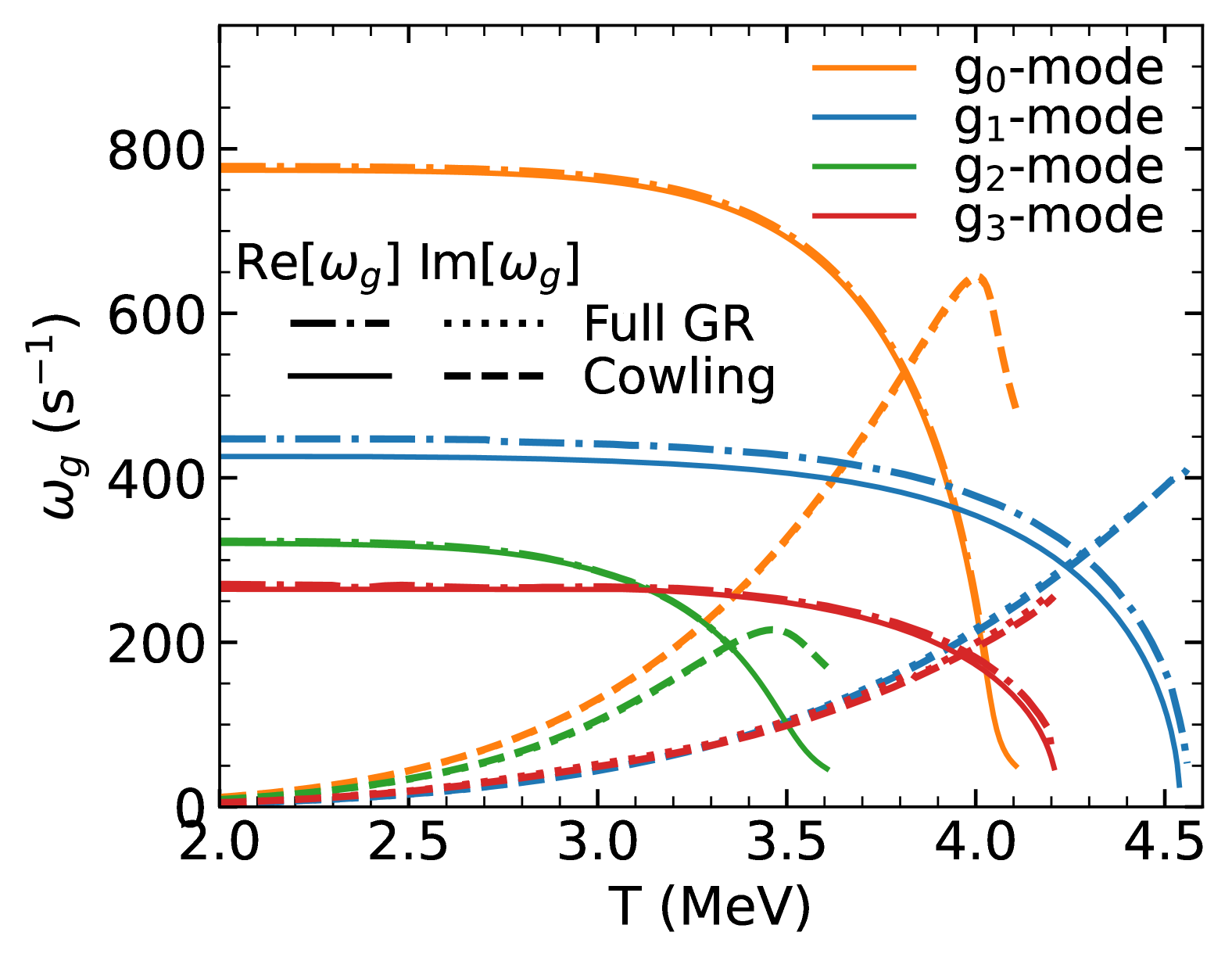
Figure 5: Real and imaginary parts of the frequencies of the fundamental and the first three harmonic $g$-modes for a $1.4~{\rm M}_{\odot}$ neutron star versus varying temperature for the QMC-RMF3 EOS. The imaginary part of the full GR calculation (dotted) largely overlaps with that of the calculation with Cowling approximation (dashed), and the real parts of the full GR calculation (dash-dotted) and Cowling approximation (solid) are also very similar. We define the ordering of $g$-modes by their smooth asymptotic eigenmode at zero temperature.

(a)

(b)

Figure 6: Same as Fig. 5 but for the IUFSU EOS (panel (a)) and the IOPB-I EOS (panel (b)).

To examine the effect of weak interactions on the damping of $g$-modes, we computed the complex $g$-mode frequencies of $1.4~{\rm M}_{\odot}$ NSs at various temperatures for the three selected EOSs. Fig. 5 shows the real and imaginary parts of the $g$-mode frequency as a function of temperature for the QMC-RMF3 EOS, with the results compared between using and not using the Cowling approximation.

The Cowling approximation introduces only a very small error compared to the full GR calculation for the $g$-modes. Therefore, for the remainder of the paper we only consider results obtained using the Cowling approximation. As the temperature increases and thus the bulk viscosity increases, the real part of $g$-mode frequency decreases while the imaginary part increases. The real parts of the even harmonic $g$-modes vanish at lower temperatures compared to the odd $g$-modes because of the double peaks in the sound speed squared difference shown in Fig. 2. This leads to an interchange in the temperature at which these modes vanish, such that the $g_{1}$ and $g_{3}$-modes vanish at higher temperatures than the $g_{0}$ and $g_{2}$-modes. In comparison, Fig. 6 shows the $g$-mode frequencies for the IUFSU and IOPB-I EOSs. Since these two EOSs have only one peak in their squared sound speed differences, they do not display a characteristic difference between the even and odd $g$-modes like that shown for the QMC-RMF3 EOS.

Figure 7: Frequency (solid and dot-dashed) and damping time (dashed and dotted) of the $f$-mode calculated with and without Cowling approximation. The damping time of $g$-modes in Fig. 5 is plotted as the blue region for comparison. The bottom of the blue region corresponds to the lowest order $g$-mode.

We also calculated the $f$-mode of a 1.4 ${\rm M}_{\odot}$ NS at various temperatures as shown in Fig. 7, and found that the $f$-mode frequency is extremely insensitive to temperature. The real part of the frequency calculated with the Cowling approximation is 26% larger than that with the full GR calculation. The imaginary part is much smaller, so the damping time $\tau=1/{\rm Im}[\omega_{f}]$ is plotted instead. Since the Cowling approximation calculation ignores the damping due to gravitational waves completely, it results in a damping time $\approx 10$ seconds, much larger than the gravitational-wave damping time of the $f$-mode, $\approx 0.1$ seconds. Therefore, the damping introduced by bulk viscosity is much weaker than the damping from gravitational waves even at the resonant peak shown in Fig. 4. This is not surprising given that $f$-mode is known to be very close to the Kelvin mode, a divergence-free oscillation mode. The analytical solution for the Kelvin mode is very close to $f$-mode calculated with full GR. Therefore, the fluid goes through compression and expansion only in the Eulerian frame but remains largely uncompressed in the Lagrangian frame. This provides a direct validation that the bulk viscosity is not important for the linear $f$-mode oscillation regardless of temperature.

(a) QMC-RMF3, $g_{0}$-mode

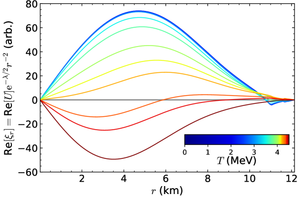
(b) QMC-RMF3, $g_{1}$-mode

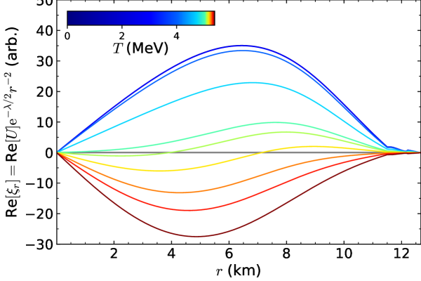
(c) IUFSU, $g_{0}$-mode

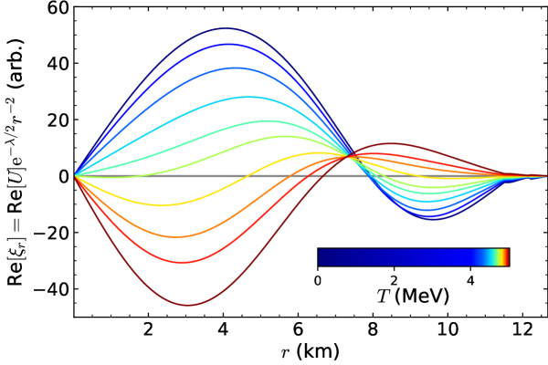
(d) IUFSU, $g_{1}$-mode

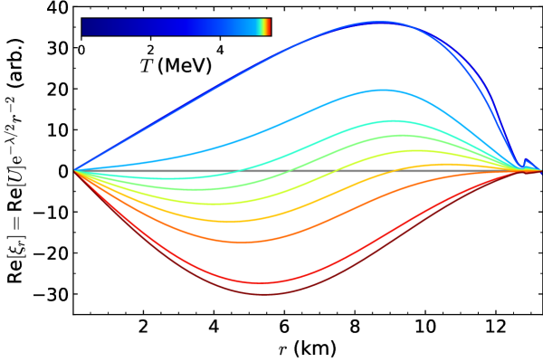
(e) IOPB-I, $g_{0}$-mode

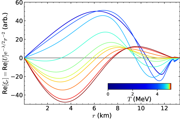
(f) IOPB-I, $g_{1}$-mode

Figure 8: Real part of the radial displacement field $\xi_{r}(r)$ for the fundamental $g_{0}$-mode (left panels) and first harmonic $g_{1}$-mode (right panels) as a function of the temperature, for three different EOSs: QMC-RMF3 (top row), IUFSU (middle row), and IOPB-I (bottom row). Note the changes in node number as the temperature increases, particularly within the final $\sim 0.5$ MeV of the color bar.

When the bulk viscosity is included in the mode calculation, the resulting mode frequencies are no longer purely real numbers, so Sturm–Liouville theory does not strictly apply. This means that the displacement fields for the modes no longer follow the expected pattern whereby the number of internal modes of the $n$th harmonic mode is $n$, with the fundamental mode having zero internal nodes, the first harmonic mode having one internal node, etc. Instead, as the temperature increases and the bulk viscosity plays an increasingly important role, with the imaginary part of the mode frequency increasing, we observe that the number of internal nodes of the mode displacement field can change compared to the expectation from Sturm–Liouville theory.

We demonstrate this in Fig. 8 that shows the evolution in the displacement field for the fundamental and first harmonic $g$-modes as a function of the temperature for the QMC-RMF3 EOS. First, examining the fundamental mode in panel (a), one finds that for low temperatures $T\lesssim 3.5$ MeV, the displacement field takes an expected form for a fundamental mode with zero internal nodes, but the displacement field below $r\sim 6$ km moves closer to the Re$[\xi_{r}]=0$ axis. As $T=4$ MeV is approached, the displacement field then crosses this axis close to $r=0$, with this node moving to higher $r$ as the temperature increases, thus giving first a single internal node and then three internal nodes. At the highest temperatures examined, when the real part of the mode frequency becomes much smaller than the imaginary part, the displacement field has two internal nodes. The behavior of the first harmonic mode displacement field in panel (b) also violates the typical behavior expected from Sturm–Liouville theory: as the temperature approaches towards $T=4$ MeV, the mode first becomes nodeless, with its node near $r\approx 11$ km vanishing, then a new node develops at $r=0$, moving to larger $r$ as $T$ increases before vanishing again at the highest temperature examined. The IUFSU and IOPB-I EOSs show similar behavior, respectively, with nodes appearing or disappearing as the temperature increases toward the limit where the imaginary part of $\omega_{g}$ exceeds the real part.

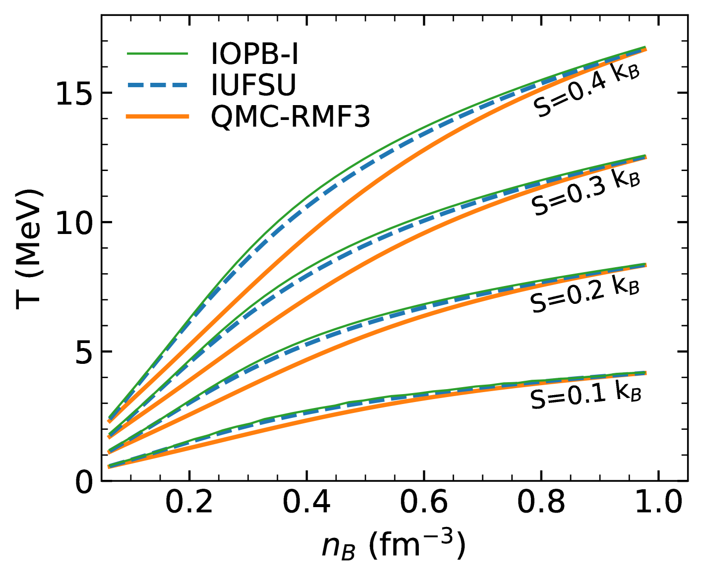
Figure 9: Temperature profiles at fixed entropy per baryon for three (QMC-RMF3, IUFSU, IOPB-I) EOSs. These profiles are obtained by solving the equations of motion numerically in weak chemical equilibrium and at finite temperatures. At each density point, the entropy is calculated for several temperature points and then linearly interpolated in order to apply a root-finding algorithm to determine the desired constant entropy profile.

To investigate the impact of bulk viscosity on neutron stars with varying thermal structures Kumar et al. (2024b); Ghosh et al. (2024), we first compute temperature profiles at fixed entropy per baryon values, $S=s/n_{\rm B}=\{0.1,0.2,0.3,0.4\}\,k_{B}$, for three different EOSs as shown in Fig. 9. In the degenerate limit of a neutron gas, the entropy per baryon follows the relation $S=\pi^{2}\,k_{B}^{2}Tm_{\mathrm{L}}/{k_{\mathrm{F}}^{2}}$, where $k_{\mathrm{F}}=(3\pi^{2}n_{\rm B})^{1/3}$ is the Fermi momentum, and the Landau effective mass is defined as $m_{\mathrm{L}}=k_{\mathrm{F}}\left(dk_{\mathrm{F}}/d\epsilon_{\mathrm{F}}\right)$, which reduces to $m_{\mathrm{L}}=\sqrt{k_{\mathrm{F}}^{2}+m_{D}^{2}}$, where $m_{D}$ is the Dirac effective mass $m^{*}$ in the RMF model. Consequently, at fixed entropy per baryon, the temperature scales as $T\propto n_{\rm B}^{2/3}/m_{\mathrm{L}}$, where the Landau effective mass $m_{\mathrm{L}}$ exhibits different density dependencies across the three EOSs. At subnuclear densities, where $k_{\mathrm{F}}\ll m_{D}$, the Landau mass approaches $m_{\mathrm{L}}\approx m_{D}$, yielding the scaling $T\propto n_{\rm B}^{2/3}/m_{D}$. At several times nuclear saturation density, where $k_{\mathrm{F}}\gg m_{D}$, one finds $m_{\mathrm{L}}\approx k_{\mathrm{F}}\propto n_{\rm B}^{1/3}$, and the temperature scales as $T\propto n_{\rm B}^{1/3}$. This trend of the power-law index decreasing from 2/3 to 1/3 appears in Fig. 9.

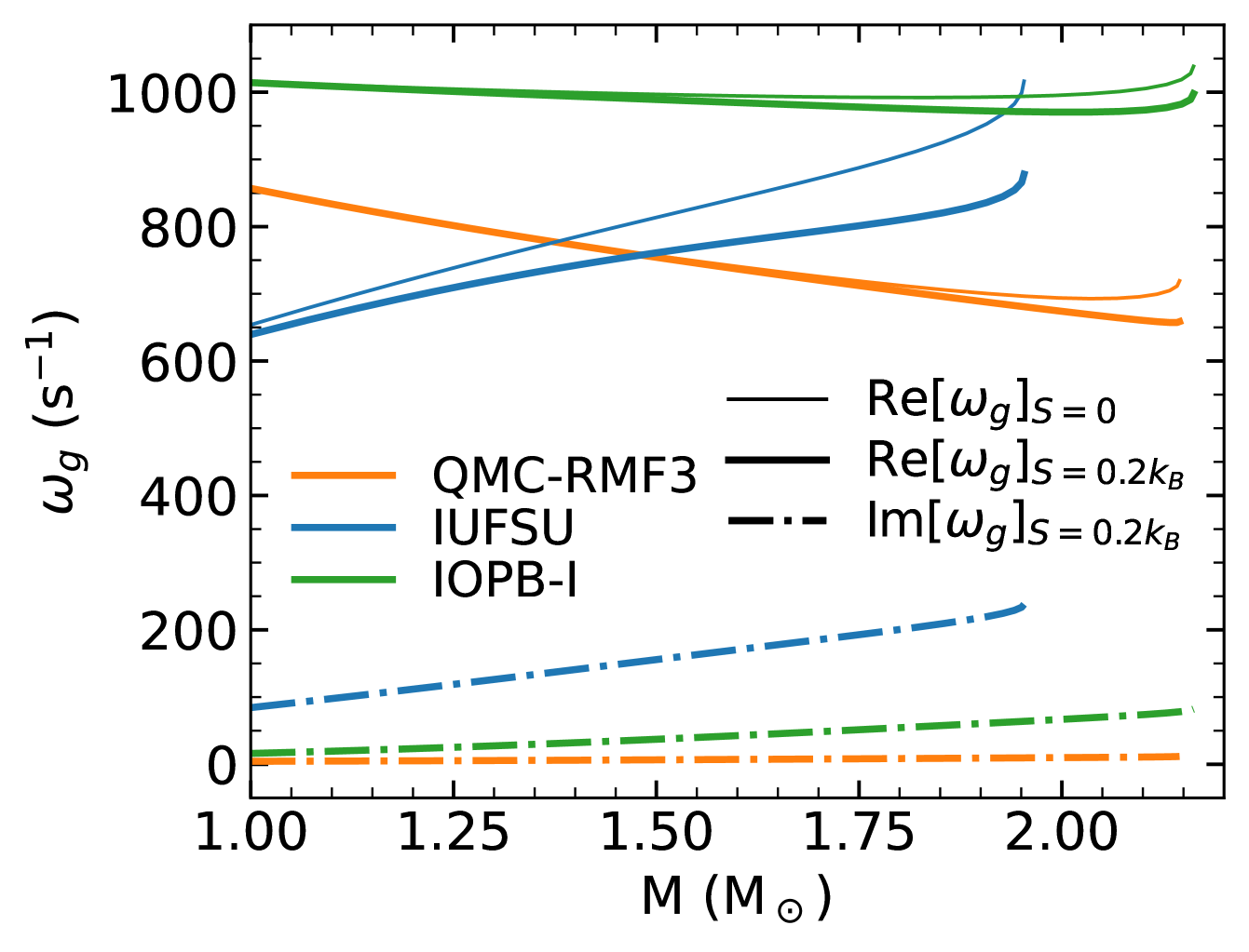
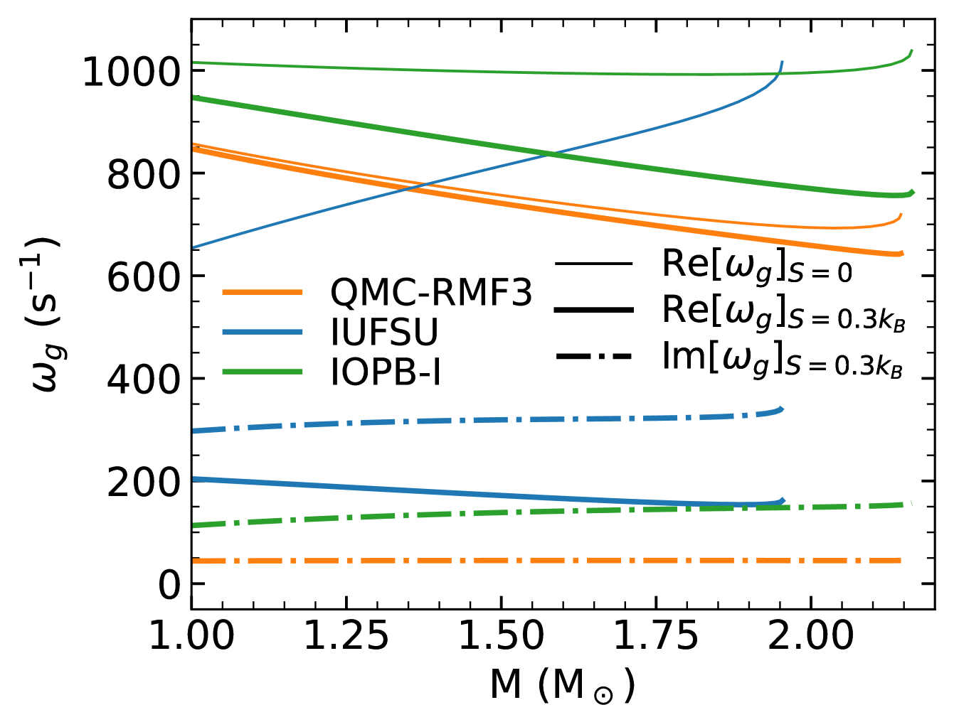
Figure 10: $g$-mode frequency as a function of NS mass at fixed entropy per baryon $S=0.2\,k_{B}$ (top), $S=0.3\,k_{B}$ (middle), and $S=0.4\,k_{B}$ (bottom). The real (thick solid lines) and imaginary (dot-dashed lines) parts of the frequency are shown, and the thin solid line refer to the cold adiabatic $g$-mode frequency in the absence of viscosity, which has no imaginary part. Results for three different EOSs are shown, and the calculations were performed within the Cowling approximation.

Figure 11: Real (solid) and imaginary (dashed) parts of the difference between the dynamic and equilibrium sound speed squared, ${\rm Re}[c_{\rm dy}^{2}-c_{\rm eq}^{2}]$ and ${\rm Im}[c_{\rm dy}^{2}]$, as functions of the baryon number density $n_{\rm B}$ at fixed values of the entropy per baryon, $S=0.3\,k_{B}$ (thin) and $S=0.4\,k_{B}$ (thick). Results are shown for the QMC-RMF3 EOS at an oscillation frequency $f=100$ Hz (blue) and for the IUFSU EOS at $f=30$ Hz (orange). The density regions where ${\rm Re}[c_{\rm dy}^{2}-c_{\rm eq}^{2}]>{\rm Im}[c_{\rm dy}^{2}]$ can support local $g$-mode oscillations, whereas regions dominated by the imaginary part indicate strong damping and therefore the mode propagation is suppressed.

Using these temperature profiles, we compute the $g_{0}$-mode frequencies as a function of the stellar mass, shown in Fig. 10. For comparison, the zero entropy ($T=0$) $g_{0}$-modes, which are purely real, are also shown as thin lines. The most notable feature is that the real part of the frequency for the $g_{0}$-mode with the IUFSU EOS decreases much more with increasing $S$ than for the other two EOSs, such that it vanishes at $S=0.4\,k_{B}$. This can be explained by examining the temperature dependence of the sound speed squared difference $c_{\rm dy}^{2}-c_{\rm eq}^{2}$ for the IUFSU EOS and then comparing it to those obtained for the other two EOSs. At the crust-core transition density $n_{\rm B}\approx 0.08$ fm^-3, the constant entropy $S=0.4\,k_{B}$ profile corresponds to a temperature $T\approx 3$ MeV according to Fig. 9. From Figs. 2–3, for the QMC-RMF3 and IOPB-I EOSs, the real part of $c_{\rm dy}^{2}-c_{\rm eq}^{2}$ is larger than the imaginary part at this temperature and density. Though the density increases and temperature for fixed $S$ correspondingly increases deeper inside the star, the real part of $c_{\rm dy}^{2}-c_{\rm eq}^{2}$ being larger than the imaginary part near the crust-core transition is sufficient for the $g_{0}$-mode to be supported. However, for the IUFSU EOS, the real and imaginary parts of $c_{\rm dy}^{2}-c_{\rm eq}^{2}$ at $T\approx 3$ MeV are already nearly the same, and since the imaginary part only becomes greater and the real part smaller as the density increases and the temperature simultaneously increases for fixed $S$, the $g_{0}$-mode vanishes for this and larger values of $S$. This is shown explicitly in Fig. 11, which compares the real and imaginary parts of the sound speed squared difference for $S=0.3\,k_{B}$ and $0.4\,k_{B}$ for the QMC-RMF3 and IUFSU EOSs as functions of the density, computed at values of $\omega$ approximating the $g_{0}$-mode frequency. For both values of $S$ for the QMC-RMF3 EOS, there is a region of the star where ${\rm Re}[c_{\rm dy}^{2}-c^{2}_{\rm eq}]>{\rm Im}[c_{\rm dy}^{2}]$, which is also the case for the IUFSU EOS when $S=0.3\,k_{B}$. However, ${\rm Im}[c_{\rm dy}^{2}]>{\rm Re}[c_{\rm dy}^{2}-c^{2}_{\rm eq}]$ for the IUFSU EOS at $S=0.4\,k_{B}$, indicating that there is no $g_{0}$-mode for this EOS at this value of $S$.

V Conclusions and outlook

Thermal effects on the $g$-modes of neutron stars are of increasing interest because these modes will be excited in protoneutron stars and post-merger remnant neutron stars. In this work, we introduce the concept of the dynamic sound speed squared, $c_{\rm dy}^{2}$, which captures the impact of bulk viscous effects in hot neutron star matter at temperatures of a few MeV. Unlike conventional adiabatic and equilibrium sound speeds, the dynamic sound speed incorporates the frequency-dependent damping effects of weak interaction equilibration, leading to a complex-valued expression. The real part of $c_{\rm dy}^{2}$ lies between the equilibrium sound speed squared $c_{\rm eq}^{2}$ and the adiabatic sound speed squared $c_{\rm ad}^{2}$, while its imaginary part encodes dissipative effects associated with the bulk viscosity, $\zeta={\rm Im}\left[c_{\rm dy}^{2}\right]{(\varepsilon+P)}/{\omega}$. We demonstrate that the imaginary part ${\rm Im}[c_{\rm dy}^{2}]$ exhibits a resonant peak when the beta equilibration rate $\gamma$ becomes comparable to the oscillation frequency $\omega$. To further characterize this behavior, we identify the resonant region by mapping the peak values of ${\rm Im}[c_{\rm dy}^{2}]$ (across varying densities) in the T-$\omega$ plane and then compare it to the characteristic frequencies of neutron star oscillation modes. For EOSs where direct Urca is kinematically forbidden on the Fermi surface (e.g., QMC-RMF3), we find a single resonance band that starts at zero frequency around $T\approx 2$ MeV and extends to $\omega=100$ Hz at $T\approx 4.5$ MeV, continuing beyond. In contrast, EOSs with a direct Urca threshold exhibit significantly faster beta equilibration rates $\gamma$ at densities above the threshold, leading to an additional resonance band at lower temperatures or higher frequencies, as seen in the right panel of Fig. 4 for IOPB-I.

The relativistic Cowling approximation which ignores metric perturbations is widely used in the calculations of $g$-modes due to its simplicity and accuracy. Our results confirm that even with the inclusion of bulk viscosity, the Cowling approximation remains a reliable method for computing $g$-modes, introducing only a small error compared to the full GR calculations. Nevertheless, for the $f$-mode, we confirm that the Cowling approximation overestimates the frequency by approximately 26%, making it less accurate for studying $f$-mode oscillations Sotani and Takiwaki (2020); Zhao and Lattimer (2022); Rather et al. (2024).

We investigate the effects of weak interactions and bulk viscosity on the $g$-modes and $f$-mode of neutron stars by computing their complex frequencies at different temperatures. As the temperature increases, bulk viscosity becomes more significant, leading to a decrease in the real part of the $g$-mode frequency as well as an increase in its imaginary part, indicating stronger damping. We observe that for EOSs with a double-peak structure in the sound speed squared difference (e.g., QMC-RMF3), the even and odd $g$-modes behave differently, whereas EOSs with a single peak (e.g., IUFSU, IOPB-I) do not exhibit this distinction. Additionally, we find that at sufficiently high temperatures, bulk viscosity alters the nodal structure of the displacement field, deviating from the expectations of Sturm–Liouville theory, as modes develop additional nodes.

We find that the $f$-mode frequency remains largely insensitive to temperature and that the bulk viscosity has a negligible effect on its damping compared to gravitational wave emission. This is consistent with the fact that the $f$-mode is very close to the Kelvin mode, which is nearly divergence-free. In the Lagrangian frame, fluid elements undergo minimal compression, significantly reducing the impact of bulk viscosity on the mode’s dissipation.

The stark contrast between the effects of bulk viscosity on the $f$- and $g$-modes is crucial for understanding its role in shaping the peak gravitational-wave frequency observed in post-merger remnants. Since the $f$-mode emits gravitational waves far more efficiently than $g$-modes, the gravitational-wave peak frequency is often dominated by $f$-mode oscillations Ng et al. (2021), and in such cases, the bulk viscosity is expected to have only a minor impact on the gravitational-wave signal, as suggested in Refs. Radice et al. (2022); Zappa et al. (2023). However, if the peak frequency contains significant contributions from other modes, e.g. $g$-modes, then the bulk viscosity may substantially alter both the post-merger dynamics and the emitted gravitational waves Most et al. (2024); Hammond et al. (2023). In our linearized general relativistic analysis, the $f$- and $g$-modes are treated as a linearly independent basis in the Hilbert space of fluid perturbations. Nonetheless, non-linear coupling between these modes may become significant in the highly dynamic environment of post-merger simulations. In such scenarios, the bulk viscous damping of $g$-modes might indirectly influence the gravitational-wave signal via energy transfer or mode mixing with the dominant $f$-mode.

Our analysis shows that at temperatures of a few MeV, beta equilibration becomes rapid enough to significantly affect the frequency and damping time of $g$-modes. In addition to examining $g$-modes at constant temperature, we also computed $g$-modes for neutron stars with constant entropy per baryon profiles. This approach provides a more realistic representation of the thermal structures in newly formed or merging neutron stars. We find that increasing the entropy per baryon generally leads to a decrease in the real part of the $g$-mode frequency, with the effect being most pronounced for the IUFSU EOS, where the frequency vanishes at $S=0.4\,k_{B}$, due to strong bulk viscous effects. This behavior is directly linked to the temperature dependence of the sound speed squared difference $c_{\rm dy}^{2}-c_{\rm eq}^{2}$, which determines the strength of the restoring force for $g$-modes. For EOSs like QMC-RMF3 and IOPB-I, where the real part of $c_{\rm dy}^{2}-c_{\rm eq}^{2}$ remains larger than the imaginary part at relevant densities, the $g$-mode persists even at high entropy. However, for the IUFSU EOS, where the imaginary part dominates at all densities when the entropy per baryon reaches $S=0.4\,k_{B}$, the restoring force weakens, leading to the disappearance of the $g_{0}$-mode. These results highlight that both the $g$-mode frequency and its damping are highly sensitive to the thermal profile and the EOS when the temperature or entropy reaches the resonant peak of the bulk viscosity.

In the future, it is important to improve on the Fermi surface approximation of the Urca rates used in this work. Finite-temperature effects blur the direct Urca threshold, eliminating the sharp jump in the beta equilibration rate that occurs at the threshold density Alford and Harris (2018); Alford et al. (2021a). This would modify the dynamic speed of sound and thus the $g$-modes. In addition, a new method that consistently takes the in-medium collisions of the decaying nucleons into account, called the “Nucleon Width Approximation” Alford et al. (2024b), would further improve the calculation of the beta equilibration rate $\gamma$. On a different front, as the temperature rises above a few MeV, neutrino-trapping effects become important, and these should be taken into account. Matter at high densities is likely to include other degrees of freedom, including muons Jaikumar et al. (2021); Alford et al. (2021b), pions Kolomeitsev and Voskresensky (2015); Vijayan et al. (2023); Fore and Reddy (2020); Harris et al. (2025), hyperons Alford and Haber (2021); Tran et al. (2023); Li et al. (2023); Kumar et al. (2024c), deconfined quarks Alford et al. (2019b); Sotani and Kojo (2023); Constantinou et al. (2023); Pradhan et al. (2024); Alford et al. (2024c), and perhaps dark matter Fornal (2023); Routaray et al. (2023); Sen and Guha (2024); Shirke et al. (2023). These particles have their own reaction channels that will contribute to chemical equilibration and will modify the bulk viscosity. Nevertheless, the dynamic sound speed introduced in this work provides a flexible framework that can incorporate such viscous effects in both radial and non-radial oscillation analyses Zhang et al. (2024). Finally, to properly study the effects of weak interactions on $g$-modes in a physical context like a core-collapse supernova or a binary NS merger, one must incorporate realistic, time-dependent thermal and density profiles from supernova and NS merger simulations Ferrari et al. (2003); Camelio et al. (2017); Sotani and Takiwaki (2020). The thermal structure of a protoneutron star evolves dynamically, with significant changes in temperature, composition, and neutrino transport over short timescales. Using numerical supernova profiles will allow for a more accurate assessment of how bulk viscosity affects oscillation modes in astrophysical scenarios.

Appendix A Thermodynamic derivatives

In this section, we rewrite the thermodynamic derivatives in the main text to a basis of independent variables $\left\{x_{p},n_{\rm B},T\right\}$ which are most convenient to calculate for a particular EOS. Recall, again, that $S\equiv s/n_{\rm B}$. With the use of thermodynamic Jacobians, the derivatives can be written as

$$\dfrac{\partial\delta\mu}{\partial x_{p}}\bigg{|}_{n_{\rm B},S} = \dfrac{\partial\delta\mu}{\partial x_{p}}\bigg{|}_{n_{\rm B},T}-\dfrac{\dfrac{\partial\delta\mu}{\partial T}\bigg{|}_{x_{p},n_{\rm B}}\dfrac{\partial S}{\partial x_{p}}\bigg{|}_{T,n_{\rm B}}}{\dfrac{\partial S}{\partial T}\bigg{|}_{x_{p},n_{\rm B}}},$$ (29)

$$\dfrac{\partial p}{\partial n_{\rm B}}\bigg{|}_{x_{p},S} = \dfrac{\partial p}{\partial n_{\rm B}}\bigg{|}_{x_{p},T}-\dfrac{\dfrac{\partial p}{\partial T}\bigg{|}_{n_{\rm B},x_{p}}\dfrac{\partial S}{\partial n_{\rm B}}\bigg{|}_{x_{p},T}}{\dfrac{\partial S}{\partial T}\bigg{|}_{x_{p},n_{\rm B}}},$$ (30)

$$\dfrac{\partial p}{\partial n_{\rm B}}\bigg{|}_{\delta\mu,S} = \dfrac{\partial p}{\partial n_{\rm B}}\bigg{|}_{x_{p},T}-\dfrac{A\dfrac{\partial p}{\partial x_{p}}\bigg{|}_{n_{\rm B},T}-B\dfrac{\partial p}{\partial T}\bigg{|}_{n_{\rm B},x_{p}}}{C}.$$

where

$$A = \dfrac{\partial\delta\mu}{\partial n_{\rm B}}\bigg{|}_{x_{p},T}\dfrac{\partial S}{\partial T}\bigg{|}_{n_{\rm B},x_{p}}-\dfrac{\partial\delta\mu}{\partial T}\bigg{|}_{n_{\rm B},x_{p}}\dfrac{\partial S}{\partial n_{\rm B}}\bigg{|}_{x_{p},T},$$ (32)

$$B = \dfrac{\partial\delta\mu}{\partial n_{\rm B}}\bigg{|}_{x_{p},T}\dfrac{\partial S}{\partial x_{p}}\bigg{|}_{n_{\rm B},T}-\dfrac{\partial\delta\mu}{\partial x_{p}}\bigg{|}_{n_{\rm B},T}\dfrac{\partial S}{\partial n_{\rm B}}\bigg{|}_{x_{p},T},$$ (33)

$$C = \dfrac{\partial\delta\mu}{\partial x_{p}}\bigg{|}_{n_{\rm B},T}\dfrac{\partial S}{\partial T}\bigg{|}_{x_{p},n_{\rm B}}-\dfrac{\partial\delta\mu}{\partial T}\bigg{|}_{x_{p},n_{\rm B}}\dfrac{\partial S}{\partial x_{p}}\bigg{|}_{n_{\rm B},T}.$$ (34)

Figure 12: Left panel: the differences between the adiabatic and equilibrium sound speed squared $c_{\rm ad}^{2}-c_{\rm eq}^{2}$ around beta equilibrium $x_{p}=x_{p,\textrm{eq}}\,(n_{\rm B})$, as a function of the baryon density for various fixed-temperature profiles $T=[0,\,3,\,5,\,7]$ MeV. Right panel: the beta equilibration relaxation rate $\gamma$ as a function of $n_{\rm B}$ for fixed-temperature profiles $T=[3,\,5,\,7]$ MeV. The dotted lines follow the exact definition in Eq. (7). The solid lines include finite-temperature effects in the beta reaction rate $\lambda_{\rm{n}\leftrightarrow\rm{p}}$, but approximate the susceptibility $\left.(\partial{\delta\mu}/\partial x_{\delta}\right)|_{n_{\rm B},S}$ using its zero-temperature value.

The susceptibility (29) and the compressibilities (Eqs. (30) and (LABEL:eq:dpdn_muS)) turn out to exhibit minimal temperature dependence in the NS core for temperatures $T\lesssim 10$ MeV. Fig. 12 illustrates the finite-temperature effects on these thermodynamic derivatives. The left panel shows the temperature-induced variation in the sound speed squared difference, $c_{\rm ad}^{2}-c_{\rm eq}^{2}$, which depends on the compressibilities. This variation is small compared to its zero-temperature reference value (black solid line), and is even smaller relative to the sound speed squared themselves, particularly at high densities. Nevertheless, the difference at lower densities may have a more significant impact on crustal $g$-modes Gittins and Andersson (2024). The right panel displays the beta equilibration relaxation rate $\gamma$, which depends on the susceptibility and the net decay rate as defined in Eq. (5). The solid lines represent the full computation of $\gamma$ from its definition in Eq. (7), whereas the dashed lines correspond to calculations that neglect the temperature dependence of the susceptibility. The main finite-temperature contribution to $\gamma$ arises from the net decay rates rather than the susceptibility. Therefore, in this work, we neglect the temperature dependence of the susceptibility and compressibilities, and retain only the finite-temperature effects in the net decay rate. This approximation is employed in our calculations of both $f$-mode and $g$-modes.

Appendix B Real and imaginary parts splitting of mode equations

To solve Eqs. (21) and (22) by splitting into real and imaginary parts, we take $U=U_{r}+i\,U_{i}$, $V=V_{r}+i\,V_{i}$ and $\omega=\omega_{r}+i\,\omega_{i}$. We also write Eq. (11) as

$$\Gamma = \Gamma_{\rm eq}\,+\,\dfrac{\Gamma_{\rm ad}-\Gamma_{\rm eq}}{1-\dfrac{\gamma}{\omega}i}$$ (35)

$$= \Gamma_{\rm eq}\,+\,\dfrac{(\Gamma_{\rm ad}-\Gamma_{\rm eq})\,(\omega_{r}^{2}+\omega_{i}(\omega_{i}-\gamma))}{\omega_{r}^{2}\,+\,(\omega_{i}-\gamma)^{2}}$$

$$+\,i\,\dfrac{(\Gamma_{\rm ad}-\Gamma_{\rm eq})\,\omega_{r}\gamma}{\omega_{r}^{2}\,+\,(\omega_{i}-\gamma)^{2}}$$

$$\equiv \Gamma_{r}\,+\,i\Gamma_{i},$$

where $\gamma$ is defined in Eq. (7). Also defining the real and imaginary parts of $N^{2}$ as

$$N^{2}={} g^{2}\dfrac{\varepsilon+p}{p}\left(\dfrac{1}{\Gamma_{\rm eq}}-\dfrac{\Gamma_{r}}{\Gamma_{r}^{2}+\Gamma_{i}^{2}}\right){\rm e}^{\nu-\lambda}$$

$$+ig^{2}\dfrac{\varepsilon+p}{p}\left(\dfrac{\Gamma_{i}}{\Gamma_{r}^{2}+\Gamma_{i}^{2}}\right){\rm e}^{\nu-\lambda}\equiv N_{r}+iN_{i},$$ (36)

the four mode equations we solve are

$$\dfrac{{\rm d}U_{r}}{{\rm d}r}={} \dfrac{(\varepsilon+p)g}{p(\Gamma_{r}^{2}+\Gamma_{i}^{2})}\left(\Gamma_{r}U_{r}+\Gamma_{i}U_{i}\right)+{\rm e}^{\lambda/2}\left(\dfrac{\ell(\ell+1){\rm e}^{\nu}(\omega_{r}^{2}-\omega_{i}^{2})}{(\omega_{r}^{2}+\omega_{i}^{2})^{2}}-\dfrac{(\varepsilon+p)r^{2}\Gamma_{r}}{p(\Gamma_{r}^{2}+\Gamma_{i}^{2})}\right)V_{r}$$

$$+{\rm e}^{\lambda/2}\left(\dfrac{\ell(\ell+1){\rm e}^{\nu}2\omega_{r}\omega_{i}}{(\omega_{r}^{2}+\omega_{i}^{2})^{2}}-\dfrac{(\varepsilon+p)r^{2}\Gamma_{i}}{p(\Gamma_{r}^{2}+\Gamma_{i}^{2})}\right)V_{i},$$ (37)

$$\dfrac{{\rm d}U_{i}}{{\rm d}r}={} \dfrac{(\varepsilon+p)g}{p(\Gamma_{r}^{2}+\Gamma_{i}^{2})}\left(-\Gamma_{i}U_{r}+\Gamma_{r}U_{i}\right)+{\rm e}^{\lambda/2}\left(-\dfrac{\ell(\ell+1){\rm e}^{\nu}2\omega_{r}\omega_{i}}{(\omega_{r}^{2}+\omega_{i}^{2})^{2}}+\dfrac{(\varepsilon+p)r^{2}\Gamma_{i}}{p(\Gamma_{r}^{2}+\Gamma_{i}^{2})}\right)V_{r}$$

$$+{\rm e}^{\lambda/2}\left(\dfrac{\ell(\ell+1){\rm e}^{\nu}(\omega_{r}^{2}-\omega_{i}^{2})}{(\omega_{r}^{2}+\omega_{i}^{2})^{2}}-\dfrac{(\varepsilon+p)r^{2}\Gamma_{r}}{p(\Gamma_{r}^{2}+\Gamma_{i}^{2})}\right)V_{i},$$ (38)

$$\dfrac{{\rm d}V_{r}}{{\rm d}r}={} \dfrac{{\rm e}^{\lambda/2-\nu}}{r^{2}}\left[(\omega_{r}^{2}-\omega_{i}^{2}-N_{r})U_{r}-(2\omega_{r}\omega_{i}-N_{i})U_{i}\right]+\dfrac{(\varepsilon+p)g}{p}\left[\left(\dfrac{1}{\Gamma_{\rm eq}}-\dfrac{\Gamma_{r}}{\Gamma_{r}^{2}+\Gamma_{i}^{2}}\right)V_{r}-\dfrac{\Gamma_{i}}{\Gamma_{r}^{2}+\Gamma_{i}^{2}}V_{i}\right],$$ (39)

$$\dfrac{{\rm d}V_{i}}{{\rm d}r}={} \dfrac{{\rm e}^{\lambda/2-\nu}}{r^{2}}\left[(2\omega_{r}\omega_{i}-N_{i})U_{r}+(\omega_{r}^{2}-\omega_{i}^{2}-N_{r})U_{i}\right]+\dfrac{(\varepsilon+p)g}{p}\left[\dfrac{\Gamma_{i}}{\Gamma_{r}^{2}+\Gamma_{i}^{2}}V_{r}+\left(\dfrac{1}{\Gamma_{\rm eq}}-\dfrac{\Gamma_{r}}{\Gamma_{r}^{2}+\Gamma_{i}^{2}}\right)V_{i}\right].$$ (40)

The boundary conditions for the complex $U$ and $V$ cases are simply the real and imaginary parts of the real $U$ and $V$ boundary conditions. At $r=0$ we have

$$U_{r}(r=0)= \dfrac{\ell(\omega_{r}^{2}-\omega_{i}^{2})}{(\omega_{r}^{2}+\omega_{i}^{2})^{2}}Y_{0}r^{\ell+1},$$ (41)

$$U_{i}(r=0)= -\dfrac{2\ell\omega_{r}\omega_{i}}{(\omega_{r}^{2}+\omega_{i}^{2})^{2}}Y_{0}r^{\ell+1},$$ (42)

$$V_{r}(r=0)= \dfrac{\varepsilon}{\varepsilon+p}Y_{0}r^{\ell},$$ (43)

$$V_{i}(r=0)= 0,$$ (44)

and at $r=R$ we have

$$0=V_{r}(r=R)-\dfrac{1}{2R^{2}}U_{r}(r=R){\rm e}^{-\lambda(r=R)/2}\left.\dfrac{{\rm d}\nu}{{\rm d}r}\right|_{r=R},$$ (45)

$$0=V_{i}(r=R)-\dfrac{1}{2R^{2}}U_{i}(r=R){\rm e}^{-\lambda(r=R)/2}\left.\dfrac{{\rm d}\nu}{{\rm d}r}\right|_{r=R}.$$ (46)

References

- Andersson and Haskell (2024) N. Andersson and B. Haskell, “Neutron Star Asteroseismology: Beyond the Mass-Radius Curve,” in Nuclear Theory in the Age of Multimessenger Astronomy (CRC Press, 2024).
- Andersson (2019) N. Andersson, Gravitational-Wave Astronomy, Oxford Graduate Texts (Oxford University Press, 2019).
- McDermott et al. (1983) P. N. McDermott, H. M. van Horn, and J. F. Scholl, Astrophys. J. 268, 837 (1983).
- Reisenegger and Goldreich (1992) A. Reisenegger and P. Goldreich, Astrophys. J. 395, 240 (1992).
- Kantor and Gusakov (2014) E. M. Kantor and M. E. Gusakov, Mon. Not. Roy. Astron. Soc. 442, 90 (2014), arXiv:1404.6768 .
- Dommes and Gusakov (2016) V. A. Dommes and M. E. Gusakov, Mon. Not. Roy. Astron. Soc. 455, 2852 (2016), arXiv:1512.04900 .
- Passamonti et al. (2016) A. Passamonti, N. Andersson, and W. C. G. Ho, Mon. Not. Roy. Astron. Soc. 455, 1489 (2016), arXiv:1504.07470 .
- Yu and Weinberg (2017) H. Yu and N. N. Weinberg, Mon. Not. Roy. Astron. Soc. 464, 2622 (2017), arXiv:1610.00745 .
- Rau and Wasserman (2018) P. B. Rau and I. Wasserman, Mon. Not. R. Astron. Soc. 481, 4427 (2018).
- Tran et al. (2023) V. Tran, S. Ghosh, N. Lozano, D. Chatterjee, and P. Jaikumar, Phys. Rev. C 108, 015803 (2023), arXiv:2212.09875 [nucl-th] .
- Wei et al. (2020) W. Wei, M. Salinas, T. Klähn, P. Jaikumar, and M. Barry, Astrophys. J. 904, 187 (2020), arXiv:1811.11377 .
- Constantinou et al. (2021) C. Constantinou, S. Han, P. Jaikumar, and M. Prakash, Phys. Rev. D 104, 123032 (2021), arXiv:2109.14091 [astro-ph.HE] .
- Zhao et al. (2022) T. Zhao, C. Constantinou, P. Jaikumar, and M. Prakash, Phys. Rev. D 105, 103025 (2022), arXiv:2202.01403 [gr-qc] .
- Kumar et al. (2023) D. Kumar, H. Mishra, and T. Malik, JCAP 02, 015 (2023), arXiv:2110.00324 [hep-ph] .
- Lozano et al. (2022) N. Lozano, V. Tran, and P. Jaikumar, Galaxies 10, 79 (2022), arXiv:2207.13488 [astro-ph.HE] .
- Ferrari et al. (2003) V. Ferrari, G. Miniutti, and J. A. Pons, Mon. Not. R. Astron. Soc. 342, 629 (2003).
- Gittins and Andersson (2024) F. Gittins and N. Andersson, (2024), arXiv:2406.05177 [gr-qc] .
- Page et al. (2004) D. Page, J. M. Lattimer, M. Prakash, and A. W. Steiner, Astrophys. J. Suppl. 155, 623 (2004), arXiv:astro-ph/0403657 .
- Counsell et al. (2024a) R. Counsell, F. Gittins, N. Andersson, and P. Pnigouras, Mon. Not. Roy. Astron. Soc. 536, 1967 (2024a), arXiv:2409.20178 [gr-qc] .
- Lai (1994) D. Lai, Mon. Not. Roy. Astron. Soc. 270, 611 (1994), arXiv:astro-ph/9404062 .
- Arras and Weinberg (2019) P. Arras and N. N. Weinberg, Mon. Not. Roy. Astron. Soc. 486, 1424 (2019), arXiv:1806.04163 [astro-ph.HE] .
- Torres-Forné et al. (2018) A. Torres-Forné, P. Cerdá-Durán, A. Passamonti, and J. A. Font, Mon. Not. Roy. Astron. Soc. 474, 5272 (2018), arXiv:1708.01920 [astro-ph.SR] .
- Morozova et al. (2018) V. Morozova, D. Radice, A. Burrows, and D. Vartanyan, Astrophys. J. 861, 10 (2018), arXiv:1801.01914 [astro-ph.HE] .
- Vartanyan et al. (2023) D. Vartanyan, A. Burrows, T. Wang, M. S. B. Coleman, and C. J. White, Phys. Rev. D 107, 103015 (2023), arXiv:2302.07092 [astro-ph.HE] .
- Wolfe et al. (2023) N. E. Wolfe, C. Fröhlich, J. M. Miller, A. Torres-Forné, and P. Cerdá-Durán, Astrophys. J. 954, 161 (2023), arXiv:2303.16962 [astro-ph.HE] .
- Jakobus et al. (2023) P. Jakobus, B. Müller, A. Heger, S. Zha, J. Powell, A. Motornenko, J. Steinheimer, and H. Stoecker, Phys. Rev. Lett. 131, 191201 (2023), arXiv:2301.06515 [astro-ph.HE] .
- Harris (2024) S. P. Harris, “Bulk Viscosity in Dense Nuclear Matter,” in Nuclear Theory in the Age of Multimessenger Astronomy (CRC Press, 2024) arXiv:2407.16157 [nucl-th] .
- Gusakov et al. (2005) M. E. Gusakov, D. G. Yakovlev, and O. Y. Gnedin, Mon. Not. Roy. Astron. Soc. 361, 1415 (2005), arXiv:astro-ph/0502583 .
- Andersson et al. (1999) N. Andersson, K. D. Kokkotas, and B. F. Schutz, Astrophys. J. 510, 846 (1999), arXiv:astro-ph/9805225 .
- Alford et al. (2018) M. G. Alford, L. Bovard, M. Hanauske, L. Rezzolla, and K. Schwenzer, Phys. Rev. Lett. 120, 041101 (2018), arXiv:1707.09475 [gr-qc] .
- Gourgoulhon and Haensel (1993) E. Gourgoulhon and P. Haensel, Astron. Astrophys. 271, 187 (1993).
- Gourgoulhon et al. (1995) E. Gourgoulhon, P. Haensel, and D. Gondek, Astron. Astrophys. 294, 747 (1995).
- Most et al. (2024) E. R. Most, A. Haber, S. P. Harris, Z. Zhang, M. G. Alford, and J. Noronha, Astrophys. J. Lett. 967, L14 (2024), arXiv:2207.00442 [astro-ph.HE] .
- Espino et al. (2024) P. L. Espino, P. Hammond, D. Radice, S. Bernuzzi, R. Gamba, F. Zappa, L. F. Longo Micchi, and A. Perego, Phys. Rev. Lett. 132, 211001 (2024), arXiv:2311.00031 [astro-ph.HE] .
- Camelio et al. (2023a) G. Camelio, L. Gavassino, M. Antonelli, S. Bernuzzi, and B. Haskell, Phys. Rev. D 107, 103031 (2023a), arXiv:2204.11809 [gr-qc] .
- Camelio et al. (2023b) G. Camelio, L. Gavassino, M. Antonelli, S. Bernuzzi, and B. Haskell, Phys. Rev. D 107, 103032 (2023b), arXiv:2204.11810 [gr-qc] .
- Chabanov and Rezzolla (2025) M. Chabanov and L. Rezzolla, Phys. Rev. Lett. 134, 071402 (2025), arXiv:2307.10464 [gr-qc] .
- Andersson and Pnigouras (2019) N. Andersson and P. Pnigouras, Mon. Not. Roy. Astron. Soc. 489, 4043 (2019), arXiv:1905.00010 [gr-qc] .
- Counsell et al. (2024b) A. R. Counsell, F. Gittins, and N. Andersson, Mon. Not. Roy. Astron. Soc. 531, 1721 (2024b), arXiv:2310.13586 [astro-ph.HE] .
- Alford et al. (2019a) M. Alford, A. Harutyunyan, and A. Sedrakian, Phys. Rev. D 100, 103021 (2019a), arXiv:1907.04192 [astro-ph.HE] .
- Alford and Harris (2019) M. G. Alford and S. P. Harris, Phys. Rev. C 100, 035803 (2019), arXiv:1907.03795 [nucl-th] .
- Alford et al. (2024a) M. G. Alford, A. Haber, and Z. Zhang, Phys. Rev. C 109, 055803 (2024a), arXiv:2306.06180 [nucl-th] .
- Sedrakian and Clark (2019) A. Sedrakian and J. W. Clark, Eur. Phys. J. A 55, 167 (2019), arXiv:1802.00017 [nucl-th] .
- Alford and Harris (2018) M. G. Alford and S. P. Harris, Phys. Rev. C 98, 065806 (2018), arXiv:1803.00662 [nucl-th] .
- Roberts and Reddy (2017) L. F. Roberts and S. Reddy, Phys. Rev. C 95, 045807 (2017), arXiv:1612.02764 [astro-ph.HE] .
- Raduta et al. (2020) A. R. Raduta, M. Oertel, and A. Sedrakian, Mon. Not. Roy. Astron. Soc. 499, 914 (2020), arXiv:2008.00213 [nucl-th] .
- Yakovlev et al. (2001) D. G. Yakovlev, A. D. Kaminker, O. Y. Gnedin, and P. Haensel, Phys. Rept. 354, 1 (2001), arXiv:astro-ph/0012122 .
- Alford et al. (2021a) M. G. Alford, A. Haber, S. P. Harris, and Z. Zhang, Universe 7, 399 (2021a), arXiv:2108.03324 [nucl-th] .
- Alford et al. (2022) M. G. Alford, L. Brodie, A. Haber, and I. Tews, Phys. Rev. C 106, 055804 (2022), arXiv:2205.10283 [nucl-th] .
- Alford et al. (2023) M. G. Alford, L. Brodie, A. Haber, and I. Tews, Phys. Scripta 98, 125302 (2023), arXiv:2304.07836 [nucl-th] .
- Fattoyev et al. (2010) F. J. Fattoyev, C. J. Horowitz, J. Piekarewicz, and G. Shen, Phys. Rev. C 82, 055803 (2010), arXiv:1008.3030 [nucl-th] .
- Kumar et al. (2018) B. Kumar, B. K. Agrawal, and S. K. Patra, Phys. Rev. C 97, 045806 (2018), arXiv:1711.04940 [nucl-th] .
- Kumar et al. (2024a) R. Kumar et al. (MUSES), Living Rev. Rel. 27, 3 (2024a), arXiv:2303.17021 [nucl-th] .
- Lattimer et al. (1991) J. M. Lattimer, M. Prakash, C. J. Pethick, and P. Haensel, Phys. Rev. Lett. 66, 2701 (1991).
- Lattimer and Swesty (1991) J. M. Lattimer and F. D. Swesty, Nucl. Phys. A 535, 331 (1991).
- Jaikumar et al. (2021) P. Jaikumar, A. Semposki, M. Prakash, and C. Constantinou, Phys. Rev. D 103, 123009 (2021), arXiv:2101.06349 .
- Sun et al. (2025) H. Sun, J.-X. Niu, H.-B. Li, C.-J. Xia, E. Zhou, Y. Ma, and Y.-X. Zhang, (2025), arXiv:2501.07188 [astro-ph.HE] .
- Zhao and Lattimer (2022) T. Zhao and J. M. Lattimer, Phys. Rev. D 106, 123002 (2022), arXiv:2204.03037 [astro-ph.HE] .
- Kumar et al. (2024b) A. Kumar, P. Thakur, and M. Sinha, Mon. Not. Roy. Astron. Soc. 530, 501 (2024b), arXiv:2404.01252 [astro-ph.HE] .
- Ghosh et al. (2024) S. Ghosh, S. Shaikh, P. J. Kalita, P. Routaray, B. Kumar, and B. K. Agrawal, Nucl. Phys. B 1008, 116697 (2024), arXiv:2307.06892 [nucl-th] .
- Sotani and Takiwaki (2020) H. Sotani and T. Takiwaki, Phys. Rev. D 102, 063025 (2020), arXiv:2009.05206 [astro-ph.HE] .
- Rather et al. (2024) I. A. Rather, K. D. Marquez, P. Thakur, and O. Lourenço, (2024), arXiv:2412.12002 [astro-ph.HE] .
- Ng et al. (2021) H. H.-Y. Ng, P. C.-K. Cheong, L.-M. Lin, and T. G. F. Li, Astrophys. J. 915, 108 (2021), arXiv:2012.08263 [astro-ph.HE] .
- Radice et al. (2022) D. Radice, S. Bernuzzi, A. Perego, and R. Haas, Mon. Not. Roy. Astron. Soc. 512, 1499 (2022), arXiv:2111.14858 [astro-ph.HE] .
- Zappa et al. (2023) F. Zappa, S. Bernuzzi, D. Radice, and A. Perego, Mon. Not. Roy. Astron. Soc. 520, 1481 (2023), arXiv:2210.11491 [astro-ph.HE] .
- Hammond et al. (2023) P. Hammond, I. Hawke, and N. Andersson, Phys. Rev. D 107, 043023 (2023), arXiv:2205.11377 [astro-ph.HE] .
- Alford et al. (2024b) M. G. Alford, A. Haber, and Z. Zhang, Phys. Rev. C 110, L052801 (2024b), arXiv:2406.13717 [nucl-th] .
- Alford et al. (2021b) M. Alford, A. Harutyunyan, and A. Sedrakian, Phys. Rev. D 104, 103027 (2021b), arXiv:2108.07523 [astro-ph.HE] .
- Kolomeitsev and Voskresensky (2015) E. E. Kolomeitsev and D. N. Voskresensky, Phys. Rev. C 91, 025805 (2015), arXiv:1412.0314 [nucl-th] .
- Vijayan et al. (2023) V. Vijayan, N. Rahman, A. Bauswein, G. Martínez-Pinedo, and I. L. Arbina, Phys. Rev. D 108, 023020 (2023), arXiv:2302.12055 [astro-ph.HE] .
- Fore and Reddy (2020) B. Fore and S. Reddy, Phys. Rev. C 101, 035809 (2020), arXiv:1911.02632 [astro-ph.HE] .
- Harris et al. (2025) S. P. Harris, B. Fore, and S. Reddy, Phys. Rev. C 111, 015802 (2025), arXiv:2407.18890 [nucl-th] .
- Alford and Haber (2021) M. G. Alford and A. Haber, Phys. Rev. C 103, 045810 (2021), arXiv:2009.05181 [nucl-th] .
- Li et al. (2023) J. J. Li, A. Sedrakian, and F. Weber, Phys. Rev. C 108, 025810 (2023), arXiv:2306.14190 [nucl-th] .
- Kumar et al. (2024c) A. Kumar, M. K. Ghosh, P. Thakur, V. B. Thapa, K. K. Nath, and M. Sinha, Eur. Phys. J. C 84, 692 (2024c), arXiv:2311.15277 [astro-ph.HE] .
- Alford et al. (2019b) M. G. Alford, S. Han, and K. Schwenzer, J. Phys. G 46, 114001 (2019b), arXiv:1904.05471 [nucl-th] .
- Sotani and Kojo (2023) H. Sotani and T. Kojo, Phys. Rev. D 108, 063004 (2023), arXiv:2308.11494 [astro-ph.HE] .
- Constantinou et al. (2023) C. Constantinou, T. Zhao, S. Han, and M. Prakash, Phys. Rev. D 107, 074013 (2023), arXiv:2302.04289 [nucl-th] .
- Pradhan et al. (2024) B. K. Pradhan, D. Chatterjee, and D. E. Alvarez-Castillo, Mon. Not. Roy. Astron. Soc. 531, 4640 (2024), arXiv:2309.08775 [nucl-th] .
- Alford et al. (2024c) M. Alford, A. Harutyunyan, A. Sedrakian, and S. Tsiopelas, Phys. Rev. D 110, L061303 (2024c), arXiv:2407.12493 [nucl-th] .
- Fornal (2023) B. Fornal, Universe 9, 449 (2023), arXiv:2306.11349 [hep-ph] .
- Routaray et al. (2023) P. Routaray, H. C. Das, S. Sen, B. Kumar, G. Panotopoulos, and T. Zhao, Phys. Rev. D 107, 103039 (2023), arXiv:2211.12808 [nucl-th] .
- Sen and Guha (2024) D. Sen and A. Guha, Phys. Rev. D 110, 103013 (2024), arXiv:2409.18890 [hep-ph] .
- Shirke et al. (2023) S. Shirke, S. Ghosh, D. Chatterjee, L. Sagunski, and J. Schaffner-Bielich, JCAP 12, 008 (2023), arXiv:2305.05664 [astro-ph.HE] .
- Zhang et al. (2024) C. Zhang, Y. Luo, H.-b. Li, L. Shao, and R. Xu, Phys. Rev. D 109, 063020 (2024), arXiv:2306.08234 [astro-ph.HE] .
- Camelio et al. (2017) G. Camelio, A. Lovato, L. Gualtieri, O. Benhar, J. A. Pons, and V. Ferrari, Phys. Rev. D 96, 043015 (2017), arXiv:1704.01923 [astro-ph.HE] .