Neutrino oscillations and scattering theory

Abstract

We derive the neutrino oscillation probability in vacuum using scattering theory methods developed earlier in the context of collider physics Ginzburg:1991mv ; Ginzburg:1991mw ; Kotkin:1992bj . It is computed from Feynman diagrams that combine neutrino production and detection processes into a single quantum amplitude. Initial-state particles in the neutrino source and the detector are treated as wave packets. In contrast to many other approaches, we work with transition probabilities, rather than the amplitude itself, and do not specify the form of the wave packets to arrive at the neutrino oscillation formula. Our approach offers a simple and transparent framework to discuss decoherence effects in neutrino oscillations, as well as the effects of the finite lifetime of the neutrino source. The latter are particularly relevant for oscillation experiments using neutrinos from pion decays in flight.

1 Introduction

The phenomenon of neutrino oscillations is, by now, a textbook subject, see e.g. refs. giunti ; Suekane:2015yta . Nevertheless, discussions of its proper treatment and interpretation both in quantum mechanics and, especially, in quantum field theory (QFT) continue, see for instance refs. Kayser:1981ye ; Giunti:1991ca ; Giunti:1993se ; Grimus:1996av ; Kiers:1997pe ; Beuthe:2001rc ; Cohen:2008qb ; Naumov:2010um ; Grimus:2019hlq ; Naumov:2020yyv . This reflects an obvious fact that neutrino oscillations is a macroscopic phenomenon, whereas the apparatus of quantum field theory was developed to address physics of microscopic origin, and many familiar concepts in QFT, such as cross sections and decay rates, are designed to serve this purpose. In principle, from the point of view of quantum field theory, the description of neutrino oscillations should be straightforward. One considers a single scattering amplitude where a neutrino is first produced in a particular weak decay process, then propagates and eventually collides with a “detector particle” producing a final state which allows its flavour identification.

However, relating the scattering amplitude and the neutrino oscillation probability must involve a modification of conventional computational methods. Indeed, this probability depends on the distance between the source of neutrinos and the detector, and distances do not appear in calculations of standard cross sections in QFT. This conundrum was resolved thirty years ago, when it was recognized Rich:1993wu ; Kiers:1995zj ; Grimus:1996av ; Giunti:1997sk ; Giunti:1997wq that one should employ wave packets for external particles to describe neutrino oscillations in QFT. Unfortunately, since working with wave packets is significantly more involved than with plane waves, one often attempts to simplify calculations of the quantum amplitude by assuming a particular (usually Gaussian) form of wave packets. Although this approach leads to important insights into the physics of neutrino oscillations, it may hide the generality of the obtained results Grimus:1996av ; Beuthe:2001rc ; Giunti:1993se ; Grimus:2019hlq ; Kiers:1997pe ; Cohen:2008qb ; Naumov:2010um ; Naumov:2020yyv .

In this respect, it is interesting to note that there exist earlier examples from collider physics Ginzburg:1991mw ; Ginzburg:1991mv ; Kotkin:1992bj , where macroscopic (environmental) conditions are seamlessly blended into computations of probabilities and (generalized) cross sections. The goal of refs. Ginzburg:1991mw ; Ginzburg:1991mv ; Kotkin:1992bj was to develop a mathematical framework to describe radiation of soft photons in collisions of bunches of elementary particles. Since soft-photon radiation is a long-distance phenomenon, there is a certain wave length where a transition occurs from radiation in pair-wise collisions of individual constituents of colliding beams, to radiation by a particle from one beam, scattering on the other beam as a whole. The description of this beamstrahlung effect in the context of Quantum Electrodynamics (QED) required the development of a particular mathematical apparatus, suitable for separating long-distance and short-distance effects in such processes. This mathematical apparatus was used later to describe processes at a muon collider whose “cross sections” exhibit linear sensitivity to the size of colliding beams Melnikov:1996na (see also ref. Dams:2002uy ).

Below we will use these methods from scattering theory to offer a straightforward and transparent approach to deriving the neutrino oscillation probability. We need neither to specify the form of the wave packets for the initial-state particles nor to introduce the concept of neutrino wave packets, since neutrinos are treated as internal particles in Feynman diagrams. We will recover an intuitive expression for the overall transition rate in terms of the neutrino production rate, the flavour-transition probability and the detection cross section, convoluted with semi-classical phase-space densities of source and detector particles. The latter allow natural description of the time structure of source and detector, with phenomenologically interesting applications to pulsed neutrino beams, or (effectively) stationary detector particles. In addition, we can clarify the conditions under which neutrino oscillations occur either in space or in time.

We will discuss two further applications of this computational framework. First, it allows for a straightforward analysis of the conditions which would make the observation of neutrino oscillations impossible. These so-called decoherence effects represent an important discussion topic in the current literature, see e.g., Jones:2022hme ; Krueger:2023skk ; Naumov:2020yyv ; Akhmedov:2022bjs ; Cohen:2008qb .

Second, our framework provides a natural setting to include the finite lifetime of the particle whose decay produces the neutrino Grimus:1999ra ; Akhmedov:2010ms ; Grimus:2019hlq ; Krueger:2023skk ; Grimus:2023ktd . In this respect we identify two effects, namely the smearing of neutrino oscillations due to the finite propagation distance of the decaying particle (in case of a “small” width) and the damping of oscillations due to the energy smearing because of the off-shellness of the decaying particle (in case of a “large” width). These considerations are relevant for neutrino experiments based on the pion decay in flight, see refs. Hernandez:2011rs ; Akhmedov:2012uu ; Jones:2014sfa for previous discussions.

The remainder of the paper is organized as follows. In section 2 we introduce our method and derive the standard formula for the neutrino oscillation probability. In section 3 we discuss decoherence effects and the impact of the convolution with the phase-space densities of source and detector particles. In section 4 we extend the framework to account for the finite lifetime and the off-shellness of the decaying source particle. We summarize our findings in section 5, providing further discussion of our results and comparing them with the previous literature on the subject. Supplementary details about the resonance calculations are given in appendix A.

2 Derivation of the neutrino oscillation probability

For simplicity, we will consider the case of two neutrino flavours $\nu_{e}$ and $\nu_{\mu}$. We will assume that these two neutrino flavours are linear combinations of two mass eigenstates $\nu_{1,2}$ with the mixing angle $\theta$

$$\left(\begin{array}[]{c}\nu_{e}\\ \nu_{\mu}\end{array}\right)=\left(\begin{array}[]{cc}\cos\theta&\sin\theta\\ -\sin\theta&\cos\theta\end{array}\right)\;\left(\begin{array}[]{c}\nu_{1}\\ \nu_{2}\end{array}\right).$$ (1)

We then express the relevant part of the electroweak Lagrangian that involves interaction of neutrinos and two charged leptons ($e,\mu$) as follows

$$\begin{split}{\cal L}&=\frac{g}{\sqrt{2}}W^{-\mu}\Big{[}\bar{e}\gamma_{\mu}P_{L}(\cos\theta\;\nu_{1}+\sin\theta\;\nu_{2})+\bar{\mu}\gamma_{\mu}P_{L}(-\sin\theta\;\nu_{1}+\cos\theta\;\nu_{2})\Big{]}+{\rm h.c.},\end{split}$$ (2)

where $P_{L}=(1-\gamma_{5})/2$.

Inspired by the collider analogy, we consider the phenomenon dubbed “neutrino oscillations” as a process where a source particle $S$ interacts with a detector particle $D$ through a neutrino exchanged in the $t$-channel producing final states $f_{S,D}$

$$S+D\to f_{S}+f_{D}\,.$$ (3)

The process is shown in fig. 1, where neutrino mass eigenstates propagate in the $t$-channel. Both interaction vertices happen via the charged-current weak interaction from eq. 2. The corresponding 4-momenta are denoted by $k_{S},k_{D}$ for $S,D$ and $P_{S},P_{D}$ for $f_{S,D}$. The final states $f_{S}$ and $f_{D}$ both include a charged lepton and we are interested in the transition probability for the full process when flavours of the two charged leptons are different. This probability depends on the (macroscopic) distance between the neutrino production point in the source and the detection vertex, and exhibits an oscillatory pattern Pontecorvo:1957cp ; Bilenky:1978nj ; hence, the name “neutrino oscillations”. The oscillations emerge from the interference of two diagrams, shown in fig. 1.

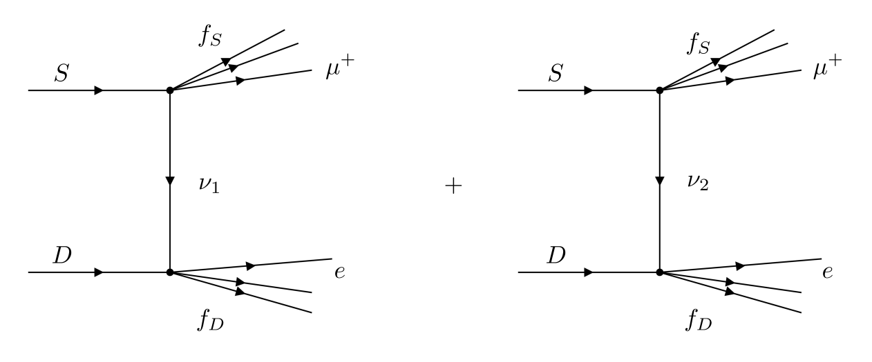
Figure 1: The physical process responsible for neutrino oscillations. Its amplitude is the sum of two diagrams with neutrinos $\nu_{1}$ and $\nu_{2}$ propagating in the $t$-channel.

It is well-appreciated by now Grimus:1996av ; Beuthe:2001rc ; Giunti:1993se ; Grimus:2019hlq ; Kiers:1997pe ; Naumov:2010um ; Naumov:2020yyv that establishing a connection between the scattering amplitude and the neutrino oscillation probability, requires introduction of wave packets for particles $S$ and $D$ in the initial state. Quite often wave packets for the final-state particles are also introduced but, as we will see, this is not necessary and we will not do that in what follows.

We describe initial states at the source and the detector as superpositions of momentum eigenstates

$$|S\rangle=\int[{\rm d}\vec{k}_{S}]\;\phi_{S}(\vec{k}_{S})\;|\vec{k}_{S}\rangle\,,\qquad|D\rangle=\int[{\rm d}\vec{k}_{D}]\;\phi_{D}(\vec{k}_{D})\;|\vec{k}_{D}\rangle\,,$$ (4)

where

$$[{\rm d}\vec{k}_{X}]=\frac{{\rm d}^{3}\vec{k}_{X}}{(2\pi)^{3/2}\sqrt{2E_{X}}}\,,\;\;\;\;\;X=S,D,$$ (5)

and $E_{X}=\sqrt{\vec{k}_{X}^{2}+m_{X}^{2}}$ is the energy of the particle with the momentum $\vec{k}_{X}$ and the mass $m_{X}$. We assume the standard relativistic normalization of states $|\vec{k}_{S,D}\rangle$, i.e.,

$$\langle\vec{k}_{X}^{\prime}|\vec{k}_{X}\rangle=2E_{X}(2\pi)^{3}\delta^{(3)}(\vec{k}_{X}-\vec{k}_{X}^{\prime})\,,$$ (6)

and

$$\int{\rm d}^{3}\vec{k}_{X}\;\phi_{X}(\vec{k}_{X})\;\phi^{*}_{X}(\vec{k})=1\,,\qquad X=S,D\,.$$ (7)

It follows that

$$\langle S|S\rangle=\langle D|D\rangle=1.$$ (8)

The $S$-matrix element for the process eq. 3 is given by

$$S_{if}=\int[{\rm d}\vec{k}_{S}][{\rm d}\vec{k}_{D}]\phi_{S}(\vec{k}_{S})\phi_{D}(\vec{k}_{D})(2\pi)^{4}\delta^{(4)}(k_{S}+k_{D}-P_{S}-P_{D})\mathcal{M}_{if}\,.$$ (9)

Then the differential transition probability $i\to f$ is obtained from the following equation:

$$\mathrm{d}W_{if}=|S_{if}|^{2}\;\mathrm{d}\nu_{f}\,,$$ (10)

where ${\rm d}\nu_{f}$ is the density of final states. It reads

$$\mathrm{d}\nu_{f}=\mathrm{d}\Phi_{S}\;\mathrm{d}\Phi_{D}\,,\qquad\mathrm{d}\Phi_{S}=\prod_{x\in S}\frac{\mathrm{d}^{3}p_{x}}{(2\pi)^{3}2E_{x}}\,,\qquad\mathrm{d}\Phi_{D}=\prod_{x\in D}\frac{\mathrm{d}^{3}p_{x}}{(2\pi)^{3}2E_{x}}\,,$$ (11)

where $x$ runs over all final-state particles, either in the source or in the detector. We find

$$\begin{split}\mathrm{d}W_{if}=&\int[{\rm d}\vec{k}_{S}][{\rm d}\vec{k}_{S}^{\prime}][{\rm d}\vec{k}_{D}][{\rm d}\vec{k}_{D}^{\prime}]\;\mathrm{d}\Phi_{S}\mathrm{d}\Phi_{D}\,\phi_{S}(\vec{k}_{S})\phi_{D}(\vec{k}_{D})\phi_{S}^{*}(\vec{k}^{\prime}_{S})\phi_{D}^{*}(\vec{k}^{\prime}_{D})\\ &\times(2\pi)^{4}\delta^{(4)}(k_{S}+k_{D}-P_{S}-P_{D})(2\pi)^{4}\delta^{(4)}(k^{\prime}_{S}+k^{\prime}_{D}-P_{S}-P_{D})\mathcal{M}_{if}\mathcal{M}^{\prime*}_{if}\,,\end{split}$$ (12)

where $\mathcal{M}^{\prime}_{if}$ indicates that this matrix element depends on the primed momenta.

To simplify this expression, we follow the approach described in refs. Ginzburg:1991mv ; Ginzburg:1991mw ; Kotkin:1992bj , but also introduce an important modification that is needed to describe the set-up of neutrino oscillation experiments. We start with an observation that for the description of a sequential process, where a neutrino is produced at the source, and then absorbed at the detector, it is useful to introduce the neutrino momenta

$$q=k_{S}-P_{S}=P_{D}-k_{D},\;\;\;q^{\prime}=k_{S}^{\prime}-P_{S}=P_{D}-k_{D}^{\prime}.$$ (13)

Then, we insert

$$1=\int{\rm d}^{4}q\delta^{(4)}(k_{S}-P_{S}-q)\int{\rm d}^{4}q^{\prime}\delta^{(4)}(k_{S}^{\prime}-P_{S}-q^{\prime}),$$ (14)

into eq. (12), rewrite delta-functions there separating them into “production” and “detection” ones, change variables to

$$Q=\frac{q+q^{\prime}}{2}\,,\quad\kappa=q-q^{\prime}\,,\qquad l_{X}=\frac{k_{X}+k^{\prime}_{X}}{2}\,,\quad\kappa_{X}=k_{X}-k^{\prime}_{X}\,,\quad(X=S,D),$$ (15)

and obtain

$$\begin{split}&\mathrm{d}W_{if}=\int[{\rm d}\vec{k}_{S}][{\rm d}\vec{k}_{S}^{\prime}][{\rm d}\vec{k}_{D}][{\rm d}\vec{k}_{D}^{\prime}]\;\mathrm{d}\Phi_{S}\mathrm{d}\Phi_{D}\,\phi_{S}(\vec{k}_{S})\phi_{D}(\vec{k}_{D})\phi_{S}^{*}(\vec{k}^{\prime}_{S})\phi_{D}^{*}(\vec{k}^{\prime}_{D})\mathcal{M}_{if}\mathcal{M}^{\prime*}_{if}\\ &\times{\rm d}^{4}\kappa{\rm d}^{4}Q\delta^{(4)}(\kappa_{S}-\kappa)\delta^{(4)}(\kappa_{D}+\kappa)(2\pi)^{4}\delta^{(4)}(l_{S}-P_{S}-Q)(2\pi)^{4}\delta^{(4)}(l_{D}-P_{D}+Q)\,,\end{split}$$ (16)

where we have also used $\mathrm{d}^{4}q\mathrm{d}^{4}q^{\prime}=\mathrm{d}^{4}Q\mathrm{d}^{4}\kappa$. Physically, $Q,l_{S},l_{D}$ correspond to mean four-momenta of the internal neutrino, the source and the detector particles, respectively, whereas $\kappa,\kappa_{S,D}$ describe the momentum differences in the interfering states. We emphasize again that final-state momenta of all particles are kept fixed.

We then write the energy part of the $\delta$-function involving $\kappa$’s in eq. 16 as integrals over “source” and “detector” times

$$(2\pi)^{2}\delta(\kappa^{0}_{S}-\kappa^{0})\delta(\kappa^{0}_{D}+\kappa^{0})=\int\mathrm{d}t_{S}\,e^{-i(\kappa^{0}_{S}-\kappa^{0})t_{S}}\int\mathrm{d}t_{D}\,e^{-i(\kappa^{0}_{D}+\kappa^{0})t_{D}}\,.$$ (17)

As recognized in refs. Ginzburg:1991mv ; Ginzburg:1991mw ; Kotkin:1992bj , a step leading to key simplifications in eq. (16), is the statistical averaging over the various quantum states described by the wave functions $\phi_{S}$ and $\phi_{D}$. This averaging produces time-dependent momentum-space density matrices

$$\langle\phi_{X}(\vec{k}_{X})\phi_{X}^{*}(\vec{k}^{\prime}_{X})e^{-i\kappa^{0}_{X}t_{X}}\rangle=\rho_{X}(\vec{k}_{X},\vec{k}^{\prime}_{X},t_{X}),$$ (18)

for $X=S,D$. Another crucial observation of refs. Ginzburg:1991mv ; Ginzburg:1991mw ; Kotkin:1992bj is the utility of the so-called Wigner function Case2008 , related to the density matrix through a particular Fourier transform

$$\rho_{X}(\vec{k}_{X},\vec{k}^{\prime}_{X},t_{X})=\int\mathrm{d}^{3}\vec{r}_{X}\,n_{X}(\vec{r}_{X},\vec{l}_{X},t_{X})e^{-i\vec{\kappa}_{X}\vec{r}_{X}},\,\qquad X=S,D\,.$$ (19)

Indeed, the classical limit of a Wigner function is the phase-space distribution of particles described by the relevant density matrix; in our case, these distributions are exactly what is needed to describe the source and the detector of neutrinos.

We note that eqs. (17, 18, 19) show important difference between discussion in refs. Ginzburg:1991mv ; Ginzburg:1991mw ; Kotkin:1992bj , which focused on collider processes, and the neutrino oscillations case which we want to describe here. In refs. Ginzburg:1991mv ; Ginzburg:1991mw ; Kotkin:1992bj , $\kappa^{0}$ was integrated out, and a single time-like variable was introduced $(2\pi)\delta(\kappa^{0}_{S}-\kappa^{0}_{D})=\int\mathrm{d}t\,e^{-i(\kappa^{0}_{S}-\kappa^{0}_{D})t}$. This implies that phase-space densities at both vertices are evaluated at the same value of $t$. In contrast, eq. 17 introduces two separate time variables for the source and detector, such that source and detector densities are evaluated at different times. This is important for properly describing retardation effects that are essential because sources and detectors in neutrino oscillation experiments can be separated by very large distances. Hence, as we will find below, relevant values of $t_{S}$ and $t_{D}$ will be determined by specific properties of the source and detector, as well as time required for a neutrino to propagate between them.

Physically, replacing the time components of the delta-functions with the time-dependent densities $n_{S}(t_{S})$ and $n_{D}(t_{D})$ corresponds to introducing energy non-conservation: energy will be conserved in the source/detector processes only within accuracy $\delta E_{X}\sim 1/\tau_{X}$, where $\tau_{X}$ is a characteristic time scale over which source or detector densities $n_{S,D}$ change. Different from collider experiment, in neutrino oscillation experiments the time structure of the source and the detector are unrelated and can be very different, making introduction of two, rather than one, times an important physically-motivated modification.

Returning to the calculation of the transition probability $\mathrm{d}W_{if}$ in eq. (12), we change the integration variables $\mathrm{d}^{3}\vec{k}_{X}\mathrm{d}^{3}\vec{k}^{\prime}_{X}=\mathrm{d}^{3}\vec{l}_{X}\mathrm{d}^{3}\vec{\kappa}_{X}$, $X=S,D$, and integrate over $\mathrm{d}^{3}\vec{\kappa}_{S}\mathrm{d}^{3}\vec{\kappa}_{D}$ finding $\vec{\kappa}=\vec{\kappa}_{S}=-\vec{\kappa}_{D}$. After collecting remaining terms, eq. 12 becomes

$$\begin{split}\mathrm{d}W_{if}=&\int\prod\limits_{x={S,D}}\frac{\mathrm{d}^{3}\vec{l}_{X}}{\sqrt{2E_{X}2E^{\prime}_{X}}}\;\mathrm{d}t_{X}\mathrm{d}^{3}\vec{r}_{X}\mathrm{d}^{3}n_{X}(\vec{r}_{X},\vec{l}_{X},t_{X})\,\mathrm{d}^{4}Q\mathrm{d}^{4}\kappa\;e^{-i\kappa_{\mu}x^{\mu}}\\ &\times\delta^{(4)}(l_{S}-P_{S}-Q)\delta^{(4)}(l_{D}-P_{D}+Q)\mathcal{M}_{if}\mathcal{M}^{\prime*}_{if}\,\mathrm{d}\Phi_{S}\mathrm{d}\Phi_{D},\end{split}$$ (20)

where $x^{\mu}=(t_{D}-t_{S},\vec{r}_{D}-\vec{r}_{S})$. We continue with the discussion of the matrix element and note that for processes that lead to neutrino oscillations, the neutrino in the $t$-channel should be close to its mass shell. It follows that the amplitude can be written in a factorised form

$$\mathcal{M}_{if}\approx-\sin\theta\cos\theta\,M_{S}\sum_{a=1,2}\frac{(-1)^{a}}{q^{2}-m_{a}^{2}+i\epsilon}M_{D}\,.$$ (21)

where, $\theta$ is the mixing angle, and $M_{S},M_{D}$ are the matrix elements for the production and detection processes of the massless on-shell neutrinos of the respective flavor, and the sum originates from the two diagrams with the two neutrino mass eigenstates in the $t$-channel. Neutrino masses are referred to as $m_{1,2}$. Another natural assumption is that the dependence of $M_{S,D}$ on the neutrino momenta is smooth enough, to neglect differences between $q$ and $q^{\prime}$ there and use $q\approx q^{\prime}\approx Q$. Then we obtain

$$\mathcal{M}_{if}\mathcal{M}^{\prime*}_{if}=\sin^{2}\theta\cos^{2}\theta\,|M_{S}|^{2}|M_{D}|^{2}\sum_{a,b=1,2}\frac{(-1)^{a}(-1)^{b}}{(q^{2}-m_{a}^{2}+i\epsilon)(q^{\prime 2}-m_{b}^{2}-i\epsilon)}\,.$$ (22)

We use eq. 15, to re-write neutrino momenta squared $q^{2}$ and $q^{\prime 2}$ in terms of $Q$ and $\kappa$ finding

$$\begin{split}q^{2}&=(Q+\kappa/2)^{2}\approx Q^{2}+Q\kappa+{\cal O}(\kappa^{2})\,,\\ q^{\prime 2}&=(Q-\kappa/2)^{2}\approx Q^{2}-Q\kappa+{\cal O}(\kappa^{2})\,.\end{split}$$ (23)

As we will see later, the magnitude of the vector $\kappa$ is determined by the macroscopic distance between source and detector. For this reason $\kappa/Q$ is tiny, and we can neglect terms of order $\kappa^{2}$ in what follows. The transition probability becomes

$$\begin{split}\mathrm{d}W_{if}&=\sin^{2}\theta\cos^{2}\theta\int\frac{\mathrm{d}^{4}Q}{(2\pi)^{4}}\\ &\times\mathrm{d}\Phi_{S}\int\frac{\mathrm{d}^{3}\vec{l}_{S}}{2E_{S}}\int\mathrm{d}t_{S}\mathrm{d}^{3}\vec{r}_{S}\,n_{S}(\vec{r}_{S},\vec{l}_{S},t_{S})\,(2\pi)^{4}\delta^{(4)}(l_{S}-P_{S}-Q)\,|M_{S}|^{2}\\ &\times\mathrm{d}\Phi_{D}\int\frac{\mathrm{d}^{3}\vec{l}_{D}}{2E_{D}}\int\mathrm{d}t_{D}\mathrm{d}^{3}\vec{r}_{D}\,n_{D}(\vec{r}_{D},\vec{l}_{D},t_{D})\,(2\pi)^{4}\delta^{(4)}(l_{D}-P_{D}+Q)\,|M_{D}|^{2}\\ &\times\int\frac{\mathrm{d}^{4}\kappa}{(2\pi)^{4}}\,e^{-i\kappa x}\sum_{a,b=1,2}\frac{(-1)^{a}(-1)^{b}}{(Q^{2}+Q\kappa-m_{a}^{2}+i\epsilon)(Q^{2}-Q\kappa-m_{b}^{2}-i\epsilon)}\,,\end{split}$$ (24)

where we replaced $E_{S,D}$ and $E_{S,D}^{\prime}$ with $E_{S,D}(\vec{l}_{S,D})$.

The main contribution to the above integral comes from the integration region where $Q^{2}\sim m_{1,2}^{2}$. For such $Q^{2}$, we can re-write the integration $\mathrm{d}^{4}Q$ in such a way that the integration over the neutrino “mass” $Q^{2}$ and its phase-space element ${\rm d}^{3}\vec{Q}/(2Q_{0}(2\pi)^{3})$ with $Q_{0}=\sqrt{\vec{Q}^{2}+Q^{2}}$ appear, by changing integration variables $\mathrm{d}Q^{0}\to\mathrm{d}Q^{2}$. Furthermore, making the natural assumption that neutrinos produced in the source are ultra-relativistic, we can drop $Q^{2}$ in the expression for $Q_{0}$. Then, eq. 24 simplifies as follows

$$\begin{split}\mathrm{d}W_{if}&=\sin^{2}\theta\cos^{2}\theta\int\frac{\mathrm{d}Q^{2}}{2\pi}\int\frac{\mathrm{d}^{3}\vec{l}_{S}}{2E_{S}}\int\mathrm{d}t_{S}\;\mathrm{d}^{3}\vec{r}_{S}\,n_{S}(\vec{r}_{S},\vec{l}_{S},t_{S})\,\\ &\times(2\pi)^{4}\delta^{(4)}(l_{S}-P_{S}-Q)\,|M_{S}|^{2}\mathrm{d}\Phi_{S}\frac{\mathrm{d}^{3}\vec{Q}}{(2\pi)^{3}2|\vec{Q}|}\\ &\times\int\frac{\mathrm{d}^{3}\vec{l}_{D}}{2E_{D}}\int\mathrm{d}t_{D}\;\mathrm{d}^{3}\vec{r}_{D}\,n_{D}(\vec{r}_{D},\vec{l}_{D},t_{D})\,(2\pi)^{4}\delta^{(4)}(l_{D}-P_{D}+Q)\,|M_{D}|^{2}\mathrm{d}\Phi_{D}\\ &\times\int\frac{\mathrm{d}^{4}\kappa}{(2\pi)^{4}}\,e^{-i\kappa x}\sum_{a,b=1,2}\frac{(-1)^{a}(-1)^{b}}{(Q^{2}+Q\kappa-m_{a}^{2}+i\epsilon)(Q^{2}-Q\kappa-m_{b}^{2}-i\epsilon)}\,.\end{split}$$ (25)

As we already mentioned, neutrinos are nearly on-shell, which implies that in $Q\kappa$ terms, we replace $Q_{0}$ with $|\vec{Q}|$. This is accurate up to $\mathcal{O}(\kappa m_{\nu})$ terms, which we neglect. Then the integral over $Q^{2}$ is only important for the last line in eq. 25. Hence, we define a function

$$I(x_{\mu},Q^{\mu})=\int\frac{{\rm d}Q^{2}}{2\pi}\;\frac{\mathrm{d}^{4}\kappa}{(2\pi)^{4}}\,e^{-i\kappa x}\sum_{a,b=1,2}\frac{(-1)^{a}(-1)^{b}}{(Q^{2}+Q\kappa-m_{a}^{2}+i\epsilon)(Q^{2}-Q\kappa-m_{b}^{2}-i\epsilon)}\,,$$ (26)

which, as we will see shortly, provides the neutrino oscillation probability. To compute this function, we integrate over $Q^{2}$ using the residue theorem and find

$$I\equiv\frac{i}{|\vec{Q}|}\int\frac{\mathrm{d}^{4}\kappa}{(2\pi)^{4}}\,e^{-i\kappa x}\left[\frac{1}{n_{\nu}\kappa+i\epsilon}-\frac{1}{2}\left(\frac{1}{n_{\nu}\kappa+2L^{-1}_{\rm osc}+i\epsilon}+\frac{1}{n_{\nu}\kappa-2L_{\rm osc}^{-1}+i\epsilon}\right)\right].$$ (27)

where the neutrino oscillation length is defined as

$$L_{\rm osc}=\frac{4|\vec{Q}|}{\Delta m^{2}},$$ (28)

$\Delta m^{2}\equiv m^{2}_{2}-m^{2}_{1}$, and $n_{\nu}=(1,\vec{e}_{\nu})$ is the four-vector that describes the world-line of a propagating ultra-relativistic neutrino.

To complete the integration in eq. 27, we use the identity

$$\frac{i}{A+i\epsilon}\equiv\int\limits_{0}^{\infty}\mathrm{d}\tau\,e^{iA\tau},$$ (29)

integrate over $\kappa$, and find

$$I=\frac{2}{|\vec{Q}|}\int\limits_{0}^{\infty}\mathrm{d}\tau\,\delta^{(4)}(x-\tau n_{\nu})\sin^{2}\left(\frac{\tau}{L_{\rm osc}}\right)\,.$$ (30)

To proceed further, we use the definition of the four-vector $x^{\mu}=(t_{D}-t_{S},\vec{r}_{D}-\vec{r}_{S})$, and explicitly write the delta-function by separating components of $\vec{x}$ into parallel and orthogonal ones relative to the neutrino momentum. We obtain

$$\delta^{(4)}(x-\tau n_{\nu})=\delta(t_{D}-t_{S}-\tau)\,\delta(r_{||}-\tau)\,\delta^{(2)}(\vec{r}_{\perp})\,,$$ (31)

where $\vec{r}=\vec{r}_{D}-\vec{r}_{S}$, $r_{||}=\vec{r}\cdot\vec{e}_{\nu}$ and $\vec{r}_{\perp}\cdot\vec{e}_{\nu}=0$. Integrating over $\tau$, we find

$$I=\frac{2}{|\vec{Q}|}\delta(t_{D}-t_{S}-r_{\parallel})\,\delta^{(2)}(\vec{r}_{\perp})\,\Theta(r_{||})\sin^{2}\left(\frac{r_{||}}{L_{\rm osc}}\right)\,.$$ (32)

Using this result in eq. 25, integrating over detection time $t_{D}$, and replacing the neutrino momentum $Q$ with $p_{\nu}=E_{\nu}(1,\vec{e}_{\nu})$ for the sake of clarity, we find

$$\begin{split}\mathrm{d}W_{if}&=\int\mathrm{d}t_{S}\;\mathrm{d}^{3}\vec{l}_{S}\mathrm{d}^{3}\vec{r}_{S}\,n_{S}(\vec{r}_{S},\vec{l}_{S},t_{S})\mathrm{d}^{3}\vec{l}_{D}\mathrm{d}^{3}\vec{r}_{D}\,n_{D}(\vec{r}_{D},\vec{l}_{D},t_{S}+(\vec{r}_{D}-\vec{r}_{S})\cdot\vec{e}_{\nu})\\ &\times\frac{1}{2E_{S}}(2\pi)^{4}\delta^{(4)}(l_{S}-P_{S}-p_{\nu})\,|M_{S}|^{2}\;\mathrm{d}\Phi_{S}\frac{\mathrm{d}^{3}\vec{p}_{\nu}}{(2\pi)^{3}2E_{\nu}}\\ &\times\,\frac{1}{2E_{\nu}}\frac{1}{2E_{D}}\,(2\pi)^{4}\delta^{(4)}(l_{D}-P_{D}+p_{\nu})\,|M_{D}|^{2}\mathrm{d}\Phi_{D}\\ &\times\delta^{(2)}(\vec{r}_{D,\perp}-\vec{r}_{S,\perp})\,\Theta[(\vec{r}_{D}-\vec{r}_{S})\cdot\vec{e}_{\nu}]\,\sin^{2}2\theta\;\sin^{2}\left(\frac{(\vec{r}_{D}-\vec{r}_{S})\cdot\vec{e}_{\nu}}{L_{\rm osc}}\right)\,.\end{split}$$ (33)

We can easily identify the physical meaning of several contributions to the above equation. The first one is the standard neutrino oscillation probability

$$P_{\rm osc}(\vec{r}_{D},\vec{r}_{S},\vec{e}_{\nu})=\sin^{2}2\theta\sin^{2}\left(\frac{(\vec{r}_{D}-\vec{r}_{S})\cdot\vec{e}_{\nu}}{L_{\rm osc}}\right)\,.$$ (34)

We note that, when this expression is used in eq. (33) together with the transverse delta-function, we can replace $(\vec{r}_{D}-\vec{r}_{S})\cdot\vec{e}_{\nu}=|\vec{r}_{D}-\vec{r}_{S}|$.

The second identifiable contribution in eq. 33 is the differential decay rate of the source particle in the laboratory frame

$$\mathrm{d}\Gamma_{S}=\frac{1}{2E_{S}}(2\pi)^{4}\delta^{(4)}(l_{S}-P_{S}-p_{\nu})\,|M_{S}|^{2}\,\mathrm{d}\Phi_{S\nu}.$$ (35)

We note that

$$\mathrm{d}\Phi_{S\nu}=\frac{\mathrm{d}^{3}p_{\nu}}{(2\pi)^{3}2E_{\nu}}\,\mathrm{d}\Phi_{S}\,,$$ (36)

is the phase space element for the final state of the process $S\to f_{S}+\nu$.

Third, the quantity in the third line of eq. 33 is related to the differential cross section of the process $D+\nu\to f_{D}$

$$(1-\vec{e}_{\nu}\cdot\vec{\beta}_{D})\;\mathrm{d}\sigma_{D\nu}=\frac{1}{2E_{D}2E_{\nu}}\mathrm{d}\Phi_{D}(2\pi)^{4}\delta^{(4)}(l_{D}-P_{D}+p_{\nu})\,|M_{D}|^{2}\,,$$ (37)

where $\vec{\beta}_{D}$ is the velocity of the detector particle $D$.

Finally, it is possible to write the transversal delta-function as

$$\delta^{(2)}(\vec{r}_{\perp})=\frac{1}{r^{2}}\,\left(\delta^{(2)}(\vec{e}_{r}-\vec{e}_{\nu})+\delta^{(2)}(\vec{e}_{r}+\vec{e}_{\nu})\right),$$ (38)

where $\vec{e}_{r}=\vec{r}/r$ and the delta-functions on the right-hand side are defined as follows

$$\int{\rm d}\Omega_{\vec{r}}\;\delta^{(2)}(\vec{e}_{r}-\vec{e}_{\nu})f(\vec{r})=f(r\vec{e}_{\nu}).$$ (39)

Equation 38 leads to the inverse distance-squared dependence of the neutrino flux at the detector. Hence, the transition probability in eq. 33 can be written as follows

$$\begin{split}\mathrm{d}W_{if}&=\int\mathrm{d}^{3}\vec{p}_{\nu}\,\int\mathrm{d}t_{S}\mathrm{d}^{3}\vec{l}_{S}\mathrm{d}^{3}\vec{r}_{S}\,n_{S}(\vec{r}_{S},\vec{l}_{S},t_{S})\,\frac{\mathrm{d}\Gamma_{S}}{\mathrm{d}^{3}\vec{p}_{\nu}}\\ &\times\int\mathrm{d}r\,\mathrm{d}^{3}\vec{l}_{D}\,n_{D}(\vec{r}_{S}+r\vec{e}_{\nu},\vec{l}_{D},t_{S}+r)\,\mathrm{d}\sigma_{D\nu}\;P_{\rm osc}(r)\,,\end{split}$$ (40)

where we have assumed that the detector particle is non-relativistic and replaced the factor $1-\vec{e}_{\nu}\cdot\vec{\beta}_{D}$ in eq. 37 with one. Furthermore, we have changed the integration variables from $\mathrm{d}^{3}\vec{r}_{D}\to\mathrm{d}^{3}\vec{r}$, switched to polar coordinates, and used eq. 39 for the angular integration. The factor $1/r^{2}$ from eq. 38 cancels with the $r^{2}$ from the volume element in spherical coordinates.

3 Impact of the source and detector densities and the decoherence effects

Equation 40 offers a very suggestive expression, where the product of the decay rate for the source particle multiplied with the oscillation probability and the detection cross section is convoluted with the phase-space densities of source and detector particles. This convolution impacts the possibility to observe neutrino oscillations as we will now explain. In addition to these classical averaging effects, the derivation in the previous section allows to identify assumptions leading to the standard oscillation probability, and quantify conditions, under which these assumptions hold. Once they are violated, decoherence effects will modify the oscillation pattern. We will comment on this at the end of this section, and show that these effects are parametrically equivalent to the classical averaging suggested by eq. 40.

In order to study this effect, we will consider a toy model, assuming that the source and detector phase-space densities have a Gaussian shape in space, momentum and time

$$n_{X}(\vec{r}_{X},\vec{l}_{X},t_{X})\propto\exp\left[-\frac{1}{2}\left(\frac{\vec{r}_{X}-\vec{L}_{X}}{\delta_{X}}\right)^{2}-\frac{1}{2}\left(\frac{\vec{l}_{X}-\vec{\sf l}_{X}}{\sigma_{X}}\right)^{2}-\frac{1}{2}\left(\frac{t_{X}-T_{X}}{\tau_{X}}\right)^{2}\right]\,,$$ (41)

for $X=S,D$, with the mean locations $\vec{L}_{S,D}$, mean momenta $\vec{\sf l}_{S,D}$, and mean times $T_{S,D}$. For simplicity we assume the distributions to be isotropic. Quantum mechanics requires

$$\delta_{X}\sigma_{X}>\frac{1}{2}\,.$$ (42)

The time spreads $\tau_{S,D}$ represent typical time scales, over which the source and detector change. As mentioned above, this implies that energy is conserved in the corresponding processes only approximately, up to $\delta E_{X}\sim 1/\tau_{X}$ ($X=S,D$). In the next section we will consider a specific realisation of such a situation – the time dependence induced by the decay of the source particle.

Let us first consider the consequences of the spatial and time localizations. As the decay rate and detection cross section do not depend on space and time, only the delta-functions and the oscillation probability are folded with the corresponding Gaussians in eq. (41). Substituting these densities into eq. 40, we find that the following integral is needed

$$\int\limits_{0}^{\infty}\mathrm{d}r\int\mathrm{d}t_{S}\;\mathrm{d}^{3}\vec{r}_{S}e^{-\frac{1}{2}\left(\frac{\vec{r}_{S}-\vec{L}_{S}}{\delta_{S}}\right)^{2}}e^{-\frac{1}{2}\left(\frac{t_{S}-T_{S}}{\tau_{S}}\right)^{2}}e^{-\frac{1}{2}\left(\frac{\vec{r}_{S}+r\vec{e}_{\nu}-\vec{L}_{D}}{\delta_{D}}\right)^{2}}e^{-\frac{1}{2}\left(\frac{t_{S}+r-T_{S}}{\tau_{D}}\right)^{2}}P_{\rm osc}(r).$$ (43)

To compute it, we express the sine function that appears in the neutrino oscillation probability as a linear combination of complex-valued exponential functions, extend the integral over $r$ to $-\infty$, which allows us to get leading contributions without having to deal with the error functions, and find the following expression for the “smeared” oscillation probability

$$\begin{split}P_{\rm osc}&=\frac{1}{2}\sin^{2}2\theta\exp\left[-\frac{(\vec{L}_{D\perp}-\vec{L}_{S\perp})^{2}}{2\delta^{2}}\right]\exp\left[-\frac{1}{2}\frac{(L-T)^{2}}{\tau^{2}+\delta^{2}}\right]\\ &\times\left[1-\exp\left(-\frac{1}{2}\frac{\tau^{2}\delta^{2}}{\tau^{2}+\delta^{2}}\Delta^{2}\right)\cos\left(\Delta\frac{\tau^{2}L+\delta^{2}T}{\tau^{2}+\delta^{2}}\right)\right]\,,\end{split}$$ (44)

where

$$\Delta\equiv\frac{\Delta m^{2}}{2E_{\nu}}=\frac{2}{L_{\rm osc}}\,,$$ (45)

and

$$\begin{split}&\tau^{2}\equiv\tau_{D}^{2}+\tau_{S}^{2}\,,\quad\delta^{2}\equiv\delta_{D}^{2}+\delta_{S}^{2}\,,\quad L\equiv(\vec{L}_{D}-\vec{L}_{S})\cdot\vec{e}_{\nu},\,\quad T\equiv T_{D}-T_{S}\,.\end{split}$$ (46)

The exponential involving $\vec{L}_{S,D\perp}$ constrains the direction of $\vec{p}_{\nu}$ within an opening angle of $\lesssim\delta/L$, whereas the second exponential in the first line constrains the mean distances $T\approx L$ within $\sqrt{\tau^{2}+\delta^{2}}$. The exponential in the second line gives the decoherence suppression of oscillations. It is dominated by the smaller spread of $\tau$ and $\delta$, i.e., oscillations are damped if $\rm{min}(\tau,\delta)\Delta\gtrsim 1$.

The cosine term in eq. (44) describes the modified oscillation phase. If $\tau\gg\delta$ ($\tau\ll\delta$) oscillations happen in space (time). Hence, for $\tau\lesssim\delta$ we would predict deviations from the canonical oscillations in space.

The limit $\tau\to\infty$, that can be realized by taking $\tau_{D}\to\infty$, corresponds to the case of a stationary detector. Apart from the constraint in the transverse direction, we obtain in this case

$$P_{\rm osc} =\frac{1}{2}\sin^{2}2\theta\left[1-\exp\left(-\frac{\delta^{2}\Delta^{2}}{2}\right)\cos\left(\Delta L\right)\right],\qquad(\tau\gg\delta)\,.$$ (47)

This formula corresponds to the usual localization condition: observability of oscillations requires that processes occurring at the source and the detector are much better localized than the neutrino oscillation length, $\delta\ll L_{\rm osc}$. Consider, for example, a non-relativistic detector particle and assume that it is localized within a distance $\delta_{D}\sim D$, where $D$ is a typical inter-atomic or inter-molecular distance. If the detector particle moves non-relativistically with velocity $\beta_{D}\ll 1$, it will be localized in time with $\tau_{D}\sim D/\beta_{D}\gg\delta_{D}$. Hence, if for the source we have $\tau_{S}\gtrsim\delta_{S}$, we recover the “stationary detector” case for non-relativistic detector particles. Another example of $\tau_{D}\to\infty$ would be a detector particle in a bound state with fixed energy eigenvalue.

There is an interesting consequence of the assumption that the detector is stationary. Indeed, stationary detector implies that the phase-space density $n_{D}$ does not depend on time. Then the $\mathrm{d}t_{D}$ integral in eq. 24 gives a delta-function $\delta(\kappa^{0})$ and the $\mathrm{d}\kappa^{0}$ integral sets $\kappa^{0}=0$, which means that interfering neutrinos have identical energies Grimus:1996av ; Grimus:1998uh . In the approach of Krueger:2023skk ; Akhmedov:2010ms this is obtained by integrating over an unobservable neutrino propagation time (which resembles somewhat the $\mathrm{d}t_{D}$ integration in our approach). The assumption of a completely stationary detector has been relaxed in Grimus:2019hlq .

Moving to the momentum integrals, we can perform the $\mathrm{d}^{3}\vec{l}_{S,D}$ integrals using spatial parts of the delta-functions in eqs. 35 and 37, such that the Gaussian factors become

$$\exp\left[-\frac{(\vec{P}_{S}+\vec{p}_{\nu}-\bar{\sf l}_{S})^{2}}{2\sigma_{S}^{2}}-\frac{(\vec{P}_{D}-\vec{p}_{\nu}-\bar{\sf l}_{D})^{2}}{2\sigma_{D}^{2}}\right]\,.$$ (48)

These factors will have to be integrated further over $\mathrm{d}^{3}\vec{p}_{\nu}$. The angular part of this integral will be constrained by the Gaussian factor in eq. 44 which involves transverse directions. Then we are left with an integral of the type

$$\int\mathrm{d}E_{\nu}\,h(E_{\nu})e^{-g(E_{\nu})\pm i\Delta L}\,,$$ (49)

where $h(E_{\nu})$ is a sufficiently smooth function of $E_{\nu}$ and $g(E_{\nu})$ is a quadratic function in $E_{\nu}$ with

$$g^{\prime\prime}(E_{\nu})=\frac{1}{\sigma_{S}^{2}}+\frac{1}{\sigma_{D}^{2}}\equiv\frac{1}{\sigma^{2}}\,.$$ (50)

Applying the usual method (see e.g., Beuthe:2001rc , or Appendix A of Krueger:2023skk ), we find that this integration leads to an additional damping factor in eq. 44 such that the overall decoherence factor in front of the interference term becomes

$$\begin{split}&\exp\left[-\frac{1}{2}\left(\bar{\Delta}L\frac{\sigma}{\bar{E}_{\nu}}\right)^{2}\right]\exp\left(-\frac{1}{2}\frac{\tau^{2}\delta^{2}}{\tau^{2}+\delta^{2}}\bar{\Delta}^{2}\right)\quad\to\quad\\ &\exp\left[-\frac{1}{2}\left(\frac{\Delta m^{2}L\sigma}{2\bar{E}_{\nu}^{2}}\right)^{2}\right]\exp\left[-\frac{1}{2}\left(\frac{\Delta m^{2}\delta}{2\bar{E}_{\nu}}\right)^{2}\right],\qquad(\tau\gg\delta)\,,\end{split}$$ (51)

where $\bar{E}_{\nu}$ is the neutrino energy that minimizes $g(E_{\nu})$. Hence, within the toy Gaussian model, we recover the usual damping factors due to momentum and spatial localizations. Taking into account the fundamental uncertainty relation eq. 42, we see that oscillations would disappear, either for $\sigma\to 0$ or $\delta\to 0$, that is, intrinsic delocalisation both in space and momentum are required, as illustrated in fig. 2.

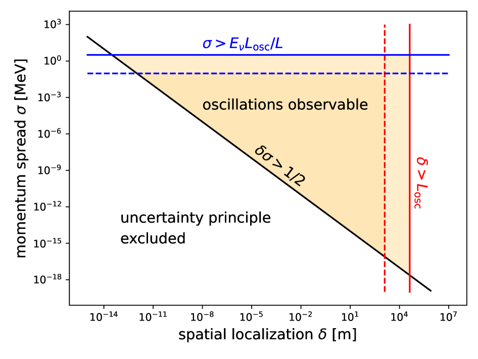
Figure 2: Values of spatial and momentum spreads required for the observability of oscillations (shaded region) from the coherence conditions implied by eq. 51 (red and blue lines) and the uncertainty principle (black line). For illustration purposes we adopt parameters relevant for the JUNO reactor experiment: $E_{\nu}=4$ MeV, $L=53$ km. Solid (dashed) lines refer to $\Delta m^{2}=7.5\times 10^{-5}\,(2.5\times 10^{-3})$ eV².

Let us now discuss decoherence effects related to the violation of some assumptions we adopted in section 2 to derive the oscillation probability. A crucial assumption in this derivation was the approximation that integrations over the neutrino invariant mass $Q^{2}$ and the 4-vector $\kappa$ in eq. 25 can be performed independently of the remaining terms in the integrand. While this assumption is natural, deviations from it lead to corrections to the derived formula and the pattern of neutrino oscillations will be affected.

Terms in the integrand in eq. (25) that one may consider include the matrix elements squared for the production and detection processes, the respective phase spaces, and the distribution functions $n_{S,D}(\vec{r},\vec{l},t)$ of source and detector particles. For example, in our approach, decoherence may occur if e.g. products of these quantities evaluated at the poles of two different neutrino propagators, $Q^{2}=m^{2}_{1}$ and $Q^{2}=m_{2}^{2}$, are so different from each other, that these differences cannot be ignored.

To provide an example, we will focus on the dependence of the distribution functions $n_{X}(\vec{r}_{X},\vec{l}_{X},t_{X})$ ($X=S,D$) on the momenta $\vec{l}_{X}$. To be specific we consider the source particle $X=S$, but the discussion is fully analogous for the detector. Since the main contribution to the integral over $Q^{2}$ comes from poles of the neutrino propagators in the two diagrams in fig. 1, and since we keep momenta of final state particles fixed, the momentum of the decaying particle $S$ will be different in the two cases. Starting from the equation

$$(l_{S_{1,2}}-P_{S})^{2}=m_{1,2}^{2},$$ (52)

and writing $l_{S_{1}}=(E_{S_{1}},\vec{l}_{S})$ and $l_{S_{2}}=(E_{S_{2}},\vec{l}_{S}+\delta\vec{l}_{S})$, it is easy to derive an estimate of the momentum differences between the residues for the two neutrino propagators

$$|\delta\vec{l}_{S}|\sim\frac{\Delta m^{2}}{|\vec{Q}|}\sim\frac{1}{L_{\rm osc}}\,.$$ (53)

The standard pattern of neutrino oscillations is obtained if the difference between distributions computed at $\vec{l}_{S}$ and $\vec{l}_{S}+\delta\vec{l}_{S}$ can be neglected

$$|n_{S}(\vec{r}_{S},\vec{l}_{S}+\delta\vec{l}_{S},t_{S})-n_{S}(\vec{r}_{S},\vec{l}_{S},t_{S})|\ll n_{S}(\vec{r}_{S},\vec{l}_{S},t_{S})\,.$$ (54)

Expanding the left-hand side of eq. 54 in $\delta\vec{l}_{S}$, we find

$$\frac{\partial n_{S}(\vec{r}_{S},\vec{l}_{S},t_{S})}{\partial\vec{l}_{S}}\;\delta\vec{l}_{S}\sim\left|\frac{\partial n_{S}(\vec{r}_{S},\vec{l}_{S},t_{S})}{\partial\vec{l}_{S}}\right|\;L_{\rm osc}^{-1}\ll n_{S}(\vec{r}_{S},\vec{l}_{S},t_{S})\,.$$ (55)

We estimate the derivative of the density using the inverse momentum spread $1/\sigma_{S}$ to arrive at the condition

$$\frac{1}{\sigma_{S}L_{\rm osc}}\ll 1\,.$$ (56)

This can be compared to the localisation condition $\delta\ll L_{\rm osc}$, see eq. 47. Together with the uncertainty relation eq. 42 we see that

$$\frac{1}{\sigma_{X}L_{\rm osc}}<\frac{2\delta_{X}}{L_{\rm osc}}\ll 1\qquad(X=S,D)\,,$$ (57)

where we generalized to source and detector. We see that the localization condition derived above by the classical averaging of the oscillation probability implies that the approximations adopted to perform the integrations in our derivation are automatically satisfied. This is another example of the fact that classical averaging and intrinsic quantum-mechanical decoherence effects are indistinguishable Kiers:1995zj ; Stodolsky:1998tc ; Ohlsson:2000mj ; Krueger:2023skk .

4 Effects of the decaying particle in the neutrino source

4.1 Derivation

We now extend the discussion in section 2 and consider the case when the neutrino in the source is produced by a decaying particle $R$, see refs. Grimus:1999ra ; Akhmedov:2010ms ; Grimus:2019hlq for earlier discussions of this problem. This particle is produced in a process $1+2\to R+f_{R}$, where $f_{R}$ is a final state with fixed momentum $P_{f_{R}}$. The resonance $R$ decays producing internal $t$-channel neutrino, $R\to\nu+f_{S}$.

We note that in addition to the academic interest, the discussion of a resonance is useful for understanding a set up where neutrinos are produced in decays of relativistic pions in a collimated beam, or for reactor neutrinos, where the resonance is a $\beta$-decaying nucleus produced in the fission of a mother nucleus.

The overall process is now $1+2+3\to f_{R}+f_{S}+f_{D}$, where we gave the detector particle $D$ a label $3$ for notational convenience. The $S$-matrix element of the total process is

$$S_{if}=\int\prod_{i=1}^{3}[\mathrm{d}\vec{k}_{i}]\;\phi_{i}(\vec{k}_{i})(2\pi)^{4}\delta^{(4)}(k_{123}-P_{f_{R}}-P_{S}-P_{D})A(k_{1},k_{2})W(q_{R})\mathcal{M}_{if}\,,$$ (58)

where $A$ is the amplitude of the process $1+2\to R+f_{R}$,

$$W(q_{R})=\frac{1}{q_{R}^{2}-M^{2}+iM\Gamma}$$ (59)

is the Breit-Wigner propagator, $q_{R}=k_{12}-P_{f_{R}}$ and $\mathcal{M}_{if}$ is the amplitude for the process $R+D\to f_{S}+f_{D}$. We use the short-hand notations $k_{12}$, $k_{123}$ to denote sums over the corresponding momenta. Furthermore, we assume that momenta $k_{1,2}$ are such that the on-shell production of the resonance $R$ is possible, i.e. that the condition $(k_{12}-P_{fR})^{2}=M^{2}$ is kinematically accessible.

To compute the probability of the process $1+2+3\to f_{R}+f_{S}+f_{D}$, we square the amplitude $S_{fi}$. Upon doing this, similar to the discussion in Section 2, we obtain two delta-functions, one with the argument $k_{123}-P_{f_{R}}-P_{S}-P_{D}$ and another one with the argument $k^{\prime}_{123}-P_{f_{R}}-P_{S}-P_{D}$. Following the discussion in Section 2, we rewrite these $\delta$-functions by introducing momenta for the resonance $R$ and the $t$-channel neutrino

$$\begin{split}&\delta^{(4)}(k_{123}-P_{fR}-P_{S}-P_{D})=\\ &\int\mathrm{d}^{4}q_{R}\mathrm{d}^{4}q_{\nu}\,\delta^{(4)}(k_{12}-q_{R}-P_{fR})\delta^{(4)}(q_{R}-q_{\nu}-P_{S})\delta^{(4)}(k_{3}+q_{\nu}-P_{D})\,.\end{split}$$ (60)

We do the same with the “primed” momenta and then move on to two average four-momenta and their differences, similar to what is done in eq. 15

$$\begin{split}&Q_{R}=\frac{q_{R}+q_{R}^{\prime}}{2},\;\;\;\kappa_{R}=q_{R}-q_{R}^{\prime}\,,\\ &Q\;\;=\frac{q_{\nu}+q_{\nu}^{\prime}}{2},\;\;\;\;\;\kappa\;\;=q_{\nu}-q_{\nu}^{\prime}\,.\end{split}$$ (61)

The product of two delta-functions that appears in $\mathrm{d}W_{if}$ becomes

$$\begin{split}\int\mathrm{d}^{4}Q_{R}\mathrm{d}^{4}Q\mathrm{d}^{4}\kappa_{R}\mathrm{d}^{4}\kappa\,&\delta^{(4)}(l_{12}-Q_{R}-P_{fR})\delta^{(4)}(Q_{R}-Q-P_{S})\delta^{(4)}(l_{3}+Q-P_{D})\\ &\times\delta^{(4)}(\kappa_{12}-\kappa_{R})\delta^{(4)}(\kappa_{R}-\kappa)\delta^{(4)}(\kappa_{3}+\kappa_{\nu})\,.\end{split}$$ (62)

The transition probability $\mathrm{d}W_{if}$ can be calculated following the discussion in Section 2. We provide the details of this calculation in appendix A. If follows from that discussion that the integral $I$ in eq. (26) – a quantity that is directly related to the neutrino oscillation probability – is generalized to

$$\begin{split}I_{R}=2\Gamma M\;\int&\frac{{\rm d}Q_{R}^{2}}{2\pi}\frac{{\rm d}Q^{2}}{2\pi}\frac{{\rm d}^{4}\kappa}{(2\pi)^{4}}e^{-i\kappa_{\mu}x^{\mu}}\,W\left(Q_{R}+\frac{\kappa}{2}\right)W^{*}\left(Q_{R}-\frac{\kappa}{2}\right)\\ &\times\sum_{a,b=1,2}\frac{(-1)^{a}(-1)^{b}}{(Q^{2}+Q\kappa-m_{a}^{2}+i\epsilon)(Q^{2}-Q\kappa-m_{b}^{2}-i\epsilon)}\,,\end{split}$$ (63)

where $x^{\mu}=(t_{D}-t_{S},\vec{r}_{D}-\vec{r}_{S})$. We note that $t_{S}$ and $\vec{r}_{S}$ in this case refer to the space-time point where particles $1$ and $2$ collide to produce a resonance $R$, rather than the space-time point where the neutrino was produced.

Equation (63) describes two effects – the impact of the finite lifetime of a resonance on the neutrino oscillation probability, and the effect of the smearing of the neutrino energy caused by the resonance off-shellness. Both of these effects can be accounted for at once but, for the sake of simplicity we will focus on the former and then briefly comment on the latter.

To describe the impact of the resonance finite lifetime, we assume that the neutrino energy is independent of the resonance off-shellness. This allows us to integrate over $Q_{R}^{2}$ in eq. (63). The Breit-Wigner terms have poles at

$$Q_{R}^{2}=M^{2}\pm\kappa Q_{R}\pm iM\Gamma\,,$$ (64)

and, applying the residue theorem, we find

$$\int\frac{{\rm d}Q_{R}^{2}}{2\pi}\,W\left(Q_{R}+\frac{\kappa}{2}\right)W^{*}\left(Q_{R}-\frac{\kappa}{2}\right)=\frac{1}{2Q_{R}^{0}}\;\frac{i}{\kappa\beta_{R}+i\Gamma/\gamma_{R}}\,,$$ (65)

where $\beta_{R}^{\mu}=(1,\vec{\beta}_{R})$ is the four-velocity of the resonance and $\gamma_{R}=Q_{R}^{0}/M$ is the resonance $\gamma$-factor. To perform subsequent integrations over $Q^{2}$ and $\kappa$, we write

$$\frac{i}{\kappa\beta_{R}+i\Gamma/\gamma_{R}}=\int\limits_{0}^{\infty}{\rm d}t_{R}\;e^{-t_{R}/\tau_{R}}\;e^{i\kappa\beta_{R}t_{R}}\,,$$ (66)

where $\tau_{R}=\gamma_{R}/\Gamma$ is the lifetime of the resonance in the laboratory frame. Using this representation in eq. 63, we observe that the integration over $Q^{2}$ and $\kappa$ can be performed following what was discussed earlier in section 2. We obtain

$$I_{R}=\frac{1}{\tau_{R}}\int\limits_{0}^{\infty}{\rm d}t_{R}\;e^{-t_{R}/\tau_{R}}\;I(x_{D}^{\mu}-x_{S}^{\mu}-\beta_{R}^{\mu}t_{R},Q)\,,$$ (67)

where $I$ is given in eq. 32. Equation 67 has a clear physical interpretation, namely the smearing of the distance, over which oscillations are observed, over the finite life-time of the resonance. To quantify this effect, we consider the following integral

$$I_{R} =\frac{2}{\tau_{R}|\vec{Q}|}\int\limits_{0}^{\infty}{\rm d}t_{R}\,e^{-t_{R}/\tau_{R}}\sin^{2}\frac{(r_{||}-\beta_{R||}t_{R})}{L_{\rm osc}}\,,$$ (68)

which follows from eq. 67 if the transverse $\delta$-functions and their dependence on $\vec{\beta}_{R}$ are neglected. As in section 2, we use the notation $r_{||}=(\vec{r}_{D}-\vec{r}_{S})\cdot\vec{e}_{\nu}$, and $\beta_{R||}=\vec{\beta}_{R}\cdot\vec{e}_{\nu}$.

The integration in eq. (68) is straightforward, and we find

$$I_{R}=\frac{1}{|\vec{Q}|}\left[1-\cos\xi\cos\left(\frac{2r_{||}}{L_{\rm osc}}-\xi\right)\right]\,,$$ (69)

where

$$\tan\xi\equiv 2\,\frac{\beta_{R||}\tau_{R}}{L_{\rm osc}}=\frac{2Q_{R||}}{L_{\rm osc}M\Gamma}\,.$$ (70)

It follows that a modification of the standard neutrino oscillation probability formula occurs if the path travelled by the resonance before it decays is comparable to the oscillation length

$$\beta_{R||}\tau_{R}\sim L_{\rm osc}.$$ (71)

Equation 69 agrees with eq. (31) of ref. Akhmedov:2012uu in the limit of an infinitely long pion-decay tunnel ($l_{p}\to\infty$). In ref. Akhmedov:2012uu this expression has been obtained from a quantum-mechanical description of neutrino oscillations based on wave-packets.

We now return to eq. 63 and discuss the second effect of the resonance finite lifetime on neutrino oscillations, namely the dependence of the neutrino energy $|\vec{Q}|$ on the resonance off-shellness $Q_{R}^{2}$. In this case, the computational strategy described above breaks down as we cannot easily integrate over $Q_{R}^{2}$. However, it is possible to integrate over $Q^{2}$ and $\kappa$ first, and over $Q_{R}^{2}$ later. We do not discuss in detail how to do this and, instead, explain how to obtain a good approximation for the final result using plausible physical considerations.

To this end, we note that the dependence of the neutrino energy on the invariant mass of the resonance can be written as follows

$$E_{\nu}(Q_{R}^{2})={\bar{E}}_{\nu}+\frac{\partial E_{\nu}}{\partial Q_{R}^{2}}(Q_{R}^{2}-M^{2})+\cdots$$ (72)

where ellipses stand for higher order terms in the expansion in $Q_{R}^{2}-M^{2}$. Upon integrating over $Q_{R}^{2}$, $Q_{R}^{2}-M^{2}$ receives an imaginary part $\pm iM\Gamma$, see eq. 64. Since the oscillation length in eq. 69 is proportional to $E_{\nu}$, the shift in the neutrino energy leads to the following change in the neutrino oscillation probability

$$P_{\rm osc}=\frac{1}{2}\sin^{2}2\theta\left[1-e^{-\frac{2r_{||}}{L_{\rm osc}}\frac{\mu\Gamma}{M}}\cos\xi\cos\left(\frac{2r_{||}}{L_{\rm osc}}-\xi\right)\right],$$ (73)

where

$$\mu=\frac{M^{2}}{E_{\nu}}\frac{\partial E_{\nu}}{\partial Q_{R}^{2}}\sim 1,$$ (74)

is a parameter that characterizes the decay at the source.

4.2 Discussion

Equation 73 shows that neutrino oscillations are damped for both, too small and too large decay width of the resonance. If $\Gamma\ll 1/L_{\rm osc}$, then $\xi\to\pi/2$, $\cos\xi$ in eq. (73) vanishes and oscillations disappear because of the integration over the path travelled by the resonance. If, on the other hand, the width is such that $\Gamma\gg ML_{\rm osc}/r_{||}$, the oscillatory pattern will be exponentially suppressed. In this case the reason is the large energy spread induced by the off-shellness of the resonance. For the observability of oscillations, these two conditions imply the following constraint on the resonance width

$$\frac{\Delta m^{2}}{M}\ll\Gamma\ll M\,,$$ (75)

where we have assumed $Q_{R\parallel}\sim E_{\nu}$ and that neutrinos are detected around the oscillation maximum, $r_{||}\sim L_{\rm osc}$. For typical parameter values, there are many orders of magnitude available for $\Gamma$ to fulfil this condition.

As noted in Akhmedov:2012uu , the condition $\beta_{R||}\tau_{R}\ll L_{\rm osc}$ implies an upper bound on the mass-squared difference for which oscillations can still be observed. To illustrate this point, consider an example of a neutrino beam produced in pion decays. From eq. (70) and the requirement $\xi\ll 1$, we find

$$\Delta m^{2}\ll\frac{2E_{\nu}M_{\pi}\Gamma_{\pi}}{p_{\pi}}\,,$$ (76)

where $M_{\pi},\Gamma_{\pi},p_{\pi}$ are the pion mass, its decay width, and its momentum, respectively. For numerical estimates, we consider a neutrino beam with an off-axis angle $\alpha$ with respect to the pion direction, with $\alpha\ll 1$ and $p_{\pi}\gg M_{\pi}$. Then we obtain from kinematics the approximate expression

$$\Delta m^{2}\ll\frac{M_{\pi}^{2}\Gamma_{\pi}}{E_{\nu 0}}\left(1-\frac{E_{\nu}^{2}}{4E_{\nu 0}^{2}}\alpha^{2}\right)\approx 3\,{\rm eV^{2}}\left(1-\frac{E_{\nu}^{2}}{4E_{\nu 0}^{2}}\alpha^{2}\right)\,,$$ (77)

where $E_{\nu 0}=(M_{\pi}^{2}-M_{\mu}^{2})/(2M_{\pi})\approx 30$ MeV is the neutrino energy in the pion rest frame. This constraint is relevant for sterile neutrino searches in neutrino beams from pion decays, and shows that for mass-squared differences of order eV² the effects of the resonance path-length will start affecting the observability of the oscillatory pattern.

In this section we have derived the intrinsic smearing effects due to the finite lifetime of the particle producing the neutrino. In addition to these effects, the localization in space, momentum and time of the effective phase-space density for the resonance defined in eq. 85 impacts the oscillations in a similar way as discussed in section 3. At leading approximation, the smearing effects factorise and the damping factors derived in section 3 will appear in addition to the effects discussed above. If the resonance momentum $\vec{Q}_{R}$ is smeared with a Gaussian with the width $\sigma_{R}$, two effects arise. First, the smearing of $\vec{Q}_{R}$ affects the neutrino momentum $\vec{Q}$ due to the delta-function $\delta^{(3)}(\vec{Q}_{R}-\vec{Q}-\vec{P}_{S})$ with $\vec{P}_{S}$ fixed, and second, there is a direct effect of smearing $\vec{Q}_{R}$ via the term $\beta_{\parallel}\tau_{R}=Q_{R\parallel}/(\Gamma M)$ in the effective neutrino distance. At leading order, they lead to a damping factor

$$\exp\left[-\frac{1}{2}\left(\Delta L\frac{\sigma_{R}}{E_{\nu}}\right)^{2}\left(1+\frac{E_{\nu}}{LM\Gamma}\right)^{2}\right]\,.$$ (78)

The term $(\Delta L\sigma_{R}/E_{\nu})^{2}$ is the same as in eq. 51 and originates from the smearing of the neutrino energy, whereas the term $E_{\nu}/(LM\Gamma)$ comes from the smearing of the effective distance between the source and the detector. Unless $\Gamma$ is very small, this term typically is sub-leading.

As a further remark, we note that in this section we have assumed that the resonance travels in vacuum and does not interact with particles in the environment. If such interactions are important, there will be energy and momentum exchanges of the resonance with the environment before decay, and the treatment with the free vacuum propagator used here would not apply. If the interaction rate with the environment is much faster than the decay rate, we can treat the resonance as an effective on-shell particle, whose phase-space density is determined by its interaction with environment and is given by $n_{S}(\vec{r}_{S},\vec{l}_{S},t_{S})$ as discussed in section 2. Hence, in such a case the results of section 2 apply.

Regarding specific experimental realisations, the calculation described in this section applies to the case of a pion-based neutrino beam, where pions decay in flight within a decay pipe, such as for instance in the T2K, NOvA, MiniBooNE or future DUNE and T2HK experiments. We have neglected, however, the case when the decay pipe is shorter than (or comparable to) a typical path travelled by the pion, see ref. Akhmedov:2012uu for a discussion. It is straightforward to include the finite length of the decay pipe $l_{p}$ in our calculations, by introducing a theta-function $\theta(l_{p}-\beta_{R||}t_{R})$ to cut-off the integral in eq. 68, or generalize it if the collinear approximation does not hold and pions may hit side walls of the pipe before decaying to a neutrino.

In contrast, for reactor experiments the beta-decaying fission products typically have long lifetimes and thermalise in the reactor core before decaying. In that case, interactions dominate over finite lifetime effects Krueger:2023skk , and the formalism of section 2 applies. Similar arguments hold for experiments using pion decay at rest at a stopped pion source, such as the LSND experiment.

5 Summary and discussion

We have presented an alternative method to derive the standard vacuum neutrino oscillation probability from quantum field theory. Our derivation is based on the methods applied previously to describe collider processes that involve elementary particles, yet are sensitive to geometric sizes of colliding beams Ginzburg:1991mv ; Ginzburg:1991mw ; Kotkin:1992bj . Although the results derived in this paper are generally known, the approach to their derivation appears to be very transparent, providing further insights into conditions required for the observability of oscillations. A straightforward generalization of the calculation allows us to describe the impact of the decaying particle’s finite lifetime on neutrino oscillations.

Our approach enables the derivation of the standard oscillation formula without the need to specify the shape of the initial-state wave packets. Instead of working with transition amplitudes, we consider the transition probability (proportional to the amplitude-squared) from the very beginning. A statistical average of the probability leads to density matrices for neutrino source and detector particles, which in turn are expressed in terms of semi-classical phase-space densities with the help of the Wigner transformation Case2008 . This approach offers a very transparent way to take into account properties of neutrino source and detector. One of our main results is eq. 40, where the transition rate is obtained as a convolution of the production rate, the oscillation probability and the detection cross section with the source and detector phase-space densities.

The phase-space densities offer a direct way to describe the time structure of the source and the detector. There is no need to perform a somewhat ad-hoc averaging over detection or production times, as happens in some other approaches, since time integrals arise naturally in our calculation. As the result, this method naturally covers situations such as pulsed neutrino beams. The detector phase-space density is evaluated at the “retarded time”, reflecting the propagation time of neutrinos between the source and the detector. The time dependence of the detector is important for the resulting oscillation pattern. In the realistic case, where the detector particle is localised in space much better than in time (in natural units), oscillations will occur in space and not in time. The limiting case corresponds to the “stationary detector”, where the detector particle phase-space density can be considered constant in time.

Our approach clearly displays the different roles of spatial and momentum localizations. The spreads $\delta$ in space and $\sigma$ in momentum are independent quantities in general, only subject to the lower bound implied by the uncertainty relation $\sigma\delta>1/2$. For illustration purposes, in section 3 we employed a toy Gaussian model for the phase-space densities, to derive the well-known coherence conditions $\delta\ll L_{\rm osc}$ and $\sigma\ll E_{\nu}$.

The effective uncertainties derived in the toy Gaussian model of section 3 differ somewhat from expressions obtained in e.g. Giunti:1997sk ; Beuthe:2001rc ; Akhmedov:2010ms and recently summarized in Krueger:2023skk . In the traditional method, a velocity has to be introduced by expanding the dispersion relation and keeping only first-order terms (neglecting wave packets dispersions). Effective spreads depend on the velocity-weighted individual spreads and/or on an effective velocity-squared. In our method we neither need to specify the dispersion relation of initial state particles nor consider its expansion. The relevant space, time and momentum uncertainties are simply either squared-sums or inverse squared-sums of the individual spreads, see LABEL:eq:spreads-space-time and 50.

A crucial assumption of our method is that all final-state particles are exact momentum eigenstates. The model of ref. Beuthe:2001rc used e.g., in ref. Krueger:2023skk would lead to a vanishing interference term, in the case of a single source and detector particle and sharp final-state momenta. We believe that this is a consequence of expanding the dispersion relation only up to linear order combined with the Gaussian wave-packet ansatz, which leads to an intricate cancellation of terms setting the effective energy spread to zero. This is different from our model, which allows for interference under these assumptions. We have checked indeed that kinematics does not fully determine the neutrino momentum under these conditions, and therefore, an interference term is not in contradiction with the energy-momentum conservation implied by the sharp final-state momenta.

The last item may have also phenomenological consequences. Contrary to our assumption that momenta of final-state particles are fixed, in the approach of refs. Beuthe:2001rc ; Akhmedov:2010ms ; Krueger:2023skk their uncertainties are taken into account. It is found that these uncertainties impact the coherence properties. In fact, it turns out, that the effective energy-smearing is often dominated by the outgoing charged lepton, which typically has a large mean-free path and therefore a fairly well-defined momentum. This leads to values of $\sigma$ which can be ${\cal O}(10^{3})$ times smaller than what one obtains by considering initial-state particles, see e.g. table 1 in ref. Krueger:2023skk , or ref. Akhmedov:2022bjs for similar results based on the wave-packet arguments. Our assumption of fixed final-state momenta is rooted in the standard particle physics calculation of scattering rates and cross sections. We leave the question of whether for certain experimental configurations this approach needs to be adapted to correctly describe phenomenology of neutrino oscillations for further studies.

In contrast, the spatial localization $\delta$ from LABEL:eq:spreads-space-time is of a similar size as the corresponding quantity $1/\sigma_{m}$ in Krueger:2023skk , which also turns out to be dominated by properties of the initial-state particles in that formalism. We note that additional smearing effects both in the initial and final states can be straightforwardly included by (classically) integrating the fully differential quantity $\mathrm{d}W_{if}$ over (some of) the final-state momenta, as well as over initial-state phase-space densities.

Finally, as a straightforward generalization of our method, we have discussed the implication of the finite width of the decaying particle producing the neutrino in the source. We have identified two effects that may affect the oscillation pattern. First, in the case of a “small” decay width, the uncertainty in the exact displacement of the resonance before it decays may lead to damping of oscillations, if the resonance mean path becomes comparable to the oscillation length. Second, for a “large” decay width, the off-shellness of the resonance implies the energy spread of produced neutrinos which can lead to an exponential damping of the interference term. Typically this effect is negligible, as long as $\Gamma\ll M$. Nevertheless, it is interesting that neutrino oscillations disappear in both limits, $\Gamma\to 0$ and $\Gamma\to\infty$, and the condition for their observability is given in eq. (75). This equation is typically satisfied for practical cases, so that oscillations are unaffected by resonance effects, except for sterile neutrino searches with $\Delta m^{2}\gtrsim 1$ eV² at pion beam experiments. Finally, we note that our treatment of the resonance in section 4 applies to cases, when interactions of the decaying particle with the environment can be neglected. This is the case for the experimentally important configuration of a neutrino beam from the pion decay in flight.

Appendix A Resonance calculation

In this appendix, we provide additional details about the calculation of the transition probability $\mathrm{d}W_{if}$ for the case of a resonance production and decay in the neutrino source, discussed in section 4. The required manipulations are analogous to the ones described in section 2. Starting with the $S$-matrix element in eq. 58 and using the representation of the product of delta-functions from eq. 62, we obtain the following expression for the transition probability

$$\begin{split}\mathrm{d}W_{if}=\int&\prod\limits_{i=1}^{3}[{\rm d}\vec{k}_{i}][{\rm d}\vec{k}_{i}^{\prime}]\phi_{i}(\vec{k}_{i})\phi_{i}^{*}(\vec{k}_{i}^{\prime})\;{\rm d}\Phi_{f_{R}}{\rm d}\Phi_{S}{\rm d}\Phi_{D}\frac{{\rm d}^{4}Q_{R}}{(2\pi)^{4}}\frac{{\rm d}^{4}Q}{(2\pi)^{4}}\frac{{\rm d}^{4}\kappa_{R}}{(2\pi)^{4}}\frac{{\rm d}^{4}\kappa}{(2\pi)^{4}}\\ &\times(2\pi)^{4}\delta^{(4)}(Q_{R}+P_{fR}-l_{12})(2\pi)^{4}\delta^{(4)}(k_{12}-k_{12}^{\prime}-\kappa_{R})\\ &\times(2\pi)^{4}\delta^{(4)}(Q+P_{S}-Q_{R})(2\pi)^{4}\delta^{(4)}(\kappa_{R}-\kappa)\\ &\times(2\pi)^{4}\delta^{(4)}(P_{D}-Q-l_{3})(2\pi)^{4}\delta^{(4)}(k_{3}-k_{3}^{\prime}+\kappa)\\ &\times A(k_{1},k_{2})A^{*}(k_{1}^{\prime},k_{2}^{\prime})W(Q_{R}+\kappa_{R}/2)W^{*}(Q_{R}-\kappa_{R}/2)\;\mathcal{M}_{fi}\mathcal{M}_{fi^{\prime}}^{*},\end{split}$$ (79)

where $l_{i}=(k_{i}+k_{i}^{\prime})/2$ and $\kappa_{i}=k_{i}-k^{\prime}_{i}$. Writing the time-component of the delta-functions involving $\kappa$ as

$$\begin{split}&2\pi\;\delta(k_{12}^{0}-k^{\prime 0}_{12}-\kappa^{0})=\int\limits_{-\infty}^{\infty}{\rm d}t_{S}\;e^{i(E_{1}^{\prime}+E_{2}^{\prime}-E_{1}-E_{2}+\kappa^{0})t_{S}},\\ &2\pi\;\delta(k_{3}^{0}-k^{\prime 0}_{3}+\kappa^{0})\;=\int\limits_{-\infty}^{\infty}{\rm d}t_{D}\;e^{i(E_{3}^{\prime}-E_{3}-\kappa^{0})t_{D}},\end{split}$$ (80)

we perform the statistical averaging as described in the section 2, and write the ensuing density matrices as integrals of the Wigner functions. Neglecting the dependences of amplitudes $A$ on $\kappa_{i}$ and factorising the amplitudes $\mathcal{M}_{fi}$ and $\mathcal{M}_{fi^{\prime}}$ into a product of the corresponding neutrino propagator and “production” and “detection” amplitudes that do not depend on $\kappa$, we find

$$\begin{split}{\rm d}W_{if}&=\int\prod_{i=1}^{3}\frac{{\rm d}^{3}\vec{l}_{i}}{(2\pi)^{2}2E_{i}}{\rm d}^{3}\vec{r}_{i}{\rm d}^{3}\vec{\kappa}_{i}e^{-i\vec{\kappa}_{i}\cdot\vec{r}_{i}}\;{\rm d}t_{S}\;{\rm d}t_{D}e^{i\kappa_{0}(t_{S}-t_{D})}\;{\rm d}\Phi_{S}\;{\rm d}\Phi_{D}{\rm d}\Phi_{fR}\\ &\times\frac{{\rm d}^{4}Q_{R}}{(2\pi)^{4}}\frac{{\rm d}^{4}Q}{(2\pi)^{4}}\frac{{\rm d}^{4}\kappa}{(2\pi)^{4}}\;n_{1}(\vec{r}_{1},\vec{l}_{1},t_{S})n_{2}(\vec{r}_{2},\vec{l}_{2},t_{S})n_{3}(\vec{r}_{3},\vec{l}_{3},t_{D})\;|A(l_{1},l_{2})|^{2}\\ &\times(2\pi)^{3}\delta^{(3)}(\vec{\kappa}_{12}-\vec{\kappa})(2\pi)^{3}\delta^{(3)}(\vec{\kappa}_{3}+\vec{\kappa})\;(2\pi)^{4}\delta^{(4)}(Q_{R}+P_{fR}-l_{12})\\ &\times(2\pi)^{4}(Q+P_{S}-Q_{R})(2\pi)^{4}(P_{D}-Q-l_{3})|M_{S}|^{2}|M_{D}|^{2}\\ &\times\sin^{2}\theta\cos\theta^{2}\;W(Q_{R}+\kappa/2)W^{*}(Q_{R}-\kappa/2)F_{\nu}(Q+\kappa/2)F^{*}_{\nu}(Q/2-\kappa)\,,\end{split}$$ (81)

where

$$F_{\nu}(q)\equiv\sum_{a=1,2}\frac{(-1)^{a}}{q^{2}-m_{a}^{2}+i\epsilon}\,.$$ (82)

To further simplify eq. 81, we integrate over $\vec{\kappa}_{1}$ and $\vec{\kappa}_{2}$, making use of the fact that the non-trivial part of the integrand only depends on $\vec{\kappa}_{1}+\vec{\kappa}_{2}$. This gives a delta-function, which sets $\vec{r}_{1}=\vec{r}_{2}\equiv\vec{r}_{S}$. Furthermore, we write

$$\frac{{\rm d}^{4}Q}{(2\pi)^{4}}=\frac{{\rm d}Q^{2}}{(2\pi)}\frac{{\rm d}^{3}Q}{(2\pi)^{3}2Q^{0}}\,,\qquad\frac{{\rm d}^{4}Q_{R}}{(2\pi)^{4}}=\frac{{\rm d}Q_{R}^{2}}{(2\pi)}\frac{{\rm d}^{3}Q_{R}}{(2\pi)^{3}2Q^{0}_{R}},$$ (83)

and obtain

$$\begin{split}{\rm d}W_{if}=\int&\prod\limits_{i=1}^{3}\frac{{\rm d}^{3}\vec{l}_{i}}{2E_{i}}{\rm d}^{3}\vec{r}_{S}{\rm d}^{3}\vec{r}_{D}\,{\rm d}t_{S}{\rm d}t_{D}\;(2M\Gamma)^{-1}|A(l_{1},l_{2})|^{2}{\rm d}\Phi_{fR}\frac{{\rm d}^{3}Q_{R}}{(2\pi)^{3}2Q^{0}_{R}}\\ &\times(2\pi)^{4}\delta^{(4)}(Q_{R}+P_{fR}-l_{12})\,n_{1}(\vec{r}_{S},\vec{l}_{1},t_{S})n_{2}(\vec{r}_{S},\vec{l}_{2},t_{S})\\ &\times|M_{S}|^{2}(2\pi)^{4}\delta^{(4)}(Q_{R}-Q-P_{S}){\rm d}\Phi_{S}\,\frac{{\rm d}^{3}Q}{(2\pi)^{3}2Q^{0}}\\ &\times|{\cal M}_{D}|^{2}(2\pi)^{4}\delta^{(4)}(Q+l_{3}-P_{D}){\rm d}\Phi_{D}\,n_{3}(\vec{r}_{D},\vec{l}_{3},t_{D})\times I_{R}(Q_{R},Q,x),\end{split}$$ (84)

where $I_{R}$ is given in eq. 63. Note that the densities $n_{1}$ and $n_{2}$ are evaluated at the same location $\vec{r}_{S}$ and at the same time $t_{S}$ (particles 1 and 2 have to meet at a space-time point to produce a resonance). This suggests the following definition of an effective phase-space density of the resonance

$$n_{R}(Q_{R},\vec{r}_{S},t_{S})\propto\int\mathrm{d}^{3}l_{1}\mathrm{d}^{3}l_{2}\,n_{1}(\vec{l}_{1},\vec{r}_{S},t_{S})n_{2}(\vec{l}_{2},\vec{r}_{S},t_{S})\,|A|^{2}\,\delta^{(4)}(l_{12}-Q_{R}-P_{fR})\,.$$ (85)

References

- (1) I. F. Ginzburg, G. L. Kotkin, S. I. Polityko, and V. G. Serbo, Coherent bremsstrahlung at colliding beams. 1. Method of calculation, Sov. J. Nucl. Phys. 55 (1992) 1847–1854.
- (2) I. F. Ginzburg, G. L. Kotkin, S. I. Polityko, and V. G. Serbo, Coherent bremsstrahlung at colliding beams. 2. Applications, Sov. J. Nucl. Phys. 55 (1992) 1855–1861.
- (3) G. L. Kotkin, V. G. Serbo, and A. Schiller, Processes with large impact parameters at colliding beams, Int. J. Mod. Phys. A 7 (1992) 4707–4745.
- (4) C. Giunti and C. W. Kim, Fundamentals of Neutrino Physics and Astrophysics. Oxford University Press, 2007.
- (5) F. Suekane, Neutrino Oscillations: A Practical Guide to Basics and Applications, vol. 898 of Lect. Notes. Phys. Springer, 2015.
- (6) B. Kayser, On the Quantum Mechanics of Neutrino Oscillation, Phys. Rev. D 24 (1981) 110.
- (7) C. Giunti, C. W. Kim, and U. W. Lee, When Do Neutrinos Really Oscillate?: Quantum Mechanics of Neutrino Oscillations, Phys. Rev. D 44 (1991) 3635–3640.
- (8) C. Giunti, C. W. Kim, J. A. Lee, and U. W. Lee, On the treatment of neutrino oscillations without resort to weak eigenstates, Phys. Rev. D 48 (1993) 4310–4317, [hep-ph/9305276].
- (9) W. Grimus and P. Stockinger, Real Oscillations of Virtual Neutrinos, Phys. Rev. D 54 (1996) 3414–3419, [hep-ph/9603430].
- (10) K. Kiers and N. Weiss, Neutrino oscillations in a model with a source and detector, Phys. Rev. D 57 (1998) 3091–3105, [hep-ph/9710289].
- (11) M. Beuthe, Oscillations of neutrinos and mesons in quantum field theory, Phys. Rept. 375 (2003) 105–218, [hep-ph/0109119].
- (12) A. G. Cohen, S. L. Glashow, and Z. Ligeti, Disentangling Neutrino Oscillations, Phys. Lett. B 678 (2009) 191–196, [0810.4602].
- (13) D. V. Naumov and V. A. Naumov, A Diagrammatic treatment of neutrino oscillations, J. Phys. G 37 (2010) 105014, [1008.0306].
- (14) W. Grimus, Revisiting the Quantum Field Theory of Neutrino Oscillations in Vacuum, J. Phys. G 47 (2020), no. 8 085004, [1910.13776].
- (15) D. V. Naumov and V. A. Naumov, Quantum Field Theory of Neutrino Oscillations, Phys. Part. Nucl. 51 (2020), no. 1 1–106.
- (16) J. Rich, The Quantum Mechanics of Neutrino Oscillations, Phys. Rev. D 48 (1993) 4318–4325.
- (17) K. Kiers, S. Nussinov, and N. Weiss, Coherence Effects in Neutrino Oscillations, Phys. Rev. D 53 (1996) 537–547, [hep-ph/9506271].
- (18) C. Giunti, C. W. Kim, and U. W. Lee, When Do Neutrinos Cease to Oscillate?, Phys. Lett. B 421 (1998) 237–244, [hep-ph/9709494].
- (19) C. Giunti and C. W. Kim, Coherence of Neutrino Oscillations in the Wave Packet Approach, Phys. Rev. D 58 (1998) 017301, [hep-ph/9711363].
- (20) K. Melnikov and V. G. Serbo, New type of beam size effect and the W boson production at mu+ mu- colliders, Phys. Rev. Lett. 76 (1996) 3263–3266, [hep-ph/9601221].
- (21) C. Dams and R. Kleiss, Singular cross-sections in muon colliders, Eur. Phys. J. C 29 (2003) 11–17, [hep-ph/0212301].
- (22) B. J. P. Jones, E. Marzec, and J. Spitz, Width of a Beta-Decay-Induced Antineutrino Wave Packet, Phys. Rev. D 107 (2023), no. 1 013008, [2211.00026].
- (23) R. Krueger and T. Schwetz, Decoherence effects in reactor and Gallium neutrino oscillation experiments: a QFT approach, Eur. Phys. J. C 83 (2023), no. 7 578, [2303.15524].
- (24) E. Akhmedov and A. Y. Smirnov, Damping of Neutrino Oscillations, Decoherence and the Lengths of Neutrino Wave Packets, JHEP 11 (2022) 082, [2208.03736].
- (25) W. Grimus, S. Mohanty, and P. Stockinger, Neutrino Oscillations and the Effect of the Finite Lifetime of the Neutrino Source, Phys. Rev. D 61 (2000) 033001, [hep-ph/9904285].
- (26) E. K. Akhmedov and J. Kopp, Neutrino Oscillations: Quantum Mechanics vs Quantum Field Theory, JHEP 04 (2010) 008, [1001.4815]. [Erratum: JHEP 10, 052 (2013)].
- (27) W. Grimus, Yet another QFT model of neutrino oscillations, 2303.16655.
- (28) D. Hernandez and A. Yu. Smirnov, Active to sterile neutrino oscillations: Coherence and MINOS results, Phys. Lett. B706 (2012) 360–366, [1105.5946].
- (29) E. Akhmedov, D. Hernandez, and A. Smirnov, Neutrino Production Coherence and Oscillation Experiments, JHEP 04 (2012) 052, [1201.4128].
- (30) B. J. P. Jones, Dynamical Pion Collapse and the Coherence of Conventional Neutrino Beams, Phys. Rev. D 91 (2015), no. 5 053002, [1412.2264].
- (31) B. Pontecorvo, Mesonium and anti-mesonium, Sov. Phys. JETP 6 (1957) 429.
- (32) S. M. Bilenky and B. Pontecorvo, Lepton Mixing and Neutrino Oscillations, Phys. Rept. 41 (1978) 225–261.
- (33) W. Case, Wigner functions and weyl transform for pedestrian, American Journal of Physics 76 (2008) 937–946.
- (34) W. Grimus, P. Stockinger, and S. Mohanty, The Field Theoretical Approach to Coherence in Neutrino Oscillations, Phys. Rev. D 59 (1999) 013011, [hep-ph/9807442].
- (35) L. Stodolsky, The Unnecessary Wave Packet, Phys. Rev. D 58 (1998) 036006, [hep-ph/9802387].
- (36) T. Ohlsson, Equivalence Between Neutrino Oscillations and Neutrino Decoherence, Phys. Lett. B 502 (2001) 159–166, [hep-ph/0012272].