High-$z$ radio Quasars in RACS:

Radio-bright, jetted quasars at $z>5$ serve as unique laboratories for studying supermassive black hole activity in the early Universe. In this work, we present a sample of high-$z$ jetted quasars selected from the combination of the radio Rapid ASKAP Continuum Survey (RACS) with deep wide-area optical/near-infrared surveys. From this cross-match we selected 45 new high-$z$ radio quasar candidates with S${}_{\rm 888MHz}>1$ mJy and mag$z$ $<21.3$ over an area of 16000 deg². Using spectroscopic observations, we confirmed the high-$z$ nature of 24 new quasars, 13 at $4.5<z<5$ and 11 at $z>5$. If we also consider similar, in terms of radio/optical fluxes and sky position, quasars at $z>5$ already reported in the literature, the overall $z>5$ RACS sample is composed by 33 powerful quasars, expected to be $\sim 90$% complete at mag$z$ $<21.3$ and S${}_{\rm 888MHz}>1$ mJy. Having rest-frame radio luminosities in the range $\nu$L${}_{\rm 1.4GHz}=10^{41.5}-10^{44.4}\ {\rm erg}\ {\rm s}^{-1}$, this sample contains the most extreme radio quasars currently known in the early Universe. We also present all X-ray and radio data currently available for the sample, including new, dedicated Chandra, uGMRT, MeerKAT and ATCA observations for a sub-set of the sources. from the modelling of their radio emission, either with a single power law or a broken power law, we found that these systems have a wide variety of spectral shapes with most quasars (22) having a flat radio emission (i.e., $-0.5<\alpha_{\rm r}<0.5$). At the same time, the majority of the sources with X-ray coverage present a high-energy luminosity larger than the one expected from the X-ray corona only. Both the radio and X-ray properties of the high-$z$ RACS sample suggest that many of these sources have relativistic jets oriented close to our line of sight. (i.e., blazars) and can therefore be used to perform statistical studies on the entire jetted population at high redshift.

1 Introduction

The identification and the study of relativistic jets from high-$z$ active galactic nuclei (AGN) and quasars provide critical insights into the growth of the first supermassive black holes (SMBHs), their co-evolution with the host galaxies, and the properties of the intergalactic medium (IGM) in the early Universe (e.g. Furlanetto et al. 2006; Fabian 2012; Blandford et al. 2019; Hardcastle & Croston 2020; Volonteri et al. 2021; Maiolino et al. 2024). It has been proposed that jetted quasars could represent a viable solution to explain the extremely massive BHs ($\sim 10^{9}$ M_⊙) already at place at $z\sim 6$ (e.g. Ghisellini et al. 2010; Connor et al. 2024), where the presence of relativistic jets could allow for a faster BH accretion (e.g. Jolley & Kuncic 2008; Jolley et al. 2009). Additionally, radio-powerful systems are normally associated with overdense environments (e.g. Miley & De Breuck 2008; Gilli et al. 2019; Uchiyama et al. 2022). Detecting such overdensities in the early Universe can provide crucial information about the early evolution of the large-scale structures that we observe in the local Universe (e.g. Overzier et al. 2009; Overzier 2016). Finally, radio-bright quasars within the epoch of re-ionisation ($z\gtrsim 6$) can be use as background lights to directly measure the distribution of the neutral hydrogen content along the line of sight through the absorption of the 21 cm line ($\lesssim$200 MHz in the observed frame at $z\gtrsim 6$; e.g. Carilli et al. 2002; Šoltinský et al. 2021; Niu et al. 2025). The detection and characterisation of this feature in the radio spectrum of a high-$z$ source would have profound implications on the nature and properties of the IGM during this critical epoch (e.g. Ciardi et al. 2013; Šoltinský et al. 2025).

With the release of several wide-area optical and near-infrared (NIR) photometric surveys in the last two decades, the number of high-$z$ UV/optical-bright quasars has substantially increased reaching more than $\sim$1000 objects at $z>5$ and more than $\sim 300$ objects at $z>6$ (see Fan et al. 2023 for a recent review). Several methods have been used in the selection of high-$z$ quasar candidates, including the Ly$\alpha$ dropout technique (e.g. Fan et al. 1999b, 2000, 2003; Morganson et al. 2012; Venemans et al. 2013, 2015; Bañados et al. 2014, 2016, 2018; Carnall et al. 2015; Matsuoka et al. 2016, 2018a, 2018b, 2022; Caccianiga et al. 2019; Belladitta et al. 2020, 2023; Wolf et al. 2020; Onken et al. 2022; Yang et al. 2023), spectral fitting of photometric measurements (e.g. Reed et al. 2015, 2017, 2019; Wolf et al. 2024) and machine learning approaches (e.g. Wenzl et al. 2021; Nanni et al. 2022; Carvajal et al. 2023; Ye et al. 2024). Interestingly, among all these $z>5$ quasars, only $\sim$50-60 are detected in the radio band (e.g., Bañados et al. 2021, 2025; Caccianiga et al. 2024), most of which were uncovered with the LOw Frequency ARray (LOFAR) Two-metre Sky Survey (LoTSS; Shimwell et al. 2017, 2019, 2022) by Gloudemans et al. (2021, 2022).
However, being discovered with different methods and surveys (e.g., Li et al. 2021; Gloudemans et al. 2022; Belladitta et al. 2023), the $z>5$ radio quasars currently known constitute a highly in-homogeneous sample. Indeed the selection completeness can be significantly different, depending on both the optical and radio data-sets/limits used. For this reason, while detailed studies on single objects were able to characterise the multi-wavelength emission of individual systems (Spingola et al. 2020; Kappes et al. 2022; Belladitta et al. 2022; Ighina et al. 2024b; Frey et al. 2024; Krezinger et al. 2024; Bañados et al. 2025; Gloudemans et al. 2025), the statistical properties of this extreme class of objects are still poorly constrained in the early Universe (e.g. Mao et al. 2017; Latif et al. 2024).

In this work, we present the first part of a project aimed at studying the properties of $z>5$ radio-brightest jetted quasars from a statistical point of view. In particular, here we discuss the selection of a high-$z$ sample starting from the first data release of the Rapid ASKAP Continuum Survey at low frequency (RACS-low; McConnell et al. 2020; Hale et al. 2021). This survey, performed with the Australian Square Kilometre Array Pathfinder (ASKAP) telescope, covers the entire sky at Dec. $<+41^{\circ}$ at 888 MHz with a resolution of $\sim$12–15″and a median RMS of $\sim$0.25 mJy beam^-1. Moreover, as part of the RACS survey, multiple scans of the Dec. $<+50^{\circ}$ sky are being performed at different frequencies (from 0.9 to 1.7 GHz; e.g., Duchesne et al. 2023, 2024, 2025), which provide multi-frequency and multi-epoch information for millions of radio sources. The unique large area-sensitivity combination of RACS makes it the ideal starting point for the construction of a large statistical sample of radio-bright quasars in the early Universe. Indeed, soon after the first RACS data release (McConnell et al. 2020), one of the most-distant radio quasars currently known was uncovered (VIK J2318$-$31 at $z=6.44$; Ighina et al. 2021), showcasing the capability of this survey to explore the high-redshift Universe. Prompted by this first detection, we combined the RACS-low survey with the Dark Energy Survey (DES; Abbott et al. 2018, 2021) and the Panoramic Survey Telescope and Rapid Response System (Pan-STARRS; Chambers et al. 2016) survey in the optical/NIR band to search for new high-$z$ jetted quasars with the Ly$\alpha$ dropout technique. Here we present new high-$z$ quasars selected from RACS-low and we discuss their multi-wavelength properties together with the $z>5$ quasars already known from the literature with similar optical fluxes and detected in RACS-low. In particular, we provide all the radio and X-ray information currently available for these sources (from recent surveys as well as from new, dedicated observations). In future publications, this dataset will be used to statistically constrain the evolution of jetted quasars at high redshift.

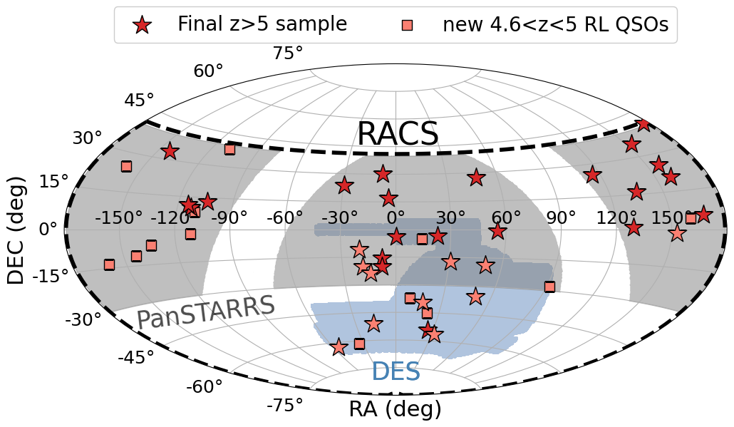
Figure 1: Sky distribution of the final RACS sample together with the area covered by each optical/NIR survey considered and by the RACS-low survey (delimited by the dashed line). The overall area covers $\sim$16000 deg² at $|b|>15^{\circ}$. The stars indicate the $z>5$ sample (darker colour for the quasars already known in the literature and lighter for the new ones reported here), while the squares are the newly discovered sources at $4.5<z<5$.

The manuscript is structured as follows: in Sec. 2 we describe the optical and radio criteria used for the selection of high-$z$ quasars; in Sec. 3 we present the spectroscopic observations and identification of the selected candidates; in Sec. 4 we discuss the completeness of the final $z>5$ sample and compare it to other samples from the literature; in Sec. 5 and 6 we present and discuss the X-ray and radio properties, respectively, of the high-$z$ quasars detected in RACS; finally, in Sec. 7 we summarise our results.

Throughout the paper we assume a flat $\Lambda$CDM cosmology with $H_{0}$=70 km s^-1 Mpc^-1, $\Omega_{m}$=0.3 and $\Omega_{\Lambda}$=0.7. Spectral indices are given assuming S${}_{\nu}\propto\nu^{-\alpha}$ and errors are reported at a 68% confidence level, unless otherwise specified.

2 Selection of high-$z$ radio quasar candidates

In order to build a well-defined sample of $z>5$ radio quasars, we performed a systematic search of these sources in some of the deepest radio and optical/NIR wide-area surveys currently available. In particular, we considered the first data release of the RACS-low survey (low, at 888 MHz; McConnell et al. 2020; Hale et al. 2021) in the radio band together with the DES (2nd data release; Abbott et al. 2021) and the Pan-STARRS (Chambers et al. 2016) in the optical/NIR (both with $grizY$ filters, even though with slightly different bandpasses. The combined footprints of these surveys are shown in Fig. 1.

In this section, we describe the selection of high-$z$ candidates in these surveys mainly through the use of the Ly$\alpha$ dropout technique (e.g., Bañados et al. 2016) together with a radio association (e.g., Caccianiga et al. 2019; Gloudemans et al. 2022).

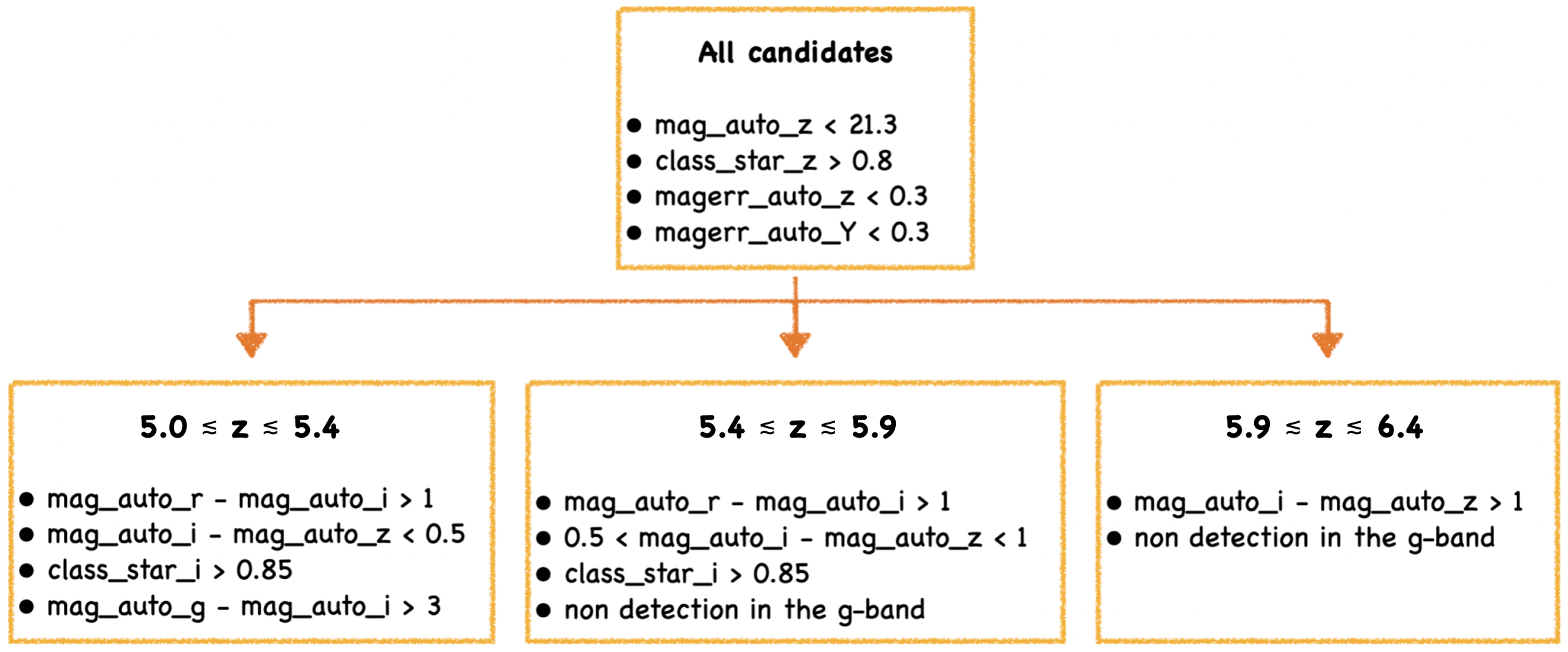
Figure 2: Criteria used for the selection of candidates from the DES survey. The criteria at the top were used for all the candidates, whereas, the criteria at the bottom were used in order to select sources at specific redshifts: (1) for $5\lesssim z\lesssim 5.4$, (2) for $5.4\lesssim z\lesssim 5.9$ and (3) for $5.9\lesssim z\lesssim 6.4$.

2.1 Radio selection in the RACS-low and EMU pilot surveys

We started from the first data release of the RACS-low survey at 888 MHz (McConnell et al. 2020; Hale et al. 2021). We made use of the source lists derived from the images described in McConnell et al. (2020) since the final catalogue of the RACS-low survey built by Hale et al. (2021) has a much larger beam size (25″, a factor $\sim$2 larger than the un-smoothed images) and a comparable RMS (median value $\sim 0.3$ mJy beam^-1 in both cases). This larger beam size would increase the positional uncertainty, especially for faint sources. Given the relatively deep sensitivity of RACS, we were able to select sources with a surface brightness down to $S_{\mathrm{peak}}$ > 1 mJy beam^-1, which would correspond to a S/N $\sim 4$ given the median RMS of the images. In order to reduce the error on the radio position, we only considered objects with an integrated-peak flux density ratio of $S_{\mathrm{int}}$/$S_{\mathrm{peak}}$ < 1.5. This value was chosen to select all the point-like sources in the RACS source lists for S/N as low as $\sim 4$ (see, e.g., section 4.4 in Duchesne et al. 2024). Indeed, as shown also in Sec. 4, most high-$z$ quasars are expected to be point sources. Given the typical positional errors of RACS (about 2^′′ for faint sources, see section 3.4.3 in McConnell et al. 2020), we adopted a flat search radius of 3^′′ to match the radio positions provided in the RACS-low catalogue with the optical counterparts selected as described in the following subsection.

At the same time, we also considered the pilot of the currently on-going EMU survey. While this survey covers a smaller area ($\sim$270 deg²), it has a similar central frequency (944 MHz) and angular resolution ($\sim$18^′′, considering the catalogue from the convolved images, see Norris et al. 2021) compared to RACS-low, with the advantage of being significantly deeper (RMS $\sim 25-30$ µJy beam^-1). Therefore, this catalogue is also instructive on the completeness of the radio selection from RACS. We focused again on sources with $S_{\mathrm{peak}}$ > 1 mJy beam^-1, but since in this case they correspond to a S/N $\gtrsim 30$, we reduced the EMU–DES association radius to 1.5^′′.

2.2 Optical criteria

To select good high-$z$ quasar candidates, we considered the RACS sources that satisfy the criteria outlined above and that are detected in the deepest wide-area optical/NIR surveys currently available: DES and Pan-STARRS.

In both cases, in order to have a flux-limited sample of sources that could be spectroscopically observed in a reasonable amount of time with current ground-based optical telescopes, we restricted the search to sources with a mag$z$ < 21.3. As a reference, the median depth at 5$\sigma$ of the DES and PanSTARRS catalogue considered is 23.6 and 22.1, respectively. We only considered regions of the sky with a Galactic latitude $|b|>15^{\circ}$ to reduce the spurious contamination from Galactic objects. Given the wavelength coverage of the optical/NIR considered surveys, the highest redshift that could be probed is $z\sim 6.8$ (e.g. Bañados et al. 2021), where the Ly$\alpha$ drops-out around the centre of the $Y$ filter. However, in order to have candidates with more secure measurements, we also required a detection in at least two photometric filters. This criterion restricted the search to $z\lesssim 6.4$ sources. Moreover, we note that, since the wavelength coverage of the filters used for the DES and Pan-STARRS surveys are slightly different, also the criteria/threshold adopted in the selection of high-$z$ quasars from each survey is slightly different.

2.2.1 Candidates from the DES survey

To access the most recent data release of DES, the 2^nd (Abbott et al. 2021), we used the dedicated SQL portal. During the selection of new candidates, we considered three different sets of criteria based on the redshift of the potential candidates: (1) for $5\lesssim z\lesssim 5.4$ sources; (2) for $5.4\lesssim z\lesssim 5.9$ sources; (3) for $z\gtrsim 5.9$ sources. The criteria adopted are summarised in Fig. 2, where all the magnitudes are in the AB system.

These criteria are meant to select primarily compact stellar-like objects with a dropout either in the $r$ or in $i$ the filter, hence high values of $r-i$ or $i-z$ colours. Moreover, since we expect the absorption from the IGM to be more effective at shorter wavelengths (i.e., in the $g$-band) and at higher redshift, we also applied a specific magnitude limit in the $g$-band to select only faint objects. In particular, this resulted in a colour mag_auto_g – mag_auto_i $>3$, for sources selected with the criteria (1), expected to be at $5\lesssim z\lesssim 5.4$. This limit selects sources not detected in the $g$-band, or, if detected, with a $g$ magnitude much fainter with respect to the one in the $i$ filter. For candidates at $z\gtrsim 5.4$, instead, we only considered candidates without a detection in the $g$ band. This condition was satisfied by selecting sources with a mag_auto_g $>23.5$ and an error on err_mag_auto_g $>0.5$. Subsequently, we visually inspected the images to discard those with even a faint blue emission. On average, we were able to eliminate all the sources with an emission $\gtrsim 3\sigma$. We note that the $g$-band-faintness criterion was the one that rejected most of the candidates (over 160), especially with the criteria (2), where the Ly$\alpha$ dropout is transitioning from the $r$ to the $i$ band and where stellar contamination is expected to be the predominant (e.g., Yang et al. 2017).

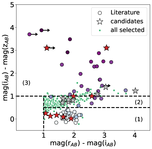
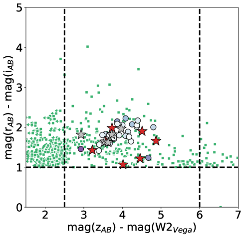
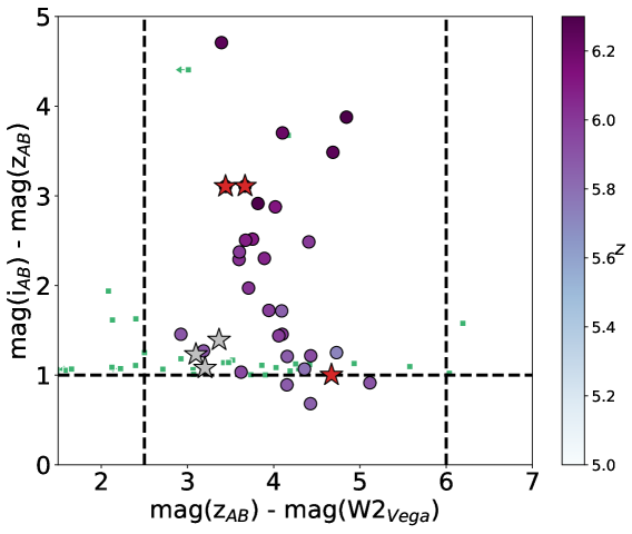
Figure 3: Colour plots used for the selection of candidates from the DES survey. In all the plots the circles represent the already known $z>5$ quasars in the DES area, colour coded based on their redshift. The dashed lines represent the threshold considered in our selection. The small green squares are all the potential candidates selected with the criteria reported in Fig. 2, without the visual inspection of the $g$-band images. Stars indicate the candidates that satisfied all the selection criteria and that form the final well-defined sample: red for confirmed high-$z$ quasars and gray for not-confirmed candidates. Left panel: $i-z$ colour as a function of the $r-i$ one. The plot is divided in three regions, for which different sets of criteria were applied (see Fig. 2), with the aim of selecting sources in specific redshift ranges. As clear from this plot, the region (2) is the one with the most contaminates, likely stars with a spurious radio association. Central panel: $z-W2$ colour as a function of the one around the $r-i$ drop. Right panel: $z-W2$ colour as a function of the one around the $i-z$ drop. The $W2$ magnitude is the only one in the Vega system, the rest are in the AB system. For sources not detected in the $W2$ band, we adopted an upper limit of mag$W2$=19.

After the first selection based on the DES colours, we also considered mid-IR data from catWISE (Eisenhardt et al. 2020; Marocco et al. 2021). For the cross-match, we used a radius of 2.5^′′, which corresponds to $\sim 3\sigma$ the astrometric uncertainty of the faintest catWISE sources (mag_W2 $\sim 17$, Vega system; see fig. 13 in Marocco et al. 2021) and for which we only expect a spurious association chance of $\lesssim 2$%. we only kept candidates with $2.5<\texttt{mag\_auto\_z}-\texttt{mag\_W2}<6$ (where the WISE magnitude is in the Vega system). This criterion is meant to exclude low-$z$ absorbed quasars and part of the elliptical galaxies at low redshift (e.g. Carnall et al. 2015). After applying this filter, we were left with 254 candidates (out of the starting 373). In Fig. 3 we show the $i-z$, $r-i$, and $z-W2$ colours for the $z>5$ quasars currently known in the DES area. At the time of writing, there are a total of 58 $z>5$ quasars with mag$z$ $<21.3$ known in the footprint of DES. We note that not all of these sources have been selected from DES, but also from other surveys with different filter sets (e.g., Wolf et al. 2020; Wenzl et al. 2021; Onken et al. 2022).

2.2.2 Candidates from the Pan-STARRS survey

In order to access the first data release of the Pan-STARRS survey, we used the Mikulski Archive for Space Telescopes (MAST). In particular, we considered the ‘mean’ values reported in the Pan-STARRS catalogue, as opposed to the ‘stacked’ ones. This choice was made in order to have more accurate measurements of the point-like nature of the candidates (see Chambers et al. 2016), since, as detailed below, it is an important constraint in the selection. At the time of writing, the number of $z>5$ quasars in Pan-STARRS ($\sim$350)5 is significantly larger compared to DES ($\sim$60). This is due to many reasons, the main one being that this survey covers a larger fraction of the sky, including the entire northern sky, where more telescopes are available for the spectroscopic follow-up, with respect to the southern sky.

For the Pan-STARRS selection we followed the criteria outlined in Caccianiga et al. (2019) for the selection of a complete sample of radio quasars at $z>4$. Similarly to DES, these criteria are meant to to select point-like objects, faint in the $g$-band, with reliable measurements in the filters red-wards of the expected Ly$\alpha$ and with a drop either in the $r$ or $i$ filter.

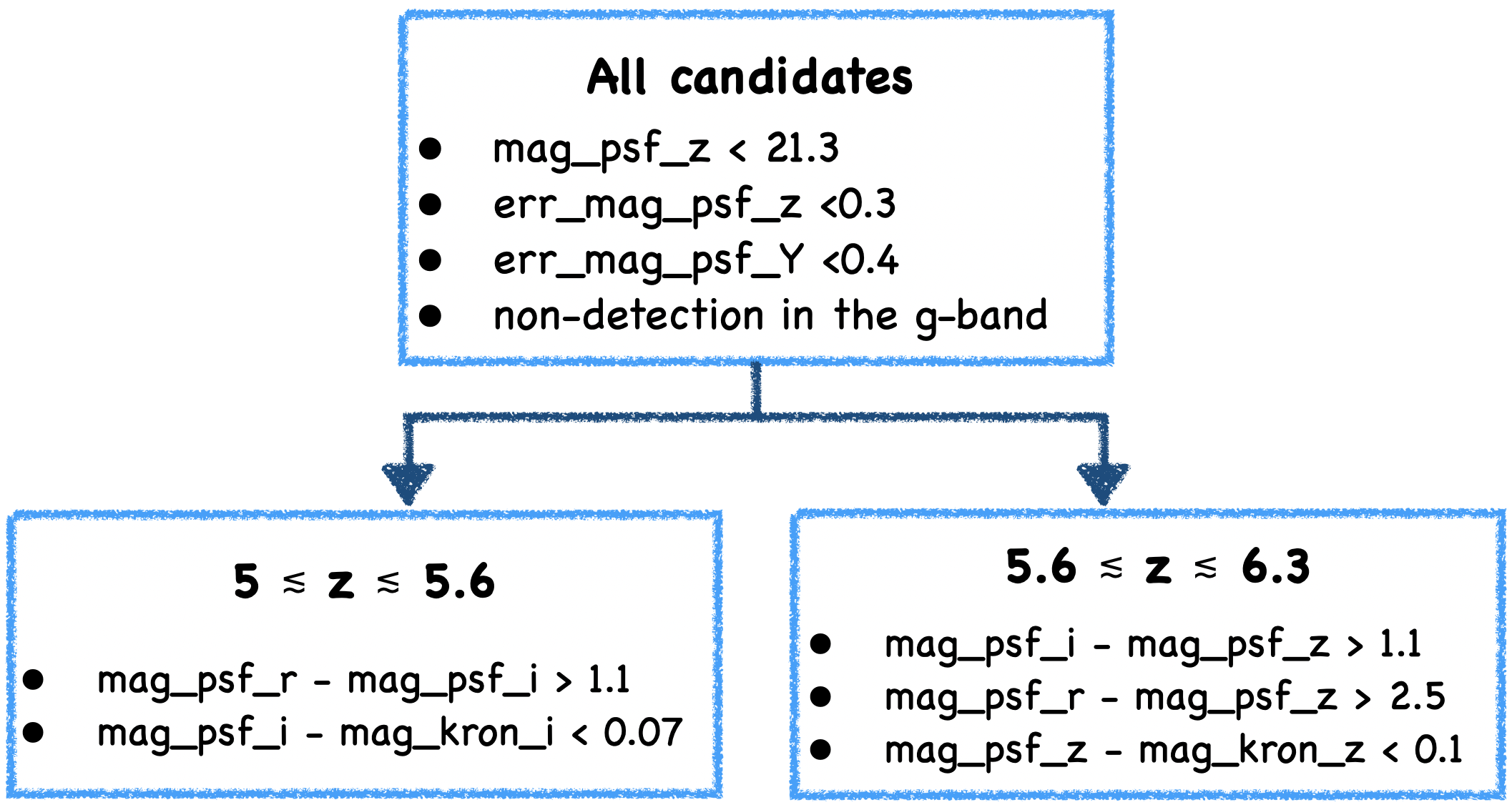
Figure 4: Criteria used for the selection of candidates from the Pan-STARRS survey. The criteria are divided in two sets, one (left) aimed at selecting $5\lesssim z\lesssim 5.6$ candidates and one (right) aimed at selecting $5.6\lesssim z\lesssim 6.3$ candidates. During the selection, we considered the ‘mean’ magnitudes from the PanSTARRS catalogue.

We report the criteria adopted in Fig. 4. As discussed and detailed in Caccianiga et al. (2019), these criteria should recover about $\gtrsim 90$% of the mag_psf_z $<21$ high-$z$ quasars (see also discussion below). Once again the criterion of a non-detection in the $g$-band was initially set to sources with a mag_psf_g $>24$ and then, after applying the IR cut, we checked the $g$-band images of each candidate and discarded the ones where a faint emission was visible (see, e.g., Fig. 15, left panel). In this process we also checked the quality of the other images, since some fields were affected by artifacts. From the visual inspection (performed after the $z-W2$ criterion) we eliminated 27 candidates. After pre-selecting high-$z$ candidates from the Pan-STARRS catalogue with the limits reported in Fig. 4, we also considered the IR magnitudes from the catWISE survey by adopting a matching radius of $2.5^{\prime\prime}$. In this case, to maximise the completeness of the selection we used slightly different limits in the $z-W2$ colour: $z-W2<5$. Indeed, as shown in Fig. 5, in the PanSTARRS selection there are not as many candidates with a non detection in the $W2$, with respect to the DES selection. This is likely due to the slightly different $z$-filters of the two surveys as well as the first $g$-band non detection criterion (i.e. considering a lower limit on the magnitude and its error), which is more efficient in PanSTARRS. After applying this filter 184 candidates were left (out of the starting 439). We show in Fig. 5, the colour distribution of the candidates selected with the criteria just outlined. In the same plot, we also show the colours of the already known $5<z<6.3$ quasars detected in Pan-STARRS.

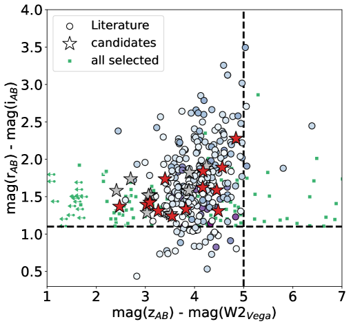
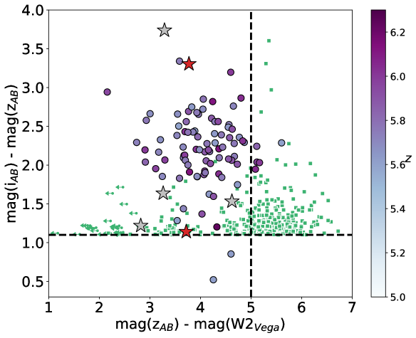
Figure 5: Criteria used for the selection of candidates from the Pan-STARRS survey. The criteria are divided in two sets, one (left panel) aimed at selecting $5\lesssim z\lesssim 5.6$ candidates and one (right panel) aimed at selecting $5.6\lesssim z\lesssim 6.3$ candidates. For clarity, we only show sources at $5<z<5.6$ and at $z>5.6$ in the left and right plot, respectively. For sources not detected in the $r$- or $i$-band we adopted the $5\sigma$ limits of the Pan-STARRS survey for the plot, 23.2 and 23.1, respectively. For sources not detected in the $W2$ band we adopted an upper limit of mag$W2$=19 to plot the data. The dashed lines represent the threshold considered in our selection.

2.2.3 Additional multi-wavelength information

After selecting high-$z$ radio candidates based on the optical/IR magnitudes in the DES, PanSTARRS, and catWISE catalogues, we also used further multi-wavelength information, when available, from other public surveys to discard some contaminants that passed all the selection criteria outlined above.

In particular, we considered the ‘quick-look’ images from the VLA Sky Survey (VLASS; Lacy et al. 2020). The typical RMS of these images is $\sim 120$ µJy beam^-1, which, in principle, is enough to detect at a 3$\times$RMS level even the faintest RACS-low sources we considered, assuming a typical spectral index of $\alpha_{\rm r}\sim 0.7$ (S${}_{\rm 3GHz}\sim 0.43$ mJy beam^-1 for a S${}_{\rm 888MHz}\sim$1 mJy beam^-1 object). Given the better angular resolution ($\sim$4^′′) compared to RACS, this survey also has a better positional accuracy, even though it is limited to Dec. $>-40^{\circ}$. After the visual inspection of the 3 GHz VLASS images, we only kept the candidates where a $>$3$\times$RMS signal, if present, was within 1^′′ from the optical/NIR counterpart. We expect the rest to be spurious associations. In this way we discarded 113 objects.

After the selection based on colour cuts and a reliable radio association in the VLASS survey (if detected), we also considered any available NIR data from the Vista hemisphere Survey (VHS; McMahon et al. 2021) and the VISTA Kilo-degree Infrared Galaxy (VIKING; Edge et al. 2013). For sources with a NIR coverage, we compared their photometric SED to a quasar template and discarded the sources whose NIR and MIR data-points lied systematically above the emission expected from a quasar (see Fig. 15 for such an example). From the template comparison we eliminated 58 candidates in total, most of which are likely low-$z$ elliptical galaxies.

The total number of candidates selected with the optical/IR and radio criteria described above is 45. In particular, one source was selected from the EMU pilot survey (RACS J2020$-$62) and another one (RACS J2142$-$62) was selected in both RACS-low and EMU. We report the selected candidates in Tab. 7 and 4 together with the main optical and radio parameters considered during the selection.

Finally, we note that for one source, RACS J0622$-$51, we obtained a more accurate radio position, with respect to the RACS-low one, based on dedicated observations with the Australia Compact Array (ATCA; see Sec. 6). The new position of the radio source obtained from ATCA is not consistent with the optical counterpart (offset of 3.1″or $>10\sigma$ away; see Fig. 15). For this reason, we classified this source as a non high-$z$ radio quasar.

Table 1: Properties of the 24 candidates confirmed to be at high redshift.

Target	R.A.	Dec.	drop	$z$	$S_{\rm 888MHz}$	mag-$z$	drop	$z-W2$	dro	Telescope
	(deg)	(deg)	(Survey)		(mJy beam-1)	(mag AB)		(AB – Vega)	(arcsec)
RACS J0036$-$37	9.035480	$-$37.095232	$r$-drop (D)	4.95$\pm$0.02	1.3$\pm$0.2	20.49$\pm$0.02	1.66	4.87	1.29	AAT
RACS J0056$-$05	14.245799	$-$5.140481	$r$-drop (D)	4.82$\pm$0.03	1.5$\pm$0.2	21.34$\pm$0.05	1.22	4.46	0.67	VLT
RACS J0110$-$39	17.684618	$-$39.513237	$r$-drop (D)	5.08$\pm$0.03	17.9$\pm$2.1	21.29$\pm$0.05	1.65	3.57	0.89	VLT
RACS J0127$-$44	21.809644	$-$44.912548	$r$-drop (D)	4.96$\pm$0.02	17.9$\pm$2.0	20.67$\pm$0.03	1.42	3.22	1.26	VLT
RACS J0202$-$17	30.618886	$-$17.141042	$r$-drop (P)	5.57$\pm$0.03	17.2$\pm$2.0	19.24$\pm$0.01	1.05	4.17	1.03	AAT
RACS J0209$-$56	32.320529	$-$56.447344	$r$-drop (D)	5.61$\pm$0.03	17.8$\pm$1.8	20.90$\pm$0.02	1.98	3.73	0.39	VLT
RACS J0320$-$35	50.089335	$-$35.351148	$i$-drop (D)	6.13$\pm$0.04	3.2$\pm$0.3	20.59$\pm$0.03	3.11	3.28	1.32	GS
RACS J0322$-$18	50.560622	$-$18.688189	$i$-drop (D)	6.09$\pm$0.04	1.7$\pm$0.2	20.94$\pm$0.03	3.11	3.44	2.59	GS
RACS J0606$-$27	91.605865	$-$27.942459	$r$-drop (P)	4.89$\pm$0.03	13.2$\pm$1.8	20.49$\pm$0.04	1.89	4.56	0.21	AAT
RACS J1011$-$01	152.981424	$-$1.514636	$i$-drop (P)	5.56$\pm$0.03†	8.7$\pm$1.3	21.23$\pm$0.08	1.14	3.72	1.20	GS
RACS J1042+04	160.642581	+4.210405	$r$-drop (P)	4.72$\pm$0.02	1.5$\pm$0.3	21.16$\pm$0.09	1.74	3.40	1.21	LBT
RACS J1321+24	200.260024	+24.896064	$r$-drop (P)	4.78$\pm$0.06	4.6$\pm$1.0	21.04$\pm$0.06	1.31	3.16	0.53	LBT
RACS J1322$-$13	200.526920	$-$13.398532	$r$-drop (P)	4.70$\pm$0.02	37.6$\pm$3.3	20.54$\pm$0.03	1.53	4.68	0.65	NTT
RACS J1426$-$11	216.700593	$-$11.000803	$r$-drop (P)	4.73$\pm$0.05	11.0$\pm$0.7	20.91$\pm$0.05	1.24	3.55	0.56	LBT
RACS J1505$-$06	226.286005	$-$6.708236	$r$-drop (P)	4.53$\pm$0.03	4.8$\pm$1.3	20.74$\pm$0.05	1.31	4.48	0.49	LBT
RACS 1634$-$01	248.603437	$-$1.9576216	$r$-drop (P)	4.88$\pm$0.02	1.8$\pm$0.3	20.25$\pm$0.04	1.37	2.87	0.40	LBT
RACS J1638+08	249.729070	+8.324004	$r$-drop (P)	4.77$\pm$0.02	5.2$\pm$1.5	20.56$\pm$0.04	1.62	4.17	1.26	LBT
RACS J1645+38	251.363676	+38.131409	$r$-drop (P)	4.69$\pm$0.04	2.0$\pm$0.2	21.12$\pm$0.07	1.39	3.02	1.21	LBT
RACS J2020$-$62	305.170194	$-$62.252554	$i$-drop (D)	5.72$\pm$0.02†	1.1$\pm$0.1*	19.23$\pm$0.01	1.00	4.67	0.80	VLT
RACS J2142$-$61	325.615547	$-$61.465918	$r$-drop (D)	4.74$\pm$0.03	4.1$\pm$0.9	19.85$\pm$0.01	1.07	4.02	0.45	VLT
RACS J2240$-$10	340.007219	$-$10.747596	$r$-drop (P)	5.20$\pm$0.03	32.8$\pm$3.4	20.72$\pm$0.04	1.33	3.82	0.65	LBT
RACS J2244$-$20	341.203286	$-$20.130738	$r$-drop (P)	5.41$\pm$0.02	1.5$\pm$0.2	20.64$\pm$0.04	2.28	4.84	0.42	AAT
RACS J2252$-$51	343.029401	$-$51.037899	$r$-drop (D)	5.18$\pm$0.01	9.5$\pm$1.4	19.42$\pm$0.01	1.90	4.51	0.78	AAT
RACS J2303$-$23	345.783262	$-$23.400271	$r$-drop (P)	5.03$\pm$0.03	10.9$\pm$1.5	19.51$\pm$0.02	1.42	3.34	0.54	AAT

3 Spectroscopic identification of the candidates

In order to identify the nature and the redshift of the 45 candidates selected from the cross-match of RACS-low with DES and Pan-STARRS, we performed spectroscopic observations (PI: Ighina) with different ground-based telescopes: Telescopio Nazionale Galileo (TNG; project AOT47_3), Anglo-Australian Telescope (AAT; project O23B005), Gemini-South (GS; projects GS-2021-DD-112 and GS-2023-DD-108), Very Large Telescope (VLT; project 111.24Q5) and Large Binocular Telescope (LBT; projects 2022B_37 and 2023B_22). In one case, RACS J1322$-$13, spectroscopic observations with the ESO Faint Object Spectrograph and Camera (EFOSC2; Buzzoni et al. 1984) at the New Technology Telescope (NTT) were already available, but not published, (project 108.226E.002; PI Decarli).

Almost all of the spectroscopic observations were performed using long-slit spectroscopy. The only exceptions were the observations with the AAT, for which we used the IFU KOALA instrument and, therefore, spectroscopically observed the entire region around the targets.

In order to analyse the observations obtained with different telescopes and instruments, we always followed a standard data reduction detailed in the manual or cookbook of each instrument. During the analysis, we made use of the Image Reduction and Analysis Facility (IRAF; Tody 1986, 1993) software for the reduction of the Gemini–GMOS (with the specific Gemini package), TNG–DOLORES and NTT–EFOSC2 observations, the 2dfdr software (AAO software team 2015) for AAT–KOALA spectra, the SIPGI (Gargiulo et al. 2022) software for LBT–MODS data and the EsoReflex software (Freudling et al. 2013) for the VLT–FORS2 observations. In general, for the reduction of all the observations, we performed the following steps: bias subtraction, flat fielding correction, cosmic rays removal, wavelength calibration and background subtraction. Finally, an absolute flux calibration using the observation of a standard star was applied for sources observed with the LBT and VLT telescopes. In the other cases, we normalised the extracted 1D spectra to the corresponding DES or Pan-STARRS magnitudes.

Out of the 40 candidates spectroscopically observed, 24 turned out to be high-z radio quasars (Fig. 5). While in Fig. 15 we report an example of a candidate not confirmed to be at high redshift. We note that some of the new high-$z$ quasars reported in this study have also been independently identified by other projects during the course of this work: RACS J0056$-$05 (Yang et al. 2023), RACS J0209$-$56 (Wolf et al. 2024), RACS J0322$-$18 (Bañados et al. 2023) and RACS J2020$-$62 (Wolf et al. 2024). Moreover, the spectra of RACS 0202$-$17, RACS J0209$-$56, RACS J0320$-$35, RACS J0322$-$18 and RACS J1011$-$01 were already published in Ighina et al. (2023, 2024a).

In order to estimate the redshift of each source, we considered the composite spectra derived by Bañados et al. (2016) from a sample of $z\gtrsim 5.6$ quasars and performed a fit to the observed optical spectrum of the confirmed candidates. In particular, Bañados et al. (2016) reports three different composite spectra (see their fig. 10), based on the intensity of the Ly$\alpha$ emission line: (i) the median spectrum of the 10% objects with the largest rest-frame equivalent width (Ly$\alpha$+N V); (ii) the median spectrum of all the $\sim 120$ high-$z$ quasars they discovered; (iii) the median spectrum of the 10% with the lowest rest-frame equivalent width (Ly$\alpha$+N V). During the fit we considered all three reference spectra and used the one with the smallest $\chi^{2}_{\rm red}$ to derive the best-fit redshift. The typical uncertainty of this method is about $\sim$0.03, which corresponds to the width of the Ly$\alpha$ drop. For all the sources we obtained satisfactory fit, except in one case, RACS J2020$-$62. The spectrum and the Ly$\alpha$ line of this quasar are strongly affected by intrinsic absorption. For this reason, we estimated the redshift from the OI1303Å  emission line visible at 8754 Å, obtaining $z=5.72\pm 0.02$. Moreover, in the case of RACS J1011$-$01, we considered both the estimate derived from the template fitting as well as the C IV and [C III] emission lines in dedicated NIR observations (see Ighina et al. 2024a).

As clear from Fig. 6, while our selection targeted $z>5$ quasars, the majority of the newly discovered sources is at $4.5<z<5$. This is mainly due to the large variety of shapes in the rest-frame UV emission of quasars (e.g. in terms of Ly$\alpha$ strength), which results in sources at different redshift ($\Delta z\sim 0.3$) having similar photometric colours and dropout. For example, RACS J1505$-$06 at $z=4.53$ and RACS J2240$-$10 at $z=5.20$ have a similar dropout in PanSTARRS ($r-i\sim 1.3$) despite being at very different redshift. The large number of $z<5$ sources in our final sample indicates that the fixed cuts adopted in their photometric selection were conservative enough to recover the majority of the $z>5$ quasars, even the ones with small dropouts. As described below, we only focus on the $z>5$ objects when it comes to building a complete sample for future statistical works, since we expect the completeness of our selection to quickly decreases at $z\lesssim 4.9-5$. Nevertheless, in this paper we also present their X-ray and radio properties since they are not discussed in other works.

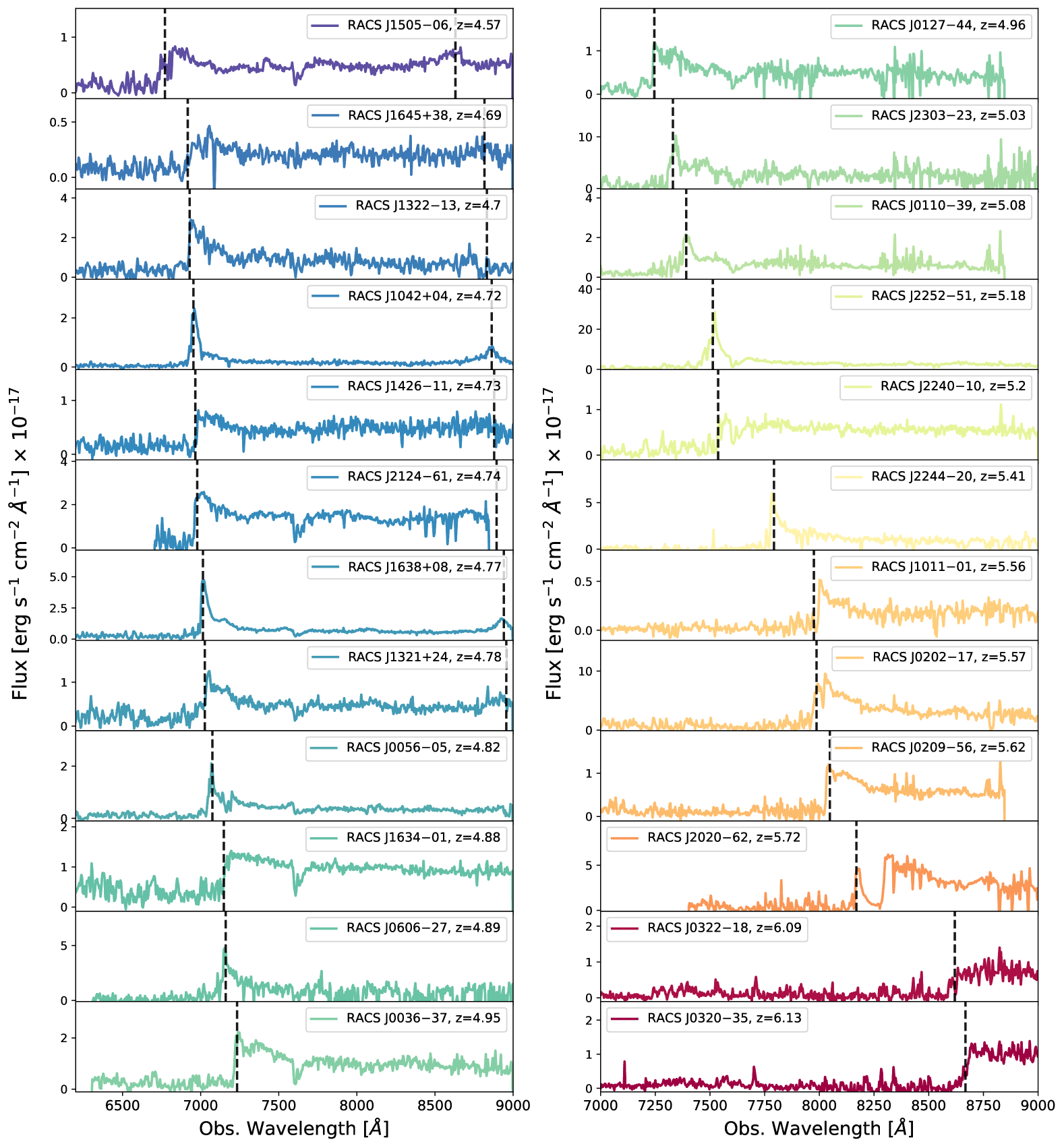
Figure 6: Optical spectra centred on the Ly$\alpha$ emission line and dropout of the newly discovered $4.53\leq z\leq 6.13$ radio quasars from the RACS sample. The sources are ordered in increasing redshift and the dashed vertical line in each plot indicates the expected wavelength emission of the Ly$\alpha$1215 (and CIV1549) in the observed frame. The absorption feature observed at $\sim$7600 Å  in several spectra is due to the O II in our atmosphere.

Although, in principle, the radio association should have prevented stars from being selected as potential candidates (albeit some rare cases of radio emitting stars exist; e.g., Gloudemans et al. 2023a), many of the sources not confirmed to be at high redshift were actually stars. Indeed, at least 9 out of the 17 contaminants in our selection, turned out to be stars (mainly brown dwarfs, see, e.g., Fig. 7, left). The remaining sources are either low-$z$ radio galaxies, or their exact nature could not be determined, apart from excluding the high-$z$ nature due to the lack of a sharp drop in the flux. Therefore, in most of these cases the radio-optical association must be spurious, that is, with the stars falling within 3″of a RACS radio source by chance, although some stars have been found to be radio emitters (e.g. Gloudemans et al. 2023a; Driessen et al. 2024). As expected, most of these sources are faint in the radio band (S${}_{\rm 888MHz}<2$ mJy) or at Dec. $<-40^{\circ}$ and could not be detected or observed as part of the VLASS survey. An example of spurious radio association is the object RACS J0622$-$51, which, when observed with higher resolution radio observations, has an optical position not consistent with the associated RACS-low source (see Sec. 6 and appendix A). On the other hand, a particularly interesting example of a candidate identified as a brown dwarf with a RACS-low flux of $\sim 13$ mJy beam^-1 less than 0.4^′′ from the optical counterpart is RACS J1521$-$21 (see spectrum in Fig. 15).

If we compare the radio-to-optical distance of all the selected candidates (see Fig. 7, left panel), it is clear how the majority (15 out of 24) of the confirmed high-$z$ sources have a radio association within 1^′′ from their optical position. Whereas, only 3 sources out 17 that have not been confirmed to be at high redshift have a radio signal in the RACS-low survey at a distance $<1^{\prime\prime}$.

At the same time, we can also estimate the likelihood of finding a non-radio, high-$z$ quasar close, by chance, to an unrelated radio source in RACS. To this end, we considered the bright end ($M_{\rm 1450}<-27.3$; corresponding to mag$z$ $<$ 21.3 at $z\sim 5$) luminosity function of $z\sim$5 quasars derived by Niida et al. (2020) and estimated the expected number of bright quasars per square degree in the redshift range $z=5-6$, resulting in $\sim$0.01 deg^-2. Multiplying this number for the area used in our search, $\pi r^{2}=\pi(3^{\prime\prime})^{2}\sim 2\times 10^{-6}$ deg², we obtain the probability that a random position is within 3^′′ of a $z\gtrsim 5$ quasar: $\sim 3\times 10^{-8}$. If we consider also the number of radio sources used for the association ($\sim 1.3\times 10^{6}$ in 16000 deg²; e.g. McConnell et al. 2020), the probability of selecting one $z\gtrsim 5$ quasar based on a spurious radio association in RACS is about 4%. Since the majority of the confirmed quasars have an association within $1.5^{\prime\prime}$ (for which we would expect $\sim 1$% of spurious associations) and, more importantly, the association is supported by additional radio data, it is unlikely that any of the quasars discovered is not responsible for the observed radio emission.

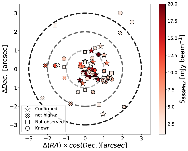
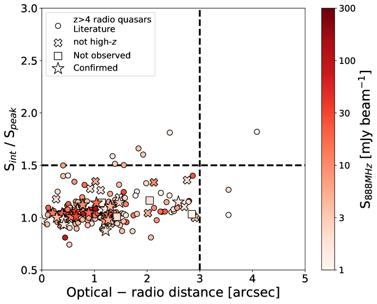
Figure 7: Left panel: Offset in declination as a function of the offset in right ascension between the optical positions from DES or Pan-STARRS and the radio positions from RACS-low for the high-$z$ candidates as well as the already known $z>5$ radio quasars with the same flux limits. The colour of the data points reflects the peak flux density of the given source in the RACS-low source lists as shown by the colour-bar. The dashed circles represent a separation of 1, 2 and 3^′′. Right panel: Distribution of the integrated-to-peak flux density ratios from RACS-low as a function of the optical-to-RACS position for the $z>4$ radio quasars currently known in the RACS area. The colour of the markers indicates the peak flux density reported in the RACS-low source lists. The dashed black line are the threshold used during our selection.

4 RACS sample of high-$z$ radio quasars

In this section we discuss the sample selected from the RACS radio survey. In particular, we estimated the completeness of our selection for $z>5$ sources, which is given by the combination of the optical and the radio selection processes. We also compared the distribution of the RACS sources comapred to other high-$z$ samples of radio quasars from the literature.

4.1 Completeness of the selection

With the optical/NIR criteria reported above, we recovered about 96% of the $z>5$ quasars (not necessarily radio) already known in the DES area and about 85% of those $z>5$ in the Pan-STARRS area. The two sources not recovered in the DES selection were not selected due to their class_star_z parameter being $<0.8$. Whereas, in the case of Pan-STARRS quasars, the majority (51 objects, $\sim$15%) of the quasars were not selected due to dropout (mag_psf_r -- mag_psf_i $>1.1$ or mag_psf_i -- mag_psf_z $>1.1$) and/or the point-like criteria (mag_psf_i -- mag_kron_i $<0.07$ or mag_psf_z -- mag_kron_z $<0.1$).

Since the sources discovered in the literature cannot be considered a complete sample, as demonstrated in the previous section, the fraction of $z>5$ quasars recovered is not a good estimate to the actual completeness of our sample. In order to have a more accurate estimate of the optical completeness of our selection we considered the region of the sky given by $09<{\rm RA}<16$ and $0^{\circ}<{\rm Dec.}<60^{\circ}$, which is fully covered by the Sloan Digital Sky Survey (SDSS; Abdurro’uf et al. 2022) and for which the level of completeness of $z<5.5$ bright (mag$z$ $<21$) quasar is close to 100%. Indeed, there have been several studies aimed at uncovering all the $z>5$ quasars present in this region in order also to constrain the luminosity function of these objects (see, e.g., Fan et al. 1999a, b, 2000; Jiang et al. 2008; Wang et al. 2016; Niida et al. 2020). Moreover, as expected, no new $z>5$ radio quasars were discovered in this same area in our selection, apart from two $z\sim 4.7$ quasars with mag$z$ $>21$. For these reasons, we considered all the bright (mag$z$ $<21$) quasars at $5<z<5.5$ available in the footprint of the SDSS between 09h$\leavevmode\nobreak\ <{\rm RA}<\leavevmode\nobreak\$16h, a total of 82 objects, and checked their colours in the Pan-STARRS survey, since there is no overlap with the DES survey. After applying the criteria reported in Fig. 4 as well as the $W2$ selection, we recover 68 sources, corresponding to the 83% of the initial sample. We consider this value as bona-fide estimate of the optical completeness in the RACS sample, also for the selection of sources at $z>5.5$ and for sources selected in DES, for which a complete reference sample is not available yet. But we stress that, technically speaking, this is an upper limit on the optical/NIR completeness of the overall sample.

A first discussion on the completeness of the radio selection using the RACS source lists was already presented in Ighina et al. (2023) and here we report a brief summary. To assess the completeness of the RACS-low survey when it comes to point-like and relatively faint radio sources, we considered the ASKAP observations of the 23^rd GAlaxy Mass Assembly (G23; Driver et al. 2011) field described in Gürkan et al. (2022). This field covers 83 deg² in the southern hemisphere (centred at RA = 23h and Dec = $-$32^o) at the same frequencies of first scan of RACS-low (888 MHz) and with a similar angular resolution ($\sim$10^′′), but with a sensitivity about an order of magnitude deeper (RMS$\sim$38 µJy beam^-1). In order to estimate the detection completeness of the RACS-low survey, we checked how many sources with S_int/S${}_{\mathrm{peak}}<1.5$ and with $1<$ S${}_{\mathrm{peak}}<100$ mJy beam^-1 (i.e., similar to the targets we selected) in the G23 ASKAP observation are reported in the source lists of RACS-low used in this work as a function of radio flux density. From this comparison, we found that the overall radio selection is about 78% complete for S${}_{\mathrm{888MHz}}>1$ mJy beam^-1 increasing to 93% for S${}_{\mathrm{888MHz}}>2$ mJy beam^-1.

Finally, in order to estimate the fraction of sources missed from the radio-optical association of 3^′′ and the requirement of compact radio sources (S_int/S${}_{\mathrm{peak}}<1.5$), we considered all the currently known quasars at $z>4$ detected by the RACS-low survey (164 in total; to the best of our knowledge). The fraction missed due to either of these criteria is $\sim$6% ( 10 objects), see Fig. 7 for the distribution of the optical–radio distances and of the integrated/peak flux ratio. There are three sources that have been missed by both criteria and the majority of sources not included has a surface brightness $<3$ mJy beam^-1 This suggests that the fractions of sources not selected with the different radio criteria are not independent and a larger incompleteness is expected for faint sources. For this reason, we assume that the completeness of our radio selection criteria is 75% for $>1$ mJy beam^-1 (90% for $>2$ mJy beam^-1). If the selections were completely independent to each other, these values would be only slightly smaller, by $\sim$2% and, therefore, would not significantly change the results presented throughout this work.

4.2 The final RACS sample

As mentioned before, we only consider $z>5$ quasars as part of the final RACS sample, for which we expect the completeness of the selection to be relatively high. By considering similar $z>5$ quasars with S${}_{\mathrm{888MHz}}>1$ mJy beam^-1 and mag$z$ $<21.3$, and by applying the optical and radio selection criteria listed in the previous section, we recover 12 out of the 22 radio quasars currently reported in the literature. We list in Table LABEL:tab:list_known the radio quasars already discovered in the same area and at the same optical and radio flux density limits as our selection. If an already known source is not selected by our criteria, we also indicate the reason. In order to confirm whether a known $z>5$ quasar with mag$z$ $<21.3$ was detected in RACS or not, we checked the images centred on the optical position of all such sources reported in the literature, assuring a detection of faint sources slightly above the 3$\sigma$ (i.e., not reported in the source lists).

In particular, six high-$z$ radio quasars are not selected because of their radio association. As expected, all of them have a flux density between 1 and 3 mJy. Two of these quasars were not selected due to their large optical-to-radio offset ($\sim$3.5^′′), three because the RMS of the image was too high to select a $S_{\rm 888MHz}\sim 1-3$ mJy object and the last one was not selected due to its S_int/S_peak, being $\sim 1.6$.

At the same time, four already known $z>5$ radio quasars were not selected from the Pan-STARRS survey due to their optical properties. One of the sources, RACS J1427+33 at $z=6.12$, was not selected because it is not reported in the Pan-STARRS catalogue, probably due to the presence of a contaminating nearby bright object (at $\sim 3^{\prime\prime}$). Indeed, McGreer et al. (2006) discovered this quasar thanks to the FLAMINGOS Extragalactic Survey (FLAMEX; Elston et al. 2006), which covers a 4.1 deg² region in the $J$ and $K_{s}$ filters. For this object we report in Table LABEL:tab:list_known the magnitude in the $z$ filter computed based on the one in the filter $J$ and assuming a slope of the spectrum $\alpha_{\nu}^{\rm o}=0.44$ (e.g. Vanden Berk et al. 2001). One target was not recovered since it is not detected in the $Y$-filter of Pan-STARRS (i.e., err_mag_Y $>0.4$) and two high-$z$ quasars were not selected due to the point-like requirement, either in the $i$ or $z$ filter.

The overall completeness of the selection criteria adopted here, obtained from combining the radio and optical completeness derived from reference samples, is 0.83 $\times$ 0.75 =0.62, which increases to 0.75% for $S_{\rm 888MHz}>2$ mJy beam^-1. Based on the 22 $z>5$ sources (newly discovered and from the literature) recovered from our criteria, we would expect a total of 22/0.62 $\sim 35-36$ radio quasars with the same optical and radio flux limits in the area we considered. Including the eleven radio quasars already reported in the literature that were not recovered by our selection, we still expect to be missing $\sim$3-4 objects, resulting in a final completeness of the RACS $z>5$ sample of $\sim 90$%. We also note that, while there are still 4 objects without spectroscopic identification, only a fraction is expected to be at high redshift. Indeed, by assuming the efficiency of this work in selecting $z>5$ radio quasars ($\sim$25%) the expected number of true $z>5$ is $\sim 1$. Since this corresponds to $\sim 3\%$ of the final RACS sample, well within the Poisson errors, we do not include them in the following discussion.

Combining all the already known $z>5$ radio quasars from the literature (22) with the new $z>5$ ones identified in this work (11), the final sample built from the combination of RACS, DES and Pan-STARRS is composed by 33 objects that span a redshift range $5<z<6.13$. In Fig. 1 we report the sky distribution of all the high-redshift sources detected in RACS sample. The $z>5$ radio quasars in the sample are distributed evenly in the Pan-STARRS (27 in 12850 deg²) and DES (10 in 5000 deg²) areas, with four sources covered by both, suggesting that the two selections have a similar completeness.

4.3 Comparison with other high-$z$ radio samples

Being a radio and optically selected sample, it is valuable to compare its redshift and luminosity distribution to other samples of high-$z$ radio quasars.

In Fig. 8 we report the monochromatic radio and optical luminosity distribution of the sample (left panel) as well as the redshift and radio-loudness parameter distributions (right panel). This last parameter is defined as $\rm R\leavevmode\nobreak\ =S_{\rm 5GHz}/S_{4400\AA }$ in the rest frame (Kellermann et al. 1989) and quantifies the strength of the radio emission compared to the optical/thermal one. In the same plots, we also show the distributions of other samples of high-$z$ radio quasars from the literature: the CLASS sample (Caccianiga et al. 2019), the FIRST sample (Caccianiga et al. 2024) and the radio quasars detected in LoTSS (Gloudemans et al. 2021, 2022). The CLASS sample was built from the combination of Pan-STARRS together with the Cosmic Lens All Sky Survey (Myers et al. 2003), which includes sources with $S_{\rm 5GHz}>30$ mJy and $\alpha_{1.4}^{5}<0.5$. In particular, a dedicated search for $z>4$ radio quasars led to an almost complete ($\sim 95$%) sample of 24 sources with mag $<$21 (in the filter longwards the Ly$\alpha$ drop, which depends on the redshift) over an area of $\sim$13100 deg^-2 at $|b|>20^{\circ}$. Given the high radio flux limit and the criterion on the radio spectral index, the CLASS sample contains mostly blazars, as demonstrated by the X-ray analysis of the full sample (Ighina et al. 2019). The FIRST sample, instead, was built considering the $z>4$ quasars in the SDSS ($09<{\rm RA}<16$ and $0^{\circ}<{\rm Dec.}<60^{\circ}$), which, as mentioned before, should be complete for sources with mag $<$ 21, detected in the Faint Images of the Radio Sky at Twenty-Centimetres (FIRST; Becker et al. 1995) radio survey. The radio flux limit of this sample is 0.5 mJy beam^-1 at 1.4 GHz (i.e., $3\leavevmode\nobreak\ \times$ RMS of the survey) and is composed by 73 radio quasars that cover an area of $\sim$5215 deg². The final comparison sample corresponds to all the $z>5$ quasars from the literature detected in the 2^nd data release of the LoTSS survey (38; Gloudemans et al. 2021) as well as 24 newly discovered $z\gtrsim 4.9$ radio quasars selected from the combination of LoTSS and the DESI Legacy Imaging Surveys (Dey et al. 2019). We note that while the RACS, CLASS and FIRST sample are built with both a radio and optical flux limit, the sources detected in LoTSS do not have a defined optical threshold, even though most of them were discovered in similar optical/NIR surveys as the other samples.

To compute the optical and radio luminosities for the different samples, we proceeded as described below. For the sources detected in LoTSS, we used the measurements and the method reported in Gloudemans et al. (2021, 2022). In particular, we considered $\alpha_{\rm r}=0.3$ for the radio spectral index (with uncertainty $\sigma_{\alpha}=0.2$) if not reported. For the three remaining samples, we considered the optical/IR magnitudes in the $z$ and $W1$ filters in order to estimate the spectral index of the optical spectrum. Then, using each spectral index and the $W1$ magnitude, we computed the 4400 Å  rest-frame luminosity, while from the $z$ magnitude we computed the 2500Å  luminosity. We chose these two filters since all the sources have been detected in both of them, and they are the closest to the 2500 and 4400 Å  rest-frame wavelength, respectively. To compute the radio luminosities at 5 GHz (rest frame) of the CLASS and FIRST sources, we considered the flux density at 1.4 GHz, from either the FIRST or NVSS survey, and the spectral index computed between 1.4 GHz and 150 MHz (from either the TGSS or LoTSS survey). We can expect variability to potentially affect the value of the spectral index observed, especially for the most radio-luminous sources. However, Caccianiga et al. (2019) estimated the amplitude of variation for the CLASS sample to be $\sim$14% at 1.4 GHz in the observed frame, hence not enough to significantly change the values reported here. For sources without a 150 MHz detection (about half of the sample), we considered the median spectral index of the detected quasars, $\alpha_{0.15}^{1.4}\sim 0.1$ (with uncertainty $\sigma_{\alpha}=0.2$). We note that only by assuming a significantly different value for $\alpha_{0.15}^{1.4}$ the overall distribution of the sample changes. Indeed, by assuming $\alpha_{0.15}^{1.4}\sim 0.3$, the mean variation in luminosity of the sample corresponds to $\sim$5%. In the case of the RACS sample, we used the spectral indices derived from the fit of the low-frequency radio spectrum (see Sec. 6). The errors reported only include the uncertainty on the flux densities and do not include those associated with the spectral indices. If a source belongs to the RACS sample as well as another sample, only the marker corresponding to the RACS sample is reported in Fig. 8. However, the histograms include all the sources in the given sample. In Table LABEL:tab:lum_RACS_sample we report the monochromatic luminosity and the radio-loudness parameter of the high-$z$ quasars detected in RACS.

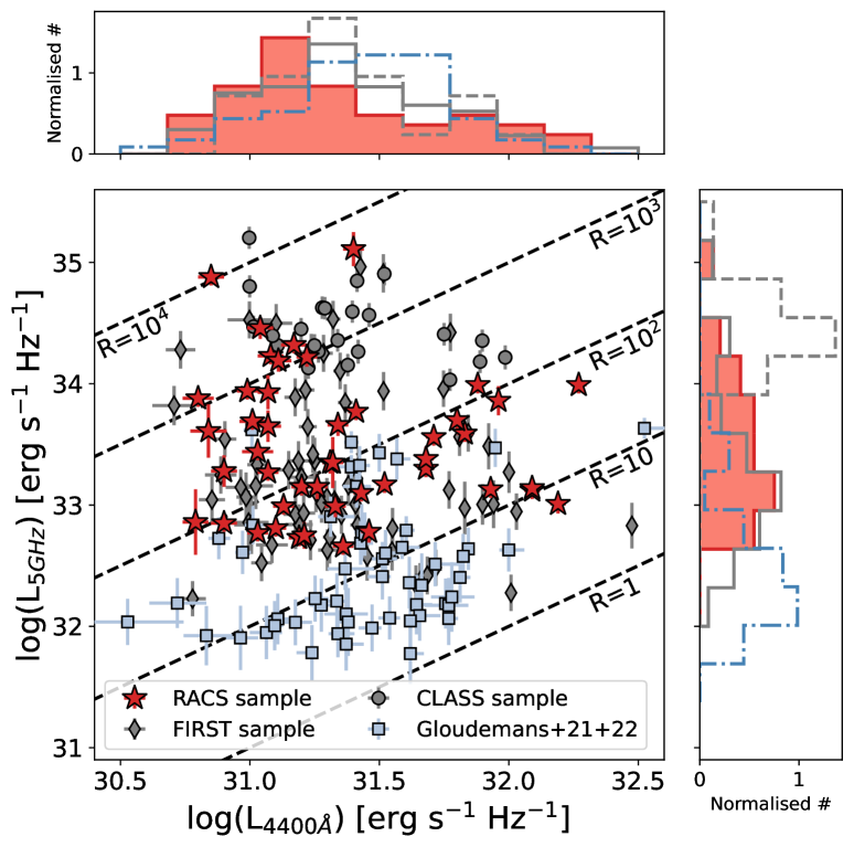
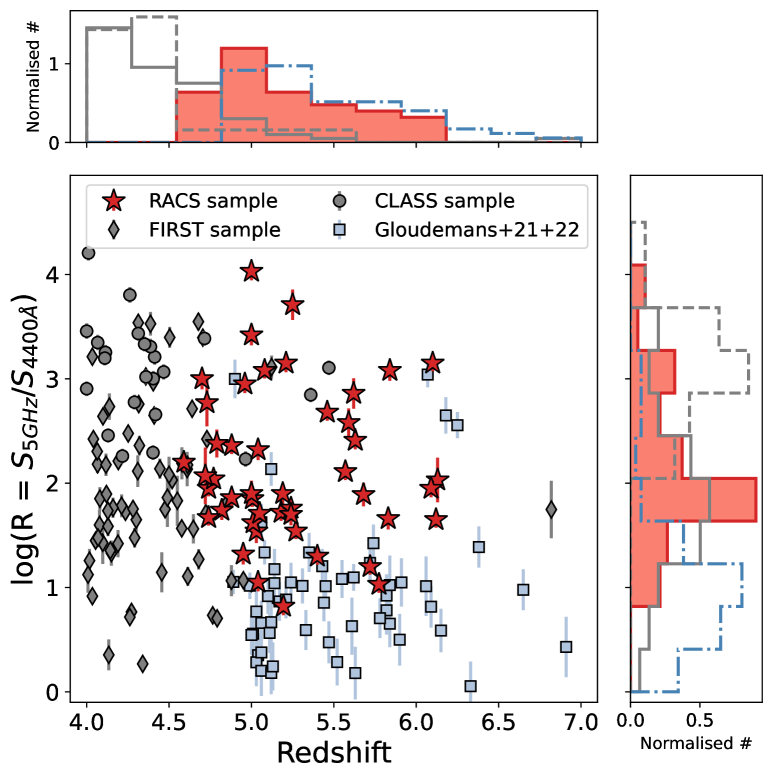
Figure 8: Left panel: Radio (5 GHz) and optical (4400 Å) monochromatic luminosity distributions of the high-$z$ sample selected with RACS. The sample includes the new high-$z$ quasars discovered during this project as well as the $z>5$ radio quasar already reported in the literature. The newly discovered quasars at $z<5$ are reported in light blue, whereas the remaining $z>5$ RACS quasars are reported in dark blue. Grey diamonds and circles indicate the FIRST sample described in Caccianiga et al. (2024) and the CLASS sample described in Caccianiga et al. (2019), respectively. The light-blue squares are the high-$z$ radio quasars detected in LoTSS (from Gloudemans et al. 2021, 2022). Right panel: radio loudness, R $=S_{\rm 5GHz}/S_{4400\AA }$, and redshift distribution of the RACS sample, together with the FIRST and CLASS ones. The symbols are the same as in the left panel. The histograms in both panels show the distribution of the given parameter for each sample (CLASS = dashed, FIRST = solid empty, LoTSS = dashed-dotted and RACS = filled histogram).

From Fig. 8, it is clear that all the samples cover a very similar range of optical luminosities. This is expected since they have been built using a similar optical limit and/or surveys. At the same time, different samples cover different values in radio luminosities: while the CLASS sample is mainly composed by very bright objects, the sources detected in LoTSS are mainly concentrated on the low end of the radio luminosity distribution. Again, this is also due to the radio flux limits (and frequencies) used in the selection of the different sources. Indeed, while the CLASS sample has a limit $\sim$30 times larger compared to the RACS and FIRST samples, the LoTSS survey has an RMS$\sim$90 µJy beam^-1. By taking a deeper look, the median radio luminosity of the RACS sample (logL_5GHz $\sim$ 33.4 erg sec^-1 Hz^-1) is slightly larger compared to that of the FIRST one (logL_5GHz $\sim$ 33.1 erg sec^-1 Hz^-1), even though well within the dispersion of their distributions. This is likely due to the different redshift distributions of the two samples, with the RACS sample probing higher redshift and, therefore, higher luminosities for a similar radio flux limit. A similar effect can also be seen in the distribution of the optical luminosities, where the relative number of high-luminosity quasars in slightly larger in the RACS sample. Indeed, as shown in the right panel, while the majority of the FIRST sample are in the redshift range $4<z<5$, most of the RACS sources, by construction, are at $5<z<6$. At the same time, the LoTSS survey, thanks to its depth, is able to uncover many objects at $z>6$, even though many of them are relatively radio faint (L${}_{\rm 5GHz}<10^{33}$ erg sec^-1 or R $\lesssim 10$).

Based on the plots in Fig. 8, it is clear that the RACS sample contains the brightest radio quasars currently known at $z>5$. For this reason, this is the ideal starting point to identify blazars, that is, quasars with a relativistic jet oriented close to our line of sight (e.g. Padovani & Giommi 1995), and to constrain the properties and evolution of the jetted quasar population at $z>5$ (see e.g. Diana et al. 2022; Caccianiga et al. 2024; Bañados et al. 2025). In the following three sections we present the data/observations currently available for this sample in the X-ray and radio bands

5 X-ray observations and detections

While the number of radio quasars has significantly increased in the last few years (e.g. Gloudemans et al. 2022; Belladitta et al. 2023; Bañados et al. 2025), only a small fraction of these sources have been observed at high energies, namely in the X-rays (e.g. Medvedev et al. 2020, 2021; Khorunzhev et al. 2021; Moretti et al. 2021; Connor et al. 2021). In this section we report and discuss the X-ray detections of the sources within the RACS sample in the first data release of the German eROSITA All-Sky Survey (eRASS:1; Merloni et al. 2024. We also present the analysis of dedicated Chandra-X-ray observations on a newly discovered $z>6$ quasar (RACS J0322$-$18).

5.1 Information from eRASS and literature

The eRASS:1 survey covers a total of 22 quasars from the RACS sample discussed in this work. Among them, three of the newly identify objects are detected in the soft 0.2–2.3 keV band and reported in the eRASS:1 catalogue. We present in Table 2 their main X-ray properties from catalogue. X-ray luminosities were computed assuming a photon index value of $\Gamma_{\rm X}=2.0$ (see, e.g., Vignali et al. 2005; Nanni et al. 2017). In particular, RACS J2020$-$62 and RACS J0127$-$44 (at redshift $z=5.72$ and $z=4.96$, respectively) are the most distant objects currently identified in this catalogue. The high-redshift nature of these sources, together with the detection in the eRASS:1 scan, make these objects extremely X-ray luminous. However, the RACS J2020$-$62 quasar is not detected in later eRASS scans and dedicated Chandra observations revealed an X-ray emission more than one order of magnitude fainter (see Wolf et al. 2024), suggesting that the X-ray flux reported in the Merloni et al. (2024) catalogue might have been caused by a variable or transient event.

For RACS J0127$-$44 and RACS J1322$-$13, the large observed X-ray luminosities indicate that the high-energy emission in these systems is dominated by relativistic effects (e.g., Ghisellini 2015), classifying these systems as blazars. Indeed, the corresponding $\tilde{\alpha}_{\rm ox}$ parameters, defined as $\tilde{\alpha}_{\rm ox}=0.303\times{\rm log(L_{10keV}/L_{2500{A}})}$ (Ighina et al. 2019), are consistent with the ones derived for the blazar population ($\lesssim 1.36$; e.g., Ighina et al. 2024a). Furthermore, also the radio emission of both these systems is flat ($\alpha_{\rm r}<0.5$; see Sec. 6) and strong with respect to the optical one (R$\sim$1000), hence strengthening their blazar classification (e.g. Caccianiga et al. 2019).

Dedicated X-ray observations are also available for the majority of the $z>5$ sources already discussed in the literature. We report in Table LABEL:tab:lum_RACS_sample the $\tilde{\alpha}_{\rm ox}$ parameter for all the objects with X-ray information together with the corresponding references for the X-ray emission. For sources covered in eRASS:1, but not detected, we report a lower limit on their $\tilde{\alpha}_{\rm ox}$ parameter based on the $3\sigma$ upper-limit provided by the eRASS:DE consortium at any given position in the sky and assuming again $\Gamma_{\rm X}=2.0$, as in Merloni et al. (2024). We note that all the $\tilde{\alpha}_{\rm ox}$ values estimated from dedicated X-ray observations are consistent with the lower limits derived from the eRASS:1, when available.

We show in Fig. 9 the $\tilde{\alpha}_{\rm ox}$ parameter as a function of redshift for the RACS sources with X-ray coverage. In the same plot, we also show the median value obtained for $z\sim 4.5$ blazars from Ighina et al. (2019) ($\tilde{\alpha}_{\rm ox}=1.1$) as well as the expected values for radio-quite quasars with a similar optical luminosity, log(L_2500Å / erg sec^-1 Hz^-1) = 30.7–32.0, based on the UV-X-ray relation derived by Lusso & Risaliti (2016) (assuming $\Gamma_{\rm X}=1.7-2.1$). While the $\tilde{\alpha}_{\rm ox}$ values in the RACS sample are not as extreme as the radio-brighter blazars at $z=4-5.5$ from the CLASS sample, they have, on average, a stronger X-ray emission (i.e., lower $\tilde{\alpha}_{\rm ox}$ values) compared to what we would expect from thermal emission only, as in the case of radio-quiet quasars. This suggests that blazars compose a large fraction of the RACS sample, for which the high-energy emission is dominated by the relativistically boosted emission produced by the jets.

Table 2: X-ray properties from the eRASS:1DE catalogue (Merloni et al. 2024) of the newly discovered sources in this work.

Name	$z$	Flux[0.2-2.3keV]	Lum[2-10keV]	net counts	distance	Det. likelihood
RACS J0127$-$44	4.96	4.2${}^{+2.0}_{-1.6}$	7.1${}^{+3.5}_{-2.9}$	6.7	10.2	8.9
RACS J1322$-$13	4.70	12.6${}^{+3.4}_{-2.8}$	18.7${}^{+6.7}_{-4.7}$	19.2	4.4	44.8
RACS J2020$-$62	5.72	6.7${}^{+3.2}_{-2.4}$	15.7${}^{+7.1}_{-5.6}$	7.4	17.7	10.0

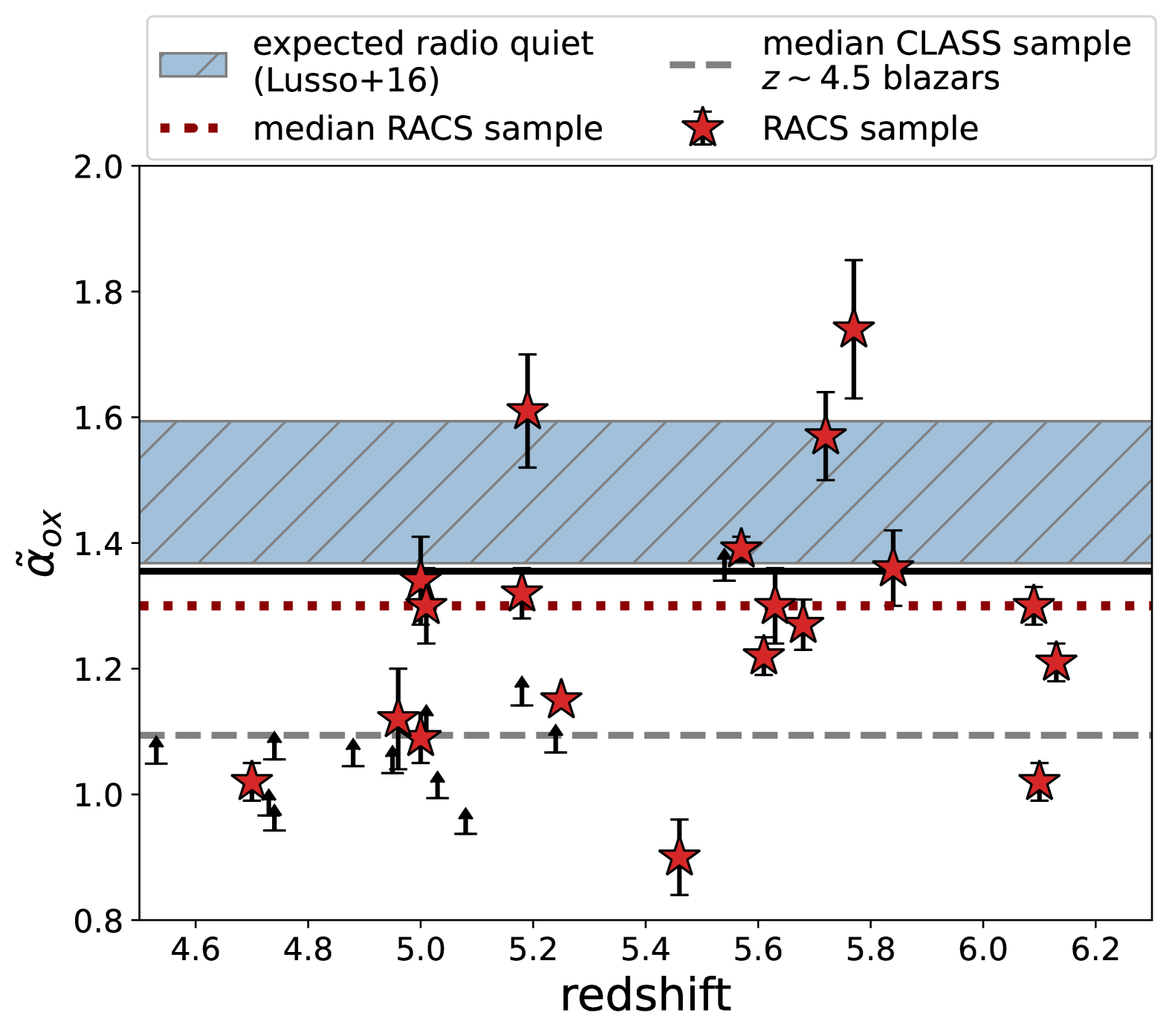
Figure 9: $\tilde{\alpha}_{\rm ox}$ of the RACS sources with X-ray coverage as a function of their redshift. The dotted red line shows the median value of the RACS sources with an X-ray detection, while the dashed gray line is the median value of the blazar sample analysed in Ighina et al. (2019). The dashed blue area showed range of values expected from the X-ray corona (i.e., from a radio-quiet quasar) with a monochromatic UV luminosity similar to the RACS sample, logL${}_{2500\AA }=30.7-32.0$ erg sec^-1 Hz^-1, based on the relation described in Lusso & Risaliti (2016) and assuming a photon index in the range $\Gamma=1.7-2.1$.

5.2 Chandra observations

We obtained dedicated Chandra observations for two of the most-distant quasars discovered in our selection, RACS J0320$-$35 and RACS J0322$-$18 (Proposal 24700061; PI: Ighina). In this section we discuss and analyse the observation of RACS J0322$-$18, while the high-energy properties of RACS J0320$-$35 are presented in a separate, dedicated paper (Ighina et al. in preparation).

RACS J0322$-$18 was observed for a total of 90 ksec, with 30 ksec observed in 2024 February and 60 ksec observed in 2024 June, for a total of six exposure segments. Observations were performed using the Advanced CCD Imaging Spectrometer (ACIS; Garmire et al. 2003) in the Very Faint telemetry format and Timed Exposure mode and with the target positioned on the back-illuminated S3 chip. The observations analysed in this work are contained in the Chandra Data Collection (CDC) CDC 323. We reduced the observations using CIAO (v. 4.16; Fruscione et al. 2006) with CALDB (v4.11.2). We show in Fig. 10, top panel, the 0.5–7.0 keV image obtained from the combination of the different exposures. We used specextract to extract events from a 2″  source region and from a background annulus of 10–$30^{\prime\prime}$, both centred on the optical/NIR position of the quasar. An X-ray source is detected, with 52 net counts over a background of $\lesssim$1, at the optical position of the quasar. We then analysed the extracted spectra using XSPEC v 12.11.1 (Arnaud 1996) and performed a fit minimizing the modified C-statistic (Cash 1979; Wachter et al. 1979). We binned the 0.5–7.0 keV spectrum to one net count per energy bin and we modelled it with a simple power law absorbed by the Galactic column density along the line of sight (wabs$\times$pow), fixed to N${}_{\rm H}=3.04\times 10^{20}$ cm^-2 (HI4PI Collaboration et al. 2016). We report in Table 3 the parameters derived from the best fit. In Fig. 10, bottom panel, we show the X-ray photon spectrum convolved with the instrumental response. We note that the discrepancy between the data and the simple power law model at energies $<1$ keV is not significant and more complex models are not statistically favoured.

Interestingly, while the best-fit photon index value has a relatively large uncertainty, $\Gamma_{\rm X}=2.1\pm 0.5$, the small value of the $\tilde{\alpha}_{\rm ox}$ parameter, $\tilde{\alpha}_{\rm ox}=1.30\pm 0.03$, is consistent with what is normally found in blazars (e.g., Ighina et al. 2019; Sbarrato et al. 2022). This would make RACS J0322$-$18 one of the highest-redshift blazars currently known, with only other two identified at $z>6$ (see Belladitta et al. 2020; Bañados et al. 2025). Very long baseline interferometric (VLBI) observations are needed to strengthen this classification (e.g., Coppejans et al. 2016).

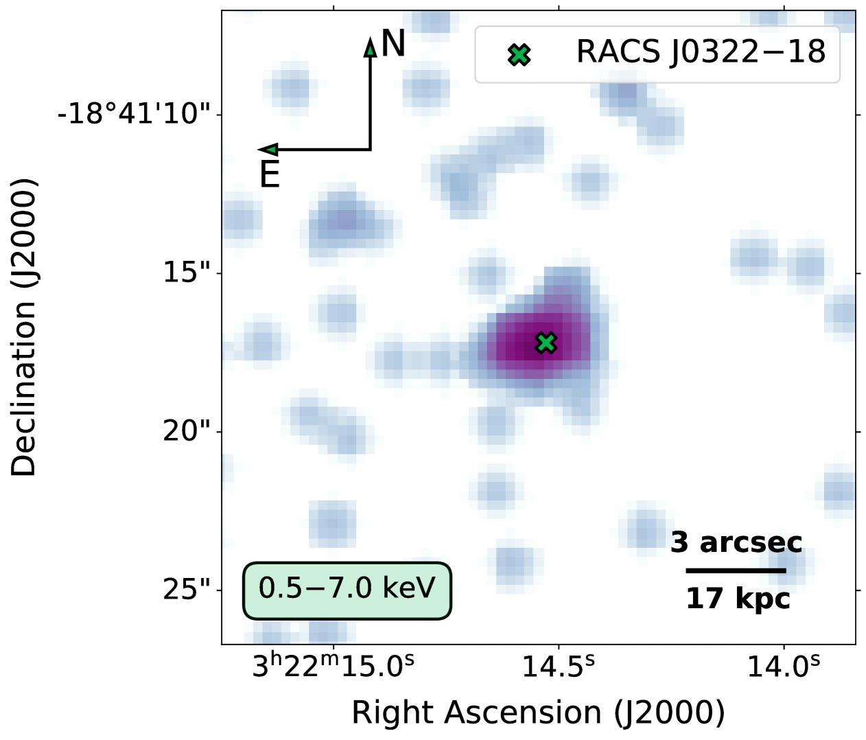
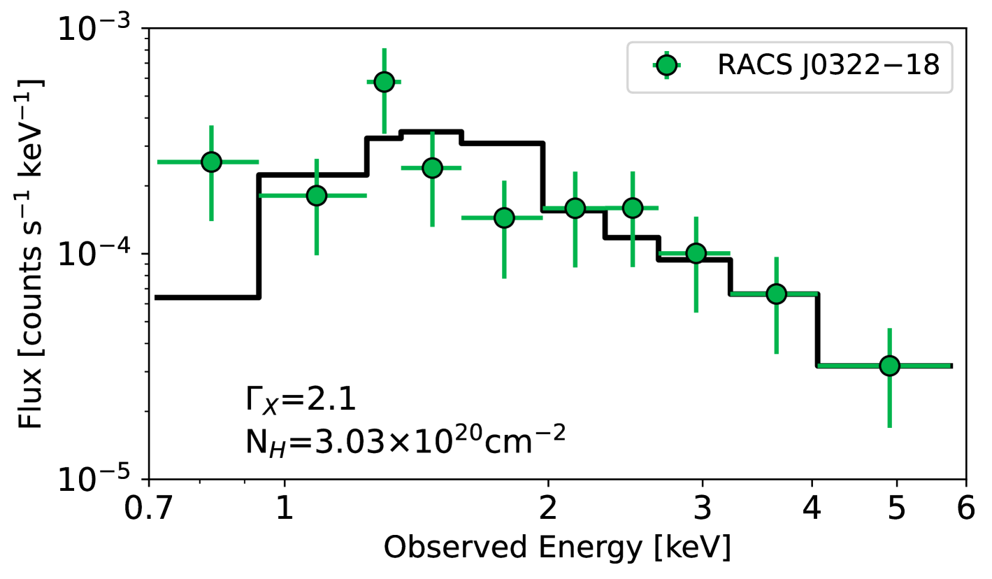
Figure 10: Top panel: 0.5–7.0 keV image of RACS J0322$-$18. The green cross indicates the optical/NIR position of the quasar. Bottom panel: Best-fit model, including a power-law with Galactic absorption (solid black line), over-plotted on the X-ray Chandra spectrum of RACS J0322$-$18.

Table 3: Results from the analysis of the X-ray spectrum of RACS J0322$-$18.

$\Gamma_{\rm X}$	Flux[0.5-7keV]	Lum[2-10keV]	cstat/d.o.f.
2.1$\pm 0.5$	1.07${}_{-0.04}^{+0.13}$	3.1${}_{-1.3}^{+2.5}$	35 / 51

6 Radio properties

In this section we describe the radio properties of the high-$z$ quasars discussed in this work. The analysis is based on measurements available from public surveys, as well as dedicated radio observations performed on a sub-set of the sample. We report the data analysis of dedicated radio observations in appendix B.

6.1 Surveys and dedicated observations.

Thanks to the large variety of radio surveys performed in the last few years, many data-points covering frequencies in the observed range 70 MHz–3GHz are available for a given high-$z$ radio-bright quasar (depending on its sky position and intensity). In particular, we considered the measurements available from the following surveys: the Galactic and Extra-Galactic All-Sky MWA survey (GLEAM); Wayth et al. 2015, 2018; Hurley-Walker et al. 2017, the specific survey covering the south Galactic pol (GLEAM-SGP; Franzen et al. 2021) and the extended survey (GLEAM-X; Hurley-Walker et al. 2022; Ross et al. 2024), at frequencies between 70 and 230 MHz; the LoTSS (Shimwell et al. 2017, 2019, 2022), including the deep fields (Tasse et al. 2021; Sabater et al. 2021), at 144 MHz; the TIFR GMRT Sky Survey (TGSS; Intema et al. 2017) at 150 MHz; the Westerbork In the Southern Hemisphere (WISH; De Breuck et al. 2002) survey at 352 MHz; the Sydney University Molonglo Sky Survey (SUMSS; Mauch et al. 2003) at 843 MHz; the RACS-low survey (McConnell et al. 2020; Hale et al. 2021); the continuum measurements from the MeerKAT Absorption Line Survey (MALS; Deka et al. 2024) at 1 GHz; the first scan of the RACS-mid survey (Duchesne et al. 2023, 2024) at 1.37 GHz; the FIRST (Becker et al. 1995) survey at 1.4 GHz, the NRAO VLA Sky Survey (NVSS; Condon et al. 1998) at 1.4 GHz; the quick-look images from the VLA Sky Survey (VLASS; Lacy et al. 2020; Gordon et al. 2020) at 3GHz.

For all the targets, we first considered the radio detections as reported in each official catalogue. If no detections were reported, we checked the images and considered as detections all those sources with a signal $>3\times$ the off-source RMS otherwise we considered this value as upper limit. For sources detected in VLASS, we applied a 15% (to the 1.1 epoch) or 8% correction (to the other epochs) to increase the peak flux densities derived from the images and considered an additional 10% of the flux density when computing the corresponding uncertainty, added in quadrature

Moreover, we included the flux density measurements as reported in the source lists of the ASKAP telescope observations taken as part of the following projects: the 3^rd data release of RACS-low at 944 MHz, the 1^st data release of RACS-high at 1.67 GHz (Duchesne et al. 2025) and the Evolutionary Map of the Universe (EMU; Norris et al. 2021) at 944 MHz. Since these estimates are not part of a final catalogue, we added in quadrature a further 10% to their uncertainties. All of the radio quasars discussed here are compact on $\sim 10$″scales, based on their the VLASS radio images, which is expected for these high-$z$ sources (e.g. Capetti & Balmaverde 2024). The only exception is RACS J0309+27, discussed in Ighina et al. (2022b) which shows an extended component consisting of only $\sim$4% of the core flux. For these reasons, we do not expect the different angular resolution to play a significant role in the radio flux density recovered in each survey.

Finally, we also considered dedicated radio observations discussed in the literature as well as data newly obtained as part of this project (with the upgraded Giant Metrewave Radio Telescope, uGMRT, MeerKAT and ATCA). We provide the details of these observations in appendix B.

6.2 Radio spectra

We present in Fig. 11, 12 the radio spectra of the RACS–selected $z>5$ quasars based on the data-sets described in the previous sub-section. Moreover, we show the radio spectra of the newly discovered $4.5<z<5$ radio quasars in appendix C. Thanks to the low-frequency coverage of the GLEAM-X, TGSS and LoTSS surveys as well as the high-frequency coverage of the VLASS survey and the dedicated ATCA observations, we are able to constrain the radio emission of most systems over a very large range of frequencies. Although some radio sources may present a very complex spectral shape with multiple components (see, e.g., Shao et al. 2022; Ighina et al. 2022a), in this work we limit the analysis of the radio spectra to simple power laws. In particular, for each object we performed a fit to all the data-points available with a simple power law:

$$S_{\nu}=N\times\nu^{-\alpha}$$ (1)

and a broken power law:

$$S_{\nu}=\begin{cases}N\times(\nu/\nu_{\rm break})^{-\alpha_{\rm low}}&\text{if $\nu\leq\nu_{\rm break}$}\\ N\times(\nu/\nu_{\rm break})^{-\alpha_{\rm high}}&\text{if $\nu>\nu_{\rm break}$}\\ \end{cases}$$ (2)

To perform the fit we used the MrMOOSE code (Drouart & Falkendal 2018a, b), which also takes the upper-limits into account. This is especially important for sources with a non-detection at low frequencies, for which the limited frequency coverage of the detections would result in a highly uncertain estimate. During the fit, we added a further 10% to the flux density measurements in order to account for the typical radio variability of quasars (e.g. Barvainis et al. 2005; Tinti et al. 2005; Liu et al. 2009). We do note that strong variability ($>$10%; as expected in some blazars; Sotnikova et al. 2024) can significantly affect the observed shape of the emission, for example introducing a peak in the spectrum (Mingaliev et al. 2012).

In order to choose the model that better reproduces the observed data-points, we compared their relative likelihood with the Akaike Information Criteria (AICc; Akaike 1974; Burnham 2002) defined as:

$${\rm AICc}=2k-2{\rm ln}(L)-\frac{2k(k+1)}{n-k-1}$$ (3)

where $n$ the number of data points, $k$ the number of free parameters (two in eq. 1 and four in eq. 2), and ln($L$) the maximum of the likelihood function (calculated with MrMoose). The lower the value of the AICc parameter is, the better the model describes the observations. We note that the $2k$ term in eq. 3 penalises the addition of free parameters and the last term is a further correction in case of a limited number of data points. We report the best-fit spectral index and break frequency values obtained from the fit in Tab. LABEL:tab:lum_RACS_sample and we show the best-fit models in Fig. 11 and 12 (Tab. 18 and Fig. 16 for sources at $z<5$).

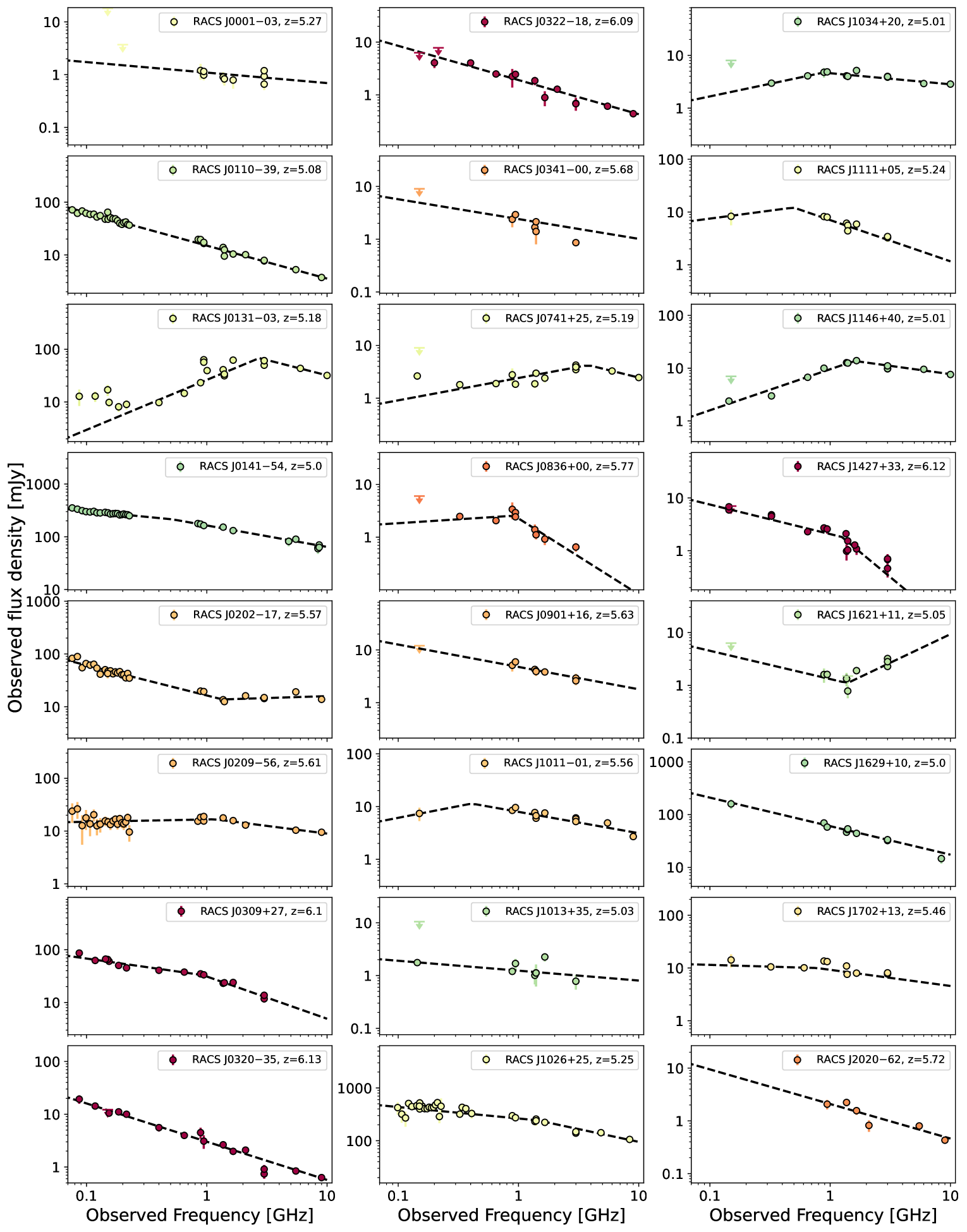
Figure 11: Radio spectra of the newly discovered sources in the RACS sample in order of increasing redshift (colour-coded with the same scale of Fig. 6). Radio data-points are mainly from publicly available surveys, as described in the text, as well as from dedicated ATCA, uGMRT and MeerKAT observations on a subset of objects. The dashed black line show the best-fit power law (or broken power law) function.

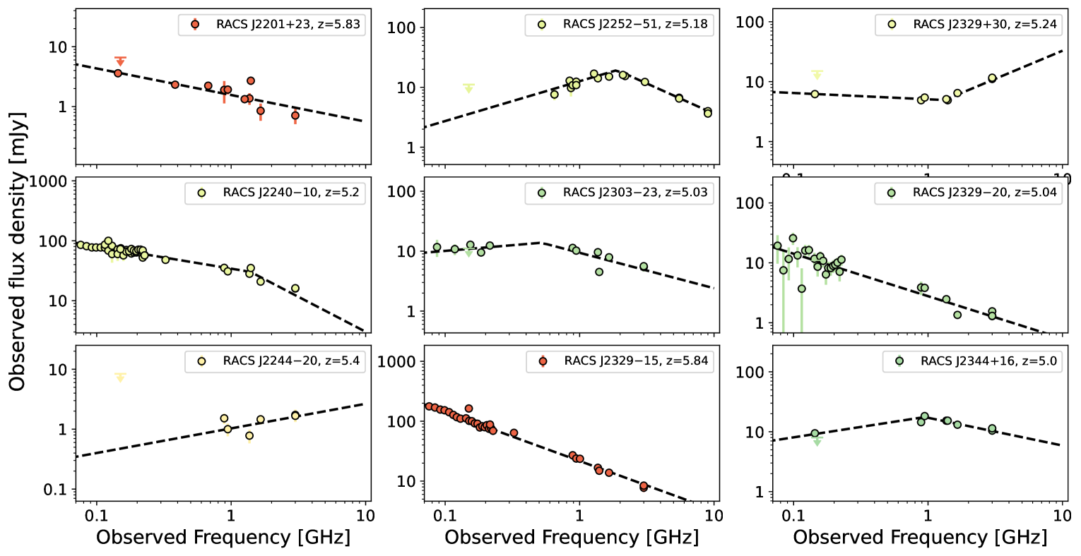
Figure 12: Continuation of Fig. 11

Despite the simple models assumed, a power law effectively describes the radio emission in a given frequency range for the majority of the sources. In total, a simple power law model was favoured for half of the sample (23 out of 46 objects; 15 out of 33 at $z>5$). As expected, most of these objects have a limited frequency coverage (namely lack of detections at $<800$ MHz or $>2$ GHz).

In Fig. 13 we show the best-fit distribution of the radio spectral indices and break frequencies derived with MrMOOSE. The majority of the RACS sample presents a spectral index, both at low and high frequencies, in the range $\sim 0.0-0.8$. On average, the high-frequency emission is steeper (median value $=$0.45) than the one at low frequency (median value $=$0.32). We note that, by considering the $z>5$ quasars only, the distributions and the median values change only slightly (0.48 and 0.22, for ${\alpha}_{\rm high}$ and ${\alpha}_{\rm low}$, respectively) . These values are on the lower end of the distribution of radio spectral indices found at lower redshift. For example, Calistro Rivera et al. (2017), considering $z<2.5$ AGN selected from the SDSS mean value $\bar{\alpha}=0.7$ with a dispersion of $\sigma=0.3$ in the 0.1–1.4 GHz observed range. This is likely due to a selection effect; with the RACS-low survey we are only sensitive to relatively luminous high-$z$ quasars (L${}_{\rm 5GHz}\gtrsim 10^{33}$ erg s^-1 Hz^-1) at a rest-frame frequency of $\sim$5 GHz and, therefore, we expect a significant fraction of the radio emission to be relativistically boosted. Similar values were found when considering the $z>4$ quasars detected in FIRST (0.1 and 0.4 at low and high frequencies, respectively; Caccianiga et al. 2024) as well as very radio-luminous (L${}_{\rm 5GHz}\gtrsim 10^{34}$ erg s^-1 Hz^-1) $3<z<4$ quasars (0.0 and 0.4 at low and high frequencies, respectively; Sotnikova et al. 2021).

Based on a Gaussian fit of the spectral index distributions we find that low-frequency spectral indices have a mean value $\bar{\alpha}_{\rm low}=0.20$ and a standard deviation $\sigma_{\rm low}=0.45$, while high-frequency spectral indices have $\bar{\alpha}_{\rm high}=0.44$ and $\sigma_{\rm high}=0.52$.

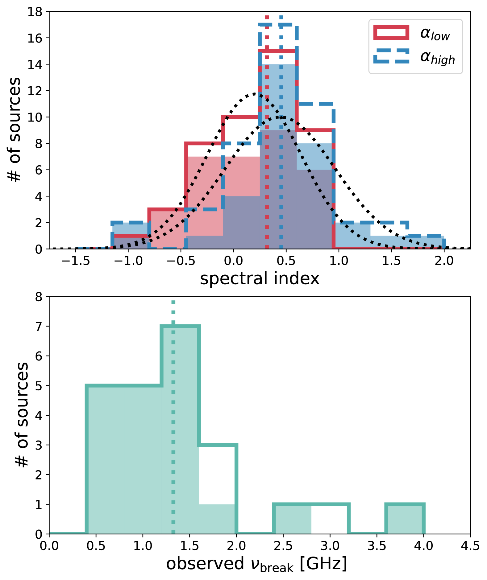
Figure 13: Top panel: Distribution of the $\alpha_{\rm low}$ and $\alpha_{\rm high}$ parameters derived for all the radio quasars discussed in this work. In case of a single power law fit, the spectral index is considered in both distributions. Dotted vertical lines indicate the median values of each spectral index distribution (0.32 and 0.45 for $\alpha_{\rm low}$ and $\alpha_{\rm high}$, respectively). The best-fit Gaussian distributions are shown with dotted black lines. Bottom panel: Distribution of the break frequency in the observed frame for all the sources were a double power law was favoured. Dotted vertical line is the median value (1.3 GHz). In both panels, the distribution of $z>5$ sources is highlighted with filled histograms.

If we compare the values derived for the spectral indices at low and high frequencies for each source (Fig. 14) the quasars in the RACS sample occupy different regions of the plane, which can be interpreted as different physical properties. A large fraction of the sample lies within the region delimited by a spectral index $=\pm 0.5$ (23 in total, 15 of which at $z>5$). This is the threshold commonly used in the literature to identify flat-spectrum radio quasars (i.e. blazars; e.g. Sotnikova et al. 2021), for which we expect the radiation to be dominated by strong Doppler boosting due to jet being oriented close to our line of sight. Indeed, two of the newly discovered quasars detected in the eRASS:1 (see Sec. 5) are in this region. Identifying blazars in a well-defined sample, as the one discussed here, is extremely important to constrain the evolution of the entire jetted population, especially at high redshift (see, e.g., Diana et al. 2022; Sbarrato et al. 2022). However, further observations (especially X-rays and VLBI) are needed to accurately constrain the nature of these systems, since variability might affect the observed shape of their radio spectra.

A small fraction of the RACS quasars shows typical $\alpha_{\rm low}\sim 0.5$ values with a significant steepening at higher frequencies, $\Delta\alpha\gtrsim 0.4$. This type of steeping at high frequencies has already been observed in other high-$z$ radio sources (see, e.g., Drouart et al. 2020; Spingola et al. 2020) and is typically associated with the radiative cooling of the most energetic electrons in the extended regions of the jets (e.g. Harwood et al. 2013; Morabito et al. 2016).

There are also significant outliers from the one-to-one relation, having opposite spectral indices at low and high frequencies (top left and bottom right regions in Fig. 14). In particular, sources with $\alpha_{\rm low}<0$ and $\alpha_{\rm high}>0$ present a peak in their radio spectrum, typically around $\sim 1$ GHz in the observed frame (see HZQ J1146+40 and RACS J2252$-$51), which corresponds to frequencies $>6$ GHz in the rest frame. These ‘peaked spectrum’ radio sources are normally associated with young and compact relativistic jets that are still expanding in the surrounding medium (e.g., Dallacasa et al. 2000; Orienti & Dallacasa 2012, 2014; O’Dea & Saikia 2021). In particular, we note that in the case of RACS J2252$-$51 the presence of a peak at $\sim 2$ GHz in the observed frame is confirmed by simultaneous MeerKAT observations covering the 1–3 GHz frequency range. Dedicated low-frequency and VLBI observations on this high-$z$ system are crucial to constrain the origin of this turnover and therefore to constrain intrinsic properties of the jet (e.g., magnetic field) or the external environment (e.g., electron density; Gloudemans et al. 2023b) via spectral modelling and morphology studies (e.g.; Keim et al. 2019; Shao et al. 2022).

On the other side of the plot, objects with $\alpha_{\rm low}>0$ and $\alpha_{\rm high}<0$ present a so-called ‘up-turn’. The radio spectrum of these objects is probably composed of the radiation produced by different jet components. For example, it can be caused by a steep emission of an extended, not resolved component and a flat/inverted emission of the core (see e.g. Behiri et al. 2025)or also by the presence of a double peak in the radio spectrum (see, e.g., fig. 2 in Shao et al. 2022).

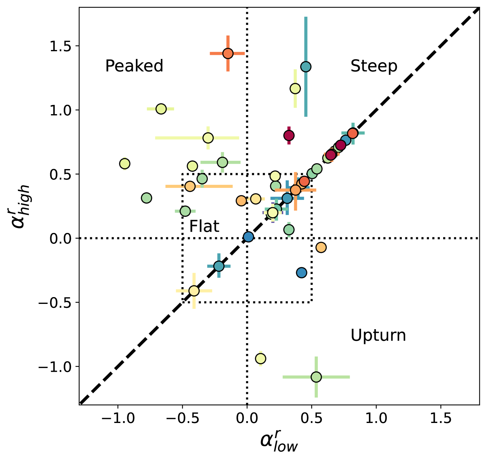
Figure 14: Low-frequency ($\alpha_{\rm low}$) and high-frequency ($\alpha_{\rm high}$) radio spectral indices of the radio quasars discussed in this work. For clarity reasons, we only show values with an uncertainty on both spectral indices $\sigma<0.7$. Sources with a single power law fit are shown on the 1:1 relation (dashed black line). Objects with a single power law fit are reported in this line. The dotted lines at $\alpha=0,\pm 0.5$ divide the space in different regions, as discussed in the text.

7 Summary and conclusions

We summarise here the main results reported in this work.

• Sample selection: from the combination of the RACS-low, DES, and Pan-STARRS surveys, we selected a sample of 45 high-$z$ radio quasar candidates, well-defined in radio, optical, and NIR flux limits and colours, with S${}_{\rm 888MHz}>1$ mJy and mag$z$ $<21.3$ over an area of 16000 deg² (see Sec. 2). Based on the number of $5<z<5.5$ quasars selected in the deeply explored SDSS area, we estimate our optical/NIR completeness to be $\sim$83%. At the same time, based on the comparison of the RACS-low survey with similar, deeper ASKAP observations and based on the selection of already known $z>4$ radio quasars, we estimate the completeness of our radio selection to be $\sim 75\%$ for surface brightness S${}_{\rm 888MHz}>1$ mJy beam^-1 and $\sim 90\%$ for S${}_{\rm 888MHz}>2$ mJy beam^-1. The overall completeness of our selection is therefore $\sim 62\%$ at S${}_{\rm 888MHz}>1$ mJy beam^-1 and $\sim 75\%$ at S${}_{\rm 888MHz}>2$ mJy beam^-1 (see Sec. 4).
  

• Identification and final sample: we obtained spectroscopic observations for the majority of the selected candidates (40 out of 44) with the AAT, Gemini-South, LBT, NTT, TNG and VLT. We confirmed the high-$z$ quasar nature of 24 of the candidates, including 11 at $z>5$ (see Fig. 6). Considering the quasars already known from the literature that are also recovered from our selection criteria, we built a sample of 22 radio quasars at $z>5$ with S${}_{\rm 888MHz}>1$ mJy and mag$z$ $<21.3$. Given the estimated level of completeness (62% above 1 mJy beam^-1), we expect that in the surveyed sky area and at the radio/optical limits of our sample, there are $\sim$35 $z>5$ quasars, $\sim$13 of which were missed by our selection. However, we recovered many (11) of these missing sources from the literature, thus obtaining a final sample of 33 $z>5$ radio quasars which we expect to be $\sim$90% complete (see Table LABEL:tab:lum_RACS_sample).
  

• X-ray band: detections or strong upper-limits—are available for $\sim$55% of the $z>5$ quasars (18 out of 33, or 20 out of 46 including sources at $z<5$). This information mainly comes from dedicated X-ray observations available from the literature (e.g. Moretti et al. 2021; Connor et al. 2021; Zuo et al. 2024) or obtained as part of this project (e.g., Ighina et al. 2024a). In particular, from dedicated Chandra observations of RACS J0322$-$18 at $z=6.09$ (see Fig. 10) revealed a relatively bright X-ray emission, compared to the optical/UV one ($\tilde{\alpha}_{\rm ox}=1.30\pm 0.03$), making this one of the highest redshift blazars currently known. At the same time, four sources in the RACS sample have also been detected as part of the eRASS:1 survey (e.g. Khorunzhev et al. 2021; Wolf et al. 2024), three of which were discovered as part of this work, including one at $z>5$ (RACS J2020$-$62; independently discovered by Wolf et al. 2024). These sources represent the highest-redshift quasars currently detected in this first scan. In general, the X-ray emission of the selected sources is systematically larger compared to that expected from radio-quiet quasars, having an $\tilde{\alpha}_{\rm ox}$ parameter larger than the one expected for radio-quite quasars (based on the Lusso & Risaliti 2016 relation). The strong X-ray emission observed in our sources is likely associated with the radiation produced by the relativistic jets, indicating that many of the radio-bright quasars we selected are blazars.
  

• Radio band: combining measurements and upper-limits from wide-area radio surveys (e.g., GLEAM-X, LoTSS, TGSS, NVSS, RACS, VLASS) together with newly obtained dedicated observations (with uGMRT, MeerKAT and ATCA), we were able to constrain the radio shape of the high-$z$ quasars detected in RACS-low over a very wide range of frequencies, $\sim 0.1-10$ GHz (observed frame; see Fig. 11, 12 and 16). We do note that simultaneous radio observations are available for only a small fraction of the entire sample and variability can still play a significant role in these measurements. From the fit of the radio data-points below and above 1.4 GHz in the observed frame, we found that most of the sources have a radio slope in the range $0.0-0.7$, with a median spectral index of 0.31 and 0.46 at low and high frequencies, respectively (see Fig. 13). However, some notable outliers are also present, showing clear signs of a peak or of an upturn in the radio spectrum. At the same time, a third of the $z>5$ radio quasars (12 out of 33) presents a flat radio spectrum (i.e. $-0.5<\alpha_{\rm r}<0.5$ at both low and high frequencies; 22 including $z<5$ sources). Once again, the large number of quasars with flat radio spectrum, compared to the population of quasars at lower redshifts (e.g., Calistro Rivera et al. 2017), suggests that many of the sources in the RACS sample hinting at the blazar nature of these systems.
  

• Future prospects: in this first paper on the high-$z$ RACS quasars we presented the largest flux-limited and well-defined (i.e., with a completeness estimate) of radio quasars at $z>5$ currently available. Moreover, this work also paves the way for the search of even more high-$z$ quasars with the next generation of radio and optical/NIR wide-area survey expected to be completed in the next few years: the Evolutionary Map of the Universe (EMU; Norris et al. 2021) in the radio band, the Legacy Survey of Space and Time (LSST; Ivezić et al. 2019) performed with the Vera C. Rubin Observatory in the optical band and the EUCLID-Wide survey (Euclid Collaboration et al. 2022) in the NIR band. Indeed, thanks to the large area covered by RACS, we were able to significantly increase the number of radio-bright quasars at high redshift, even though some regions of the sky still remain unexplored due to the lack of deep optical/NIR coverage (see Fig. 1). The existence of this population at $z\sim 5-6$ (see also Drouart et al. 2020) suggests the presence of similarly radio bright systems even at higher redshifts (see, e.g., Bañados et al. 2025). Next-generation surveys will be crucial in the exploration of the jetted quasar $z>7$ (see, e.g., fig. 5 in Ighina et al. 2023).

  The $z>5$ sources discussed in this work represent the largest well-defined sample of radio-powerful quasars. For this reason, in a future work, we will use the multi-wavelength information available to identify all the blazars in the sample and constrain the radio luminosity function of this class of objects at $z>5$ for the first time (e.g. Mao et al. 2017).

Appendix A Candidates not confirmed

In this section we report the sources selected as high-$z$ candidates which turned out to be at low redshift or spurious radio-optical associations. In particular, in the top-left panel of Fig. 15 we report the example of a candidate detected in the g-band even after the requirement of a magnitude $>24$ (in DES). In the top-right panel of Fig. 15, we show the example of a candidate discarded after comparing its NIR colours from the VHS survey against an elliptical galaxy template (from Polletta et al. 2007). From the plot, it is clear that the selected candidate is more likely an elliptical galaxy at $z\sim 1.1$ which satisfied the point-like criteria detailed in Sec. 2.

In Tab. 4 we list the objects selected as good high-$z$ radio quasars, but which turned out to be either stars or radio galaxies at low redshift (see e.g. Fig. A.2, right). For the majority of these sources the high-$z$ nature was discarded based on spectroscopic observations (see Fig. 15, bottom-left panel, for a brown dwarf selected as high-$z$ quasar candidate). In the case of RACS J0622$-$51 follow-up radio observations with the ATCA telescope (see Sec. B) revealed that the association of the optical candidate with the RACS-low source was likely spurious (see bottom-right panel in Fig. 15). Indeed, the more accurate radio position derived from ATCA is 3.1″away from the optical source, corresponding to $>10$ times the positional uncertainty derived from the fit ($\sigma=0.24$″).

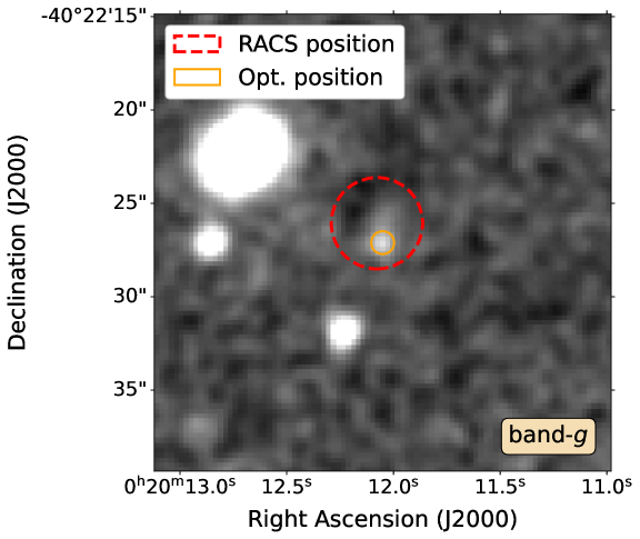
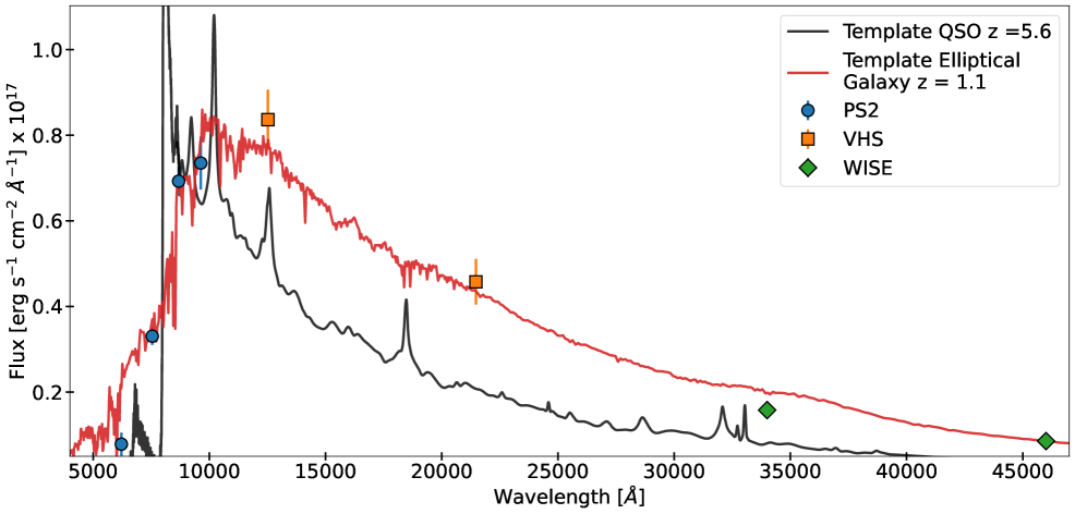
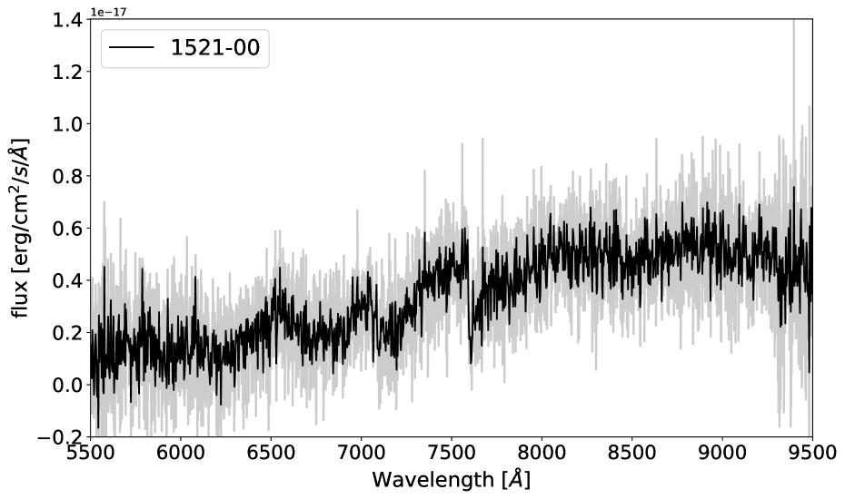
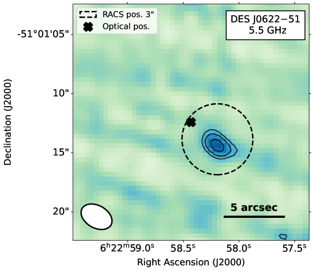
Figure 15: Top-left panel: Example of high-$z$ candidate selected based on the initial optical/IR selections from DES and catWISE, but then discarded after a visual inspection of its $g$-band image. Note that the image has been smoothed with a Gaussian filter in order to make the faint signals at the position of the optical source more evident. Top-right panel: Example of a selected candidate which was then discarded based on the NIR photometric points (from VHS). The black solid line is a template for high-$z$ quasars and the red solid line is a template for an elliptical galaxy. In this specific case, the source is likely an elliptical galaxy at $z\sim 1.1$. Bottom-left panel: Example of the LBT/MODS spectrum of a candidate (RACS J1521$-$00) not confirmed to be at high redshift. In this specific case, the target is likely a type M brown dwarf. The grey spectrum is at a resolution of $\sim$0.9 Å, whereas the black one is binned at $\sim$3.5 Å. Bottom-right panel: ATCA image at 5.5 GHz of RACS J0622$-$51, a candidate selected based on its optical/NIR colours and a radio association in the RACS-low survey within 3^′′ (dashed circle). The black cross shows the optical position of the high-$z$ candidate. The radio source detected with the ATCA revealed the RACS-low association to be spurious, with the radio source being $>10\sigma$ away from the optical counterpart, with $\sigma=0.24^{\prime\prime}$ the uncertainty on the ATCA position derived from the fit of the radio source. The black contours in the image are drawn at -3, 3, 3$\sqrt{2}$, 6 times the RMS of the image (RMS = 27 µJy beam^-1).

Target	R.A.	Dec.	drop	$S_{\rm 888MHz}$	mag$z$	drop	mag$z$–mag$W2$	dro	Telescope
	(deg)	(deg)	(Survey)	(mJy beam-1)	(mag AB)		(AB – Vega)	(arcsec)
RACS J0010$-$53	2.526012	$-$53.589526	$r$-drop (D)	1.2$\pm$0.4	20.84$\pm$0.04	1.64	3.35	1.47	VLT
RACS J0249$-$28	42.311270	$-$28.855045	$i$-drop (D)	5.1$\pm$0.5	20.83$\pm$0.03	1.23	3.09	2.01	VLT
RACS J0420$-$47	65.043381	$-$47.723408	$r$-drop (D)	10.3$\pm$0.7	21.22$\pm$0.04	1.62	3.63	2.13	VLT
RACS J0427$-$53	66.930894	$-$53.393840	$i$-drop (D)	3.6$\pm$0.6	20.04$\pm$0.01	1.08	3.20	1.47	VLT
RACS J0616$-$48	94.199469	$-$48.347094	$i$-drop (D)	2.1$\pm$0.8	21.24$\pm$0.03	1.39	3.37	2.76	VLT
RACS J0622$-$51	95.743477	$-$51.020087	$r$-drop (D)	1.9$\pm$0.7	20.74$\pm$0.03	1.82	3.72	2.71	ATCA∗
RACS J0905$-$10	136.262847	$-$10.426427	$r$-drop (P)	6.2$\pm$1.4	20.15$\pm$0.07	1.58	2.41	1.14	LBT
RACS J1521$-$00	230.377454	$-$0.300307	$r$-drop (P)	12.6$\pm$0.5	20.98$\pm$0.16	1.27	3.51	0.37	LBT
RACS J1552$-$29	238.041957	$-$29.255812	$r$-drop (P)	6.4$\pm$0.3	19.92$\pm$0.05	1.28	3.72	1.20	AAT
RACS J1557$-$18	239.321655	$-$18.041279	$r$-drop (P)	1.2$\pm$0.4	20.36$\pm$0.03	1.91	4.24	1.12	LBT
RACS J1614+14	243.735217	+14.315941	$r$-drop (P)	1.6$\pm$0.4	20.27$\pm$0.03	1.53	3.80	0.91	LBT
RACS J1722+29	260.728554	+29.108219	$i$-drop (P)	1.5$\pm$0.4	21.29$\pm$0.13	1.64	$<2.3$	1.30	LBT
RACS J1802+10	270.599597	+10.922134	$r$-drop (P)	6.1$\pm$0.7	20.27$\pm$0.06	1.58	3.89	1.02	LBT
RACS J2015$-$17	303.930440	$-$17.577126	$r$-drop (P)	1.6$\pm$0.3	20.96$\pm$0.09	1.82	3.90	0.27	TNG
RACS J2021$-$20	305.411544	$-$20.655044	$r$-drop (P)	2.5$\pm$0.5	20.67$\pm$0.04	1.52	3.61	1.23	AAT
RACS J2044$-$16	311.087282	$-$16.383996	$r$-drop (P)	1.5$\pm$0.4	20.70$\pm$0.06	1.74	$<1.7$	1.11	AAT
RACS J2103$-$40	315.773997	$-$40.697616	$r$-drop (D)	3.0$\pm$0.5	20.97$\pm$0.04	1.96	3.97	2.91	VLT
Not observed yet
RACS J0632$-$59	98.245905	$-$59.567634	$r$-drop (D)	1.2$\pm$0.4	21.01$\pm$0.04	1.81	2.93	1.14	–
RACS J0721+34	110.480455	+34.5776441	$i$-drop (P)	2.1$\pm$0.5	21.29$\pm$0.15	3.74	$<2.3$	1.42	–
RACS J0937$-$21	144.310777	$-$21.019468	$i$-drop (P)	1.0$\pm$0.3	20.82$\pm$0.03	1.22	$<1.8$	2.85	–
RACS J1536$-$28	234.204898	$-$28.4014139	$i$-drop (P)	1.8$\pm$0.3	21.04$\pm$0.09	1.53	4.62	2.05	–

Table 4: Properties, used for the selection, of the non-confirmed candidates. Col. (1, 2, 3): name and coordinates of the source; Col. (4): type of dropout and survey the source was selected from, in brackets; Col. (5): peak flux density at 888 MHz from the RACS-low source lists; Col. (6): $z$-band magnitude from DES or Pan-STARRS; Col. (7): dropout $r-i$ or $i-z$ depending on the type of dropout in Col. 4; Col. (8): $z-W2$ colour, where $z$ is in the AB system and $W2$ in the Vega one. In case of a non detection in the $W2$ filter, we assumed an upper limit of mag$W2$ = 19; Col. (9): radio-to-optical distance; Col. (10): telescope used for the identification. The ‘*’ indicates radio telescopes used to get more accurate position of the radio counterpart and discard the radio-optical association.

Appendix B Dedicated radio observations

In this section we list the dedicated radio observations available for the high-$z$ RACS sources that we used in order to build their radio spectra (see Fig. 11, 12 and 16). In particular, for $z>5$ sources already discussed in the literature, we considered the dedicated radio observations discussed in: Shao et al. (2020, 2022) for RACS J0131$-$03, RACS J0741+25, RACS J0836+00, RACS J1026+25, RACS J1034+20, RACS J1146+40 and RACS J1427+33; Gloudemans et al. (2023b) for RACS J0309+27 and RACS J2201+23; Keller et al. (2024) for RACS J1427+33; An et al. (2023) for RACS J1702+13.

In addition, we also performed observations for a sub-set of the newly identified $z>4.5$ radio quasars with the following radio telescopes radio telescopes (PI: Ighina): upgraded Giant Metrewave Radio Telescope (uGMRT) for RACS J0320$-$35 and RACS J0322$-$18 (project 42_001), MeerKAT for RACS J2252$-$51 (project DDT-20231128-LI-01) and ATCA (for 10 targets; projects C3477, C3535, C3601). The data reduction for the uGMRT and ATCA data-sets was performed similarly to Ighina et al. (2024b, a). Here we provide a short summary of the main steps.

uGMRT observations of RACS J0320$-$35 and RACS J0320$-$18 were performed using the GMRT wideband backend (GWB; Reddy et al. 2017 with a bandwidth of 200 MHz) in band-3 (centred at 400 MHz) and in band-4 (centred at 650 MHz). The data reduction was performed using the CAsa Pipeline-cum-Toolkit for Upgraded GMRT data REduction (CAPTURE; Kale & Ishwara-Chandra 2021) code by applying further flagging depending on the specific observation and by applying four cycles of phase self-calibration. For the imaging analysis, we adopted a robust parameter of 0.5 (i.e. a compromise between resolution and sensitivity).

ATCA observations were carried out at three different central frequencies: 2.1, 5.5 and 9 GHz (all with a bandwidth of 2 GHz). To process the data (calibration and imaging), we used the MIRIAD data-reduction package (Sault et al. 1995) following a standard reduction. We also applied 1-3 cycles of phase self-calibration to these data-sets, depending on the brightness of the objects in the filed of each target. For imaging, we adopted a robust parameter of 0.5.

Dedicated MeerKAT observations for RACS J2252$-$51 were performed on 2023 December 01-02-03 in three different bands: L (centred at 1.3 GHz), S0 (centred at 2.1 GHz) and S4 (centred at 3.1 GHz). We reduced the data using Oxkat (v0.4; Heywood 2020), where the Common Astronomy Software Applications (CASA; McMullin et al. 2007a) package and Tricolour (Hugo et al. 2022) were used for measurement sets splitting, cross-calibration, and flagging. CubiCal (Kenyon et al. 2018) was used for self-calibration, and Wsclean (Offringa et al. 2014) was used for continuum imaging. All processes were executed with Oxkat default settings.

For all these different observations (uGMRT, ATCA and MeerKAT) we performed a 2D Gaussian fit to the radio emission obtained in the final images using the CASA (McMullin et al. 2007b) software. We report in Tab. 6 the results of the fit for these new radio observations. We consider a further 5% error in the flux density estimates obtained, added in quadrature, to account for uncertainties related to the absolute flux scale and the reduction process.

Table 5: Best-fit flux estimated from the dedicated radio observations of a sub-set of sources within the RACS sample.

Source	Central Frequency	Flux	Flux error	Telescope
	(GHz)	(mJy)	mJy
RACS J0036$-$37	2.1	0.67	0.13	ATCA
	5.5	0.73	0.07	ATCA
	9.0	0.39	0.07	ATCA
RACS J0110$-$39	2.1	10.1	0.3	ATCA
	5.5	5.3	0.4	ATCA
	9.0	3.7	0.2	ATCA
RACS J0127$-$44	2.1	13.7	0.2	ATCA
	5.5	13.7	0.2	ATCA
	9.0	12.1	0.3	ATCA
RACS J0202$-$17	2.1	16.1	0.1	ATCA
	5.5	19.1	0.1	ATCA
	9.0	13.8	0.1	ATCA
RACS J0209$-$56	2.1	13.0	0.2	ATCA
	5.5	10.4	0.1	ATCA
	9.0	9.5	0.1	ATCA
RACS J0320$-$35	0.4	5.6	0.9	uGMRT
	0.65	4.0	0.2	uGMRT
	2.1	2.09	0.09	ATCA
	5.5	0.84	0.03	ATCA
	9.0	0.63	0.03	ATCA
RACS J0322$-$18	0.4	4.0	0.3	uGMRT
	0.65	2.5	0.1	uGMRT
	2.1	1.28	0.06	ATCA
	5.5	0.61	0.03	ATCA
	9.0	0.44	0.03	ATCA
RACS J1011$-$01	5.5	4.0	0.2	ATCA
	9.0	2.7	0.2	ATCA
RACS J1322$-$13	5.5	53.27	0.2	ATCA
	9.0	46.60	0.1	ATCA
RACS J1426$-$11	5.5	2.54	0.2	ATCA
	9.0	1.6	0.1	ATCA
RACS J2020$-$62	2.1	0.82	0.20	ATCA
	5.5	0.80	0.08	ATCA
	9.0	0.43	0.05	ATCA
RACS J2252$-$51	1.3	16.91	0.07	MeerKAT
	2.2	15.43	0.05	MeerKAT
	3.1	12.30	0.04	MeerKAT
	2.1	16.1	0.2	ATCA
	5.5	6.7	0.1	ATCA
	9.0	4.0	0.1	ATCA
	5.5	6.51	0.05	ATCA
	9.0	3.65	0.03	ATCA

Table 6: Flux densities derived from dedicated observations of a sub-sample of the RACS high-$z$ quasars. The errors reported here are the ones derived from the 2D Gaussian fit of the source in the given image and do not take the uncertainty in the flux scale calibration (assumed to be 5%) into account.

Appendix C Properties of the $z<5$ RACS quasars

In this section we report the multi-wavelength properties of the $z<5$ radio quasars identified from our selection, similarly to the ones reported in the main text for the well-defined sample at $z>5$. In particular, in Fig. 16 we show their radio spectra built from publicly available surveys (see Sec. 6) and dedicated observations (see Sec. B). Moreover, we also report their optical and radio luminosities, as well as radio spectral indices and R and $\tilde{\alpha}_{\rm ox}$ parameters in Tab. 18.

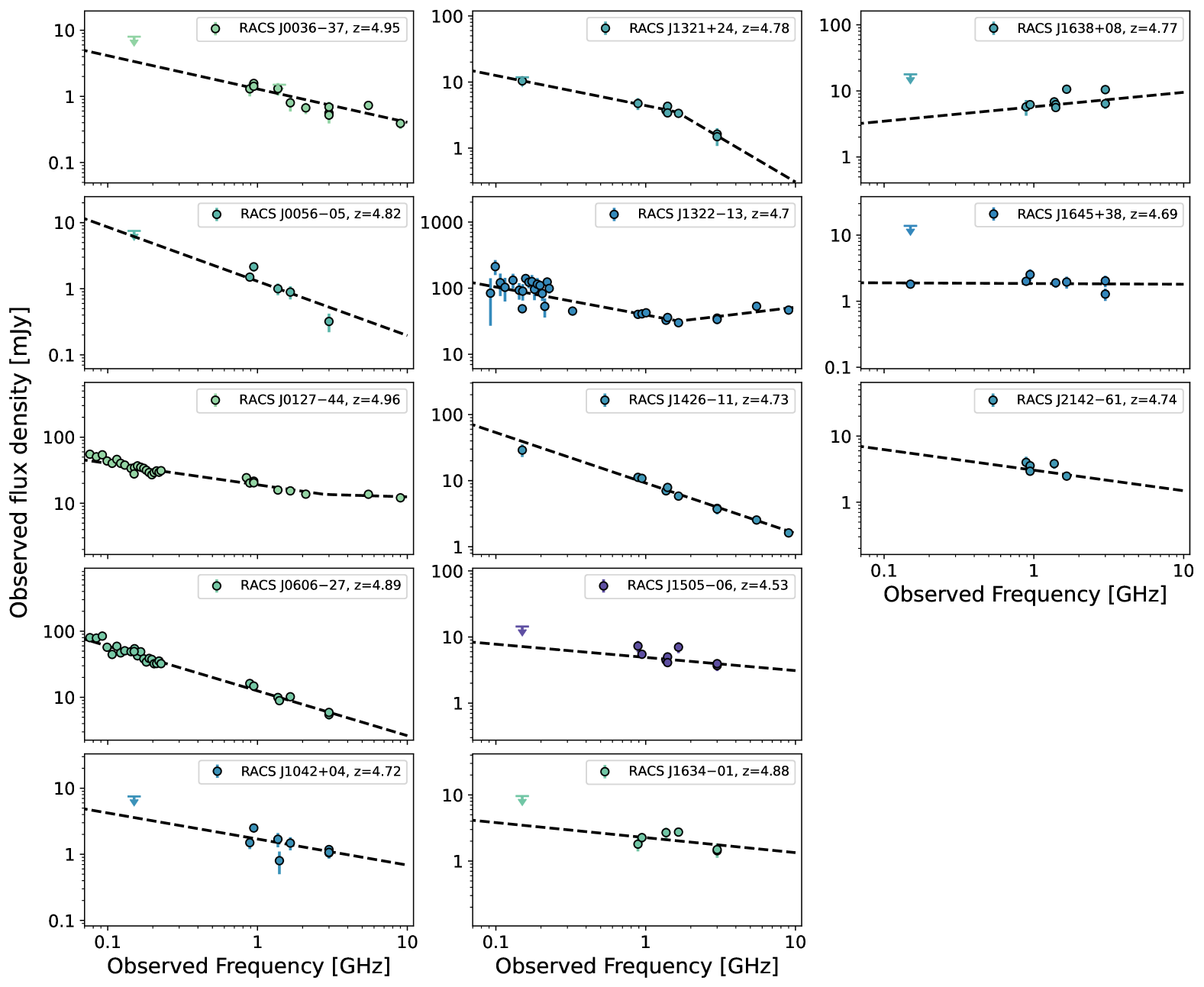
Figure 16: Radio spectra of the $4.5<z<5$ radio quasars discovered from RACS-low. The data-points are colour-coded based on their redshift (same scale of Fig. 6) and are mainly from public surveys with some sources having dedicated observations (see Tab. 6).

Table 7: Multi-wavelength properties of the $z<5$ RACS quasars.

Name	$z$	log(L${}_{2500\text{\AA }}$)	log(L${}_{4400\text{\AA }}$)	log(L5GHz)	log($\nu$L1.4GHz)	log(R)	${\alpha}_{\rm low}^{\rm r}$	${\alpha}_{\rm high}^{\rm r}$	${\nu}_{\rm break}$	$\tilde{\alpha}_{\rm ox}$
		(erg s-1 Hz-1)	(erg s-1 Hz-1)	(erg s-1 Hz-1)	(erg s-1)			GHz
RACS J0036$-$37	4.95	31.20$\pm$0.03	31.46$\pm$0.03	32.78$\pm$0.07	42.21$\pm$0.07	1.32$\pm$0.08	0.50 ${}_{-0.04}^{+0.04}$	–	–	$>1.03$
RACS J0056$-$05	4.82	30.80$\pm$0.04	31.03$\pm$0.04	32.77$\pm$0.09	42.38$\pm$0.09	1.74$\pm$0.10	0.82 ${}_{-0.01}^{+0.01}$	–	–	–
RACS J0127$-$44	4.96	30.95$\pm$0.03	30.99$\pm$0.04	33.94$\pm$0.07	43.26$\pm$0.07	2.95$\pm$0.08	0.32 ${}_{-0.14}^{+0.14}$	0.07 ${}_{-0.06}^{+0.06}$	2.82 ${}_{-0.49}^{+0.55}$	1.12$\pm$0.08
RACS J0606$-$27	4.89	31.16$\pm$0.03	31.41$\pm$0.03	33.77$\pm$0.07	43.29$\pm$0.07	2.36$\pm$0.08	0.68 ${}_{-0.11}^{+0.10}$	–	–	$>1.05$
RACS J1042+04	4.74	30.81$\pm$0.04	30.90$\pm$0.05	32.85$\pm$0.09	42.22$\pm$0.09	1.95$\pm$0.10	0.39 ${}_{-0.17}^{+0.14}$	–	–	$>0.94$
RACS J1321+24	4.78	30.81$\pm$0.04	30.90$\pm$0.05	33.28$\pm$0.07	42.68$\pm$0.07	2.38$\pm$0.09	0.46 ${}_{-0.01}^{+0.01}$	1.34 ${}_{-0.39}^{+0.39}$	1.60 ${}_{-0.33}^{+0.33}$	–
RACS J1322$-$13	4.70	31.05$\pm$0.03	31.22$\pm$0.04	34.22$\pm$0.07	43.59$\pm$0.07	3.01$\pm$0.08	0.42 ${}_{-0.02}^{+0.03}$	$-$0.27 ${}_{-0.03}^{+0.03}$	1.66 ${}_{-0.08}^{+0.10}$	1.02$\pm$0.03
RACS J1426$-$11	4.73	30.80$\pm$0.04	30.84$\pm$0.07	33.61$\pm$0.07	43.59$\pm$0.07	2.77$\pm$0.10	0.76 ${}_{-0.04}^{+0.04}$	–	–	$>0.97$
RACS J1505$-$06	4.53	30.93$\pm$0.04	31.07$\pm$0.04	33.27$\pm$0.09	42.53$\pm$0.09	2.20$\pm$0.10	0.20 ${}_{-0.04}^{+0.03}$	–	–	$>1.05$
RACS J1634$-$01	4.88	31.10$\pm$0.03	31.13$\pm$0.04	32.99$\pm$0.09	42.26$\pm$0.09	1.86$\pm$0.10	0.23 ${}_{-0.04}^{+0.04}$	–	–	–
RACS J1638+08	4.77	31.10$\pm$0.03	31.31$\pm$0.03	33.35$\pm$0.10	42.38$\pm$0.10	2.04$\pm$0.11	$-$0.22 ${}_{-0.09}^{+0.08}$	–	–	–
RACS J1645+38	4.69	30.74$\pm$0.04	30.79$\pm$0.05	32.86$\pm$0.07	42.01$\pm$0.07	2.07$\pm$0.09	0.01 ${}_{-0.01}^{+0.01}$	–	–	–
RACS J2142$-$61	4.74	31.31$\pm$0.03	31.43$\pm$0.03	33.10$\pm$0.12	42.42$\pm$0.12	1.67$\pm$0.12	0.31 ${}_{-0.02}^{+0.02}$	–	–	$>1.06$

References

- AAO software team (2015) AAO software team. 2015, 2dfdr: Data reduction software, Astrophysics Source Code Library, record ascl:1505.015
- Abbott et al. (2018) Abbott, T. M. C., Abdalla, F. B., Allam, S., et al. 2018, ApJS, 239, 18
- Abbott et al. (2021) Abbott, T. M. C., Adamów, M., Aguena, M., et al. 2021, ApJS, 255, 20
- Abdurro’uf et al. (2022) Abdurro’uf, Accetta, K., Aerts, C., et al. 2022, ApJS, 259, 35
- Akaike (1974) Akaike, H. 1974, IEEE Transactions on Automatic Control, 19, 716
- An & Romani (2020) An, H. & Romani, R. W. 2020, ApJ, 904, 27
- An et al. (2023) An, T., Wang, A., Liu, Y., et al. 2023, MNRAS, 519, 4047
- Arnaud (1996) Arnaud, K. A. 1996, in Astronomical Society of the Pacific Conference Series, Vol. 101, Astronomical Data Analysis Software and Systems V, ed. G. H. Jacoby & J. Barnes, 17
- Bañados et al. (2018) Bañados, E., Carilli, C., Walter, F., et al. 2018, ApJ, 861, L14
- Bañados et al. (2021) Bañados, E., Mazzucchelli, C., Momjian, E., et al. 2021, ApJ, 909, 80
- Bañados et al. (2025) Bañados, E., Momjian, E., Connor, T., et al. 2025, Nature Astronomy, 9, 293
- Bañados et al. (2023) Bañados, E., Schindler, J.-T., Venemans, B. P., et al. 2023, ApJS, 265, 29
- Bañados et al. (2016) Bañados, E., Venemans, B. P., Decarli, R., et al. 2016, ApJS, 227, 11
- Bañados et al. (2014) Bañados, E., Venemans, B. P., Morganson, E., et al. 2014, AJ, 148, 14
- Bañados et al. (2015) Bañados, E., Venemans, B. P., Morganson, E., et al. 2015, ApJ, 804, 118
- Barvainis et al. (2005) Barvainis, R., Lehár, J., Birkinshaw, M., Falcke, H., & Blundell, K. M. 2005, ApJ, 618, 108
- Becker et al. (1995) Becker, R. H., White, R. L., & Helfand, D. J. 1995, ApJ, 450, 559
- Behiri et al. (2025) Behiri, M., Mahony, E., Sadler, E., et al. 2025, arXiv e-prints, arXiv:2503.10811
- Belladitta et al. (2022) Belladitta, S., Caccianiga, A., Diana, A., et al. 2022, A&A, 660, A74
- Belladitta et al. (2023) Belladitta, S., Moretti, A., Caccianiga, A., et al. 2023, A&A, 669, A134
- Belladitta et al. (2019) Belladitta, S., Moretti, A., Caccianiga, A., et al. 2019, A&A, 629, A68
- Belladitta et al. (2020) Belladitta, S., Moretti, A., Caccianiga, A., et al. 2020, A&A, 635, L7
- Blandford et al. (2019) Blandford, R., Meier, D., & Readhead, A. 2019, ARA&A, 57, 467
- Burnham (2002) Burnham, Kenneth P., A. D. R. 2002, Model Selection and Multimodel Inference (London: Springer)
- Buzzoni et al. (1984) Buzzoni, B., Delabre, B., Dekker, H., et al. 1984, The Messenger, 38, 9
- Caccianiga et al. (2024) Caccianiga, A., Ighina, L., Moretti, A., et al. 2024, A&A, 684, A98
- Caccianiga et al. (2019) Caccianiga, A., Moretti, A., Belladitta, S., et al. 2019, MNRAS, 484, 204
- Calistro Rivera et al. (2017) Calistro Rivera, G., Williams, W. L., Hardcastle, M. J., et al. 2017, MNRAS, 469, 3468
- Capetti & Balmaverde (2024) Capetti, A. & Balmaverde, B. 2024, A&A, 689, A174
- Carilli et al. (2002) Carilli, C. L., Gnedin, N. Y., & Owen, F. 2002, ApJ, 577, 22
- Carilli et al. (2010) Carilli, C. L., Wang, R., Fan, X., et al. 2010, ApJ, 714, 834
- Carnall et al. (2015) Carnall, A. C., Shanks, T., Chehade, B., et al. 2015, MNRAS, 451, L16
- Carvajal et al. (2023) Carvajal, R., Matute, I., Afonso, J., et al. 2023, A&A, 679, A101
- Cash (1979) Cash, W. 1979, ApJ, 228, 939
- Chambers et al. (2016) Chambers, K. C., Magnier, E. A., Metcalfe, N., et al. 2016, eprint arXiv:1612.05560 [arXiv:1612.05560]
- Ciardi et al. (2013) Ciardi, B., Labropoulos, P., Maselli, A., et al. 2013, MNRAS, 428, 1755
- Condon et al. (1998) Condon, J. J., Cotton, W. D., Greisen, E. W., et al. 1998, AJ, 115, 1693
- Connor et al. (2024) Connor, T., Bañados, E., Cappelluti, N., & Foord, A. 2024, Universe, 10, 227
- Connor et al. (2021) Connor, T., Bañados, E., Stern, D., et al. 2021, ApJ, 911, 120
- Coppejans et al. (2016) Coppejans, R., Frey, S., Cseh, D., et al. 2016, MNRAS, 463, 3260
- Dallacasa et al. (2000) Dallacasa, D., Stanghellini, C., Centonza, M., & Fanti, R. 2000, A&A, 363, 887
- De Breuck et al. (2002) De Breuck, C., Tang, Y., de Bruyn, A. G., Röttgering, H., & van Breugel, W. 2002, A&A, 394, 59
- Deka et al. (2024) Deka, P. P., Gupta, N., Jagannathan, P., et al. 2024, ApJS, 270, 33
- Dey et al. (2019) Dey, A., Schlegel, D. J., Lang, D., et al. 2019, AJ, 157, 168
- Diana et al. (2022) Diana, A., Caccianiga, A., Ighina, L., et al. 2022, MNRAS, 511, 5436
- Driessen et al. (2024) Driessen, L. N., Pritchard, J., Murphy, T., et al. 2024, PASA, 41, e084
- Driver et al. (2011) Driver, S. P., Hill, D. T., Kelvin, L. S., et al. 2011, MNRAS, 413, 971
- Drouart & Falkendal (2018a) Drouart, G. & Falkendal, T. 2018a, MNRAS, 477, 4981
- Drouart & Falkendal (2018b) Drouart, G. & Falkendal, T. 2018b, MrMoose: Multi-Resolution Multi-Object/Origin Spectral Energy distribution fitting procedure, Astrophysics Source Code Library, record ascl:1809.015
- Drouart et al. (2020) Drouart, G., Seymour, N., Galvin, T. J., et al. 2020, PASA, 37, e026
- Duchesne et al. (2024) Duchesne, S. W., Grundy, J. A., Heald, G. H., et al. 2024, PASA, 41, e003
- Duchesne et al. (2025) Duchesne, S. W., Ross, K., Thomson, A. J. M., et al. 2025, arXiv e-prints, arXiv:2501.04978
- Duchesne et al. (2023) Duchesne, S. W., Thomson, A. J. M., Pritchard, J., et al. 2023, PASA, 40, e034
- Edge et al. (2013) Edge, A., Sutherland, W., Kuijken, K., et al. 2013, The Messenger, 154, 32
- Eisenhardt et al. (2020) Eisenhardt, P. R. M., Marocco, F., Fowler, J. W., et al. 2020, ApJS, 247, 69
- Elston et al. (2006) Elston, R. J., Gonzalez, A. H., McKenzie, E., et al. 2006, ApJ, 639, 816
- Euclid Collaboration et al. (2022) Euclid Collaboration, Scaramella, R., Amiaux, J., et al. 2022, A&A, 662, A112
- Fabian (2012) Fabian, A. C. 2012, ARA&A, 50, 455
- Fan et al. (2023) Fan, X., Bañados, E., & Simcoe, R. A. 2023, ARA&A, 61, 373
- Fan et al. (2001) Fan, X., Narayanan, V. K., Lupton, R. H., et al. 2001, AJ, 122, 2833
- Fan et al. (1999a) Fan, X., Strauss, M. A., Gunn, J. E., et al. 1999a, ApJ, 526, L57
- Fan et al. (2003) Fan, X., Strauss, M. A., Schneider, D. P., et al. 2003, AJ, 125, 1649
- Fan et al. (2000) Fan, X., Strauss, M. A., Schneider, D. P., et al. 2000, AJ, 119, 1
- Fan et al. (1999b) Fan, X., Strauss, M. A., Schneider, D. P., et al. 1999b, AJ, 118, 1
- Franzen et al. (2021) Franzen, T. M. O., Hurley-Walker, N., White, S. V., et al. 2021, PASA, 38, e014
- Freudling et al. (2013) Freudling, W., Romaniello, M., Bramich, D. M., et al. 2013, A&A, 559, A96
- Frey et al. (2024) Frey, S., Zhang, Y., Perger, K., et al. 2024, A&A, 681, L12
- Fruscione et al. (2006) Fruscione, A., McDowell, J. C., Allen, G. E., et al. 2006, in Society of Photo-Optical Instrumentation Engineers (SPIE) Conference Series, Vol. 6270, Society of Photo-Optical Instrumentation Engineers (SPIE) Conference Series, ed. D. R. Silva & R. E. Doxsey, 62701V
- Furlanetto et al. (2006) Furlanetto, S. R., Oh, S. P., & Briggs, F. H. 2006, Phys. Rep, 433, 181
- Gargiulo et al. (2022) Gargiulo, A., Fumana, M., Bisogni, S., et al. 2022, MNRAS, 514, 2902
- Garmire et al. (2003) Garmire, G. P., Bautz, M. W., Ford, P. G., Nousek, J. A., & Ricker, George R., J. 2003, in Society of Photo-Optical Instrumentation Engineers (SPIE) Conference Series, Vol. 4851, X-Ray and Gamma-Ray Telescopes and Instruments for Astronomy., ed. J. E. Truemper & H. D. Tananbaum, 28–44
- Ghisellini (2015) Ghisellini, G. 2015, Journal of High Energy Astrophysics, 7, 163
- Ghisellini et al. (2010) Ghisellini, G., Della Ceca, R., Volonteri, M., et al. 2010, MNRAS, 405, 387
- Ghisellini et al. (2013) Ghisellini, G., Haardt, F., Della Ceca, R., Volonteri, M., & Sbarrato, T. 2013, MNRAS, 432, 2818
- Ghisellini et al. (2014) Ghisellini, G., Sbarrato, T., Tagliaferri, G., et al. 2014, MNRAS, 440, L111
- Gilli et al. (2019) Gilli, R., Mignoli, M., Peca, A., et al. 2019, A&A, 632, A26
- Gloudemans et al. (2023a) Gloudemans, A. J., Callingham, J. R., Duncan, K. J., et al. 2023a, A&A, 678, A161
- Gloudemans et al. (2021) Gloudemans, A. J., Duncan, K. J., Röttgering, H. J. A., et al. 2021, A&A, 656, A137
- Gloudemans et al. (2022) Gloudemans, A. J., Duncan, K. J., Saxena, A., et al. 2022, A&A, 668, A27
- Gloudemans et al. (2023b) Gloudemans, A. J., Saxena, A., Intema, H., et al. 2023b, A&A, 678, A128
- Gloudemans et al. (2025) Gloudemans, A. J., Sweijen, F., Morabito, L. K., et al. 2025, ApJ, 980, L8
- Gordon et al. (2020) Gordon, Y. A., Boyce, M. M., O’Dea, C. P., et al. 2020, Research Notes of the American Astronomical Society, 4, 175
- Gürkan et al. (2022) Gürkan, G., Prandoni, I., O’Brien, A., et al. 2022, MNRAS, 512, 6104
- Hale et al. (2021) Hale, C. L., McConnell, D., Thomson, A. J. M., et al. 2021, PASA, 38, e058
- Hardcastle & Croston (2020) Hardcastle, M. J. & Croston, J. H. 2020, New A Rev., 88, 101539
- Harwood et al. (2013) Harwood, J. J., Hardcastle, M. J., Croston, J. H., & Goodger, J. L. 2013, MNRAS, 435, 3353
- Heywood (2020) Heywood, I. 2020, oxkat: Semi-automated imaging of MeerKAT observations, Astrophysics Source Code Library, record ascl:2009.003
- HI4PI Collaboration et al. (2016) HI4PI Collaboration, Ben Bekhti, N., Flöer, L., et al. 2016, A&A, 594, A116
- Hugo et al. (2022) Hugo, B. V., Perkins, S., Merry, B., Mauch, T., & Smirnov, O. M. 2022, in Astronomical Society of the Pacific Conference Series, Vol. 532, Astronomical Data Analysis Software and Systems XXX, ed. J. E. Ruiz, F. Pierfedereci, & P. Teuben, 541
- Hurley-Walker et al. (2017) Hurley-Walker, N., Callingham, J. R., Hancock, P. J., et al. 2017, MNRAS, 464, 1146
- Hurley-Walker et al. (2022) Hurley-Walker, N., Galvin, T. J., Duchesne, S. W., et al. 2022, PASA, 39, e035
- Ighina et al. (2021) Ighina, L., Belladitta, S., Caccianiga, A., et al. 2021, A&A, 647, L11
- Ighina et al. (2023) Ighina, L., Caccianiga, A., Moretti, A., et al. 2023, MNRAS, 519, 2060
- Ighina et al. (2019) Ighina, L., Caccianiga, A., Moretti, A., et al. 2019, MNRAS, 489, 2732
- Ighina et al. (2024a) Ighina, L., Caccianiga, A., Moretti, A., et al. 2024a, A&A, 692, A241
- Ighina et al. (2024b) Ighina, L., Caccianiga, A., Moretti, A., et al. 2024b, A&A, 687, A242
- Ighina et al. (2022a) Ighina, L., Leung, J. K., Broderick, J. W., et al. 2022a, A&A, 663, A73
- Ighina et al. (2022b) Ighina, L., Moretti, A., Tavecchio, F., et al. 2022b, A&A, 659, A93
- Intema et al. (2017) Intema, H. T., Jagannathan, P., Mooley, K. P., & Frail, D. A. 2017, A&A, 598, A78
- Ivezić et al. (2019) Ivezić, Ž., Kahn, S. M., Tyson, J. A., et al. 2019, ApJ, 873, 111
- Jiang et al. (2008) Jiang, L., Fan, X., Annis, J., et al. 2008, AJ, 135, 1057
- Jolley & Kuncic (2008) Jolley, E. J. D. & Kuncic, Z. 2008, MNRAS, 386, 989
- Jolley et al. (2009) Jolley, E. J. D., Kuncic, Z., Bicknell, G. V., & Wagner, S. 2009, MNRAS, 400, 1521
- Kale & Ishwara-Chandra (2021) Kale, R. & Ishwara-Chandra, C. H. 2021, Experimental Astronomy, 51, 95
- Kappes et al. (2022) Kappes, A., Burd, P. R., Kadler, M., et al. 2022, A&A, 663, A44
- Keim et al. (2019) Keim, M. A., Callingham, J. R., & Röttgering, H. J. A. 2019, A&A, 628, A56
- Keller et al. (2024) Keller, P. M., Thyagarajan, N., Kumar, A., Kanekar, N., & Bernardi, G. 2024, MNRAS, 528, 5692
- Kellermann et al. (1989) Kellermann, K. I., Sramek, R., Schmidt, M., Shaffer, D. B., & Green, R. 1989, AJ, 98, 1195
- Kenyon et al. (2018) Kenyon, J. S., Smirnov, O. M., Grobler, T. L., & Perkins, S. J. 2018, MNRAS, 478, 2399
- Khorunzhev et al. (2021) Khorunzhev, G. A., Meshcheryakov, A. V., Medvedev, P. S., et al. 2021, Astronomy Letters, 47, 123
- Krezinger et al. (2024) Krezinger, M., Frey, S., Perger, K., et al. 2024, MNRAS, 530, 4614
- Lacy et al. (2020) Lacy, M., Baum, S. A., Chandler, C. J., et al. 2020, Publications of the Astronomical Society of the Pacific, 132, 035001
- Lai et al. (2023) Lai, S., Onken, C. A., Wolf, C., et al. 2023, MNRAS, 526, 3230
- Latif et al. (2024) Latif, M. A., Whalen, D. J., & Mezcua, M. 2024, MNRAS, 527, L37
- Li et al. (2021) Li, J.-T., Wang, F., Yang, J., et al. 2021, ApJ, 906, 135
- Liu et al. (2009) Liu, X., Song, H. G., & Cui, L. 2009, Astronomische Nachrichten, 330, 145
- Lusso & Risaliti (2016) Lusso, E. & Risaliti, G. 2016, ApJ, 819, 154
- Maiolino et al. (2024) Maiolino, R., Scholtz, J., Witstok, J., et al. 2024, Nature, 627, 59
- Mao et al. (2017) Mao, P., Urry, C. M., Marchesini, E., et al. 2017, ApJ, 842, 87
- Marocco et al. (2021) Marocco, F., Eisenhardt, P. R. M., Fowler, J. W., et al. 2021, ApJS, 253, 8
- Matsuoka et al. (2022) Matsuoka, Y., Iwasawa, K., Onoue, M., et al. 2022, ApJS, 259, 18
- Matsuoka et al. (2018a) Matsuoka, Y., Iwasawa, K., Onoue, M., et al. 2018a, ApJS, 237, 5
- Matsuoka et al. (2018b) Matsuoka, Y., Onoue, M., Kashikawa, N., et al. 2018b, Publications of the Astronomical Society of Japan, 70, S35
- Matsuoka et al. (2016) Matsuoka, Y., Onoue, M., Kashikawa, N., et al. 2016, ApJ, 828, 26
- Mauch et al. (2003) Mauch, T., Murphy, T., Buttery, H. J., et al. 2003, MNRAS, 342, 1117
- McConnell et al. (2020) McConnell, D., Hale, C. L., Lenc, E., et al. 2020, PASA, 37, e048
- McGreer et al. (2006) McGreer, I. D., Becker, R. H., Helfand, D. J., & White, R. L. 2006, ApJ, 652, 157
- McGreer et al. (2009) McGreer, I. D., Helfand, D. J., & White, R. L. 2009, AJ, 138, 1925
- McMahon et al. (2021) McMahon, R. G., Banerji, M., Gonzalez, E., et al. 2021, VizieR Online Data Catalog, II/367
- McMullin et al. (2007a) McMullin, J. P., Waters, B., Schiebel, D., Young, W., & Golap, K. 2007a, in Astronomical Society of the Pacific Conference Series, Vol. 376, Astronomical Data Analysis Software and Systems XVI, ed. R. A. Shaw, F. Hill, & D. J. Bell, 127
- McMullin et al. (2007b) McMullin, J. P., Waters, B., Schiebel, D., Young, W., & Golap, K. 2007b, in Astronomical Society of the Pacific Conference Series, Vol. 376, Astronomical Data Analysis Software and Systems XVI, ed. R. A. Shaw, F. Hill, & D. J. Bell, 127
- Medvedev et al. (2021) Medvedev, P., Gilfanov, M., Sazonov, S., Schartel, N., & Sunyaev, R. 2021, MNRAS, 504, 576
- Medvedev et al. (2020) Medvedev, P., Sazonov, S., Gilfanov, M., et al. 2020, MNRAS, 497, 1842
- Merloni et al. (2024) Merloni, A., Lamer, G., Liu, T., et al. 2024, A&A, 682, A34
- Miley & De Breuck (2008) Miley, G. & De Breuck, C. 2008, A&A Rev., 15, 67
- Mingaliev et al. (2012) Mingaliev, M. G., Sotnikova, Y. V., Torniainen, I., Tornikoski, M., & Udovitskiy, R. Y. 2012, A&A, 544, A25
- Morabito et al. (2016) Morabito, L. K., Deller, A. T., Röttgering, H., et al. 2016, MNRAS, 461, 2676
- Moretti et al. (2021) Moretti, A., Ghisellini, G., Caccianiga, A., et al. 2021, ApJ, 920, 15
- Morganson et al. (2012) Morganson, E., De Rosa, G., Decarli, R., et al. 2012, AJ, 143, 142
- Myers et al. (2003) Myers, S. T., Jackson, N. J., Browne, I. W. A., et al. 2003, MNRAS, 341, 1
- Nanni et al. (2022) Nanni, R., Hennawi, J. F., Wang, F., et al. 2022, MNRAS, 515, 3224
- Nanni et al. (2017) Nanni, R., Vignali, C., Gilli, R., Moretti, A., & Brandt, W. N. 2017, A&A, 603, A128
- Niida et al. (2020) Niida, M., Nagao, T., Ikeda, H., et al. 2020, ApJ, 904, 89
- Niu et al. (2025) Niu, Q., Li, Y., Xu, Y., Guo, H., & Zhang, X. 2025, ApJ, 978, 145
- Norris et al. (2021) Norris, R. P., Marvil, J., Collier, J. D., et al. 2021, PASA, 38, e046
- O’Dea & Saikia (2021) O’Dea, C. P. & Saikia, D. J. 2021, A&AR, 29, 3
- Offringa et al. (2014) Offringa, A. R., McKinley, B., Hurley-Walker, N., et al. 2014, MNRAS, 444, 606
- Onken et al. (2022) Onken, C. A., Wolf, C., Bian, F., et al. 2022, MNRAS, 511, 572
- Orienti & Dallacasa (2012) Orienti, M. & Dallacasa, D. 2012, MNRAS, 424, 532
- Orienti & Dallacasa (2014) Orienti, M. & Dallacasa, D. 2014, MNRAS, 438, 463
- Overzier (2016) Overzier, R. A. 2016, A&A Rev., 24, 14
- Overzier et al. (2009) Overzier, R. A., Guo, Q., Kauffmann, G., et al. 2009, MNRAS, 394, 577
- Padovani & Giommi (1995) Padovani, P. & Giommi, P. 1995, ApJ, 444, 567
- Polletta et al. (2007) Polletta, M., Tajer, M., Maraschi, L., et al. 2007, ApJ, 663, 81
- Reddy et al. (2017) Reddy, S. H., Kudale, S., Gokhale, U., et al. 2017, Journal of Astronomical Instrumentation, 6, 1641011
- Reed et al. (2019) Reed, S. L., Banerji, M., Becker, G. D., et al. 2019, MNRAS, 487, 1874
- Reed et al. (2015) Reed, S. L., McMahon, R. G., Banerji, M., et al. 2015, MNRAS, 454, 3952
- Reed et al. (2017) Reed, S. L., McMahon, R. G., Martini, P., et al. 2017, MNRAS, 468, 4702
- Ross et al. (2024) Ross, K., Hurley-Walker, N., Galvin, T. J., et al. 2024, PASA, 41, e054
- Sabater et al. (2021) Sabater, J., Best, P. N., Tasse, C., et al. 2021, A&A, 648, A2
- Sault et al. (1995) Sault, R. J., Teuben, P. J., & Wright, M. C. H. 1995, in Astronomical Society of the Pacific Conference Series, Vol. 77, Astronomical Data Analysis Software and Systems IV, ed. R. A. Shaw, H. E. Payne, & J. J. E. Hayes, 433
- Sbarrato et al. (2012) Sbarrato, T., Ghisellini, G., Nardini, M., et al. 2012, MNRAS, 426, L91
- Sbarrato et al. (2022) Sbarrato, T., Ghisellini, G., Tagliaferri, G., et al. 2022, A&A, 663, A147
- Shao et al. (2020) Shao, Y., Wagg, J., Wang, R., et al. 2020, A&A, 641, A85
- Shao et al. (2022) Shao, Y., Wagg, J., Wang, R., et al. 2022, A&A, 659, A159
- Shimwell et al. (2022) Shimwell, T. W., Hardcastle, M. J., Tasse, C., et al. 2022, A&A, 659, A1
- Shimwell et al. (2017) Shimwell, T. W., Röttgering, H. J. A., Best, P. N., et al. 2017, A&A, 598, A104
- Shimwell et al. (2019) Shimwell, T. W., Tasse, C., Hardcastle, M. J., et al. 2019, A&A, 622, A1
- Sotnikova et al. (2024) Sotnikova, Y., Mikhailov, A., Mufakharov, T., et al. 2024, Galaxies, 12, 25
- Sotnikova et al. (2021) Sotnikova, Y., Mikhailov, A., Mufakharov, T., et al. 2021, MNRAS, 508, 2798
- Spingola et al. (2020) Spingola, C., Dallacasa, D., Belladitta, S., et al. 2020, A&A, 643, L12
- Tasse et al. (2021) Tasse, C., Shimwell, T., Hardcastle, M. J., et al. 2021, A&A, 648, A1
- Tinti et al. (2005) Tinti, S., Dallacasa, D., de Zotti, G., Celotti, A., & Stanghellini, C. 2005, A&A, 432, 31
- Tody (1986) Tody, D. 1986, in Society of Photo-Optical Instrumentation Engineers (SPIE) Conference Series, Vol. 627, Instrumentation in astronomy VI, ed. D. L. Crawford, 733
- Tody (1993) Tody, D. 1993, in Astronomical Society of the Pacific Conference Series, Vol. 52, Astronomical Data Analysis Software and Systems II, ed. R. J. Hanisch, R. J. V. Brissenden, & J. Barnes, 173
- Uchiyama et al. (2022) Uchiyama, H., Yamashita, T., Nagao, T., et al. 2022, PASJ, 74, L27
- Vanden Berk et al. (2001) Vanden Berk, D. E., Richards, G. T., Bauer, A., et al. 2001, AJ, 122, 549
- Venemans et al. (2015) Venemans, B. P., Bañados, E., Decarli, R., et al. 2015, ApJ, 801, L11
- Venemans et al. (2013) Venemans, B. P., Findlay, J. R., Sutherland, W. J., et al. 2013, ApJ, 779, 24
- Vignali et al. (2005) Vignali, C., Brandt, W. N., Schneider, D. P., & Kaspi, S. 2005, AJ, 129, 2519
- Volonteri et al. (2021) Volonteri, M., Habouzit, M., & Colpi, M. 2021, Nature Reviews Physics, 3, 732
- Šoltinský et al. (2021) Šoltinský, T., Bolton, J. S., Hatch, N., et al. 2021, MNRAS, 506, 5818
- Šoltinský et al. (2025) Šoltinský, T., Kulkarni, G., Tendulkar, S. P., & Bolton, J. S. 2025, MNRAS, 537, 364
- Wachter et al. (1979) Wachter, K., Leach, R., & Kellogg, E. 1979, ApJ, 230, 274
- Wang et al. (2016) Wang, F., Wu, X.-B., Fan, X., et al. 2016, ApJ, 819, 24
- Wang et al. (2019) Wang, F., Yang, J., Fan, X., et al. 2019, ApJ, 884, 30
- Wayth et al. (2015) Wayth, R. B., Lenc, E., Bell, M. E., et al. 2015, PASA, 32, e025
- Wayth et al. (2018) Wayth, R. B., Tingay, S. J., Trott, C. M., et al. 2018, PASA, 35, e033
- Wenzl et al. (2021) Wenzl, L., Schindler, J.-T., Fan, X., et al. 2021, AJ, 162, 72
- Wolf et al. (2020) Wolf, C., Hon, W. J., Bian, F., et al. 2020, MNRAS, 491, 1970
- Wolf et al. (2021) Wolf, J., Nandra, K., Salvato, M., et al. 2021, A&A, 647, A5
- Wolf et al. (2024) Wolf, J., Salvato, M., Belladitta, S., et al. 2024, A&A, 691, A30
- Wu et al. (2013) Wu, J., Brandt, W. N., Miller, B. P., et al. 2013, ApJ, 763, 109
- Yang et al. (2023) Yang, J., Fan, X., Gupta, A., et al. 2023, ApJS, 269, 27
- Yang et al. (2017) Yang, J., Fan, X., Wu, X.-B., et al. 2017, AJ, 153, 184
- Yang et al. (2019) Yang, J., Wang, F., Fan, X., et al. 2019, AJ, 157, 236
- Yang et al. (2016) Yang, J., Wang, F., Wu, X.-B., et al. 2016, ApJ, 829, 33
- Ye et al. (2024) Ye, G., Zhang, H., & Wu, Q. 2024, ApJS, 275, 19
- Zuo et al. (2024) Zuo, Z., Zhu, S., Brandt, W. N., et al. 2024, MNRAS, 530, 360