Dynamical systems approach to Cold and Warm Inflation within slow-roll and beyond

Abstract

In this work, we systematically present a new dynamical systems approach to standard inflationary processes and their variants as constant-roll inflation. Using the techniques presented in our work one can in general investigate the attractor nature of the inflationary models in the phase space. We have compactified the phase space coordinates, wherever necessary, and regulated the nonlinear differential equations, constituting the autonomous system of equations defining the dynamical system, at the cost of a new redefined time variable which is a monotonic increasing function of the standard time coordinate. We have shown that in most of the relevant cases the program is executable although the two time coordinates may show different durations of cosmological events. If one wishes one can revert back to the cosmological time via an inverse transformation. The present work establishes a standard norm for studying dynamical as well as stability issues in any new inflationary system.

1 Introduction

Inflationary models have been pivotal in explaining the early universe’s rapid expansion and resolving several cosmological puzzles, such as the flatness and horizon problems [1, 2, 3, 4, 5, 6, 7]. In inflationary dynamics it is tacitly assumed that the very early universe do evolve in an inflationary phase after the initial singularity for a very brief period of time. In this case a question arises, what are the initial conditions which naturally drive the system towards inflation? As it is very difficult to specify some specific set of initial conditions in the very early universe with pin-point accuracy, the general consensus is to focus on a class of initial conditions which can give rise to inflation. If a wide region, in the set of initial conditions on phase space, leads to inflation, one can be sure that an inflation like phase was there after the initial cosmological singularity. The existence of such a large class of initial conditions shows that inflation is an attractor solution. A preliminary but interesting theory of attractor solution of cold inflation (CI) was presented in Ref. [8, 9, 10, 11, 12]. If a wide range of initial conditions can produce inflation, with all its constraints, then we say the attractor solution shows stability.

In general the stability issues about any system are best studied in the dynamical systems approach where one recasts all the dynamical equations of the system in the form of nonlinear, first order autonomous system of differential equations. The dynamical systems approach has emerged as a powerful tool in late-time cosmology, particularly for analyzing new classes of cosmological models [13, 14, 15, 16, 17, 18, 19, 20, 21, 22, 23, 24, 25, 26, 27, 28, 29, 30, 31]. In inflationary cosmology, one rarely use the full potential of the dynamical systems approach as we do not expect the system to have any stable fixed points during the inflationary regime. Moreover, a successful period of inflation ends in reheating the universe and the physics of reheating [32, 33, 34, 35] is different from the physics of slow-roll inflation. Consequently a dynamical system which models a slow-roll process will be unable to yield meaningful information near the end of inflation unless the equations are modified so that the reheating process is also included in the dynamical equations. It is practically impossible to describe the initiation of inflation and the reheating phase with the same set of dynamical equations and mostly the dynamical systems approach concentrates on the initial development of an inflationary system and the analysis can be extended approximately up to the graceful exit phase. In warm inflation (WI) one does not have a separate reheating phase and we expect that a dynamical systems approach in WI is more useful. A dynamical systems approach has some advantages, it is a very general method which has the potential to unravel the dynamical properties of any system unambiguously. If the dynamical systems approach can be used in conjunction with a wide class of initial conditions then we get a set of trajectories in the phase space showing the qualitative behavior of the system. Except giving an overall, qualitative phase space picture of inflationary dynamics one can also analyze any inflationary scenario in detail using the methods of dynamical systems. In this paper we have tried to posit a uniform dynamical systems viewpoint using which one can study any inflationary process.

Except cold inflationary paradigm we also have a radically different inflationary paradigm: the paradigm of warm inflation (WI) [36, 37, 38, 39, 40, 41, 42, 43, 44, 45, 46, 47, 48, 49, 50, 51, 52]. In this paradigm, inflation happens due to the vacuum energy of the inflaton but the inflaton does decay to radiation during inflation and consequently the fluctuations produced by WI are thermal in nature. Warm inflation is more dynamically constrained, than the simple CI models, as in these case the radiation produced from the decay of inflaton can produce a dynamical thermal equilibrium as a result of which the radiation bath can have a temperature $T$. The dynamical constraints arises from multiple requirements:

• firstly, the requirement of successful inflation when inflaton energy inflates the system and simultaneously decays to radiation.

• The second requirement of maintaining a stable temperature $T$ during the inflationary process.

• The third requirement to maintain $T$ greater than the Hubble parameter during WI.

This last condition is essential for producing thermal fluctuations. Few previous authors have studied the dynamical systems approach and stability issues in WI [53, 54, 55, 56, 57, 58, 59, 60]. In the present work we generalize the previous techniques used by these authors and try to give new directions for the qualitative phase space study of WI. We have shown the attractor nature of WI where the dynamical system is highly constrained by the dynamical equilibrium requirements of the radiation bath. In general if one is purely interested in WI dynamics for a particular initial condition, then one may not use the constraints imposed by the equilibrium of the radiation bath because in slow-roll regime the variation of the temperature of the bath is relatively small during the inflationary period. In our case we produce the phase space trajectories of the system for various possible initial conditions: all of these trajectories may not be undergoing a slow-roll process. To differentiate the phase space trajectories which evolve through a thermalized phase and non-thermalized phase we have explicitly shown how one can formulate the constrained WI dynamical system.

Closely related to the above two main modern paradigms of inflationary dynamics are some new variants. These variants are all some forms of CI or WI but they differ from the canonical models by the scalar field rolling condition. One of these variants are constant-roll cold inflation (CRCI) [61, 62, 63, 64, 65, 66, 67, 68, 69, 70, 71, 72, 73, 74, 75, 76, 77], which is a variant of CI where the slow-roll (SR) condition of the scalar field is changed to the constant-roll condition. In general inflationary dynamics is specified by some rolling conditions and one of these conditions are related to the value of $\ddot{\phi}/(H\dot{\phi})$ where $\phi$ represents the inflaton field and $H$ is the Hubble parameter during inflation. The dot represent derivatives with respect to cosmological time. In the slow-roll regime this ratio tends to zero, whereas in the constant-roll regime this ratio remains a constant. The constant-roll (CR) condition restricts the inflationary system although it is known that it remains an attractor solution near the SR limit. In this work we will verify this claim and show how the attractor solution in CRCI gets modified from the attractor solution in CI. We will also show that in CRCI there will be some dynamical evolutions where an accelerated expansion phase, like the inflation phase, goes on inflating and cannot come out of the inflationary process through graceful exit.

Building on the concepts of (CRCI) and WI, researchers have proposed models of constant-roll warm inflation (CRWI) [78, 79]. In this variant, one studies warm inflation after imposing the constant-roll condition, i.e. demanding $\ddot{\phi}/(H\dot{\phi})$ to be a constant. CRWI is a highly constrained framework, as it inherits the requirement of dynamical equilibrium in the radiation bath from warm inflation (WI), while the constant-roll condition further restricts the dynamics of the system. The constant-roll (CR) condition imposes significant restrictions on the CR variants of both cold and warm inflation, permitting only a narrow class of scalar field potentials to sustain these inflationary phases—unlike standard cold or warm inflation, which can be realized with a broad range of potentials [80]. These constraints render a substantial portion of the phase space inaccessible to the dynamical system. Nevertheless, the attractor behavior of CRWI can still be visualized within the available phase space. In this work, we have presented the dynamics of such systems and have thoroughly analyzed the structure of the phase space for various values of the CR parameters.

In this paper, we have independently presented the dynamical analysis for each type of inflation discussed, allowing for a direct comparison of how different inflationary conditions influence the phase space dynamics. For the first time, a unified framework based on dynamical systems theory has been employed to study the various forms of inflation. We have successfully applied compactified phase space techniques and addressed ill-defined autonomous equations through a redefinition of time—methods that are novel in the context of inflationary dynamics. An exception is made in the case of CRCI, where the dynamical phase space is effectively one-dimensional. In such cases, a conventional autonomous system analysis offers limited insight. Therefore, for CRCI, we have adopted an alternative approach using stream plots of the phase space variables in a two-dimensional plane.

The material in this paper is organized as follows. In the next section 2, we briefly introduce the fundamentals of dynamical systems theory and apply it to analyze the phase space dynamics in cold inflation (CI). In section 3, we discuss the dynamics of CRCI for various values of the constant-roll parameter. Section 4 presents the phase space analysis for warm inflation (WI), wherein we compactify the phase space and regulate the dynamical system through a redefinition of time. In section 5, we extend the dynamical systems analysis to the constant-roll warm inflation (CRWI) case for different values of the constant-roll parameter. Finally, we summarize our approach and highlight the key findings regarding inflationary dynamics in the concluding section 6.

2 A brief introduction to the theory of dynamical systems and its application to the standard slow-roll cold inflation model

In this section we specify the conventions and notations used in this paper. Initially we specify the mathematical principles, related to the dynamical systems approach, which are used to analyze the various inflationary cases.

In both Cold and Warm Inflation, the background evolution is determined by the flat Friedmann-Lemaitre-Robertson-Walker (FLRW) metric described by the line element:

$$ds^{2}=dt^{2}-a(t)^{2}d\mathbf{x}^{2},$$ (2.1)

where $t$ is the cosmic time, $a(t)$ is the scale-factor of the universe, and $\mathbf{x}$ represents the spatial coordinates $(x,y,z)$. The fundamental dynamical equations governing a cold inflationary system consist of the Friedmann equations and the Klein–Gordon equation for the inflaton field, formulated in the FLRW background. In the case of warm inflation, the presence of a subdominant yet non-negligible radiation fluid—coupled to the inflaton field—necessitates the inclusion of the radiation fluid’s evolution equation as part of the dynamical system. To apply the dynamical systems approach, it is customary to recast the equations into an autonomous system using suitably defined phase space variables. These variables are chosen to ensure that the phase space has the minimal possible dimensionality and that all quantities involved are dimensionless. In our analysis, we reparametrize the cosmic time $t$ either using a dimensionless time variable $t^{\prime}$ in certain cases, or by the number of $e$-folds, defined via $dN=H\,dt$, where $H\equiv\dot{a}/a$ is the Hubble parameter.

In general, the phase space of a system can be either one-dimensional or higher-dimensional, depending on the number of independent dynamical variables required to construct a closed autonomous system of equations. For an $n$-dimensional phase space—corresponding to a cosmological system with $n$ independent dynamical variables—the first Friedmann equation, which involves the square of the Hubble parameter and various energy densities, always yields a constraint equation of the form:

$$f(x_{1},x_{2},\cdots,x_{n})=0\,,$$ (2.2)

where $(x_{1},x_{2},\cdot,\cdot,\cdot)$ are the phase space variables (not to confuse with the spatial coordinates $\mathbf{x}$ in Eq. (2.1)) and $f(x_{1},x_{2},x_{3},\cdot\cdot,x_{n})$ is an arbitrary function of these variables. The above constraint equation characterizes the topological structure of the phase space for the cosmological system. In such cases, the autonomous system of equations is typically written in the form:

$$\dot{x}_{1} = f_{1}(x_{1},x_{2},\cdots,x_{n})\,,$$

$$\dot{x}_{2} = f_{2}(x_{1},x_{2},\cdots,x_{n})\,,$$

$$\vdots$$

$$\dot{x}_{n} = f_{n}(x_{1},x_{2},\cdots,x_{n})\,,$$ (2.3)

where the overdots specify a derivative with respect to either $t^{\prime}$ or $N$, which are both dimensionless. Here the functions $f_{j}(x_{1},x_{2},\cdots,x_{n})$ (where $j=1,2,\cdots,n$) are in general nonlinear functions of the variables. The form of these functions are obtained from the actual dynamical equations of the system. The critical points (or fixed points) of the above system of equations are obtained for points $x_{c,k}\equiv(x_{1,k}^{*},x_{2,k}^{*},\cdots,x_{n,k}^{*})$ ($k=1,2,\cdots,m$ where $m$ represents the number of critical points) for which

$$\dot{x}_{1}=\dot{x}_{2}=\cdots=\dot{x}_{n}=0\,.$$

The condition may be satisfied for multiple points in the phase space and all those points ($x_{c,i}$) specify fixed points of the dynamical system.

The stability of the fixed points is determined by linearizing the right-hand side of the autonomous system around each fixed point and constructing the corresponding Jacobian matrix. This Jacobian is an $n\times n$ matrix, where $n$ is the dimensionality of the phase space. The elements of the Jacobian matrix, for the $k$th fixed point, are given by:

$$J^{(k)}_{ij}=\left.\dfrac{\partial\dot{x}_{i}}{\partial x_{j}}\right|_{x_{c,k}}.$$ (2.4)

After constructing the Jacobian matrix, the eigenvalues of the matrix can be computed. The stability of the fixed points is inferred from the sign of the real parts of these eigenvalues:

• If all the real parts of the eigenvalues are negative, the corresponding fixed point is stable.

• If all the real parts are positive, the fixed point is unstable.

• If the real parts have mixed signs, the fixed point is a saddle point.

• If any real part vanishes, the standard linearization technique cannot determine the nature of the fixed point.

In cases where the real part vanishes, one can apply the center manifold theorem or numerically evolve the system around the critical points [14]. Note that in some cases, the stability of certain fixed points is indeterminate using the linearization method. For such cases, one has to rely on numerical evolution of the system to assess their stability. If the dynamical variables converge to the fixed point coordinates after numerically evolving the system around these critical points, the corresponding fixed point is deemed stable.

Though, the above mentioned scheme of finding the trajectories of the dynamical system and the fixed points works well for many systems, there are a few exceptions, such as

1. when the phase space topology, as defined by Eq. (2.2), is noncompact. In such cases, the dynamical variables can attain arbitrarily large values, resulting in an unbounded phase space. Consequently, fixed points located at infinity cannot be captured using the standard dynamical systems approach.

2. When some of the autonomous equations in the system become singular. This occurs when certain functions $f_{i}(x_{1},x_{2},\cdots,x_{n})$ (as defined in Eqs. (2.3)) diverge for finite, physically permissible values of the phase space variables. A common example arises from terms involving inverse powers, such as $1/x_{i}$, which render the equations ill-defined at $x_{i}=0$.

Remedies to tackle such pathological cases in dynamical analysis have been suggested in [15, 16]. In brief, to tackle the noncompactness of the phase space, one can suitably map the phase space variables in terms of other dynamical variables which varies in a compact range adopting the most conventional one called Poincarè technique [81, 82]. One then rewrites the autonomous equations in terms of the new dynamical variables of a compact phase space. We will see later that such situations arise in many inflationary dynamics, including the simplest case of slow-roll cold inflation. On the other hand, to deal with the divergences appearing in the autonomous equations, it is customary to suitably redefine $t^{\prime}$ or $N$ to get rid of the infinities. We will exploit such methods when we will deal with the dynamics of Warm Inflation in Sec. 4.

It is a common lore that inflationary trajectories in the phase space of its dynamical system often shows an attractor behaviour, which means that given a wide range of initial conditions of the dynamical variables the inflationary trajectories tend towards a specific region of the phase space (often tends toward and evolves around a fixed point). Our main aim would be to recognize such attractor solutions both in cold and warm inflation with slow-roll as well as constant-roll dynamics.

2.1 Dynamical analysis of the standard cold inflation in slow-roll regime

Here, to set the stage, we will analyze the dynamics of a simplest slow-roll cold inflation model in the phase space using the techniques mentioned above. In standard cold inflation, the dynamics of the inflaton field $\phi$ is governed by the Klein-Gordon equation

$$\ddot{\phi}+3H\dot{\phi}+V_{,\phi}=0,$$ (2.5)

where $V(\phi)$ is the inflaton potential and the subscript $\phi$ indicates partial derivatives with respect to $\phi$. Assuming the Universe is dominated by the inflaton field during cold inflation, the Friedmann equations take the form:

$$3H^{2} = \kappa^{2}\left(\frac{1}{2}\dot{\phi}^{2}+V(\phi)\right),$$ (2.6)

$$-2\dot{H} = \kappa^{2}\dot{\phi}^{2}\ .$$ (2.7)

where $\kappa^{2}=1/M_{\rm Pl}^{2}$, and the reduced Planck mass is defined as $M_{\rm Pl}=1/\sqrt{8\pi G}$ in natural units ($c=\hbar=1$), with $G$ denoting Newton’s gravitational constant. The slow-roll parameter $\epsilon_{1}$, defined as

$$\epsilon_{1}=-\frac{\dot{H}}{H^{2}},$$ (2.8)

is the primary parameter which specifies an inflationary phase (when $\epsilon_{1}\ll 1$) as well as indicates the end of an inflationary phase (when $\epsilon_{1}\sim 1$). Besides $\epsilon_{1}$, one can define other slow-roll parameters, though they do not play any significant role in the phase space analysis of the system. The energy density $\rho_{\phi}$ and the pressure $P_{\phi}$ of the inflaton field,

$$\rho_{\phi}=\frac{1}{2}\dot{\phi}^{2}+V(\phi),\quad\quad P_{\phi}=\frac{1}{2}\dot{\phi}^{2}-V(\phi),$$ (2.9)

determine the equation of state $\omega_{\phi}$ of the inflaton field as

$$\omega_{\phi}=\frac{P_{\phi}}{\rho_{\phi}}=\frac{\frac{1}{2}\dot{\phi}^{2}-V(\phi)}{\frac{1}{2}\dot{\phi}^{2}+V(\phi)}=-\frac{2\dot{H}}{3H^{2}}-1=\frac{2}{3}\epsilon_{1}-1\ .$$ (2.10)

showing that during a slow-roll phase, when $\epsilon_{1}\ll 1$, $\omega_{\phi}$ tends to $-1$.

To demonstrate the phase space dynamics in this scenario, we choose the quadratic self potential for the inflaton field as

$$V(\phi)=\frac{1}{2}m^{2}\phi^{2},$$ (2.11)

where $m$ is the mass of the inflaton field. While the dynamics of such a system have been extensively studied in the literature, we present a brief review for continuity. We define the dimensionless dynamical variables in the following way

$$x=\pm\frac{\kappa\sqrt{V}}{\sqrt{3}m},\quad y=\frac{\kappa\dot{\phi}}{\sqrt{6}m},\quad z=\frac{H}{m},$$ (2.12)

where the Hubble parameter $H$, potential $V$, and the field velocity $\dot{\phi}$ are normalized with respect to $m$. The Hubble constraint relation using the Friedmann equation given in Eq. (2.6) can be expressed in terms of the predefined variables as:

$$z^{2}=y^{2}+x^{2}\ .$$ (2.13)

The fractional energy density parameter $\Omega_{\phi}$, the equation of state (E0S) $\omega_{\phi}$, and $\epsilon_{1}$ can be expressed in terms of these dimensionless dynamical variables as

$$\Omega_{\phi}=\frac{\kappa^{2}\rho_{\phi}}{3H^{2}}=\frac{x^{2}+y^{2}}{z^{2}}=1,\quad\omega_{\phi}=\frac{y^{2}-x^{2}}{y^{2}+x^{2}},\quad\epsilon_{1}=\frac{3y^{2}}{z^{2}}=\frac{3y^{2}}{x^{2}+y^{2}}\,.$$ (2.14)

It is to note that defining the dynamical variables as above makes them vary as

$$-\infty<x<\infty,\quad-\infty<y<\infty,\quad 0<z<\infty\,,$$ (2.15)

yielding the phase space to be noncompact. This noncompact phase space can be mapped into a compact space using the Poincaré transformation [81] as:

$$\bar{x}=\frac{x}{\sqrt{1+x^{2}}},\quad\bar{z}=\frac{z}{\sqrt{1+z^{2}}}\,.$$ (2.16)

Looking at the inverse transformations,

$$x=\frac{\bar{x}}{\sqrt{1-\bar{x}^{2}}},\quad z=\frac{\bar{z}}{\sqrt{1-\bar{z}^{2}}}\,,$$ (2.17)

it is evident that the transformed variables $(\bar{x},\bar{z})$ vary over finite ranges:

$$-1<\bar{x}<1,\quad 0<\bar{z}<1\,.$$ (2.18)

We can further compactify $y$ by a similar redefinition,

$$\bar{y}=\frac{y}{\sqrt{1+y^{2}}}\ .$$ (2.19)

ensuring that $\bar{y}$ varies over a finite range $-1<\bar{y}<1$ as well. With this compactification, the variable $y$ is effectively constrained to a bounded interval, making the phase space more manageable for analysis and visualization. Substituting this transformation into the constraint condition leads to:

$$\frac{\bar{z}^{2}}{{1-\bar{z}^{2}}}=\frac{\bar{x}^{2}}{{1-\bar{x}^{2}}}+\frac{\bar{y}^{2}}{1-\bar{y}^{2}}\ .$$ (2.20)

This compactified form ensures that all variables ($\bar{x}$, $\bar{y}$, and $\bar{z}$) are finite and their dynamics can be studied within a well-defined and bounded phase space.

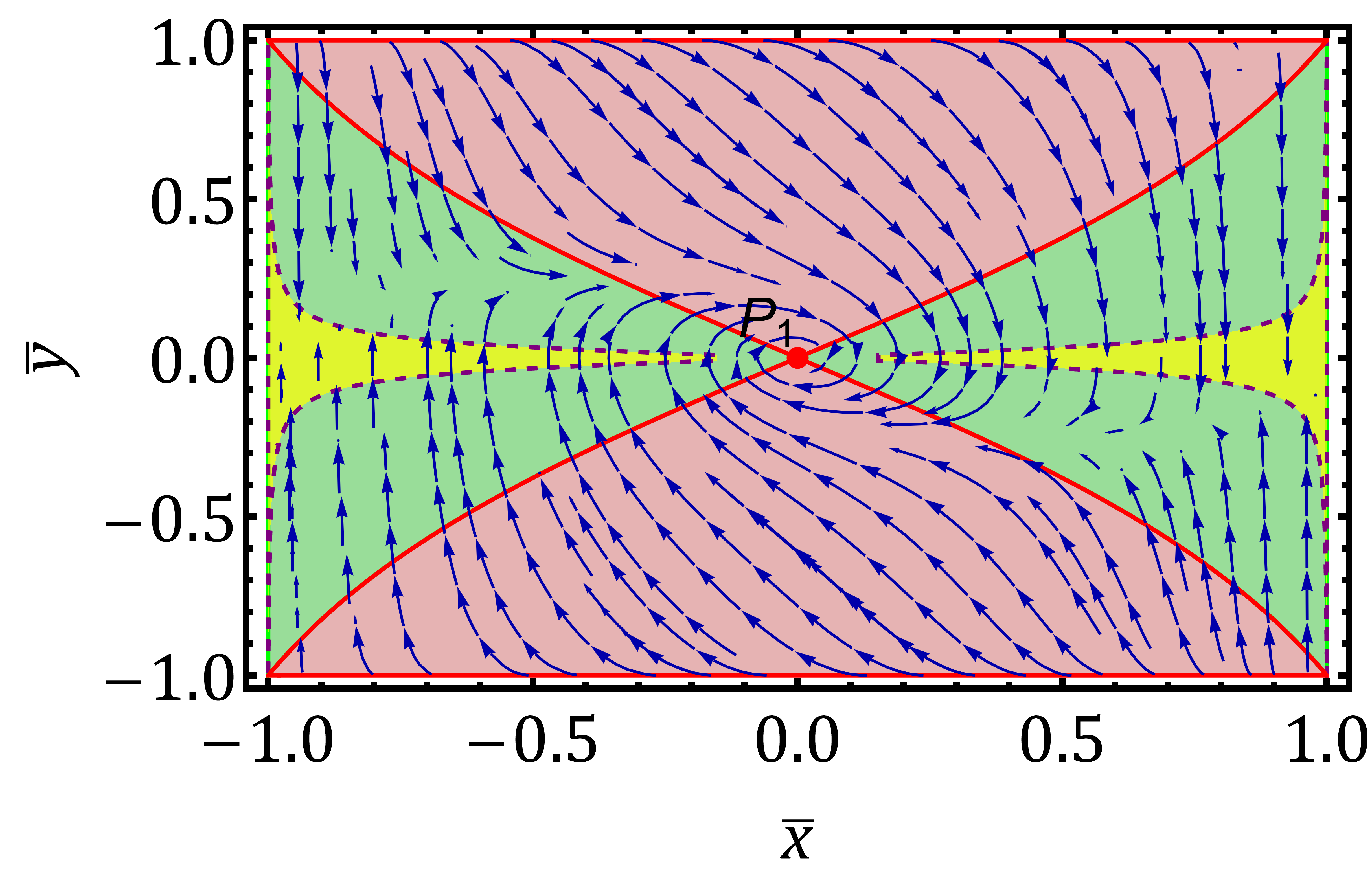
Figure 1: The phase space of inflaton field in the variable $(\bar{x},\bar{y})$, where yellow region represents $0<\epsilon_{1}<0.1$, green region shows $0.1<\epsilon_{1}<1$ and pink region signifies $\epsilon_{1}>1$, and .

The Klein-Gordon equation (Eq. (2.5)) and the second Friedmann equation (Eq. (2.7)) can be recast in terms of the dynamical variables $\bar{x}$ and $\bar{y}$ which constitute the autonomous equations of this system:

$$\bar{x}^{\prime} = \frac{\bar{y}\left(1-\bar{x}^{2}\right)^{3/2}}{\sqrt{1-\bar{y}^{2}}}\,,$$ (2.21)

$$\bar{y}^{\prime} = \frac{3\bar{y}\sqrt{1-\bar{y}^{2}\bar{x}^{2}}\sqrt{\left(1-2\bar{y}^{2}\right)\bar{x}^{2}+\bar{y}^{2}}}{\left(1-\bar{y}^{2}\right)^{3/2}\left(\bar{x}^{2}-1\right)}-\frac{\bar{x}}{\sqrt{1-\bar{x}^{2}}}\ ,$$ (2.22)

where the prime denotes derivatives with respect to the dimensionless time $t^{\prime}=mt$. It is to note that now the dynamical equations are written in the form given in Eqs. (2.3) and have no further pathologies. It is then straightforward to write down the Jacobian as in Eq. (2.4) and find the fixed points. The analysis yields a single critical point at $P_{1}=(0,0)$, where both $\bar{x}$ and $\bar{y}$ vanish. At $P_{1}$ both $\phi$ and $\dot{\phi}$ vanishes and consequently the Hubble parameter is also zero. It turns out to be a stable fixed point. It must be stated here that $P_{1}$ is the only fixed point in this case, and there are no fixed points at infinity as in the compact phase space the points at infinity have been mapped to the borders $\bar{x}=\pm 1$ and $\bar{y}=\pm 1$. Any possible critical points at infinity would have appeared as critical points on those lines. Fig. [1] illustrates the phase-space trajectories, with color-coded regions: the yellow and green regions correspond to spaces where $0<\epsilon_{1}<0.1$ and $0.1<\epsilon_{1}<1$ and hence these regions are the slow-roll regions, whereas the pink region corresponds to portions of the phase space where $\epsilon_{1}>1$. On the boundary curve between the pink region and the green region (bordered in red) we have $\epsilon_{1}=1$.

As far as cold inflation is concerned, we know that in such inflationary cases the slow-roll parameter starts with a value much less than unity and inflation goes on until $\epsilon_{1}\sim 1$. Consequently in the phase space of the system inflationary trajectories are those which start in the yellow region and continuously travels towards the pink region through the green region. We can spot such inflationary trajectories both on the left and right sides of the fixed point $P_{1}$ in Fig. [1]. Here we must remind the reader that some of these trajectories may seem to again enter a inflationary phase as shown in the phase space plot. Does the phase space imply multiple inflationary phases? The answer is no. The reason being the plot in Fig. [1] is purely a dynamical systems analysis of the cold inflationary model and does not contain any information about reheating and graceful exit. In reality as soon as one of the trajectories starts from the yellow region and nears the pink region the physics of the system changes as graceful exit takes place. The phase space plot only gives us the information about those trajectories that may produce inflation.

The phase space picture shows that most of the trajectories, corresponding to various kinds of initial conditions, ends up in an inflationary phase. In this sense cold inflation is an attractor solution. Although we have shown the attractor like solution with respect to a particular inflaton potential, for any other potential which allows inflation will have a similar kind of phase space structure.

3 Dynamical analysis of cold inflation in the constant-roll regime

Constant-roll cold inflation (CRCI) was first introduced in [83, 84], and the theory of CRCI was subsequently expanded and developed in [62, 64, 65, 63]. Some of these papers have also carried out a dynamical system analysis of the inflationary process in constant-roll regime [66, 64]. However, these previous studies were not solely dedicated to fully analyze the attractor nature of CRCI in a detailed manner. Here, we develop the general techniques and explore the dynamical system of CRCI. In CRCI all the essential dynamical equations of cold inflation, as discussed in the previous subsection, are valid in addition with an extra constant-roll condition given by:

$$\ddot{\phi}=-3\beta H\dot{\phi}\,,$$ (3.1)

where $\beta$ is a parameter that generalizes both slow-roll and ultra-slow-roll inflation. This framework generalizes inflationary dynamics, as demonstrated in Eq. (7) of Ref. [84] where the parameter $\beta$ is related to $\alpha$ by the expression:

$$\beta=\frac{1}{3}(\alpha+3)\ .$$ (3.2)

The condition in Eq. (3.1) modifies the cold inflation dynamics radically. For instance, as $\beta\to 0$, the model approaches the slow-roll (SR) limit, whereas $\beta\to 1$ corresponds to the ultra-slow-roll (USR) limit. This indicates that the larger the value of $\beta$, the more is the departure from the standard slow-roll dynamics. Moreover, unlike slow-roll cold inflation where one is free to choose the inflationary potential, the form of the potential during CRCI gets fixed by the constant-roll dynamics. Depending on whether $\beta$ is positive or negative, different forms of potentials can be derived that are suitable for CRCI dynamics. Above all, the graceful exit condition from a constant-roll dynamics can be different in cases with $\beta$ positive or negative as was first pointed out in Ref. [79].

Here, we will represent dynamical analysis of CRCI using stream-plots as usage of autonomous equations turns out to be a difficult issue because of the constant-roll condition. The stream-plots will show the dynamical trajectories of the system and are capable of showing the attractor nature of the inflationary solution.
In the present section we will discuss:

1. the stability issue of CRCI dynamics for positive and negative values of $\beta$.

2. The issue related to graceful exit in CRCI.

3. How does the attractor nature of CRCI differ from pure CI?

In Ref. [79] the authors pointed out about the graceful exit problem in CRCI for both positive and negative values of $\beta$. In this article we verify the claims made in the reference. We show that in CRCI the attractor nature of inflation changes from cold inflation.

3.1 Case I: $\mathbf{\beta>0}$

First we focus on the model for positive $\beta$, i.e., $\alpha>-3$. The corresponding potential for CRCI is given by [84]

$$V(\phi)=V_{0}\left[\left(1-\beta\right)\cosh^{2}\left(3\kappa\sqrt{\frac{\beta}{6}}(\phi_{0}-\phi)\right)-1\right].$$ (3.3)

Here $V_{0}\equiv 3M^{2}M^{2}_{\rm Pl}$ is a positive constant, $M$ is a constant with the dimension of mass and $\phi_{0}$ is a constant value of the inflaton field at some fixed time. In Ref. [84], H. Motohashi et al. claimed that for a potential given in their Eq. (2.26)– which corresponds to Eq. (3.3) in the present work– the Hubble parameter in the context of CRCI is expressed as $H=M\tan[-3\beta Mt]$. However, this expression is incomplete. The correct and complete form of the Hubble parameter is:

$$H=M\tan(-3\beta Mt+C)\,,$$ (3.4)

where $C$ is an integration constant. Assuming $M>0$, the Hubble parameter remains positive when the following condition is satisfied:

$$0\leq-3\beta Mt+C<\frac{\pi}{2}\,.$$ (3.5)

By restricting the argument of the tangent function to the first quadrant, the inequality becomes:

$$\frac{1}{3\beta M}\left(C-\frac{\pi}{2}\right)<t\leq\frac{C}{3\beta M}\,,$$ (3.6)

which can always be fulfilled if $C\sim\pi/2$ and adjusting the value of $M$. This condition specifies $H>0$. As the scale-factor $a$ is always assumed to be greater than zero, implies $\dot{a}>0$. The authors of the above mentioned paper opines (after Eq. (2.29) of their work) that “Although this is a mathematically allowed solution, it has $\ddot{a}(t)<0$. Therefore, it cannot describe an inflationary model in the usual sense.” We show that such a conclusion is erroneous, there exists initial conditions and parameter values for which both $\dot{a}>0,\ \ \ddot{a}>0$.
We have

$$H\equiv\frac{\dot{a}}{a}=M\tan(-3\beta Mt+C)\,,$$ (3.7)

which gives $\dot{a}=M\tan(-3\beta Mt+C)a$ and consequently:

$$\ddot{a}=-aM^{2}[3\beta+(3\beta-1)\tan^{2}(-3\beta Mt+C)]\,.$$ (3.8)

In the limit $3\beta\to 0$, we see that the above expression can indeed produce $\ddot{a}>0$ during some inflationary epoch. Only when $3\beta>1$ we do not find any possibility of inflation.

To analyze the dynamics associated with the potential given in Eq. (LABEL:cr_v_betac_positive), we begin with the equation of motion for the inflaton field $\phi$ as given in Eq. (2.5). Substituting the constant-roll condition from Eq. (3.1), the modified equation of motion for the inflaton field becomes:

$$3(1-\beta)H\dot{\phi}+V_{,\phi}=0.$$ (3.9)

It is important to note that the primary distinction between slow-roll and constant-roll inflation lies in the equation of motion for the inflaton field and the form of the potential. The remaining equations, specifically the first and second Friedmann equations, remain unchanged.

To understand the dynamics in this scenario, we define the dynamical variables as follows:

$$x=\pm\frac{\sqrt{V}}{\sqrt{3V_{0}}},\quad y=\frac{\dot{\phi}}{\sqrt{6}\sqrt{V_{0}}},\quad z=\frac{H}{\kappa\sqrt{V_{0}}}.$$ (3.10)

These dynamical variables are structurally similar to those defined for the earlier case and yield the same value of the slow-roll parameter used in the earlier case: $\epsilon_{1}=3y^{2}/(x^{2}+y^{2})$. Due to the different constants involved in the potential, we normalize the field and the Hubble parameter with the constant $V_{0}$, thereby constructing dimensionless dynamical variables. One must note that in the present case the potential in Eq. (LABEL:cr_v_betac_positive) is not positive definite. This potential may admit negative values for some parameter choice and some values of the initial conditions. As because negative value of the scalar field potential can never produce inflation, we have worked with those initial conditions for which $V(\phi)$ is non-negative and consequently $x$ is properly defined everywhere in the phase space. From the form of the potential it is evident that when $\phi\sim\phi_{0}$, $V(\phi)$ turns negative and consequently in the present case we only analyze those dynamical regions where $x>0$ or $x<0$ as $x$ never crosses zero.

It is worth noting that, in this case, the constant-roll inflation condition reduces the second-order differential equation for $\phi$ to a first-order equation. Hence, we can express the field $\phi$ in terms of the dynamical variable using Eqs. (3.3) and (3.10):

$$\kappa\phi=\kappa\phi_{0}-\frac{1}{3}\sqrt{\frac{6}{\beta}}\ \cosh^{-1}\left(\sqrt{\dfrac{3x^{2}+1}{1-\beta}}\right)\ .$$ (3.11)

The above equation show that in our whole analysis $\beta<1$. The potential we are working with turns out to be purely negative for $\beta>1$ and consequently never produces inflation like solutions as in this regime $\ddot{a}<0$. Using the derivative of the potential:

$$V_{,\phi}=-3\kappa V_{0}(1-\beta)\sqrt{\frac{\beta}{6}}\sqrt{\left(\frac{2(3x^{2}+1)}{1-\beta}-1\right)^{2}-1}\,,$$ (3.12)

the variable corresponding to $\dot{\phi}$ can be expressed using Eq. (3.9):

$$y=\pm\frac{\sqrt{\beta}}{6z}\sqrt{\left(\frac{2(3x^{2}+1)}{1-\beta}-1\right)^{2}-1}\ .$$ (3.13)

The variable $y$ is expressed in terms of $z$ and $x$ via the Hubble constraint relation:

$$z^{2}=x^{2}+y^{2}\,,$$ (3.14)

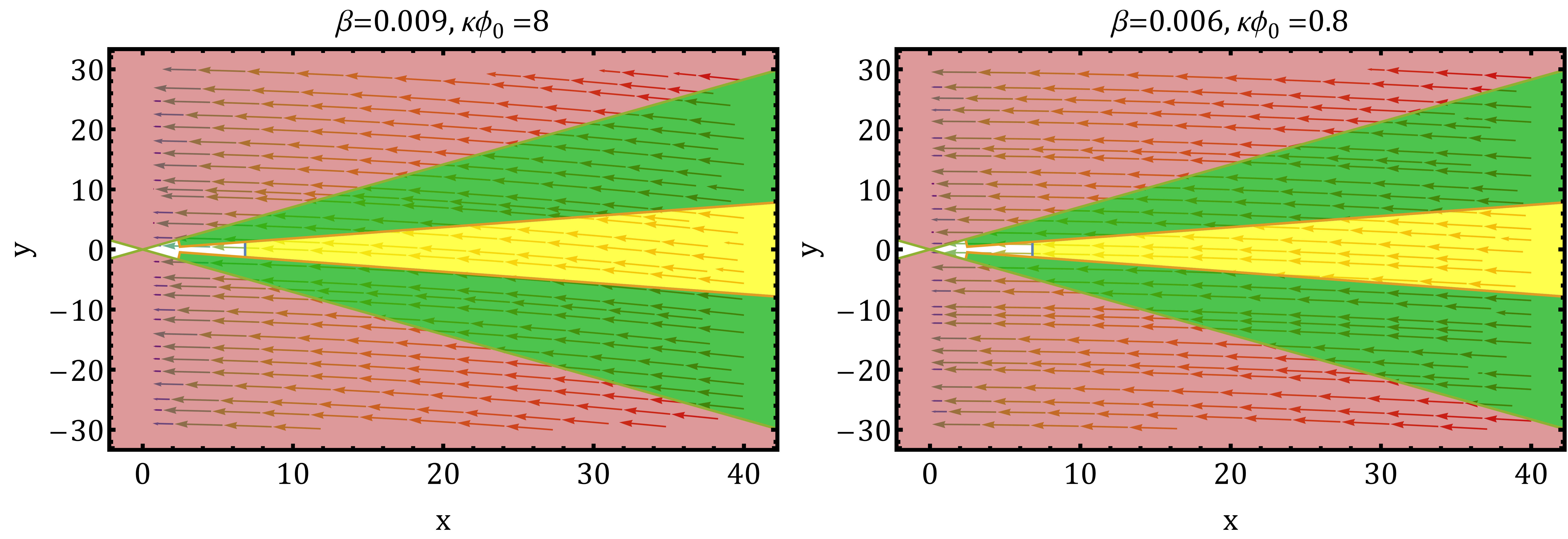
Figure 2: The streamline plots for the field $(\kappa\phi,\dot{\phi}/\sqrt{V_{0}})$ in a specific $(x,y)$ range. The curves correspond to streamlines for different values of $\beta>0$ and field constants. The color code is as follows: the green region represents regions where $0<\epsilon_{1}<1$, in the pink region $\epsilon_{1}>1$ and in the yellow region we have $0<\epsilon_{1}<0.05$.

which gives $z$ in terms of $x$ and $y$. We have produced the streamline plots for the field $(\dot{\phi}/\sqrt{V_{0}},\kappa\phi)$ in some specific range of $x$ and $y$. The stream lines are the flow lines for the vector field $(\kappa\phi,\dot{\phi}/\sqrt{V_{0}})$. The stream-plots are shown in Fig. [2] for different values of $\beta$ and $\kappa\phi_{0}$. Each stream-plot is divided into distinct colored regions: the green region represents $0<\epsilon_{1}<1$, the pink region represents $\epsilon_{1}>1$, and the yellow region represents $0<\epsilon_{1}<0.05$. On the boundary curve, differentiating the green and the pink regions, $\epsilon_{1}=1$.

The flow-line plots are done for $x>0$, and the flow lines are towards the minimum of the potential (towards $x=0$). When $\beta$ is reasonably small (near the slow-roll limit), for both the two plots in Fig. [2], it is seen that the streamlines originating in the yellow region, with negative as well as positive values of $\dot{\phi}$ in the right side of the plots, have initial value of $\epsilon_{1}$ to be very small. Most of these flow lines leave the yellow region and move towards the pink region through the green patch. These flows represent potential inflationary flows. As soon these lines come near the pink region, inflation ends. It is seen that near the slow-roll limit, CRCI still remains an attractor solution. In the present case we do not employ the autonomous equations to figure out the inflationary dynamics as there is only one independent variable and the phase space is one dimensional. The streamline plots in the present case do not give us any information about the fixed points in CRCI.

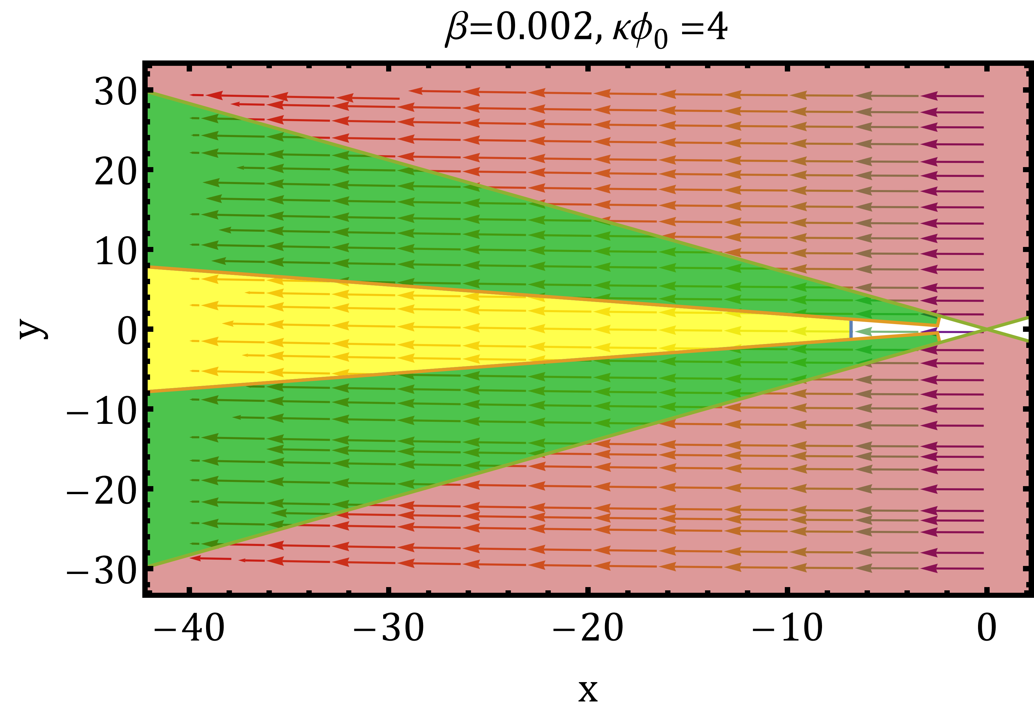
Figure 3: The streamline plots for the field $(\kappa\phi,\dot{\phi}/\sqrt{V_{0}})$ in a specific $(x,y)$ range. Streamlines for $\beta=0.002$, illustrating that they remain confined within the inflation region and do not exit. The color coding is the same as the previous figures.

For a complete description of CRCI dynamics one should note that in this case one encounters eternally inflating trajectories in the stream-plots for appropriate parameters and range of the variables. In Fig. [3], we plot the stream lines for negative values of $x$. In this case one is moving away from $V(\phi)=0$. The plot shows that there are stream lines which will eternally be inside the yellow region, if initially they start from the yellow region. For these kind of dynamics the stream lines never get a chance to reach the pink region. This is a generic feature of most CRCI models.

In the present case the standard autonomous system of equations are not required as the system is solvable algebraically and the flow dynamics specified by $(\kappa\phi,\dot{\phi}/\sqrt{V_{0}})$, as shown in Fig. [2], is sufficient in the present case and shows the qualitative behavior of the system exhaustively.

3.2 Case II: $\mathbf{\beta<0}$

In this section, we will be investigating the scenario where the constant roll parameter $\beta$ can take negative values. Hence, the corresponding constraint equation becomes:

$$\ddot{\phi}=3\tilde{\beta}H\dot{\phi}\ ,$$ (3.15)

where we redefined $\beta$ as $\tilde{\beta}=-\beta$. It has been shown in Ref. [84] that negative $\beta$ modifies the form of the potential. Therefore, the corresponding potential as mentioned in Ref. [84] is

$$V(\phi)=V_{0}\left[1-(1+\tilde{\beta})\sin^{2}\left(3\kappa\sqrt{\frac{\tilde{\beta}}{6}}(\phi+\phi_{0})\right)\right]\ .$$ (3.16)

As we introduce the redefined constant roll parameter $\tilde{\beta}$, the corresponding equation of motion of the inflaton field, assuming the constant-roll constraint, becomes:

$$3H\dot{\phi}(1+\tilde{\beta})+V_{,\phi}=0\ .$$ (3.17)

To proceed with the dynamical analysis of the system, as carried out in the previous case, we use similar dimensionless variables as defined in Eq. (3.10), as both cases have a similar structure. In the present case also the potential $V(\phi)$ admits negative values and consequently we have to work either with positive values or negative values of $x$. As inflation always occurs when $V(\phi)>0$ we do not work with those initial conditions which produce negative scalar field potential.

Due to the definition of the variables, the field $\phi$ can be expressed as:

$$\kappa\phi=\frac{1}{3}\sqrt{\frac{6}{\tilde{\beta}}}\sin^{-1}{\left(\sqrt{\frac{1-3x^{2}}{1+\tilde{\beta}}}\right)}-\kappa\phi_{0}\ .$$ (3.18)

Similarly, the gradient of the potential becomes:

$$V_{,\phi}=\pm 3\kappa V_{0}(1+\tilde{\beta})\sqrt{\frac{\tilde{\beta}}{6}}\sqrt{1-\left(\dfrac{2(1-3x^{2})}{(1+\tilde{\beta})}-1\right)^{2}},$$ (3.19)

and the time derivative of the field $(\dot{\phi}\propto y)$ can be expressed as:

$$y=\pm\frac{\sqrt{\beta}}{6z}\sqrt{1-\left(\dfrac{2(1-3x^{2})}{(1+\tilde{\beta})}-1\right)^{2}}\ .$$ (3.20)

It is important to note that from Eq. (3.18), the argument of the inverse sin function must lie within the range $[-1,1]$. This imposes the constraint on $x$:

$$-\frac{1}{\sqrt{3}}<x<\frac{1}{\sqrt{3}}\,.$$

The above condition shows one of the differences of CRCI, with negative $\beta$, with respect to the case of positive $\beta$. In the present case the range of $x$ is bounded. This also puts a bound on the maximum value of $y$, for $\tilde{\beta}=0.0067$. The bounded interval for $y$ is $(-0.4,0.4)$.

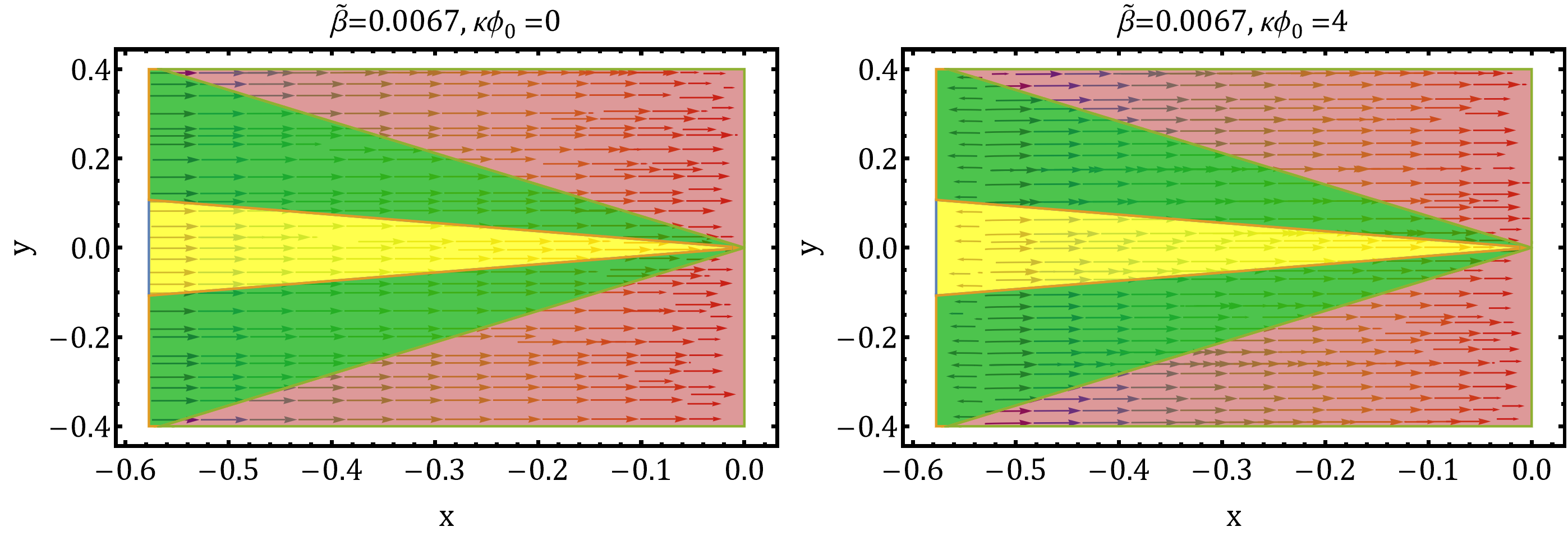
Figure 4: The streamline plots for the field $(\kappa\phi,\dot{\phi}/\sqrt{V_{0}})$ in a specific $(x,y)$ range. The curves correspond to streamlines for $\beta<0$. For these plots $\tilde{\beta}=0.0067$ and the field constant vary. Here green region corresponds to regions where $0.1<\epsilon_{1}<1$, pink region corresponds $\epsilon_{1}>1$, and yellow region corresponds to $0<\epsilon_{1}<0.1$.

As in the case of positive $\beta$, we have constructed the stream-plots showing the nature of streamlines corresponding to the components $(\kappa\phi,\dot{\phi}/\sqrt{V_{0}})$ by varying the independent variable $x$. The streamline plots are shown in Fig. [4]. For this analysis, we have chosen $\tilde{\beta}=0.0067$, as this value corresponds to a spectral index $n_{s}=0.96$, consistent with the value obtained in [84].

In the case of negative $\beta$, the stream-plots exhibit a similar attractor like solution as in the previous case, however this time we have only confined the dynamics only in the negative $x$ region. The stream lines plotted in Fig. [4] compel the system to move towards potential zero. It is seen in this case that all the streamlines originating on the left most side must be streaming in such a way that for all of them $\dot{\epsilon_{1}}>0$. This behavior aligns with the findings of Ref. [79].

Like the previous case for $\beta>0$, in this case also we get the phase space behavior algebraically. It is important to note that the extra constant-roll condition permits the existence of inflationary phase in both the cases discussed in this section, for positive and negative values of $\beta$. In both the cases it is observed that the attractor nature of inflation has been affected by the constant-roll condition. When we compare our results with the result of cold inflation (as given in the previous section) we see that only a part of the phase space trajectories end up in inflationary phase in the present case whereas in the case of cold inflation mostly all trajectories were attracted towards some inflationary phase.

Before we finish our discussion on CRCI it is important to specify that the authors in Ref. [66, 85] have studied the large $\beta$ behavior of CRCI models and have shown that these models do not in general show attractor behavior. They conclude that only small $\beta$ solutions, which specify slow-roll limit of CRCI, can only produce attractor like solutions. In the present paper we have not delved into the large $\beta$ limit as our primary aim was to unravel the attractor nature of CRCI.

4 Warm Inflation (WI)

The warm inflation scenario arises when the inflaton field dissipates energy into lighter degrees of freedom at a rate exceeding the Hubble expansion rate. This dissipation mechanism ensures that the generated particles thermalize efficiently, creating a radiation bath. During this epoch, these light particles can be modeled as radiation, with the radiation energy density given by:

$$\rho_{r}=\frac{\pi^{2}g_{*}T^{4}}{30},$$ (4.1)

where $\rho_{r}$ is the radiation energy density, $g_{*}$ is the effective number of relativistic degrees of freedom, and $T$ is the temperature of the generated particles.

The evolution of the inflaton field $\phi$ and the radiation energy density $\rho_{r}$ in a spatially flat FLRW background is described by the following equations:

$$\ddot{\phi}+3H\dot{\phi}+V_{,\phi} = -\Upsilon(\phi,T)\dot{\phi}\ ,$$ (4.2)

$$\dot{\rho}_{r}+4H\rho_{r} = \Upsilon(\phi,T)\dot{\phi}^{2}\ .$$ (4.3)

Here $\Upsilon$ is the dissipation rate, the rate at which the inflaton sector dissipates energy to the radiation bath. One can get a form of $\Upsilon$ from the microphysics of the system. The form of $\Upsilon$ depends upon the nature of particles produced via the decay of the inflaton. If these decays (to multiple types of particles) happen near a thermal equilibrium one may expect $\Upsilon$ to be a function of the ambient temperature of the radiation bath and the inflaton field strength. As $\Upsilon$ is related to the decay rate of the inflaton, we must obviously have the following dynamical constraint:

$$\Upsilon\geq 0\,.$$ (4.4)

When $\Upsilon=0$, the radiation and the scalar field sector decouples. In general the dissipative factor can be expressed as [37, 39, 38, 40]:

$$\Upsilon=C_{1}T^{c}\phi^{p}M^{1-p-c}\ ,$$ (4.5)

where $C_{\Upsilon}$ is a dimensionless constant, $c,p$ are the free parameters of the model and $M$ is the mass dimensional constant. In the literature the following forms of the $\Upsilon$ have been studied extensively [37, 39, 38, 40].

$$\rm(i)\ T\quad(ii)\ T^{3}\quad(iii)\ \frac{T^{3}}{\phi^{2}}\ .$$ (4.6)

The energy density and the pressure of the inflaton field are:

$$\rho_{\phi}=\frac{1}{2}\dot{\phi}^{2}+V(\phi),\quad P_{\phi}=\frac{1}{2}\dot{\phi}^{2}-V(\phi)\ .$$ (4.7)

The first and second Friedmann equations are:

$$3H^{2} = \kappa^{2}(\rho_{r}+\rho_{\phi})\ ,$$ (4.8)

$$2\dot{H} = -\kappa^{2}\left(\dot{\phi}^{2}+\frac{4}{3}\rho_{r}\right)\ .$$ (4.9)

Given a form of $\Upsilon$ one can see whether one can get a state of inflation, during which the slow-roll conditions are maintained. During such a slow-roll phase the radiation bath maintains a dynamic equilibrium so that one can attach a temperature $T$ of the radiation bath. Warm inflation happens as long as $T>H$. To ensure that the warm inflation field can initiate the consistent inflationary epochs, a number of slow roll parameters are usually defined as:

$$\epsilon_{1}=-\frac{\dot{H}}{H^{2}},\quad\eta_{1}=\dfrac{1}{\kappa^{2}(1+Q)}\dfrac{V_{,\phi\phi}}{V},\quad\beta=\dfrac{\Upsilon_{,\phi}V_{,\phi}}{\kappa^{2}V\Upsilon}\,.$$ (4.10)

Additionally, in this case we do not assume that the radiation bath has a fixed temperature initially. However, it may happen the system ultimately settles down to a phase where $\rho_{r}$ becomes a constant, with $T>H$, and we may interpret the dynamics of that phase to be the dynamics of a warm inflationary phase, if the slow-roll conditions are satisfied. If cosmological dynamics does not produce a phase with nearly a constant radiation energy density then we do not get a proper warm inflationary phase. Moreover, throughout the dynamical evolution of the system, the radiation energy density must be positive i.e. $\rho_{r}>0$ and the system must be thermally stable:

$$\frac{|\dot{\rho}_{r}|}{H\rho_{r}}\ll 1\ ,\quad\text{or equivalently}\quad\frac{|\dot{T}|}{HT}\ll 1.$$ (4.11)

In the subsequent section, we will explore the phase space dynamics corresponding to the quadratic potential of the inflaton field, which takes the following form:

$$V(\phi)=\frac{1}{2}m^{2}\phi^{2}\,,$$

where $m$ represents the mass of the inflaton field. This potential form remains the same as the form of the potential used in cold inflation.

4.1 Dynamics of the Warm Inflation field

To analyze the dynamics of the inflaton field for various classes of dissipative models described in Eq. (4.6), we define a set of dimensionless dynamical variables to effectively capture the phase space dynamics:

$$x=\frac{\kappa\sqrt{V}}{\sqrt{3}H},\quad y=\frac{\kappa\dot{\phi}}{\sqrt{6}H},\quad\Omega_{r}=\frac{\kappa^{2}\rho_{r}}{3H^{2}},\quad z=\frac{H}{m},\quad Q=\frac{\Upsilon}{3H}\ .$$ (4.12)

Here, the variables $x$ and $y$ correspond to the field potential and the field’s velocity, respectively, normalized by the Hubble parameter. Additionally, the variable $z$ represents the Hubble parameter $H$, which is introduced to close the system of equations. As we will move over to CRWI in the next section, where we will be only treating cases where $Q$ is a constant or it is a function of temperature, we will like to analyze these two cases in this section so that we can have some comparison of the results. As because we assume thermal stability, we do not separately give detailed analysis about $Q$ depending purely on $T$ as when $T$ is nearly a constant (for thermal stability) $Q$ is also a constant. Consequently, the case of constant $Q$ encompasses both results approximately. Henceforth we present the dynamical analysis assuming a constant $Q$.

The authors in Ref. [53] had initiated a detailed study of the dynamical system related to warm inflation. In the present paper we use the same form of inflaton potential in warm inflation. In this reference the authors worked with a case where $\Upsilon$ was independent of temperature and so was $Q$. In such a case authors did not explicitly use the thermalization constraint and moreover the authors did not construct compactified phase space. As a result of these the authors had to specifically carry out an investigation to figure out the asymptotic solutions. It is assumed that the authors did not test whether $|\dot{T}|/HT<1$ because they were tacitly relying on slow-roll warm inflation where time rate of changes of physical quantities happens slowly. In our case we work with a set of initial conditions and see how the phase space trajectories evolve. We see that there can be trajectories which do not obey the thermal stability criterion (and hence slow-roll criterion) but are dynamically possible. Moreover our phase space dynamics also shows that the slow-roll region does not coincide with the thermally stable region or in other words we can have regions in phase space where $\epsilon_{1}<1$ but $|\dot{T}|/HT>1$.

In Ref. [54] the authors have studied the stability of warm inflationary models which are evolving near the slow-roll limit. They have worked out the conditions of stability of the system near slow-roll evolution. In our work we have focused our attention on the entire available phase space of the system and all possible trajectories. Out of these possible phase space trajectories some correspond to slow-roll evolution. Our work is more focused on the generic phase space morphology of warm inflation and the presentation of the warm inflation dynamics, provided in this section, gives a new way of dealing with warm inflationary stability issues as will become clearer as one goes through the details of the subject presented.

4.1.1 The case where  Q = Constant

The Hubble constraint equation, expressed in terms of the dynamical variables, takes the form:

$$1=\Omega_{r}+x^{2}+y^{2}\ ,$$ (4.13)

and the Raychaudhuri equation, in terms of the dynamical variables, is expressed as:

$$\frac{\dot{H}}{H^{2}}=-3\left(y^{2}+\frac{2}{3}\Omega_{r}\right)\,.$$ (4.14)

The other constraints, particularly the thermal stability condition, can be expressed in terms of the dynamical variables as:

$$0\leq\Omega_{r}\leq 1,\quad\frac{|\dot{\rho}_{r}|}{H\rho_{r}}=\left|\frac{6Qy^{2}}{\Omega_{r}}-4\right|\ll 1\,.$$ (4.15)

The slow-roll parameter, in the present case, becomes

$$\epsilon_{1}=3\left(y^{2}+\frac{2}{3}\Omega_{r}\right)\ .$$ (4.16)

The autonomous equations corresponding to $(x,y,z)$ can be expressed in terms of the dynamical variables as:

$$x^{\prime} = \frac{y}{z}-x\frac{\dot{H}}{H^{2}}\ ,$$ (4.17)

$$y^{\prime} = -3y(1+Q)-\frac{x}{z}-y\frac{\dot{H}}{H^{2}}\ ,$$ (4.18)

$$z^{\prime} = z\frac{\dot{H}}{H^{2}}\ .$$ (4.19)

Here, $()^{\prime}\equiv d()/dN$, where $N$ is the number of $e$-folds. As the autonomous system of equations requires three independent variables to close the system, the phase space becomes 3-dimensional. From the above equations, it can be observed that the variable $z$ presents an invariant sub-manifold at $z=0$, although the system of equations becomes ill defined near $z=0$. We will tackle the singularity of the system of equations at $z=0$ shortly. According to the definition of $z$ in Eq. (4.12), the value of $z$ is positive. Hence, the region of interest in the phase space is the positive $z$-axis.

Before analyzing the qualitative behavior of the system, let us discuss the range of the dynamical variables to examine the compactness of the phase space. From the Friedmann constraint relation Eq. (4.13), the ranges of the variables $(x,y)$ are:

$$-1\leq x\leq 1,\quad-1\leq y\leq 1\ .$$ (4.20)

Meanwhile, the range of the variable $z\in[0,\infty)$ makes the phase space non-compact. The value of $z$ near zero implies the value of $H$ is infinitesimally small or $H\ll m$.

To compactify the phase space, we transform the variable $z$ to $\bar{z}$ using the Poincaré transformation:

$$\bar{z}=\frac{z}{\sqrt{1+z^{2}}}\ ,$$ (4.21)

mapping infinities to a finite range, $\bar{z}\in[0,1)$, transforming the phase space into a cylindrical geometry with unit radius. With this compactification, the new autonomous system of equations becomes:

$$x^{\prime} = \frac{y}{\bar{z}}\sqrt{1-\bar{z}^{2}}-x\frac{\dot{H}}{H^{2}}\ ,$$ (4.22)

$$y^{\prime} = -3y(1+Q)-\frac{x}{\bar{z}}\sqrt{1-\bar{z}^{2}}-y\frac{\dot{H}}{H^{2}}\ ,$$ (4.23)

$$\bar{z}^{\prime} = (1-\bar{z}^{2})\bar{z}\frac{\dot{H}}{H^{2}}.$$ (4.24)

Here, the prime denotes the derivative with respect to the number of $e$-folds, and $\bar{z}$ represents an invariant submanifold at $\bar{z}=0$. However, it must be noted that the autonomous equations diverge as $\bar{z}\to 0$, making this a pathological coordinate. To eliminate this divergence while preserving the qualitative analysis of the system, we adopt a standard procedure commonly used in the dynamical analysis of systems, as discussed in section 2. This method is used in Ref. [15]. The redefined $e$-fold number then becomes:

$$dN\mapsto\bar{z}^{n}\ dN^{\prime}.$$ (4.25)

The redefinition ensures that the system remains finite at $\bar{z}=0$, validating the system around this critical point. It is important to note that the values of $n$ are model-dependent and must be chosen carefully. These values are determined by analyzing the order of divergence in the dynamical equations. For instance, if the system contains a term of the form $1/\bar{z}^{2}$, the time redefinition should be $dN\mapsto\bar{z}^{2}dN$. Crucially, the redefinition must not exceed the actual order of divergence; overcompensating can inadvertently introduce spurious fixed points and distort the true phase space structure of the system. Additionally, if the expression contains multiple pathological terms—as will be encountered in the subsequent section—these divergences must be addressed collectively, with careful attention paid to the respective orders of divergence to ensure consistent and accurate regularization. Interested readers may refer to Ref. [16] to gain in-depth insight on this technique. In the present case, $n=1$, and Eqs. (4.22)–(4.24) become after redefinition of $N$:

$$x^{\prime} = y\sqrt{1-\bar{z}^{2}}-x\bar{z}\frac{\dot{H}}{H^{2}}\ ,$$ (4.26)

$$y^{\prime} = -3y\bar{z}(1+Q)-x\sqrt{1-\bar{z}^{2}}-y\bar{z}\frac{\dot{H}}{H^{2}}\ ,$$ (4.27)

$$\bar{z}^{\prime} = (1-\bar{z}^{2})\bar{z}^{2}\frac{\dot{H}}{H^{2}}.$$ (4.28)

Fixed points for constant $Q$
Points	$(x_{*},y_{*},\bar{z}_{*})$	$\Omega_{\phi}$	$\epsilon_{1}$	$\frac{\dot{\rho}_{r}}{H\rho_{r}}$	Stability
$P_{1}$	$(0,0,0)$	$0$	$\sim 2$	$\sim-4$	Stable
$P_{2,3}$	$(\mp 1,0,1)$	$1$	0	Indeterminate	Saddle
$P_{4}$	$(0,0,1)$	$0$	$2$	$-4$	Unstable
$P_{5}$	$(0,\sqrt{1+3Q},1)$	$1+3Q$	$3(1+Q)$	$-6(1+Q)$	Saddle

Table 1: The critical points and their nature for WI for constant $Q$.

In all the above equations one has to replace the value of ${\dot{H}}/{H^{2}}$ by the expression of it, given in Eq. (4.14).

Next, we will determine the qualitative behavior of the system by identifying the critical points corresponding to the model. The critical points and their nature for the model are summarized in Tab. [1]. In the table, we have included the stability of the system at these fixed points. The stability is determined by the methods explained initially in section 2 of this article. In the present case we have a constant dissipative factor $Q$. This dynamical system exhibits five critical points, as shown in Tab. [1], where only one fixed point, labeled as $P_{5}$, is $Q$-dependent. At this point, the field fractional energy density is also $Q$-dependent, given by $\Omega_{\phi}=1+3Q$. For any non-zero positive value of $Q$, $\Omega_{\phi}$ exceeds 1, which implies a negative radiation energy density ($\Omega_{r}<0$), rendering this point invalid. Consequently, $P_{5}$ is not considered in the phase space analysis. On the other hand, the remaining fixed points are independent of $Q$.

At point $P_{1}$, all coordinates vanish. This fixed point is unusual, as one will not be able to properly calculate the field energy density or radiation energy density as because the definition of $x,y,\Omega_{r}$ contains division by factors of $H$. As at this point, $z=0$, we have $H=0$. We have shown this fixed point in the plots as because many phase space trajectories travel towards this point. Heuristically, this point represents the far future of the universe when the Hubble parameter tends to zero. This point appears to be a stable fixed point. Near about this point the slow-roll parameter is greater than one showing that this region is not in the inflationary phase and moreover there can be large fluctuations of radiation energy density near about this point.

Points $P_{2}$ and $P_{3}$ represent field-dominated states with a sub-dominant kinetic component ($|y|\ll x$). These points occur in the potential energy dominated phase. In these cases, the slow-roll parameter becomes much smaller than 1, indicating that phase trajectories may come nar to these point during the early inflationary period. However, the thermal condition $\dot{\rho}_{r}/(H\rho_{r})$ cannot be uniquely determined around these points. The system exhibits saddle behavior at these points, characterizing an early accelerating phase.

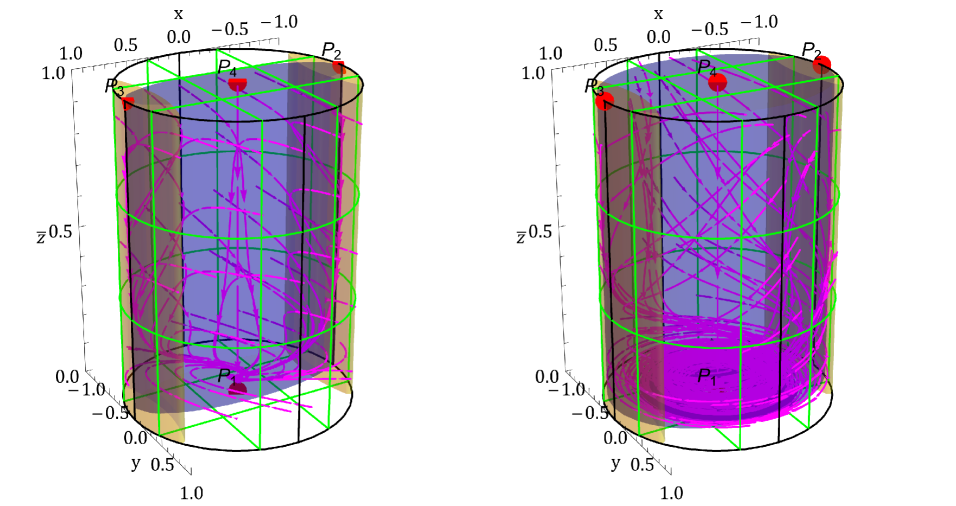
Figure 5: The phase space dynamics corresponding to $Q=5,\ 0.5$, displayed in the left and right hand side plots.

Point $P_{4}$ shows unstable behavior and around this point the universe is primarily radiation dominated, scalar field energy density is zero around this point. For the purpose of inflation, this point is not that interesting as is reflectd by the high value of the slow-roll parameter around this point.

The phase space for this model is depicted in Fig. [5] for distinct values of $Q=5$ and $Q=0.5$. The phase space is color-coded, with the light yellow region representing the inflationary phase ($\epsilon_{1}<1$) and the blue region indicating the thermal condition given in Eq. (4.11). The pink lines specify the phase trajectories and from the figures it is clear that the relevant inflationary trajectories are near around the curved wall of the cylindrical phase space.

In the phase space, points $P_{2}$ and $P_{3}$ lie in the yellow region, which overlaps with the blue region. Most trajectories originating from $P_{4}$ initially move toward $P_{2}$ and $P_{3}$ before converging at $P_{1}$, marking the end of the inflationary phase with radiation domination.

Point $P_{5}$ does not appear in the phase space since any positive $Q$ results in a negative radiation energy density, making it physically non-viable. The behavior of trajectories within this confined phase space remains consistent. It is seen that for lower values of the dissipative factor, a greater number of trajectories converge to $P_{1}$.

The evolution of cosmological parameters, including the slow-roll parameter, thermal stability condition, and fractional energy densities, is shown in Fig. [6] as a function of the redefined number of e-folds $N^{\prime}$, based on selected initial conditions. In the very early phase, up to $N^{\prime}\sim 55$, the field energy density dominates over the radiation energy density. During this epoch, the slow-roll parameter remains less than 1, indicating that the field drives an accelerating inflationary phase and $T>H$.

Throughout this phase, the system is nearly thermally stable. This is illustrated by the modulus of $\left|\frac{\dot{\rho}_{r}}{H\rho_{r}}\right|$, which remains below 1 during the inflationary regime, confirming the thermal stability of the system. In Fig. [6] we have also plotted the original $e$-folds with the redefined $N^{\prime}$. This plot shows that the system comes out of inflationary regime before 60 $e$-folds. This information by itself is not a difficult problem as we have worked with some parameters and with some initial condition to generate this particular dynamical flow. Changing the initial conditions one can always produce the desired number of $e$-folds in the present case. The plots furnished here shows that our dynamical systems approach can reproduce all the essential calculations relating to warm inflation.

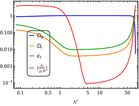
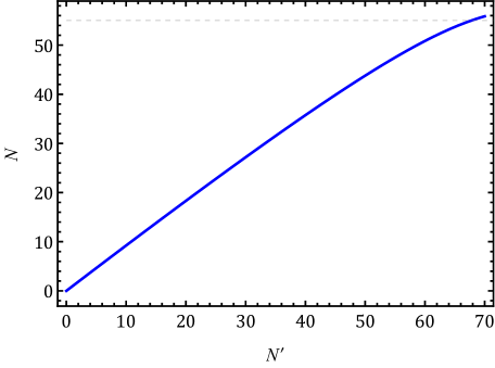
Figure 6: The evolution of cosmological variables for the case where $Q=5.0$ and the plot of $N$ with respect to $N^{\prime}$. For the entire inflationary regime we have checked that $T/H>1$.

The analysis of the constant $Q$ warm inflation shows that in this case also we can show the nature of the trajectories in the three dimensional phase space of the system. The compactified phase space show cylindrical symmetry and do show that many trajectories do get attracted towards an inflationary regime. In this section we have introduced all the relevant methods in which one can study the stability of warm inflationary systems of many more involved systems. Next we will try to see how the phase space dynamics of warm inflation in the constant $Q$ regime is modified when we apply the constant-roll condition. One must note that the modification will not in general correspond in a simple way to the unmodified case, presented here, because the form of the potential giving rise to CRWI will change from the one used here. Inspite of the different forms of the potentials we will be able to figure out how the new dynamics in CRWI differs from simple warm inflation dynamics.

5 Constant-roll warm inflation (CRWI)

In this section, we explore the constant-roll scenario in the framework of warm inflation. The constraint equation governing the constant-roll warm inflation, remains the same as introduced in Eq. (3.1):

$$\ddot{\phi}=-3\beta H\dot{\phi}\,.$$

In CRWI the Friedmann equations in Eq. (4.8) remain unchanged, however, the scalar field equation becomes a first order differential equation:

$$3H\dot{\phi}\left[(1+Q)-\beta\right]=-V_{,\phi}\,.$$ (5.1)

Here $Q=\Upsilon/3H$ as defined in the previous section on warm inflation. The constant-roll condition always acts like a dynamical constraint and turns the second order differential equation for the inflaton into a first order differential equation. This fact has interesting consequences as was observed in the case of CRCI where the dynamics of the system could be obtained from purely algebraic equations. We will like to see how warm inflation dynamics is affected by the constant-roll constraint. As in CRCI, in this case also we have different kind of inflaton potentials for positive and negative values of $\beta$.

It is known that in CRWI if $Q$ is a function of the inflaton field and the temperature then the dynamical system becomes ill defined [79] if one demands CRWI to be taking place near a dynamic thermal equilibrium. This difficulty arises because in such a case the thermal stability condition and the constant-roll condition combines to produce a scalar field solution which may not respect the Friedmann equations. Consequently, CRWI is a highly constrained system where only constant $Q$ is allowed. One may also work with a temperature dependent $Q$, but as thermal stability is assumed, we will have temperature to be approximately constant throughout the inflationary phase and consequently temperature dependent $Q$ also behaves a constant $Q$ system. These points are elaborately explained in Ref. [79]. Henceforth we address the various cases of CRWI corresponding to positive and negative values of $\beta$ respectively. We will only analyze the inflationary dynamics assuming constant $Q$.

5.1 CRWI with $\beta>0$ and constant $Q$

Constant-roll conditions affect the graceful exit problem in most inflationary theories. It is generally seen that many inflaton potentials which can cause inflation like behavior are not suitable as with those potentials the inflationary phase never ends. Graceful exit within this framework, for $\beta>0$, can be achieved with the inflaton potential given by [79]:

$$V(\phi)=V_{0}\left[\mathcal{A}\cosh^{2}{\left(\mathcal{B}\kappa(\phi_{0}-\phi)\right)}-1\right],$$ (5.2)

where $\mathcal{A}\equiv\dfrac{2(1+Q)-2\beta-3Q\beta}{2(1+Q)}$, $\mathcal{B}\equiv 3\sqrt{\frac{(1+Q)\beta}{6}}$, and $(\phi_{0},V_{0})$ are constants. It is observed that the constants $\mathcal{A},\mathcal{B}$ depends on the values of $Q$ and $\beta$. The variation of $\mathcal{A}$ and $\mathcal{B}$ is depicted in Fig. [7] for various values of $Q,\,\,\beta$.

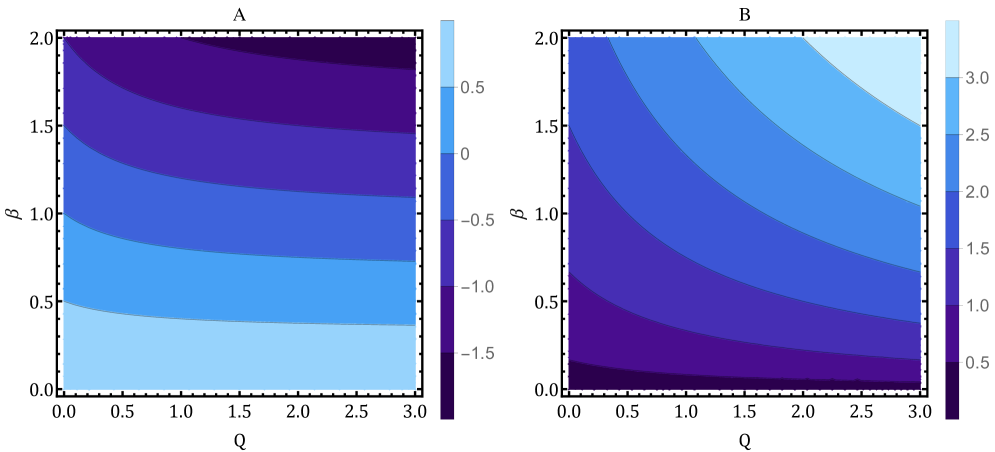
Figure 7: The variation of $\mathcal{A}$ and $\mathcal{B}$ in the parameter space of $(Q,\beta)$ when $\beta>0$.

From the plots, it is evident that $\mathcal{A}$ can take negative values for $\beta>1$ and $Q>0$, while $\mathcal{B}$ remains positive. However, $\mathcal{B}$ becomes complex for negative $\beta$, so negative values of $\beta$ are excluded.

To explore the dynamical scenario in this case, we define the dimensionless dynamical variables in a manner we have done so far for other cases:

$$x^{2}=\frac{{V}}{{3V_{0}}},\quad y=\frac{\dot{\phi}}{\sqrt{6}\sqrt{V_{0}}},\quad z=\frac{H}{\kappa\sqrt{V_{0}}}.$$ (5.3)

The other variables can be expressed in terms of the primary variables as:

$$\Omega_{r}=\frac{\kappa^{2}\rho_{r}}{3H^{2}}=\frac{\rho_{r}}{3z^{2}V_{0}},\quad\Omega_{\phi}=\frac{\kappa^{2}\rho_{\phi}}{3H^{2}}=\frac{x^{2}+y^{2}}{z^{2}}\ .$$ (5.4)

With these variables, the first Friedmann equation becomes:

$$1=\Omega_{\phi}+\Omega_{r}.$$ (5.5)

Similarly, the other important quantities, such as the slow-roll parameter and the thermal stability parameter, become:

$$\epsilon_{1}=\frac{-y^{2}-2z^{2}+2x^{2}}{z^{2}},\quad\frac{\dot{\rho}_{r}}{4\rho_{r}H}=\frac{3Qy^{2}}{2(z^{2}-x^{2}-y^{2})}-1\ .$$ (5.6)

One can see that the inflaton potential used in the present context is not positive definite but for inflation we will be working with a class of initial conditions and a particular set of parameter values for which $V(\phi)>0$. As because $V$ can be negative, we will have to work only with the positive or negative branch of $x$. Here we work with positive values of $x$. The primary variables $(x,z)$ can take any values within the range $[0,\infty)$. To keep track of the behavior of the variables at infinity we compactify the space spanned by these variables and define:

$$\bar{x}=\dfrac{x}{\sqrt{1+x^{2}}},\quad\bar{z}\equiv\dfrac{z}{\sqrt{1+z^{2}}}\,.$$ (5.7)

These transformations map the infinite interval to a finite interval $[0,1)$.

Using the variables defined in this section we can now construct the autonomous system of equations. From our previous discussion we know that in the present case we have two independent variables which can describe the dynamics of the system. The autonomous system of equations corresponding to the relevant variables $(\bar{x},\bar{z})$ are:

$$\bar{x}^{\prime} = -{y}\mathcal{A}\sqrt{(1+Q)\beta}\dfrac{(1-\bar{x}^{2})^{2}\sqrt{\frac{1}{\mathcal{A}}\dfrac{2\bar{x}^{2}+1}{1-\bar{x}^{2}}}\sqrt{\frac{1}{\mathcal{A}}\dfrac{2\bar{x}^{2}+1}{1-\bar{x}^{2}}-1}}{\bar{x}}\ ,$$ (5.8)

$$\bar{z}^{\prime} = \left(1-\bar{z}^{2}\right)^{\frac{3}{2}}\left(-y^{2}-2\dfrac{\bar{z}^{2}}{1-\bar{z}^{2}}+2\dfrac{\bar{x}^{2}}{1-\bar{x}^{2}}\right)\ .$$ (5.9)

Here, the derivative is defined as $()^{\prime}\equiv\frac{d()}{\kappa\sqrt{V_{0}}dt}$, and $y$ can be expressed in terms of $(\bar{x},\bar{z})$ using the relation

$$y=\mp\frac{2}{\sqrt{6}}\frac{\sqrt{1-\bar{z}^{2}}}{\bar{z}}\frac{\mathcal{A}\sqrt{\frac{(1+Q)\beta}{6}}}{\left((1+Q)-\beta\right)}\sqrt{\frac{1}{\mathcal{A}}\dfrac{2\bar{x}^{2}+1}{1-\bar{x}^{2}}}\sqrt{\frac{1}{\mathcal{A}}\dfrac{2\bar{x}^{2}+1}{1-\bar{x}^{2}}-1}\,.$$ (5.10)

Since the autonomous system of equations requires only two variables to fully describe the dynamics, the resulting phase space is two-dimensional. One must note that the first autonomous equation above explicitly depends on $y$ which has two branches, one positive and the other negative, clearly seen from Eq. (5.10). In the present case we have worked with the positive branch of $y$ as the results can be interpreted with ease in such a case.

Points	$(\bar{x}_{*},\bar{z}_{*})$	$\Omega_{\phi}$	$\epsilon_{1}$	$\frac{\dot{\rho}_{r}}{H\rho_{r}}$	Stability
$P_{1}$	$(0,0)$	$\infty$	$\infty$	$-\frac{3Q}{2}-1$	Unstable
$P_{2}$	$(1,1)$	Indeterminate	$2$	$-1$	Unstable
$P_{3}$	$(\rm{Any},1)$	$0$	$2$	$-1$	Unstable

Table 2: The critical points and their nature for CRWI Model when $\beta>0$.

It is important to note that the differential equation system diverges for $(\bar{x}=0,1)$ and $\bar{z}=0$. To address these divergences, we redefine the time variable as follows:

$$\kappa\sqrt{V_{0}}dt\to\kappa\sqrt{V_{0}}\bar{z}^{2}\bar{x}(1-\bar{x}^{2})^{2}d{t}\ .$$ (5.11)

The modified autonomous equations will become:

$$\bar{x}^{\prime} = -{y}\bar{z}^{2}\mathcal{A}\sqrt{(1+Q)\beta}{(1-\bar{x}^{2})^{4}\sqrt{\frac{1}{\mathcal{A}}\dfrac{2\bar{x}^{2}+1}{1-\bar{x}^{2}}}\sqrt{\frac{1}{\mathcal{A}}\dfrac{2\bar{x}^{2}+1}{1-\bar{x}^{2}}-1}}\ ,$$ (5.12)

$$\bar{z}^{\prime} = \bar{z}^{2}\bar{x}\left(1-\bar{z}^{2}\right)^{\frac{3}{2}}\left(-y^{2}-2\dfrac{\bar{z}^{2}}{1-\bar{z}^{2}}+2\dfrac{\bar{x}^{2}}{1-\bar{x}^{2}}\right)(1-\bar{x}^{2})^{2}\ .$$ (5.13)

Here, the derivative is defined as $()^{\prime}\equiv\frac{d()}{\kappa\sqrt{V_{0}}d{t}}$. To determine the qualitative behavior, we compute the critical points corresponding to the redefined equations. These critical points are summarized in Tab. [2]. The system yields three critical points, none of which depend on any model parameters.

At point $P_{1}$, both coordinates vanish, resulting in an indeterminate fractional energy density. Additionally, the slow-roll parameter becomes very large, rendering this point unstable.

At the point $P_{2}$ the field fractional energy density becomes indeterminate, and the slow-roll parameter exceeds 1. Upon evaluating their stability, the point $P_{2}$ exhibits unstable behavior for any choice of model parameters. Here the point $P_{3}$ is not representing any specific point, as $\bar{x}$ can take any value. Here $P_{3}$ actually represents a line of critical points where $\bar{x}\neq 1$. This line of critical points is generally unstable.

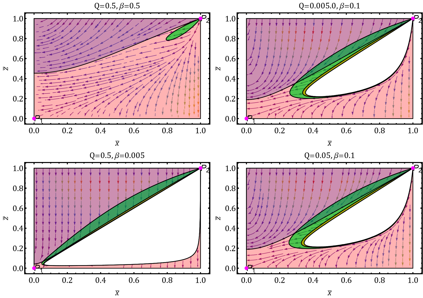
Figure 8: The phase space is corresponding to CRWI when $\beta>0$. The color scheme highlights the different dynamical regions: pink ($\epsilon_{1}\geq 1$), yellow region ($0\leq\epsilon_{1}\leq 0.1$), green region ($0.1<\epsilon_{1}<1$), blue (thermally stable region), and violet (overlap of red and blue regions).

The phase space is depicted in Fig. [8] for different values of $(Q,\beta)$ in the parameter space of $(\bar{x},\bar{z})$. The phase space is illustrated using distinct color regions: pink represents $\epsilon_{1}\geq 1$, green corresponds to $0.1<\epsilon_{1}<1$, yellow indicates $0\leq\epsilon_{1}\leq 0.1$, and violet denotes the thermally stable region. The white region represents an unphysical domain where $\epsilon_{1}$ becomes negative.

For $(Q=0.5,\beta=0.5)$, no physically viable dynamics exist. Conversely, for $\beta\ll 0.1$, as shown in the bottom left panel, trajectories originating from the line of critical points ($\bar{z}=1,\bar{x}\neq 1$) maintain thermal stability and are drawn towards the green region, eventually entering the yellow region, where the slow-roll condition $0\leq\epsilon_{1}\leq 0.1$ is satisfied. These physically viable trajectories exit the inflationary region and transition into the pink region maintaining thermal equilibrium, marking the end of inflation. Something similar happens in the lower right figure, but in this case the trajectories from the yellow region does not always remain in thermal equilibrium as they flow towards the pink region. In an overall manner, the dynamics of these trajectories confirm that CRWI can occur although the phase space of these processes is much more constrained and complicated.

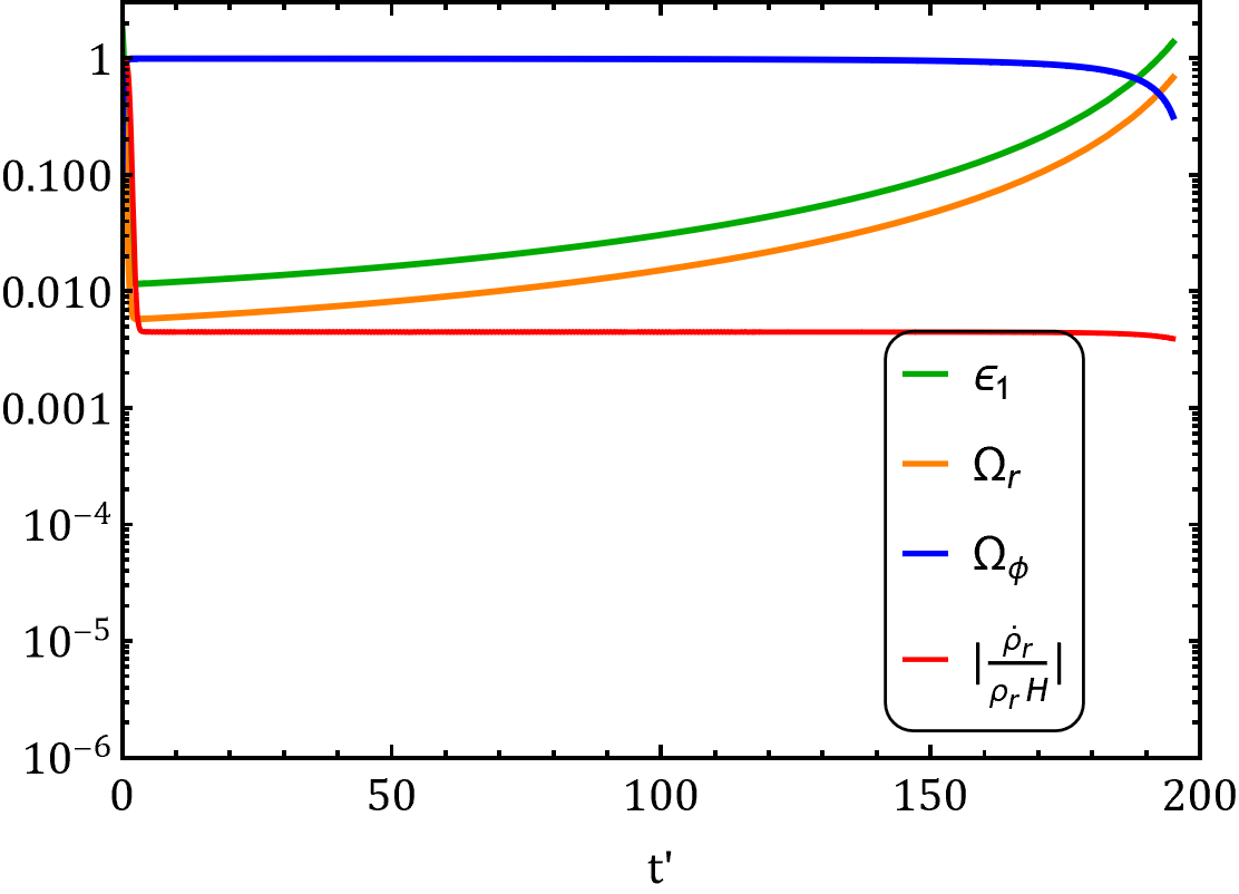
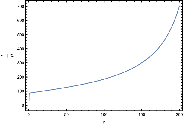
Figure 9: The evolution of CRWI corresponding variables and plot of $\frac{T}{H}$ of CRWI corresponding to $(Q=300,{\beta}=3\times 10^{-3})$ and $V_{0}=10^{-6}M^{4}_{\rm Pl}$.

If we follow one of the trajectories in the phase space we can construct the explicit inflationary dynamics which correspond to that trajectory. Here we plot the evolution of the cosmological parameters against the redefined time variable ${t^{\prime}}$ for $Q=300,\,\beta=3\times 10^{-3}$ in left panel of Fig. [9]. From the plot we can see that during the initial phase, the field energy density dominates over the radiation energy density, and the corresponding slow-roll parameter remains less than one. At around $t^{\prime}\sim 200$ the radiation energy density starts to dominate and inflation ends. At around this time we observe $\epsilon_{1}\sim 1$. On the right hand panel of Fig. [9], we show the evolution of $T/H$ during the inflationary period. It is clearly seen that during the inflationary period we have $T>H$ showing that thermal fluctuations dominate over quantum fluctuations.

As the radiation energy density starts to dominate, the slow-roll parameter exceeds 1, signaling the system’s exit from the inflationary phase after ${t^{\prime}}=195$ which corresponds to about 87 $e$-folds. It must be noted that by tuning the initial conditions one can reduce the number of $e$-folds. This tuning requires a detailed search in the initial condition space and parameter space of the theory. In this paper we present the method in principle and show that a through numerical stability analysis is possible in highly constrained inflationary systems. To calculate the number of e-folds, we use the formula: $N=\int H\,dt,$ which, in our case, can be expressed as:

$$N=\int H\,dt=\int\kappa\sqrt{V_{0}}z\,dt=\int\frac{\bar{z}}{\sqrt{1-\bar{z}^{2}}}\,dt^{\prime}.$$

Here, $\bar{z}$ is obtained by solving Eqs. (5.8–5.9) as a function of $t^{\prime}$. By integrating over the entire duration of inflation in terms of $t^{\prime}$, we determine the total number of $e$-folds. Throughout the evolution, the modulus of the thermal stability parameter remains less than 1, ensuring thermal stability during the entire process.

5.2 CRWI with $\beta<0$ and constant $Q$

In this case mostly all of the equations used to study the dynamics of the inflationary system remains the same as in the previous case except the constnt-roll condition. When $\beta<0$, the constraint equation for constant-roll can be written as:

$$\ddot{\phi}=3\tilde{\beta}H\dot{\phi},$$ (5.14)

where $\tilde{\beta}=-\beta$. When the constant roll parameter $\beta<0$, and during inflation the radiation energy density evolves slowly, constant-roll warm inflation is possible with the inflaton potential of the form described in Ref. [79]:

$$V(\phi)=V_{0}\left[1-\mathcal{\tilde{A}}\sin^{2}{\left(\mathcal{\tilde{B}}\kappa(\phi_{0}+\phi)\right)}\right]\,,$$ (5.15)

where $\mathcal{\tilde{A}}\equiv\dfrac{2\left(1+Q\right)+2\tilde{\beta}+3\tilde{\beta}Q}{2(1+Q)}$ and $\mathcal{\tilde{B}}\equiv 3\sqrt{\frac{(1+Q)\tilde{\beta}}{6}}$ and $Q$ is a constant. Notice that unlike the $\beta>0$ case here $\mathcal{\tilde{A}}$ and $\mathcal{\tilde{B}}$ are always positive quantities. The variation of $\mathcal{\tilde{A}}$ and $\mathcal{\tilde{B}}$ with $\tilde{\beta}$ and $Q$ is shown in Fig. [10]. As in the previous case, in the present case also the potential $V(\phi)$ is not positive definite. For our study of inflationary dynamics we will work with specific parameter values and some class of initial conditions which always keeps the potential positive.

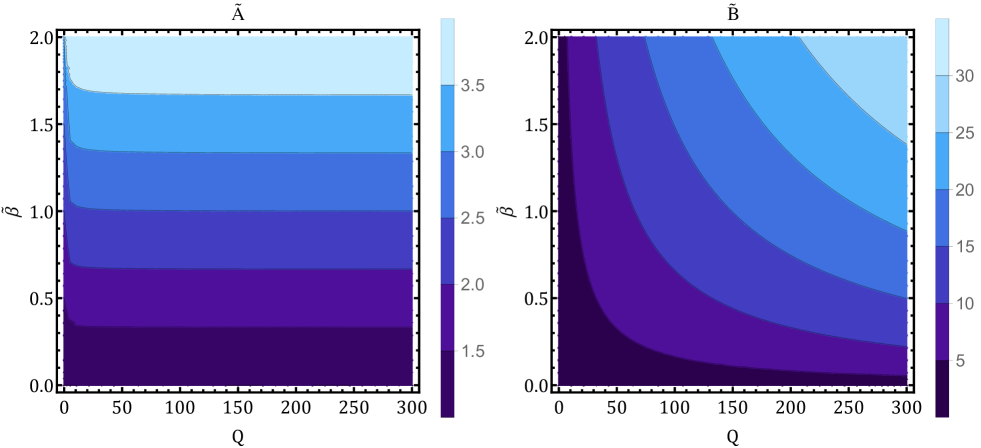
Figure 10: The variation of $\mathcal{\tilde{A}}$ and $\mathcal{\tilde{B}}$ in the parameter space of $(Q,\tilde{\beta})$ when $\beta<0$.

As established earlier, we adopt the dynamical variables $(x,y,z)$, $(\Omega_{r},\Omega_{\phi})$, and their compactified counterparts $(\bar{x},\bar{z})$ as defined in Eqs. (5.3)–(5.7). These definitions ensure a finite and well-behaved phase space, mapping infinities to the interval $[0,1)$, and will be used throughout the subsequent analysis. As in the previous case, we will only work with the positive branch of $x$.
The field $\phi$ can be expressed in terms of $\bar{x}$ as:

$$\frac{1}{\kappa\mathcal{\tilde{B}}}\arcsin\left(\sqrt{\frac{1}{\mathcal{\tilde{A}}}\dfrac{1-4\bar{x}^{2}}{1-\bar{x}^{2}}}\right)-\phi_{0} =\phi\,.$$ (5.16)

This condition imposes a constraint on $\bar{x}$, specifically $|\bar{x}|\leq\frac{1}{2}$. Here Eq. (5.16) and Eq. (5.15) jointly yield:

$$V_{,\phi}=2V_{0}\kappa\mathcal{\tilde{A}}\mathcal{\tilde{B}}\sqrt{\frac{1}{\mathcal{\tilde{A}}}\dfrac{1-4\bar{x}^{2}}{1-\bar{x}^{2}}}\sqrt{1-\frac{1}{\mathcal{\tilde{A}}}\dfrac{1-4\bar{x}^{2}}{1-\bar{x}^{2}}}\,.$$ (5.17)

The field equation for $\beta<0$ is:

$$3H\dot{\phi}(\tilde{\beta}+1+Q)=-V_{,\phi},$$ (5.18)

which gives

$$y=\pm\frac{2}{\sqrt{6}(\tilde{\beta}+1+Q)}\frac{\sqrt{1-\bar{z}^{2}}}{\bar{z}}\mathcal{\tilde{A}}\mathcal{\tilde{B}}\sqrt{\frac{1}{\mathcal{\tilde{A}}}\dfrac{1-4\bar{x}^{2}}{1-\bar{x}^{2}}}\sqrt{1-\frac{1}{\mathcal{\tilde{A}}}\dfrac{1-4\bar{x}^{2}}{1-\bar{x}^{2}}}\,.$$ (5.19)

Using Eq. (5.16) and the definition of $\bar{z}$, we obtain the autonomous equations in the present case as:

$$\bar{x}^{\prime} =\sqrt{6}y\mathcal{\tilde{A}}\mathcal{\tilde{B}}\frac{(1-\bar{x}^{2})^{2}}{3\bar{x}}\sqrt{\dfrac{(4\bar{x}^{2}-1)(1+\bar{x}^{2}(4-\mathcal{\tilde{A}})-\mathcal{\tilde{A}})}{(1-\bar{x}^{2})^{2}\mathcal{\tilde{A}}^{2}}}\,,$$ (5.20)

$$\bar{z}^{\prime} =\left(1-\bar{z}^{2}\right)^{\frac{3}{2}}\left(-y^{2}-2\dfrac{\bar{z}^{2}}{1-\bar{z}^{2}}+2\dfrac{\bar{x}^{2}}{1-\bar{x}^{2}}\right)\,,$$ (5.21)

where $y$ is given by Eq. (5.19), making the phase space two dimensional and where $()^{\prime}\equiv\frac{d()}{\kappa\sqrt{V_{0}}dt}$. We can see that $y$ has two branches, the positive and the negative ones. Here we have worked with the positive branch to illustrate the results. For warm inflation we need the radiation energy density $\rho_{r}>0$, i.e.

$$\frac{\rho_{r}}{3V_{0}}=\dfrac{\bar{z}^{2}}{1-\bar{z}^{2}}-\dfrac{\bar{y}^{2}}{1-\bar{y}^{2}}-\dfrac{\bar{x}^{2}}{1-\bar{x}^{2}}>0\,.$$ (5.22)

During the inflationary phase we need $\epsilon_{1}<1$ and we demand that inflation occurs near a dynamic thermal equilibrium, which translates to the condition: $\frac{|\dot{\rho}_{r}|}{4H\rho_{r}}<1$.

To analyze the behavior of the system, we utilize the autonomous system of equations previously constructed. The autonomous equations corresponding to the variables $(\bar{x},\bar{z})$ are given by Eq. (5.20) and Eq. (5.21). In the present case the autonomous system of equations diverges for $\bar{x}=0$ and $\bar{z}=0$. To address these divergences, we redefine the time variable as follows:

$$\kappa\sqrt{V_{0}}dt\to\kappa\sqrt{V_{0}}\bar{z}^{2}\bar{x}d{t}\,.$$ (5.23)

The modified autonomous equations are:

$$\bar{x}^{\prime} =\sqrt{6}y\mathcal{\tilde{A}}\mathcal{\tilde{B}}\frac{\bar{z}^{2}(1-\bar{x}^{2})^{2}}{3}\sqrt{\dfrac{(4\bar{x}^{2}-1)(1+\bar{x}^{2}(4-\mathcal{\tilde{A}})-\mathcal{\tilde{A}})}{(1-\bar{x}^{2})^{2}\mathcal{\tilde{A}}^{2}}}\,,$$ (5.24)

$$\bar{z}^{\prime} =\bar{z}^{2}\bar{x}\left(1-\bar{z}^{2}\right)^{\frac{3}{2}}\left(-y^{2}-2\dfrac{\bar{z}^{2}}{1-\bar{z}^{2}}+2\dfrac{\bar{x}^{2}}{1-\bar{x}^{2}}\right)\,.$$ (5.25)

Points	$(\bar{x}_{*},\bar{z}_{*})$	$\Omega_{\phi}$	$\epsilon_{1}$	$\frac{\dot{\rho}_{r}}{H\rho_{r}}$	Stability
$P_{1}$	$(0,0)$	$\infty$	$\infty$	$-\frac{3Q}{2}-1$	Unstable
$P_{2}$	$(\rm{Any},1)$	$0$	$2$	$-1$	Unstable

Table 3: The critical points and their nature for CRWI Model.

To determine the qualitative behavior of the dynamical system we compute the critical points corresponding to the redefined equations. These critical points are summarized in Tab. [3]. The system yields two critical points, none of which depend on any model parameters, including $\tilde{\beta}$. At point $P_{1}$, both coordinates vanish, resulting in an indeterminate inflaton fractional energy density. Additionally, the slow-roll parameter becomes very large, rendering this point unstable.

The points $P_{2}$ actually specifies a line of fixed points and these fixed points correspond to phases in the radiation dominated epoch, as $\Omega_{\phi}$ vanishes and the slow-roll parameter exceeds 1. Upon evaluating their stability, both the points $P_{1}$ and $P_{2}$ exhibit unstable nature for any choice of model parameters.

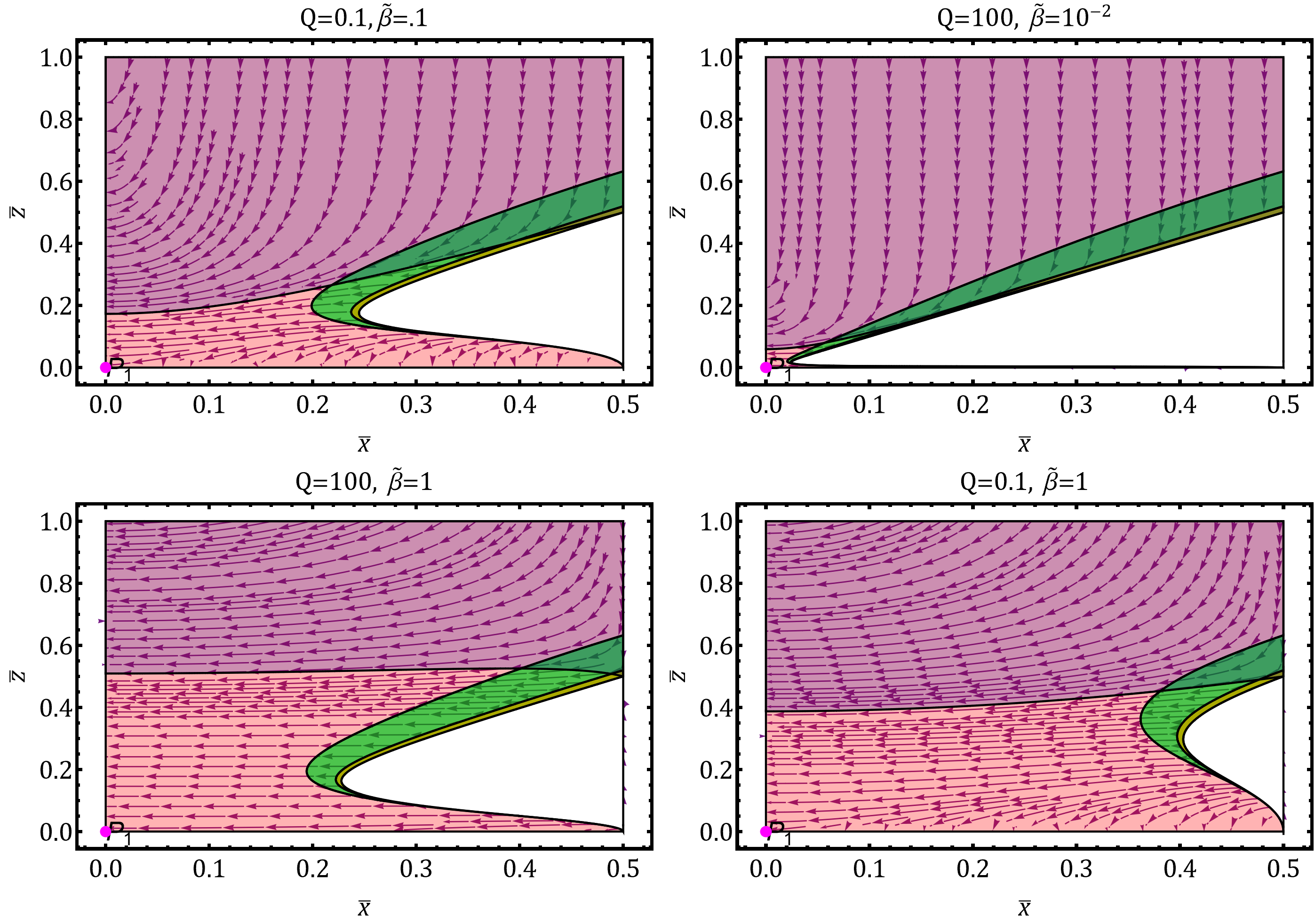
Figure 11: The phase space corresponding to CRWI with $\beta<0$. The color scheme highlights the different dynamical regions: pink ($\epsilon_{1}\geq 1$), yellow region ($0\leq\epsilon_{1}\leq 0.1$), green region ($0.1<\epsilon_{1}<1$), blue (thermally stable region), and violet (overlap of red and blue regions).

The phase space for the constant-roll warm inflation (CRWI) model is illustrated in Fig. [11] for various parameter choices of $(Q,\tilde{\beta})$ within the $(\bar{x},\bar{z})$ space. The phase space is depicted using distinct color codes: the pink region corresponds to $\epsilon_{1}\geq 1$, the yellow region corresponds to $0\leq\epsilon_{1}\leq 0.1$, the green region corresponds to $0.1<\epsilon_{1}<1$ and finally the blue region specifies the set of points in the phase space where we have thermal stability . Where the blue and red regions overlap, the color appears violet. Additionally, the white region represents areas where the slow-roll parameter is negative ($\epsilon_{1}<0$) and hence these regions are practically ruled out from any meaningful dynamical analysis. Since $\bar{z}=1$ corresponds to a line of unstable fixed points, Fig. [11] illustrates that trajectories diverge away from it. Additionally, the figure shows that all trajectories move toward $V=0$, i.e., the $\bar{x}=0$ line.

The plots on the lower panels show that when $\tilde{\beta}\gtrsim 1$, the thermally stable blue region has little to no overlap with the green or yellow regions, making CRWI practically impossible in these cases. In contrast, for the figures in the upper panels where $0<\tilde{\beta}\ll 1$, a substantial overlap between the blue and yellow regions ensures the existence of a thermally stable inflationary phase. In this favorable regime, the system’s trajectories originate from the critical points at $P_{2}$ (corresponding to the $\bar{z}=1$ line), traverses the inflationary epoch (highlighted in yellow), and eventually transitions into the inflationary region (green) while maintaining thermal stability at the radiation-dominated phase. This behavior closely resembles the dynamics observed for $\beta>0$, reinforcing the underlying qualitative consistency across these models.

We can choose one of the phase space trajectories to roughly figure out the inflationary dynamics in the present case. The temporal evolution of the cosmological parameters is shown in left hand panel of Fig. [12] for a representative parameter set $(Q=300,\tilde{\beta}=10^{-3})$. Initially, the field energy density dominates over the radiation energy density, resulting in the slow-roll parameter $\epsilon_{1}<1$, which confirms the system is within the inflationary phase. This plot shows a rough estimate of the inflationary process because we have shown the dynamics corresponding to a trajectory in the phase space and in this case we have not concentrated explicitly on the parameter choice and exact initial conditions which can produce an ideal inflationary phase. The right hand panel of Fig. [12] shows that throughout the inflationary phase we have $T>H$.

As the radiation energy density begins to dominate, the slow-roll parameter exceeds 1, marking the system’s exit from the inflationary regime after $t^{\prime}=320$ which corresponds to about 56 $e$-folds. A more robust choice of parameters and initial conditions may have increased the number of $e$-folds, but in this paper we do not specifically concentrate on the question of tuning the initial conditions and parameters. Throughout the evolution, the modulus of the thermal stability parameter remains less than 1, ensuring thermal stability is maintained during the entire process. This behavior is consistent with the corresponding analysis for $\beta>0$ case, emphasizing the robustness of the thermally stable inflationary dynamics in both parameterizations ($\beta\lessgtr 0$).

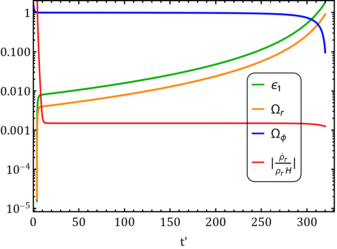
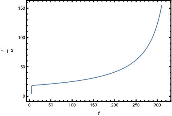
Figure 12: The dynamical evolution of various variables in CRWI and the evolution of $T/H$ during inflation corresponding to $(Q=300,\tilde{\beta}=10^{-3})$ and $V_{0}=10^{-4}M^{4}_{\rm Pl}$.

Comparing the phase space plots obtained in the various cases, in the present circumstance, with those obtained in the case of CRCI and WI, we see many differences. If we compare with the warm inflation case we see that unlike a cylindrical phase space we have a two dimensional phase space. Using compactified variables this two dimensional phase space becomes becomes closed and bounded. We see that in the present case a large part of the region inside the probable phase space becomes unphysical, as in those regions one gets a negative value of the slow-roll parameter $\epsilon_{1}$. The phase plots display a reduced number of trajectories which gives rise to a thermalized CRWI with graceful exit. For some parameter values we do not obtain any inflationary orbits. If we compare the phase orbits obtained in the present section with those obtained in the case of CRCI then we see CRWI is more restrictive. These feature is expected and apparent from the phase space behavior of the dynamical systems.

6 Conclusion

In this work we have tried to formulated a methodical approach to study the qualitative as well as the quantitative features of the phase space of the standard inflationary models and their constant-roll variants. To set the stage we began our investigation with the well-known cold inflationary scenario, considering a quadratic potential for the scalar field. Utilizing a Poincaré transformation, we compactified the system and identified that the only fixed point corresponds to the coordinates $(\phi,\dot{\phi})=(0,0)$. Notably, even if the system starts in a non-inflationary region, it transitions into the inflationary phase, characterized by $\epsilon_{1}\ll 1$, and eventually exits when $\epsilon_{1}\sim 1$. These results are consistent with findings reported in the literature. We have focused on a morphological study of the qualitative features of phase space in various cases of inflationary dynamics where all kinds of phase trajectories are present. We have not purely concentrated on trajectories which follow slow-roll inflation although in all cases we have shown that some slow-roll trajectories do exist for some parameters of the theory and for some class of initial conditions.

In our formulation of phase space dynamics of inflationary systems we have introduced the concept of compactified phases space to identify all the possible fixed points of the system and this method also gives a qualitative feature of the global behavior of the phase space. This construction turns out to be important in inflationary dynamics as inflation occurs for a very, very brief time period whereas the variables which describes the system ae defined in much longer timescale. In such a case one has to be sensitive about the presence of stable fixed points inside the inflationary regime, if such fixed points do exist then they can be dangerous for inflation. Consequently, for a proper inflationary dynamics one requires the stable fixed points to be in the asymptotic past or in the asymptotic future of the inflationary phase. Only unstable fixed points are allowed to exist in the regions of phase space where the slow-roll parameter $\epsilon_{1}<1$. The compactification scheme helps us to identify the fixed points at the asymptotic regions.

We have addressed the issue of singularities in the autonomous equations for the inflationary system. It has been shown that the singularities arising in the autonomous set of equations can be regulated by introducing a new time variable which is a monotonic increasing function of the old time variable. The regulation technique is mostly used in cosmological models of dark energy, for inflationary dynamics we have successfully used this powerful technique for the first time. We have shown that the duration of separation of events in the phase space do depend upon the choice of the time parameter. Using an inverse transformation one can go back to the standard time coordinates after the calculations are done. Using this technique we have found out the phase space dynamics in WI and CRWI.

Compared to standard cold inflation and warm inflation models, the constant-roll variants of these models are relatively constrained. The constraint comes from the constant-roll condition and is dynamic in nature. This dynamic constraint has appreciable effect on the dynamics as it drastically affects the dimension as well as the morphology of the phase space. The constant-roll condition directly affects the issue of graceful exit from inflation. Moreover the constant-roll condition transforms the dynamical system of CI into an algebraic system where one can figure out the phase space dynamics without explicitly solving any set of autonomous equations. Due to the constant-roll condition, the actual phase space of CRCI is one dimensional. To make the results more tractable we have plotted a recreated two dimensional stream-plot where the stramlines have phase space coordinateds in the case of CRCI. Compared to CRCI, CRWI has a genuine two dimensional phase space and CRWI can be tackled both algebraically as well as with the system of autonomous differential equations. In the present paper we have chosen the system of autonomous equations to study the dynamics of CRWI.

In the paper we have also established a standard method of studying stability analysis in the case of warm inflation. We present the result of warm inflation as it is a precursor of CRWI. We have dealt the case of warm inflation with utmost sensitivity as because the dynamics of the warm inflationary process is a delicate one as many conditions have to simultaneously satisfied during WI. These various conditions were discussed in the introduction. For the first time we have proposed a very general dynamical systems approach which can take care of all the subconditions in WI and produce the general structure of the phase space in WI. Using the knowledge gained in dealing the dynamical systems approach in WI we have modelled the produced the phase space structure of CRWI. Our work shows that the phase space of CRWI dynamics is nontrivial as due to various conditions applied on the system a part of the phase space remains dynamically unavailable.

Inflationary phenomenology is in general aimed at producing 60-70 $e$-folds of inflation and thereby producing cosmological perturbations so that structures can be formed in the later part of cosmological evolution. More emphasize is given to the calculation of power spectrum which is generated from various inflationary models and comparing those results with observational data. The dynamical stability and attractor nature of the background model in inflation is studied rarely. This study is very important as because the inevitability of cosmological inflation greatly depends upon the attractor nature of the inflationary processes in the phase space. In this paper we have introduced a thorough and methodical way to systematically study the dynamical structure and stability of the background inflationary models. We hope in the near future we will also be able to propose a methodical way to study the growth of inflationary perturbations.

Acknowledgement: The authors acknowledge professor Suratna Das’ comments regarding various points discussed in this paper.

References

- [1] D. Kazanas, Dynamics of the Universe and Spontaneous Symmetry Breaking, Astrophys. J. Lett., 241, (1980), L59.
- [2] A.H. Guth, The Inflationary Universe: A Possible Solution to the Horizon and Flatness Problems, Phys. Rev. D, 23, (1981), 347.
- [3] K. Sato, First Order Phase Transition of a Vacuum and Expansion of the Universe, Mon. Not. Roy. Astron. Soc., 195, (1981), 467.
- [4] K. Sato, Cosmological Baryon Number Domain Structure and the First Order Phase Transition of a Vacuum, Phys. Lett. B, 99, (1981), 66.
- [5] A.D. Linde, A New Inflationary Universe Scenario: A Possible Solution of the Horizon, Flatness, Homogeneity, Isotropy and Primordial Monopole Problems, Phys. Lett. B, 108, (1982), 389.
- [6] A. Albrecht and P.J. Steinhardt, Cosmology for Grand Unified Theories with Radiatively Induced Symmetry Breaking, Phys. Rev. Lett., 48, (1982), 1220.
- [7] A. Riotto, Inflation and the theory of cosmological perturbations, ICTP Lect. Notes Ser., 14, (2003), 317, [hep-ph/0210162].
- [8] V.F. Mukhanov, H.A. Feldman and R.H. Brandenberger, Theory of cosmological perturbations. Part 1. Classical perturbations. Part 2. Quantum theory of perturbations. Part 3. Extensions, Phys. Rept., 215, (1992), 203.
- [9] L.A. Urena-Lopez and M.J. Reyes-Ibarra, On the dynamics of a quadratic scalar field potential, Int. J. Mod. Phys. D, 18, (2009), 621, [0709.3996].
- [10] A.R. Liddle, P. Parsons and J.D. Barrow, Formalizing the slow-roll approximation in inflation, Physical Review D, 50, (1994), 7222–7232.
- [11] J.J.M. Carrasco, R. Kallosh and A. Linde, Cosmological attractors and initial conditions for inflation, Physical Review D, 92, (2015), .
- [12] A. Alho and C. Uggla, Quintessential -attractor inflation: a dynamical systems analysis, JCAP, 11, (2023), 083, [2306.15326].
- [13] C.G. Boehmer and N. Chan, Dynamical systems in cosmology., , (2017), DOI, [1409.5585].
- [14] C.G. Boehmer, N. Chan and R. Lazkoz, Dynamics of dark energy models and centre manifolds, Phys. Lett. B, 714, (2012), 11, [1111.6247].
- [15] S. Bahamonde, C.G. Böhmer, S. Carloni, E.J. Copeland, W. Fang and N. Tamanini, Dynamical systems applied to cosmology: dark energy and modified gravity, Phys. Rept., 775-777, (2018), 1, [1712.03107].
- [16] M. Bouhmadi-López, J.a. Marto, J.a. Morais and C.M. Silva, Cosmic infinity: A dynamical system approach, JCAP, 03, (2017), 042, [1611.03100].
- [17] A. Stachowski and M. Szydłowski, Dynamical system approach to running cosmological models, The European Physical Journal C, 76, (2016), .
- [18] A.A. Coley, Dynamical systems and cosmology, Kluwer, Dordrecht, Netherlands, (2003), 10.1007/978-94-017-0327-7.
- [19] A.D. Rendall, Cosmological models and center manifold theory, Gen. Rel. Grav., 34, (2002), 1277, [gr-qc/0112040].
- [20] J. Dutta, W. Khyllep and N. Tamanini, Dark energy with a gradient coupling to the dark matter fluid: cosmological dynamics and structure formation, JCAP, 01, (2018), 038, [1707.09246].
- [21] D.L. Blackmore, V.H. Samoylenko et al., Nonlinear dynamical systems of mathematical physics: spectral and symplectic integrability analysis, World Scientific, (2011).
- [22] U. Elias and H. Gingold, Critical points at infinity and blow up of solutions of autonomous polynomial differential systems via compactification, Journal of mathematical analysis and applications, 318, (2006), 305.
- [23] A. Chatterjee, S. Hussain and K. Bhattacharya, Dynamical stability of the k-essence field interacting nonminimally with a perfect fluid, Phys. Rev. D, 104, (2021), 103505, [2105.00361].
- [24] S. Hussain, S. Chakraborty, N. Roy and K. Bhattacharya, Dynamical systems analysis of tachyon-dark-energy models from a new perspective, Phys. Rev. D, 107, (2023), 063515, [2208.10352].
- [25] S. Hussain, A. Chatterjee and K. Bhattacharya, Dynamical stability in models where dark matter and dark energy are nonminimally coupled to curvature, Phys. Rev. D, 108, (2023), 103502, [2305.19062].
- [26] M. Saddam, Effects of non-minimal coupling of fluid and scalar field in cosmology, Ph.D. thesis, Indian Institute of Technology Kanpur,
- [27] S. Hussain, Non-adiabatic particle production scenario in algebraically coupled quintessence field with dark matter fluid, , 2403.10215.
- [28] S. Hussain, S. Nelleri and K. Bhattacharya, Comprehensive study of k-essence model: dynamical system analysis and observational constraints from latest Type Ia supernova and BAO observations, JCAP, 03, (2025), 025, [2406.07179].
- [29] S. Hussain, S. Arora, Y. Rana, B. Rose and A. Wang, Interacting models of dark energy and dark matter in Einstein scalar Gauss Bonnet gravity, JCAP, 11, (2024), 042, [2408.05484].
- [30] K. Bhattacharya, A. Chatterjee and S. Hussain, Dynamical stability in presence of non-minimal derivative dependent coupling of k-essence field with a relativistic fluid, Eur. Phys. J. C, 83, (2023), 488, [2206.12398].
- [31] E.J. Copeland, M. Sami and S. Tsujikawa, Dynamics of dark energy, Int. J. Mod. Phys. D, 15, (2006), 1753, [hep-th/0603057].
- [32] L. Kofman, A.D. Linde and A.A. Starobinsky, Reheating after inflation, Phys. Rev. Lett., 73, (1994), 3195, [hep-th/9405187].
- [33] L. Kofman, A.D. Linde and A.A. Starobinsky, Towards the theory of reheating after inflation, Phys. Rev. D, 56, (1997), 3258, [hep-ph/9704452].
- [34] R. Allahverdi, R. Brandenberger, F.-Y. Cyr-Racine and A. Mazumdar, Reheating in Inflationary Cosmology: Theory and Applications, Ann. Rev. Nucl. Part. Sci., 60, (2010), 27, [1001.2600].
- [35] B.A. Bassett, S. Tsujikawa and D. Wands, Inflation dynamics and reheating, Rev. Mod. Phys., 78, (2006), 537, [astro-ph/0507632].
- [36] A. Berera, Warm inflation, Phys. Rev. Lett., 75, (1995), 3218, [astro-ph/9509049].
- [37] V. Kamali, M. Motaharfar and R. O. Ramos, Recent Developments in Warm Inflation, Universe, 9, (2023), 124, [2302.02827].
- [38] A. Berera, I.G. Moss and R.O. Ramos, Warm Inflation and its Microphysical Basis, Rept. Prog. Phys., 72, (2009), 026901, [0808.1855].
- [39] M. Bastero-Gil, A. Berera, R.O. Ramos and J.G. Rosa, Warm Little Inflaton, Phys. Rev. Lett., 117, (2016), 151301, [1604.08838].
- [40] K.V. Berghaus, P.W. Graham and D.E. Kaplan, Minimal Warm Inflation, JCAP, 03, (2020), 034, [1910.07525].
- [41] A. Berera and L.-Z. Fang, Thermally induced density perturbations in the inflation era, Phys. Rev. Lett., 74, (1995), 1912, [astro-ph/9501024].
- [42] A. Berera, Thermal properties of an inflationary universe, Phys. Rev. D, 54, (1996), 2519, [hep-th/9601134].
- [43] M. Bastero-Gil, A. Berera, R.O. Ramos and J.G. Rosa, General dissipation coefficient in low-temperature warm inflation, Journal of Cosmology and Astroparticle Physics, 2013, (2013), 016–016.
- [44] A. Berera, The warm inflation story, Universe, 9, (2023), 272.
- [45] A. Berera, Warm inflation at arbitrary adiabaticity: A Model, an existence proof for inflationary dynamics in quantum field theory, Nucl. Phys. B, 585, (2000), 666, [hep-ph/9904409].
- [46] M. Bastero-Gil and A. Berera, Warm inflation model building, Int. J. Mod. Phys. A, 24, (2009), 2207, [0902.0521].
- [47] A.N. Taylor and A. Berera, Perturbation spectra in the warm inflationary scenario, Phys. Rev. D, 62, (2000), 083517.
- [48] L.M.H. Hall, I.G. Moss and A. Berera, Scalar perturbation spectra from warm inflation, Phys. Rev. D, 69, (2004), 083525.
- [49] I.G. Moss and T. Yeomans, Non-gaussianity in the strong regime of warm inflation, JCAP, 08, (2011), 009, [1102.2833].
- [50] I.G. Moss and C. Xiong, Non-Gaussianity in fluctuations from warm inflation, JCAP, 04, (2007), 007, [astro-ph/0701302].
- [51] B. Chen, Y. Wang and W. Xue, Inflationary non-gaussianity from thermal fluctuations, Journal of Cosmology and Astroparticle Physics, 2008, (2008), 014.
- [52] S. Gupta, A. Berera, A.F. Heavens and S. Matarrese, Non-Gaussian signatures in the cosmic background radiation from warm inflation, Phys. Rev. D, 66, (2002), 043510, [astro-ph/0205152].
- [53] H.P. de Oliveira and R.O. Ramos, Dynamical system analysis for inflation with dissipation, Phys. Rev. D, 57, (1998), 741, [gr-qc/9710093].
- [54] I.G. Moss and C. Xiong, On the consistency of warm inflation, JCAP, 11, (2008), 023, [0808.0261].
- [55] X.-B. Li, Y.-Y. Wang, H. Wang and J.-Y. Zhu, Dynamic analysis of noncanonical warm inflation, Phys. Rev. D, 98, (2018), 043510, [1804.05360].
- [56] S. Das, S. Hussain, D. Nandi, R. O. Ramos and R. Silva, Stability analysis of warm quintessential dark energy model, Phys. Rev. D, 108, (2023), 083517, [2306.09369].
- [57] S.D. Odintsov and T. Paul, From inflation to reheating and their dynamical stability analysis in Gauss–Bonnet gravity, Phys. Dark Univ., 42, (2023), 101263, [2305.19110].
- [58] R. D’Agostino and O. Luongo, Cosmological viability of a double field unified model from warm inflation, Phys. Lett. B, 829, (2022), 137070, [2112.12816].
- [59] X.-M. Zhang, R.-Q. Zhao, Z.-p. Peng, X.-B. Li, Y.-C. Feng, P.-C. Chu et al., Noncanonical warm inflation with nonminimal derivative coupling, JCAP, 02, (2025), 013, [2410.16839].
- [60] A. Jawad, S. Chaudhary and N. Videla, Dynamics of polynomial chaplygin gas warm inflation, Eur. Phys. J. C, 77, (2017), 808, [1711.03879].
- [61] H. Motohashi, A.A. Starobinsky and J. Yokoyama, Inflation with a constant rate of roll, Journal of Cosmology and Astroparticle Physics, 2015, (2015), 018–018.
- [62] Z. Yi and Y. Gong, On the constant-roll inflation, JCAP, 03, (2018), 052, [1712.07478].
- [63] M. Guerrero, D. Rubiera-Garcia and D. Saez-Chillon Gomez, Constant roll inflation in multifield models, Phys. Rev. D, 102, (2020), 123528, [2008.07260].
- [64] A. Mohammadi, N. Ahmadi and M. Shokri, On the constant roll complex scalar field inflationary models, JCAP, 06, (2023), 058, [2212.13403].
- [65] M. Shokri, J. Sadeghi and S.N. Gashti, Quintessential constant-roll inflation, Phys. Dark Univ., 35, (2022), 100923, [2107.04756].
- [66] W.-C. Lin, M.J.P. Morse and W.H. Kinney, Dynamical Analysis of Attractor Behavior in Constant Roll Inflation, JCAP, 09, (2019), 063, [1904.06289].
- [67] H. Motohashi and A.A. Starobinsky, f(r) constant-roll inflation, The European Physical Journal C, 77, (2017), .
- [68] H. Motohashi and A.A. Starobinsky, Constant-roll inflation: Confrontation with recent observational data, EPL (Europhysics Letters), 117, (2017), 39001.
- [69] S. Odintsov and V. Oikonomou, Inflation with a smooth constant-roll to constant-roll era transition, Physical Review D, 96, (2017), .
- [70] V.K. Oikonomou, Reheating in constant-roll f(r) gravity, Modern Physics Letters A, 32, (2017), 1750172.
- [71] Q. Gao, Reconstruction of constant slow-roll inflation, Science China Physics, Mechanics & Astronomy, 60, (2017), .
- [72] A. Ito and J. Soda, Anisotropic constant-roll inflation, The European Physical Journal C, 78, (2018), .
- [73] A. Karam, L. Marzola, T. Pappas, A. Racioppi and K. Tamvakis, Constant-roll (quasi-)linear inflation, Journal of Cosmology and Astroparticle Physics, 2018, (2018), 011–011.
- [74] F. Cicciarella, J. Mabillard and M. Pieroni, New perspectives on constant-roll inflation, Journal of Cosmology and Astroparticle Physics, 2018, (2018), 024–024.
- [75] L. Anguelova, P. Suranyi and L. Wijewardhana, Systematics of constant roll inflation, Journal of Cosmology and Astroparticle Physics, 2018, (2018), 004–004.
- [76] Q. Gao, The observational constraint on constant-roll inflation, Science China Physics, Mechanics & Astronomy, 61, (2018), .
- [77] Q. Gao, The observational constraint on constant-roll inflation, Science China Physics, Mechanics & Astronomy, 61, (2018), .
- [78] V. Kamali, M. Artymowski and M.R. Setare, Constant roll warm inflation in high dissipative regime, JCAP, 07, (2020), 002, [1905.04814].
- [79] S. Biswas, K. Bhattacharya and S. Das, Reassessing constant-roll warm inflation, Phys. Rev. D, 110, (2024), 063536, [2406.00340].
- [80] J. Martin and M. Musso, Solving stochastic inflation for arbitrary potentials, Phys. Rev. D, 73, (2006), 043516, [hep-th/0511214].
- [81] U. Elias and H. Gingold, Critical points at infinity and blow up of solutions of autonomous polynomial differential systems via compactification, Journal of Mathematical Analysis and Applications, 318, (2006), 305.
- [82] L. Barreira, J. Llibre and C. Valls, Bounded polynomial vector fields in r2 and rn, Journal of Differential Equations, 268, (2020), 4416.
- [83] J. Martin, H. Motohashi and T. Suyama, Ultra Slow-Roll Inflation and the non-Gaussianity Consistency Relation, Phys. Rev. D, 87, (2013), 023514, [1211.0083].
- [84] H. Motohashi and A.A. Starobinsky, Constant-roll inflation in scalar-tensor gravity, JCAP, 11, (2019), 025, [1909.10883].
- [85] M.J.P. Morse and W.H. Kinney, Large- constant-roll inflation is never an attractor, Phys. Rev. D, 97, (2018), 123519, [1804.01927].