Anchors no more:
Using peculiar velocities to constrain $H_{0}$ and the primordial Universe without calibrators

Abstract

We develop a novel approach to constrain the Hubble parameter $H_{0}$ and the primordial power spectrum amplitude $A_{\mathrm{s}}$ using supernovae type Ia (SNIa) data. By considering SNIa as tracers of the peculiar velocity field, we can model their distance and their covariance as a function of cosmological parameters without the need of calibrators like Cepheids; this yields a new independent probe of the large-scale structure based on SNIa data without distance anchors. Crucially, we implement a differentiable pipeline in JAX, including efficient emulators and affine sampling, reducing inference time from years to hours on a single GPU. We first validate our method on mock datasets, demonstrating that we can constrain $H_{0}$ and $\log 10^{10}A_{\mathrm{s}}$ within $\sim 10\%$ using $\sim 10^{3}$ SNIa. We then test our pipeline with SNIa from an $N$-body simulation, obtaining 7%-level unbiased constraints on $H_{0}$ with a moderate noise level. We finally apply our method to Pantheon+ data, constraining $H_{0}$ at the 10% level without Cepheids when fixing $A_{\mathrm{s}}$ to its $\it{Planck}$ value. On the other hand, we obtain 15%-level constraints on $\log 10^{10}A_{\mathrm{s}}$ in agreement with $\it{Planck}$ when including Cepheids in the analysis. In light of upcoming observations of low redshift SNIa from the Zwicky Transient Facility and the Vera Rubin Legacy Survey of Space and Time, surveys for which our method will develop its full potential, we make our veloce code publicly available. github

1 Introduction

Supernovae type Ia (SNIa) are the best standard candles in cosmology up to date. They have been instrumental in detecting the accelerated expansion of the Universe [1, 2] and supporting the dark energy hypothesis [3]. Within the standard flat $\Lambda$CDM cosmology, the recent expansion history is determined by the matter density $\Omega_{\rm{m}}$ and Hubble constant $H_{0}$, which can be both inferred from the luminosity distance-redshift relation $d_{\textrm{L}}(z)$ in a Friedmann-Lemaître (FL) universe. For this reason, SNIa are important for joint measurements of $H_{0}$ and $\Omega_{\rm{m}}$, see e.g. Ref. [4].

However, SNIa are not perfect standard candles, and they need to be normalized with the help of distance anchors; in particular, the Hubble constant is perfectly degenerate with the absolute distance normalization. Moreover, the Universe is not a perfect FL universe, but its matter distribution and geometry are perturbed, while the redshifts of SNIa are affected by the peculiar velocities of their host galaxies. So far, these velocities have mostly been modeled using the velocity field reconstruction approach to convert the CMB-corrected redshifts into so called ‘Hubble diagram redshifts’, $z_{\rm HD}$ [5].

In this work, we consider a different approach to treat velocities, based on Ref. [6]. We correct the SNIa redshifts for peculiar velocities by adding them to the velocity power spectrum covariance. Like the matter power spectrum, this covariance also depends on the cosmological parameters $H_{0}$ and $\Omega_{\rm{m}}$, in addition to the initial power spectrum described by the amplitude $A_{\rm{s}}$ and the spectral slope $n_{\rm{s}}$. The variance of the SNIa data therefore also contains information about $H_{0}$ which is completely independent of any distance anchor like the Cepheids. This is particularly interesting in light of the so-called Hubble tension [7, 8] as it provides an additional independent way to measure the low-redshift Hubble constant from supernova data.

Other works have looked into constraining the growth of structure from the power spectrum of peculiar velocities, using both simulated and real data. For instance, in Ref. [9] the authors used both simulated data and various real datasets like the COMPOSITE catalogue [10] to estimate the matter power spectrum, finding good agreement with $\Lambda$CDM, while Ref. [11] constrained the growth rate of structures using the 6dF Galaxy Survey [12]. A similar analysis was performed in Ref. [13] using the 2MASS Tully–Fisher survey [14]. In Ref. [15] a forecast of the constraints of the growth rate for ZTF (Zwicky Transient Facility, [16]) was performed using the FLIP package [17], while in Ref. [18] the impact of peculiar velocities on the measure of $H_{0}$ for the ZTF second data release [19] was estimated. The velocity power spectrum also proved to be useful in testing the standard cosmological model assuming distinct estimates of the matter density, as done in Ref. [20].

In our work, we specifically focus on $H_{0}$ and $A_{\textrm{s}}$, with a detailed treatment of the velocity covariance. We develop an efficient and differentiable pipeline that combines neural network emulators and affine sampling, and we validate it on mock data and $N$-body simulations. We finally apply our pipeline to Pantheon+ data [21], showing that in principle supernova surveys can constrain the Hubble parameter without the need for distance anchors. While results from present data are not yet conclusive, we envision that our method will fully unlock its potential with upcoming data like ZTF which include thousands of low-redshift SNIa [19].

This paper is structured as follows. In Sec. 2 we describe our theoretical model, while in Sec. 3 we present the implementation pipeline. We then validate our approach on a mock dataset, before applying it to an $N$-body simulation as well as to the Pantheon+ data, in Sec. 4. We conclude in Sec. 5.

2 Theoretical model

We model the SNIa magnitude data with a Gaussian likelihood, which is given by:

$$\log(\mathcal{L})=-\frac{1}{2}\biggl{[}\Delta\mu_{n}\,C^{-1}_{mn}\,\Delta\mu_{m}+\log({\rm det}\,C_{mn})+k\log(2\pi)\biggr{]},$$ (2.1)

where a summation over the repeated indices $m$ and $n$ is implied, and $k$ is the dimension of the covariance $C$, namely the number of SNIa in our dataset. The vector $\Delta\mu_{i}$ is given by:

$$\Delta\mu_{n}=\begin{cases}\mu_{n}-\mu_{{\rm ceph},n}+\delta M&\text{if}\ n\text{-th SNIa galaxy hosts Cepheids,}\\ \mu_{n}-\mu_{\mathrm{model}}(z_{n}^{\rm hel})+\delta M&\text{otherwise. }\end{cases}$$ (2.2)

Here, $\mu_{n}$ is the observed magnitude of the $n$-th SNIa, and $\delta M$ is a normalization parameter, i.e. the magnitude shift. SNIa in galaxies that also host Cepheids (providing a measurement of their normalized magnitude $\mu_{\rm ceph}$) are uniquely used to determine $\delta M$ which would otherwise be perfectly degenerate with $H_{0}$. The theoretical distance modulus $\mu_{\rm model}$ is related to the luminosity distance via:

$$\mu_{\mathrm{model}}=5\log_{10}\biggl{(}\frac{\langle d_{\mathrm{L}}(z^{\rm hel},{\mathbf{n}})\rangle}{\rm Mpc}\biggr{)}+25\,,$$ (2.3)

where

$$d_{\mathrm{L}}(z^{\rm hel},{\mathbf{n}})=\bar{d}_{\mathrm{L}}(z)\left[1+\frac{(1+z^{\rm hel})^{2}}{H(z^{\rm hel})\bar{d}_{\mathrm{L}}(z^{\rm hel})}{\mathbf{n}}\cdot({\mathbf{v}}_{\odot}-{\mathbf{v}}(z^{\rm hel},{\mathbf{n}}))-\frac{{\mathbf{n}}\cdot{\mathbf{v}}(z^{\rm hel},{\mathbf{n}})}{c}+\cdots\right]\,,$$ (2.4)

is the observable luminosity distance, with $z^{\rm hel}$ the measured heliocentric redshift, ${\mathbf{v}}_{\odot}$ the peculiar velocity of the solar system (measured by the CMB dipole), ${\mathbf{n}}$ the direction of the SNIa and ${\mathbf{v}}(z,{\mathbf{n}})$ its peculiar velocity. Furthermore, $H(z)=\dot{a}/a$ is the Hubble parameter, $a$ is the scale factor, and $\bar{d_{\mathrm{L}}}$ is defined in Eq. (2.6). The second and third terms in parentheses are the dominant terms at low redshift, while the full formula evaluating $\cdots$ at first order in perturbation theory is derived in Ref. [22]; these additional terms are relevant only at redshifts $z\gtrsim 0.3$, and here we will include only the dominant lensing term as an additional contribution to the variance.

When taking the ensemble average of Eq. (2.4) in terms of the CMB-corrected redshift $z=z^{\textrm{hel}}-(1+z){\mathbf{v}}_{\odot}\cdot{\mathbf{n}}/c$ (i.e. correcting $z^{\rm hel}$ for the observer motion, with $c$ ths speed of light), we find:

$$\langle d_{\mathrm{L}}(z,{\mathbf{n}})\rangle=\bar{d}_{\mathrm{L}}(z)\,.$$ (2.5)

$\bar{d}_{\mathrm{L}}(z)$ is the background luminosity distance, which in a flat $\Lambda$CDM model at late times is given by:

$$\bar{d}_{\mathrm{L}}(z)=(1+z)\!\int_{0}^{z}\!\!\frac{dz^{\prime}}{H(z^{\prime})}=\frac{1+z}{H_{0}}\!\int_{0}^{z}\!\frac{dz^{\prime}}{\sqrt{\Omega_{{\rm m}}(1+z^{\prime})^{3}+1-\Omega_{{\rm m}}}}=(1+z)r(z)\,,$$ (2.6)

where $r(z)$ is the comoving distance out to redshift $z$.

Even though the ensemble average of $d_{L}(z)$ is $\bar{d}_{L}(z)$, the measured $d_{\mathrm{L}}(z)$ does not simply average to $\bar{d}_{\mathrm{L}}(z)$, but as we have shown in a previous paper [23], it contains an additional monopole, dipole (the bulk velocity) and quadrupole. These additional contributions are not unexpected and are in good agreement with $\Lambda$CDM, as we have shown in Ref. [23]; they would average out in a true ensemble average over many universes, but they do not average out in the data. Therefore, in our estimator for $\bar{d}_{\mathrm{L}}(z)$ in the case of real supernova data we subtract the maximum-a-posteriori monopole, dipole and quadrupole terms using the scoutpip package.

We write the total covariance matrix $C$ as a sum of an error term, $C^{\rm(e)}_{mn}$ coming from measurement errors in the SNIa magnitudes, and a velocity-induced term, $C^{\rm(v)}_{mn}$, that describes the redshift fluctuations due to peculiar velocities:

$$C_{mn}=C^{\rm(e)}_{mn}+C^{\rm(v)}_{mn}\,.$$ (2.7)

The error covariance matrix $C^{\rm(e)}$ is the the error covariance of the SNIa data from which the peculiar velocity contribution is subtracted, while the velocity-induced covariance matrix $C^{\rm(v)}$ is due to the difference between the measured redshift $z_{n}$ and the redshift of the background cosmology $\bar{z}_{n}$ induced by peculiar velocities. This leads to a difference $\delta z_{n}=(1+z_{n})\frac{v_{n}}{c}$ between the measured and the cosmological redshift, where $v_{n}={\mathbf{n}}_{n}\cdot{\mathbf{v}}_{n}$ is the peculiar velocity of the $n$-th object. Here we include this redshift change as an additional fluctuation $\delta\mu_{n}^{(v)}$ of the distance modulus [15] given by:

$$\frac{\log{10}}{5}\delta\mu_{n}^{(\rm{v})}=\biggl{[}\frac{c(1+z_{n})^{2}}{d_{\textrm{L}}(z_{n})\,H(z_{n})}-1\biggr{]}\frac{v_{n}}{c}\,.$$ (2.8)

In Appendix A we derive and discuss in detail this result, which is in agreement with Ref. [15],

To obtain the velocity-induced covariance for the magnitudes, we start by considering the covariance of the radial component of the peculiar velocities. In our treatment, we neglect vorticity and first consider the linear velocity power spectrum from scalar perturbations, $P_{\textrm{v}}$. The covariance matrix of peculiar radial velocities is then of the form:

$$C^{\rm(v),v}_{mn} =\int\frac{4\pi k^{2}\mathrm{d}k}{(2\pi)^{3}}W_{mn}(k)\,\langle v_{m}v_{n}\rangle=\int\frac{4\pi k^{2}\mathrm{d}k}{(2\pi)^{3}}W_{mn}(k)\,P_{\rm v}\,(k,z_{m},z_{n})\,,$$ (2.9)

where $P_{\rm v}\,(k,z_{m},z_{n})$ is the unequal-redshift velocity power spectrum and $W_{mn}$ is a window function determined by the real space positions of the supernovae. To obtain the velocity-induced covariance matrix for the distance modulus $\mu_{i}$, we multiply Eq. (2.9) with the conversion factor $B_{mn}$ obtained from Eq. (2.8):

$$B_{mn}=\biggl{(}\frac{5}{c\,\log(10)}\biggr{)}^{2}\biggl{[}\frac{c(1+z_{m})^{2}}{d_{\mathrm{L}}(z_{m})\,H(z_{m})}-1\biggr{]}\biggl{[}\frac{c(1+z_{n})^{2}}{d_{\mathrm{L}}(z_{n})\,H(z_{n})}-1\biggr{]}\,.$$ (2.10)

The covariance of the SNIa magnitudes from peculiar velocities is then:

$$C^{\rm(v)}_{mn}=B_{mn} \int\frac{4\pi k^{2}\mathrm{d}k}{(2\pi)^{3}}W_{mn}(k)\,P_{\rm v}\,(k,z_{m},z_{n})$$ (2.11)

where the window function $W_{mn}$ in Eq. (2.11) is given by:

$$W_{mn}(k)=\sum_{i,j=1}^{3}n_{m,i}\,n_{n,j}\int\frac{\mathrm{d}^{2}\hat{k}}{4\pi}\hat{k}_{i}\,\hat{k}_{j}e^{ik\hat{\mathbf{k}}\cdot(\mathbf{r}_{m}-\mathbf{r}_{n})}\,,$$ (2.12)

with ${\mathbf{n}}_{m}={\mathbf{r}}_{m}/r_{m}$ and ${\mathbf{n}}_{n}={\mathbf{r}}_{n}/r_{n}$ the directions of the $m$-th and $n$-th SNIa respectively, and $i,j$ the spatial indexes. In Appendix B we derive an analytic expression for this window function:

$$W_{mn}(k)= \frac{1}{3}\cos{\alpha_{mn}}\left[j_{0}(kR_{mn})-2j_{2}(kR_{mn})\right]+\frac{r_{m}r_{n}}{R_{mn}^{2}}j_{2}(kR_{mn})\sin^{2}{\alpha_{mn}}\,,$$ (2.13)

where $\alpha_{mn}$ is the angle between $\mathbf{r}_{m}$ and $\mathbf{r}_{n}$, $j_{\ell}$ is $\ell$-th order spherical Bessel function and $R_{mn}=|\mathbf{r}_{m}-\mathbf{r}_{n}|$. For $m=n$ we have $W_{mm}=1/3$. These results agree with the more involved derivation given in Ref. [24].

2.1 The velocity power spectrum

Considering only linear perturbations, the velocity power spectrum $P_{\rm v}$ is given by:

$$P_{\rm v}(k,z_{m},z_{n})=\biggl{[}\frac{H(z_{m})f(z_{m})}{(1+z_{m})}\biggr{]}\biggl{[}\frac{H(z_{n})f(z_{n})}{(1+z_{n})}\biggr{]}\frac{P_{\delta}(k,z_{m},z_{n})}{k^{2}}\,,$$ (2.14)

where $P_{\delta}(k)$ is the linear matter power spectrum and $f(z)=H^{-1}(z)\dot{D}_{1}(z)/D_{1}(z)$ is the growth rate; $D_{1}$ is the linear growth function. In a flat $\Lambda$CDM cosmology it is given by [25]:

$$D_{1}(z)=\frac{1}{5\,(1+z)\,\Omega_{{\rm m}}(0)}\left[{}_{2}F_{1}\left(\frac{1}{3},1;\frac{11}{6};1-\frac{1}{\Omega_{\text{m}}(z)}\right)\right],$$ (2.15)

where ${}_{2}F_{1}(a,b;c;d)$ is the confluent hypergeometric function [26] and

$$\Omega_{{\rm m}}(z)=\frac{\Omega_{{\rm m}}\,(1+z)^{3}}{\Omega_{{\rm m}}\,(1+z)^{3}+(1-\Omega_{{\rm m}})}\,.$$ (2.16)

In order to take into account unequal time correlations of the matter power spectrum, we use the approximation described in Ref. [27], according to which:

$$P_{\delta}(k,z_{m},z_{n})=\mathcal{Z}(k,z_{m},z_{n})\,P_{\delta}(k,\bar{z})\,,$$ (2.17)

with

$$\mathcal{Z}(k,z_{m},z_{n})=e^{-(k/k_{\rm NL})^{2}[D_{1}(z_{m})-D_{1}(z_{n})]^{2}}\,$$ (2.18)

and the mean redshift $\tilde{z}$ is defined by

$$D_{1}(z_{m})D_{1}(z_{n})=D^{2}_{1}(\tilde{z})\,.$$ (2.19)

The $\mathcal{Z}(k,z_{m},z_{n})$ prefactor depends also on the non-linearity scale $k_{\rm NL}$ given by:

$$k_{\rm NL}^{-2}=\frac{1}{12\pi^{2}}\int_{0}^{\infty}P_{\delta}(k,0)\,\mathrm{d}k\,.$$ (2.20)

Using Eq. (2.19), we can rewrite Eq. (2.17) as:

$$P_{\delta}(k,z_{m},z_{n})=\mathcal{Z}(k,z_{m},z_{n})\,D_{1}(z_{m})D_{1}(z_{n})P_{\delta}(k,0)\,.$$ (2.21)

Combining everything, we obtain the following expression for the velocity covariance:

$$C^{\rm(v)}_{mn}= \frac{B_{mn}}{2\pi^{2}}\frac{D_{1}(z_{m})~D_{1}(z_{n})}{D_{1}^{2}(0)}\biggl{[}\frac{H(z_{m})f(z_{m})}{(1+z_{m})}\biggr{]}\biggl{[}\frac{H(z_{n})f(z_{n})}{(1+z_{n})}\biggr{]}$$ (2.22)

$$\int\mathrm{d}kW_{mn}(k)\mathcal{Z}(k,z_{m},z_{n})P_{\delta}(k,0)\,.$$

We compute the linear power spectrum using CAMB [28] up to $k_{\max}=100\ h/$Mpc.

In our analysis we have found that the unequal time decoherence factor $\mathcal{Z}(k,z_{m},z_{n})$ does not significantly impact the results. This is understood by the fact that supernovae that are at sufficiently different redshifts such that $D_{1}(z_{m})-D_{1}(z_{n})$ is appreciable are so far apart that the power spectrum $P_{\delta}(k)$ is very small for these $k$ values. We note that without $\mathcal{Z}(k,z_{m},z_{n})$, $H_{0}$ and $A_{\mathrm{s}}$ are perfectly degenerate in the linear velocity power spectrum, $P_{\rm{v}}$.

2.1.1 The non-linear velocity power spectrum

We further consider phenomenological corrections to the linear power spectrum, following Refs. [29, 30]. We define the non-linear velocity power spectrum $P^{\rm{NL}}_{\rm v}$ as:

$$P^{\rm{NL}}_{\rm v}(k,z_{m},z_{n})=P_{\rm v}(k,z_{m},z_{n})\,D_{\rm u}^{2}(k\sigma_{\rm u})\,E(\sigma_{8})\,,$$ (2.23)

with

$$D_{\rm u}(k\sigma_{u})={\rm sinc}({k\sigma_{u}})$$ (2.24)

a damping function correction introduced in Ref. [29], and $E(\sigma_{8})$ an extra non-linear correction with $3\%$ accuracy for $k<0.7\ h{\rm Mpc}^{-1}$ given by [30]:

$$E(\sigma_{8})=e^{-k\left[a_{1}(\sigma_{8})+a_{2}(\sigma_{8})k+a_{3}(\sigma_{8})k^{2}\right]}\,.$$ (2.25)

We fix $\sigma_{u}=13\ h^{-1}$Mpc, following Ref. [29]. The coefficients $a_{i}$ are linear functions of the root-mean-square of matter density fluctuations $\sigma_{8}$,

$$a_{1}(\sigma_{8}) =(-0.817+3.198\,\sigma_{8})\,{\rm Mpc}/h\,,$$ (2.26)

$$a_{2}(\sigma_{8}) =(0.877-4.191\,\sigma_{8})\,{\rm Mpc}^{2}/h^{2}\,,$$ (2.27)

$$a_{3}(\sigma_{8}) =(-1.199+4.629\,\sigma_{8})\,{\rm Mpc}^{3}/h^{3}\,.$$ (2.28)

At fixed $n_{\textrm{s}}$, $\sigma_{8}$ is proportional to $A_{\mathrm{s}}$ and given by:

$$\sigma_{8}=(\sigma_{8,{\it{Planck}}}\,/A_{\rm s,{\it Planck}})A_{\mathrm{s}}\,,$$

where for $\sigma_{8,{\it Planck}}=0.8102$ and $A_{\mathrm{s,\it Planck}}=10^{-10}\exp(3.047)=2.105\times 10^{-9}$ we choose the fiducial values from Planck (TT,TE,EE+lowE+lensing+BAO) [31]. Furthermore, we set $n_{\mathrm{s}}=0.965$ and the baryon density parameter $\omega_{\mathrm{b}}=0.02242$.

While the linear velocity power spectrum is proportional to $H_{0}^{2}A_{\mathrm{s}}$ and therefore $H_{0}$ and $A_{\mathrm{s}}$ are perfectly degenerate, this is no longer the case in the non-linear power spectrum as $E(\sigma_{8})$ depends on $A_{\mathrm{s}}$ but not on $H_{0}$. However, as we shall see in Section 4, the presently available data still show a very severe degeneracy between the value of $H_{0}$ inferred from the velocity covariance and $A_{\mathrm{s}}$.

2.2 Velocity dispersion

The velocity power spectrum gives in principle the non-linear peculiar velocity field as determined with $N$-body simulations. However, measuring this field with a finite, relatively small number of tracers adds a velocity dispersion [32, 33] which we take into account in the form:

$$C_{mn}^{\rm(v),disp}=B_{mn}\sigma_{\rm disp}^{2}\delta_{mn}\,,$$ (2.29)

only for those galaxies not hosting a Cepheid. The factor $B_{mn}$ again converts the velocity variance into a magnitude variance. We leave the value of $\sigma_{\rm disp}$ free in our analysis.

3 Methodology

We develop a differentiable Markov chain Monte Carlo (MCMC) pipeline combining efficient emulators and an affine sampler, running on a single graphics processing unit (GPU) and converging $10^{5}$ times faster than traditional approaches. The emulators’ ranges are reported in Table 1, which also includes the prior ranges for the MCMC analyses.

3.1 Pipeline description

The integral in Eq. (2.22) (with $P_{\mathrm{v}}$ replaced by the non-linear velocity power spectrum, $P_{\mathrm{v}}^{\mathrm{NL}}$) is computationally expensive: assuming a dataset containing $10^{3}$ objects, we need to compute it for all $\sim 5\cdot 10^{5}$ unique pairs of objects in the dataset at each likelihood evaluation. For each choice of cosmological parameters, i.e. for each step of the MCMC, this requires more than half million evaluations of the integral, with the number increasing quadratically with the number of objects in the survey. For this reason, we develop an emulator to evaluate the integral, computing each element of the covariance matrix using a neural network based on the CosmoPower emulation framework [34].

We first randomly select one million combinations of redshift pairs and angles from the Pantheon+ dataset, and concatenate them with cosmological parameters sampled uniformly from the ranges indicated in Table 1, which also act as the priors for the inference step. We compute the value of the integral using the FFTLog algorithm to account for the Bessel functions [35, 36], separating between the case $\alpha_{mn}=0$ (which does not involve Bessel integrals) and $\alpha_{mn}\neq 0$. We then train two emulators (one for $\alpha_{mn}=0$ and one for $\alpha_{mn}\neq 0$) to predict the value of the integral given the values of $z_{1}$, $z_{2}$, $\alpha_{12}$, $\Omega_{\rm{m}}$, $H_{0}$ and $\log\left(10^{10}A_{\rm{s}}\right)$, using a mean absolute error loss function to be robust to outliers. We find that each emulator converges in a few hours on a single GPU with a median performance at the sub-percent level on held-out test data, so we are confident that its predictions are accurate. We note that our emulators are trained on redshifts and angles drawn from the Pantheon+ dataset, so in principle one would need to train again in case a new dataset is considered; however, we tested that the performance was still satisfactory even on the $N$-body simulation data we consider in this paper. In future work, we will explore a more general emulator trained on a uniform distribution of redshifts and angles, which should be applicable to a wider variety of datasets.

Table 1: Prior distributions of the parameters for the training of the emulator (first three columns), and for inference (all columns). Uniform distributions are indicated with $\mathcal{U}$.

Parameter	$\Omega_{\rm{m}}$	$H_{0}$	$\log\left(10^{10}A_{\rm{s}}\right)$	$\log_{10}(\sigma_{\textrm{disp}}^{2})$	$\delta M$
Prior range	$\mathcal{U}[0.1,0.5]$	$\mathcal{U}[60,85]$	$\mathcal{U}[1.9,3.9]$	$\mathcal{U}[2,6]$	$\mathcal{U}[-0.5,0.5]$

We write the likelihood in Eq. (2.1) using JAX [37, 38], a library that enables differentiable and efficient Python code optimized for GPUs. To sample the posterior distribution, we use the JAX version of affine, a parallelized affine-invariant sampler based on emcee [39, 40]; our CosmoPower emulator is integrated into the likelihood through CosmoPower-JAX [41]. The combination of a parallelized sampler and a neural network emulator, both running on a GPU, significantly accelerates our analysis: we sample the posterior distribution for a single model using 18 walkers and 5000 steps in no more than one hour using a single A100 80GB GPU after training the emulator, which is done once and requires a single day including the generation of the training set. We estimate that a similar analysis employing 32 CPUs and no emulator would require $\sim 25$ years, which means that the use of our differentiable pipeline provides a total speed-up greater than $10^{5}$. We make our emulator and likelihood codes publicly available.

The MCMC convergence is achieved when the number of steps $N>50\tau_{\rm max}$, with $\tau_{\rm max}$ the largest integrated autocorrelation time $\tau$ among all the parameters (see Ref. [40] for more details). After convergence, we discard $2\,\lfloor\tau_{\rm max}\rfloor$ steps from the chain as burn-in [42]. The contour plots are obtained using chainconsumer v0.34 [43]. We also verified our MCMC results against a profile likelihood approach [44], finding consistent results.

4 Results

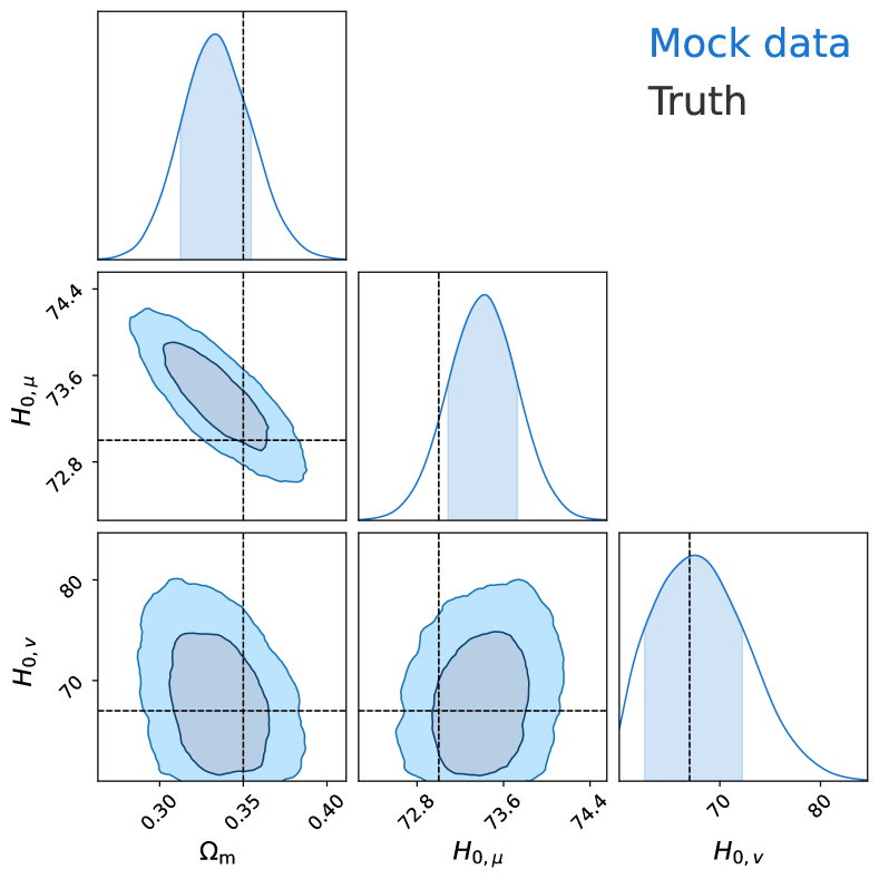
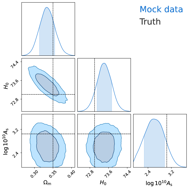
Figure 1: Posterior distribution for the mock test, with the bands indicating the 68% and 95% credible intervals. In the left panel we choose $H_{0,\mu}=73$ km/s/Mpc for the distances and $H_{0,\rm{v}}=67$ km/s/Mpc for the velocity power spectrum; additionally, $\Omega_{\textrm{m}}=0.35$ and $\log_{10}(10^{10}A_{\mathrm{s}})=3.04$. For the analysis in the right panel we assume $H_{0,\mu}=H_{0,\rm{v}}$, but vary $A_{\mathrm{s}}$ which is degenerate with $H_{0,\rm{v}}$. We do not include Cepheids in these mock datasets, and simply set $\delta M\equiv 0$ which leads to an artificially small error in $H_{0,\mu}$. In all figures throughout the paper, $H_{0}$ values are in units of km/s/Mpc.

4.1 Mock dataset

We generate a mock dataset following the steps described in Appendix C. This dataset is modeled with redshifts affected by velocities generated from the velocity covariance matrix in Eq. (2.9), and distance moduli with errors given by $C^{\rm(e)}$ as in Pantheon+. In order to study how well we can recover $H_{0}$ from the peculiar velocities and from the distance moduli, we choose different input values of $H_{0}$ for the velocity covariance, denoted $H_{0,{\rm\rm{v}}}=67$ km/s/Mpc, and the distance modulus, denoted $H_{0,\mu}=73$ km/s/Mpc. As a first step with this mock data, we do not add a velocity dispersion as described in Sec. 2.2, which is present not only in real data but also in $N$-body simulations.

When fixing $A_{\mathrm{s}}$, we can recover both $H_{0,\rm{v}}$ and $H_{0,\mu}$ within $1\sigma$, as we show in the left panel of Fig. 1. In the right-hand side plot of Fig. 1, using the same dataset, we assume just one physical value of $H_{0}=H_{0,\mu}=H_{0,\rm{v}}$: since the velocity covariance was generated with a different value of $H_{0}$ this reproduces now a smaller value of $A_{\mathrm{s}}$ with an only very little increase in goodness of fit ($\log\mathcal{L}=523$ vs 521). As expected within linear perturbation theory, the result mainly depends on $H^{2}_{0}A_{\mathrm{s}}$ and a 10% increase in $H_{0}$ can be compensated with an about 20% decrease in $A_{\mathrm{s}}$. We also see that mapping the redshift error onto the magnitude error does not induce a bias in the analysis of the mock dataset, although for larger datasets a more involved analysis may be necessary [45].

4.2 $N$-body simulation

As a more realistic test dataset, we use a subset of the simulated distances created by the relativistic $N$-body code gevolution [46] to study the impact of cosmic structure on the Hubble diagram in Ref. [47]. For this, a relativistic ray-tracing through the simulation volume has been performed. The simulation covers a cosmological volume of $(2.4\ {\rm Gpc}/h)^{3}$, the metric is sampled on a regular grid of $7680^{3}$ points and the matter density is followed by $7680^{3}$ mass elements. The simulation assumes a flat $\Lambda$CDM cosmology with $H_{0}=67.556$ km/s/Mpc, $\Omega_{\textrm{m}}=0.312046$ and $A_{\mathrm{s}}=2.215\times 10^{-9}$, corresponding to $\log 10^{10}A_{\mathrm{s}}=3.098$. The lightcone was recorded on a circular pencil beam covering $450\ {\rm deg}^{2}$. More details can be found in Ref. [47].

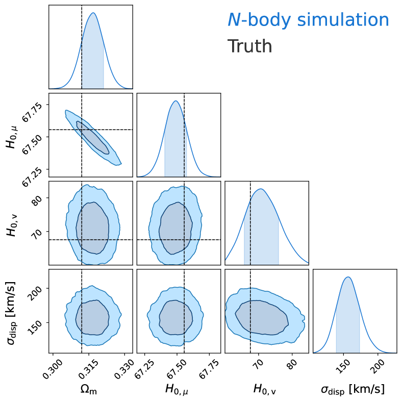
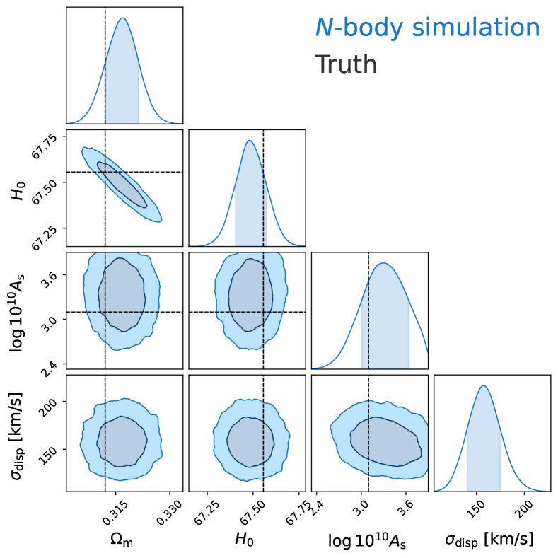
Figure 2: Results from the $N$-body simulation run with gevolution. The blue contours indicate the 68% and 95% credible intervals, while the black dashed lines represent the input cosmological parameters for the $N$-body simulation. The left panel shows that, given $A_{\textrm{s}}$, we can determine $H_{0}$ either via the distance moduli, $H_{0,\mu}$ or via the peculiar velocity covariance, $H_{0,\rm{v}}$. In the right panel, we consider only one value of $H_{0}=H_{0,\mu}=H_{0,\rm{v}}$, and we use the velocity covariance to determine $A_{\textrm{s}}$.

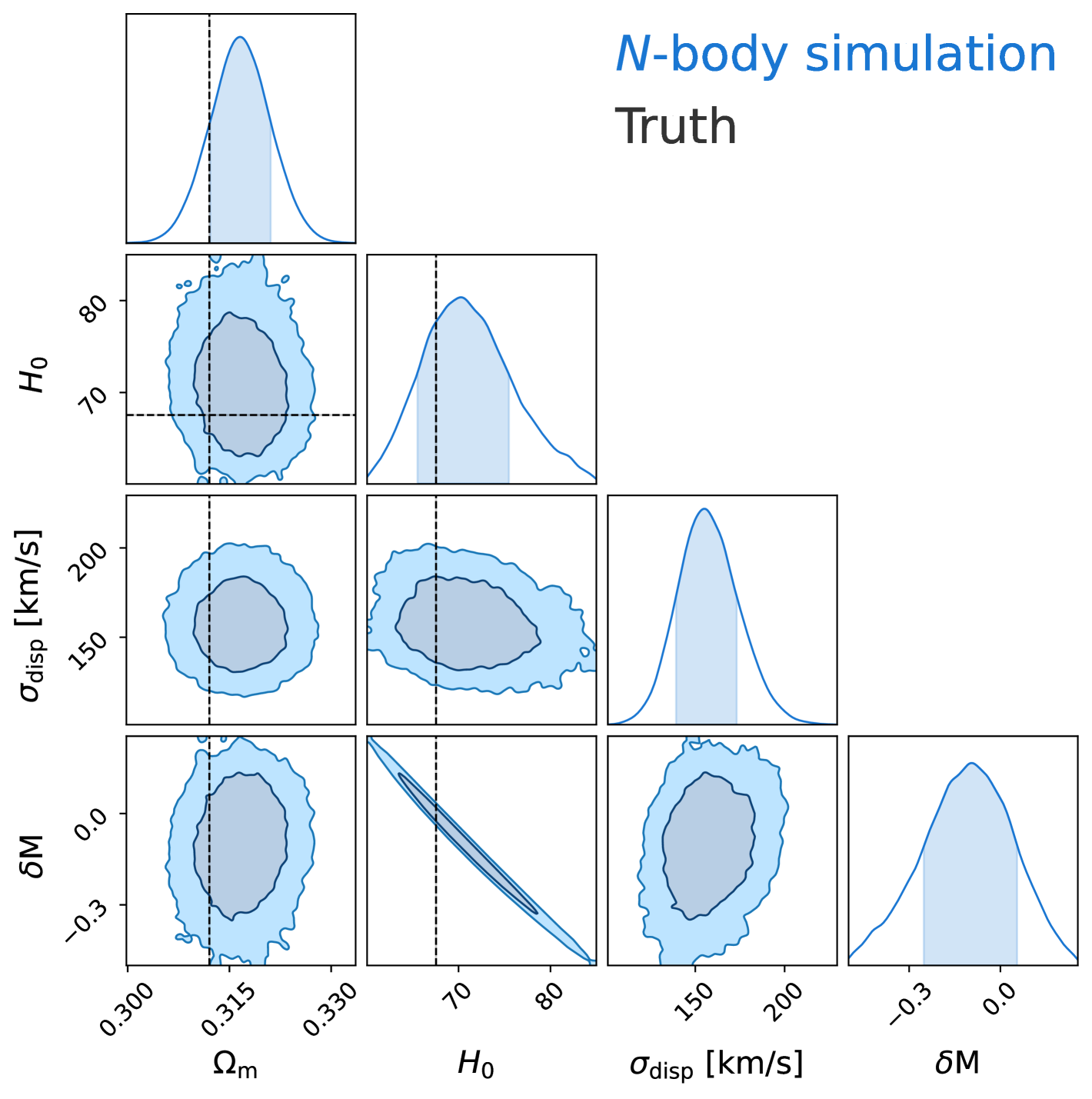
Figure 3: Results from the $N$-body simulation gevolution ‘without cepheids’, namely with $\delta$M acting as calibration parameter. The blue contours indicate the 68% and 95% credible intervals, while the input cosmological parameters for the $N$-body simulation are shown as dashed lines. Fixing $A_{\textrm{s}}$ to the input value, we use the velocity covariance to determine $H_{0}$ without the help of anchors. The degeneracy with $\delta M$, while not being completely lifted, is significantly reduced.

These $N$-body distances contain the velocity and lensing contributions by construction, but have essentially vanishing intrinsic scatter. To make them more realistic, we add random noise to the data with a given constant standard deviation $\sigma_{0}=0.03$, roughly corresponding to one order of magnitude less than Pantheon+. We then write the error covariance matrix as:

$$C^{\rm(e)}_{mn}=\left(\sigma_{0}^{2}+\sigma_{l}^{2}z^{2}\right)\delta_{mn}$$

for the chosen value of $\sigma_{0}$ and for a lensing contribution of $\sigma_{l}=0.055$ [48]. To this we add the velocity covariance $C^{\rm(v)}_{mn}$ and the velocity dispersion $C_{mn}^{\rm(v),disp}$ as described in Sec. 2.

From the large number of distances to halos available in this data set, we randomly select 1701 halos in the redshift range $\left[0.01,1\right]$ with a redshift distribution similar to the one of the Pantheon+ data. Given the box size and resolution, we expect that the large-scale structure is correctly resolved down to significantly smaller redshifts. We also have checked that the monopole, dipole and quadrupole contributions to the luminosity distance are negligible in this near ‘pencil beam’ data.

We perform the same analyses with the $N$-body simulations as in the next section for the real supernova data. We first fix $A_{\textrm{s}}$ and assume two different values of $H_{0}$, one for the distance modulus, $H_{0,\mu}$, and one for the peculiar velocities, $H_{0,{\rm v}}$. The results, shown in the left panel of Fig. 2, indicate that we manage to recover $\Omega_{\textrm{m}}$ and both $H_{0}$ values within 1$\sigma$, with a velocity dispersion of $\sigma_{\rm{disp}}=157\pm 17$ km/s. In the right panel of Fig. 2 we further show that, assuming a single $H_{0}$, we also retrieve the correct value of $\log 10^{10}A_{\textrm{s}}$, with a consistent value of $\sigma_{\rm{disp}}$.

In Fig. 3 we show the results of a parameter estimation mimicking an analysis without any Cepheid anchors. Clearly, the degeneracy between $H_{0}$ and the distance shift $\delta M$ is considerable, but it is partially broken by the velocity covariance, allowing us to recover well the input value of $H_{0}$, for which we find $H_{0}=70.5^{+5.0}_{-4.9}\ \rm{km/s/Mpc}$. The input $\Omega_{\textrm{m}}$ is also well recovered, while the required velocity dispersion of $\sigma_{\rm disp}=155^{+18}_{-16}$ km/s is in good agreement with the Pantheon+ data results discussed below. While the non-linear corrections in the velocity covariance matrix can in principle break the degeneracy between $A_{\textrm{s}}$ and $H_{0}$, we still find in this analysis a strong degeneracy, namely we can either determine $H_{0}$ or $A_{\textrm{s}}$, but not both at the same time. This might be due to the fact that there are very few nearby supernovae in this dataset, so that the non-linear corrections to the velocity covariance are not very important here. We will however always show results including the non-linear modeling of the velocity covariance.

4.3 Pantheon+ data

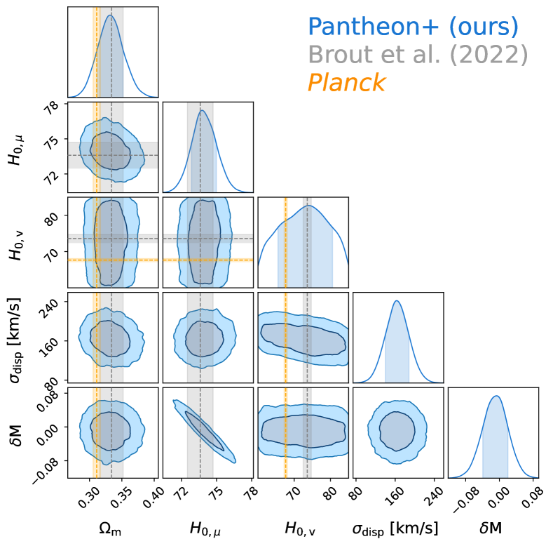
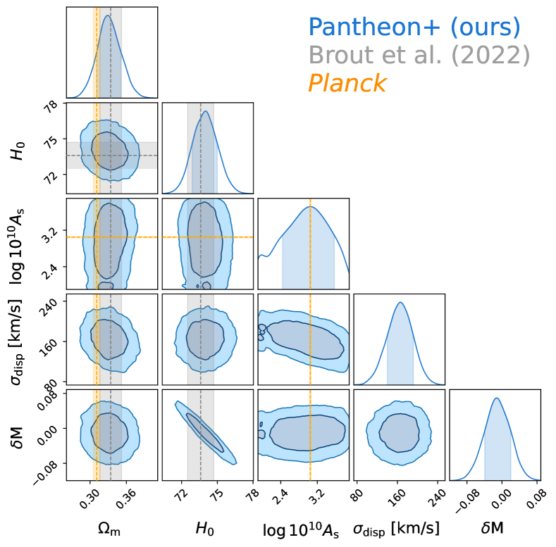
Figure 4: 68% and 95% posterior contours from the Pantheon+ data including Cepheid information. In the left panel, we model the peculiar velocities with fixed $(A_{\textrm{s}},~n_{\textrm{s}})$ from the Planck data, and fit $H_{0}$ from the distance moduli ($H_{0,\mu}$) and from the velocity covariance ($H_{0,\rm{v}}$) independently. The inferred value for $H_{0,\rm{v}}$ has large error bars and cannot distinguish between the value inferred from the traditional supernova analysis (gray bands) and the Planck value (orange bands). In the right panel, we model the data with one value for $H_{0}$ and use the velocity covariance to determine $A_{\textrm{s}}$. Again, the errors are still rather large with present data, but demonstrate the potential of our approach.

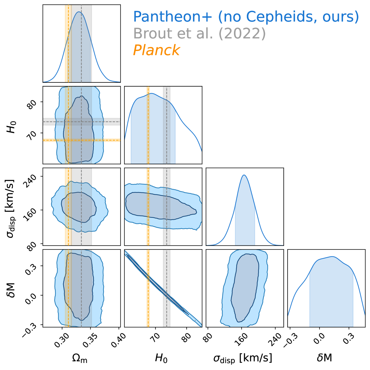
Figure 5: 68% and 95% posterior contours from the Pantheon+ analysis without using Cepheid anchors. The degeneracy between $\delta M$ and $H_{0}$ is broken only by our treatment of the velocity covariance. The Planck values for $H_{0}$ and $\Omega_{\textrm{m}}$ are indicated as orange bands, while in gray we report the values from the latest Pantheon+ analysis [4].

As in our previous analyses (see Refs. [49, 23, 50]), we use the Pantheon+SH0ES dataset providing 1701 lightcurves [4, 21]; of these, 77 SNIa are in galaxies hosting Cepheids, whose absolute distance modulus $\mu_{\mathrm{ceph}}$ is known. For the analysis of the Pantheon+ data, we start from the Pantheon+ covariance matrix with the statistical and systematic contributions from peculiar velocities subtracted, and we add our peculiar velocity covariance matrix $C^{\text{(v)}}_{mn}$. When fixing $A_{\textrm{s}}$ and $n_{\textrm{s}}$ to the Planck values, the velocity covariance matrix depends on $H_{0}$ and $\Omega_{\textrm{m}}$ via the power spectrum $P_{\textrm{v}}$. We first fix $A_{\mathrm{s}}$ to the Planck value and allow for an independent $H_{0}$ for both the distance modulus, $H_{0,\mu}$ and the velocity covariance, $H_{0,\rm{v}}$; the result is shown in the left panel of Fig. 4. Clearly, $H_{0,\rm{v}}$ has very wide contours and cannot distinguish between the values preferred by the distance Pantheon+ data [4] (gray bands) and the Planck data [31] (orange bands). On the other hand, we can use the distance moduli and the velocity covariance to jointly model the value of $H_{0}$, $\Omega_{\textrm{m}}$ and $A_{\textrm{s}}$, which we show in the right panel of Fig. 4. In this way, supernovae provide an independent value of the scalar perturbation amplitude $A_{\textrm{s}}$ which is nearly independent of Planck data (only the value $n_{\textrm{s}}$ is adopted from Planck).

We finally remove the calibrators from the Pantheon+ dataset and perform an analysis assuming a single $H_{0}$ while fixing $A_{\mathrm{s}}$ to its Planck value. The results, presented in Fig. 5, cannot yet distinguish between the Planck value and the value from the standard SNIa analysis; however, we start breaking the degeneracy between $H_{0}$ and $\delta$M, finding:

$$H_{0}=68.7^{+7.7}_{-6.5}\ {\rm km/s/Mpc}\,.$$

All numerical results for our Pantheon+ analyses are presented in Table 2.

Table 2: Parameter constraints (maximum a posteriori $\pm$ 68% credible intervals) for the Pantheon+ analyses, with all details available in Sec. 4.3. All analyses find $\Omega_{{\rm m}}=0.33\pm 0.02$. We have $H_{0,\mu}=H_{0}$ in the second and third rows.

	$H_{0,\mu}$	$H_{0,\rm{v}}$	$\log 10^{10}A_{\mathrm{s}}$	$\sigma_{\rm disp}$	$\delta$M
Analysis	[km/s/Mpc]	[km/s/Mpc]		[km/s]
With Cepheids, free $A_{\mathrm{s}}$ (Fig. 4)	$74.0^{+1.0}_{-1.1}$	-	$3.1^{+0.5}_{-0.6}$	$166^{+26}_{-26}$	$-0.01^{+0.03}_{-0.03}$
With Cepheids, fixed $A_{\mathrm{s}}$ (Fig. 4)	$73.7^{+1.2}_{-0.9}$	$74.0^{+6.5}_{-8.5}$	-	$163^{+25}_{-23}$	$-0.01^{+0.03}_{-0.03}$
No Cepheids, fixed $A_{\mathrm{s}}$ (Fig. 5)	$68.7^{+7.7}_{-6.5}$	-	-	$166^{+25}_{-21}$	$0.13^{+0.21}_{-0.23}$

5 Conclusions

In this paper, we introduce a novel method to use SNIa peculiar velocities to constrain cosmological parameters without the need for anchors such as the Cepheids, by exploiting the $H_{0}$ dependence of the covariance matrix of the peculiar velocities. So far, our analysis constrains either $A_{\mathrm{s}}$ or the Hubble parameter in the velocity power spectrum, $H_{0,\rm{v}}$, since the linear velocity power spectrum only depends on the product $H_{0}^{2}A_{\mathrm{s}}$. With more low redshift supernovae, we shall also become more sensitive to non-linear corrections which break this degeneracy. We developed an efficient differentiable pipeline and validated our approach on mock datasets and on $N$-body simulations. We then applied it to the Pantheon+ data, finding that $H_{0,\rm{v}}=74.0^{+6.5}_{-8.5}$ km/s/Mpc for the double $H_{0}$ analysis, while for the single $H_{0}$ analysis without Cepheids we find $H_{0}=68.7^{+7.7}_{-6.5}$ km/s/Mpc.

Our work showcases a new path to address tensions between early and late Universe probes [51]. Presently, there is a considerable debate concerning the use of anchors for supernova measurements [52, 53, 54]; our method is independent of these anchors, depending only on the peculiar velocity power spectrum. While present data does not have sufficiently many low redshift supernova to allow a precise measurement of the velocity power spectrum, the proposed method will achieve its full potential with upcoming surveys like ZTF [16] and the Vera Rubin Legacy Survey of Space and Time (LSST, [55]), providing significantly more data especially at low redshift. As peculiar velocities contribute most to the Hubble diagram at low redshifts, especially in the analysis of ZTF with an order of magnitude more supernovae with redshifts $z<0.1$, our method promises to unlock precise cosmological constraints without relying on anchors.

We plan to extend our analysis in several ways. For instance, we will implement a differentiable version of the low multipoles of the luminosity distance, based on Ref. [23], which will allow us to jointly sample the multipoles and the cosmological parameters. We will also implement other contributions to the peculiar velocities, such as the vorticity power spectrum. Vorticity is usually neglected when modeling velocities; nevertheless, some works (e.g. [56]) have shown that it is an important contribution to the velocity power spectrum at late time, exactly when peculiar velocities become more and more relevant in the Hubble diagram. We will also further evaluate the robustness of our new implementations with more refined $N$-body simulations.

Most importantly, we plan to apply our routine to larger supernova datasets as the LSST and, in particular, the ZTF. The contribution from ZTF will be particularly relevant since it is expected to observe many supernovae at low redshift; for example, the upcoming Data Release 2.5 is anticipated to contain thousands of objects at $z\leq 0.3$ [19]. In order to obtain competitive constraints which can distinguish between the presently advocated values of $H_{0}$, we will need about 10 times more SNIa at low redshift ($z\lesssim 0.1$) than the present dataset; Pantheon+ contains 664 SNIa with $z<0.1$, excluding the 77 SNIa in galaxies hosting Cepheids. Our approach can also be modified to work with other distance relations like the Tully-Fisher relation [57] and the Fundamental Plane relation [58, 59], as well as to be applied to datasets like CosmicFlows-4 [60], containing distances to 55,877 galaxies collected into 38,065 groups.

6 Data availability

The Pantheon+ dataset and distance modulus covariances are available in the official repository https://github.com/PantheonPlusSH0ES/DataRelease. The data and the code to reproduce our analysis, together with the emulator for the velocity covariance power spectrum, will be made public upon acceptance of this paper at this GitHub repository:
https://github.com/dpiras/veloce github.

Appendix A Derivation of $\delta z$

We assume that the shift in $\bar{z}=z+\delta z_{i}$ due to the peculiar velocity of supernova $i$ is small, so that we can write:

$$\mu(\bar{z})=\mu(z)+\mu^{\prime}(z)\delta z_{i}\,,\quad\delta z_{i}=\frac{v_{i}/c}{1+z_{i}}\,,$$ (A.1)

where $v_{i}={\mathbf{v}}({\mathbf{n}}_{i},z_{i})\cdot{\mathbf{n}}_{i}$ is the radial peculiar velocity of supernova $i$, and ${\mathbf{n}}_{i}$ its position. The derivative of the distance modulus $\mu=5\log_{10}(d_{\mathrm{L}}/1{\rm Mpc})+25$ is given by

$$\mu^{\prime}(z)=\frac{\partial\mu}{\partial z}=\frac{5}{\log(10)}\frac{d_{\mathrm{L}}^{\prime}(z)}{d_{\mathrm{L}}(z)}\,.$$ (A.2)

We can invert the relation to obtain the shift in $z$:

$$\delta z_{i}=\frac{\mu(\bar{z_{i}})-\mu(z_{i})}{\mu^{\prime}(z_{i})}=\frac{\log(10)}{5}\frac{d_{\mathrm{L}}(z_{i})}{d_{\mathrm{L}}^{\prime}(z_{i})}\left[\mu(\bar{z_{i}})-\mu(z_{i})\right]\,.$$ (A.3)

From the definition of the background $d_{\mathrm{L}}(z)$ we have that:

$$\frac{d_{\mathrm{L}}^{\prime}}{d_{\mathrm{L}}}=\frac{1}{1+z}+\frac{1+z}{H(z)d_{\mathrm{L}}(z)}=\frac{1}{1+z}\left(1+\frac{(1+z)^{2}}{H(z)d_{\mathrm{L}}(z)}\right)\,.$$ (A.4)

Furthermore, also $d_{\mathrm{L}}(\bar{z})$ is proportional to the source frequency squared, adding a term $-2\delta z/(1+z)d_{\mathrm{L}}$ which inverts the sign of the first term in the final expression (see Ref. [22] for a detailed derivation including also the gravitational terms). Using the peculiar velocity term of Ref. [22] in the equation for $\delta z$ and writing $\delta\mu^{(v)}=\mu(\bar{z})-\mu(z)$, we find:

$$\delta z_{i} = \frac{\log(10)}{5}\delta\mu^{(v)}_{i}\frac{1+z_{i}}{\frac{c(1+z_{i})^{2}}{H(z_{i})d_{\mathrm{L}}(z_{i})}-1}\,,$$ (A.5)

or equivalently

$$v_{i} = \frac{\log(10)}{5}\delta\mu^{(v)}_{i}\frac{c}{\frac{c(1+z_{i})^{2}}{H(z_{i})d_{\mathrm{L}}(z_{i})}-1}\,,$$ (A.6)

which agrees with Eq. (2.8).

Appendix B Derivation of the window function

To calculate the window function as in Eq. (2.12), we must determine the integrals:

$$W_{mn}(k) = \sum_{i,j=1}^{3}{\mathbf{n}}_{m,i}{\mathbf{n}}_{n,j}\int\frac{\mathrm{d}\Omega_{\hat{k}}}{4\pi}\hat{{\mathbf{k}}}_{i}\,\hat{{\mathbf{k}}}_{j}e^{ik\hat{\mathbf{k}}\cdot(\mathbf{r}_{m}-\mathbf{r}_{n})}\,=\sum_{ij}{\mathbf{n}}_{m,i}{\mathbf{n}}_{n,j}W_{mnij}(k)\,,$$ (B.1)

where ${\mathbf{n}}_{m}={\mathbf{r}}_{m}/r_{m}$ and ${\mathbf{n}}_{n}={\mathbf{r}}_{n}/r_{n}$ are the directions of the $m$-th and $n$-th SNIa respectively. To simplify the calculation we orient the coordinate system in ${\mathbf{k}}$-space such that $\mathbf{r}_{m}-\mathbf{r}_{n}$ is in the $z$-direction, and both $\mathbf{r}_{m}$ and $\mathbf{r}_{n}$ are in the $\varphi=0$ plane; hence $r_{m2}=r_{n2}=0$. Furthermore, it is easy to see that the $\varphi$-integral of $W_{mnij}(k)$ vanishes whenever $i\neq j$. Using $\cos\theta=\mu$ such that $\mathrm{d}\Omega_{\hat{k}}=\sin\theta d\theta d\varphi=d\mu d\varphi$ and setting $|{\mathbf{r}_{m}-\mathbf{r}_{n}}|=R_{mn}$, we obtain:

$$W_{mn33}(k) = \frac{1}{2}\int_{-1}^{1}\mu^{2}e^{ikR_{mn}\mu}$$ (B.2)

$$= \frac{2kR_{mn}\cos(kR_{mn})+((kR_{mn})^{2}-2)\sin(kR_{mn})}{(kR_{mn})^{3}}\,,$$

$$W_{mn11}(k) = \frac{1}{4\pi}\int_{0}^{2\pi}\cos^{2}\varphi\int_{-1}^{1}(1-\mu^{2})e^{ikR_{mn}\mu}$$ (B.3)

$$= \frac{-2kR_{mn}\cos(kR_{mn})+2\sin(kR_{mn})}{(kR_{mn})^{3}}\,.$$

We now use that:

$$W_{mn}(k)=(n_{m3}n_{n3}+n_{m1}n_{n1})W_{mn33}+n_{m1}n_{n1}(W_{mn11}-W_{mn33})\,.$$

Furthermore, one easily verifies that:

$$W_{mn33}(k)=\frac{1}{3}(j_{0}(kR_{mn})-2j_{2}(kR_{mn}))$$

and

$$W_{mn11}(k)-W_{mn33}(k)=j_{2}(kR_{mn})\,.$$

We use also that:

$$n_{m3}n_{n3}+n_{m1}n_{m1}=\cos\alpha_{mn}\,,$$

and the elementary triangle relation

$$\frac{\sin\theta_{m}}{r_{n}}=\frac{\sin\theta_{n}}{r_{m}}=\frac{\sin\alpha_{mn}}{R_{mn}}\,,$$

which implies

$$n_{m1}=\sin\theta_{m}=r_{n}\frac{\sin\alpha_{mn}}{R_{mn}}$$

and

$$n_{n1}=\sin\theta_{n}=r_{m}\frac{\sin\alpha_{mn}}{R_{mn}}\,.$$

Putting it all together we arrive at the final result:

$$W_{mn}(k)= \frac{1}{3}\cos{\alpha_{mn}}(j_{0}(kR_{mn})-2j_{2}(kR_{mn}))+\frac{r_{m}r_{n}}{R_{mn}^{2}}j_{2}(kR_{mn})\sin^{2}{\alpha_{mn}}\,.$$ (B.4)

Appendix C Mock dataset

For the sake of simplicity and to avoid numerical instabilities, we create our mock dataset starting from a subset of Pantheon+ containing 1106 individual lightcurves with heliocentric redshift differences larger than $5\times 10^{-5}$. Consequently, we also subsample the error covariance $C^{\rm(e)}_{mn}$ obtained from the full Pantheon+ covariance; we keep only the row and column corresponding to the first occurring SNIa when selecting the unique elements.

We choose the heliocentric redshifts of the original dataset as background redshift $\bar{z}$ of the mock dataset. We then define the mock observed redshifts $z^{\rm mock}_{i}$ for the $i$-th object as:

$$z^{\rm mock}_{i}=\bar{z}_{i}+\delta z_{i}\,,$$ (C.1)

with the peculiar velocity contribution

$$\delta z_{i}=\sum_{j}D_{ij}g_{j}\,.$$ (C.2)

Here, $g_{j}$ is sampled from a Gaussian distribution with mean 0 and variance $1$, while $D_{ij}$ is obtained from the Cholesky decomposition of our velocity covariance:

$$\frac{C^{\rm(v),z}}{c^{2}}=DD^{\rm T},$$ (C.3)

with $c$ being the speed of light and

$$C^{\rm(v),z}=C^{\rm(v),v}(1+z_{m})(1+z_{n}).$$ (C.4)

$C^{\rm(v),v}$ is the covariance in Eq. (2.9) obtained assuming $H_{0,\rm{v}}=67$ km/s/Mpc, $\Omega_{\textrm{m}}=0.35$ and $\log_{10}(10^{10}A_{\mathrm{s}})=3.04$. Finally, we define the mock distance modulus as:

$$\mu_{i}^{\rm mock}=\mu_{i}(\bar{z}_{i})+h_{i}\,\sigma^{\mu}_{i}$$ (C.5)

with $h_{i}$ sampled from a Gaussian distribution with mean 0 and variance 1, and $(\sigma^{\mu}_{i})^{2}$ is the $i$-th element of the diagonal of the Pantheon+ covariance without peculiar velocity correction. $\mu_{i}(\bar{z}_{i})$ is obtained from Eq. (2.3) assuming the same cosmology as for $z^{\rm mock}_{i}$ except for $H_{0,\mu}=73$ km/s/Mpc.

References

- [1] B. P. Schmidt, N. B. Suntzeff, M. M. Phillips, R. A. Schommer, A. Clocchiatti, R. P. Kirshner, P. Garnavich, P. Challis, B. Leibundgut, J. Spyromilio, A. G. Riess, A. V. Filippenko, M. Hamuy, R. C. Smith, C. Hogan, C. Stubbs, A. Diercks, D. Reiss, R. Gilliland, J. Tonry, J. Maza, A. Dressler, J. Walsh, and R. Ciardullo, The High-Z Supernova Search: Measuring Cosmic Deceleration and Global Curvature of the Universe Using Type IA Supernovae, ApJ 507 (Nov., 1998) 46–63, [astro-ph/9805200].
- [2] A. G. Riess, A. V. Filippenko, P. Challis, A. Clocchiatti, A. Diercks, P. M. Garnavich, R. L. Gilliland, C. J. Hogan, S. Jha, R. P. Kirshner, B. Leibundgut, M. M. Phillips, D. Reiss, B. P. Schmidt, R. A. Schommer, R. C. Smith, J. Spyromilio, C. Stubbs, N. B. Suntzeff, and J. Tonry, Observational Evidence from Supernovae for an Accelerating Universe and a Cosmological Constant, AJ 116 (Sept., 1998) 1009–1038, [astro-ph/9805201].
- [3] S. Perlmutter, G. Aldering, G. Goldhaber, R. A. Knop, P. Nugent, P. G. Castro, S. Deustua, S. Fabbro, A. Goobar, D. E. Groom, I. M. Hook, A. G. Kim, M. Y. Kim, J. C. Lee, N. J. Nunes, R. Pain, C. R. Pennypacker, R. Quimby, C. Lidman, R. S. Ellis, M. Irwin, R. G. McMahon, P. Ruiz-Lapuente, N. Walton, B. Schaefer, B. J. Boyle, A. V. Filippenko, T. Matheson, A. S. Fruchter, N. Panagia, H. J. M. Newberg, and W. J. Couch, Measurements of and from 42 High-Redshift Supernovae, ApJ 517 (June, 1999) 565–586, [astro-ph/9812133].
- [4] D. Brout, D. Scolnic, B. Popovic, A. G. Riess, A. Carr, J. Zuntz, R. Kessler, T. M. Davis, S. Hinton, D. Jones, W. D. Kenworthy, E. R. Peterson, K. Said, G. Taylor, N. Ali, P. Armstrong, P. Charvu, A. Dwomoh, C. Meldorf, A. Palmese, H. Qu, B. M. Rose, B. Sanchez, C. W. Stubbs, M. Vincenzi, C. M. Wood, P. J. Brown, R. Chen, K. Chambers, D. A. Coulter, M. Dai, G. Dimitriadis, A. V. Filippenko, R. J. Foley, S. W. Jha, L. Kelsey, R. P. Kirshner, A. Möller, J. Muir, S. Nadathur, Y.-C. Pan, A. Rest, C. Rojas-Bravo, M. Sako, M. R. Siebert, M. Smith, B. E. Stahl, and P. Wiseman, The Pantheon+ Analysis: Cosmological Constraints, The Astrophysical Journal 938 (oct, 2022) 110.
- [5] A. Carr, T. M. Davis, D. Scolnic, K. Said, D. Brout, E. R. Peterson, and R. Kessler, The Pantheon+ analysis: Improving the redshifts and peculiar velocities of Type Ia supernovae used in cosmological analyses, Publications of the Astronomical Society of Australia 39 (2022).
- [6] T. M. Davis, L. Hui, J. A. Frieman, T. Haugbølle, R. Kessler, B. Sinclair, J. Sollerman, B. Bassett, J. Marriner, E. Mörtsell, R. C. Nichol, M. W. Richmond, M. Sako, D. P. Schneider, and M. Smith, The Effect of Peculiar Velocities on Supernova Cosmology, ApJ 741 (Nov., 2011) 67, [arXiv:1012.2912].
- [7] G. Efstathiou, To H0 or not to H0?, Mon. Not. Roy. Astron. Soc. 505 (2021), no. 3 3866–3872, [arXiv:2103.08723].
- [8] A. G. Riess et al., A Comprehensive Measurement of the Local Value of the Hubble Constant with 1 km s-1 Mpc-1 Uncertainty from the Hubble Space Telescope and the SH0ES Team, Astrophys. J. Lett. 934 (2022), no. 1 L7, [arXiv:2112.04510].
- [9] E. Macaulay, H. A. Feldman, P. G. Ferreira, A. H. Jaffe, S. Agarwal, M. J. Hudson, and R. Watkins, Power spectrum estimation from peculiar velocity catalogues, MNRAS 425 (Sept., 2012) 1709–1717, [arXiv:1111.3338].
- [10] H. A. Feldman, R. Watkins, and M. J. Hudson, Cosmic flows on 100 h-1 Mpc scales: standardized minimum variance bulk flow, shear and octupole moments, MNRAS 407 (Oct., 2010) 2328–2338, [arXiv:0911.5516].
- [11] A. Johnson, C. Blake, J. Koda, Y.-Z. Ma, M. Colless, M. Crocce, T. M. Davis, H. Jones, C. Magoulas, J. R. Lucey, J. Mould, M. I. Scrimgeour, and C. M. Springob, The 6dF Galaxy Survey: cosmological constraints from the velocity power spectrum, MNRAS 444 (Nov., 2014) 3926–3947, [arXiv:1404.3799].
- [12] L. A. Campbell et al., The 6dF Galaxy Survey: Fundamental Plane Data, Mon. Not. Roy. Astron. Soc. 443 (2014), no. 2 1231–1251, [arXiv:1406.4867].
- [13] C. Howlett, L. Staveley-Smith, P. J. Elahi, T. Hong, T. H. Jarrett, D. H. Jones, B. S. Koribalski, L. M. Macri, K. L. Masters, and C. M. Springob, 2MTF – VI. Measuring the velocity power spectrum, Mon. Not. Roy. Astron. Soc. 471 (2017), no. 3 3135–3151, [arXiv:1706.05130].
- [14] K. L. Masters, C. M. Springob, and J. P. Huchra, 2MTF. I. The Tully-Fisher Relation in the Two Micron All Sky Survey J, H, and K Bands, AJ 135 (May, 2008) 1738–1748, [arXiv:0711.4305].
- [15] B. Carreres et al., Growth-rate measurement with type-Ia supernovae using ZTF survey simulations, Astron. Astrophys. 674 (2023) A197, [arXiv:2303.01198].
- [16] E. C. Bellm, S. R. Kulkarni, M. J. Graham, R. Dekany, R. M. Smith, R. Riddle, F. J. Masci, G. Helou, T. A. Prince, S. M. Adams, C. Barbarino, T. Barlow, J. Bauer, R. Beck, J. Belicki, R. Biswas, N. Blagorodnova, D. Bodewits, B. Bolin, V. Brinnel, T. Brooke, B. Bue, M. Bulla, R. Burruss, S. B. Cenko, C.-K. Chang, A. Connolly, M. Coughlin, J. Cromer, V. Cunningham, K. De, A. Delacroix, V. Desai, D. A. Duev, G. Eadie, T. L. Farnham, M. Feeney, U. Feindt, D. Flynn, A. Franckowiak, S. Frederick, C. Fremling, A. Gal-Yam, S. Gezari, M. Giomi, D. A. Goldstein, V. Z. Golkhou, A. Goobar, S. Groom, E. Hacopians, D. Hale, J. Henning, A. Y. Q. Ho, D. Hover, J. Howell, T. Hung, D. Huppenkothen, D. Imel, W.-H. Ip, Ž. Ivezić, E. Jackson, L. Jones, M. Juric, M. M. Kasliwal, S. Kaspi, S. Kaye, M. S. P. Kelley, M. Kowalski, E. Kramer, T. Kupfer, W. Landry, R. R. Laher, C.-D. Lee, H. W. Lin, Z.-Y. Lin, R. Lunnan, M. Giomi, A. Mahabal, P. Mao, A. A. Miller, S. Monkewitz, P. Murphy, C.-C. Ngeow, J. Nordin, P. Nugent, E. Ofek, M. T. Patterson, B. Penprase, M. Porter, L. Rauch, U. Rebbapragada, D. Reiley, M. Rigault, H. Rodriguez, J. v. Roestel, B. Rusholme, J. v. Santen, S. Schulze, D. L. Shupe, L. P. Singer, M. T. Soumagnac, R. Stein, J. Surace, J. Sollerman, P. Szkody, F. Taddia, S. Terek, A. Van Sistine, S. van Velzen, W. T. Vestrand, R. Walters, C. Ward, Q.-Z. Ye, P.-C. Yu, L. Yan, and J. Zolkower, The Zwicky Transient Facility: System Overview, Performance, and First Results, Publications of the Astronomical Society of the Pacific 131 (dec, 2018) 018002.
- [17] C. Ravoux et al., Generalized framework for likelihood-based field-level inference of growth rate from velocity and density fields, arXiv:2501.16852.
- [18] B. Carreres et al., ZTF SN Ia DR2: Peculiar velocities’ impact on the Hubble diagram, Astron. Astrophys. 694 (2025) A8, [arXiv:2405.20409].
- [19] M. Rigault et al., ZTF SN Ia DR2: Overview, Astron. Astrophys. 694 (2025) A1, [arXiv:2409.04346].
- [20] A. Abate and O. Lahav, The Three Faces of Omega: Testing Gravity with Low and High Redshift SN Ia Surveys, Mon. Not. Roy. Astron. Soc. 389 (2008) 47, [arXiv:0805.3160].
- [21] D. Scolnic, D. Brout, A. Carr, A. G. Riess, T. M. Davis, A. Dwomoh, D. O. Jones, N. Ali, P. Charvu, R. Chen, E. R. Peterson, B. Popovic, B. M. Rose, C. M. Wood, P. J. Brown, K. Chambers, D. A. Coulter, K. G. Dettman, G. Dimitriadis, A. V. Filippenko, R. J. Foley, S. W. Jha, C. D. Kilpatrick, R. P. Kirshner, Y.-C. Pan, A. Rest, C. Rojas-Bravo, M. R. Siebert, B. E. Stahl, and W. Zheng, The Pantheon+ Analysis: The Full Data Set and Light-curve Release, ApJ 938 (Oct., 2022) 113, [arXiv:2112.03863].
- [22] C. Bonvin, R. Durrer, and M. A. Gasparini, Fluctuations of the luminosity distance, Phys. Rev. D 73 (2006) 023523, [astro-ph/0511183]. [Erratum: Phys.Rev.D 85, 029901 (2012)].
- [23] F. Sorrenti, R. Durrer, and M. Kunz, The low multipoles in the Pantheon+SH0ES data, JCAP 04 (2025) 013, [arXiv:2403.17741].
- [24] Y.-Z. Ma, C. Gordon, and H. A. Feldman, Peculiar velocity field: Constraining the tilt of the Universe, Phys. Rev. D 83 (May, 2011) 103002.
- [25] Euclid Collaboration, G. Jelic-Cizmek et al., Euclid preparation - XL. Impact of magnification on spectroscopic galaxy clustering, Astron. Astrophys. 685 (2024) A167, [arXiv:2311.03168].
- [26] M. Abramowitz and I. Stegun, Handbook of Mathematical Functions. Dover Publications, New York, 1972.
- [27] N. E. Chisari and A. Pontzen, Unequal time correlators and the Zel’dovich approximation, Phys. Rev. D 100 (Jul, 2019) 023543.
- [28] A. Lewis, A. Challinor, and A. Lasenby, Efficient computation of CMB anisotropies in closed FRW models, Astrophys. J. 538 (2000) 473–476, [astro-ph/9911177].
- [29] J. Koda, C. Blake, T. Davis, C. Magoulas, C. M. Springob, M. Scrimgeour, A. Johnson, G. B. Poole, and L. Staveley-Smith, Are peculiar velocity surveys competitive as a cosmological probe?, Mon. Not. Roy. Astron. Soc. 445 (2014), no. 4 4267–4286, [arXiv:1312.1022].
- [30] J. Bel, A. Pezzotta, C. Carbone, E. Sefusatti, and L. Guzzo, Accurate fitting functions for peculiar velocity spectra in standard and massive-neutrino cosmologies, Astron. Astrophys. 622 (2019) A109, [arXiv:1809.09338].
- [31] Planck Collaboration, N. Aghanim et al., Planck 2018 results. VI. Cosmological parameters, Astron. Astrophys. 641 (2020) A6, [arXiv:1807.06209]. [Erratum: Astron.Astrophys. 652, C4 (2021)].
- [32] C. Pryor and G. Meylan, Velocity Dispersions for Galactic Globular Clusters, in Structure and Dynamics of Globular Clusters (S. G. Djorgovski and G. Meylan, eds.), vol. 50 of Astronomical Society of the Pacific Conference Series, p. 357, Jan., 1993.
- [33] P. J. Godwin and D. Lynden-Bell, Evidence of a small velocity dispersion for the Carina dwarf spheroidal ?, MNRAS 229 (Nov., 1987) 7P–13.
- [34] A. Spurio Mancini, D. Piras, J. Alsing, B. Joachimi, and M. P. Hobson, CosmoPower: emulating cosmological power spectra for accelerated Bayesian inference from next-generation surveys, Monthly Notices of the Royal Astronomical Society 511 (Jan, 2022) 1771–1788.
- [35] J. D. Talman, Numerical Fourier and Bessel transforms in logarithmic variables, Journal of Computational Physics 29 (1978), no. 1 35–48.
- [36] X. Fang, E. Krause, T. Eifler, and N. MacCrann, Beyond Limber: Efficient computation of angular power spectra for galaxy clustering and weak lensing, JCAP 05 (2020) 010, [arXiv:1911.11947].
- [37] J. Bradbury, R. Frostig, P. Hawkins, M. J. Johnson, C. Leary, D. Maclaurin, G. Necula, A. Paszke, J. VanderPlas, S. Wanderman-Milne, and Q. Zhang, JAX: composable transformations of Python+NumPy programs, 2018.
- [38] R. Frostig, M. Johnson, and C. Leary, Compiling machine learning programs via high-level tracing, in SysML (2018), 2018.
- [39] D. Foreman-Mackey, D. W. Hogg, D. Lang, and J. Goodman, emcee: The MCMC Hammer, Publ. Astron. Soc. Pac. 125 (Mar., 2013) 306, [arXiv:1202.3665].
- [40] J. Goodman and J. Weare, Ensemble samplers with affine invariance, Communications in Applied Mathematics and Computational Science 5 (Jan., 2010) 65–80.
- [41] D. Piras and A. Spurio Mancini, CosmoPower-JAX: high-dimensional Bayesian inference with differentiable cosmological emulators, The Open Journal of Astrophysics 6 (July, 2023) 20, [arXiv:2305.06347].
- [42] G. L. Jones and Q. Qin, Markov Chain Monte Carlo in Practice, Annual Review of Statistics and Its Application 9 (Mar., 2022) 557–578.
- [43] S. R. Hinton, ChainConsumer, The Journal of Open Source Software 1 (Aug., 2016) 00045.
- [44] Planck Collaboration, P. A. R. Ade et al., Planck intermediate results. XVI. Profile likelihoods for cosmological parameters, Astron. Astrophys. 566 (2014) A54, [arXiv:1311.1657].
- [45] M. C. March, R. Trotta, P. Berkes, G. D. Starkman, and P. M. Vaudrevange, Improved constraints on cosmological parameters from SNIa data, Mon. Not. Roy. Astron. Soc. 418 (2011) 2308–2329, [arXiv:1102.3237].
- [46] J. Adamek, D. Daverio, R. Durrer, and M. Kunz, gevolution: a cosmological N-body code based on General Relativity, JCAP 07 (2016) 053, [arXiv:1604.06065].
- [47] J. Adamek, C. Clarkson, L. Coates, R. Durrer, and M. Kunz, Bias and scatter in the Hubble diagram from cosmological large-scale structure, Phys. Rev. D 100 (2019), no. 2 021301, [arXiv:1812.04336].
- [48] J. Jonsson, M. Sullivan, I. Hook, S. Basa, R. Carlberg, A. Conley, D. Fouchez, D. A. Howell, K. Perrett, and C. Pritchet, Constraining dark matter halo properties using lensed SNLS supernovae, Mon. Not. Roy. Astron. Soc. 405 (2010) 535, [arXiv:1002.1374].
- [49] F. Sorrenti, R. Durrer, and M. Kunz, The dipole of the Pantheon+SH0ES data, JCAP 11 (2023) 054, [arXiv:2212.10328].
- [50] F. Sorrenti, R. Durrer, and M. Kunz, A local infall from a cosmographic analysis of Pantheon+, JCAP 12 (2024) 003, [arXiv:2407.07002].
- [51] L. Verde, T. Treu, and A. G. Riess, Tensions between the Early and the Late Universe, Nature Astron. 3 (2019) 891, [arXiv:1907.10625].
- [52] W. L. Freedman, B. F. Madore, I. S. Jang, T. J. Hoyt, A. J. Lee, and K. A. Owens, Status Report on the Chicago-Carnegie Hubble Program (CCHP): Measurement of the Hubble Constant Using the Hubble and James Webb Space Telescopes, arXiv:2408.06153.
- [53] A. G. Riess et al., JWST Validates HST Distance Measurements: Selection of Supernova Subsample Explains Differences in JWST Estimates of Local H 0, Astrophys. J. 977 (2024), no. 1 120, [arXiv:2408.11770].
- [54] W. Freedman, The expanding Universe — do ongoing tensions leave room for new physics?, Nature 639 (2025), no. 8056 858–860.
- [55] LSST Science Collaboration, P. A. Abell, J. Allison, S. F. Anderson, J. R. Andrew, J. R. P. Angel, L. Armus, D. Arnett, S. J. Asztalos, T. S. Axelrod, S. Bailey, D. R. Ballantyne, J. R. Bankert, W. A. Barkhouse, J. D. Barr, L. F. Barrientos, A. J. Barth, J. G. Bartlett, A. C. Becker, J. Becla, T. C. Beers, J. P. Bernstein, R. Biswas, M. R. Blanton, J. S. Bloom, J. J. Bochanski, P. Boeshaar, K. D. Borne, M. Bradac, W. N. Brandt, C. R. Bridge, M. E. Brown, R. J. Brunner, J. S. Bullock, A. J. Burgasser, J. H. Burge, D. L. Burke, P. A. Cargile, S. Chandrasekharan, G. Chartas, S. R. Chesley, Y.-H. Chu, D. Cinabro, M. W. Claire, C. F. Claver, D. Clowe, A. J. Connolly, K. H. Cook, J. Cooke, A. Cooray, K. R. Covey, C. S. Culliton, R. de Jong, W. H. de Vries, V. P. Debattista, F. Delgado, I. P. Dell’Antonio, S. Dhital, R. Di Stefano, M. Dickinson, B. Dilday, S. G. Djorgovski, G. Dobler, C. Donalek, G. Dubois-Felsmann, J. Durech, A. Eliasdottir, M. Eracleous, L. Eyer, E. E. Falco, X. Fan, C. D. Fassnacht, H. C. Ferguson, Y. R. Fernandez, B. D. Fields, D. Finkbeiner, E. E. Figueroa, D. B. Fox, H. Francke, J. S. Frank, J. Frieman, S. Fromenteau, M. Furqan, G. Galaz, A. Gal-Yam, P. Garnavich, E. Gawiser, J. Geary, P. Gee, R. R. Gibson, K. Gilmore, E. A. Grace, R. F. Green, W. J. Gressler, C. J. Grillmair, S. Habib, J. S. Haggerty, M. Hamuy, A. W. Harris, S. L. Hawley, A. F. Heavens, L. Hebb, T. J. Henry, E. Hileman, E. J. Hilton, K. Hoadley, J. B. Holberg, M. J. Holman, S. B. Howell, L. Infante, Z. Ivezic, S. H. Jacoby, B. Jain, R, Jedicke, M. J. Jee, J. Garrett Jernigan, S. W. Jha, K. V. Johnston, R. L. Jones, M. Juric, M. Kaasalainen, Styliani, Kafka, S. M. Kahn, N. A. Kaib, J. Kalirai, J. Kantor, M. M. Kasliwal, C. R. Keeton, R. Kessler, Z. Knezevic, A. Kowalski, V. L. Krabbendam, K. S. Krughoff, S. Kulkarni, S. Kuhlman, M. Lacy, S. Lepine, M. Liang, A. Lien, P. Lira, K. S. Long, S. Lorenz, J. M. Lotz, R. H. Lupton, J. Lutz, L. M. Macri, A. A. Mahabal, R. Mandelbaum, P. Marshall, M. May, P. M. McGehee, B. T. Meadows, A. Meert, A. Milani, C. J. Miller, M. Miller, D. Mills, D. Minniti, D. Monet, A. S. Mukadam, E. Nakar, D. R. Neill, J. A. Newman, S. Nikolaev, M. Nordby, P. O’Connor, M. Oguri, J. Oliver, S. S. Olivier, J. K. Olsen, K. Olsen, E. W. Olszewski, H. Oluseyi, N. D. Padilla, A. Parker, J. Pepper, J. R. Peterson, C. Petry, P. A. Pinto, J. L. Pizagno, B. Popescu, A. Prsa, V. Radcka, M. J. Raddick, A. Rasmussen, A. Rau, J. Rho, J. E. Rhoads, G. T. Richards, S. T. Ridgway, B. E. Robertson, R. Roskar, A. Saha, A. Sarajedini, E. Scannapieco, T. Schalk, R. Schindler, and S. Schmidt, LSST Science Book, Version 2.0, arXiv e-prints (Dec., 2009) arXiv:0912.0201, [arXiv:0912.0201].
- [56] G. Jelic-Cizmek, F. Lepori, J. Adamek, and R. Durrer, The generation of vorticity in cosmological N-body simulations, JCAP 09 (2018) 006, [arXiv:1806.05146].
- [57] R. B. Tully and J. R. Fisher, A New method of determining distances to galaxies, Astron. Astrophys. 54 (1977) 661–673.
- [58] S. Djorgovski and M. Davis, Fundamental properties of elliptical galaxies, Astrophys. J. 313 (1987) 59.
- [59] A. Dressler, D. Lynden-Bell, D. Burstein, R. L. Davies, S. M. Faber, R. Terlevich, and G. Wegner, Spectroscopy and Photometry of Elliptical Galaxies. I. New Distance Estimator, ApJ 313 (Feb., 1987) 42.
- [60] R. B. Tully et al., Cosmicflows-4, Astrophys. J. 944 (2023), no. 1 94, [arXiv:2209.11238].