Theory of zonal flow growth and propagation in toroidal geometry

Abstract

The toroidal geometry of tokamaks and stellarators is known to play a crucial role in the linear physics of zonal flows, leading to e.g. the Rosenbluth-Hinton residual and geodesic acoustic modes. However, descriptions of the nonlinear zonal flow growth from a turbulent background typically resort to simplified models of the geometry. We present a generalised theory of the secondary instability to model the zonal flow growth from turbulent fluctuations in toroidal geometry, demonstrating that the radial magnetic drift substantially affects the nonlinear zonal flow dynamics. In particular, the toroidicity gives rise to a new branch of propagating zonal flows, the toroidal secondary mode, which is nonlinearly supported by the turbulence. We present a theory of this mode and compare the theory against gyrokinetic simulations of the secondary mode. The connection with other secondary modes - the ion-temperature-gradient and Rogers-Dorland-Kotschenreuther secondary modes - is also examined.

1 Introduction

Magnetic confinement fusion is plagued by microinstabilities which cause large turbulent heat fluxes and make it difficult to reach the high temperatures required to sustain thermonuclear fusion. Of all the microinstabilities, the most virulent is typically the ion-temperature-gradient (ITG) mode (Coppi et al., 1967). There is however a silver lining, as ion gyroradius scale modes tend to generate strong zonal flows (ZFs) that shear apart turbulent eddies and reduce the saturation level (Lin et al., 1998; Terry, 2000; Dimits et al., 2000; Rogers et al., 2000). Close to marginality, the ZFs can even lead to a nearly complete suppression of the turbulence, nonlinearly increasing the critical gradient threshold beyond which an appreciable heat flux is observed (Dimits et al., 2000).

The linear physics of ZFs in toroidal geometry describes two separate branches: stationary (zero frequency) ZFs and the fast-oscillating geodesic acoustic modes (GAMs) (Winsor et al., 1968; Conway et al., 2021). Crucially, the radial magnetic drift induced by toroidicity couples ZFs to ‘up-down’ (in a tokamak) asymmetric pressure perturbations through the Stringer-Winsor (SW) force (Winsor et al., 1968; Stringer, 1969; Hassam and Drake, 1993; Hallatschek and Biskamp, 2001). The GAM branch of ZFs stems from this SW force, with the up-down asymmetric pressure originating from the compression and expansion of the ZFs due to toroidicity. Stationary ZFs persist in a torus because they produce fluxes parallel to the magnetic field lines that compensate for the compression and expansion. The stationary ZFs are weakened by toroidicity: for typical initial conditions, ZFs linearly decay to the Rosenbluth-Hinton residual (Rosenbluth and Hinton, 1998; Hinton and Rosenbluth, 1999).

While the linear physics of ZFs in tori is well known, the nonlinear mechanisms for ZF growth and saturation are less well understood. As the ZF advection is within flux surfaces, the ZFs cannot linearly extract free-energy from the background radial gradients and must instead be nonlinearly driven by drift-wave (DW) turbulence.

Most studies of ZF drive have focused on the role of the nonlinear Reynolds and diamagnetic stresses in driving ZFs, generally employing reduced models ignoring the effects of toroidicity. The nonlinear stresses can cause ZF growth through a modulational instability mechanism, whereby a linearly unstable ‘primary’ mode (e.g. an ITG) becomes nonlinearly unstable to ‘secondary’ perturbations. The paradigmatic work of Rogers et al. (2000) employed this secondary mode approach to describe the nonlinear growth of ZFs, leading to a purely growing mode which we call the Rogers-Dorland-Kotschenreuther (RDK) secondary mode in this article. More generally, the ZF drive by nonlinear stresses underlying the RDK secondary mode has been studied e.g. in quasilinear models of the ZF-DW system’s evolution (Diamond et al., 2001; Parker and Krommes, 2013; Zhu and Dodin, 2021), in studies of Z-pinch turbulence (Ivanov et al., 2020, 2022), and through various generalisations to include kinetic effects (Plunk, 2007), a finite DW oscillation frequency (Chen et al., 2000), and variation of the flux surface compression along the magnetic field (Plunk and Navarro, 2017).

Another less studied mechanism for ZF drive hinges on the Stringer-Winsor (SW) force. The up-down asymmetric pressure perturbations can be nonlinearly generated by the DWs, and in turn the SW force produced by these asymmetries will drive ZFs. In previous work, the drive of ZFs by the SW force has been studied with the up-down pressure asymmetry assumed ab initio (Hassam and Drake, 1993; Lee et al., 2023) or it was taken to result from zonal flow shearing in conjunction with magnetic shear (Hallatschek and Biskamp, 2001; Itoh et al., 2005).

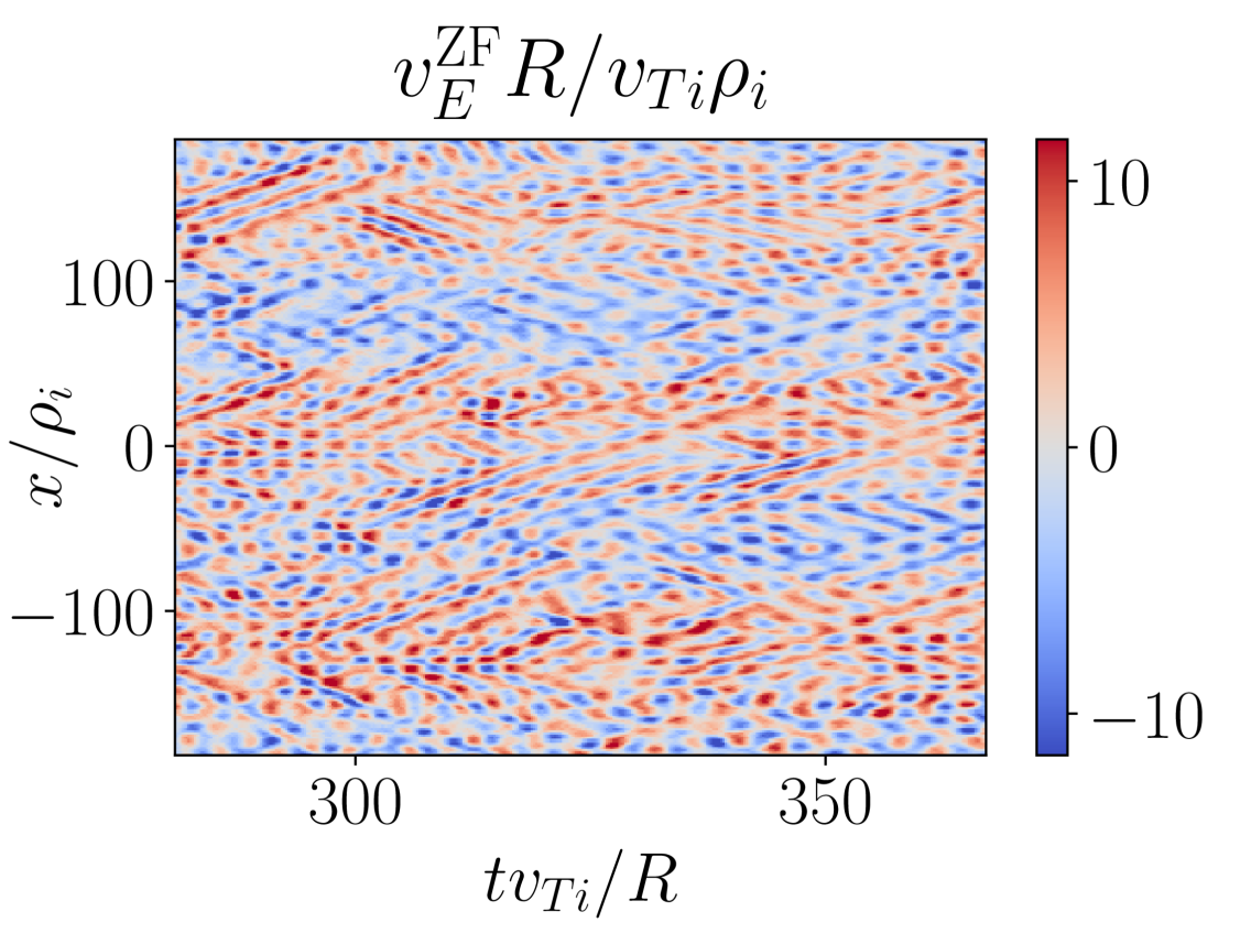
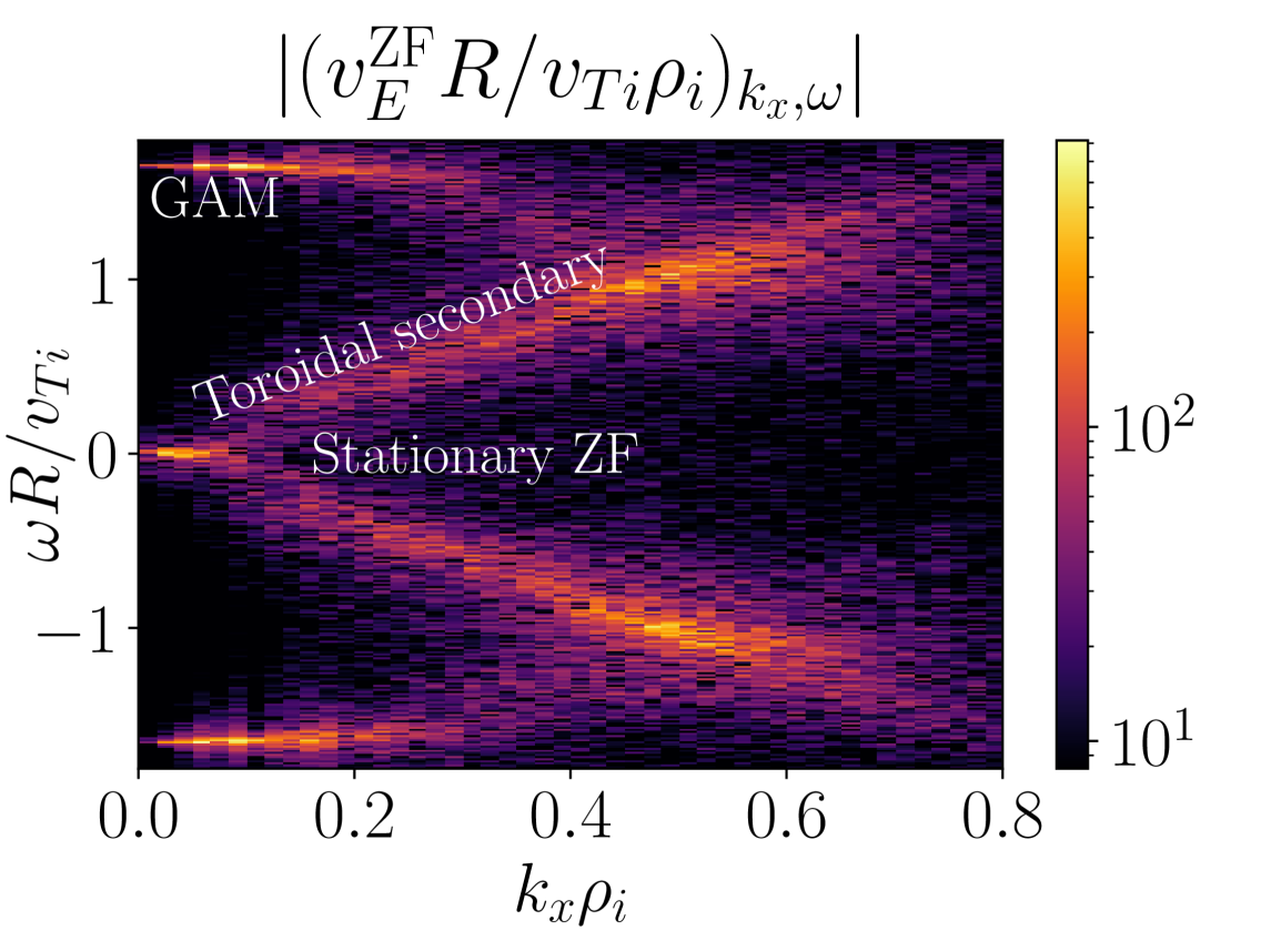
Figure 1: Zonal flow velocity $v_{E}^{\mathrm{ZF}}$ (see Section 2 for definition; other quantities in the figure follow the standard conventions and are also defined in Section 2) in real space (left) and Fourier space (right) from a nonlinear gyrokinetic simulation of tokamak ion-temperature-gradient turbulence with safety factor $q=4.2$. There are stationary ZFs and geodesic acoustic modes (GAMs) at large scales, and propagating ZFs at smaller radial scales corresponding to toroidal secondary modes. General information about the simulations shown in this study may be found in Section 2.3. Note that a similar plot for a different set of parameters was previously presented in Nies et al. (2024).

In this work, we develop a generalised theory of secondary modes including toroidal geometric effects neglected in previous studies, in particular the radial magnetic drift induced by toroidicity and the ensuing SW force. The theory describes a new branch of zonal flows, the toroidal secondary mode (TSM), which grows and propagates radially due to the SW force. Here, the up-down pressure asymmetry is generated through a combination of zonal flow shearing and the advection by the radial magnetic drift. The TSM is crucial to understand the ZF behaviour in simulations of tokamak ITG turbulence, see e.g. Figure 1, where the TSM explains the ZFs at short radial wavelengths – while the stationary ZFs and GAMs are found at long radial wavelengths. Moreover, the TSM was shown in previous work (Nies et al., 2024) to contribute to the saturation of strongly driven ITG turbulence in tokamaks.

The generalised theory of the secondary mode presented in this work also includes the ZF drive by nonlinear stresses. Therefore, the RDK secondary mode is recovered in the theory in the limit of strong nonlinear drive by the primary, in which case the linear coupling through the SW force becomes subdominant. Furthermore, the inclusion of the radial magnetic drift in the theory allows for the existence of ITG secondary modes (ISMs) driven unstable by the temperature gradient in the primary drive. The properties of the RDK secondary mode and the ISM will be discussed, as well as the connections between these modes and the TSM.

The paper is structured as follows: in Section 2, we first review the theory of gyrokinetics and the secondary mode model (Sections  2.1 and  2.2, respectively). We provide details of the numerical simulations (both of the turbulence and of the secondary mode) in Section 2.3. The theory of secondary modes in toroidal geometry is presented in Section 3, starting in Section 3.1 with the derivation of dispersion relations for the local (on a flux surface) ISMs and for the global (on a flux surface) TSM and RDK secondary mode. The ISM and the TSM are discussed in more detail in Sections 3.2 and 3.3, respectively. The strongly-driven non-resonant limit of the secondary modes is studied in Section 3.4. We evaluate the importance of various physical effects not considered in the theory of the generalised secondary mode in Section 3.5: the effects of binormal drifts and magnetic shear on the TSM are studied in Section 3.5.1 and the inclusion of parallel streaming is considered in Section 3.5.2. We summarise and discuss our results in Section 4. The limit of the secondary modes for strong primary drive and long perpendicular wavelengths is presented in A, and the RDK secondary mode dispersion relation for arbitrary radial wavelengths is derived in B.

2 Gyrokinetic secondary mode theory

We begin by reviewing in Section 2.1 the theory of gyrokinetics used to describe microinstabilities in strongly magnetised plasmas. The gyrokinetic secondary mode model will then be discussed in Section 2.2, and specifics of the gyrokinetic simulations performed in this work will be presented in Section 2.3.

2.1 Gyrokinetics

In the strongly magnetised plasmas typical of magnetic confinement fusion, the characteristic timescales of the microinstabilities that drive turbulence are much longer than the period of Larmor gyration. One may therefore average over the fast particle gyromotion and describe the evolution of rings of charge instead of that of particles. In the plasma core, one may further assume small-scale fluctuations compared to the Maxwellian background $F_{M\sigma}$, i.e. the distribution function $f_{\sigma}$ for any species $\sigma$ satisfies $\absolutevalue{\delta f_{\sigma}}=\absolutevalue{f_{\sigma}-F_{M\sigma}}\ll F_{M\sigma}$. For the collisionless and electrostatic limits considered in this study, the distribution of gyrocentres $g_{\sigma}=\langle\delta f_{\sigma}\rangle_{\mathop{}\!\boldsymbol{R}_{\sigma}}$ may then be shown to evolve according to the gyrokinetic (GK) equation (Catto, 1978; Frieman and Chen, 1982)

$$\partial_{t}g_{\sigma}+\left(v_{\parallel}\boldsymbol{\hat{b}}+\mathop{}\!\boldsymbol{\tilde{v}}_{M\sigma}\right)\cdot\nabla\left(g_{\sigma}+\frac{Z_{\sigma}e\langle\varphi\rangle_{\mathop{}\!\boldsymbol{R}_{\sigma}}}{T_{\sigma}}F_{M\sigma}\right)+\langle\mathop{}\!\boldsymbol{v}_{E}\rangle_{\mathop{}\!\boldsymbol{R}_{\sigma}}\cdot\nabla(F_{M\sigma}+g_{\sigma})=0,$$ (1)

where the derivatives are taken at constant particle energy $E_{\sigma}=m_{\sigma}(v_{\parallel}^{2}+v_{\perp}^{2})/2$ and magnetic moment $\mu_{\sigma}=m_{\sigma}v_{\perp}^{2}/2B$, with the parallel and perpendicular velocities being $v_{\parallel}=\mathop{}\!\boldsymbol{v}\cdot\boldsymbol{\hat{b}}$ and $v_{\perp}=|{\mathop{}\!\boldsymbol{v}\times\boldsymbol{\hat{b}}}|$, respectively. The gradients are performed with respect to the gyrocentre position $\mathop{}\!\boldsymbol{R}_{\sigma}=\mathop{}\!\boldsymbol{r}-\boldsymbol{\hat{b}}\times\mathop{}\!\boldsymbol{v_{\perp}}/\Omega_{\sigma}$, shifted from the real space position $\mathop{}\!\boldsymbol{r}$ by the gyroradius vector $\boldsymbol{\hat{b}}\times\mathop{}\!\boldsymbol{v}_{\perp}/\Omega_{\sigma}$. Here, $\boldsymbol{\hat{b}}=\mathop{}\!\boldsymbol{B}/B$ is the unit magnetic field vector, $B=|\mathop{}\!\boldsymbol{B}|$ is the magnetic field strength, and $Z_{\sigma}e$, $m_{\sigma}$, $v_{T\sigma}$, $T_{\sigma}=m_{\sigma}v_{T\sigma}^{2}/2$, and $\Omega_{\sigma}=Z_{\sigma}eB/m_{\sigma}$ are the particle charge, mass, thermal speed, temperature, and Larmor gyration frequency, respectively. Angular brackets $\langle\cdot\rangle_{\mathop{}\!\boldsymbol{r}}$ and $\langle\cdot\rangle_{\mathop{}\!\boldsymbol{R}_{\sigma}}$ denote gyro-averages at fixed real space position $\mathop{}\!\boldsymbol{r}$ and gyrocentre position $\mathop{}\!\boldsymbol{R}_{\sigma}$, respectively. Furthermore, $\mathop{}\!\boldsymbol{v}_{E}=\boldsymbol{\hat{b}}\times\nabla\varphi/B$ is the $\mathop{}\!\boldsymbol{E}\times\mathop{}\!\boldsymbol{B}$-velocity and $\mathop{}\!\boldsymbol{\tilde{v}}_{M\sigma}$ is the magnetic drift velocity. The tilde on $\mathop{}\!\boldsymbol{\tilde{v}}_{M\sigma}$ is meant to make it distinct from the quantity $v_{Mx}$ that we will introduce later in equation (10). The magnetic drift contains both the curvature and $\nabla B$-drifts and may be expressed as

$$\mathop{}\!\boldsymbol{\tilde{v}}_{M\sigma}=\rho_{\sigma}v_{T\sigma}\left(\frac{v_{\parallel}^{2}+v_{\perp}^{2}/2}{v_{T\sigma}^{2}}\frac{\mathop{}\!\boldsymbol{B}\times\nabla B}{B^{2}}+\frac{v_{\parallel}^{2}}{v_{T\sigma}^{2}}\mu_{0}\frac{\mathop{}\!\boldsymbol{B}\times\nabla p}{B^{3}}\right),$$ (2)

where $\rho_{\sigma}=v_{T\sigma}/\Omega_{\sigma}$ is the gyroradius of a thermal particle and $\mu_{0}$ is the vacuum permeability. The curvature drift contribution was simplified in (2) by assuming ideal magnetohydrostatic force balance $(\nabla\times\mathop{}\!\boldsymbol{B})\times\mathop{}\!\boldsymbol{B}=\mu_{0}\nabla p$, with $\nabla p$ the background pressure gradient. The electrostatic potential fluctuation $\varphi$ in the GK equation (1) must be determined self-consistently from quasineutrality

$$0=\sum_{\sigma}Z_{\sigma}\int\mathrm{d}^{3}v\,\delta f_{\sigma}=\sum_{\sigma}Z_{\sigma}\int\mathrm{d}^{3}v\;\langle g_{\sigma}\rangle_{\mathop{}\!\boldsymbol{r}}-\sum_{\sigma}\frac{Z_{\sigma}^{2}en_{\sigma}}{T_{\sigma}}\left(1-\hat{\Gamma}_{0\sigma}\right)\varphi,$$ (3)

where

$$\hat{\Gamma}_{0\sigma}\varphi\equiv\frac{1}{n_{\sigma}}\int\mathrm{d}^{3}v\,F_{M\sigma}\langle\langle\varphi\rangle_{\mathop{}\!\boldsymbol{R}_{\sigma}}\rangle_{\mathop{}\!\boldsymbol{r}}.$$ (4)

The charge density in the quasineutrality equation (3) has contributions from the density of gyrocentres $\int\mathrm{d}^{3}v\;\langle g_{\sigma}\rangle_{\mathop{}\!\boldsymbol{r}}$ and from the polarisation of gyro-orbits, which is proportional to $\left(1-\hat{\Gamma}_{0\sigma}\right)\varphi$.

In this study, we will consider ion-scale fluctuations, with typical spatial variation perpendicular to the magnetic field on the ion gyroradius scale, $\nabla_{\perp}\ln g_{\sigma}\sim\rho_{i}^{-1}$, and typical temporal variation on an ion transit time, $\partial_{t}\ln g_{\sigma}\sim v_{Ti}/R$. Here, $R$ is the major radius of the tokamak or stellarator under consideration and is taken to be the system scale length. While the typical scale length of the turbulence in the directions perpendicular to the magnetic field is on the ion gyroradius scale $\rho_{i}$, its parallel extent is on the much larger system scale $R$, with $R\gg\rho_{i}$ in a strongly magnetised plasma. Therefore, the turbulence may be modelled in a perpendicularly narrow flux tube centered on a chosen flux surface with enclosed toroidal flux $\psi=\psi_{0}$ and on a chosen field line $\alpha=\alpha_{0}$. The field line label $\alpha$ is defined such that $\mathop{}\!\boldsymbol{B}=\nabla\psi\times\nabla\alpha$. A set of coordinates $(x,y,\theta)$ is used to parametrise the flux tube, with $x$ labelling flux surfaces, $y$ labelling field lines within a flux surface, and the distance along the magnetic field chosen here to be parametrised by the poloidal angle $\theta$ without loss of generality. The coordinates $x$ and $y$ vary on the ion gyroradius scale. Therefore, all background (non-fluctuating) quantities are evaluated at $(\psi_{0},\alpha_{0}$) and are independent of $x$ and $y$ to leading order in $\rho_{i}/R\ll 1$. As a consequence, statistical periodicity may be assumed to hold in $x$ and $y$ for the fluctuating quantities, so that the fluctuating gyrocentre distribution and electrostatic potential may be expanded in Fourier harmonics

$$g_{\sigma}=\sum_{k_{x},k_{y}}\hat{g}_{\sigma}(k_{x},k_{y},\theta,v_{\parallel},v_{\perp})e^{i(k_{x}X_{\sigma}+k_{y}Y_{\sigma})},\qquad\varphi=\sum_{k_{x},k_{y}}\hat{\varphi}(k_{x},k_{y},\theta)e^{i(k_{x}x+k_{y}y)}.$$ (5)

Due to their comparatively fast propagation speed, the electrons may be modelled by a modified adiabatic response

$$\delta f_{e}=\frac{e}{T_{e}}\left(\varphi-\langle\varphi\rangle_{\psi}\right)F_{Me}.$$ (6)

The substraction of the flux-surface averaged potential $\langle\varphi\rangle_{\psi}$ stems from the electrons’ fast motion along magnetic field lines ($v_{Te}\sim v_{Ti}\sqrt{m_{i}/m_{e}}\gg v_{Ti}$) and small gyroradii ($\rho_{e}\sim\rho_{i}\sqrt{m_{e}/m_{i}}\ll\rho_{i}$). Due to these differences with ions, electrons can only respond to in-surface variations of the electrostatic potential. Here, the flux-surface average is defined as

$$\langle f\rangle_{\psi}=\int\frac{\mathrm{d}\theta}{\mathop{}\!\boldsymbol{B}\cdot\nabla\theta}\,f^{\mathrm{Z}}\bigg{/}\int\frac{\mathrm{d}\theta}{\mathop{}\!\boldsymbol{B}\cdot\nabla\theta}\equiv\langle\langle f\rangle_{y}\rangle_{\theta},$$ (7)

where the zonal and nonzonal components of any quantity $f$ are defined as $f^{\mathrm{Z}}=\langle f\rangle_{y}=\sum_{k_{x}}\hat{f}(k_{x},k_{y}=0,\theta)e^{ik_{x}x}$ and $f^{\mathrm{NZ}}=f-f^{\mathrm{Z}}$, respectively. The $\theta$-integral in (7) extends over the length of the flux tube, $\theta\in[-\pi N_{\mathrm{turns}},\pi N_{\mathrm{turns}}]$, where $N_{\mathrm{turns}}$ is generally chosen to be an integer for tokamak simulations but may be a non-integer real for stellarator simulations.

Using the modified adiabatic electron response (6) and assuming a single ion species $i$ for simplicity, the quasineutrality equation (3) simplifies to

$$\left(1-\hat{\Gamma}_{0i}\right)\varphi+\tau\left(\varphi-\langle\varphi\rangle_{\psi}\right)=\frac{T_{i}}{Z_{i}en_{i}}\int\mathrm{d}^{3}v\,\langle g_{i}\rangle_{\mathop{}\!\boldsymbol{r}},$$ (8)

where $n_{i}$ is the background ion density and $\tau=T_{i}/Z_{i}T_{e}$ gives the ratio of ion and electron temperatures.

The modified adiabatic electron response crucially reduces the ZF inertia at long perpendicular wavelengths, where $\hat{\Gamma}_{0i}\approx 1$. This may be seen explicitly by taking the time derivative and flux-surface average of (8) and inserting (1), which leads to the vorticity equation

$$\left\langle\left(1-\hat{\Gamma}_{0i}\right)\partial_{t}\varphi\right\rangle_{\psi}=-\frac{T_{i}}{Z_{i}en_{i}}\left\langle\mathrm{d}^{3}v\,\left\langle\langle\mathop{}\!\boldsymbol{v}_{E}\rangle_{\mathop{}\!\boldsymbol{R}_{i}}\cdot\nabla g_{i}+\tilde{v}_{Mx}\partial_{x}\left(g_{i}+\frac{Z_{i}e\langle\varphi\rangle_{\mathop{}\!\boldsymbol{R}_{i}}}{T_{i}}F_{Mi}\right)\right\rangle_{\mathop{}\!\boldsymbol{r}}\right\rangle_{\psi}.$$ (9)

The vorticity equation describes the time evolution of the ZF velocity due to nonlinear stresses and due to the Stringer-Winsor force induced by the ion radial magnetic drift velocity

$$\tilde{v}_{Mx}\equiv\tilde{\mathop{}\!\boldsymbol{v}}_{Mi}\cdot\nabla x=\rho_{i}v_{Ti}\frac{\mathop{}\!\boldsymbol{B}\times\nabla B\cdot\nabla x}{B^{2}}\frac{v_{\parallel}^{2}+v_{\perp}^{2}/2}{v_{Ti}^{2}}\equiv v_{Mx}\frac{v_{\parallel}^{2}+v_{\perp}^{2}/2}{v_{Ti}^{2}},$$ (10)

where we used the fact that the background pressure $p=p(\psi)$ in (2) is a flux function. Note that (10) implicitly defines the velocity-independent quantity $v_{Mx}$ that will turn out to be convenient below.

Since the $\theta$-variation of the zonal potential $\varphi^{\mathrm{Z}}$ is generally small due to the electron response in the quasineutrality equation (8), we refer to $v_{E}^{\mathrm{ZF}}=\langle\mathop{}\!\boldsymbol{v}_{E}\cdot\nabla y\rangle_{\psi}$ as the zonal flow (ZF).

2.2 Secondary model

In this study, the growth of ZFs is modelled by describing the dynamics of small-amplitude secondary modes over a primary background frozen in time. The ion gyrocentre distribution is expanded as $g_{i}=g_{i}^{P}+g_{i}^{S}$ with $\absolutevalue{g_{i}^{S}}\ll\absolutevalue{g_{i}^{P}}$, allowing the GK equation (1) to be linearised to

$$\partial_{t}g_{i}^{S}+\left(v_{\parallel}\boldsymbol{\hat{b}}+\mathop{}\!\boldsymbol{\tilde{v}}_{Mi}\right)\cdot\nabla\left(g_{i}^{S}+\frac{Z_{i}e\langle\varphi^{S}\rangle_{\mathop{}\!\boldsymbol{R}_{i}}}{T_{i}}F_{Mi}\right)+\langle\mathop{}\!\boldsymbol{v}_{E}^{S}\rangle_{\mathop{}\!\boldsymbol{R}_{i}}\cdot\nabla(F_{Mi}+g_{i}^{P})+\langle\mathop{}\!\boldsymbol{v}_{E}^{P}\rangle_{\mathop{}\!\boldsymbol{R}_{i}}\cdot\nabla g_{i}^{S}=0.$$ (11)

The secondary potential $\varphi^{S}$ is self-consistently determined by quasineutrality (8)

$$\left(1-\hat{\Gamma}_{0i}\right)\varphi^{S}+\tau\left(\varphi^{S}-\langle\varphi^{S}\rangle_{\psi}\right)=\frac{T_{i}}{Z_{i}en_{i}}\int\mathrm{d}^{3}v\,\langle g_{i}^{S}\rangle_{\mathop{}\!\boldsymbol{r}}.$$ (12)

The primary drive is assumed to be purely nonzonal, i.e. $\langle g_{i}^{P}\rangle_{y}=0$, as is the case for linearly unstable modes in gyrokinetics. In contrast, the secondary distribution $g_{i}^{S}$ has both zonal and nonzonal components. The purely growing RDK secondary mode was derived in Rogers et al. (2000) by further considering the limit of negligible linear terms $v_{\parallel}\boldsymbol{\hat{b}}\cdot\nabla,\mathop{}\!\boldsymbol{\tilde{v}}_{Mi}\cdot\nabla$, and $\langle\mathop{}\!\boldsymbol{v}_{E}^{S}\rangle_{\mathop{}\!\boldsymbol{R}_{i}}\cdot\nabla F_{Mi}$ in (11). Furthermore, the primary drive was assumed in Rogers et al. (2000) to be a streamer, i.e. $\partial_{x}g_{i}^{P}=0$, as they investigated fast growing secondary modes ‘catching up’ to a linearly unstable primary mode, and the streamers are generally the most unstable modes. The streamer primary drive assumption $\partial_{x}g_{i}^{P}=0$ can be relaxed, as shown in A where the secondary mode theory is rederived allowing for radial variation of the primary drive, in the strongly driven and long perpendicular wavelength limit.

In the main text of this paper, we will consider a frozen streamer primary drive ($\partial_{x}g_{i}^{P}=0,\partial_{t}g_{i}^{P}=0$) for simplicity. Aside from the scenario of a secondary mode catching up to a primary mode, this assumption may also be motivated by a separation of scales between the small-scale fast-oscillating secondary modes and a primary turbulent background slowly varying in $x$ and $t$. This scale separation is indeed satisfied in strongly-driven ITG turbulence (Nies et al., 2024), whence the secondary model is apt to describe the ZF behaviour in nonlinear turbulence simulations.

Motivated by the small radial scale of the toroidal secondary modes shown in Figure 1, we will further consider in the theory large binormal scales compared to the small radial wavelength $\absolutevalue{\partial_{y}\ln g_{i}^{S}}\ll\absolutevalue{\partial_{x}\ln g_{i}^{S}}$ (the case of comparable binormal and radial scales is studied numerically in Section 3.5.1). We thus neglect in (11) the magnetic drift advection in the binormal direction and the diamagnetic drift contribution $\langle\mathop{}\!\boldsymbol{v}_{E}^{S}\rangle_{\mathop{}\!\boldsymbol{R}_{i}}\cdot\nabla F_{Mi}\propto\partial_{y}\langle\varphi^{S}\rangle_{\mathop{}\!\boldsymbol{R}_{i}}$. Note the field-line labelling coordinate is $y\propto\alpha=\zeta-q\theta+\nu(\theta,\zeta)$, with a single-valued function $\nu$, the safety factor $q=q(x)$ measuring the average pitch of magnetic field lines on a flux surface, and a set of arbitrary poloidal and toroidal angles $\theta$ and $\zeta$, respectively. Therefore, its gradient

$$\nabla y\propto(1+\partial_{\zeta}\nu)\nabla\zeta+(-q+\partial_{\theta}\nu)\nabla\theta-\theta\,\nabla x\frac{\mathrm{d}q}{\mathrm{d}x}$$ (13)

has a secularly increasing component along the field line due to magnetic shear $\hat{s}\equiv\mathrm{d}\ln q/\mathrm{d}\ln x$. The assumed limit of negligible $\mathop{}\!\boldsymbol{\tilde{v}}_{Mi}\cdot\nabla y$ thus also requires $\absolutevalue{\partial_{y}\ln g_{i}^{S}\hat{s}\theta}\ll\absolutevalue{\partial_{x}\ln g_{i}^{S}}$, i.e. we exclude modes that are very extended along the magnetic field in our analysis. The Fourier modes in $k_{x}$ of the secondary mode then become eigenmodes of the system. Had we kept the magnetic shear in our derivation, the Fourier modes in $k_{x}$ would otherwise be coupled.

With our assumptions, the gyro-averages simplify to Bessel functions

$$J_{0i}=J_{0}\left(\sqrt{2b_{i}}\,\frac{v_{\perp}}{v_{Ti}}\right),$$ (14)

with the factor $b_{i}$ (not to be confused with the unit magnetic field vector $\boldsymbol{\hat{b}}$) measuring the strength of the finite Larmor Radius (FLR) effects,

$$b_{i}=\frac{k_{x}^{2}\absolutevalue{\nabla x}^{2}\rho_{i}^{2}}{2}.$$ (15)

If we further consider exponentially growing solutions, an equation for the secondary eigenmodes $g_{i}^{S}=\hat{g}_{i}^{S}e^{i(k_{x}X_{i}-\omega t)},\varphi^{S}=\hat{\varphi}^{S}e^{i(k_{x}x-\omega t)}$ is readily derived from (11),

$$0=-\omega\hat{g}_{i}^{S}+\left(-iv_{\parallel}\boldsymbol{\hat{b}}\cdot\nabla+k_{x}\tilde{v}_{Mx}\right)\left(\hat{g}_{i}^{S}+\frac{Z_{i}e\hat{\varphi}^{S}}{T_{i}}J_{0i}F_{Mi}\right)-k_{x}\tilde{v}_{g}^{P}\frac{Z_{i}e\hat{\varphi}^{S}}{T_{i}}J_{0i}F_{Mi}+k_{x}v_{Ex}^{P}\hat{g}_{i}^{S}.$$ (16)

Here, we defined the radial $\mathop{}\!\boldsymbol{E}\times\mathop{}\!\boldsymbol{B}$-velocity associated with the primary,

$$v_{Ex}^{P}=\mathop{}\!\boldsymbol{v}_{E}^{P}\cdot\nabla x=-\frac{\boldsymbol{\hat{b}}\times\nabla x\cdot\nabla y}{B}\partial_{y}\varphi^{P}$$ (17)

and the function (with velocity units)

$$\tilde{v}_{g}^{P}=-\frac{T_{i}}{Z_{i}e}\frac{\boldsymbol{\hat{b}}\times\nabla x\cdot\nabla y}{B}\frac{\partial_{y}g_{i}^{P}}{F_{Mi}}.$$ (18)

Owing to the gyro-averages becoming Bessel functions, the integral (4) simplifies to $\hat{\Gamma}_{0i}=\Gamma_{0i}\equiv I_{0}(b_{i})e^{-b_{i}}$ with $I_{0}$ the modified Bessel function of the first kind. The quasineutrality equation (12) in Fourier space then becomes

$$\left(1-\Gamma_{0i}\right)\hat{\varphi}^{S}+\tau\left(\hat{\varphi}^{S}-\langle\hat{\varphi}^{S}\rangle_{\psi}\right)=\frac{T_{i}}{Z_{i}en_{i}}\int\mathrm{d}^{3}v\,J_{0i}\hat{g}_{i}^{S}.$$ (19)

2.3 Gyrokinetic simulations

All simulations presented in this study use the code stella (Barnes et al., 2019) to model a hydrogenic plasma ($Z_{i}=1$) on the flux surface at half-radius $r(\psi_{0})=a/2$ of the Cyclone Base Case, a tokamak with flux surfaces of circular cross-section and minor radius $a=0.36R$. The radial coordinate is $x=r-r(\psi_{0})$ and the binormal coordinate is $y=\alpha r(\psi_{0})/q(\psi_{0})$. The electrons follow the modified adiabatic response (6) and the ratio of ion to electron temperatures is set to $\tau=1$. The flux tube is chosen to extend over a single poloidal turn, $N_{\mathrm{turns}}=1$. The safety factor $q$ is frequently varied across simulations and is thus specified in the captions of the respective figures. In all simulations but those of Figure 9, the magnetic shear $\hat{s}\equiv\mathrm{d}\ln q/\mathrm{d}\ln x$ measuring the radial variation of the field line pitch is set to $\hat{s}=0.8$.

Two types of GK simulations are presented in this study. First, the zonal flows from fully nonlinear GK simulations of ITG turbulence are studied in Figures 1 and 10. In these cases, a background temperature gradient $R/L_{Ti}=-R\,\mathrm{d}\ln T_{i}/\mathrm{d}r=13.9$ and background density gradient $R/L_{n}=-R\,\mathrm{d}\ln n_{i}/\mathrm{d}r=2.2$ are assumed. The twist-and-shift boundary condition (Beer et al., 1995) is used at the ends of the flux-tube domain,

$$\hat{g}_{\sigma}(k_{x},k_{y},\theta=\pi N_{\mathrm{turns}})=\hat{g}_{\sigma}(k_{x}+2\pi N_{\mathrm{turns}}\hat{s}k_{y},k_{y},\theta=-\pi N_{\mathrm{turns}}),$$ (20)

such that different radial wavenumbers are coupled through the magnetic shear. The box size in the binormal and radial directions is $L_{y}=2\pi/\min(k_{y})=377\rho_{i}$ and $L_{x}=2\pi/\min(k_{x})=375\rho_{i}$, respectively. The simulations include perpendicular wavenumbers up to $k_{y}\rho_{i}=1.42$ and $k_{x}\rho_{i}=2.13$, with a parallel resolution of $N_{\theta}=32$. The velocity-space resolutions are $N_{v_{\parallel}}=32$ for the parallel velocity grid and $N_{\mu}=8$ for the magnetic moment grid. Parallel velocities between $-3v_{Ti}$ and $3v_{Ti}$ are considered, and the maximum of $\mu$ is chosen such that the maximum perpendicular velocity is $3v_{Ti}$ at the minimum value of $B$.

In all other GK simulations (Figures 2(a), 3, 4, 5, 6, 7(b), 8, 9, and 11), the secondary system of equations (11) and (12) is solved to obtain the complex frequency of exponentially growing secondary modes at a specified radial wavenumber $k_{x}\neq 0$. In these simulations, the $(k_{x}=0,k_{y}=k_{y}^{P}$) Fourier mode is enforced to be constant in time to represent the streamer primary mode, i.e. a slowly growing linear mode or a slowly evolving turbulent background. For simplicity, the primary drive is thus always chosen in simulations to vary sinusoidally in the binormal coordinate $y$ (in contrast, the theory of Section 3 allows for arbitrary $y$-variation). Unless stated otherwise, the GK simulations of the secondary are performed with binormal resolution $N_{y}=32$, parallel resolution $N_{\theta}=96$, parallel velocity resolution $N_{v_{\parallel}}=72$, and magnetic moment resolution $N_{\mu}=16$.

In this study, the strength of the primary drive is characterised through the normalised amplitude

$$\mathcal{A}^{P}\equiv\sqrt{\left\langle\left(\frac{v_{Ex}^{P}}{v_{Ti}}\frac{R}{\rho_{i}}\right)^{2}\right\rangle_{\psi}},$$ (21)

which gives a measure of the relative strengths of the primary $\mathop{}\!\boldsymbol{E}\times\mathop{}\!\boldsymbol{B}$ flow velocity and the radial magnetic drift velocity $v_{Mx}\sim\rho_{i}v_{Ti}/R$. In Nies et al. (2024), GK simulations of the secondary mode were shown for an ITG eigenmode taken as the primary drive. To allow for a direct comparison between GK simulations and the secondary mode theory that we will present below, the primary drive is here set to be a bi-Maxwellian with density $n^{P}$, parallel temperature $T_{\parallel}^{P}$, and perpendicular temperature $T_{\perp}^{P}$, i.e.

$$g_{i}^{P}=F_{Mi}\left[\frac{n^{P}}{n_{i}}+\frac{T_{\parallel}^{P}}{T_{i}}\left(\frac{v_{\parallel}^{2}}{v_{Ti}^{2}}-\frac{1}{2}\right)+\frac{T_{\perp}^{P}}{T_{i}}\left(\frac{v_{\perp}^{2}}{v_{Ti}^{2}}-1\right)\right].$$ (22)

We choose to consider parallel and perpendicular primary temperatures separately as they contribute differently to the growth of various secondary modes. In particular, the RDK secondary modes will be shown to depend only on $T_{\perp}^{P}$ as they rely on finite Larmor radius effects and the gyroradius size depends only on the perpendicular particle energy, see also (14). In contrast, the TSM instability mechanism hinges on the radial magnetic drift (10), which depends on both parallel and perpendicular particle energy.

For the model primary drive (22), equation (18) simplifies to

$$\tilde{v}_{g}^{P}=\tau v_{Ex}^{P}\left[1+\eta_{\parallel}^{P}\left(\frac{v_{\parallel}^{2}}{v_{Ti}^{2}}-\frac{1}{2}\right)+\eta_{\perp}^{P}\left(\frac{v_{\perp}^{2}}{v_{Ti}^{2}}-1\right)\right].$$ (23)

Here, we defined the dimensionless ratios of the primary parallel and perpendicular temperature gradients to its density gradient,

$$\eta_{\parallel}^{P}=\frac{n_{i}}{T_{i}}\frac{\partial_{y}T_{\parallel}^{P}}{\partial_{y}n^{P}},\qquad\eta_{\perp}^{P}=\frac{n_{i}}{T_{i}}\frac{\partial_{y}T_{\perp}^{P}}{\partial_{y}n^{P}},$$ (24)

and used quasineutrality (8) in the limit of long binormal wavelengths to relate the primary density and potential. Arbitrary variations in $y$ and $\theta$ of $v_{Ex}^{P}$, $\eta_{\parallel}^{P}$, and $\eta_{\perp}^{P}$ are allowed in the theory. However, in the simulations, $\eta_{\parallel}^{P}$ and $\eta_{\perp}^{P}$ are taken to be constants and the primary drive’s variation on the flux surface is captured entirely by $v_{Ex}^{P}(y,\theta)$, with the exception of the simulations in Figure 3(b) where a phase shift in $y$ between the density and temperature moments of the primary distribution function is considered. The variation of the primary drive $v_{Ex}^{P}(y,\theta)$ along the magnetic field for each simulation is specified in the corresponding figures.

The primary mode’s binormal wavenumber $k_{y}^{P}\rho_{i}=10^{-3}$ is chosen to be small in all simulations (except those of Figure 9) to ensure our neglect of binormal derivatives and magnetic shear is justified. In this limit, the dynamics at different radial wavenumbers are effectively decoupled, and we therefore impose the phase-shift-periodic boundary condition (St-Onge et al., 2022; Volčokas et al., 2023)

$$\hat{g}_{\sigma}(k_{x},k_{y},\theta=\pi N_{\mathrm{turns}})=\exp\left(ik_{y}L_{y}\Theta\right)\hat{g}_{\sigma}(k_{x},k_{y},\theta=-\pi N_{\mathrm{turns}})$$ (25)

in the GK simulations of the secondary mode, with $L_{y}=2\pi/\min(k_{y})$ the size of the binormal domain. We note that the zonal modes ($k_{y}=0$) always satisfy periodic boundary conditions, as may be seen in (20) and (25). The phase-shift-periodic boundary condition (25) models a flux surface with zero magnetic shear. The flux surface is rational if $\Theta\in\mathbb{Z}$ and irrational if $\Theta\in\mathbb{R}\setminus\mathbb{Z}$. In practice, this boundary condition is chosen because it does not couple different $k_{x}$ Fourier modes. The choice of $\Theta$ will dictate the degree of decorrelation at the ends of the flux tube; e.g., small $\Theta$ values allow modes to remain coherent after wrapping around the flux tube. We will show that most results of interest are not affected by this boundary condition because the choice of boundary conditions is important for the secondary modes only when the parallel streaming contribution to (16) is relevant to the dynamics; some discussion of these effects will be provided in Section 3.5.2.

3 Secondary modes in toroidal geometry

An overview of the secondary modes discussed in this study is shown in Figure 2 for varying radial wavenumber $k_{x}$ and primary amplitude $\mathcal{A}^{P}$. In addition to the purely growing RDK secondary mode at large $\mathcal{A}^{P}$, growing TSMs and ISMs with finite $\omega_{r}$ are observed at smaller $\mathcal{A}^{P}$.

After deriving the theory of the various secondary modes in Section 3.1, the ISM and TSM will be discussed in Sections 3.2 and 3.3, respectively. Then, the non-resonant limit of the secondary modes will be considered in Section 3.4, including the RDK limit (see also A). Finally, the effects of finite binormal wavenumbers and parallel streaming will be studied in Section 3.5, including a discussion of the Landau damping threshold for the TSM (see Figure 2(b)) in Section 3.5.2.

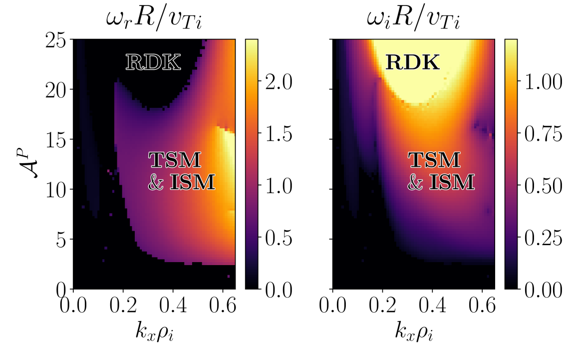
(a) Secondary mode real frequency (left) and growth rate (right) from gyrokinetic simulations. The primary distribution is given by (22) with $\eta_{\parallel}^{P}=\eta_{\perp}^{P}=2$ and varies along the magnetic field as $g_{i}^{P}\propto e^{-(\theta/\pi)^{2}}$. The safety factor is set to $q=2.8$. The parallel boundary condition is the phase-shift-periodic boundary condition (25) with $\Theta=0.288572618$. Due to computational cost, the simulations are performed with a reduced resolution $\{N_{y},N_{\theta},N_{v_{\parallel}},N_{\mu}\}=\{16,48,32,8\}$.

(b) Approximate regions of Rogers-Dorland-Kotschenreuther (RDK) secondary mode (Rogers et al., 2000), toroidal secondary mode (TSM) (Nies et al., 2024), and ITG secondary mode (ISM). The parallel streaming frequency is $\omega_{\parallel}\sim v_{\parallel}\hat{b}\cdot\nabla\sim v_{Ti}/qR$ and the geodesic acoustic mode (GAM) frequency is $\omega_{\mathrm{GAM}}\sim v_{Mx}/\rho_{i}\sim v_{Ti}/R$ (50).

Figure 2: Illustrative case of secondary modes in the space of the primary amplitude $\mathcal{A}^{P}$ and secondary radial wavenumber $k_{x}$ (a), and qualitative picture (b). The TSM ($\omega_{r}\neq 0$) is found at short radial wavelengths $k_{x}\gtrsim\omega_{\parallel}/v_{Mx}$ as it is Landau damped at long radial wavelengths (Section 3.5.2), and above a primary amplitude threshold $\mathcal{A}^{P}\gtrsim 1$ as it is otherwise subject to kinetic damping by the radial magnetic drift (Section 3.3). The RDK secondary mode ($\omega_{r}=0$) is found at large primary amplitudes, $k_{x}\tilde{v}_{g}^{P}\gtrsim\omega_{\mathrm{GAM}}$ for short wavelengths $k_{x}\gtrsim\omega_{\parallel}/v_{Mx}$ (Section 3.4), and $k_{x}\tilde{v}_{g}^{P}\gtrsim\omega_{\parallel}$ for long wavelengths $k_{x}\lesssim\omega_{\parallel}/v_{Mx}$ (Section 3.5.2). The horizontally dashed region in (b) is indicative of the non-resonant limit of the toroidal secondary mode (Section 3.4), between the TSM and RDK regions. The ISMs, discussed in Section 3.2, are dominant at short wavelengths $k_{x}\gtrsim\omega_{\parallel}/v_{Mx}$ for weak primary drive $\mathcal{A}^{P}\sim 1$, and at sub-Larmor scales $k_{x}\rho_{i}\gtrsim 1$. The diagonally hashed regions in (b) have weak primary drive $k_{x}\tilde{v}_{g}^{P}\lesssim\omega_{\parallel}$; the comparatively fast parallel streaming rate then makes the choice of parallel boundary condition important and the assumptions made in our secondary mode theory may become inappropriate (Section 3.5.2). Note that the size and shape of the regions can vary depending on the parameters used, e.g. the phase-space dependence of the primary drive or the magnetic geometry.

3.1 Theory of ITG and toroidal secondary modes

We consider the limit where the effects of parallel streaming are negligible, e.g. by considering a tokamak with a large safety factor, as $v_{\parallel}\boldsymbol{\hat{b}}\cdot\nabla\sim v_{Ti}/qR$. The required size of $q$ to make the parallel streaming sufficiently small depends on the primary amplitude and the radial wavenuber under consideration, as will be discussed further in Section 3.5.2. In the absence of parallel streaming, the GK equation for the secondary eigenmodes (16) simplifies to an algebraic equation

$$0=-\omega\hat{g}_{i}^{S}+k_{x}\tilde{v}_{Mx}\left(\hat{g}_{i}^{S}+\frac{Z_{i}e\hat{\varphi}^{S}}{T_{i}}J_{0i}F_{Mi}\right)-k_{x}\tilde{v}_{g}^{P}\frac{Z_{i}e\hat{\varphi}^{S}}{T_{i}}J_{0i}F_{Mi}+k_{x}v_{Ex}^{P}\hat{g}_{i}^{S},$$ (26)

with solution

$$\hat{g}_{i}^{S}=\frac{k_{x}\tilde{v}_{Mx}-k_{x}\tilde{v}_{g}^{P}}{\omega-k_{x}v_{Ex}^{P}-k_{x}\tilde{v}_{Mx}}J_{0i}F_{Mi}\frac{Z_{i}e\hat{\varphi}^{S}}{T_{i}}.$$ (27)

Inserting (27) into the quasineutrality equation (19) and rearranging, we obtain

$$\tau\langle\hat{\varphi}^{S}\rangle_{\psi}=\hat{\varphi}^{S}\left(1-\Gamma_{0i}+\tau-\mathcal{N}\right),$$ (28)

where we defined

$$\mathcal{N}=\frac{1}{n_{i}}\int\mathrm{d}^{3}v\,J_{0i}^{2}F_{Mi}\frac{k_{x}\tilde{v}_{Mx}-k_{x}\tilde{v}_{g}^{P}}{\omega-k_{x}v_{Ex}^{P}-k_{x}\tilde{v}_{Mx}}.$$ (29)

Equation (28) has two classes of solutions. First, when the zonal flow component of the secondary mode vanishes ($\langle\hat{\varphi}^{S}\rangle_{\psi}=0$), there are local modes on the flux surface (at a given $y$ and $\theta$) where

$$0=\mathcal{D}^{\mathrm{ISM}}(y,\theta)\equiv\left(1-\Gamma_{0i}+\tau-\mathcal{N}\right)/\tau.$$ (30)

These modes may be identified as local ISMs driven unstable by the gradients in the primary drive. They will be discussed further in Section 3.2.

The second class of solutions to (28) corresponds to secondary modes with nonzero zonal flow component $\langle\hat{\varphi}^{S}\rangle_{\psi}\neq 0$, which will be our principal focus. The corresponding dispersion relation is derived from (28) and the consistency condition $1=\langle\hat{\varphi}^{S}/\langle\hat{\varphi}^{S}\rangle_{\psi}\rangle_{\psi}$,

$$0=\mathcal{D}\equiv 1-\left\langle\frac{1}{\mathcal{D}^{\mathrm{ISM}}}\right\rangle_{\psi}=1-\left\langle\frac{\tau}{1-\Gamma_{0i}+\tau-\mathcal{N}}\right\rangle_{\psi}.$$ (31)

These modes are global on the flux surface: once the mode frequency has been obtained by solving (31), the shape of the eigenfunction in $y$ and $\theta$ is given by (28). As we will show explicitly below (see Section 3.4), the dispersion relation (31) includes the TSM, the RDK secondary mode, and the GAM.

To evaluate the dispersion relations numerically, we follow the procedure of Terry et al. (1982) and Biglari et al. (1989) and express the resonant denominator in (29) as

$$\frac{1}{\omega-k_{x}v_{Ex}^{P}-k_{x}\tilde{v}_{Mx}}=-i\int_{0}^{\infty}\mathrm{d}\lambda\,\exp\left[i\lambda(\omega-k_{x}v_{Ex}^{P}-k_{x}\tilde{v}_{Mx})\right],$$ (32)

where we assumed exponentially growing secondary modes ($\omega_{i}>0$) so that the $\lambda$-integral converges at infinity. If we further assume a bi-Maxwellian primary distribution function (22), the parallel and perpendicular velocity integrals in (29) may be evaluated to give

$$\mathcal{N} =-2i\int_{0}^{\infty}\mathrm{d}\lambda\,\frac{e^{i\lambda(\omega-k_{x}v_{Ex}^{P})}}{\left(1+i\lambda k_{x}v_{Mx}\right)^{1/2}\left(2+i\lambda k_{x}v_{Mx}\right)}\Bigg{[}\left(\Gamma_{0i}(\tilde{b}_{i})+\tilde{b}_{i}\Gamma_{0i}^{\prime}(\tilde{b}_{i})\right)\frac{k_{x}v_{Mx}-2\tau k_{x}v_{Ex}^{P}\eta_{\perp}^{P}}{2+i\lambda k_{x}v_{Mx}}$$

$$+\Gamma_{0i}(\tilde{b}_{i})\left(\tau k_{x}v_{Ex}^{P}\left(\frac{\eta_{\parallel}^{P}}{2}+\eta_{\perp}^{P}-1\right)+\frac{k_{x}v_{Mx}-\tau k_{x}v_{Ex}^{P}\eta_{\parallel}^{P}}{2(1+i\lambda k_{x}v_{Mx})}\right)\Bigg{]},$$ (33)

where $\Gamma_{0i}^{\prime}(\tilde{b}_{i})=\mathrm{d}\Gamma_{0i}(\tilde{b}_{i})/\mathrm{d}\tilde{b}_{i}$ and

$$\tilde{b}_{i}=\frac{2b_{i}}{2+i\lambda k_{x}v_{Mx}}.$$ (34)

The integrand in (3.1) decays exponentially at large $\lambda$ as $\omega_{i}>0$ and the integral may be evaluated efficiently numerically.

The dispersion relations (30) and (31) are validated against gyrokinetic simulations in Figure 3. Excellent agreement is obtained between the theory and the gyrokinetic simulations for both the secondary mode frequencies and growth rates. We note that in-surface derivatives (parallel streaming and binormal drifts) that we neglected to obtain (26) affect the ISM frequency and growth rate because the solutions of (30) correspond to modes localised to a point on the flux surface and hence have large derivatives with respect to $\theta$ and $y$. The ISM frequency and growth rate are exactly recovered only when artificially removing the parallel streaming and binormal drift in the GK simulation, see square markers in Figure 3. In contrast, the TSM’s global (on the flux surface) character means the mode frequency is correctly captured even for finite (but small) values of parallel streaming and binormal drifts; the effects of large $k_{y}^{P}$ and small $q$ on the TSM will be discussed further in Section 3.5. When the ISM growth rate sufficiently exceeds that of the TSM, the GK simulations with finite parallel streaming and binormal drifts capture an ISM with reduced growth rate, as may be seen for $\mathcal{A}^{P}=4,k_{x}\rho_{i}\gtrsim 0.6$ in Figure 3(a) and for $\delta\approx\pi$ in Figure 3(b).

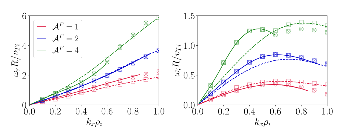
(a) Varying secondary mode wavenumber $k_{x}\rho_{i}$ at fixed $\delta=0$.

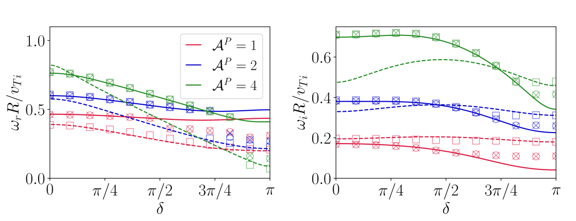
(b) Varying phase shift $\delta$ at fixed $k_{x}\rho_{i}=0.2$.

Figure 3: Secondary mode frequency (left) and growth rate (right) as a function of $k_{x}\rho_{i}$ (a) and $\delta$ (b) from the generalised secondary mode dispersion relation (31) (solid lines) and fastest growing mode from the ISM dispersion relation (30) (dashed lines) and from gyrokinetic simulations of the secondary mode (markers). Different primary amplitude values $\mathcal{A}^{P}$ (colors) are examined. The primary drive has the form (22) with $v_{Ex}^{P}\propto\sin(k_{y}^{P}y)$ and $\eta_{\perp}^{P}=\eta_{\parallel}^{P}=3\sin(k_{y}^{P}y+\delta)/\sin(k_{y}^{P}y)$. The primary drive varies along the magnetic field as $g_{i}^{P}\propto e^{-(\theta/\pi)^{2}}$. The gyrokinetic simulations of the secondary mode have a safety factor value $q=20$ and employ the phase-shift-periodic boundary condition (25) with $\Theta=0$ (circles) and $\Theta=0.288572618$ (crosses); the squares correspond to gyrokinetic simulations where the parallel streaming and binormal magnetic drift were artificially made to vanish. The three markers overlap in those cases where the secondary mode is unaffected by the choice of boundary condition and by the inclusion of in-surface derivatives.

The primary amplitude is seen in Figure 3(a) to strongly affect the growth rate of the TSM, which has a finite $\mathcal{A}^{P}$ threshold for instability. In contrast, increasing $\mathcal{A}^{P}$ causes smaller relative changes to the real frequency of the TSM, which approximately satisfies $\omega_{r}\approx 2k_{x}\rho_{i}v_{Ti}/R$, in agreement with Figure 1. The smaller relative changes in $\omega_{r}$ compared to $\omega_{i}$ with increasing $\mathcal{A}^{P}$ may also be observed in the TSM region of Figure 2(a). As shown in Figure 3(b), the frequency and growth rate of the TSM vary smoothly with the phase shift $\delta$ between the density and temperature of the primary drive. The TSM growth rate reaches its maximum for $\delta=0$ and its minimum for $\delta=\pi$, corresponding to the primary density and temperature gradient being parallel and anti-parallel, respectively. Given the relatively uninteresting dependence on the phase shift $\delta$, we will not consider finite phase shifts $\delta$ in the remainder of the simulations presented in this article, with $\eta_{\parallel}^{P}$ and $\eta_{\perp}^{P}$ chosen to be positive (negative) constants to model the parallel (anti-parallel) primary gradient cases. We note that this misses the peak of the ISM growth rate at $\delta=\pi/2$: the ISM, like the usual ITG primary mode, is destabilised by temperature gradients and stabilised by density gradients. The maximal ISM growth rate is therefore found at $\delta=\pi/2$, as there are then regions on the flux surface where the temperature gradient reaches its maximum while the density gradient vanishes.

In Figure 3, the toroidal secondary modes described by (31) become subdominant to the local ISMs (30) at small primary amplitudes $\mathcal{A}^{P}\lesssim 1$, at large wavenumbers $k_{x}\rho_{i}\gtrsim 1$ and at large phase shifts $\delta\sim\pi$. In these cases, the TSM complex frequency eventually enters the region of ISM complex frequencies (recall that $\mathcal{D}^{\mathrm{ISM}}=0$ gives a different complex frequency at each point on the flux surface because it depends on $y$ and $\theta$), as shown for example in Figure 4. For the TSM dispersion relation (31) to remain analytic, the integration contours corresponding to the flux-surface average $\langle 1/\mathcal{D}^{\mathrm{ISM}}\rangle_{\psi}$ must be deformed. Similarly to the case of Landau damping, the integral then has both a principal value and a pole contribution. In practice, numerically deforming the integration contour in (31) is cumbersome due to the presence of multiple poles and branch cuts. We therefore eschew such difficulties here, further motivated by the awareness that, as the TSM enters a region of ISMs, it necessarily becomes subdominant to a faster growing ISM (see also Figure 4). We thus capture the TSMs only up to the point where they enter the ISM region, whence the solid lines in Figure 3(a) do not extend to the largest values of $k_{x}\rho_{i}$. Note that only the fastest growing ISMs are captured in Figure 3, and the TSM will generally enter the ISM region at a smaller growth rate than the maximum ISM growth rate, see e.g. Figure 4.

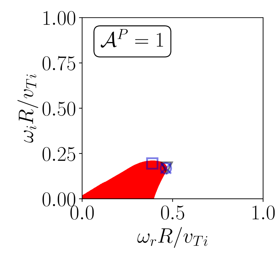
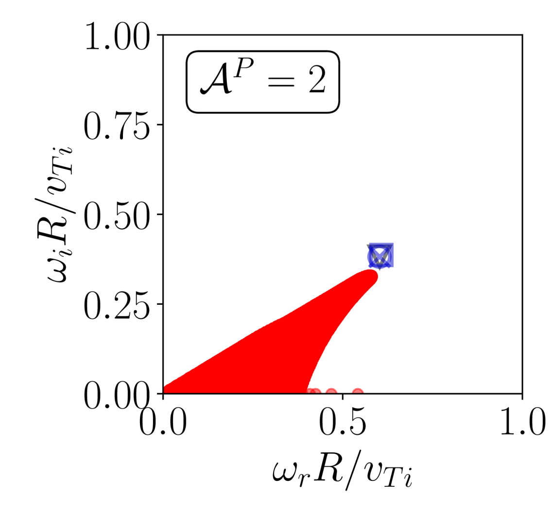
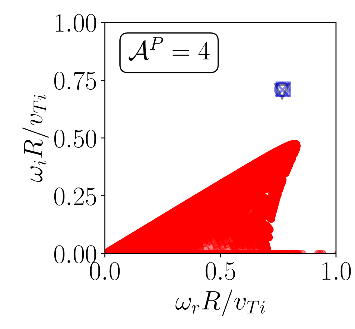
Figure 4: Real frequency and growth rate of ISMs for varying primary amplitudes $\mathcal{A}^{P}$ (left to right), with each red circle corresponding to the solution of (30) at a point on the flux surface. The simulations correspond to the $k_{x}\rho_{i}=0.2$ case in Figure 3(a), i.e. the primary drive varies as $g_{i}^{P}\propto e^{-(\theta/\pi)^{2}}$ and has $\eta_{\parallel}^{P}=\eta_{\perp}^{P}=3$. The TSM solution obtained from (31) is shown by the black triangle, while the mode frequencies from gyrokinetic simulations for a safety factor $q=20$ with phase shifts $\Theta=0$ and $\Theta=0.288572618$ are indicated by blue circles and crosses, respectively. The blue squares correspond to GK simulations with the parallel streaming and binormal magnetic drift set to zero.

3.2 ITG secondary modes (ISMs)

We now consider the ISMs described by (30). While the conventional ITG primary modes are driven unstable by a combination of the binormal magnetic drift and the background radial (temperature) gradient, the ISMs described by (30) are driven unstable by the radial magnetic drift and the primary binormal gradients. Indeed, the dispersion relation of a local toroidal ITG primary mode with binormal wavenumber $k_{y}$ is given by (30) with the replacements $b_{i}\rightarrow k_{y}^{2}\absolutevalue{\nabla y}^{2}\rho_{i}^{2}/2$ and

$$\mathcal{N}\rightarrow\frac{1}{n_{i}}\int\mathrm{d}^{3}v\,J_{0i}^{2}F_{Mi}\frac{k_{y}\tilde{v}_{My}-k_{y}\tilde{v}_{*i}}{\omega-k_{y}\tilde{v}_{My}}.$$ (35)

Here, $\tilde{v}_{My}=\tilde{\mathop{}\!\boldsymbol{v}}_{M}\cdot\nabla y$ is the binormal magnetic drift velocity and

$$\tilde{v}_{*i}\equiv\frac{T_{i}}{Z_{i}e}\frac{\boldsymbol{\hat{b}}\times\nabla x\cdot\nabla y}{B}\partial_{x}\ln n_{i}\left(1+\eta\left(\frac{v_{\parallel}^{2}+v_{\perp}^{2}}{v_{Ti}^{2}}-\frac{3}{2}\right)\right)\equiv v_{*i}\left(1+\eta\left(\frac{v_{\parallel}^{2}+v_{\perp}^{2}}{v_{Ti}^{2}}-\frac{3}{2}\right)\right)$$ (36)

is the ion diamagnetic velocity, with $\eta=\partial_{x}\ln T_{i}/\partial_{x}\ln n_{i}$.

The instability criterion of primary ITG modes is generally expressed in terms of $\eta$ and $v_{*i}\eta/v_{My}$. Instability requires $\eta(\eta-2/3)>0$ and $v_{*i}\eta/v_{My}$ to be sufficiently positive (see e.g. Biglari et al., 1989). Considering the case $\eta_{\parallel}^{P}=\eta_{\perp}^{P}=\eta^{P}$ for simplicity, these instability criteria translate directly to the ISMs. Their instability thus requires $\eta^{P}(\eta^{P}-2/3)>0$ and sufficiently large $\tau v_{Ex}^{P}\eta/v_{Mx}$. The latter criterion is generally easily satisfied for any finite $\mathcal{A}^{P}$ at certain points on the flux surface, as there are always points with $v_{Mx}=0$, e.g. at $\theta\in\{0,\pi\}$ in a circular cross-section tokamak for which $v_{Mx}\propto\sin\theta$.

In contrast, the TSM’s instability threshold is at a finite $\mathcal{A}^{P}$, as discussed in Section 3.3. Therefore, the theory predicts a region of unstable ISMs and stable TSMs at weak primary drive. At sufficiently large primary drive and moderate radial wavelengths $k_{x}\rho_{i}\lesssim 1$, the TSM grows faster than the ISMs, see Figure 3(a). This will be explained further in Section 3.4, where the non-resonant limit of the dispersion relations (30) and (31) is considered. Even at large primary drive, the ISM generally remains the dominant instability at short wavelengths $k_{x}\rho_{i}\gtrsim 1$. While a full theoretical analysis is beyond the scope of this study, this result may be understood qualitatively by noting that ITG primary modes typically remain unstable even at wavelengths shorter than the ion gyroradius (Smolyakov et al., 2002; Gao et al., 2005), while the RDK secondary mode (towards which the secondary mode tends at large primary amplitude, see Section 3.4) is generally stabilised at short wavelengths by FLR effects, see B. Therefore, for large $\mathcal{A}^{P}$, the ISM should be the dominant instability at short radial wavelengths; however, its growth rate will typically be smaller than that of the RDK secondary mode at long radial wavelengths, see e.g. Figure 2(a).

3.3 Toroidal secondary modes (TSMs)

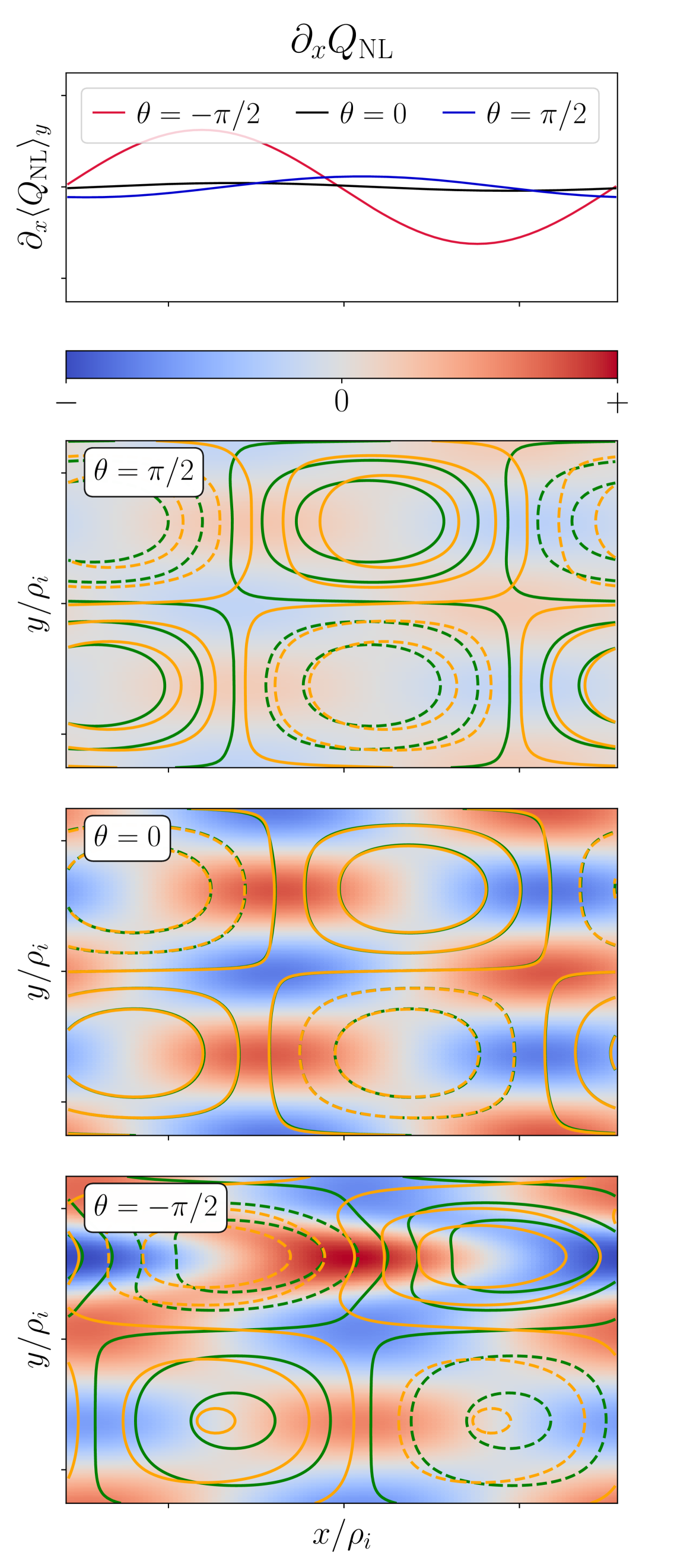
(a) $\mathcal{A}^{P}=4$

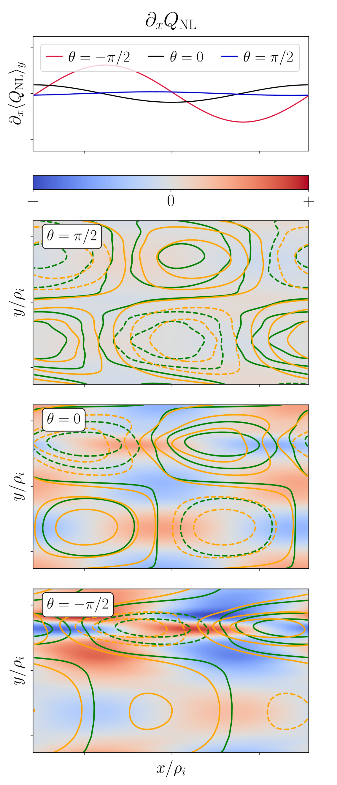
(b) $\mathcal{A}^{P}=1$

Figure 5: Spatial variation of the nonlinear contribution $\partial_{x}Q_{\mathrm{NL}}$ (39) to the SW force evolution (43) in the toroidal secondary mode simulations presented in Figure 3(a) for $\mathcal{A}^{P}=4$ (left column) and $\mathcal{A}^{P}=1$ (right column) at $k_{x}\rho_{i}=0.1$. The $y$-integrated value of $\partial_{x}Q_{\mathrm{NL}}$ is shown in the top row as a function of $x$ for three values of $\theta\in\{\pi/2,0,-\pi/2\}$ (above, on, and below the tokamak midplane, respectively). The second, third, and fourth rows show the variation of $\partial_{x}Q_{\mathrm{NL}}$ in $(x,y)$ for these three $\theta$ values, as well as contours of the nonzonal pressure fluctuations $P^{\mathrm{NZ}}$ (orange contours) and electrostatic potential fluctuations $\varphi^{\mathrm{NZ}}$ (green contours), with negative values indicated by dashed lines. For $\mathcal{A}^{P}=4$, the $P^{\mathrm{NZ}}$ and $\varphi^{\mathrm{NZ}}$ contours are overlapping at $\theta=0$, and have phase shifts of opposite signs at $\theta=\pm\pi/2$ due to the radial magnetic drift advection. Moreover, the inward-propagating ($\omega/k_{x}<0$) TSM shown here is strongly localised to $\theta=-\pi/2$. As a result, $\langle\partial_{x}Q_{\mathrm{NL}}\rangle_{y}$ has a large up-down asymmetry, see first row. In the $\mathcal{A}^{P}=1$ case, $\partial_{x}Q_{\mathrm{NL}}$ exhibits contributions from higher $y$-harmonics, but its $y$-averaged value still has a similar up-down asymmetry.

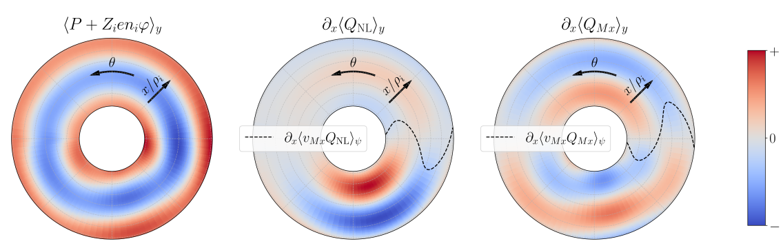
(a) $\mathcal{A}^{P}=4$

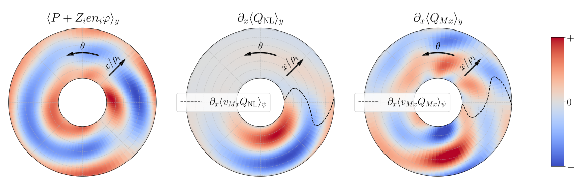
(b) $\mathcal{A}^{P}=1$

Figure 6: Contour plots in $x$ and $\theta$ of integrand in SW force (left plots), whose time evolution (43) results from the nonlinear term (39) (middle plots) and the magnetic drift term (44) (right plots). The contours correspond to the simulations presented in Figure 3(a) for $k_{x}\rho_{i}=0.1$, $\mathcal{A}^{P}=4$ (top row) and $\mathcal{A}^{P}=1$ (bottom row). The contributions to the time evolution of the SW force on each flux surface, $\partial_{x}\langle v_{Mx}Q_{\mathrm{NL}}\rangle_{\psi}(x)$ and $\partial_{x}\langle v_{Mx}Q_{Mx}\rangle_{\psi}(x)$, are indicated by black dashed lines on the outboard midplane in the middle and right plots, respectively. These two contributions cancel out, such that $\langle P+Z_{i}en_{i}\varphi\rangle_{y}$ has no up-down asymmetric component (left plots), i.e. $\langle v_{Mx}(P+Z_{i}en_{i}\varphi)\rangle_{\psi}\approx 0$.

We proceed to discuss the physics of the toroidal secondary modes in more detail. We first investigate whether the basic physical picture of the TSM put forward in Nies et al. (2024) is consistent with the GK simulations. The main argument is reproduced here, considering for simplicity a tokamak with circular flux surfaces, where the radial magnetic drift velocity $\tilde{v}_{Mx}\propto\sin\theta$ is up-down asymmetric. We define the pressure-like quantity

$$P=T_{i}\int\mathrm{d}^{3}v\,\frac{v_{\parallel}^{2}+v_{\perp}^{2}/2}{v_{Ti}^{2}}g_{i}.$$ (37)

Note the factor of two between the parallel and perpendicular velocity contributions, which reflects the velocity dependence of the radial magnetic drift (10). The TSM relies on the Stringer-Winsor (SW) force in the vorticity equation (9), which arises due to up-down asymmetry in $\langle P+Z_{i}en_{i}\varphi\rangle_{y}$. By multiplying the GK equation (1) by $\tilde{v}_{Mx}$, integrating in velocity space, and flux-surface averaging, we find that, at long perpendicular wavelengths, the pressure contribution to the SW force evolves in time as

$$\partial_{t}\langle v_{Mx}P\rangle_{\psi}=T_{i}\left\langle\int\mathrm{d}^{3}v\,\tilde{v}_{Mx}\,\partial_{t}g_{i}\right\rangle_{\psi}=-\partial_{x}\left\langle v_{Mx}\left(Q_{\mathrm{NL}}+Q_{Mx,P}\right)\right\rangle_{\psi}.$$ (38)

Here, the contribution from the nonlinear turbulent heat flux is given by

$$Q_{\mathrm{NL}}=T_{i}v_{Ex}\int\mathrm{d}^{3}v\,\frac{v_{\parallel}^{2}+v_{\perp}^{2}/2}{v_{Ti}^{2}}g_{i},$$ (39)

and the contribution from the radial magnetic drift is

$$Q_{Mx,P}=v_{Mx}\left(\frac{7}{4}n_{i}Z_{i}e\varphi+T_{i}\int\mathrm{d}^{3}v\,\left(\frac{v_{\parallel}^{2}+v_{\perp}^{2}/2}{v_{Ti}^{2}}\right)^{2}g_{i}\right).$$ (40)

To obtain (38), we have neglected the contributions from binormal derivatives and parallel streaming, as befits the assumptions made in deriving the dispersion relation of toroidal secondary modes (30). We have also neglected FLR effects to simplify the discussion. The derived time evolution equation does not include the effect of the $\theta$-varying potential on the SW force. To calculate this piece, we evaluate the time derivative of the quasineutrality equation (8), which after flux-surface averaging gives

$$\partial_{t}\langle v_{Mx}Z_{i}en_{i}\varphi\rangle_{\psi}=\frac{T_{i}}{\tau}\left\langle v_{Mx}\int\mathrm{d}^{3}v\,\partial_{t}g_{i}\right\rangle_{\psi}=-\partial_{x}\left\langle v_{Mx}\,Q_{Mx,\varphi}\right\rangle_{\psi},$$ (41)

with

$$Q_{Mx,\varphi}=\frac{v_{Mx}}{\tau}\left(n_{i}Z_{i}e\varphi+T_{i}\int\mathrm{d}^{3}v\,\frac{v_{\parallel}^{2}+v_{\perp}^{2}/2}{v_{Ti}^{2}}g_{i}\right).$$ (42)

In deriving (41), we have again neglected the effects of parallel streaming and FLR effects. By combining (38) and (41), the time derivative of the SW force is derived to be

$$\partial_{t}\langle v_{Mx}\left(P+Z_{i}en_{i}\varphi\right)\rangle_{\psi}=-\partial_{x}\left\langle v_{Mx}\left(Q_{\mathrm{NL}}+Q_{Mx}\right)\right\rangle_{\psi},$$ (43)

with $Q_{\mathrm{NL}}$ given by (39) and $Q_{Mx}$ by

$$Q_{Mx}=Q_{Mx,P}+Q_{Mx,\varphi}.$$ (44)

The physical mechanism behind the TSM may be understood qualitatively as follows. The zonal flow shears the (primary) background turbulence to small radial scales. The radial magnetic drift’s velocity dependence ($\tilde{v}_{Mx}\propto v_{\parallel}^{2}+v_{\perp}^{2}/2$) then causes a phase shift between the sheared potential and pressure fluctuations, as they are advected at different rates in the $x$-direction. This phase shift leads to an up-down asymmetric $\langle Q_{\mathrm{NL}}\rangle_{y}\propto\langle P\partial_{y}\varphi\rangle_{y}$ (as the phase shift is caused by $\tilde{v}_{Mx}\propto\sin\theta$) and thence a contribution to the SW force. The up-down asymmetric phase shift between potential and pressure fluctuations in GK simulations of the TSM is shown in Figure 5, alongside the resulting $Q_{\mathrm{NL}}$.

If the ZF inertia in (9) is negligible (as is the case at long radial wavelengths $k_{x}\rho_{i}\lesssim 0.5$), the ZF amplitude quickly adjusts to ensure the $Q_{Mx}$ contribution to the SW force evolution (43) cancels that from $Q_{\mathrm{NL}}$. The cancellation between $Q_{\mathrm{NL}}$ and $Q_{Mx}$ is indeed observed in GK simulations of the toroidal secondary mode at long radial wavelengths, as shown in Figure 6.

The cancellation is predicated on the smallness of the inertia and nonlinear stress contributions to the vorticity equation (9), which need not be small for $k_{x}\rho_{i}\sim 0.5$, the scale at which the toroidal secondary mode amplitude peaks in turbulence simulations, see Figure 1. The Stringer-Winsor force can then synergise or compete with the ZF inertia and the nonlinear stresses - such effects are captured by the dispersion relation (31) and will be discussed below when considering its non-resonant limit (49).

The mode propagates radially with a speed approximately equal to the magnetic drift velocity $\omega/k_{x}\sim v_{Mx}(\theta=\pm\pi/2)$ due to the role of the radial magnetic drift in generating the up-down asymmetric $Q_{\mathrm{NL}}$. The TSM is thus subject to kinetic damping by the magnetic drifts and requires a sufficiently large primary drive to become unstable, typically $\mathcal{A}^{P}\gtrsim 1$, depending on other parameters such as $\eta_{\parallel}^{P}$ and $\eta_{\perp}^{P}$.

The inward-propagating TSMs ($\omega/k_{x}<0$) considered in Figures 5 and 6 have $\partial_{x}\langle Q_{\mathrm{NL}}\rangle_{y}$ strongly localised below the midplane ($\theta=-\pi/2$). This localisation follows from the denominator in (27), with particle resonances being dominant when the signs of the real frequency $\omega_{r}$ and of the magnetic drift frequency $k_{x}v_{Mx}$ are identical. For $\mathcal{A}^{P}=4$, the radial magnetic drift contribution $\partial_{x}\langle Q_{Mx}\rangle_{y}$ dominantly varies as $\sin\theta$, which follows from the first terms in (40) and (42) being dominant, and $\langle\varphi\rangle_{y}$ being approximately constant along the magnetic field in this case (see also the non-resonant limit in Section 3.4). For $\mathcal{A}^{P}=1$, $\partial_{x}\langle Q_{Mx}\rangle_{y}$ still has a dominant $\sin\theta$-variation but also exhibits higher $\theta$-harmonics.

Finally, we note the physical mechanism presented above does not strongly depend on the phase shift between the primary potential and pressure perturbations, as may be seen from Figure 3(b). While this phase shift strongly affects the total ($x$-integrated) nonlinear heat flux $Q_{\mathrm{NL}}$, it does not contribute to the SW force which requires a radial modulation of $\partial_{x}Q_{\mathrm{NL}}$.

3.4 Non-resonant limit of secondary modes

The following study of the non-resonant limit is primarily motivated by the aspiration to identify the various modes described by (31). If the primary amplitude is sufficiently large, the effect of the radial magnetic drift should become subdominant and we expect to recover the purely growing RDK secondary mode (Rogers et al., 2000). Moreover, when the primary amplitude vanishes, we expect to recover GAMs from (31). The non-resonant limit of (31) will help understand under which conditions the various modes described by the dispersion relation become dominant. Furthermore, by also considering the non-resonant limit of the ISM dispersion relation, we will be able to explain why the ISM becomes subdominant to the TSM for sufficiently large $\mathcal{A}^{P}$ (see Figure 3(a)).

We consider the subsidiary ordering

$$b_{i}^{1/2}\sim\frac{k_{x}\tilde{v}_{Mx}}{\omega}\ll\frac{k_{x}\tilde{v}_{g}^{P}}{\omega}\sim\frac{k_{x}v_{Ex}^{P}}{\omega}\sim\tau\sim 1,$$ (45)

corresponding to a regime where the secondary mode is strongly driven and the FLR effects are weak. For convenience, we define some velocities associated with various moments of the primary distribution $g_{i}^{P}$, first that corresponding to the primary diamagnetic momentum

$$v_{\mathrm{dia}}^{P}=\frac{1}{n_{i}}\int\mathrm{d}^{3}v\,F_{Mi}\tilde{v}_{g}^{P}\frac{v_{\perp}^{2}}{v_{Ti}^{2}},$$ (46)

and secondly those moments associated with powers of the magnetic drift velocity $\tilde{v}_{Mx}$ (10)

$$v_{j}^{P}=\frac{1}{n_{i}}\int\mathrm{d}^{3}v\,F_{Mi}\tilde{v}_{g}^{P}\left(\frac{v_{\parallel}^{2}+v_{\perp}^{2}/2}{v_{Ti}^{2}}\right)^{j},$$ (47)

with $v_{0}^{P}=\tau v_{Ex}^{P}$ due to quasineutrality (8) in the assumed limit of large binormal scales $k_{y}^{P}\rho_{i}\ll 1$. Furthermore, we assume here and in the rest of this paper that the primary distribution satisfies

$$\langle\tilde{v}_{Mx}f(g_{i}^{P})\rangle_{\theta}=0$$ (48)

for an arbitrary function $f(g_{i}^{P})$. In a tokamak with flux surfaces of circular cross-section where $\tilde{v}_{Mx}\propto\sin\theta$, this corresponds to the requirement that the primary drive has no up-down asymmetry. If one considered primary distributions violating condition (48), one would preimpose the up-down asymmetry required for the SW force. Instead, the toroidal secondary mode mechanism self-consistently generates the up-down pressure asymmetry from an up-down symmetric primary drive, as explained in Nies et al. (2024) and Section 3.3.

The non-resonant limit of the generalised secondary mode dispersion relation (31) corresponding to the ordering (45) may be written as

$$0=\mathcal{D}^{\mathrm{NR}}=\frac{1}{\tau}\left\langle b_{i}+b_{i}k_{x}^{2}\frac{v_{Ex}^{P}\left(v_{Ex}^{P}+v_{\mathrm{dia}}^{P}\right)}{\omega^{2}}-\left(\frac{k_{x}v_{Mx}}{\omega}\right)^{2}\left[\frac{7}{4}+\frac{1}{\tau}+\frac{(k_{x}v_{1}^{P})^{2}/(\tau\omega)-k_{x}v_{2}^{P}}{\omega-k_{x}v_{Ex}^{P}}\right]\right\rangle_{\psi}.$$ (49)

This result may be obtained by expanding (31). First, we exploit the smallness of the radial magnetic drift to expand the resonant denominator in (29). Then, also using $b_{i}\ll 1$, the denominator in the flux-surface average (31) is expanded. Finally, many terms vanish due to $\langle v_{Ex}^{P}\rangle_{y}=0$, $\langle v_{\mathrm{dia}}^{P}\rangle_{y}=0$, and assumption (48), leading to (49). An alternative derivation of (49) from the vorticity equation (9) may be found in A, where the growth of secondary modes in the limit of strong drive and long perpendicular wavelengths is considered more generally.

The contributions to (49) may directly be associated to terms in the vorticity equation (9): the first two terms originate from the ZF inertia and the nonlinear stresses, which is composed of the Reynolds stress (the $(v_{Ex}^{P})^{2}$ term) and the diamagnetic stress (the $v_{Ex}^{P}v_{\mathrm{dia}}^{P}$ term). The $v_{Mx}$ contribution in (49) stems from the SW force, whose time evolution (43) has contributions from $Q_{\mathrm{NL}}$ and $Q_{Mx}$, given by (39) and (44), respectively. With the ordering (45), only the first terms in (40) and (42) contribute to $Q_{Mx}$, giving the linear term ($\propto 7/4+1/\tau$) in (49). Finally, up-down asymmetries of $v_{Ex}$ and of $g_{i}$ in (39) cause the $v_{1}^{P}$ and $v_{2}^{P}$ terms in (49), respectively.

The non-resonant dispersion relation (49) lays bare the different modes contained in the more general dispersion relation (31). First, in the limit of vanishing primary drive, the balance of ZF inertia and the linear contribution to the SW force in (49) recovers the GAM (Winsor et al., 1968; Conway et al., 2021) dispersion relation

$$\omega_{\mathrm{GAM}}^{2}=\left(\frac{7}{4}+\frac{1}{\tau}\right)\frac{\langle(k_{x}v_{Mx})^{2}\rangle_{\psi}}{\langle b_{i}\rangle_{\psi}}.$$ (50)

Second, in the limit of vanishing radial magnetic drift, the RDK dispersion relation (Rogers et al., 2000; Plunk and Navarro, 2017) is recovered from the balance of ZF inertia and nonlinear stresses,

$$\omega_{\mathrm{RDK}}^{2}=-k_{x}^{2}\frac{\left\langle b_{i}\,v_{Ex}^{P}\left(v_{Ex}^{P}+v_{\mathrm{dia}}^{P}\right)\right\rangle_{\psi}}{\left\langle b_{i}\right\rangle_{\psi}},$$ (51)

giving a purely growing mode when the right-hand-side is negative. We may now deduce from (49) that the RDK secondary mode is recovered strictly only in the limit $\omega_{\mathrm{RDK}}^{2}\sim(k_{x}v_{Ex}^{P})^{2}\gg(k_{x}v_{Mx})^{2}/b_{i}\sim\omega_{\mathrm{GAM}}^{2}$. In practice, the saturated turbulence amplitude does not reach such large values, so that the effect of the radial magnetic drift on the secondary modes must be considered. Indeed, the toroidal secondary modes are clearly observed in GK simulations of ITG turbulence, see Figure 1.

Finally, the non-resonant limit of the toroidal secondary mode is contained in (49) through the nonlinear contributions to the SW force from the $v_{1}^{P}$ and $v_{2}^{P}$ terms. To evaluate the non-resonant limit of the TSM, we consider a simplified primary drive that is described by a single Fourier mode in $y$ and is independent of $\theta$, such that $v_{Ex}^{P}=v_{Ex}^{P0}\sin(k_{y}^{P}y)$, $v_{\mathrm{dia}}^{P}=v_{\mathrm{dia}}^{P0}\sin(k_{y}^{P}y)$, $v_{1}^{P}=v_{1}^{P0}\sin(k_{y}^{P}y)$, and $v_{2}^{P}=v_{2}^{P0}\sin(k_{y}^{P}y)$. We thus exclude here for simplicity any variation of the primary drive along the magnetic field and the possibility of a phase shift between various moments of the primary distribution. The non-resonant dispersion relation (49) simplifies to

$$0=1+\left(\frac{k_{x}v_{Ex}^{P0}}{\omega}\right)^{2}C_{\mathrm{RDK}}-\frac{\omega_{\mathrm{GAM}}^{2}}{\omega^{2}}\left[1-C_{\mathrm{TSM}}\left(1-\frac{1}{\sqrt{1-\left(k_{x}v_{Ex}^{P0}/\omega\right)^{2}}}\right)\right],$$ (52)

where we used the integral (101). Here, the square root is evaluated with the branch cut along negative reals, such that Re$\sqrt{x}>0$. We have defined

$$C_{\mathrm{RDK}} =\frac{1}{2}\left(1+\frac{v_{\mathrm{dia}}^{P0}}{v_{Ex}^{P0}}\right),$$ (53)

$$C_{\mathrm{TSM}} =\left(\frac{7}{4}+\frac{1}{\tau}\right)^{-1}\left(\frac{1}{\tau}\left(\frac{v_{1}^{P0}}{v_{Ex}^{P0}}\right)^{2}-\frac{v_{2}^{P0}}{v_{Ex}^{P0}}\right).$$ (54)

We may rewrite (52) as an equation for $k_{x}v_{Ex}^{P0}/\omega$,

$$\frac{1}{\sqrt{1-\left(k_{x}v_{Ex}^{P0}/\omega\right)^{2}}}=\frac{C_{1}}{\left(k_{x}v_{Ex}^{P0}/\omega\right)^{2}}+\frac{C_{2}}{C_{1}},$$ (55)

with real parameters

$$C_{1}=\frac{1}{C_{\mathrm{TSM}}}\left(\frac{k_{x}v_{Ex}^{P0}}{\omega_{\mathrm{GAM}}}\right)^{2}$$ (56)

and

$$C_{2}=\frac{1}{C_{\mathrm{TSM}}^{2}}\left(\frac{k_{x}v_{Ex}^{P0}}{\omega_{\mathrm{GAM}}}\right)^{2}\left[C_{\mathrm{RDK}}\left(\frac{k_{x}v_{Ex}^{P0}}{\omega_{\mathrm{GAM}}}\right)^{2}+C_{\mathrm{TSM}}-1\right].$$ (57)

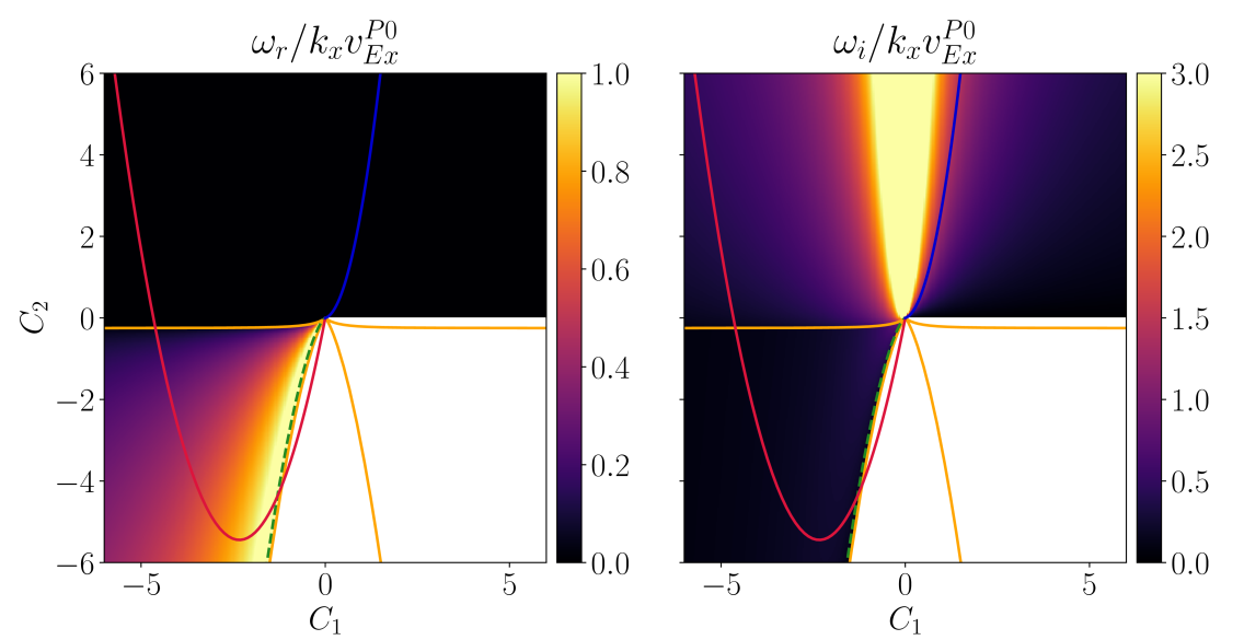
(a) Real frequency (left) and growth rate (right) of fastest growing mode from non-resonant secondary mode dispersion relation for a single Fourier mode primary drive (55). The blank region has no unstable modes. The orange lines correspond to the zeroes of the discriminant (58). The green-dashed line is the approximation (59) to the curve bounding the stable region. The red and blue curves correspond to the $C_{1}$ and $C_{2}$ values in the primary amplitude scan of (b).

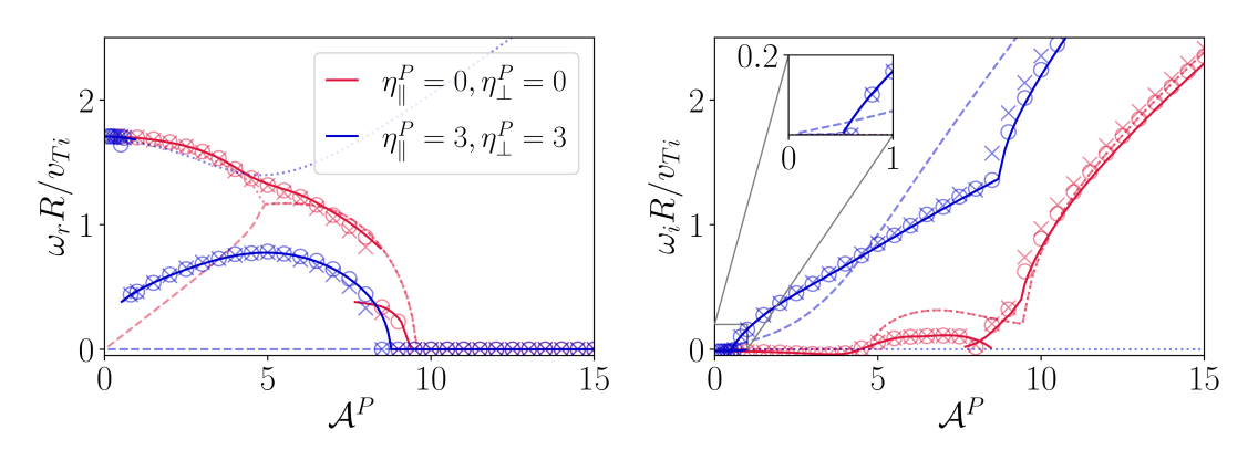
(b) Real frequency (left) and growth rate (right) for $k_{x}\rho_{i}=0.2$ as a function of the primary amplitude $\mathcal{A}^{P}$ from generalised secondary mode dispersion relation (31) (solid lines), gyrokinetic simulations of the secondary modes (markers), and from non-resonant limit of the dispersion relation (52) (dashed and dotted lines). The primary drive is here taken to be constant in $\theta$ and two sets of $\eta_{\parallel,\perp}^{P}$ values are considered (red and blue colors). The gyrokinetic simulations of the secondary modes have a safety factor value $q=20$ and employ the phase-shift-periodic boundary condition (25) with $\Theta=0$ (circles) and $\Theta=0.28857261$ (crosses).

Figure 7: Parameter space of non-resonant secondary modes (top) and comparison with general secondary mode theory and gyrokinetic simulations (bottom).

The solutions to (55) are shown in Figure 7(a). The stable region is bounded by two curves, the first is given by the line $\{C_{2}=0,C_{1}\geq 0\}$ and the second is determined as a root of

$$0=\Delta=4C_{2}(C_{1}^{2}+C_{2})^{3}+C_{1}^{2}(C_{1}^{4}+4C_{1}^{2}+20C_{2}C_{1}^{2}-8C_{2}^{2}).$$ (58)

Here, $\Delta$ is the discriminant of the cubic equation obtained by squaring and rearranging (55). An approximate solution to the nontrivial curve bounding the stable region is given by

$$C_{2}\approx C_{1}\left(-C_{1}+3\left(-\frac{C_{1}}{4}\right)^{1/3}\right).$$ (59)

This expression is strictly valid for $-C_{1}\gg 1$ but is shown in Figure 7(a) to be a good approximation for all $C_{1}$.

As shown in Figure 7(a), the non-resonant secondary mode dispersion (49) describes both purely growing instabilities and overstable modes with $\omega_{r}\neq 0$ and $\omega_{i}>0$. The former are found approximately in the region $C_{2}>0$ which by (57) is equivalent to $C_{\mathrm{RDK}}>0$ for large primary amplitudes $k_{x}v_{Ex}^{P0}\gg\omega_{\mathrm{GAM}}$, and to $C_{\mathrm{TSM}}>1$ for small primary amplitudes. These correspond to the RDK secondary mode and non-resonant TSM, respectively. A necessary condition for overstability is $C_{1}<0$, which is equivalent by (56) to $C_{\mathrm{TSM}}<0$, which may be interpreted as the nonlinearly induced up-down pressure asymmetry (39) reinforcing that from the radial magnetic drift (44).

The non-resonant secondary mode solutions from (52) are shown in Figure 7(b) to agree with the solutions of the resonant dispersion relation (31) and with GK simulation results at large primary amplitudes $\mathcal{A}^{P}\gg 1$, while both qualitative and quantitative deviations are generally observed for $\mathcal{A}^{P}\sim 1$. When the primary mode is taken to be a pure density perturbation ($\eta_{\parallel}^{P}=\eta_{\perp}^{P}=0$), the non-resonant limit describes qualitatively how the initially stable GAM first becomes overstable at $\mathcal{A}^{P}\approx 5$, and then becomes a purely growing mode at $\mathcal{A}^{P}\approx 10$, see also trajectory in $(C_{1},C_{2})$-space in Figure 7(a). However, for the $\eta_{\parallel}^{P}=\eta_{\perp}^{P}=3$ case, the non-resonant solution cannot capture the kinetic nature of the toroidal secondary mode for $\mathcal{A}^{P}\lesssim 10$. Indeed, it fails to reproduce the finite real frequency of the toroidal secondary mode for $\mathcal{A}^{P}\lesssim 10$, as $\omega_{r}\sim k_{x}v_{Mx}$ is neglected in the ordering (45). Neither does the non-resonant dispersion relation capture the threshold in the primary amplitude for instability, as shown by the inset in Figure 7(b).

The coefficients $C_{\mathrm{RDK}}$ (53) and $C_{\mathrm{TSM}}$ (54) may be evaluated for the model primary distribution function (22) to be

$$C_{\mathrm{RDK}} =\frac{1}{2}\left(1+\tau(1+\eta_{\perp}^{P})\right),$$ (60)

$$C_{\mathrm{TSM}} =\tau\left(\frac{7}{4}+\frac{1}{\tau}\right)^{-1}\left(\left(1+\frac{\eta_{\parallel}^{P}+\eta_{\perp}^{P}}{2}\right)^{2}-\left(\frac{7}{4}+2\eta_{\parallel}^{P}+\frac{3\eta_{\perp}^{P}}{2}\right)\right).$$ (61)

The RDK secondary mode requires $C_{\mathrm{RDK}}>0$, i.e. $\eta_{\perp}^{P}$ cannot be too negative, otherwise the diamagnetic stress opposes the Reynolds stress too strongly. The coefficient $C_{\mathrm{TSM}}$ is negative for $\eta_{\parallel}^{P},\eta_{\perp}^{P}\rightarrow 0$ and positive at large $\absolutevalue{\eta_{\parallel}^{P}+\eta_{\perp}^{P}}$, explaining the differences between the pure density and $\eta_{\parallel}^{P}=\eta_{\perp}^{P}=3$ cases in Figure 7.

The stability of secondary modes as a function of $\eta_{\parallel}^{P}$ and $\eta_{\perp}^{P}$ for various primary amplitudes is studied in Figure 8. The stability limits obtained from the non-resonant dispersion relation are shown therein to approximate those obtained from GK simulations. Although discrepancies are observed at small $\mathcal{A}^{P}\sim 1$, the non-resonant limit still qualitatively reproduces the stability boundary, i.e. instability at large $\absolutevalue{\eta_{\parallel}^{P}+\eta_{\perp}^{P}}$. The non-resonant limit also correctly captures the region of overstable solutions, see e.g. green curve for $\mathcal{A}_{P}=16$ in Figure 8.

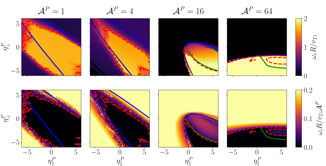
Figure 8: Real frequency (top row) and growth rate normalised by $\mathcal{A}^{P}$ (bottom row) at $k_{x}\rho_{i}=0.1$ from gyrokinetic simulations for a model primary distribution function (22) constant in $\theta$, with different values of $\eta_{\parallel}^{P}$ and $\eta_{\perp}^{P}$ and four primary amplitude values $\mathcal{A}^{P}$ (left to right). A safety factor value $q=20$ is chosen and the phase-shift-periodic boundary condition (25) with $\Theta=0$ is used. Due to computational cost, the simulations are performed with a reduced resolution $\{N_{y},N_{\theta},N_{v_{\parallel}},N_{\mu}\}=\{4,24,32,8\}$. The transitions from stable to purely growing modes ($\omega_{r}=0$) and from stable to overstable modes ($\omega_{r}\neq 0$) given by the non-resonant dispersion (52) are indicated by blue and green lines, respectively. The numerically determined instability threshold is indicated by red dashed lines.

Finally, we investigate the conditions under which the ISM dominates over the TSM and RDK secondary mode in the non-resonant limit. Just like for the usual ITG primary mode, a non-resonant dispersion relation for the ISM may be found by considering a large driving temperature gradient compared to the density gradient, i.e. $\eta_{\parallel}^{P},\eta_{\perp}^{P}\gg 1$. We thus consider the ordering $b^{1/2}\sim k_{x}v_{Mx}\ll\omega\sim k_{x}v_{Ex}^{P}\ll\eta_{\parallel}^{P}k_{x}v_{Ex}^{P}\sim\eta_{\perp}^{P}k_{x}v_{Ex}^{P}$. The ISM dispersion relation (30) then simplifies to

$$0=\mathcal{D}^{\mathrm{ISM,NR}}=\frac{1}{(\omega-k_{x}v_{Ex}^{P})^{2}}\left(\tau\omega(\omega-k_{x}v_{Ex}^{P})+k_{x}^{2}v_{Mx}v_{1}^{P}\right),$$ (62)

with roots

$$\omega_{\mathrm{ISM,NR}}=\frac{1}{2}k_{x}\left(v_{Ex}^{P}\pm\sqrt{(v_{Ex}^{P})^{2}-4v_{Mx}v_{1}^{P}/\tau}\right).$$ (63)

In this limit, the ISM is unstable when the argument of the square root is negative, i.e. for large $\absolutevalue{v_{1}^{P}}$ and $v_{1}^{P}v_{Mx}>0$ (corresponding to ‘bad curvature’). Its growth rate is bounded by Im$(\omega_{\mathrm{ISM}})\leq k_{x}\sqrt{\absolutevalue{v_{Mx}v_{1}^{P}}/\tau}$, i.e. the bound on the growth rate scales with the square root of the primary temperature gradient. At large $\mathcal{A}^{P}$ (and/or large $\eta_{\parallel}^{P},\eta_{\perp}^{P}$), the ISM will thus be subdominant to the RDK secondary mode and the TSM, whose growth rates increase linearly with the primary gradients.

3.5 Secondary modes with finite binormal wavenumber and parallel streaming

The theory of secondary modes in toroidal geometry presented above assumed small binormal wavenumbers and parallel streaming, which allowed us to simplify the GK equation (11) to an algebraic equation (26), leading to the dispersion relations (30) and (31). In this section, the limits of validity of these assumptions are studied. First, the effects of finite binormal wavenumbers are studied numerically in Section 3.5.1. Then, the effects of parallel streaming on the TSM and RDK secondary mode are considered in Section 3.5.2.

We note that the GK simulations of the secondary mode still enforce the primary drive to be constant in time, an assumption which may become unjustified as the binormal drifts and parallel streaming are sufficiently increased. For example, the results presented here may overemphasise the role of binormal drifts and parallel streaming as the simulations will exaggerate the frequency mismatch between the primary drive and the secondary mode, which has previously been found to stabilise secondary instabilities (Chen et al., 2000).

3.5.1 Binormal drifts and magnetic shear effects

In Figure 9, gyrokinetic simulations of secondary modes are shown for various binormal wavenumbers of the primary mode. Both the usual magnetic shear value $\hat{s}=0.8$ and a smaller value $\hat{s}=0.01$ are considered. A case with artificially removed binormal drifts is also included to separate the potential stabilisation due to FLR effects from the stabilisation due to the binormal component of the magnetic drift.

We remind the reader that the magnetic shear $\hat{s}$ enters $\nabla y$ and therefore affects both the binormal magnetic drift $\mathop{}\!\boldsymbol{\tilde{v}}_{M}\cdot\nabla y$ and the strength of the FLR effects through $k_{\perp}^{2}=k_{x}^{2}\absolutevalue{\nabla x}^{2}+2k_{x}k_{y}\nabla x\cdot\nabla y+k_{y}^{2}\absolutevalue{\nabla y}^{2}$. In a large aspect ratio tokamak with circular flux surfaces, the binormal magnetic drift’s variation along the magnetic field is approximately $\mathop{}\!\boldsymbol{\tilde{v}}_{M}\cdot\nabla y\propto\cos\theta+\hat{s}\theta\sin\theta$. Therefore, for larger $\hat{s}$, the strength of the binormal magnetic drift at $\theta\sim\pm\pi/2$ is substantially increased, and it should be expected to affect the TSM more strongly.

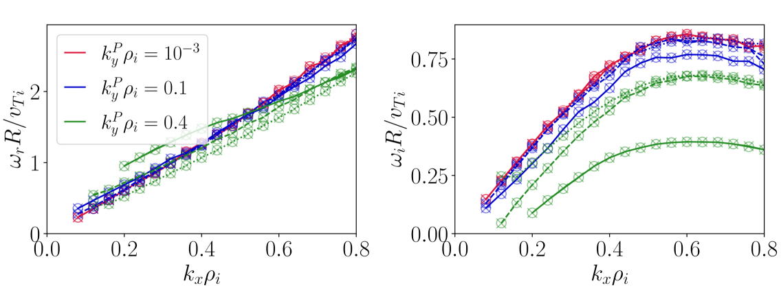
Figure 9: Secondary mode frequency (left) and growth rate (right) from gyrokinetic simulations of secondary modes for varying primary binormal wavenumbers $k_{y}^{P}$ (colors) and magnetic shear values $\hat{s}=0.8$ (solid lines) and $\hat{s}=0.01$ (dashed lines). A case with $\hat{s}=0.8$ and with binormal magnetic drifts artificially removed in the simulations is also included (dotted lines). The phase-shift factors $\Theta=0$ (circles) and $\Theta=0.288572618$ (crosses) are considered. The primary distribution has the form (22) with $\eta_{\perp}^{P}=\eta_{\parallel}^{P}=3$, amplitude $\mathcal{A}^{P}=2$, and it varies along the magnetic field as $g_{i}^{P}\propto e^{-(\theta/\pi)^{2}}$. A safety factor value $q=20$ is used.

Indeed, Figure 9 shows that increasing the primary binormal wavenumber affects the TSM growth rate most strongly through the binormal component of the magnetic drift at sufficiently large magnetic shear (solid lines). In comparison, the reduction in the peak TSM growth rate is modest in the cases where the magnetic shear is small (dashed lines) or the binormal component of the magnetic drift is zeroed out (dotted lines). For smaller $k_{x}\rho_{i}$, the binormal magnetic drift stabilises the TSM independently of the value of the magnetic shear (dashed and solid lines), bringing about a noticeable threshold in $k_{x}\rho_{i}$ for instability. We note that the stabilisation of the TSM by binormal magnetic drifts and FLR effects in Figure 9 requires large $k_{y}^{P}\rho_{i}$, as it remains weak even for binormal wavenumbers as large as $k_{y}^{P}\rho_{i}=0.1$.

We did not consider here background density and temperature gradients, which could make the inclusion of binormal magnetic drifts destabilising to the TSM by bringing about a primary-type instability mechanism such as the usual ITG instability.

The effects of finite binormal magnetic drifts for the TSM in turbulence simulations should generally be expected to depend on the parameter regime considered. For instance, the binormal scale of strongly driven ITG tokamak turbulence is expected to scale as $k_{y}^{P}\rho_{i}\sim(qR/L_{Ti})^{-1}$ based on the ‘critical balance’ conjecture (Barnes et al., 2011; Ghim et al., 2013; Nies et al., 2024). Therefore, the TSM’s stabilisation by binormal magnetic drifts might prove more important near the turbulence marginal stability threshold, i.e. for smaller temperature gradient values.

3.5.2 Parallel streaming effects

The assumption of negligible parallel streaming underlying the theory of the toroidal secondary mode requires the (complex) frequency of the secondary mode to be much larger than the parallel streaming rate. In a tokamak, $v_{\parallel}\boldsymbol{\hat{b}}\cdot\nabla\sim v_{Ti}/qR$, so all simulations shown in Section 3 considered a large safety factor $q=20$ to satisfy the assumption of small parallel streaming. However, this assumption always breaks at sufficiently long radial wavelengths, as the secondary mode frequency becomes vanishingly small in this limit. In particular, for the toroidal secondary mode near marginal stability, $\omega\sim k_{x}v_{Mx}$ becomes comparable to the parallel streaming rate for $k_{x}\rho_{i}\sim 1/q$ (neglecting an order unity coefficient that may be estimated given data for the mode frequency, see Figure 10). The toroidal secondary modes only survive above this threshold, as evidenced by the zonal flow spectra from fully nonlinear GK simulations of the turbulence at varying safety factor values, see Figures 10 and 1.

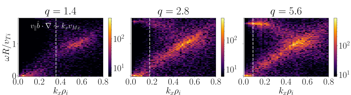
Figure 10: Zonal flow spectra $\absolutevalue{(v_{E}^{\mathrm{ZF}}R/v_{Ti}\rho_{i})_{k_{x},\omega}}$ in nonlinear gyrokinetic simulations of ITG turbulence for varying safety factor $q$. Only positive frequencies are shown here for clarity as the ZF amplitude at negative frequencies is very similar to that at positive frequencies, see e.g. Figure 1. The dashed line at $k_{x}\rho_{i}=1/2q$ is the wavenumber where the parallel streaming rate $v_{\parallel}\boldsymbol{\hat{b}}\cdot\nabla\sim v_{Ti}/qR$ and mode frequency $\omega\approx 2k_{x}\rho_{i}v_{Ti}/R$ are comparable.

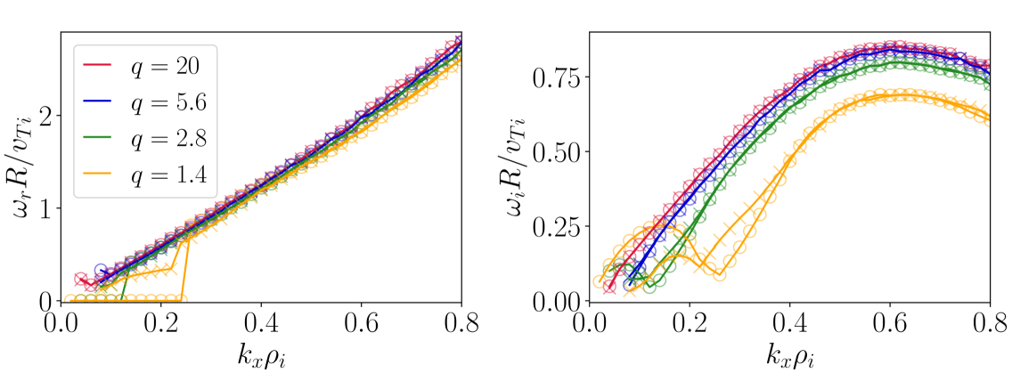
Figure 11: Secondary mode frequency (left) and growth rate (right) from gyrokinetic simulations of secondary modes for varying safety factor $q$ and phase-shift factors $\Theta=0$ (circles) and $\Theta=0.288572618$ (crosses). The primary distribution has the form (22) with $\eta_{\perp}^{P}=\eta_{\parallel}^{P}=3$, amplitude $\mathcal{A}^{P}=2$, and it varies along the magnetic field as $g_{i}^{P}\propto e^{-(\theta/\pi)^{2}}$.

As the wavenumber threshold is approached from above, the toroidal secondary modes become Landau damped, as shown in Figure 11. This damping by parallel streaming may further be interpreted as the short-circuiting of the regions below and above the midplane via parallel fluxes of particles and energy that reduce the up-down pressure asymmetry generating the TSM. Landau damping is also known to damp GAMs, with a typical scaling of the damping rate Im$(\omega_{\mathrm{GAM}})\propto-e^{-q^{2}}$ in tokamaks, such that GAMs are more often observed in the edge than in the core of tokamak devices. While the Landau damping of TSMs is expected to be stronger than that of GAMs due to the TSM’s smaller frequency (see e.g. Figure 1), the TSM drive by turbulence is also typically stronger. For this reason, the GAM amplitude is small in the turbulence simulations at low safety factor $q=1.4$ and $q=2.8$ (see Figure 11), while the TSM amplitude remains sizeable at short radial wavelengths $k_{x}\rho_{i}\sim 0.5$.

The choice of boundary conditions, e.g. the choice of $\Theta$ in (25), becomes important as parallel streaming becomes relevant to the mode dynamics. Indeed, Figure 11 shows that the choice of $\Theta$ affects the damping of toroidal secondary modes and, more importantly, $\Theta$ determines whether growing modes exist at long radial wavelengths. Effects of parallel streaming on the RDK secondary mode are to be expected for $k_{x}\tilde{v}_{g}^{P}\lesssim v_{\parallel}\boldsymbol{\hat{b}}\cdot\nabla$. Therefore, while we found in Section 3.4 that the RDK secondary mode mechanism is dominant at short wavelengths ($k_{x}\tilde{v}_{Mx}\gtrsim v_{\parallel}\boldsymbol{\hat{b}}\cdot\nabla$) only for large primary amplitudes $k_{x}\tilde{v}_{g}^{P}\gtrsim\omega_{\mathrm{GAM}}$, this requirement may be relaxed to $k_{x}\tilde{v}_{g}^{P}\gtrsim v_{\parallel}\boldsymbol{\hat{b}}\cdot\nabla$ at long wavelengths ($k_{x}\tilde{v}_{Mx}\lesssim v_{\parallel}\boldsymbol{\hat{b}}\cdot\nabla$). In the simulations with periodic boundary conditions $(\Theta=0)$, long-wavelength purely growing RDK secondary modes are observed also for weak primary drive $k_{x}\tilde{v}_{g}^{P}\lesssim v_{\parallel}\boldsymbol{\hat{b}}\cdot\nabla$, see Figure 11. In this case, the parallel streaming spreads the secondary mode along the field line, reducing the nonlinear interaction with the primary mode. Therefore, unlike for the TSM, the RDK secondary mode in this case has a reduced growth rate but it is not fully stabilised. For different boundary conditions at the ends of the flux tube, e.g. for different $\Theta$, the RDK secondary mode is affected differently, as may be seen in Figure 11.

Generally, one must be cautious to apply results of the secondary model in the regime of weak primary drive $k_{x}\tilde{v}_{g}^{P}\lesssim v_{\parallel}\boldsymbol{\hat{b}}\cdot\nabla$ and long radial wavelengths $k_{x}\tilde{v}_{Mx}\lesssim v_{\parallel}\boldsymbol{\hat{b}}\cdot\nabla$. Indeed, the separation of scales assumed in the secondary model can easily break, e.g. the binormal magnetic drift and the diamagnetic drift may become important, or the frozen streamer primary drive assumption may become unjustified because the primary drive will change significantly in a time comparable to the inverse of the secondary mode frequency. It may therefore be necessary to include more physics or to employ other models for the growth of zonal flows in this regime.

Finally, we note that the ISMs studied in this work are the secondary mode equivalents of the toroidal branch of the ITG. Introducing parallel streaming dynamics brings about the slab branch of the ITG (Cowley et al., 1991) and should therefore also give rise to a slab branch of the ISM. Such modes have been considered previously, see e.g. Drake et al. (1988); Cowley et al. (1991); Rath and Sridhar (1992); Ivanov et al. (2022), and will not be studied further here.

4 Summary and discussion

We have shown in this study how toroidicity affects the nonlinear physics of zonal flows. We refer back to Figure 2 for an overview of the modes discussed in this study and their respective regions of validity.

The secondary model was used to derive the dispersion relation (31), notably describing the toroidal secondary mode (TSM), a branch of growing and radially propagating zonal flows introduced in Nies et al. (2024). The theory also led to the dispersion relation (30) for ITG secondary modes (ISMs), secondary modes localised around particular points on the flux surface and driven unstable by the primary temperature gradient, see Section 3.2. The physical mechanism that drives the TSM, based on the Stringer-Winsor force and the generation of up-down pressure asymmetry through a combination of zonal flow shearing and advection by the radial magnetic drift, was studied in Section 3.3.

By considering the non-resonant limit of the secondary modes, we investigated in Section 3.4 the regions in parameter space where the RDK secondary modes, TSMs, and ISMs grow. The RDK secondary mode limit was found to require a large primary drive $k_{x}v_{Ex}^{P}\gg\omega_{\mathrm{GAM}}\sim v_{Ti}/R$, though this requirement might be relaxed at long wavelengths due to parallel streaming, as discussed in Section 3.5.2. The TSM was shown in Figure 8 to be driven unstable for sufficiently large primary temperature gradient drive, similar to the ISM, though the TSM is a global mode on the flux surface and is dominant over the ISM at sufficiently large primary drive (see (63) and surrounding discussion).

The effects of finite binormal wavenumbers and parallel streaming were considered in Section 3.5. Importantly, these effects were shown in Figures 9 and 11 to introduce a $k_{x}$-threshold for the TSM. In GK simulations of strongly driven tokamak ITG turbulence, the threshold is set by the parallel streaming to $k_{x}\rho_{i}\approx 1/2q$, as demonstrated by Figures 1 and 10.

Additional physical effects not considered in this work that might affect the TSM include background flow shear, non-adiabatic electron physics, collisions, and electromagnetic fluctuations. Future work could extend the secondary model of Section 3.1 to include these effects. Furthermore, the simulations presented in this study considered a circular cross-section tokamak for simplicity. Shaped tokamak and stellarator geometries might affect the toroidal secondary modes in interesting ways, e.g. tokamaks with a single X-point have an inherent up-down asymmetry that could interplay with the TSM mechanism.

The TSM is very prominent in gyrokinetic simulations of ITG turbulence (see Figures 1 and 10) and was shown in Nies et al. (2024) to contribute to turbulence saturation. The TSM could also potentially explain the avalanches widely reported in gyrokinetic simulations. Across our simulations (see Figures 1 and 10), the TSMs are observed predominantly at radial wavelengths $k_{x}\rho_{i}\approx 0.5$ and frequencies $\omega\approx v_{Ti}/R$, such that their associated propagation velocity is $v_{\mathrm{prop}}\approx 2v_{Ti}\rho_{i}/R$. A preliminary analysis suggests the TSM scale and propagation speed are consistent with the avalanches reported in McMillan et al. (2009); Idomura et al. (2009); Görler et al. (2010); Villard et al. (2014); Rath et al. (2016); Wang et al. (2017).

Moreover, zonal oscillations at $\omega\approx\omega_{\mathrm{GAM}}/2\approx v_{Ti}/R$, close to the dominant TSM frequency in turbulence simulations (see Figures 1 and 10), have been reported in tokamak I-mode experiments (Feng et al., 2019; McCarthy, 2022; Bielajew et al., 2022; Liu et al., 2023). The edge temperature ring oscillations observed in the EAST tokamak (Feng et al., 2019; Liu et al., 2023) could potentially be explained by the Stringer-Winsor force having to vanish, similar to the TSM (see also left column in Figure 6). One might thus speculate whether the TSM explains these low-frequency zonal modes. We note that it has been suggested that these oscillations are instead explained by Q-GAMs (Lee and Lee, 2024), which share some similarities with the TSM. Both the Q-GAM and the TSM are driven by the SW force mechanism, though the required up-down pressure asymmetry for the Q-GAM originates from background parallel fluxes, unlike the TSM for which it is generated by a combination of ZF shearing and radial magnetic drift advection (see Section 3.3 and Nies et al. (2024)).

Appendix A Strongly-driven secondary modes at long perpendicular wavelengths

In this appendix, we consider the growth of secondary modes in the limit of large primary drive and long perpendicular wavelengths. Unlike the theory presented in the main text and B, we do not assume the primary drive to be a streamer, i.e. $\partial_{x}g_{i}^{P}$ need not be zero. The primary drive is still assumed to be purely nonzonal, i.e. $\langle g_{i}^{P}\rangle_{y}=0$.

We consider two expansion parameters $\epsilon_{\mathrm{SD}}\ll 1$ and $\epsilon_{\mathrm{LW}}\ll 1$, with

$$v_{\parallel}\boldsymbol{\hat{b}}\cdot\nabla g_{i}^{S}\sim\mathop{}\!\boldsymbol{\tilde{v}}_{Mi}\cdot\nabla g_{i}^{S}\sim\langle\mathop{}\!\boldsymbol{v}_{E}^{S}\rangle_{\mathop{}\!\boldsymbol{R}_{i}}\cdot\nabla F_{Mi}\sim\epsilon_{\mathrm{SD}}\partial_{t}g_{i}^{S}\sim\epsilon_{\mathrm{SD}}\langle\mathop{}\!\boldsymbol{v}_{E}^{S}\rangle_{\mathop{}\!\boldsymbol{R}_{i}}\cdot\nabla g_{i}^{P}\sim\epsilon_{\mathrm{SD}}\langle\mathop{}\!\boldsymbol{v}_{E}^{P}\rangle_{\mathop{}\!\boldsymbol{R}_{i}}\cdot\nabla g_{i}^{S},$$ (64)

corresponding to a strong primary drive in the gyrokinetic equation for the secondary (11), and

$$\rho_{i}\nabla_{\perp}\ln g_{i}^{S}\sim\rho_{i}\nabla_{\perp}\ln g_{i}^{P}\sim\epsilon_{\mathrm{LW}},$$ (65)

corresponding to long perpendicular wavelengths. We note that $g_{i}^{S}/F_{Mi}\sim Z_{i}e\varphi^{S}/T_{i}$ is assumed throughout.

For long perpendicular wavelengths $\epsilon_{\mathrm{LW}}\ll 1$, gyro-averages may be approximated as

$$\langle f(\mathop{}\!\boldsymbol{r})\rangle_{\mathop{}\!\boldsymbol{R}_{i}}\approx\left(1+\frac{v_{\perp}^{2}}{4v_{Ti}^{2}}\rho_{i}^{2}\nabla_{\perp}^{2}\right)f(\mathop{}\!\boldsymbol{R}_{i}),\qquad\langle f(\mathop{}\!\boldsymbol{R}_{i})\rangle_{\mathop{}\!\boldsymbol{r}}\approx\left(1+\frac{v_{\perp}^{2}}{4v_{Ti}^{2}}\rho_{i}^{2}\nabla_{\perp}^{2}\right)f(\mathop{}\!\boldsymbol{r}).$$ (66)

The vorticity equation (9) may then be shown to simplify to

$$-\partial_{t}\left\langle\frac{\rho_{i}^{2}\absolutevalue{\nabla x}^{2}\partial_{x}^{2}\varphi^{S}}{2}\right\rangle_{\psi}= -\partial_{x}^{2}\left\langle\frac{\rho_{i}^{2}}{2}\left[\nabla x\cdot\nabla\varphi^{P}(v_{Ex}^{S}+v_{\mathrm{dia}}^{S})+\nabla x\cdot\nabla\varphi^{S}(v_{Ex}^{P}+v_{\mathrm{dia}}^{P})\right]\right\rangle_{\psi}$$

$$-\frac{T_{i}}{Z_{i}en_{i}}\left\langle\int\mathrm{d}^{3}v\,\tilde{v}_{Mx}\partial_{x}\left(g_{i}^{S}+\frac{Z_{i}e\varphi^{S}}{T_{i}}F_{Mi}\right)\right\rangle_{\psi},$$ (67)

with the primary $\mathop{}\!\boldsymbol{E}\times\mathop{}\!\boldsymbol{B}$ and diamagnetic velocities defined in (17) and (46), respectively. The definition of $v_{Ex}^{S}$ and $v_{\mathrm{dia}}^{S}$ is identical to that for the primary quantities, except for the replacement of the primary electrostatic potential and distribution function with the secondary ones. The three terms in (A) correspond to the ZF inertia, the nonlinear Reynolds and diamagnetic stresses, and the Stringer-Winsor (SW) force (see also discussion around (9)).

It is convenient to define the deviation of the electrostatic potential from its flux-surface averaged value,

$$\delta\varphi\equiv\varphi-\langle\varphi\rangle_{\psi},$$ (68)

with $\langle\delta\varphi\rangle_{\psi}=0$ by definition. The smallness of $\epsilon_{\mathrm{SD}}$ and $\epsilon_{\mathrm{LW}}$ may be used to expand $g_{i}^{S}$ and $\delta\varphi^{S}$ as

$$g_{i}^{S}=g_{i0}^{S}+g_{i1}^{S}+\mathcal{O}(\epsilon_{\mathrm{SD}}^{2}g_{i}^{S})+\mathcal{O}(\epsilon_{\mathrm{LW}}^{2}g_{i}^{S}),\qquad\delta\varphi^{S}=\delta\varphi_{0}^{S}+\delta\varphi_{1}^{S}+\mathcal{O}(\epsilon_{\mathrm{SD}}^{2}\delta\varphi^{S})+\mathcal{O}(\epsilon_{\mathrm{LW}}^{2}\delta\varphi^{S}),$$ (69)

with $g_{i1}^{S}\sim\epsilon_{\mathrm{SD}}g_{i}^{S}$ and $\delta\varphi_{1}^{S}\sim\epsilon_{\mathrm{SD}}\delta\varphi^{S}$. There are no contributions to $\mathcal{O}(\epsilon_{\mathrm{LW}}g_{i}^{S})$ and $\mathcal{O}(\epsilon_{\mathrm{LW}}\delta\varphi^{S})$ as demonstrated by the fact that (66) only contains corrections quadratic in $\epsilon_{\mathrm{LW}}$. Various moments of $g_{i}^{S}$ used below will follow the same notation for the expansion as $\delta\varphi^{S}$, e.g. $P^{S}=P_{0}^{S}+P_{1}^{S}+...$ for the pressure-like quantity defined in (37).

To leading order, the GK equation (11) gives

$$\partial_{t}g_{i0}^{S}=-\{\varphi^{P},g_{i0}^{S}\}-\{\langle\varphi^{S}\rangle_{\psi}+\delta\varphi_{0}^{S},g_{i}^{P}\},$$ (70)

where we have written the advection by the $\mathop{}\!\boldsymbol{E}\times\mathop{}\!\boldsymbol{B}$ flow using the Poisson bracket

$$\{f,g\}=\frac{\boldsymbol{\hat{b}}\cdot\nabla x\times\nabla y}{B}\left(\partial_{x}f\partial_{y}g-\partial_{y}f\partial_{x}g\right)$$ (71)

such that $\mathop{}\!\boldsymbol{v}_{E}\cdot\nabla g_{i}=\{\varphi,g_{i}\}$. Again to leading order, taking a time derivative of the quasineutrality equation (12) and inserting (70) leads to

$$\partial_{t}\delta\varphi_{0}^{S}=-\{\langle\varphi^{S}\rangle_{\psi},\varphi^{P}\}.$$ (72)

The nonzonal secondary potential thus evolves due to the zonal flow advecting the primary potential. Differentiating (70) with respect to $t$ leads to

$$0=\partial_{t}\left(\partial_{t}g_{i0}^{S}+\{\langle\varphi^{S}\rangle_{\psi},g_{i}^{P}\}\right)+\{\varphi^{P},\partial_{t}g_{i0}^{S}+\{\langle\varphi^{S}\rangle_{\psi},g_{i}^{P}\}\}-\{\langle\varphi^{S}\rangle_{\psi},\{\varphi^{P},g_{i}^{P}\}\},$$ (73)

where we used the Leibniz identity for Poisson brackets

$$\{f,\{g,h\}\}+\{g,\{h,f\}\}+\{h,\{f,g\}\}=0.$$ (74)

We assume the primary drive to not be self-interacting, i.e. $\{\varphi^{P},g_{i}^{P}\}=0$, such that the last term in (73) vanishes. A nonlinearly self-interacting primary drive would lead to a ‘forced’ growth of the ZF, different from the modulational instability mechanism studied in this work. The self-interaction can be important in the case of ZFs driven by Alfvén primary modes due to their global character, see e.g. Qiu et al. (2016). In the case of ZF drive by turbulent fluctuations, the self-interaction becomes important when the primary modes are elongated enough along the magnetic field to ‘bite their own tail’ (C. J. et al., 2020). We do not consider such cases here. Then, the quantity

$$G^{S}=\partial_{t}g_{i0}^{S}+\{\langle\varphi^{S}\rangle_{\psi},g_{i}^{P}\}$$ (75)

is simply advected by the primary $\mathop{}\!\boldsymbol{E}\times\mathop{}\!\boldsymbol{B}$ flow,

$$\partial_{t}G^{S}+\{\varphi^{P},G^{S}\}=0.$$ (76)

This advection does not lead to exponential growth, so we limit ourselves to the case $G^{S}=0$. We therefore obtain

$$\partial_{t}g_{i0}^{S}=-\{\langle\varphi^{S}\rangle_{\psi},g_{i}^{P}\}.$$ (77)

To leading order, the secondary distribution thus results purely from the zonal flow advecting the primary distribution function and is therefore nonzonal, $\langle g_{i0}^{S}\rangle_{\psi}=0$. This is not in contradiction with the zonal flow being finite at lowest order because of the factor $(1-\Gamma_{0i})\sim\epsilon_{\mathrm{LW}}^{2}$ in the quasineutrality equation (8), such that the zonal flow is contained in the higher order contribution $\mathcal{O}(\epsilon_{\mathrm{LW}}^{2})$ to $g_{i}^{S}$.

The leading order expressions (72) and (77) are sufficient to derive a dispersion relation for the RDK secondary modes (Rogers et al., 2000). Using

$$-\partial_{t}\left(\nabla x\cdot\nabla\varphi^{P}(v_{Ex,0}^{S}+v_{\mathrm{dia,0}}^{S})+\nabla x\cdot\nabla\delta\varphi_{0}^{S}(v_{Ex}^{P}+v_{\mathrm{dia}}^{P})\right)$$

$$=\nabla x\cdot\nabla\varphi^{P}\{\langle\varphi^{S}\rangle_{\psi},\left(v_{Ex}^{P}+v_{\mathrm{dia}}^{P}\right)\}+\nabla x\cdot\nabla\{\langle\varphi^{S}\rangle_{\psi},\varphi^{P}\}\left(v_{Ex}^{P}+v_{\mathrm{dia}}^{P}\right)$$

$$=\absolutevalue{\nabla x}^{2}\partial_{x}^{2}\langle\varphi^{S}\rangle_{\psi}v_{Ex}^{P}\left(v_{Ex}^{P}+v_{\mathrm{dia}}^{P}\right)+\left\{\langle\varphi^{S}\rangle_{\psi},\nabla x\cdot\nabla\varphi^{P}\left(v_{Ex}^{P}+v_{\mathrm{dia}}^{P}\right)\right\},$$ (78)

the time derivative of the vorticity equation (A) simplifies to

$$-\left\langle\frac{\rho_{i}^{2}\absolutevalue{\nabla x}^{2}}{2}\right\rangle_{\psi}\partial_{t}^{2}\partial_{x}^{2}\langle\varphi^{S}\rangle_{\psi}= \partial_{x}^{2}\left(\partial_{x}^{2}\langle\varphi^{S}\rangle_{\psi}\left\langle\frac{\rho_{i}^{2}\absolutevalue{\nabla x}^{2}}{2}v_{Ex}^{P}\left(v_{Ex}^{P}+v_{\mathrm{dia}}^{P}\right)\right\rangle_{\psi}\right)$$

$$-\left\langle v_{Mx}\partial_{x}\partial_{t}\left(\frac{P_{1}^{S}}{Z_{i}en_{i}}+\delta\varphi_{1}^{S}\right)\right\rangle_{\psi}.$$ (79)

Here, we have used the definition of the pressure-like quantity $P$ in (37) and $\langle\{\langle\varphi^{S}\rangle_{\psi},f\}\rangle_{\psi}=0$. This latter identity, combined with $\langle v_{Mx}\rangle_{\psi}=0$, causes the SW force contribution to vanish at $\mathcal{O}(\epsilon_{\mathrm{SD}})$, and the higher order contributions $P_{1}^{S}$ and $\delta\varphi_{1}^{S}$ must therefore be derived to evaluate it.

In the limit $\epsilon_{\mathrm{SD}}\ll\epsilon_{\mathrm{LW}}$, the SW force contribution may be ignored entirely ($P_{1}^{S},\delta\varphi_{1}^{S}\rightarrow 0$) and (A) describes the RDK secondary mode (Rogers et al., 2000). The equation thus obtained is somewhat more general than previous work which assumed the primary drive to have large radial scales compared to the secondary mode, by either assuming the primary mode to be a streamer ($\partial_{x}g_{i}^{P}=0$) (Rogers et al., 2000; Plunk, 2007) or by employing a WKB approximation (Plunk and Navarro, 2017). It is worth noting that the equations (72) and (77) justify the use of 4MT (four mode truncation) models to describe the RDK secondary mode: for a primary drive described by the Fourier mode $(k_{x}=0,k_{y}=k_{y}^{P})$, the secondary mode will be fully described by a zonal mode $(k_{x}=k_{x}^{S},k_{y}=0)$ and the sidebands $(k_{x}=k_{x}^{S},k_{y}=\pm k_{y}^{P})$. This is not the case for electron-scale secondary modes (Plunk, 2007) or for secondary modes with finite radial magnetic drift (27). In these cases, the secondary distribution and potential generally consist of many Fourier modes in $k_{y}$ even when the primary drive is described by a single Fourier mode. For an $x$-independent primary drive, Fourier-Laplace transforming (A) in $x$ and $t$ leads to the RDK secondary mode dispersion relation (51). We note that a dispersion relation for RDK secondary modes for arbitrary radial wavelengths of the secondary mode ($\epsilon_{\mathrm{LW}}\sim 1$) may be derived assuming a streamer primary mode $(\partial_{x}g_{i}^{P}=0)$, as shown in B.

We now consider $\epsilon_{\mathrm{SD}}\sim\epsilon_{\mathrm{LW}}$, in which case we must compute the corrections $g_{i1}^{S}$ and $\delta\varphi_{1}^{S}$ to the secondary distribution and electrostatic potential so as to be able to evaluate the SW force contribution to the vorticity equation. First, we define various velocity-space moments that will prove useful, i.e. the parallel flow

$$u_{\parallel}=\frac{1}{n_{i}}\int\mathrm{d}^{3}v\,v_{\parallel}g_{i},$$ (80)

the parallel flux of parallel energy

$$q_{\parallel}=\int\mathrm{d}^{3}v\,v_{\parallel}\frac{m_{i}v_{\parallel}^{2}}{2}g_{i},$$ (81)

the parallel flux of perpendicular energy

$$q_{\perp}=\int\mathrm{d}^{3}v\,v_{\parallel}\frac{m_{i}v_{\perp}^{2}}{2}g_{i},$$ (82)

and finally the fourth-order moment (with units of pressure)

$$\chi=T_{i}\int\mathrm{d}^{3}v\,\left(\frac{v_{\parallel}^{2}+v_{\perp}^{2}/2}{v_{Ti}^{2}}\right)^{2}g_{i}.$$ (83)

The GK equation (11) at $\mathcal{O}(\epsilon_{\mathrm{SD}}\partial_{t}g_{i}^{S})$ is given by

$$\partial_{t}g_{i1}^{S}+\{\varphi^{P},g_{i1}^{S}\}+\{\delta\varphi_{1}^{S},g_{i}^{P}\}=-\left(v_{\parallel}\boldsymbol{\hat{b}}+\tilde{\mathop{}\!\boldsymbol{v}}_{M}\right)\cdot\nabla\left(g_{i0}^{S}+\frac{Z_{i}e(\langle\varphi^{S}\rangle_{\psi}+\delta\varphi_{0}^{S})}{T_{i}}F_{Mi}\right)-\{\delta\varphi_{0}^{S},F_{Mi}\}.$$ (84)

To evaluate the SW force contribution, we must evaluate the time derivatives of $P_{1}^{S}$ and $\delta\varphi_{1}^{S}$. The latter is obtained by considering the time derivative of the quasineutrality equation (12) to $\mathcal{O}(\epsilon_{\mathrm{SD}}\varphi^{S})$,

$$\tau\partial_{t}\delta\varphi_{1}^{S}=\frac{T_{i}}{Z_{i}en_{i}}\int\mathrm{d}^{3}v\,\partial_{t}g_{i1}^{S}.$$ (85)

Using (84), we derive

$$\tau\frac{Z_{i}e}{T_{i}}\partial_{t}\delta\varphi_{1}^{S}=-\mathop{}\!\boldsymbol{B}\cdot\nabla\left(\frac{u_{\parallel,0}^{S}}{B}\right)-\mathop{}\!\boldsymbol{v}_{M}\cdot\nabla\left(\frac{P_{0}^{S}}{n_{i}T_{i}}+\frac{Z_{i}e(\langle\varphi^{S}\rangle_{\psi}+\delta\varphi_{0}^{S})}{T_{i}}\right)-v_{Ex,0}^{S}\partial_{x}\ln n_{i}.$$ (86)

Here, we have used

$$\mathrm{d}^{3}v=\frac{2\pi B}{m_{i}^{2}\absolutevalue{v_{\parallel}}}\sum_{\mathrm{sgn}(v_{\parallel})}\mathrm{d}E_{i}\mathrm{d}\mu_{i},$$ (87)

with the ion energy $E_{i}=m_{i}v^{2}/2$ and magnetic moment $\mu_{i}=m_{i}v_{\perp}^{2}/2B$, which are held constant as the spatial derivatives are evaluated. Furthermore, we assumed for simplicity that the pressure gradient contribution to the magnetic drift in (2) is negligible, which is satisfied e.g. at low plasma beta, $\beta\equiv 2\mu_{0}p/B^{2}\ll 1$. The magnetic drift velocity may then be written as

$$\tilde{\mathop{}\!\boldsymbol{v}}_{M}=\mathop{}\!\boldsymbol{v}_{M}\frac{v_{\parallel}^{2}+v_{\perp}^{2}/2}{v_{Ti}^{2}},$$ (88)

similar to the expression for the radial component of the magnetic drift (10). If needed, the pressure gradient contribution to the curvature drift could be kept, at the price of another moment of the distribution function to carry through in the derivation. We note that (86) satisfies the consistency condition $\langle\delta\varphi_{1}^{S}\rangle_{\psi}=0$, as $\langle v_{Mx}\rangle_{\psi}=0$ and the leading order distribution function $g_{i0}^{S}$ is nonzonal (see (77)).

The time derivative of the pressure moment $P_{1}^{S}$ is derived by evaluating the appropriate moment of (84),

$$\partial_{t}P_{1}^{S}+ \{\varphi^{P},P_{1}^{S}\}+\{\delta\varphi_{1}^{S},P^{P}\}=-\mathop{}\!\boldsymbol{B}\cdot\nabla\left(\frac{q_{\parallel,0}^{S}}{B}\right)-\frac{\boldsymbol{\hat{b}}\cdot\nabla q_{\perp,0}^{S}}{2}$$

$$-\mathop{}\!\boldsymbol{v}_{M}\cdot\nabla\left(\chi_{0}^{S}+\frac{7}{4}Z_{i}en_{i}(\langle\varphi^{S}\rangle_{\psi}+\delta\varphi_{0}^{S})\right)-v_{Ex,0}^{S}\partial_{x}(n_{i}T_{i}).$$ (89)

The SW force contribution due to $\delta\varphi_{1}^{S}$ in (A) is derived from (86) to have the simple form

$$\left\langle v_{Mx}\partial_{x}\partial_{t}\delta\varphi_{1}^{S}\right\rangle_{\psi}=-\frac{1}{\tau}\left\langle v_{Mx}^{2}\right\rangle_{\psi}\partial_{x}^{2}\langle\varphi^{S}\rangle_{\psi}.$$ (90)

Note that many terms in (86) have not contributed to (90) because the average over $y$ of $g_{i0}^{S}$ vanishes due to (77).

Evaluating the contribution of $P_{1}^{S}$ to the SW force is more involved due to the presence of the primary $\mathop{}\!\boldsymbol{E}\times\mathop{}\!\boldsymbol{B}$-advection term in (89). One may simply consider the closed system of equations (72), (77), (A), (86), and (89) to describe the evolution of strongly driven secondary modes at long perpendicular wavelengths. This system of equations describes how the leading order secondary distribution function $g_{i0}^{S}$ and nonzonal potential fluctuation $\delta\varphi_{0}^{S}$, which due to (77) and (72) result from the zonal flow shearing of the primary distribution and potential, source higher order pressure and potential fluctuations $P_{1}^{S}$ and $\delta\varphi_{1}^{S}$ through parallel streaming, magnetic drifts, and the $\mathop{}\!\boldsymbol{E}\times\mathop{}\!\boldsymbol{B}$-mixing of the background Maxwellian. Then, $P_{1}^{S}$ and $\delta\varphi_{1}^{S}$ feed back on the zonal flow generation through the SW force, with the contribution from $\delta\varphi_{1}^{S}$ evaluated in (90).

To derive a more explicit dispersion relation, we Laplace-transform the secondary distribution in time and consider exponentially growing solutions $\varphi^{S}=\hat{\varphi}^{S}e^{-i\omega t}$ (similar notation will be used for $g_{i}^{S}$ and its velocity-space moments) with Im$(\omega)>0$. Furthermore we define the differential operator $\omega_{E}^{P}$ such that

$$i\omega_{E}^{P}f=\{\varphi^{P},f\},$$ (91)

which represents the advection by the primary $\mathop{}\!\boldsymbol{E}\times\mathop{}\!\boldsymbol{B}$ flow. The leading order expressions (72) and (77) may now be expressed as

$$i\omega\delta\hat{\varphi}_{0}^{S}=\{\langle\hat{\varphi}^{S}\rangle_{\psi},\varphi^{P}\},\qquad i\omega\hat{g}_{i0}^{S}=\{\langle\hat{\varphi}^{S}\rangle_{\psi},g_{i}^{P}\}.$$ (92)

Furthermore, we obtain

$$-i\omega\, \tau\frac{Z_{i}e\delta\hat{\varphi}_{1}^{S}}{T_{i}}=-v_{Mx}\partial_{x}\left(\frac{Z_{i}e\langle\hat{\varphi}^{S}\rangle_{\psi}}{T_{i}}\right)-\frac{1}{i\omega}\left\{v_{Mx}\partial_{x}\langle\hat{\varphi}^{S}\rangle_{\psi},\frac{P^{P}}{n_{i}T_{i}}+\frac{Z_{i}e\varphi^{P}}{T_{i}}\right\}$$

$$- \frac{1}{i\omega}\left\{\langle\hat{\varphi}^{S}\rangle_{\psi},\mathop{}\!\boldsymbol{B}\cdot\nabla\left(\frac{u_{\parallel}^{P}}{B}\right)+\mathop{}\!\boldsymbol{v}_{M}\cdot\nabla\left(\frac{P^{P}}{n_{i}T_{i}}+\frac{Z_{i}e\varphi^{P}}{T_{i}}\right)+v_{Ex}^{P}\partial_{x}\ln n_{i}\right\}$$ (93)

from (72), (77), and (86), as well as

$$-i (\omega-\omega_{E}^{P})\hat{P}_{1}^{S}=-\{\delta\varphi_{1}^{S},P^{P}\}-\frac{7}{4}Z_{i}en_{i}v_{Mx}\partial_{x}\langle\hat{\varphi}^{S}\rangle_{\psi}-\frac{1}{i\omega}\left\{v_{Mx}\partial_{x}\langle\hat{\varphi}^{S}\rangle_{\psi},\chi^{P}+\frac{7}{4}Z_{i}en_{i}\varphi^{P}\right\}$$

$$- \frac{1}{i\omega}\left\{\langle\hat{\varphi}^{S}\rangle_{\psi},\mathop{}\!\boldsymbol{B}\cdot\nabla\left(\frac{q_{\parallel}^{P}}{B}\right)+\frac{\boldsymbol{\hat{b}}\cdot\nabla q_{\perp}^{P}}{2}+\mathop{}\!\boldsymbol{v}_{M}\cdot\nabla\left(\chi^{P}+\frac{7}{4}Z_{i}en_{i}\varphi^{P}\right)+v_{Ex}^{P}\partial_{x}(n_{i}T_{i})\right\}$$ (94)

from (77), (89), and (91). The latter expression may also be written as

$$-i \omega\hat{P}_{1}^{S}=-\frac{7}{4}Z_{i}en_{i}v_{Mx}\partial_{x}\langle\hat{\varphi}^{S}\rangle_{\psi}+i(\omega-\omega_{E}^{P})^{-1}\Bigg{[}i\omega\{\delta\hat{\varphi}_{1}^{S},P^{P}\}+\left\{v_{Mx}\partial_{x}\langle\hat{\varphi}^{S}\rangle_{\psi},\chi^{P}\right\}$$

$$+\left\{\langle\hat{\varphi}^{S}\rangle_{\psi},\mathop{}\!\boldsymbol{B}\cdot\nabla\left(\frac{q_{\parallel}^{P}}{B}\right)+\frac{\boldsymbol{\hat{b}}\cdot\nabla q_{\perp}^{P}}{2}+\mathop{}\!\boldsymbol{v}_{M}\cdot\nabla\left(\chi^{P}+\frac{7}{4}Z_{i}en_{i}\varphi^{P}\right)+v_{Ex}^{P}\partial_{x}(n_{i}T_{i})\right\}\Bigg{]}.$$ (95)

The expressions (93) and (95) can now be inserted into (A) to derive a dispersion relation for secondary modes. We do not write this expression out due to its unwieldiness. Note that solving this dispersion relation would require the evaluation of the operator $(\omega-\omega_{E}^{P})^{-1}$.

For simplicity, we now consider an up-down symmetric tokamak and assume the even moments of $g_{i}^{P}$ in $v_{\parallel}$ (e.g. the gyrocentre density and pressure) to be symmetric in $\theta$ while the odd moments of $g_{i}^{P}$ in $v_{\parallel}$ (e.g. the parallel flow and parallel fluxes) are antisymmetric in $\theta$. For a primary drive representing a linearly unstable mode, these assumptions are justified based on the symmetry of the linear GK equation (Peeters et al., 2005). Then, $\varphi^{P},P^{P},\chi^{P},\boldsymbol{\hat{b}}\cdot\nabla u_{\parallel}^{P},\boldsymbol{\hat{b}}\cdot\nabla q_{\parallel}^{P},\boldsymbol{\hat{b}}\cdot\nabla q_{\perp}^{P}$ are all taken to be up-down symmetric. Furthermore, the binormal component of the magnetic drift is also up-down symmetric. For example, for a large aspect ratio tokamak with circular flux surfaces, the radial and binormal magnetic drift components vary along the field line as $\mathop{}\!\boldsymbol{v}_{M}\cdot\nabla x\propto\sin\theta$ and $\mathop{}\!\boldsymbol{v}_{M}\cdot\nabla y\propto\cos\theta+\hat{s}\theta\sin\theta$, respectively. In that case, the only non-vanishing contributions to the SW force from $P_{1}^{S}$ and $\delta\varphi_{1}^{S}$ stem from the radial magnetic drift contributions in (93) and (95). Therefore, for an up-down symmetric tokamak with up-down symmetric primary drive, equation (A) gives

$$\omega^{2}\left\langle\frac{\rho_{i}^{2}\absolutevalue{\nabla x}^{2}}{2}\right\rangle_{\psi}\partial_{x}^{2}\langle\hat{\varphi}^{S}\rangle_{\psi} =\partial_{x}^{2}\left(\partial_{x}^{2}\langle\hat{\varphi}^{S}\rangle_{\psi}\left\langle\frac{\rho_{i}^{2}\absolutevalue{\nabla x}^{2}}{2}v_{Ex}^{P}\left(v_{Ex}^{P}+v_{\mathrm{dia}}^{P}\right)\right\rangle_{\psi}\right)+\partial_{x}^{2}\langle\hat{\varphi}^{S}\rangle_{\psi}\langle v_{Mx}^{2}\rangle_{\psi}\left(\frac{7}{4}+\frac{1}{\tau}\right)$$

$$-\partial_{x}\Bigg{\langle}v_{Mx}i(\omega-\omega_{E}^{P})^{-1}\bigg{[} \frac{1}{\tau}\left\{v_{Mx}\partial_{x}\langle\hat{\varphi}^{S}\rangle_{\psi}+\frac{1}{i\omega}v_{Mx}\partial_{x}\left\{\langle\hat{\varphi}^{S}\rangle_{\psi},\frac{P^{P}}{Z_{i}en_{i}}+\varphi^{P}\right\},\frac{P^{P}}{Z_{i}en_{i}}\right\}$$

$$+v_{Mx}\partial_{x}\left\{\langle\hat{\varphi}^{S}\rangle_{\psi},\frac{\chi^{P}}{Z_{i}en_{i}}\right\}+\frac{7}{4}\left\{\langle\hat{\varphi}^{S}\rangle_{\psi},v_{Mx}\partial_{x}\varphi^{P}\right\}\bigg{]}\Bigg{\rangle}_{\psi}.$$ (96)

The theory in Section 3 assumes a streamer primary ($\partial_{x}g_{i}^{P}=0$), in which case the secondary mode may be Fourier expanded in $x$. The frequency of the secondary mode with wavenumber $k_{x}$ may then be derived from the dispersion relation (96) using the fact that the operator (91) simplifies to

$$\omega_{E}^{P}\,e^{ik_{x}x}=k_{x}v_{Ex}^{P}e^{ik_{x}x}.$$ (97)

The resulting dispersion relation is equation (49) in the main text and is discussed there in more detail.

Appendix B Rogers-Dorland-Kotschenreuther (RDK) secondary mode for arbitrary radial wavelengths

In A and Section 3.4, we discussed the RDK secondary mode in the limit of long perpendicular wavelengths. Here, we discuss the RDK secondary mode for arbitrary radial wavelengths. To this end, we assume a frozen streamer primary, like in the theory of the generalised secondary mode of Section 3.1, and we consider the limit of vanishing linear terms (magnetic drifts, parallel streaming, and diamagnetic drift) in the GK equation. A dispersion relation may therefore be derived from (31) with $\mathcal{N}$ evaluated in the limit of $\tilde{v}_{Mx}\rightarrow 0$. If we further assume the primary drive to be given by the bi-Maxwellian (22), equation (29) for $\mathcal{N}$ simplifies to

$$\mathcal{N}=-\frac{\tau k_{x}v_{Ex}^{P}}{\omega-k_{x}v_{Ex}^{P}}\left(\Gamma_{0i}(b_{i})+b_{i}\Gamma_{0i}^{\prime}(b_{i})\eta_{\perp}^{P}\right),$$ (98)

with $\Gamma_{0i}^{\prime}(b_{i})=\mathrm{d}\Gamma_{0i}(b_{i})/\mathrm{d}b_{i}$. The dispersion relation (31) becomes

$$0=1-\tau\left\langle\frac{\omega-k_{x}v_{Ex}^{P}}{\omega f_{\omega}-k_{x}v_{Ex}^{P}f_{E}}\right\rangle_{\psi},$$ (99)

which may be shown to be equivalent to equation (4) in Rogers et al. (2000). Here, we defined

$$f_{\omega}\equiv 1-\Gamma_{0i}+\tau,\qquad f_{E}\equiv(1-\Gamma_{0i})(1+\tau)-\tau\eta_{\perp}^{P}b_{i}\Gamma_{0i}^{\prime}.$$ (100)

We consider a primary drive sinusoidally varying in $y$ and constant along the magnetic field, $v_{Ex}^{P}=v_{Ex}^{P0}\sin(k_{y}^{P}y)$, and $\eta_{\perp}^{P}$ is taken to be constant. For simplicity, we further assume that the variation of $b_{i}$ along the magnetic field is negligible, as is appropriate for e.g. a large aspect ratio tokamak with circular flux surfaces. The flux-surface average in (99) then requires evaluating the integral

$$\frac{1}{2\pi}\int_{0}^{2\pi}\frac{\mathrm{d}\phi}{1-A\sin\phi}=\frac{1}{\sqrt{1-A^{2}}},$$ (101)

which may be obtained e.g. by changing variables to $z=e^{i\phi}$ and using the method of residues. Here, the square root is evaluated with the branch cut along negative reals such that Re$\sqrt{x}\geq 0$.

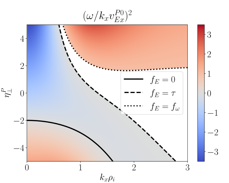
Figure 12: Rogers-Dorland-Kotschenreuther (RDK) secondary mode frequency from (106) for $b_{i}=k_{x}^{2}\rho_{i}^{2}/2$. The primary drive is given by (22), with $v_{Ex}^{P}=v_{Ex}^{P0}\sin(k_{y}^{P}y)$ and no variation along the magnetic field. There are no modes in the blank region ($\tau\leq f_{E}\leq f_{\omega}$), see (103). Purely growing RDK secondary modes ($\omega^{2}<0$) are found for $0<f_{E}<\tau$, see (105).

The dispersion relation (99) then simplifies to

$$0=1-\frac{\tau}{f_{E}}-\tau\left(\frac{1}{f_{\omega}}-\frac{1}{f_{E}}\right)\Bigg{/}\sqrt{1-\left(\frac{k_{x}v_{Ex}^{P0}f_{E}}{\omega f_{\omega}}\right)^{2}},$$ (102)

As the real part of the square root must be positive, a necessary condition for the existence of solutions to (102) is

$$\frac{f_{E}-f_{\omega}}{f_{E}-\tau}\geq 0.$$ (103)

When this condition is satisfied, rearranging and squaring (102) leads to the secondary mode frequency

$$\left(\frac{\omega}{k_{x}v_{Ex}^{P0}}\right)^{2}=\frac{(f_{E}-\tau)^{2}}{f_{\omega}-\tau}\frac{f_{E}}{f_{E}(f_{\omega}+\tau)-2\tau f_{\omega}}.$$ (104)

Noting that $f_{\omega}-\tau>0$ by (100), the mode is unstable when the second fraction in (104) is negative, i.e. $0<f_{E}<2\tau f_{\omega}/(\tau+f_{\omega})$. As the condition for mode existence (103) sets a stricter upper bound on $f_{E}$, the condition for the existence of unstable RDK secondary modes may be succinctly written as

$$0<f_{E}\leq\tau.$$ (105)

Using (100), the secondary mode frequency (104) may also be written as

$$\left(\frac{\omega}{k_{x}v_{Ex}^{P0}}\right)^{2}=\frac{\left(1-\Gamma_{0i}-\tau\Gamma_{0i}-\tau\eta_{\perp}^{P}b_{i}\Gamma_{0i}^{\prime}\right)^{2}}{1-\Gamma_{0i}}\frac{(1+\tau)(1-\Gamma_{0i})-\tau\eta_{\perp}^{P}b_{i}\Gamma_{0i}^{\prime}}{(1-\Gamma_{0i})^{2}(1+\tau)-2\tau^{2}\Gamma_{0i}-\tau\eta_{\perp}^{P}b_{i}\Gamma_{0i}^{\prime}\left(1-\Gamma_{0i}+2\tau\right)}.$$ (106)

which recovers equation (5) of Rogers et al. (2000) in the limit $\eta_{\perp}^{P}=0$. Condition (105) for instability may be written as

$$0<(1-\Gamma_{0i})(1+\tau)-\tau\eta_{\perp}^{P}b_{i}\Gamma_{0i}^{\prime}\leq\tau.$$ (107)

For small $b_{i}\ll 1$, the instability criterion simplifies to $\eta_{\perp}^{P}>-(1+\tau^{-1})$, as expected from the RDK dispersion relation for long perpendicular wavelengths (51). For large $b_{i}\gg 1$, for which $\Gamma_{0i}\approx(2\pi b_{i})^{-1/2}$, the second inequality in (107) is satisfied only for large negative $\eta_{\perp}^{P}$ values. Generally (for $\eta_{\perp}^{P}\sim 1$), there will therefore be no unstable RDK secondary mode for large $b_{i}\gg 1$, as shown in Figure 12.

References

- Barnes et al. [2011] M. Barnes, F. I. Parra, and A. A. Schekochihin. Critically Balanced Ion Temperature Gradient Turbulence in Fusion Plasmas. Physical Review Letters, 107(11):115003, September 2011. ISSN 0031-9007, 1079-7114. doi: 10.1103/PhysRevLett.107.115003. URL https://link.aps.org/doi/10.1103/PhysRevLett.107.115003.
- Barnes et al. [2019] M. Barnes, F.I. Parra, and M. Landreman. stella: An operator-split, implicit–explicit deltaf-gyrokinetic code for general magnetic field configurations. Journal of Computational Physics, 391:365–380, August 2019. ISSN 00219991. doi: 10.1016/j.jcp.2019.01.025. URL https://linkinghub.elsevier.com/retrieve/pii/S002199911930066X.
- Beer et al. [1995] M. A. Beer, S. C. Cowley, and G. W. Hammett. Field‐aligned coordinates for nonlinear simulations of tokamak turbulence. Physics of Plasmas, 2(7):2687–2700, August 1995. ISSN 1070-664X, 1089-7674. doi: 10.1063/1.871232. URL http://aip.scitation.org/doi/10.1063/1.871232.
- Bielajew et al. [2022] R. Bielajew, G. D. Conway, M. Griener, T. Happel, K. Höfler, N. T. Howard, A. E. Hubbard, W. McCarthy, P. A. Molina Cabrera, T. Nishizawa, P. Rodriguez-Fernandez, D. Silvagni, B. Vanovac, D. Wendler, C. Yoo, A. E. White, and ASDEX Upgrade Team. Edge turbulence measurements in L-mode and I-mode at ASDEX Upgrade. Physics of Plasmas, 29(5):052504, May 2022. ISSN 1070-664X, 1089-7674. doi: 10.1063/5.0088062. URL https://pubs.aip.org/pop/article/29/5/052504/2847917/Edge-turbulence-measurements-in-L-mode-and-I-mode.
- Biglari et al. [1989] H. Biglari, P. H. Diamond, and M. N. Rosenbluth. Toroidal ion‐pressure‐gradient‐driven drift instabilities and transport revisited. Physics of Fluids B: Plasma Physics, 1(1):109–118, January 1989. ISSN 0899-8221. doi: 10.1063/1.859206. URL http://aip.scitation.org/doi/10.1063/1.859206.
- C. J. et al. [2020] A. C. J., S. Brunner, B. McMillan, J. Ball, J. Dominski, and G. Merlo. How eigenmode self-interaction affects zonal flows and convergence of tokamak core turbulence with toroidal system size. Journal of Plasma Physics, 86(5):905860504, October 2020. ISSN 0022-3778, 1469-7807. doi: 10.1017/S0022377820000999. URL https://www.cambridge.org/core/product/identifier/S0022377820000999/type/journal_article.
- Catto [1978] P. J. Catto. Linearized gyro-kinetics. Plasma Physics, 20(7):719–722, July 1978. ISSN 0032-1028. doi: 10.1088/0032-1028/20/7/011. URL https://iopscience.iop.org/article/10.1088/0032-1028/20/7/011.
- Chen et al. [2000] L. Chen, Z. Lin, and R. White. Excitation of zonal flow by drift waves in toroidal plasmas. Physics of Plasmas, 7(8):3129–3132, August 2000. ISSN 1070-664X, 1089-7674. doi: 10.1063/1.874222. URL http://aip.scitation.org/doi/10.1063/1.874222.
- Conway et al. [2021] G. D. Conway, A. I. Smolyakov, and T. Ido. Geodesic acoustic modes in magnetic confinement devices. Nuclear Fusion, 62(1):013001, December 2021. ISSN 0029-5515. doi: 10.1088/1741-4326/ac0dd1. URL https://doi.org/10.1088/1741-4326/ac0dd1. Publisher: IOP Publishing.
- Coppi et al. [1967] B. Coppi, M. N. Rosenbluth, and R. Z. Sagdeev. Instabilities due to Temperature Gradients in Complex Magnetic Field Configurations. The Physics of Fluids, 10(3):582–587, March 1967. ISSN 0031-9171. doi: 10.1063/1.1762151. URL https://pubs.aip.org/pfl/article/10/3/582/894345/Instabilities-due-to-Temperature-Gradients-in.
- Cowley et al. [1991] S. C. Cowley, R. M. Kulsrud, and R. Sudan. Considerations of ion‐temperature‐gradient‐driven turbulence. Physics of Fluids B: Plasma Physics, 3(10):2767–2782, October 1991. ISSN 0899-8221. doi: 10.1063/1.859913. URL http://aip.scitation.org/doi/10.1063/1.859913.
- Diamond et al. [2001] P. H. Diamond, J. Fleischer, M. Rosenbluth, F. L. Hinton, M. Malkov, and A. Smolyakov. Dynamics of zonal flows and self-regulating drift-wave turbulence. May 2001. URL https://www.osti.gov/etdeweb/biblio/20261901.
- Dimits et al. [2000] A. M. Dimits, G. Bateman, M. A. Beer, B. I. Cohen, W. Dorland, G. W. Hammett, C. Kim, J. E. Kinsey, M. Kotschenreuther, A. H. Kritz, L. L. Lao, J. Mandrekas, W. M. Nevins, S. E. Parker, A. J. Redd, D. E. Shumaker, R. Sydora, and J. Weiland. Comparisons and physics basis of tokamak transport models and turbulence simulations. Physics of Plasmas, 7(3):969–983, March 2000. ISSN 1070-664X, 1089-7674. doi: 10.1063/1.873896. URL http://aip.scitation.org/doi/10.1063/1.873896.
- Drake et al. [1988] J. F. Drake, P. N. Guzdar, and A. B. Hassam. Streamer Formation in Plasma with a Temperature Gradient. Physical Review Letters, 61(19):2205–2208, November 1988. ISSN 0031-9007. doi: 10.1103/PhysRevLett.61.2205. URL https://link.aps.org/doi/10.1103/PhysRevLett.61.2205.
- Feng et al. [2019] X. Feng, A. D. Liu, C. Zhou, Z. X. Liu, M. Y. Wang, G. Zhuang, X. L. Zou, T. B. Wang, Y. Z. Zhang, J. L. Xie, H. Q. Liu, T. Zhang, Y. Liu, Y. M. Duan, L. Q. Hu, G. H. Hu, D. F. Kong, S. X. Wang, H. L. Zhao, Y. Y. Li, L. M. Shao, T. Y. Xia, W. X. Ding, T. Lan, H. Li, W. Z. Mao, W. D. Liu, X. Gao, J. G. Li, S. B. Zhang, X. H. Zhang, Z. Y. Liu, C. M. Qu, S. Zhang, J. Zhang, J. X. Ji, H. R. Fan, and X. M. Zhong. I-mode investigation on the Experimental Advanced Superconducting Tokamak. Nuclear Fusion, 59(9):096025, July 2019. ISSN 0029-5515. doi: 10.1088/1741-4326/ab28a7. URL https://dx.doi.org/10.1088/1741-4326/ab28a7. Publisher: IOP Publishing.
- Frieman and Chen [1982] E. A. Frieman and Liu Chen. Nonlinear gyrokinetic equations for low‐frequency electromagnetic waves in general plasma equilibria. The Physics of Fluids, 25(3):502–508, March 1982. ISSN 0031-9171. doi: 10.1063/1.863762. URL https://doi.org/10.1063/1.863762.
- Gao et al. [2005] Z. Gao, H. Sanuki, K. Itoh, and J. Q. Dong. Short wavelength ion temperature gradient instability in toroidal plasmas. Physics of Plasmas, 12(2):022502, February 2005. ISSN 1070-664X, 1089-7674. doi: 10.1063/1.1840687. URL https://pubs.aip.org/pop/article/12/2/022502/848975/Short-wavelength-ion-temperature-gradient.
- Ghim et al. [2013] Y.-c. Ghim, A. A. Schekochihin, A. R. Field, I. G. Abel, M. Barnes, G. Colyer, S. C. Cowley, F. I. Parra, D. Dunai, and S. Zoletnik. Experimental Signatures of Critically Balanced Turbulence in MAST. Physical Review Letters, 110(14):145002, April 2013. ISSN 0031-9007, 1079-7114. doi: 10.1103/PhysRevLett.110.145002. URL https://link.aps.org/doi/10.1103/PhysRevLett.110.145002.
- Görler et al. [2010] T. Görler, X Lapillonne, S Brunner, J Chowdhury, T Dannert, F Jenko, B F McMillan, F Merz, D Told, and L Villard. Nonlocal effects in gyrokinetic turbulence simulations using GENE. Journal of Physics: Conference Series, 260:012011, November 2010. ISSN 1742-6596. doi: 10.1088/1742-6596/260/1/012011. URL https://iopscience.iop.org/article/10.1088/1742-6596/260/1/012011.
- Hallatschek and Biskamp [2001] K. Hallatschek and D. Biskamp. Transport Control by Coherent Zonal Flows in the Core/Edge Transitional Regime. Physical Review Letters, 86(7):1223–1226, February 2001. ISSN 0031-9007, 1079-7114. doi: 10.1103/PhysRevLett.86.1223. URL https://link.aps.org/doi/10.1103/PhysRevLett.86.1223.
- Hassam and Drake [1993] A. B. Hassam and J. F. Drake. Spontaneous poloidal spin‐up of tokamak plasmas: Reduced equations, physical mechanism, and sonic regimes. Physics of Fluids B: Plasma Physics, 5(11):4022–4029, November 1993. ISSN 0899-8221. doi: 10.1063/1.860622. URL https://pubs.aip.org/aip/pfb/article/5/11/4022-4029/827748.
- Hinton and Rosenbluth [1999] F. L. Hinton and M. N. Rosenbluth. Dynamics of axisymmetric and poloidal flows in tokamaks. Plasma Physics and Controlled Fusion, 41(3A):A653–A662, March 1999. ISSN 0741-3335, 1361-6587. doi: 10.1088/0741-3335/41/3A/059. URL https://iopscience.iop.org/article/10.1088/0741-3335/41/3A/059.
- Idomura et al. [2009] Y. Idomura, H. Urano, N. Aiba, and S. Tokuda. Study of ion turbulent transport and profile formations using global gyrokinetic full-f Vlasov simulation. Nuclear Fusion, 49(6):065029, May 2009. ISSN 0029-5515. doi: 10.1088/0029-5515/49/6/065029. URL https://iopscience-iop-org.ezproxy.princeton.edu/article/10.1088/0029-5515/49/6/065029/meta. Publisher: IOP Publishing.
- Itoh et al. [2005] K. Itoh, K Hallatschek, and S-I Itoh. Excitation of geodesic acoustic mode in toroidal plasmas. Plasma Physics and Controlled Fusion, 47(3):451–458, March 2005. ISSN 0741-3335, 1361-6587. doi: 10.1088/0741-3335/47/3/004. URL https://iopscience.iop.org/article/10.1088/0741-3335/47/3/004.
- Ivanov et al. [2020] P. G. Ivanov, A. A. Schekochihin, W. Dorland, A. R. Field, and F. I. Parra. Zonally dominated dynamics and Dimits threshold in curvature-driven ITG turbulence. Journal of Plasma Physics, 86(5):855860502, October 2020. ISSN 0022-3778, 1469-7807. doi: 10.1017/S0022377820000938. URL https://www.cambridge.org/core/product/identifier/S0022377820000938/type/journal_article.
- Ivanov et al. [2022] P. G. Ivanov, A.A. Schekochihin, and W. Dorland. Dimits transition in three-dimensional ion-temperature-gradient turbulence. Journal of Plasma Physics, 88(5):905880506, October 2022. ISSN 0022-3778, 1469-7807. doi: 10.1017/S002237782200071X. URL https://www.cambridge.org/core/product/identifier/S002237782200071X/type/journal_article.
- Lee and Lee [2024] Y. Lee and J. Lee. Destabilization of geodesic acoustic-like mode in the presence of poloidally inhomogeneous heat sources in tokamak plasmas. Nuclear Fusion, 64(6):066021, May 2024. ISSN 0029-5515. doi: 10.1088/1741-4326/ad3e8d. URL https://dx.doi.org/10.1088/1741-4326/ad3e8d. Publisher: IOP Publishing.
- Lee et al. [2023] Y. Lee, H. Jhang, S. S. Kim, and J. Lee. Kinetic effects on geodesic acoustic modes and Stringer spin-up driven by a poloidally asymmetric particle source. Physics of Plasmas, 30(5):052104, May 2023. ISSN 1070-664X, 1089-7674. doi: 10.1063/5.0148895. URL https://pubs.aip.org/pop/article/30/5/052104/2891347/Kinetic-effects-on-geodesic-acoustic-modes-and.
- Lin et al. [1998] Z. Lin, T. S. Hahm, W. W. Lee, W. M. Tang, and R. B. White. Turbulent Transport Reduction by Zonal Flows: Massively Parallel Simulations. Science, 281(5384):1835–1837, 1998. ISSN 0036-8075. URL https://www.jstor.org/stable/2895792. Publisher: American Association for the Advancement of Science.
- Liu et al. [2023] A. D. Liu, X. L. Zou, X. M. Zhong, Y. T. Song, M. K. Han, Y. M. Duan, H. Q. Liu, T. B. Wang, E. Z. Li, L. Zhang, X. Feng, G. Zhuang, and EAST I.-mode Working Group. Characteristics of edge temperature ring oscillation during the stationary improved confinement mode in EAST. Nuclear Fusion, 64(1):016013, November 2023. ISSN 0029-5515. doi: 10.1088/1741-4326/ad0acd. URL https://dx.doi.org/10.1088/1741-4326/ad0acd. Publisher: IOP Publishing.
- McCarthy [2022] W. C. McCarthy. The Low Frequency Edge Oscillation in Alcator C-Mod and ASDEX Upgrade I-Mode. PhD thesis, Massachusetts Institute of Technology, 2022. URL https://dspace.mit.edu/handle/1721.1/144665.
- McMillan et al. [2009] B. F. McMillan, S. Jolliet, T. M. Tran, L. Villard, A. Bottino, and P. Angelino. Avalanchelike bursts in global gyrokinetic simulations. Physics of Plasmas, 16(2):022310, February 2009. ISSN 1070-664X, 1089-7674. doi: 10.1063/1.3079076. URL http://aip.scitation.org/doi/10.1063/1.3079076.
- Nies et al. [2024] R. Nies, F. Parra, M. Barnes, N. Mandell, and W. Dorland. Saturation of magnetised plasma turbulence by propagating zonal flows, September 2024. URL https://arxiv.org/abs/2409.02283v1.
- Palumbo [1968] D. Palumbo. Some considerations on closed configurations of magnetohydrostatic equilibrium. Il Nuovo Cimento B Series 10, 53(2):507–511, February 1968. ISSN 0369-3554. doi: 10.1007/BF02710251. URL http://link.springer.com/10.1007/BF02710251.
- Parisi et al. [2020] J. F. Parisi, F. I. Parra, C. M. Roach, C. Giroud, W. Dorland, D. R. Hatch, M. Barnes, J. C. Hillesheim, N. Aiba, J. Ball, P. G. Ivanov, and Jet contributors. Toroidal and slab ETG instability dominance in the linear spectrum of JET-ILW pedestals. Nuclear Fusion, 60(12):126045, December 2020. ISSN 0029-5515, 1741-4326. doi: 10.1088/1741-4326/abb891. URL https://iopscience.iop.org/article/10.1088/1741-4326/abb891.
- Parisi et al. [2022] J.F. Parisi, F.I. Parra, C.M. Roach, M.R. Hardman, A.A. Schekochihin, I.G. Abel, N. Aiba, J. Ball, M. Barnes, B. Chapman-Oplopoiou, D. Dickinson, W. Dorland, C. Giroud, D.R. Hatch, J.C. Hillesheim, J. Ruiz Ruiz, S. Saarelma, D. St-Onge, and J. E. T. Contributors. Three-dimensional inhomogeneity of electron-temperature-gradient turbulence in the edge of tokamak plasmas. Nuclear Fusion, 62(8):086045, July 2022. ISSN 0029-5515. doi: 10.1088/1741-4326/ac786b. URL https://dx.doi.org/10.1088/1741-4326/ac786b. Publisher: IOP Publishing.
- Parker and Krommes [2013] J. B. Parker and J. A. Krommes. Zonal flow as pattern formation. Physics of Plasmas, 20(10):100703, October 2013. ISSN 1070-664X, 1089-7674. doi: 10.1063/1.4828717. URL http://aip.scitation.org/doi/10.1063/1.4828717.
- Peeters et al. [2005] A. G. Peeters, C. Angioni, and the ASDEX Upgrade Team. Linear gyrokinetic calculations of toroidal momentum transport in a tokamak due to the ion temperature gradient mode. Physics of Plasmas, 12(7):072515, July 2005. ISSN 1070-664X, 1089-7674. doi: 10.1063/1.1949608. URL https://pubs.aip.org/pop/article/12/7/072515/262408/Linear-gyrokinetic-calculations-of-toroidal.
- Plunk [2007] G. Plunk. Gyrokinetic secondary instability theory for electron and ion temperature gradient driven turbulence. Physics of Plasmas, 14(11):112308, November 2007. ISSN 1070-664X, 1089-7674. doi: 10.1063/1.2812703. URL http://aip.scitation.org/doi/10.1063/1.2812703.
- Plunk and Navarro [2017] G. G. Plunk and A Bañón Navarro. Nonlinear growth of zonal flows by secondary instability in general magnetic geometry. New Journal of Physics, 19(2):025009, February 2017. ISSN 1367-2630. doi: 10.1088/1367-2630/aa5fdf. URL https://iopscience.iop.org/article/10.1088/1367-2630/aa5fdf.
- Qiu et al. [2016] Z. Qiu, L. Chen, and F. Zonca. Effects of energetic particles on zonal flow generation by toroidal Alfvén eigenmode. Physics of Plasmas, 23(9):090702, September 2016. ISSN 1070-664X. doi: 10.1063/1.4962997. URL https://doi.org/10.1063/1.4962997.
- Rath et al. [2016] F. Rath, A. G. Peeters, R. Buchholz, S. R. Grosshauser, P. Migliano, A. Weikl, and D. Strintzi. Comparison of gradient and flux driven gyro-kinetic turbulent transport. Physics of Plasmas, 23(5):052309, May 2016. ISSN 1070-664X, 1089-7674. doi: 10.1063/1.4952621. URL https://pubs.aip.org/pop/article/23/5/052309/956886/Comparison-of-gradient-and-flux-driven-gyro.
- Rath and Sridhar [1992] S. Rath and S. Sridhar. Core instability of elliptic drift vortices. Physics of Fluids B: Plasma Physics, 4(5):1367–1369, May 1992. ISSN 0899-8221. doi: 10.1063/1.860091. URL https://doi.org/10.1063/1.860091.
- Rogers et al. [2000] B. N. Rogers, W. Dorland, and M. Kotschenreuther. Generation and Stability of Zonal Flows in Ion-Temperature-Gradient Mode Turbulence. Physical Review Letters, 85(25):5336–5339, December 2000. ISSN 0031-9007, 1079-7114. doi: 10.1103/PhysRevLett.85.5336. URL https://link.aps.org/doi/10.1103/PhysRevLett.85.5336.
- Rosenbluth and Hinton [1998] M. N. Rosenbluth and F. L. Hinton. Poloidal Flow Driven by Ion-Temperature-Gradient Turbulence in Tokamaks. Physical Review Letters, 80(4):724–727, January 1998. ISSN 0031-9007, 1079-7114. doi: 10.1103/PhysRevLett.80.724. URL https://link.aps.org/doi/10.1103/PhysRevLett.80.724.
- Smolyakov et al. [2002] A. I. Smolyakov, M. Yagi, and Y. Kishimoto. Short Wavelength Temperature Gradient Driven Modes in Tokamak Plasmas. Physical Review Letters, 89(12):125005, August 2002. ISSN 0031-9007, 1079-7114. doi: 10.1103/PhysRevLett.89.125005. URL https://link.aps.org/doi/10.1103/PhysRevLett.89.125005.
- St-Onge et al. [2022] D A St-Onge, M Barnes, and F I Parra. A phase-shift-periodic parallel boundary condition for low-magnetic-shear scenarios. Plasma Physics and Controlled Fusion, 65(1):015016, December 2022. ISSN 0741-3335. doi: 10.1088/1361-6587/aca4f8. URL https://dx.doi.org/10.1088/1361-6587/aca4f8. Publisher: IOP Publishing.
- Stringer [1969] T. E. Stringer. Diffusion in Toroidal Plasmas with Radial Electric Field. Physical Review Letters, 22(15):770–774, April 1969. ISSN 0031-9007. doi: 10.1103/PhysRevLett.22.770. URL https://link.aps.org/doi/10.1103/PhysRevLett.22.770.
- Terry et al. [1982] P. Terry, W. Anderson, and W. Horton. Kinetic effects on the toroidal ion pressure gradient drift mode. Nuclear Fusion, 22(4):487–497, April 1982. ISSN 0029-5515, 1741-4326. doi: 10.1088/0029-5515/22/4/004. URL https://iopscience.iop.org/article/10.1088/0029-5515/22/4/004.
- Terry [2000] P. W. Terry. Suppression of turbulence and transport by sheared flow. Reviews of Modern Physics, 72(1):109–165, January 2000. doi: 10.1103/RevModPhys.72.109. URL https://link.aps.org/doi/10.1103/RevModPhys.72.109. Publisher: American Physical Society.
- Villard et al. [2014] L. Villard, B. F. McMillan, O. Sauter, F. Hariri, J. Dominski, G. Merlo, S. Brunner, and T. M. Tran. Turbulence and zonal flow structures in the core and L-mode pedestal of tokamak plasmas. Journal of Physics: Conference Series, 561(1):012022, November 2014. ISSN 1742-6596. doi: 10.1088/1742-6596/561/1/012022. URL https://dx.doi.org/10.1088/1742-6596/561/1/012022.
- Volčokas et al. [2023] A. Volčokas, J. Ball, and S. Brunner. Ultra long turbulent eddies, magnetic topology, and the triggering of internal transport barriers in tokamaks. Nuclear Fusion, 63(1):014003, January 2023. ISSN 0029-5515, 1741-4326. doi: 10.1088/1741-4326/aca213. URL https://iopscience.iop.org/article/10.1088/1741-4326/aca213.
- Wang et al. [2017] W. X. Wang, B. A. Grierson, S. Ethier, J. Chen, E. Startsev, and P. H. Diamond. Understanding and predicting profile structure and parametric scaling of intrinsic rotation. Physics of Plasmas, 24(9):092501, September 2017. ISSN 1070-664X, 1089-7674. doi: 10.1063/1.4997789. URL https://pubs.aip.org/aip/pop/article/107783.
- Winsor et al. [1968] N. Winsor, J. L. Johnson, and J. M. Dawson. Geodesic Acoustic Waves in Hydromagnetic Systems. The Physics of Fluids, 11(11):2448–2450, November 1968. ISSN 0031-9171. doi: 10.1063/1.1691835. URL https://pubs.aip.org/pfl/article/11/11/2448/941719/Geodesic-Acoustic-Waves-in-Hydromagnetic-Systems.
- Zhu and Dodin [2021] H. Zhu and I. Y. Dodin. Wave-kinetic approach to zonal-flow dynamics: Recent advances. Physics of Plasmas, 28(3):032303, March 2021. ISSN 1070-664X, 1089-7674. doi: 10.1063/5.0043784. URL https://aip.scitation.org/doi/10.1063/5.0043784.