Computationally Efficient State and Model Estimation
via Interval Observers for Partially Unknown Systems

Abstract

This paper addresses the synthesis of interval observers for partially unknown nonlinear systems subject to bounded noise, aiming to simultaneously estimate system states and learn a model of the unknown dynamics. Our approach leverages Jacobian sign-stable (JSS) decompositions, tight decomposition functions for nonlinear systems, and a data-driven over-approximation framework to construct interval estimates that provably enclose the true augmented states. By recursively computing tight and tractable bounds for the unknown dynamics based on current and past interval framers, we systematically integrate these bounds into the observer design. Additionally, we formulate semi-definite programs (SDP) for observer gain synthesis, ensuring input-to-state stability and optimality of the proposed framework. Finally, simulation results demonstrate the computational efficiency of our approach compared to a method previously proposed by the authors.

I Introduction

Motivated by the need to ensure safe and smooth operation under various forms of uncertainties in many safety-critical engineering applications such as fault detection, urban transportation, attack (unknown input) mitigation and detection in cyber-physical systems and aircraft tracking [1, 2, 3], robust set-valued algorithms for state and input estimation have been recently developed to find compatible state estimates. In addition, dynamic models of many practical systems are often only partially known. Thus, the development of algorithms that can combine model learning and set membership estimation approaches is a critical and interesting problem.

Literature review. Various model-based approaches have been proposed in the literature for designing set or interval observers across different system classes  [4, 5, 6, 7, 8, 9, 10, 11, 12, 13, 14, 15, 16, 3, 17, 18, 19], These include linear time-invariant (LTI) systems [10], linear parameter-varying (LPV) systems [12, 16], Metzler and/or partially linearizable systems [9, 11], cooperative systems [8, 9], Lipschitz nonlinear systems [13], monotone nonlinear systems [6, 7] and uncertain nonlinear systems [14] systems. However, many of these methods do not account for the presence of unknown inputs—which may arise from external agents, disturbances, attacks, or simply unobserved signals—nor do they address unknown dynamics. More recent efforts have tackled the design of set-valued observers capable of simultaneously estimating both states and unknown inputs, particularly for LTI [3], LPV [17], switched linear [18] and nonlinear systems  [19, 20] considering bounded-norm noise.

On the other hand, when the system model is not precisely known, set-valued data-driven approaches have gained increasing attention in recent years [21, 22, 23, 24, 25]. These methods leverage input-output data to abstract or over-approximate unknown dynamics or functions, aiming to identify a set of dynamics that effectively frame or bracket the true system behavior [21, 22]. This problem has been studied under different regularity assumptions on the unknown dynamics, including univariate Lipschitz continuity [23], multivariate Lipschitz continuity [24], and Hölder continuity [25].

In our previous work [26], we initiated an approach that combined model abstractions [27] with specific types of decomposition functions [20] to construct interval framers for partially known dynamics subject to bounded noise. This framework accommodated a broad class of nonlinear state and observation mappings while treating the mapping of the unknown input dynamics as an entirely unknown function. However, the method in [26] required computationally expensive online optimizations to obtain affine over-approximations/abstractions of nonlinear dynamics at each time step. Moreover, it was highly case-sensitive, as it did not incorporate any stabilizing gain synthesis. As a result, the stability of the obtained interval-valued estimates was heavily dependent on the specific system dynamics. This paper proposes an alternative approach to address these limitations and ensure a more robust and systematic design.

Contributions. This work bridges the gap between model-based set membership observer design approaches and data-driven function approximation methods (i.e., model learning techniques). Specifically, our approach extends observer design methodologies from systems with fully known yet noisy dynamics to partially unknown systems. By leveraging data-driven over-approximation and abstraction of unknown dynamics [27] we develop a recursive framework that refines the estimation of the unknown system components using noisy observation data and interval estimates. Our method constructs tight and tractable bounds for the unknown dynamics as a function of current and past interval framers, allowing these bounds to be systematically integrated into the observer system.

Furthermore, we prove that the proposed observer maintains correctness, ensuring that the framer property [11] holds. We also show that our estimation and abstraction of the unknown dynamics become progressively more precise and tighter over time. Finally, we exploit Jacobian sign-stable decompositions and tight mixed-monotone decomposition of nonlinear systems [28] and formulate a tractable semi-definite program (SDP) for observer gain synthesis. This ensures input-to-state stability and guarantees the optimality of the proposed design.

II Preliminaries

Notation. $\mathbb{N}_{n}$, $\mathbb{N}$, $\mathbb{R}^{n\times p}$, $\mathbb{R}^{n}$, and $\mathbb{R}^{n}_{>0}$ represent, respectively, the natural numbers up to $n$, the set of natural numbers, matrices of size $n$ by $p$, $n$-dimensional Euclidean space, and positive vectors of dimension $n$. For a vector $v\in\mathbb{R}^{n}$, the $p$-norm is defined as $\|v\|_{p}\triangleq\left(\sum_{i=1}^{n}{|v_{i}|^{p}}\right)^{\frac{1}{p}}$. For simplicity, the $2$-norm of $v$ is denoted by $\|v\|$. For a matrix $M\in\mathbb{R}^{n\times p}$, the $i$-th row and $j$-th column entry is denoted by $M_{ij}$. We define $M^{\oplus}\triangleq\max(M,\mathbf{0}_{n\times p})$, $M^{\ominus}\triangleq M^{\oplus}-M$, and $|M|\triangleq M^{\oplus}+M^{\ominus}$, which represents the element-wise absolute value of $M$. Additionally, we use $M\succ 0$ and $M\prec 0$ (or $M\succeq 0$ and $M\preceq 0$) to indicate that $M$ is positive definite and negative definite (or positive semi-definite and negative semi-definite), respectively. All vector and matrix inequalities are element-wise inequalities. The zero vectors in $\mathbb{R}^{n}$, and zero matrices of size $n\times p$ are denoted by $\mathbf{0}_{n\times p}$ and $\mathbf{0}_{n}$, respectively. Moreover, a continuous function $\alpha:[0,a)\to\mathbb{R}_{\geq 0}$ belongs to class $\mathcal{K}$ if it is strictly increasing with $\alpha(0)=0$. Lastly, a continuous function $\lambda:{[0,a)\times[0,\infty)}\to\mathbb{R}_{\geq 0}$ is considered to be in class $\mathcal{KL}$ if, for every fixed $t\geq 0$, the function $\lambda(s,t)$ is in class $\mathcal{K}$; for each fixed $s\geq 0$, $\lambda(s,t)$ decreases with respect to $t$ and satisfies $\lim_{t\to\infty}\lambda(s,t)=0$.

Definition 1 (Interval).

$\mathcal{I}\triangleq[\underline{z},\overline{z}]\subset\mathbb{R}^{n}$ is an $n$-dimensional interval defined as the set of all vectors $z\in\mathbb{R}^{n_{z}}$ such that $\underline{z}\leq z\leq\overline{z}$. Interval matrices can be similarly defined.

Proposition 1.

[13, Lemma 1] Let $A\in\mathbb{R}^{m\times n}$ and $\underline{x}\leq x\leq\overline{x}\in\mathbb{R}^{n}$. Then , $A^{\oplus}\underline{x}-A^{\ominus}\overline{x}\leq Ax\leq A^{\oplus}\overline{x}-A^{\ominus}\underline{x}$. As a corollary, if $A$ is non-negative, then $A\underline{x}\leq Ax\leq A\overline{x}$.

Definition 2 (Lipschitz Continuity).

The mapping $q$ is $\kappa_{q}$-Lipschitz continuous on $\mathbb{R}^{n}$, if there exists $\kappa^{q}>0$, such that $\|q(z_{1})-q(z_{2})\|\leq\kappa^{q}\|z_{1}-z_{2}\|$, $\forall z_{1},z_{2}\in\mathcal{Z}$.

Definition 3 (Jacobian Sign-Stability).

The mapping $q$ is Jacobian sign-stable (JSS) if the sign of each element of the Jacobian matrix $J_{q}(z)$ is constant for all $z\in\mathcal{Z}$.

Proposition 2 (JSS Decomposition).

[28, Proposition 2] If the Jacobian of $q$ is bounded, i.e., it satisfies $\underline{J}_{q}\leq J_{q}(z)\leq\overline{J}_{q},\forall z\in\mathcal{Z}$, then $q$ can be decomposed as:

$$\begin{array}[]{r}q(z)=Az+\mu(z),\end{array}$$

where the $(i,j)^{th}$ element of $A\in^{n\times n}$ satisfies

$$\begin{array}[]{r}A_{ij}=(\underline{J}_{f})_{ij}\ \text{ or }A_{ij}=(\overline{J}_{f})_{ij}\end{array}$$

and the function $\mu$ is JSS.

Definition 4.

[29, Definition 4] A function $q_{d}:\mathcal{Z}\times\mathcal{Z}\to\mathbb{R}^{n}$ is a mixed-monotone decomposition function for $q$ if i)$q_{d}(z,z)=q(z)$, ii) $f_{d}$ is monotonically increasing in its first, and monotonically decreasing in its second argument.

It follows directly from Definition 4 that

$$\begin{array}[]{r}q_{d}(\underline{z},\overline{z})\leq q(z)\leq q_{d}(\overline{z},\underline{z})\quad\forall z\in[\underline{z},\overline{z}]\subseteq\mathcal{Z}.\end{array}$$ (2)

Proposition 3 (Tight Mixed-Monotone Decomposition Functions).

[28, Proposition 4 & Lemma 3] Suppose $q$ is JSS and has a bounded Jacobian. Then, the $i^{th}$ component of a mixed-monotone decomposition function $q_{d}$ is given by

$$\begin{array}[]{r}q_{d,i}(z_{1},z_{2})\triangleq q_{i}(D^{i}z_{1}+(I_{m}-D^{i})z_{2}),\end{array}$$ (4)

with $D^{i}=\mathrm{diag}(\max(\mathrm{sgn}((\overline{J}_{q})_{i}),\mathbf{0}_{1\times m}))$. Additionally, for any interval $[\underline{z},\overline{z}]\subseteq\mathcal{Z}$, it holds that $\delta^{q}_{d}\leq{F}_{q}e^{z}$, where ${F}_{q}\triangleq\overline{J}_{q}^{\oplus}+\underline{J}_{q}^{\ominus}$, $e^{z}\triangleq\overline{z}-\underline{z}$, and $\delta^{f}_{d}\triangleq f_{d}(\underline{z},\overline{z})-f_{d}(\overline{z},\underline{z})$.

III Problem Formulation

System Assumptions. Consider a partially unknown nonlinear discrete-time system with bounded noise

$$\begin{array}[]{ll}x^{+}_{k}&=f(x_{k},d_{k})+Ww_{k},\\ y_{k}&=g(x_{k},d_{k})+Vv_{k},\end{array}$$ (7)

where $x^{+}_{k}\triangleq x_{k+1}$, $x_{k}\in\mathcal{X}\subset\mathbb{R}^{n}$ is the state vector at time $k\in\mathbb{N}$, $y_{k}\in\mathbb{R}^{l}$ is the measurement vector and $d_{k}\in\mathcal{D}\subset\mathbb{R}^{p}$ is an unknown (dynamic) input vector whose dynamics is governed by an unknown mapping $h:\mathbb{R}^{(n+p)}\rightarrow\mathbb{R}^{p}$:

$$d^{+}_{k}=h(x_{k},d_{k}).$$ (8)

We refer to $z_{k}\triangleq\begin{bmatrix}x_{k}^{\top}&d_{k}^{\top}\end{bmatrix}^{\top}\in\mathcal{Z}\subseteq\mathbb{R}^{n_{z}}$ as the augmented state, where $n_{z}\triangleq n+p$. The process noise $w_{k}\in[\underline{w},\overline{w}]\subset\mathbb{R}^{n_{w}}$ and the measurement noise $v_{k}\in[\underline{v},\overline{v}]\subset\mathbb{R}^{n_{v}}$ are assumed to be bounded. Moreover, we assume the following.

Assumption 1.

The bounds for disturbances and noises $\underline{w}$, $\overline{w}$, $\underline{v}$, and $\overline{v}$, along with the output signals $y_{k}$ are known at every time instant. Additionally, the initial condition $x_{0}$ lies in $\mathcal{X}_{0}=[\underline{x}_{0},\overline{x}_{0}]\subseteq\mathcal{X}$ with known limits $\underline{x}_{0}$ and $\overline{x}_{0}$, while the lower and upper bounds, $\underline{z}_{0}$ and $\overline{z}_{0}$, for the initial augmented state ${z}_{0}\triangleq\begin{bmatrix}x^{\top}_{0}&d^{\top}_{0}\end{bmatrix}^{\top}$ are available, i.e., $\underline{z}_{0}\leq z_{0}\leq\overline{z}_{0}$. .

Assumption 2.

The mappings/functions $f:\mathbb{R}^{n_{z}}\rightarrow\mathbb{R}^{n}$ and $g:\mathbb{R}^{n_{z}}\rightarrow\mathbb{R}^{l}$ are given, locally Lipschitz and differentiable over their domains, while the function $h=\begin{bmatrix}h^{\top}_{1}\dots h^{\top}_{p}\end{bmatrix}^{\top}:\mathbb{R}^{n_{z}}\times\rightarrow\mathbb{R}^{p}$ is unknown, but each of its arguments $h_{j}:\mathbb{R}^{n_{z}}\rightarrow\mathbb{R}$, $\forall j\in\{1\dots p\}$ is known to be Lipschitz continuous. For simplicity and without loss of generality, we assume that the Lipschitz constant $\kappa^{h}_{j}$ is known; otherwise, we can estimate the Lipschitz constants with any desired precision using the approach in [27, Equation (12) and Proposition 3]. Furthermore, the lower and upper bounds of the Jacobian matrices of $f$ and $g$ are known, satisfying $\underline{J}_{s}(z)\leq J_{s}(z)\leq\overline{J}_{s}(z),\forall s\in\{f,g\},\forall z\in\mathcal{Z}\triangleq\mathcal{X}\times\mathcal{D}$.

Definition 5 (Correct Interval Framers and Model Resilient $\mathcal{H}_{\infty}$-Optimal Interval Observer).

The signals/sequences $\overline{z},\underline{z}:{\mathbb{K}}\to\mathbb{R}^{n_{z}}$ are called upper and lower framers for the system augmented states $z_{k}\triangleq[x^{\top}_{k}\ d^{\top}_{k}]^{\top}$ of the nonlinear partially known system in (7)–(8) if $\underline{z}_{k}\leq z_{k}\leq\overline{z}_{k},\ \forall k\geq 0,{\forall w_{k}\in\mathcal{W},\forall v_{k}\in\mathcal{V}}$. Further, $\varepsilon_{k}\triangleq\overline{z}_{k}-\underline{z}_{k}$ is called the observer error at time $k$. Any dynamical system whose states are correct framers for the augmented states of (7)–(8), i.e., with $\varepsilon_{k}\geq 0,\forall k\in\mathbb{K}$, is called a correct interval framer for (7)–(8). Moreover, the interval framer is $\mathcal{H}_{\infty}$-optimal (and if so is called interval observer), if the $\mathcal{H}_{\infty}$-gain of the framer error system $\tilde{\mathcal{G}}$ is minimized:

$$\begin{array}[]{r}\|\tilde{\mathcal{G}}\|_{\ell_{2}}\triangleq\sup_{\|\delta\|_{\ell_{2}}=1}\|\varepsilon_{k}\|_{\ell_{2}},\end{array}$$ (10)

where $\|\nu\|_{\ell_{2}}\triangleq\sum_{0}^{\infty}\sqrt{\|\nu_{k}\|^{2}}$ denotes the $\ell_{2}$ signal norm for $\nu\in\{\varepsilon,\delta\}$, respectively, while $\delta_{k}=\delta\triangleq[\delta_{w}^{\top}\delta_{v}^{\top}]^{\top}$, $\delta_{w}\triangleq\overline{w}-\underline{w}$ and $\delta_{v}\triangleq\overline{v}-\underline{v}$.

The state and model estimation problem can be stated through a model resilient observer design, stated as follows:

Problem 1 (Improved State & Model Estimation).

Given the partially known nonlinear system (7)–(8), design a model resilient correct $\mathcal{H}_{\infty}$-optimal interval observer. such that its framer error is input-to-state stable (ISS), that is,

$$\|\varepsilon_{k}\|_{2}\leq\beta(\|\varepsilon_{0}\|_{2},t)+\rho(\|\delta\|_{L_{\infty}}),\forall k\geq 0,$$ (11)

where $\beta$ and $\rho$ are class $\mathcal{KL}$ and $\mathcal{K}$ functions, respectively, with the $L_{\infty}$ signal norm given by $\|\delta\|_{L_{\infty}}=\sup_{t\in[0,\infty)}\|\delta_{k}\|_{2}=\|\delta\|_{2}$ and $\delta_{k}$ defined as in (10).

IV Model Resilient Interval Observers

To address Problem 1, we first augment (7) and (8) to obtain the following augmented system:

$$\begin{array}[]{ll}z^{+}_{k}&=\mu(z_{k})+\hat{W}w_{k},\\ y_{k}&=g(z_{k})+Vv_{k},\end{array}$$ (14)

where $\hat{W}\triangleq\begin{bmatrix}W\\ \mathbf{0}_{p\times n_{w}}\end{bmatrix}$, $\mu(z)\triangleq\begin{bmatrix}f(z)\\ h(z)\end{bmatrix}=\begin{bmatrix}Az+\phi(z)\\ h(z)\end{bmatrix}$, and $g(z)=Cz+\phi(z)$, while $A$ and $C$ are computed through applying Proposition 2 such that $\phi$ and $\psi$ become JSS mappings. Our goal is to design an ISS interval observer that outputs correct framers for the augmented states $\{z_{k}\triangleq[x^{\top}\ d^{\top}]\}_{k\geq 0}$ of (14). The proposed observer will leverage decomposition functions (cf. Definition 4 and Proposition 3) to bound the known components of the system dynamics (14). However, the mapping $h$, as part of the augmented system, is unknown. So, we first apply our previously developed approach in [27] to obtain a data-driven over-approximation model of $h$, followed by a new result on how to tractably compute bounds for the data-driven over-approximation model as a functions of the framers to tractably include them in a to-be-designed observer structure.

IV-A Data-Driven Abstractions & Their Tight Bounds

Building upon our previous result in [27, Theorem 1], with the history of obtained compatible intervals up to the current time, $\{[\underline{z}_{j},\overline{z}_{j}]\}_{j=0}^{k}$ (satisfying $\underline{z}_{j}\leq z_{j}\leq\overline{z}_{j}$), as the noisy input data and the compatible interval of unknown inputs, $\{[\underline{d}_{j},\overline{d}_{j}]\}_{j=0}k$ (satisfying $\underline{d}_{j}\leq d_{j}\leq\overline{d}_{j}$), as the noisy output data, we can recursively construct a sequence of abstraction/over-approximation models {$\overline{h}_{k},\underline{h}_{k}\}_{k=1}^{\infty}$ for the unknown input function $h$ (recall that $z\triangleq[x^{\top}\ d^{\top}]^{\top}$):

$$\underline{h}_{k,j}(z_{k})\hskip-1.42271pt=\max_{\begin{subarray}{c}t\in\{0,\dots,T-1\}\end{subarray}}(\underline{d}_{k-t,j}\hskip-2.84544pt-\hskip-2.84544pt\kappa^{h}_{j}\|z_{k}\hskip-2.84544pt-\hskip-2.84544pt\tilde{z}_{k-t}\|)\hskip-2.84544pt-\hskip-2.84544pt\varepsilon_{k,j},$$ (15a)

$$\overline{h}_{k,j}(z_{k})\hskip-1.42271pt=\min\limits_{t\in\{0,\dots,T-1\}}(\overline{d}_{k-t,j}\hskip-2.84544pt+\hskip-2.84544pt\kappa^{h}_{j}\|z_{k}\hskip-2.84544pt-\hskip-2.84544pt\tilde{z}_{k-t}\|)\hskip-2.84544pt+\hskip-2.84544pt\varepsilon_{k,j},$$ (15b)

where $j\in\{1\dots p\}$, $\{\tilde{z}_{k-t}=\frac{1}{2}(\overline{z}_{k-t}+\underline{z}_{k-t})\}_{t=0}^{k}$ and $\{\overline{d}_{k-t},\underline{d}_{k-t}\}_{t=0}^{k}$ are the augmented input-output data set. Moreover, $\epsilon_{k,j}$ is the bounded abstraction/over-approximation noise added to guarantee that all possible realizations of the true function $h$ are within the provided bounds by the approximation model (cf. [27, Theorem 1] for more details). Then, defining $\underline{h}_{k}(z_{k})\triangleq[\underline{h}_{k,1}(z_{k})\dots\underline{h}_{k,p}(z_{k})]^{\top}$ and $\overline{h}_{k}(z_{k})\triangleq[\overline{h}_{k,1}(z_{k})\dots\overline{h}_{k,p}(z_{k})]^{\top}$, as a result of [27, Theorem 1], the data-driven over-approximation satisfies:

$$\underline{h}_{k}(z_{k})\leq h(z_{k})\leq\overline{h}_{k}(z_{k}).$$ (16)

The following Lemma provides an approach to computing tractable bounds for the over-approximation functions $\{\overline{h}_{k},\underline{h}_{k}\}_{k=0}^{\infty}$ using upper and lower framers.

Lemma 1 (Tractable & Tight Bounds for Data-Driven Abstractions).

The data-driven over-approximation/abstraction model in (15a)–(15b) satisfies the following tight bounds:

$$\begin{array}[]{rl}\underline{h}^{*}_{k,j}&\triangleq\max\limits_{z_{k}\in[\underline{z}_{k},\overline{z}_{k}]}\underline{h}_{k,j}(z_{k})\\ &=\hskip-2.84544pt\max\limits_{{t\in\{0,\dots,T-1\}}}(\underline{d}_{k-t,j}\hskip-2.84544pt-\hskip-2.84544pt\kappa^{h}_{j}\|z^{*}_{k,t}\hskip-2.84544pt-\hskip-2.84544pt\tilde{z}_{k-t}\|)\hskip-2.84544pt-\hskip-2.84544pt\varepsilon_{k,j},\\ \overline{h}^{*}_{k,j}&\triangleq\min\limits_{z_{k}\in[\underline{z}_{k},\overline{z}_{k}]}\overline{h}_{k,j}(z_{k})\\ &=\hskip-2.84544pt\min\limits_{t\in\{0,\dots,T-1\}}(\overline{d}_{k-t,j}\hskip-2.84544pt+\hskip-2.84544pt\kappa^{h}_{j}\|z^{*}_{k,t}\hskip-2.84544pt-\hskip-2.84544pt\tilde{z}_{k-t}\|)\hskip-2.84544pt+\hskip-2.84544pt\varepsilon_{k,j},\end{array}$$ (21)

where for $i=1,\dots,n_{z}$,

$$z^{*}_{k,t,i}=\operatornamewithlimits{arg\ max}\limits_{\begin{subarray}{c}\zeta\\ \zeta_{i}\in\{\underline{z}_{k,i},\overline{z}_{k,i}\},i=1,\dots,n_{z}\end{subarray}}\|\zeta-\tilde{z}_{k-t}\|.$$ (22)

Proof.

Fix $t$ and consider $l_{k,t}\triangleq\|z_{k}-\tilde{z}_{k-t}\|$ in (15a) and (15b). Our goal is to find $z^{*}_{k,t}\in[\underline{z}_{k},\overline{z}_{k}]$ that maximizes $l_{k,t}=\sqrt{\sum_{i=1}^{n_{z}}|z_{k,i}-\tilde{z}_{k-t,i}|^{2}}$. Note that $\tilde{z}_{k-t}$ is fixed. Moreover, for each dimension $i$ the real-valued function $|z_{k,i}-\tilde{z}_{k-t,i}|^{2}$ is convex in $z_{k,i}\in[\underline{z}_{k,i},\overline{z}_{k,i}]$, hence attaining its maximum in one of the corners of the real interval $[\underline{z}_{k,i},\overline{z}_{k,i}]$. So, $z^{*}_{k,t}$ given in (22) maximizes $l_{k,t}$ and minimizes $-l_{k,t}$. ∎

Remark 1 (Data-Driven Decomposition Functions).

The results in Lemma 1 can be considered an implicit data-driven computation of decomposition functions. In other words, if a mapping $h$ is known, then it can bounded in an interval domain, through the mix-monotone decomposition described in Propositions 2 and 3. As a counterpart, when $h$ is unknown, but satisfies some continuity assumptions, then all possible realizations of $h$ can be bounded through the data-driven scheme in (21).

IV-B $\mathcal{H}_{\infty}$-Optimal Interval Observer Design

Given the augmented dynamics in (14) and equipped with the results in Lemma 1, we propose the following dynamic system to provide framers for the sate and unknown input signals in (7) (recall that $z_{k}=[x_{k}^{\top}\ d_{k}^{\top}]^{\top}$ and similarly for their framers $\underline{z}_{k}\triangleq[\underline{x}_{k}^{\top}\ \underline{d}_{k}^{\top}]^{\top},\overline{z}_{k}\triangleq[\overline{x}_{k}^{\top}\ \overline{d}_{k}^{\top}]^{\top}$):

$$\begin{cases}\underline{x}^{+}_{k}&=(A-L_{1}C)^{\oplus}\underline{z}_{k}-(A-L_{1}C)^{\ominus}\overline{z}_{k}+L_{1}y_{k}\\ &+\phi_{d}(\underline{z}_{k},\overline{z}_{k})+L_{1}^{\ominus}\psi_{d}(\underline{z}_{k},\overline{z}_{k})-L_{1}^{\oplus}\psi_{d}(\overline{z}_{k},\underline{z}_{k})\\ &+W^{\oplus}\underline{w}-W^{\ominus}\overline{w}+(L_{1}V)^{\ominus}\underline{v}-(L_{1}V)^{\oplus}\overline{v},\\ \underline{d}^{+}_{k}&=\underline{h}^{*}_{k}+(L_{2}C)^{\ominus}\underline{z}_{k}-(L_{2}C)^{\oplus}\overline{z}_{k}-(L_{2}V)^{\oplus}\overline{v}\hskip-2.84544pt+\hskip-2.84544ptL_{2}y_{k}\\ &+L_{2}^{\ominus}\psi_{d}(\underline{z}_{k},\overline{z}_{k})-L_{2}^{\oplus}\psi_{d}(\overline{z}_{k},\underline{z}_{k})+(L_{2}V)^{\ominus}\underline{v},\\ \overline{x}^{+}_{k}&=(A-L_{1}C)^{\oplus}\overline{z}_{k}-(A-L_{1}C)^{\ominus}\underline{z}_{k}+L_{1}y_{k}\\ &+\phi_{d}(\overline{z}_{k},\underline{z}_{k})+L_{1}^{\ominus}\psi_{d}(\overline{z}_{k},\underline{z}_{k})-L_{1}^{\oplus}\psi_{d}(\underline{z}_{k},\overline{z}_{k})\\ &+W^{\oplus}\overline{w}-W^{\ominus}\underline{w}+(L_{1}V)^{\ominus}\overline{v}-(L_{1}V)^{\oplus}\underline{v},\\ \overline{d}^{+}_{k}&=\overline{h}^{*}_{k}+(L_{2}C)^{\ominus}\overline{z}_{k}-(L_{2}C)^{\oplus}\underline{z}_{k}-(L_{2}V)^{\oplus}\underline{v}\hskip-2.84544pt+\hskip-2.84544ptL_{2}y_{k}\\ &+L_{2}^{\ominus}\psi_{d}(\overline{z}_{k},\underline{z}_{k})-L_{2}^{\oplus}\psi_{d}(\underline{z}_{k},\overline{z}_{k})+(L_{2}V)^{\ominus}\overline{v},\end{cases}$$ (23)

where $L_{1}$ and $L_{2}$ are to-be-designed observer gains, $\underline{h}^{*}_{k},\overline{h}^{*}_{k}$ are given in Lemma 1, and $\phi_{d},\psi_{d}$ are tight remainder-from decomposition functions of the JSS mappings $\phi,\psi$, respectively, computed through (4) (cf. Proposition 3 for more details).

The following Lemma shows that the proposed system in (23) is indeed a correct framer for the partially known system (7)–(8), and that the abstraction/over-approximation model $\{\underline{h}_{k},\overline{h}_{k}\}_{k\geq 0}$ becomes tighter or more precise with time.

Lemma 2 (Correctness & Model Improvement).

Suppose the nonlinear partially known system (7)–(8) (equivalently the augmented system (14)) satisfies Assumptions 1 and 2. Then, for all $k\geq 0$ and any $w_{k}\in\mathcal{W}$, $v_{k}\in\mathcal{V}$, we have $\underline{z}_{k}\leq z_{k}\leq\overline{z}_{k}$. Here, $z_{k}$ denotes the state vector of (14) at time $k\geq 0$, and $[\underline{z}_{k}^{\top}\ \overline{z}_{k}^{\top}]^{\top}$ represents the state vector of (23) at the same time. Thus, the dynamical system given by (23) is a correct interval framer for the nonlinear system (14) (equivalently for (7)–(8)). Moreover, the following holds:

$$\begin{array}[]{ll}\underline{h}_{0}(z_{0})\hskip-2.84544pt\leq\hskip-2.84544pt\dots\hskip-2.84544pt\leq\hskip-2.84544pt\underline{h}_{k}(z_{k})\hskip-2.84544pt\leq\hskip-2.84544pt\dots\hskip-2.84544pt\leq\lim_{k\to\infty}\underline{h}_{k}(z_{k})\hskip-2.84544pt\leq\hskip-2.84544pt{h}(z_{k})\\ {h}(z_{k})\hskip-2.84544pt\leq\lim_{k\to\infty}\overline{h}_{k}(z_{k})\hskip-2.84544pt\leq\hskip-2.84544pt\dots\hskip-2.84544pt\leq\hskip-2.84544pt\overline{h}_{k}(z_{k})\leq\hskip-2.84544pt\dots\hskip-2.84544pt\hskip-2.84544pt\leq\hskip-2.84544pt\overline{h}_{0}(z_{0}),\end{array}$$ (26)

for any realization of the augmented sate sequence $\{z_{k}\}_{k\geq 0}$. In other words, the unknown input model estimations/abstractions are correct and become more precise or tighter with time.

Proof.

Given any arbitrary $L_{1},L_{2}$ with appropriate dimensions, the dynamics in (14) can be rewritten as

$$z^{+}_{k}=\begin{bmatrix}(A-LC)z_{k}+L_{1}(y_{k}-\psi(z_{k})-Vv_{k})+Ww_{k}\\ h(z_{k})+L_{2}(y_{k}-Cz_{k}-\psi(z_{k})-Vv_{k}).\end{bmatrix}$$ (27)

Then, the correctness (framer) property follows from applying Propositions 1 and 3 to (27) to find upper and lower bounds for the known linear and nonlinear terms by the inequality in (2), respectively, as well as applying Lemma 1 to find $\underline{h}^{*}_{k},\underline{h}^{*}_{k}$, i.e., bounds for the nonlinear function $h$.

Furthermore, it directly follows from [27, Theorem 1] and the framer property (i.e., correctness) that the model estimates are correct, i.e, $\forall k\in\{0\dots\infty\}:\underline{h}_{k}(\zeta_{k})\leq h(\zeta_{k})\leq\overline{h}_{k}(\zeta_{k})$. Moreover, considering the data-driven abstraction procedure in (15a)–(15b), note that by construction, the data set used at time step $k$ is a subset of the one used at time $k+1$. Hence, by [27, Proposition 2] the abstraction model satisfies monotonicity, i.e., (26) holds. ∎

IV-C Input-to-State Stability

Beyond the framer property, we provide sufficient conditions in the form of tractable semi-definite programs to design/synthesize observer gains satisfying input-to-state stability of the interval framers. This is an improvement to the approach in [26], where a gain design procedure was lacking.

Theorem 1 ($\mathcal{H}_{\infty}$-Optimal and ISS Observer Design).

Suppose Assumptions 1 and 2 hold for the nonlinear partially known system in (7)–(8). Then, the following statements hold. The correct interval framer proposed in (23) is $\mathcal{H}_{\infty}$-optimal with $\mathcal{H}_{\infty}$ system gain $\gamma$ if the following optimization program with linear matrix inequalities (LMI) is feasible:

$$\begin{array}[]{rl}\hskip-11.38092pt\hfil&\min\limits_{\begin{subarray}{c}\{\alpha,\gamma,Q,\Omega,\tilde{L}_{1},\tilde{L}_{2},{L}_{1}^{p},{L}_{2}^{p},{L}^{n}_{1v},{L}^{p}_{1v},{L}^{n}_{2v},{L}^{p}_{2v},{L}_{2c}^{p},{L}_{2c}^{n},T^{p},T^{n}\}\end{subarray}}\gamma\\ &s.t.\begin{bmatrix}(1-\kappa^{2})Q-\alpha I&0&\Gamma^{\top}\\ 0&\gamma I&\Omega^{\top}\\ \Gamma&\Omega&Q\end{bmatrix}\succ 0,\\ &\hskip 14.22636ptQ=\text{diag}(Q_{1},Q_{2}),\ Q_{1}\in\mathbb{D}^{n},\ Q_{1}\in\mathbb{D}^{p}\ \alpha,\gamma>0,\\ &\hskip 14.22636pt\Gamma=\begin{bmatrix}T^{p}+T^{n}+Q_{1}F_{\phi}+(L^{p}_{1}+L^{n}_{1})F_{\psi}\\ L^{p}_{2c}+L^{n}_{2c}+(L^{p}_{2}+L^{n}_{2})F_{\psi}+Q_{2}\begin{bmatrix}\mathbf{0}_{p\times n}&I_{p}\end{bmatrix}\end{bmatrix},\\ &\hskip 14.22636pt\Omega=\begin{bmatrix}Q_{1}|W|&L^{p}_{1v}+L^{n}_{1v}&0\\ 0&L^{p}_{2v}+L^{n}_{2v}&Q_{2}\end{bmatrix},\ L^{p}_{1}-L^{n}_{1}=\tilde{L}_{1},\\ &\hskip 14.22636ptT^{p}-T^{n}=Q_{1}A-\tilde{L}_{1}C,\ L^{p}_{2c}-L^{n}_{2c}=\tilde{L}_{2}C,\\ &\hskip 14.22636ptL^{p}_{1v}-L^{n}_{1v}=\tilde{L}_{1}V,\ L^{p}_{2v}-L^{n}_{2v}=\tilde{L}_{2}V,\ L^{p}_{2}-L^{n}_{2}\hskip-2.84544pt=\hskip-2.84544pt\tilde{L}_{2},\\ &\hskip 14.22636ptY^{\nu}\geq 0,\forall\nu\in\{p,n\},\forall Y\in\{T,L_{1v},L_{2v},L_{1},L_{2},\tilde{L}_{2c}\}.\end{array}$$ (36)

where $F_{\phi}$ and $F_{\psi}$ are computed by applying Proposition 3 to the JSS mappings $\phi$ and $\psi$, respectively, and $\kappa=\sqrt{\sum_{j=1}^{p}(\kappa^{h}_{j})^{2}}$ is the Lipschitz constant of the mapping $h$.

Moreover, the $\mathcal{H}_{\infty}$-robust observer gains $L_{1}$ and $L_{2}$ can be computed as $L_{i}=Q_{i*}^{-1}\tilde{L}_{i*},\ i\in\{1,2\}$, where $(\tilde{L}_{1*},\tilde{L}_{2*})$ is an optimal solution to the program in (36).

Proof.

Defining $\varepsilon_{k}\triangleq\overline{z}_{k}-\underline{z}_{k}$, $\delta\nu\triangleq\overline{\nu}-\underline{\nu},\forall\nu\in\{d_{k},w,v\}$, $\delta^{s}_{k}\triangleq s_{d}(\overline{z}_{k},\underline{z}_{k})-s_{d}(\underline{z}_{k},\overline{z}_{k}),\forall s\in\{\phi,\psi\}$, and starting from the framer system in (23), the observer error dynamics, which by construction is a non-negative system, can be obtained:

$$\varepsilon^{+}_{k}=\begin{bmatrix}|A-L_{1}C|\varepsilon_{k}+\delta^{\phi}_{k}+L_{1}\delta^{\psi}_{k}+|L_{1}V|\delta v+|W|\delta w\\ |L_{2}C|\varepsilon_{k}+L_{2}\delta^{\psi}_{k}+\delta^{h}_{k}+|L_{2}V|\delta v\end{bmatrix},$$ (37)

where $\delta^{h}_{k}\triangleq\overline{h}^{*}_{k}-\underline{h}^{*}_{k}=[\delta^{h}_{k,1}\dots\delta^{h}_{k,p}]^{\top}=[(\overline{h}^{*}_{k,1}-\underline{h}^{*}_{k,1})\dots(\overline{h}^{*}_{k,p}-\underline{h}^{*}_{k,p})]^{\top}$. On the other hand, from (21) in Lemma 21, for $j=1,\dots,p$, we derive

$$\begin{array}[]{rl}\delta^{h}_{k,j}&\leq\overline{d}_{k,j}-\underline{d}_{k,j}+2\kappa^{h}_{j}\|z^{j*}_{k,0}-\tilde{z}_{k}\|+2\epsilon_{k,j}\\ &=\delta^{d}_{k,j}+\kappa^{h}_{j}\|\delta^{z}_{k,j}\|+2\epsilon_{k,j},\end{array}$$ (40)

where the inequality holds since taking “$\min$” and “$-\max$” of finite number of values (21) (corresponding to $t=0,\dots,T-1$) is less than or equal to each of the values, including the one corresponding to $t=0$. Moreover, the equality follows from the fact that $z^{*}_{k,0,j}=\overline{z}_{k,j}$ or $z^{*}_{k,0,j}=\underline{z}_{k,j}$, and $\tilde{z}_{k,j}$ is the midpoint of the interval $[\underline{z}_{k,j},\overline{z}_{k,j}]$, and hence their distance (in $2$-norm) is half of the distance between $\underline{z}_{k,j}$ and $\overline{z}_{k,j}$, i.e., $\delta^{z}_{k,j}$. By augmenting all the inequalities in (40), together with (37) and by the non-negativity of the error dynamics, and given the results in Proposition 3 in addition to the fact that $\delta^{d}_{k}=\begin{bmatrix}\mathbf{0}_{p\times n}&I_{p}\end{bmatrix}\varepsilon_{k}$, we obtain the following comparison system (with $\kappa^{h}\triangleq[\kappa^{h}_{1}\dots\kappa^{h}_{p}]^{\top}$ denoting the vector of Lipschitz constants):

$$\varepsilon^{+}_{k}\leq A_{z}\varepsilon_{k}+B_{z}\delta\tilde{w}_{k}+f_{\ell}(\varepsilon_{k}).$$ (41)

where $\tilde{w}_{k}\triangleq\begin{bmatrix}\delta w^{\top}&\delta v^{\top}&2\epsilon^{\top}_{k}\end{bmatrix}^{\top}$ is the augmented noise vector, and

$$\begin{array}[]{c}A_{z}\triangleq\begin{bmatrix}|A-L_{1}C|+F_{\phi}+|L_{1}|F_{\psi}\\ |L_{2}C|+|L_{2}|F_{\psi}+\begin{bmatrix}\mathbf{0}_{p\times n}&I_{p}\end{bmatrix}\end{bmatrix},\\ B_{z}=\begin{bmatrix}|W|&|L_{1}V|&0\\ 0&|L_{2}V|&I\end{bmatrix}.\end{array}$$

Furthermore, $f_{\ell}(\varepsilon)\triangleq\|\varepsilon\|\begin{bmatrix}\mathbf{0}^{\top}_{n}&(\kappa^{h})^{\top}\end{bmatrix}^{\top}$ is a Lipschitz continuous nonlinear mapping with the Lipschitz constant $\kappa=\sum_{j=1}^{p}(\kappa^{h}_{j})^{2}$ (since $2$-norm is a Lipschitz function with its Lipschitz constant being one). By [30, Lemma 2] the comparison system in (41) is ISS if the following matrix inequalities are feasible:

$$\hskip-5.69046pt\begin{array}[]{rl}&\begin{bmatrix}(1-\kappa^{2})Q-\alpha I-A_{z}^{\top}QA_{z}&-A_{z}^{\top}QB_{z}\\ -B_{z}^{\top}QA_{z}&\gamma I-B_{z}^{\top}QB_{z}\end{bmatrix}\succ 0,\\ &Q\succ 0,\ \gamma,c>0.\end{array}$$ (44)

By applying Schur complement, choosing a positive diagonal $Q$ (that implies $Y\in\{L,LC,LV\}\Rightarrow Q|Y|=\tilde{Y}\triangleq|QY|$), as well as the fact that we can equivalently replace $|\tilde{Y}|$ with the sum of two non-negative matrix variables ${Y}^{p}$ and ${Y}^{n}$ such that $\tilde{Y}=\tilde{Y}^{p}-\tilde{Y}^{n}$ (cf. [31, Lemma 2 and the proof of Theorem 2]), for the matrix inequalities in (44) to hold, it suffices that the program in (36) be feasible. ∎

V Illustrative Example

We consider a slightly modified version of the continuous-time predator-prey system in [32]:

$$\begin{array}[]{rl}\dot{x}_{1,t}&=-x_{1,t}x_{2,t}-x_{2,t}+d_{t}+w_{1,t},\\ \dot{x}_{2,t}&=x_{1,t}x_{2,t}+x_{1,t}+w_{2,t},\\ \dot{d}_{t}&=0.1(\cos(x_{1,t})-\sin(x_{2,t}))+w_{d,t},\end{array}$$

where the (unknown input) dynamics $\dot{d}$ is an unknown function, and the output equations are given by:

$$\begin{array}[]{c}y_{1,t}=x_{1,t}+v_{1,t},y_{2,t}=x_{2,t}+v_{2,t},y_{3,t}=\sin(d_{t})+v_{3,t}.\end{array}$$

By applying the forward Euler method to discretize the system it can be described in the form (7)–(8) with the following parameters: $n=l=p=2$, $m=1$, $f=\begin{bmatrix}f_{1}&f_{2}\end{bmatrix}^{\top}$, $g=\begin{bmatrix}g_{1}&g_{2}&g_{3}\end{bmatrix}^{\top}$, $u_{k}=0$, $w_{k}=[w_{1,k}\ w_{2,k}\ w_{d,k}]^{\top}$, $v_{k}=[v_{1,k}\ v_{2,k}\ v_{3,k}]^{\top}$, $\overline{v}=-\underline{v}=\overline{w}=-\underline{w}=\begin{bmatrix}0.1&0.1&0.1\end{bmatrix}^{\top}$, $\overline{x}_{0}=\begin{bmatrix}0&0.6\end{bmatrix}^{\top}$, $\underline{x}_{0}=\begin{bmatrix}-0.35&-0.1\end{bmatrix}^{\top}$, where

$$\begin{array}[]{rl}f_{1}(z_{k})&=x_{1,k}+\delta_{t}(-x_{1,k}x_{2,k}-x_{2,k}+u_{k}+d_{k}+w_{1,k}),\\ f_{2}(z_{k})&=x_{2,k}+\delta_{t}(x_{1,k}x_{2,k}+x_{1,k}+w_{2,k}),\\ h(z_{k})&=d_{k}+\delta_{t}(0.1(\cos(x_{1,k})-\sin(x_{2,k}))+w_{d,k})\\ g_{1}(z_{k})&=x_{1,k}+v_{1,k},\\ g_{2}(z_{k})&=x_{2,k}+v_{2,k},\ g_{3}(z_{k})=\sin(d_{k})+v_{3,k},\end{array}$$

with sampling time $\delta_{t}=0.01s$. Moreover, by [26, Proposition 2] (with abstraction slopes set to zero) we can obtain finite-valued upper and lower bounds (horizontal abstractions) for the partial derivatives of $f$ as: $\underline{J}_{f}=\begin{bmatrix}0.994&-0.01&0.99\\ 0.009&0.9965&-0.01\end{bmatrix}$, $\overline{J}_{f}=\begin{bmatrix}1.006&-0.0065&1.01\\ 0.016&1&0.01\end{bmatrix}$.

Solving the LMIs in (36) through Yalmip [33], the stabilizing gains are $L_{1}=\begin{bmatrix}0.0543&0.6756&0.2126\\ -0.0221&0.6060&-0.0158\\ \end{bmatrix},L_{2}=\begin{bmatrix}-0.2962&0.0911&0.2051\end{bmatrix}$.

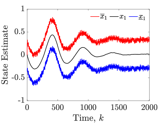
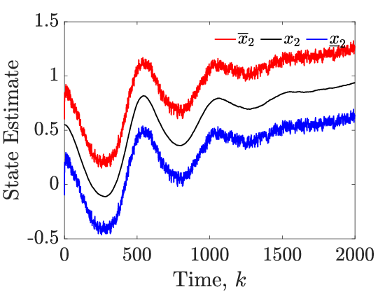
Figure 1: Actual states, $x_{1,k}$, $x_{2,k}$, as well as their corresponding upper and lower framers outputted by the proposed observer (23), $\overline{x}_{1,k}$, $\underline{x}_{1,k}$, $\overline{x}_{2,k}$, $\underline{x}_{1,k}$ in a horizon of $K=2000$ time steps.

Figure 1 shows the interval framers of the states, obtained by applying the proposed observer in (23) in a horizon of $K=2000$ time steps. For the sake of comparison, we also applied our previous approach in [26] which is based on computing affine over-approximation of the nonlinear dynamics at each time step, and hence, requires running computationally expensive online optimizations. While the newly proposed approach took only $0.195287$ seconds to run and returned the framers, the one in [26] failed to provide results in a timely manner, i.e, we had to terminate it manually after almost ten hours.

Furthermore, as can be seen in Figure 2, only after we reduced the horizon to $K=250$ time steps, we observed that our previous approach in [26] returned estimates $\underline{x}^{\text{MZ}}_{k},\overline{x}^{\text{MZ}}_{k}$, which were tighter than the ones outputted by the method in this paper, i.e., $\underline{x}_{k},\overline{x}_{k}$. However, even for this shorter time horizon, it took $1080.79$ seconds (almost three hours) for the approach in [26] to return the results, while the computation time for the new approach was only $0.1201$ seconds.

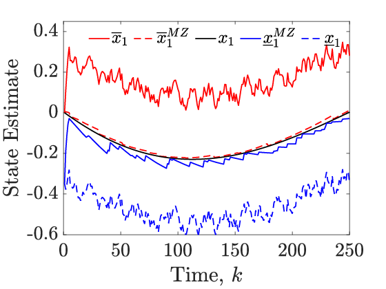
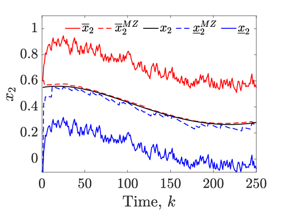
Figure 2: Actual state, $x_{k}$, as well as its estimated framers, outputted by the proposed observer (23), $\overline{x}_{1,k}$, $\underline{x}_{1,k}$, $\overline{x}_{2,k}$, $\underline{x}_{2,k}$ in addition to the state framers obtained from the approach in [26], $\overline{x}^{\text{MZ}}_{1,k}$, $\underline{x}^{\text{MZ}}_{1,k}$, $\overline{x}^{\text{MZ}}_{2,k}$, $\underline{x}^{\text{MZ}}_{2,k}$, in a horizon of $K=250$ time steps.

Finally, Figure 3 shows the framer intervals of the learned/estimated unknown dynamics model that frame the actual unknown dynamics function $h$, i.e., satisfies (16), as well as the global (affine) function approximation, computed via [26, Proposition 2] at the initial step.

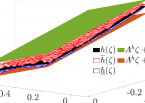
Figure 3: Actual unknown dynamics function $h(\zeta)$, its upper and lower framer intervals $\overline{h}_{k},\underline{h}_{k}$ at time step $k=250$, as well as its global abstraction $A^{h}\zeta+\overline{e}^{h},A^{h}\zeta+\underline{e}^{h}$ via [26, Proposition 2] at the initial step.

VI Conclusion & Future Work

In this paper, the problem of synthesizing interval observers for partially unknown nonlinear systems with bounded noise was addressed, aiming to simultaneously estimate system states and learn a model of the unknown dynamics. A framework was developed by leveraging Jacobian sign-stable (JSS) decompositions, tight decomposition functions for nonlinear systems, and a data-driven over-approximation approach, enabling the recursive computation of interval estimates that were proven to enclose the true augmented states. Tight and tractable bounds for the unknown dynamics were constructed as functions of current and past interval framers, allowing for their systematic integration into the observer design. Furthermore, semi-definite programs (SDP) were formulated to synthesize observer gains, ensuring input-to-state stability and optimality of the proposed design. Finally, simulation results demonstrated that the proposed approach outperformed the method in [26] in terms of computational efficiency. Future work will consider (partially) unknown continents-time and hybrid dynamical systems.

References

- [1] W. Liu and I. Hwang. Robust estimation and fault detection and isolation algorithms for stochastic linear hybrid systems with unknown fault input. IET control theory & applications, 5(12):1353–1368, 2011.
- [2] S.Z. Yong, M. Zhu, and E. Frazzoli. Switching and data injection attacks on stochastic cyber-physical systems: Modeling, resilient estimation and attack mitigation. ACM Transactions on Cyber-Physical Systems, 2(2):9, 2018.
- [3] S.Z. Yong. Simultaneous input and state set-valued observers with applications to attack-resilient estimation. In 2018 Annual American Control Conference (ACC), pages 5167–5174. IEEE, 2018.
- [4] L. Jaulin. Nonlinear bounded-error state estimation of continuous-time systems. Automatica, 38(6):1079–1082, 2002.
- [5] M. Kieffer and E. Walter. Guaranteed nonlinear state estimator for cooperative systems. Numerical algorithms, 37(1-4):187–198, 2004.
- [6] M. Moisan, O. Bernard, and J-L. Gouzé. Near optimal interval observers bundle for uncertain bioreactors. In European Control Conference (ECC), pages 5115–5122. IEEE, 2007.
- [7] O. Bernard and J-L. Gouzé. Closed loop observers bundle for uncertain biotechnological models. Journal of Process Control, 14(7):765–774, 2004.
- [8] T. Raïssi, G. Videau, and A. Zolghadri. Interval observer design for consistency checks of nonlinear continuous-time systems. Automatica, 46(3):518–527, 2010.
- [9] T. Raïssi, D. Efimov, and A. Zolghadri. Interval state estimation for a class of nonlinear systems. IEEE Transactions on Automatic Control, 57(1):260–265, 2011.
- [10] F. Mazenc and O. Bernard. Interval observers for linear time-invariant systems with disturbances. Automatica, 47(1):140–147, 2011.
- [11] F. Mazenc, T-N. Dinh, and S-I. Niculescu. Robust interval observers and stabilization design for discrete-time systems with input and output. Automatica, 49(11):3490–3497, 2013.
- [12] Y. Wang, D-M. Bevly, and R. Rajamani. Interval observer design for LPV systems with parametric uncertainty. Automatica, 60:79–85, 2015.
- [13] D. Efimov, T. Raïssi, S. Chebotarev, and A. Zolghadri. Interval state observer for nonlinear time varying systems. Automatica, 49(1):200–205, 2013.
- [14] G. Zheng, D. Efimov, and W. Perruquetti. Design of interval observer for a class of uncertain unobservable nonlinear systems. Automatica, 63:167–174, 2016.
- [15] F. Mazenc, T.N. Dinh, and S.I. Niculescu. Interval observers for discrete-time systems. International journal of robust and nonlinear control, 24(17):2867–2890, 2014.
- [16] N. Ellero, D. Gucik-Derigny, and D. Henry. An unknown input interval observer for LPV systems under -gain and -gain criteria. Automatica, 103:294–301, 2019.
- [17] M. Khajenejad and S.Z. Yong. Simultaneous input and state set-valued -observers for linear parameter-varying systems. In American Control Conference (ACC), pages 4521–4526. IEEE, 2019.
- [18] M. Khajenejad and S.Z. Yong. Simultaneous mode, input and state set-valued observers with applications to resilient estimation against sparse attacks. In 2019 IEEE 58th Conference on Decision and Control (CDC), pages 1544–1550. IEEE, 2019.
- [19] M. Khajenejad and S.Z. Yong. Simultaneous state and unknown input set-valued observers for nonlinear dynamical systems. arXiv preprint arXiv:2001.10125, Submitted to Automatica, under review, 2020.
- [20] M. Khajenejad and S.Z. Yong. Simultaneous input and state interval observers for nonlinear systems with full-rank direct feedthrough. arXiv preprint arXiv:2002.04761, Accepted in CDC, 2020.
- [21] M. Milanese and C. Novara. Set membership identification of nonlinear systems. Automatica, 40:957–975, 2004.
- [22] M. Canale, L. Fagiano, and M.C. Signorile. Nonlinear model predictive control from data: a set membership approach. International Journal of Robust and Nonlinear Control, 24(1):123–139, 2014.
- [23] Z.B Zabinsky, R.L Smith, and B.P Kristinsdottir. Optimal estimation of univariate black-box Lipschitz functions with upper and lower error bounds. Computers & Operations Res., 30(10):1539–1553, 2003.
- [24] G. Beliakov. Interpolation of Lipschitz functions. Journal of computational and applied mathematics, 196(1):20–44, 2006.
- [25] J.P. Calliess. Conservative decision-making and inference in uncertain dynamical systems. PhD thesis, University of Oxford, 2014.
- [26] M. Khajenejad, Z. Jin, and S.Z. Yong. Interval observers for simultaneous state and model estimation of partially known nonlinear systems. In 2021 American Control Conference (ACC), pages 2848–2854. IEEE, 2021.
- [27] Z. Jin, M. Khajenejad, and S.Z. Yong. Data-driven model invalidation for unknown lipschitz continuous systems via abstraction. In American Control Conference (ACC), pages 2975–2980. IEEE, 2020.
- [28] M. Khajenejad, F. Shoaib, and S.Z. Yong. Interval observer synthesis for locally Lipschitz nonlinear dynamical systems via mixed-monotone decompositions. In 2022 American Control Conference (ACC), pages 2970–2975. IEEE, 2022.
- [29] L. Yang, O. Mickelin, and N. Ozay. On sufficient conditions for mixed monotonicity. IEEE Transactions on Automatic Control, 64(12):5080–5085, 2019.
- [30] M.C. De Oliveira, J.C. Geromel, and J. Bernussou. Extended and norm characterizations and controller parameterizations for discrete-time systems. Int. J. of Control, 75(9):666–679, 2002.
- [31] T. Pati, M. Khajenejad, and S.Z Yong. Computationally efficient and optimal interval observer design. In European Control Conference (ECC), accepted. https://sites.google.com/view/mohammad-khajenejad/publications?authuser=0, 2025.
- [32] Dimitrios Pylorof, Efstathios Bakolas, and Kevin S Chan. Design of robust lyapunov-based observers for nonlinear systems with sum-of-squares programming. IEEE Control Systems Letters, 4(2):283–288, 2019.
- [33] J. Löfberg. YALMIP: A toolbox for modeling and optimization in MATLAB. In CACSD, Taipei, Taiwan, 2004.