Gradient-based Sample Selection for Faster Bayesian Optimization

Abstract

Bayesian optimization (BO) is an effective technique for black-box optimization. However, its applicability is typically limited to moderate-budget problems due to the cubic complexity in computing the Gaussian process (GP) surrogate model. In large-budget scenarios, directly employing the standard GP model faces significant challenges in computational time and resource requirements. In this paper, we propose a novel approach, gradient-based sample selection Bayesian Optimization (GSSBO), to enhance the computational efficiency of BO. The GP model is constructed on a selected set of samples instead of the whole dataset. These samples are selected by leveraging gradient information to maintain diversity and representation. We provide a theoretical analysis of the gradient-based sample selection strategy and obtain explicit sublinear regret bounds for our proposed framework. Extensive experiments on synthetic and real-world tasks demonstrate that our approach significantly reduces the computational cost of GP fitting in BO while maintaining optimization performance comparable to baseline methods.

1 Introduction

Bayesian optimization (BO) (Frazier, 2018) is a successful approach to black-box optimization that has been applied in a wide range of applications, such as hyperparameter optimization, reinforcement learning, and mineral resource exploration. BO’s strength lies in its ability to represent the unknown objective function through a surrogate model and by optimizing an acquisition function (Garnett, 2023; Wang et al., 2023). BO consists of a surrogate model, which provides a global predictive model for the unknown objective function, and an acquisition function that serves as a criterion to strategically determine the next sample to evaluate. In particular, the Gaussian process (GP) model is often preferred as the surrogate model due to its versatility and reliable uncertainty estimation. However, the GP model often suffers from large data sets, making it more suitable for small-budget scenarios (Binois & Wycoff, 2022). To fit a GP model, the dominant complexity in computing the inversion of the covariance matrix inversion is $\mathcal{O}(n^{3})$, where $n$ is the number of data samples. As the sample set grows, the computational burden increases substantially. This limitation poses a significant challenge for scaling BO to real-world problems with large sample sets.

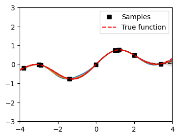
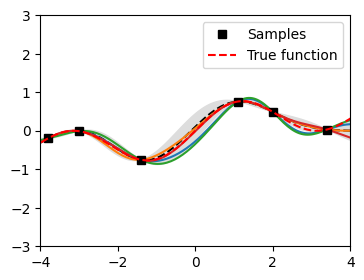
Figure 1: Illustration of GP fitting with sample selection. Left: GP fitted with 10 samples. Right: GP fitted with 6 selected samples. With fewer selected samples, we can still fit a good GP to estimate the black box function, which can also guide us in finding the global optimum.

Despite the various approaches in improving the computational efficiency of BO, including parallel BO (González et al., 2016; Daulton et al., 2021, 2020; Eriksson et al., 2019), kernel approximation methods (Kim et al., 2021; Jimenez & Katzfuss, 2023; Hensman et al., 2013; Williams & Seeger, 2000) and sparse GP (Lawrence et al., 2002; Leibfried et al., 2020; McIntire et al., 2016), the computational overhead can still become a burden in practice. Current implementations of sparse GPs (McIntire et al., 2016) for BO adopt iterative schemes that add a new sample while removing one from the original subset at each iteration. Although this approach reduces computational complexity, it can be suboptimal in identifying the most representative subset, especially in complex optimization landscapes. Furthermore, while BO algorithms are theoretically designed to balance exploitation and exploration, with limited budget in practice, they can over-exploit current best regions before shifting to exploration Wang & Ng (2020), leading to suboptimal performance in locating the global optimums.

During the iterative search process of BO, some samples can become redundant and contribute little to the additional information gain. Such samples collected in earlier stages thus diminish in importance as the process evolves. For instance, excessive searching around identified minima becomes redundant once the optimal value has been determined, as these samples cease to offer meaningful insights for further optimization. To efficiently fit a GP, it is essential to focus on samples that provide the most informative contributions. As shown in Figure 1, carefully selected samples can effectively fit a GP. Despite the reduced number of samples, the GP still captures the key trends and features of the true function while maintaining reasonable uncertainty bounds. In this paper, we propose to incorporate the gradient-based sample selection technique into the BO framework to enhance its scalability and effectiveness in large-budget scenarios. This technique was originally proposed for continuing learning with online data stream (Aljundi et al., 2019). The previously seen data are selectively sampled and stored in a replay buffer to prevent catastrophic forgetting and enhance model fitting. The iterative optimization process of BO can be viewed as an online data acquiring process. Hence, the GP model fitting in the next iteration can be seen as a similar continuing learning problem. By using gradient information to gauge the value of each sample, one can more judiciously decide which samples are most essential for building a subset, and maintain the most representative subset of BO samples. This subset is then used to fit the GP model, accelerating the BO process while ensuring efficient and effective GP fitting and mitigating the problem of over-exploitation. We summarize our main contributions as follows:

• Efficient computations. We propose Gradient-based Sample Selection Bayesian Optimization (GSSBO) that addresses the scalability challenges associated with large-budget scenarios. Our approach is an out-of-the-box algorithm that can seamlessly integrate into existing BO frameworks with only a small additional computational overhead.

• Theoretical analysis. We provide a rigorous theoretical analysis of the regret bound for the GSSBO. Theoretical results show that the regret bound of the proposed algorithm (with sample selection) is similar to that of the standard GP-UCB algorithm (without sample selection).

• Empirical validations. We conduct comprehensive numerical experiments, including synthetic and real-world datasets, to demonstrate that compared to baseline methods, the proposed algorithm achieves comparable performance, but significantly reduces computational costs. These results verify the benefit of using gradient information to select a representative subset of samples.

2 Related Works

BO with Resource Challenges. In practical applications, BO faces numerous challenges, including high evaluation costs, input-switching costs, resource constraints, and high-dimensional search spaces. Researchers have proposed a variety of methods to address these issues. For instance, parallel BO employs batch sampling to improve efficiency in large-scale or highly concurrent scenarios (González et al., 2016; Daulton et al., 2021, 2020; Eriksson et al., 2019). Kernel approximation methods, such as random Fourier features, map kernels onto lower-dimensional feature spaces, thus accelerating kernel-based approaches (Rahimi & Recht, 2007; Kim et al., 2021). Multi-fidelity BO leverages coarse simulations together with a limited number of high-fidelity evaluations to reduce the overall experimental cost (Kandasamy et al., 2016). For high-dimensional tasks, techniques such as random embeddings or active subspaces help reduce the search dimensionality (Wang et al., 2016). Meanwhile, sparse GP significantly reduces computational complexity by introducing “inducing points” (Lawrence et al., 2002; Leibfried et al., 2020; McIntire et al., 2016). However, these methods face limitations in practical usage scenarios, often struggling to balance complex resource constraints while dynamically adapting to high-dimensional and rapidly changing environments.

BO with Gradient Information. The availability of derivative information can significantly simplify optimization problems. Ahmed et al. (2016) highlight the potential of incorporating gradient information into BO methods and advocate for its integration into optimization frameworks. Wu & Frazier (2016) introduced the parallel knowledge gradient method for batch BO, achieving faster convergence to global optima. Rana et al. (2017) incorporated GP priors to enable gradient-based local optimization. Chen et al. (2018) proposed a unified particle-optimization framework using Wasserstein gradient flows for scalable Bayesian sampling. Bilal et al. (2020) demonstrated that BO with gradient-boosted regression trees performed well in cloud configuration tasks. Tamiya & Yamasaki (2022) developed stochastic gradient line BO (SGLBO) for noise-robust quantum circuit optimization. Penubothula et al. (2021) funded local critical points by querying where the predicted gradient is zero. Zhang & Rodgers (2024) introduced BO of gradient trajectory (BOGAT) for efficient imaging optimization. Although these methods leverage gradient information to improve optimization efficiency and performance, they mainly focus on refining the GP model or acquisition functions.

Subset Selection. Subset selection is a key task in fields such as regression, classification, and model selection, aiming to improve efficiency by selecting a subset of features or data. Random subset selection, a simple and widely used method, involves randomly sampling data, often for cross-validation or bootstrap (Hastie, 2009). Importance-based selection focuses on high-value data points, while active learning targets samples that are expected to provide the most information, improving model learning (Quinlan, 1986). Filter methods rank features using statistical measures such as correlation or variance, selecting the top-ranked ones for modeling (Guyon & Elisseeff, 2003). Narendra & Fukunaga (1977) introduced a branch-and-bound algorithm for efficient feature selection, and Wei et al. (2015) proposed filtering active submodular selection (FASS), combining uncertainty sampling with submodular optimization. Yang et al. (2022) proposed dataset pruning, an optimization-based sample selection method that identifies the smallest subset of training data to minimize generalization gaps while significantly reducing training costs. Zhu (2016) proposed an efficient method to approximate the gradient of the objective function using a pilot estimate. The core idea is to compute the gradient information corresponding to each data point based on an initial parameter estimate (referred to as the “pilot estimate”) and identify data points with larger gradient values as more “important” samples for subsequent optimization. Despite these advancements, directly applying subset selection methods to BO often yields suboptimal results, necessitating further exploration to integrate subsampling effectively into BO frameworks.

3 Background

3.1 Bayesian Optimization and Gaussian Processes

BO aims to find the global optimum $x^{*}\in\mathcal{X}$ of an unknown reward function $f:\mathcal{X}\to\mathbb{R}$, over the $n$-dimensional input space $\mathcal{X}=[0,1]^{n}$. Throughout this paper, we consider minimization problems, i.e., we aim to find $x^{*}\in\mathcal{X}$ such that $f(x^{*})\leq f(x)$ for all $x\in\mathcal{X}$, approximating the performance of the optimal point $x^{*}=\arg\max_{x\in\mathcal{X}}f(x)$ as quickly as possible. GPs are one of the fundamental components in BO, providing a theoretical framework for modeling and prediction in a black-box function. In each round, a sample $x_{t}$ is selected based on the current GP’s posterior and acquisition function. The observed values $y_{t}$ and $x_{t}$ are then stored in the sample buffer, and the GP surrogate is updated according to these samples. This iterative process of sampling and updating continues until the optimization objects are achieved or the available budget is exhausted.

The key advantage of GPs lies in their nonparametric nature, allowing them to model complex functions without assuming a specific form. GPs are widely used for regression (Gaussian Process Regression (Schulz et al., 2018), GPR) and classification tasks due to their flexibility and ability to provide uncertainty estimates. Formally, a GP can be defined as: $f(\mathbf{x})\sim\mathcal{GP}(\mu(x),k(x,x^{\prime})))$, where $\mu(x)$ is the mean function, often assumed to be zero, and $k(x,x^{\prime})$ is the covariance function, defining the similarity between points $x$ and $x^{\prime}$. It should be noted that the algorithmic complexity of GP updates is $\mathcal{O}(n^{3})$, where $n$ is the number of observed samples. As the sample set grows, the computational resources required for these updates can become prohibitively expensive, especially in large-scale optimization problems.

3.2 Diversity-based Subset Selection

Due to limited computing resources, intelligently selecting samples instead of using all samples to fit a model is more efficient in problems with a large sample set. In continuing learning, this will overcome the catastrophic forgetting of previously seen data when faced with online data streams. Suppose that we have a model fitted on observed samples $\mathcal{D}\triangleq\{(x_{1},y_{1}),\ldots,(x_{n},y_{n})\}$, where $x_{i}\in\mathcal{X}$ and $y_{i}$ is the corresponding observation. In the context of subset selection, our objective is to ensure that each newly added sample contributes meaningfully to the optimization process; that is, the goal of sequential selecting the sample is to minimize the loss function $\ell(f(x_{n};\theta),y_{n})$, where $f(\cdot;\theta)$ denotes the model parameterized by $\theta$. Formally, this can be expressed as:

$$\begin{split}\theta^{n}&=\arg\min_{\theta}\ell(f(x_{n};\theta),y_{n})\\ \text{s.t.}\quad&\ell(f(x_{i};\theta),y_{i})\leq\ell(f(x_{i};\theta^{n-1}),y_{i}),\,\\ &\forall i\in\{1,\dots,n-1\}.\end{split}$$ (1)

The constraints ensure that when we select new samples for the sample subset, the loss of the new samples will not exceed that of the previous subset samples, thereby preserving the performance of the previously observed subset.

Let $g_{n}=\nabla_{\theta}\ell(f(x_{n};\theta),y_{n})$ be the gradient of loss for model parameters $\theta$ at time $n$. Following Aljundi et al. (2019), we rephrase the constraints involving the loss with respect to the gradients. Specifically, the constraint of (1) can be rewritten as $\langle\mathbf{g}_{n},\mathbf{g}_{i}\rangle\geq 0,\forall i\in\{1,\dots,n-1\}.$ This transformation simplifies the constraint by focusing on the inner product of the gradients, which are nonnegative such that the loss does not increase.

To solve (1), we consider the geometric properties of the gradients in the parameter space. Note that optimizing the solid angle subtended by the gradients is computationally expensive. According to the derivation in Aljundi et al. (2019), the sample selection problem is equivalent to maximizing the variance of the loss gradient direction of the samples in the fixed-size buffer. By maximizing the variance of the gradient directions, we ensure that the selected samples represent diverse regions of the parameter space, and therefore the buffer contains diverse samples, each contributing unique information to the optimization process. How to determine the buffer size will be detailed in Section 4.3. Problem (1) thus becomes a surrogate of selecting a subset $\mathcal{U}$ of the samples that maximize the diversity of their gradients:

$$\text{Var}_{\mathcal{U}}\left[\frac{\mathbf{g}}{\|\mathbf{g}\|}\right]=1-\frac{1}{M^{2}}\sum_{i,j\in\mathcal{U}}\frac{\langle\mathbf{g}_{i},\mathbf{g}_{j}\rangle}{\|\mathbf{g}_{i}\|\|\mathbf{g}_{j}\|}.$$ (2)

Here, $M$ denotes the number of samples saved in the buffer and $\textbf{g}/\|\textbf{g}\|$ is the normalized gradient vector. The reformulated problem (2) transforms the sample selection process from a sequential approach (adding samples to the subset one at a time) into a batch selection approach (samples are selected all at once).

4 Bayesian Optimization with Gradient-based Sample Selection

4.1 Gradient Information with GP

In light of the pilot estimate-based gradient information acquisition method in Zhu (2016), we propose a new method for gradient information acquisition in GPs. In a GP model, given a set of samples $\mathcal{D}=\{(x_{1},y_{1}),\ldots,(x_{n},y_{n})\}$ that follows a multivariate normal distribution with mean $\mu$ and covariance matrix $\mathbf{K}$, where $\mathbf{K}$ is constructed from a kernel function $k(\mathbf{x}_{i},\mathbf{x}_{j};\theta)$ and ${\theta}$ represents the hyperparameters, the probability density function of a multivariate Gaussian distribution is $p(\mathbf{y}|\mathbf{X},{\theta})=\frac{1}{(2\pi)^{n/2}|\mathbf{K}|^{1/2}}\exp\left(-\frac{1}{2}\mathbf{(y-\mu)}^{T}\mathbf{K}^{-1}\mathbf{(y-\mu)}\right)$.Taking logarithm on it and we derive the log-likelihood function:

$$\begin{split}\log p(\mathbf{y}|\mathbf{X},{\theta})=&-\frac{1}{2}\mathbf{(y-\mu)}^{T}\mathbf{K}^{-1}\mathbf{(y-\mu)}\\ &-\frac{1}{2}\log|\mathbf{K}|-\frac{n}{2}\log(2\pi).\end{split}$$ (3)

Remark 4.1.

The log-likelihood function in (3) comprises three terms. The first term, $-\frac{1}{2}\mathbf{(y-\mu)}^{T}\mathbf{K}^{-1}\mathbf{(y-\mu)}$, represents the sample fit under the covariance structure specified by $\mathbf{K}$. The second term, $-\frac{1}{2}\log|\mathbf{K}|$, penalizes model complexity through the log-determinant of the covariance matrix. The third term, $-\frac{n}{2}\log(2\pi)$, is a constant to the parameters and thus does not affect the gradient calculation.

The derivative of $\mathbf{y}$ directly measures how sensitive this log-likelihood is to each observation $y_{i}$. Intuitively, if changing $y_{i}$ significantly alters the value of (3), that sample has a large marginal contribution to the fit. Hence, in subset selection schemes, one can use these gradient magnitudes to gauge how important each sample is, potentially adjusting their weights or deciding which samples to retain in a subset.

To define the gradient for each sample, we first quantify each sample’s contribution to the log-likelihood. Since the second and third terms in (3), $-\frac{1}{2}\log|\mathbf{K}|$ and $-\frac{n}{2}\log(2\pi)$, do not depend on $\mathbf{y}$, both have no contribution to the gradient. Consequently, the gradient of the log-likelihood with respect to $\mathbf{y}$ is given by: $\frac{\partial\log p(\mathbf{y|X},{\theta})}{\partial\mathbf{y}}=-\mathbf{K}^{-1}(\mathbf{y}-\mu)$. Note that the $i$-th component, $-(\mathbf{K}^{-1}(\mathbf{y}-\mu))_{i}$, corresponds to the partial derivative of the log-likelihood with respect to $\mathbf{y}_{i}$. Thus, we define the gradient $g_{i}$ for each sample $\mathbf{y}_{i}$ as:

$$g_{i}=\frac{\partial\log p(\mathbf{y|X},{\theta})}{\partial\mathbf{y}}=-(\mathbf{K}^{-1}(\mathbf{y}-\mu))_{i}.$$ (4)

This gradient calculation is computationally efficient as the value of $\mathbf{K}^{-1}$ in (4) is available while updating the GP. Furthermore, the complexity of the additional computational burden introduced by the gradient calculation is $O(n^{2})$, and it is negligible to the complexity of GP updates (which is $O(n^{3})$), especially when $n$ is large.

4.2 Gradient-based Sample Selection

As the number of observed samples increases, fitting a GP model can become prohibitively expensive, especially in large-scale scenarios. A common remedy is to work with a subset of samples of size $M\ll N$, thereby reducing the computational cost of GP updates. Once the kernel parameters are fixed, the efficiency and effectiveness of GP model fitting in BO are closely related to the quality of this chosen subset. This raises the question: How do we choose a subset that remains representative and informative?

Inspired by the success of gradient-based subset selection methods in machine learning, we propose leveraging gradient information to guide the selection of such subsets within BO. To this end, we introduce a gradient-based sample selection methodology to ensure representativeness within a limited sample buffer size. By harnessing gradient information, our approach maintains a carefully chosen subset of samples that not only eases computational burdens, but also preserves model quality, even as the sample set size grows.

We begin by modeling the objective function $f$ with a GP and setting a buffer size $M$. Initially, the algorithm observes $f$ at $n_{0}$ samples, retaining these initial samples to preserve global information critical to the model. After each subsequent evaluation, if the number of samples exceeds $M$, we perform a gradient-based sample selection step to ensure that only $M$ representative samples are kept for the next GP update.

4.3 Gradient-based Sample Selection BO

The following outlines the GSSBO implementation details and considerations to improve the optimization process, effectively addressing practical challenges. We highlight the key insight of this subsection: we tackle the scalability of BO by maintaining a subset of the most representative and informative samples that are selected based on gradient information.

Detailed Implementations. In the initialization phase, $n_{0}$ initial samples $\{(x_{i},y_{i})\}_{i=1}^{n_{0}}$ are observed; and the initial sample set $D$, the buffer size $M$, and total budget $N$ are specified. In each iteration, the GP posterior is updated based on the current sample set $D$; an acquisition function (e.g., UCB) is built to select the next point $x_{t}$, and the corresponding observation $y_{t}=f(x_{t})$ is obtained; and the sample $(x_{t},y_{t})$ is added to $D$. To manage each iteration’s computational complexity, a buffer check and gradient-based selection step are performed. Specifically, if the current size of $D$ is less than or equal to $M$, the GP is updated using all samples in $D$. Otherwise, a gradient-based sample selection step is performed to identify a set of the most representative samples. Note that the $n_{0}$ initial samples and the newly acquired sample $(x_{t},y_{t})$ are always added into the subset, as they provide base information for the GP model and ensure that recently observed information is always retained, respectively. Besides the initial $n_{0}$ and the newly observed samples, $(M-n_{0}-1)$ samples are selected by minimizing the sum of pairwise cosine similarities among their gradients. The resulting subset $\mathcal{U}$, containing $M$ samples, is then used to fit the GP model. The complete procedure is outlined in Algorithm 4.3.

(1) Dynamic Buffer Size. In practice, the buffer size should be prespecified by the users. However, the value is often unavailable in advance. Instead, we propose a dynamic adjustment mechanism to determine the buffer size. We define a tolerable maximum factor $Z$ to accelerate GP computations. Let $\bar{T}$ be the average evaluation time for a single sample point estimated based on the initial iterations and $T_{\text{current}}$ be the current iteration’s computation time. If $T_{\text{current}}$ exceeds the user-specified threshold $Z\times\bar{T}$, the buffer size is set to be the number of all current samples, i.e., $M=|D|$. This adaptive strategy ensures that the algorithm balances computational efficiency with the goal of utilizing as much data as possible, thereby maintaining high predictive accuracy without incurring excessive costs.

(2) Preserving Initial Samples and Latest Observations. During the procedure, the initial $n_{0}$ samples are always included in the subset. These samples capture essential information about the overall function landscape, and good initialization samples give us useful information about the global situation. Additionally, the newly acquired sample, $(x_{t},y_{t})$, is also included in the subset. This ensures that the GP model incorporates the latest data, maintaining its relevance and accuracy. Consequently, the algorithm prevents valuable information from being prematurely excluded. Additionally, this essentially alleviates a limitation of sparse GP in BO (McIntire et al., 2016): the constrained representation size may hinder the full integration of new observations into the model.

(3) Random Perturbation to Escape Local Optima. Subset selection may cause the algorithm to become trapped in the local optima, as it iteratively selects a subset of “locally optimal” samples. This issue arises when certain samples are frequently chosen by the acquisition function but consistently excluded from the sample subset, hindering the exploration of other valuable samples. To address this issue, Gaussian noise $\epsilon_{i}\sim\mathcal{N}(0,\sigma^{2})$ is added to each computed gradient $g_{i}$, resulting in perturbed gradients $\tilde{g}_{i}=g_{i}+\epsilon_{i}$. This perturbation introduces variability into the gradient-based selection process, helping the algorithm escape local optima and facilitating the exploration of a more diverse set of samples. The parameter $\sigma$ serves as a tunable control for the degree of perturbation.

 

Algorithm 1 Gradient-based Sample Selection BO

 

1: Initialization: Place a GP prior on $f$. Obtain $n_{0}$ initial samples $D=\{(x_{i},y_{i})\}_{i=1}^{n_{0}}$. Set the buffer size $M>n_{0}$, total budget $N$, and average initial iteration time $\bar{T}$.

2: for $t=n_{0}+1$ to $N$ do

3:  Update posterior $p(f\mid D)$.

4:  Select $x_{t}=\arg\max_{x}\alpha(x;p(f|D))$, where $\alpha$ is the acquisition function.

5:  Evaluate $y_{t}=f(x_{t})$ and set $D=D\cup\{(x_{t},y_{t})\}$.

6:  if $|D|>M$ then

7:   Compute gradients $g_{i}$ for samples $(x_{i},y_{i})\in D$.

8:   Add the newest sample $(x_{t},y_{t})$ into the subset.

9:   Form a subset $\mathcal{U}$ by forcing in the $n_{0}$ initial samples and the newest sample $(x_{t},y_{t})$.

10:   Select $(M-n_{0}-1)$ samples from $D$ such that the sum of $\{\tilde{g}_{i}\}$ is minimized.

11:   Update the GP using the $M$ selected samples.

12:  else

13:   Update the GP using all samples in $D$.

14:  end if

15:  Let $T_{\text{current}}$ be the current iteration time.

16:  if $T_{\text{current}}>Z\times\bar{T}$ then

17:   Set $M=|D|$.

18:  end if

19: end for

 

5 Theoretical Analysis

Gaussian Process Upper Confidence Bound (GP-UCB (Srinivas et al., 2009)) is a popular algorithm for sequential decision-making problems. We propose an extension to GP-UCB by incorporating gradient-based sampling. In this section, we analyze the error of the subset fitted GP and prove that the regret of the GSSBO with GP-UCB algorithm is bounded.

Theorem 5.1.

(Error in the Subset-Fitted GP) This theorem establishes bounds on the difference between the posterior mean and variance under a subset fitted GP approximation and those of the full set fitted GP. Given a GP with kernel matrix $\mathbf{K}_{\mathcal{D}\mathcal{D}}$, a low-rank approximation $\hat{\mathbf{K}}=\mathbf{K}_{\mathcal{D}\mathcal{U}}\mathbf{K}_{\mathcal{U}\mathcal{U}}^{-1}\mathbf{K}_{\mathcal{U}\mathcal{D}}$ constructed from $M$ inducing samples and a test sample $\mathbf{x}_{*}$, the posterior predictive mean and variance errors satisfy:

$$|\Delta\mu(\mathbf{x}_{*})|\leq\|\mathbf{k}_{*\mathcal{D}}\|\|\mathbf{y}\|C_{1}\|\mathbf{K}_{\mathcal{D}\mathcal{D}}-\hat{\mathbf{K}}\|,$$

$$|\Delta\sigma^{2}(\mathbf{x}_{*})|\leq\|\mathbf{k}_{*\mathcal{D}}\|^{2}C_{1}\|\mathbf{K}_{\mathcal{D}\mathcal{D}}-\hat{\mathbf{K}}\|,$$

where $\mathbf{k}_{*\mathcal{D}}\in\mathbb{R}^{N}$ means the covariance vector between the test sample $\mathbf{x}_{*}$ and all training samples in $\mathcal{D}$, $C_{1}=\|({\mathbf{K}_{\mathcal{D}\mathcal{D}}+\sigma_{n}^{2}\mathbf{I}})^{-1}\|\|({\hat{\mathbf{K}}+\sigma_{n}^{2}\mathbf{I}})^{-1}\|$.

To aid in the theoretical analysis, we make the following assumptions.

Assumption 5.1. Assume there exist constants $a$, $b$, and $L$ such that the kernel function $k(\mathbf{x},\mathbf{x}^{\prime})$ satisfies a Lipschitz continuity condition, providing confidence bounds on the derivatives of the GP sample paths $f$:

$$P\left(\sup_{\mathbf{x}\in\mathcal{X}}\left|\frac{\partial f}{\partial x_{j}}\right|>L\right)\leq ae^{-L^{2}/b^{2}}\quad\text{for }j=1,\ldots,p.$$

A typical example of such a kernel is the squared exponential kernel $k(\mathbf{x},\mathbf{x}^{\prime})=\sigma^{2}\exp\left(-\frac{\|\mathbf{x}-\mathbf{x}^{\prime}\|^{2}}{2l^{2}}\right)$, where $l$ is the length-scale parameter and $\sigma^{2}$ represents the noise variance. Then we propagate the error in Theorem 5.1 through the GP posterior to bound the GSSBO regret.

Theorem 5.2.

(Regret Bound for GSSBO with UCB) Let $\mathcal{X}\subseteq[0,r]^{p}$ be compact and convex, $p\in\mathbb{N},r>0$, let $A=\|\mathbf{k}_{*\mathcal{D}}\|\|\mathbf{y}\|\;C_{1}\,(\lambda_{M+1}+\epsilon\sum_{i=1}^{N}(\mathbf{K}_{\mathcal{D}\mathcal{D}})_{ii}^{2})$, $\delta\geq A/\sigma_{\min}$. Under Assumption 1, for any arbitrarily small $\delta\in(0,1)$, choose

$$\beta_{n}=2\log\frac{4\pi_{n}}{\delta}+{2p}\log\left(n^{2}brp\sqrt{\log\left(\frac{4pa}{\delta}\right)}\right)-\frac{A}{\sigma_{\min}},$$

where $\sum_{n\geq 1}\pi_{n}^{-1}=1,\pi_{n}>0$. As $n\to\infty$, we obtain a regret bound of $\mathcal{O}^{*}\left(\sqrt{pN\gamma_{N}}\right)$. Specifically, with $C=\frac{8}{\log(1+\sigma^{-2})},$ we have:

$$P\left(R_{N}\leq\sqrt{CN\beta_{N}\gamma_{N}}\right)\geq 1-\delta.$$

(Two-Phase Regret) Let $N$ be the total number of rounds. In the first $M_{\text{initial}}$ rounds, one applies the full GP-UCB. Subsequently, from round $M+1$ to $N$, one switches to the gradient-based subset strategy. The total regret satisfies $R_{N}\;=\;R_{M}^{(\text{full})}\;+\;R_{N-M}^{(\text{selected})},$ where $R_{M}^{(\text{full})}\leq\sqrt{\,C\,M\,\beta_{M}\,\gamma_{M}+2}$ and $R_{N-M}^{(\text{selected})}\leq\sqrt{\,C\,(N-M)\,\beta_{(N-M)}\,\gamma_{(N-M)}}$.

The sketch proof for the main theorem is relegated to the Appendix.

The main theoretical challenge lies in evaluating the error between the low-rank approximation $\hat{\mathbf{K}}$ and the full $\mathbf{K}_{\mathcal{D}\mathcal{D}}$. By invoking spectral norm inequalities and the Nyström approximation theory, $\|\mathbf{K}_{\mathcal{D}\mathcal{D}}-\hat{\mathbf{K}}\|$ can be bounded. Then, we merge the resulting linear and $\beta$-scaled error terms into a single penalty in the UCB construction. This establishes a regret bound for GSSBO, which is similar to that of classical GP-UCB. From a practical relevance perspective, Theorem 5.1 indicates that limiting the GP to a smaller, well-chosen subset does not substantially degrade posterior accuracy in either the mean or variance estimates. Restricting the subset size $M$ confers significant computational savings while ensuring performance closely matches that of a standard GP-UCB using all samples. Of note, we also observe that, compared with the classical UCB results, our GSSBO retains the same fundamental structure of an upper confidence bound approach. Still, it restricts the GP fitting to a gradient-based sample subset, lowering computational costs.

6 Experiments

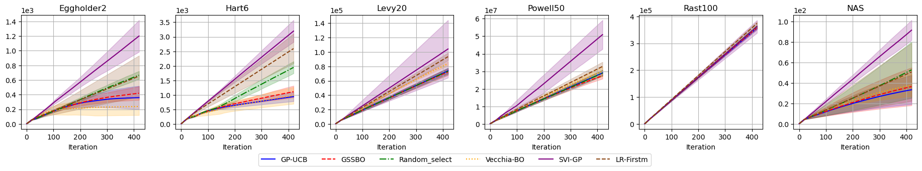
Figure 2: Cumulative regret of algorithms on the Eggholder2, Hart6, Levy20, Powell50, Rastrigin100 functions and NAS experiment.

In this section, we conduct numerical experiments to illustrate the superior efficiency of GSSBO. The objective of the numerical experiments are threefold: (1) to evaluate computational efficiency; (2) to assess optimization performance; and (3) to validate the theoretical analysis.

Experimental Setup.

We choose UCB as the acquisition function in GSSBO, and compare GSSBO with the following benchmarks: (1) Standard GP-UCB (Srinivas et al., 2009), which retains all observed samples without any selection; (2) Random Sample Selection GP-UCB (RSSBO), which mirrors our approach in restricting the sample set size but chooses which samples to keep purely at random; (3) VecchiaBO (Jimenez & Katzfuss, 2023), which utilizes the Vecchia approximation method to condition the GP likelihood on the nearest neighbors in a predefined maximization order; (4) SVIGP (Hensman et al., 2013), which applies stochastic variational inference by optimizing pseudo-points to approximate the GP posterior; and (5) LR-First m (Williams & Seeger, 2000), which uses a low-rank approximation based on the first $m$ samples in a maximization order, with the conditioning set fixed across all samples. We employ a Matérn $5/2$ kernel for the GP, with hyperparameters learned via maximum likelihood estimation. Both GSSBO and RSSBO use the same buffer size $M$, dynamically adjusted by a parameter $Z=4$. The gradient-perturbation noise is set to $\sigma^{2}=0.01$. Each experiment is repeated 50 times to rule out accidental variations, and the total budget is 400.

6.1 Synthetic Test Problems

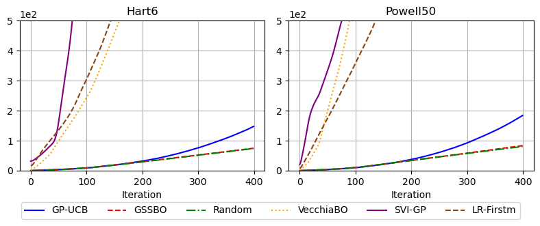
Figure 3: Cumulative time cost of algorithms (in seconds).

Figure 4: Sensitivity analysis of hyperparameter $Z$ on GSSBO.

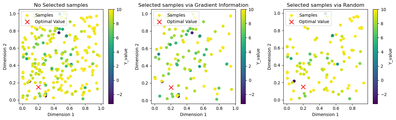
Figure 5: Sample distribution: no selection (left), gradient-based selection (middle), and random selection (right).

To assess the performance of our proposed methods, we test five benchmark functions, Eggholder2, Hart6, Levy20, Powell50, and Rastrigin100.

Computational Efficiency Analysis. Figure 3 compares the cumulative runtime over $400$ iterations on low-dimensional Hart6 and high-dimensional Powell50 (results for other test functions are provided in the appendix due to space constraints). In both plots, VecchiaBO, SVI-GP, and LR-Firstm incur a rapidly accelerating runtime, whereas GSSBO and RSSBO remain notably lower than GP-UCB. While VecchiaBO reduces the cost of GP fitting by conditioning on nearest neighbors, its runtime is dominated by the costly maintenance of a structured neighbor graph, which scales poorly with dimensionality and sample size. SVI-GP introduces significant overhead from iterative optimization of pseudo-points and variational parameters via gradient descent, particularly in high dimensions. LR-Firstm, despite a fixed subset size $m$, incurs substantial costs from repeated maximization ordering and matrix factorizations as $n$ grows. These methods aim to reduce the computational complexity of GPs in the context of large budgets, but they overlook the substantial time costs associated with their approximation processes. In contrast, GSSBO and RSSBO cost much less time. Because we use a pilot-based method to compute gradients with minimal computational overhead, the fitting cost per iteration of GSSBO remains around $\mathcal{O}(M^{3})$ once we restrict the active subset to size $M\ll n$. The GSSBO and the random one are often similar in runtime, though the GSSBO can be slightly higher due to the overhead of the gradient-based sample selection process. By iteration 400, the GSSBO cuts the total runtime by roughly half compared to the Standard GP-UCB on both functions. This advantage of GSSBO increases more pronounced as $n$ increases.

Optimization Performance Analysis. Figure 2 compares methods on multiple functions, evaluating cumulative regret. Overall, GSSBO achieves comparable performance with the Standard GP-UCB while outperforming the RSSBO. In low-dimensional problems such as Eggholder2 and Hart6, GSSBO has a subtle gap with Standard GP-UCB and VecchiaBO. In contrast, GSSBO significantly outperforms SVI-GP, LR-Firstm, and RSSBO. In high-dimensional settings, such as on Levy20, Powell50, and Rastrigin100, GSSBO achieves the smallest cumulative regret, surpassing VecchiaBO, SVI-GP and LR-Firstm. From the experimental results, we can observe that the cumulative of our algorithm is sublinear, which is consistent with the theoretical results. In particular, GSSBO achieves these results with a significant reduction in computation time, as shown in Figure 3. GSSBO strikes a combination of performance and efficiency in scalable optimization tasks by maintaining near-baseline regret while significantly improving computational efficiency.

Sensitivity analysis of Hyperparameter $Z$. We further examine how the dynamic buffer parameter $Z$ affects our GSSBO. Figure 4 presents results on two functions: Hart6 and Powell50. For RSSBO, $Z$ remains fixed at 4, whereas for GSSBO, we vary $Z\in\{2,4,6,8\}$. On Hart6, larger $Z$ consistently boosts the GSSBO’s performance toward that of Standard GP-UCB, while the RSSBO lags in cumulative regret. Intuitively, for low dimensional problems, allowing the model to retain more samples helps preserve important information, bridging the gap with the Standard GP-UCB baseline. In contrast, in Powell50, smaller $Z$ leads to slightly better performances for GSSBO, reflecting the benefit of subset updates in high-dimensional landscapes. Sample selection maintains a robust exploration-exploitation balance. In general, low-dimensional tasks benefit from a larger $Z$, while high-dimensional problems perform better with more aggressive subset limiting, $Z$ can be effectively tuned to match the complexity of tasks.

6.2 Real-World Application

To assess the applicability of GSSBO in real-world applications, we applied Neural Architecture Search (NAS) to a diabetes-detection problem and used the diabetes dataset from the UCI repository (Dua & Graff, 2017). We modeled the problem of searching for optimal hyperparameters as a BO problem. Specifically, each query $(x_{t},y_{t})$ corresponds to a choice of (batch size, Learning Rate, Learning Rate decay, hidden dim) in $[0,1]^{4}$ mapped to real hyperparameter ranges, where $y_{t}$ is the resulting classification error on the test set. Each iteration is repeated 5 times. The results in Figure 2 indicate that GSSBO outperforms all competitors.

6.3 Subset Samples Distribution Study

Figure 5 illustrates the sample distribution of GSSBO and Standard GP-UCB, on the first two dimensions of the Hartmann6 function. In this experiment, we recorded the first 200 sequential samples from a standard BO process and constrained the buffer size to 100. The objective is to identify the global minimum, and darker-colored samples correspond to values closer to the optimal solution.

During the optimization process, only a small number of samples are located near the optimal value (represented as the darker-colored samples being sparse). As shown in the middle panel, the gradient-based sample selection method selects a more informative and diverse subset, retaining more samples closer to the optimal or suboptimal, which is indicated by preserving a higher number of darker-colored samples in the figure. In contrast, the random selection strategy reduces the sample density uniformly across all regions, leading to a significant loss of samples near the optimal or suboptimal, as represented by the retention of many lighter-colored samples in the right panel. With gradient-based sample selection, the relative density of samples near the optimal and suboptimal regions increases, maintaining a more balanced distribution. This subset encourages subsequent iterations to focus on regions outside the optimal and suboptimal regions, promoting the exploration of other regions of the search space. As a result, the over-exploitation issue is mitigated.

7 Conclusion

BO is known to be effective for optimization in settings where the objective function is expensive to evaluate. In large-budget scenarios, the use of a full GP model can slow the convergence of BO, leading to poor scaling in these cases. In this paper, we investigated the use of gradient-based sample selection to accelerate BO, demonstrating how a carefully constructed subset, guided by gradient information, can serve as an efficient surrogate for the full sample set, significantly enhancing the efficiency of the BO process. As we have shown in a comprehensive set of experiments, the proposed GSSBO shows its ability to significantly reduce computational time while maintaining competitive optimization performance. Synthetic benchmarks highlight its scalability across various problem dimensions, while real-world applications confirm its practical utility. The sensitivity analysis further showcases the adaptability of the method to different parameter settings, reinforcing its robustness in diverse optimization scenarios. Overall, these findings underline the potential of gradient-based sample selection in addressing the scaling challenges of BO.

Appendix A Theoretical Analysis

A.1 Theorem 1:Analysis on subset GP:

Consider a GP model, where we assume $f(\mathbf{x})\sim\mathcal{GP}(0,k(\mathbf{x},\mathbf{x}^{\prime})),$ and given samples $\mathcal{D}=\{(\mathbf{x}_{1},y_{1}),\ldots,(\mathbf{x}_{t},y_{t})\}$, where $\mathbf{x}_{i}\in\mathbb{R}^{d}$ and $y_{i}\in\mathbb{R}$, we have a noise model: $\mathbf{y}=f(\mathbf{X})+\bm{\epsilon},\quad\bm{\epsilon}\sim\mathcal{N}(0,\sigma_{n}^{2}\mathbf{I}),$ where $\mathbf{X}=[\mathbf{x}_{1},\mathbf{x}_{2},\ldots,\mathbf{x}_{t}]^{\top}\in\mathbb{R}^{t\times d}$ and $\mathbf{y}=[y_{1},y_{2},\ldots,y_{t}]^{\top}\in\mathbb{R}^{t}$. The posterior predictive distribution for a test point $\mathbf{x}_{*}$ is Gaussian with the following mean and variance: $\mu(\mathbf{x}_{*})=\mathbf{k}_{*}^{\top}(\mathbf{K}+\sigma_{n}^{2}\mathbf{I})^{-1}\mathbf{y},$ $\sigma^{2}(\mathbf{x}_{*})=k_{**}-\mathbf{k}_{*}^{\top}(\mathbf{K}+\sigma_{n}^{2}\mathbf{I})^{-1}\mathbf{k}_{*},$ where $\mathbf{K}$ is the $t\times t$ kernel matrix evaluated at the training samples, i.e., $\mathbf{K}_{ij}=k(\mathbf{x}_{i},\mathbf{x}_{j})$; $\mathbf{k}_{*}\in\mathbb{R}^{t}$ is the vector of covariances between the test point $\mathbf{x}_{*}$ and all training points, i.e., $(\mathbf{k}_{*})_{i}=k(\mathbf{x}_{*},\mathbf{x}_{i})$; $k_{**}=k(\mathbf{x}_{*},\mathbf{x}_{*})$ is the kernel evaluated at the test point itself.

Sparse Approximation Using a Subset of Samples

Instead of using all $N$ training samples, consider a subset samples $\mathcal{U}=\{\mathbf{u}_{1},\dots,\mathbf{u}_{M}\}$, where $M\ll N$. Define: $\mathbf{K}_{\mathcal{U}\mathcal{U}}\in\mathbb{R}^{M\times M},\quad\mathbf{K}_{\mathcal{D}\mathcal{U}}\in\mathbb{R}^{N\times M},\quad\mathbf{K}_{\mathcal{U}\mathcal{D}}=\mathbf{K}_{\mathcal{D}\mathcal{U}}^{\top},$ where $\mathbf{K}_{\mathcal{U}\mathcal{U}}$ is the kernel matrix among the $M$ inducing points, and $\mathbf{K}_{\mathcal{D}\mathcal{U}}$ represents the covariances between the full training samples in $\mathcal{D}$ and the inducing points in $\mathcal{U}$. Using Subset of Regressors (SoR), a low-rank approximation to the kernel matrix $\mathbf{K}_{\mathcal{D}\mathcal{D}}\in\mathbb{R}^{N\times N}$ is given by: $\hat{\mathbf{K}}=\mathbf{K}_{\mathcal{D}\mathcal{U}}\mathbf{K}_{\mathcal{U}\mathcal{U}}^{-1}\mathbf{K}_{\mathcal{U}\mathcal{D}}.$ We can get the corresponding approximate posterior predictive mean using matrix decomposition and Woodbury formula for transformation.

Replacing $\mathbf{K}_{\mathcal{D}\mathcal{D}}$ with $\hat{\mathbf{K}}$, the posterior predictive mean becomes: $\mu(\mathbf{x}_{*})=\mathbf{k}_{*}^{\top}\left(\mathbf{K}_{\mathcal{D}\mathcal{U}}\mathbf{K}_{\mathcal{U}\mathcal{U}}^{-1}\mathbf{K}_{\mathcal{U}\mathcal{D}}+\sigma_{n}^{2}\mathbf{I}\right)^{-1}\mathbf{y}.$ The Woodbury matrix formula states: $(\mathbf{U}\mathbf{V}+\mathbf{C})^{-1}=\mathbf{C}^{-1}-\mathbf{C}^{-1}\mathbf{U}(\mathbf{V}^{-1}+\mathbf{U}^{\top}\mathbf{C}^{-1}\mathbf{U})^{-1}\mathbf{U}^{\top}\mathbf{C}^{-1}.$ In our case: $\mathbf{C}=\sigma_{n}^{2}\mathbf{I}\in\mathbb{R}^{N\times N}$, $\mathbf{U}=\mathbf{K}_{\mathcal{D}\mathcal{U}}\in\mathbb{R}^{N\times M}$, $\mathbf{V}=\mathbf{K}_{\mathcal{U}\mathcal{U}}^{-1}\in\mathbb{R}^{M\times M}$. We have: $\left(\mathbf{K}_{\mathcal{D}\mathcal{U}}\mathbf{K}_{\mathcal{U}\mathcal{U}}^{-1}\mathbf{K}_{\mathcal{U}\mathcal{D}}+\sigma_{n}^{2}\mathbf{I}\right)^{-1}=\sigma_{n}^{-2}\mathbf{I}-\sigma_{n}^{-4}\mathbf{K}_{\mathcal{D}\mathcal{U}}\left(\mathbf{K}_{\mathcal{U}\mathcal{U}}+\sigma_{n}^{2}\mathbf{I}\right)^{-1}\mathbf{K}_{\mathcal{U}\mathcal{D}}.$ Substituting this result back into the posterior predictive mean:

$$\tilde{\mu}(\mathbf{x}_{*})=\mathbf{k}_{*}^{\top}\left[\sigma_{n}^{-2}\mathbf{I}-\sigma_{n}^{-4}\mathbf{K}_{\mathcal{D}\mathcal{U}}\left(\mathbf{K}_{\mathcal{U}\mathcal{U}}+\sigma_{n}^{2}\mathbf{I}\right)^{-1}\mathbf{K}_{\mathcal{U}\mathcal{D}}\right]\mathbf{y}$$

$$=\sigma_{n}^{-2}\mathbf{k}_{*}^{\top}\mathbf{y}-\mathbf{k}_{*}^{\top}\sigma_{n}^{-4}\mathbf{K}_{\mathcal{D}\mathcal{U}}\left(\mathbf{K}_{\mathcal{U}\mathcal{U}}+\sigma_{n}^{2}\mathbf{I}\right)^{-1}\mathbf{K}_{\mathcal{U}\mathcal{D}}\mathbf{y}$$

$$=\sigma_{n}^{-2}\mathbf{k}_{*}^{\top}\mathbf{y}-\sigma_{n}^{-4}\mathbf{k}_{*\mathcal{U}}^{\top}\left(\mathbf{K}_{\mathcal{U}\mathcal{U}}+\sigma_{n}^{2}\mathbf{I}\right)^{-1}\mathbf{K}_{\mathcal{U}\mathcal{D}}\mathbf{y}$$

$$=\mathbf{k}_{*\mathcal{U}}^{\top}(\mathbf{K}_{\mathcal{U}\mathcal{U}}+\sigma_{n}^{2}\mathbf{I})^{-1}\mathbf{K}_{\mathcal{U}\mathcal{D}}\mathbf{y}.$$

where $\mathbf{k}_{*\mathcal{U}}=\mathbf{k}_{*}^{\top}\mathbf{K}_{\mathcal{D}\mathcal{U}}$ represents the covariance vector between the test point $\mathbf{x}_{*}$ and the $M$ inducing samples.

In addition to the predictive mean, the exact posterior predictive variance of a GP is given by: $\sigma^{2}(\mathbf{x}_{*})=k_{**}-\mathbf{k}_{*}^{\top}(\mathbf{K}_{\mathcal{D}\mathcal{D}}+\sigma_{n}^{2}\mathbf{I})^{-1}\mathbf{k}_{*},$ where $k_{**}=k(\mathbf{x}_{*},\mathbf{x}_{*})$ is the kernel evaluated at the test point. Under the sparse approximation (SoR), the approximate posterior predictive variance is:

$$\tilde{\sigma}^{2}(\mathbf{x}_{*})=k_{**}-\mathbf{k}_{*\mathcal{U}}^{\top}(\mathbf{K}_{\mathcal{U}\mathcal{U}}+\sigma_{n}^{2}\mathbf{I})^{-1}\mathbf{k}_{\mathcal{U}*},$$

where $\mathbf{k}_{*\mathcal{U}}$ is the vector of covariances between the test point $\mathbf{x}_{*}$ and the $M$ inducing points, and $\mathbf{k}_{\mathcal{U}*}=\mathbf{k}_{*\mathcal{U}}^{\top}$.

Error Characterization by Kernel Approximation and Variance Error Analysis

We aim to bound the difference between the exact posterior distribution and the approximate posterior distribution. The differences in the posterior predictive mean and variance can be expressed as: $\Delta\mu(\mathbf{x}_{*})=\mu(\mathbf{x}_{*})-\tilde{\mu}(\mathbf{x}_{*}),$ $\Delta\sigma^{2}(\mathbf{x}_{*})=\sigma^{2}(\mathbf{x}_{*})-\tilde{\sigma}^{2}(\mathbf{x}_{*}).$ Starting with the mean difference, the exact posterior predictive mean and the approximate mean are given by: $\mu(\mathbf{x}_{*})=\mathbf{k}_{*\mathcal{D}}^{\top}(\mathbf{K}_{\mathcal{D}\mathcal{D}}+\sigma_{n}^{2}\mathbf{I})^{-1}\mathbf{y},$ $\tilde{\mu}(\mathbf{x}_{*})=\mathbf{k}_{*\mathcal{D}}^{\top}(\hat{\mathbf{K}}+\sigma_{n}^{2}\mathbf{I})^{-1}\mathbf{y}.$ Thus, the mean difference becomes:

$$\Delta\mu(\mathbf{x}_{*})=\mathbf{k}_{*\mathcal{D}}^{\top}\left[(\mathbf{K}_{\mathcal{D}\mathcal{D}}+\sigma_{n}^{2}\mathbf{I})^{-1}-(\hat{\mathbf{K}}+\sigma_{n}^{2}\mathbf{I})^{-1}\right]\mathbf{y}.$$

Define the following positive definite matrices: $\mathbf{A}=\mathbf{K}_{\mathcal{D}\mathcal{D}}+\sigma_{n}^{2}\mathbf{I},\quad\mathbf{B}=\hat{\mathbf{K}}+\sigma_{n}^{2}\mathbf{I}.$ Then, the difference between $\mathbf{A}$ and $\mathbf{B}$ is: $\mathbf{A}-\mathbf{B}=\mathbf{K}_{\mathcal{D}\mathcal{D}}-\hat{\mathbf{K}}.$ We have $\|A^{-1}-B^{-1}\|\;\;\leq\;\;\|A^{-1}\|\,\|B^{-1}\|\;\|A-B\|,$ and take $C_{1}\;=\;\|A^{-1}\|\;\|B^{-1}\|.$ $A,B$ are positive definite, denote $\lambda_{\min}(A)\;=\;\text{the smallest eigenvalue of }A,\quad\lambda_{\min}(B)\;=\;\text{the smallest eigenvalue of }B.$ Then $\|A^{-1}\|\;=\;\frac{1}{\lambda_{\min}(A)},\quad\|B^{-1}\|\;=\;\frac{1}{\lambda_{\min}(B)},$ when the norm is the usual spectral/operator norm. Hence, $C_{1}\;=\;\|A^{-1}\|\;\|B^{-1}\|\;\;\leq\;\frac{1}{\lambda_{\min}(A)\,\lambda_{\min}(B)}.$ We have: $\|(\mathbf{K}_{\mathcal{D}\mathcal{D}}+\sigma_{n}^{2}\mathbf{I})^{-1}-(\hat{\mathbf{K}}+\sigma_{n}^{2}\mathbf{I})^{-1}\|\leq C_{1}\|\mathbf{K}_{\mathcal{D}\mathcal{D}}-\hat{\mathbf{K}}\|.$ Substituting this into the expression for $\Delta\mu(\mathbf{x}_{*})$, we obtain:

$$|\Delta\mu(\mathbf{x}_{*})|\leq\|\mathbf{k}_{*\mathcal{D}}\|\|\mathbf{y}\|\|(\mathbf{K}_{\mathcal{D}\mathcal{D}}+\sigma_{n}^{2}\mathbf{I})^{-1}-(\hat{\mathbf{K}}+\sigma_{n}^{2}\mathbf{I})^{-1}\|$$

$$\leq\|\mathbf{k}_{*\mathcal{D}}\|\|\mathbf{y}\|C_{1}\|\mathbf{K}_{\mathcal{D}\mathcal{D}}-\hat{\mathbf{K}}\|.$$

The approximate posterior predictive variance is given by: $\tilde{\sigma}^{2}(\mathbf{x}_{*})=k_{**}-\mathbf{k}_{*\mathcal{D}}^{\top}(\hat{\mathbf{K}}+\sigma_{n}^{2}\mathbf{I})^{-1}\mathbf{k}_{*\mathcal{D}},$ where $\hat{\mathbf{K}}=\mathbf{K}_{\mathcal{D}\mathcal{U}}\mathbf{K}_{\mathcal{U}\mathcal{U}}^{-1}\mathbf{K}_{\mathcal{U}\mathcal{D}}$ is the low-rank approximation to $\mathbf{K}_{\mathcal{D}\mathcal{D}}$. Define the variance error as: $\Delta\sigma^{2}(\mathbf{x}_{*})=\sigma^{2}(\mathbf{x}_{*})-\tilde{\sigma}^{2}(\mathbf{x}_{*}).$ The variance error can be expressed as:

$$\Delta\sigma^{2}(\mathbf{x}_{*})=\left[k_{**}-\mathbf{k}_{*\mathcal{D}}^{\top}(\mathbf{K}_{\mathcal{D}\mathcal{D}}+\sigma_{n}^{2}\mathbf{I})^{-1}\mathbf{k}_{*\mathcal{D}}\right]-\left[k_{**}-\mathbf{k}_{*\mathcal{D}}^{\top}(\hat{\mathbf{K}}+\sigma_{n}^{2}\mathbf{I})^{-1}\mathbf{k}_{*\mathcal{D}}\right].$$

$$=\mathbf{k}_{*\mathcal{D}}^{\top}\left[(\hat{\mathbf{K}}+\sigma_{n}^{2}\mathbf{I})^{-1}-(\mathbf{K}_{\mathcal{D}\mathcal{D}}+\sigma_{n}^{2}\mathbf{I})^{-1}\right]\mathbf{k}_{*\mathcal{D}}.$$

From the mean error analysis, we know: $\|(\mathbf{K}_{\mathcal{D}\mathcal{D}}+\sigma_{n}^{2}\mathbf{I})^{-1}-(\hat{\mathbf{K}}+\sigma_{n}^{2}\mathbf{I})^{-1}\|\leq C_{1}\|\mathbf{K}_{\mathcal{D}\mathcal{D}}-\hat{\mathbf{K}}\|,$ for some constant $C_{1}$ that depends on the spectral properties of the matrices. Using the spectral norm (or any subordinate matrix norm), the variance error can be bounded as: $|\Delta\sigma^{2}(\mathbf{x}_{*})|=\left|\mathbf{k}_{*\mathcal{D}}^{\top}\left[(\hat{\mathbf{K}}+\sigma_{n}^{2}\mathbf{I})^{-1}-(\mathbf{K}_{\mathcal{D}\mathcal{D}}+\sigma_{n}^{2}\mathbf{I})^{-1}\right]\mathbf{k}_{*\mathcal{D}}\right|.$ Applying the properties of matrix norms and the Cauchy–Schwarz inequality:

$$|\Delta\sigma^{2}(\mathbf{x}_{*})|\leq\|\mathbf{k}_{*\mathcal{D}}\|^{2}\|(\hat{\mathbf{K}}+\sigma_{n}^{2}\mathbf{I})^{-1}-(\mathbf{K}_{\mathcal{D}\mathcal{D}}+\sigma_{n}^{2}\mathbf{I})^{-1}\|.$$

$$\leq\|\mathbf{k}_{*\mathcal{D}}\|^{2}C_{1}\|\mathbf{K}_{\mathcal{D}\mathcal{D}}-\hat{\mathbf{K}}\|.$$

Impact of the “Maximum Gradient Variance” Principle in Selecting Subsamples

The “Maximum Gradient Variance” principle for selecting the inducing points (or subsample set) aims to pick points that best capture the main gradient variations in the sample distribution, ensuring that $\mathbf{K}_{\mathcal{D}\mathcal{D}}\approx\hat{\mathbf{K}}$ accurately. As $M$ increases and the subset points are chosen more effectively, the approximation $\hat{\mathbf{K}}$ to $\mathbf{K}_{\mathcal{D}\mathcal{D}}$ improves, hence $\|\mathbf{K}_{\mathcal{D}\mathcal{D}}-\hat{\mathbf{K}}\|$ decreases. Consider a set of $N$ samples $\mathcal{D}=\{\mathbf{x}_{1},\dots,\mathbf{x}_{N}\}$ and a corresponding kernel matrix: $\mathbf{K}_{\mathcal{D}\mathcal{D}}\in\mathbb{R}^{N\times N},\quad(\mathbf{K}_{\mathcal{D}\mathcal{D}})_{ij}=k(\mathbf{x}_{i},\mathbf{x}_{j}),$ where $k$ is a positive definite kernel. Suppose we have observations $\mathbf{y}\in\mathbb{R}^{N}$ associated with these samples, and a probabilistic model (e.g., a GP) with parameters ${\theta}$ and the mean function $\mu$. The joint distribution of $\mathbf{y}$ given $\mathcal{D}$ and ${\theta}$ is: $\mathbf{y}\mid\mathcal{D},{\theta}\sim\mathcal{N}(\mu,\mathbf{K}_{\mathcal{D}\mathcal{D}}),$ where $\mathbf{K}_{\mathcal{D}\mathcal{D}}$ is the covariance matrix induced by the kernel $k$. Define the gradient of the log-posterior (or log-likelihood) with respect to the latent function values $\mathbf{y}$: $g_{i}=\frac{\partial\log p(\mathbf{y}\mid\mathcal{D},{\theta})}{\partial y_{i}}=-(\mathbf{K}_{\mathcal{D}\mathcal{D}}^{-1}(\mathbf{y}-\mu))_{i}.$

Now we force the initial batch of $n_{0}$ samples $\{\mathbf{x}_{1},\dots,\mathbf{x}_{n_{0}}\}$ and the latest sample $\mathbf{x}_{\mathrm{L}}$ to be included in $\mathcal{U}$. We then choose the remaining $M-n_{0}-1$ samples to maximize gradient variance. We select the $M-n_{0}-1$ samples that maximize the variance of gradient information. We have $\mathcal{U}\;=\;\{\mathbf{x}_{1},\dots,\mathbf{x}_{n_{0}}\}\;\cup\;\{\mathbf{x}_{\mathrm{L}}\}\;\cup\;\mathcal{U}^{\prime},$ where $|\mathcal{U}^{\prime}|=M-n_{0}-1$ so that $|\mathcal{U}|=M$, the total subset $\mathcal{U}$ is still of size $M$. We consider a subset $\mathcal{U}\subset\mathcal{D}$ of size $M<N$ to build a low-rank approximation of $\mathbf{K}_{\mathcal{D}\mathcal{D}}$: $\hat{\mathbf{K}}=\mathbf{K}_{\mathcal{D}\mathcal{U}}\mathbf{K}_{\mathcal{U}\mathcal{U}}^{-1}\mathbf{K}_{\mathcal{U}\mathcal{D}},$ where $\mathbf{K}_{\mathcal{U}\mathcal{U}}$ and $\mathbf{K}_{\mathcal{D}\mathcal{U}}$ are derived from $\mathcal{U}$. Let $\mathcal{D}=\{\mathbf{x}_{1},\dots,\mathbf{x}_{N}\}$ and $\mathbf{K}_{\mathcal{D}\mathcal{D}}\in\mathbb{R}^{N\times N}$ be a positive definite kernel matrix with eigen-decomposition: $\mathbf{K}_{\mathcal{D}\mathcal{D}}=\mathbf{U}\bm{\Lambda}\mathbf{U}^{\top},$ where $\bm{\Lambda}=\mathrm{diag}(\lambda_{1},\ldots,\lambda_{N})$ with $\lambda_{1}\geq\lambda_{2}\geq\cdots\geq\lambda_{N}\geq 0$ and $\mathbf{U}=[\mathbf{u}_{1},\ldots,\mathbf{u}_{N}]$. The best rank-$M$ approximation to $\mathbf{K}_{\mathcal{D}\mathcal{D}}$ in spectral norm is: $\mathbf{K}_{\mathcal{D}\mathcal{D}}^{(M)}=\mathbf{U}_{M}\bm{\Lambda}_{M}\mathbf{U}_{M}^{\top},$ where $\mathbf{U}_{M}=[\mathbf{u}_{1},\dots,\mathbf{u}_{M}]$ and $\bm{\Lambda}_{M}=\mathrm{diag}(\lambda_{1},\dots,\lambda_{M})$. By the Eckart–Young–Mirsky theorem: $\|\mathbf{K}_{\mathcal{D}\mathcal{D}}-\mathbf{K}_{\mathcal{D}\mathcal{D}}^{(M)}\|=\lambda_{M+1}.$ Suppose $\mathcal{U}\subset\mathcal{D}$, $|\mathcal{U}|=M$, produces a Nyström approximation: $\hat{\mathbf{K}}=\mathbf{K}_{\mathcal{D}\mathcal{U}}\mathbf{K}_{\mathcal{U}\mathcal{U}}^{-1}\mathbf{K}_{\mathcal{U}\mathcal{D}}.$ If the subset $\mathcal{U}$ is chosen to approximate the principal eigenspace spanned by $\mathbf{U}_{M}$, then Nyström approximation theory (Drineas et al., 2005) guarantees that: $\|\mathbf{K}_{\mathcal{D}\mathcal{D}}-\hat{\mathbf{K}}\|\leq\|\mathbf{K}_{\mathcal{D}\mathcal{D}}-\mathbf{K}_{\mathcal{D}\mathcal{D}}^{(M)}\|+\epsilon\sum_{i=1}^{N}(\mathbf{K}_{\mathcal{D}\mathcal{D}})_{ii}^{2}=\lambda_{M+1}+\epsilon\sum_{i=1}^{N}(\mathbf{K}_{\mathcal{D}\mathcal{D}})_{ii}^{2}.$ where $\epsilon$ is an error control parameter related to the number of columns sampled randomly in the approximation.

Error Bound for UCB under Sparse GP Approximation

Let the UCB for the full GP model be defined as: $\mathrm{UCB}(\mathbf{x}_{*})=\mu(\mathbf{x}_{*})+\beta\sigma(\mathbf{x}_{*}),$ where $\mu(\mathbf{x}_{*})$ and $\sigma(\mathbf{x}_{*})$ are the posterior predictive mean and standard deviation under the full GP, respectively. For the sparse GP approximation, the UCB is given by: $\tilde{\mathrm{UCB}}(\mathbf{x}_{*})=\tilde{\mu}(\mathbf{x}_{*})+\beta\tilde{\sigma}(\mathbf{x}_{*}),$ where $\tilde{\mu}(\mathbf{x}_{*})$ and $\tilde{\sigma}(\mathbf{x}_{*})$ are the posterior predictive mean and standard deviation under the sparse GP approximation.

We aim to bound the error:

$$|\mathrm{UCB}(\mathbf{x}_{*})-\tilde{\mathrm{UCB}}(\mathbf{x}_{*})|,$$

in terms of the kernel matrix approximation error $\|\mathbf{K}_{\mathcal{D}\mathcal{D}}-\hat{\mathbf{K}}\|$. Given the bounds:

$$|\Delta\mu(\mathbf{x}_{*})|\leq\|\mathbf{k}_{*\mathcal{D}}\|\|\mathbf{y}\|C_{1}\|\mathbf{K}_{\mathcal{D}\mathcal{D}}-\hat{\mathbf{K}}\|,$$

$$|\Delta\sigma(\mathbf{x}_{*})|\leq\|\mathbf{k}_{*\mathcal{D}}\|\sqrt{C_{1}\|\mathbf{K}_{\mathcal{D}\mathcal{D}}-\hat{\mathbf{K}}\|}.$$

The error of UCB in one iteration can be expressed as:

$$\bigl{|}\mathrm{UCB}(\mathbf{x}_{*})-\tilde{\mathrm{UCB}}(\mathbf{x}_{*})\bigr{|}\;=\;\bigl{|}\Delta\mu(\mathbf{x}_{*})+\beta\,\Delta\sigma(\mathbf{x}_{*})\bigr{|}\;\;\leq\;\;\bigl{|}\Delta\mu(\mathbf{x}_{*})\bigr{|}\;+\;\beta\,\bigl{|}\Delta\sigma(\mathbf{x}_{*})\bigr{|}.$$

Substituting the bounds for $|\Delta\mu(\mathbf{x}_{*})|$ and $|\Delta\sigma(\mathbf{x}_{*})|$, we have:

$$|\mathrm{UCB}(\mathbf{x}_{*})-\tilde{\mathrm{UCB}}(\mathbf{x}_{*})|\leq\|\mathbf{k}_{*\mathcal{D}}\|\|\mathbf{y}\|C_{1}\|\mathbf{K}_{\mathcal{D}\mathcal{D}}-\hat{\mathbf{K}}\|+\beta\|\mathbf{k}_{*\mathcal{D}}\|\sqrt{C_{1}\|\mathbf{K}_{\mathcal{D}\mathcal{D}}-\hat{\mathbf{K}}\|}.$$

Using the Nyström approximation error bound $\|\mathbf{K}_{\mathcal{D}\mathcal{D}}-\hat{\mathbf{K}}\|\leq C^{\prime}\lambda_{M+1}$, the UCB error can be further bounded as:

$$|\mathrm{UCB}(\mathbf{x}_{*})-\tilde{\mathrm{UCB}}(\mathbf{x}_{*})|\leq\|\mathbf{k}_{*\mathcal{D}}\|\|\mathbf{y}\|C_{1}(\lambda_{M+1}+\epsilon\sum_{i=1}^{N}(\mathbf{K}_{\mathcal{D}\mathcal{D}})_{ii}^{2})+\beta\|\mathbf{k}_{*\mathcal{D}}\|\sqrt{C_{1}(\lambda_{M+1}+\epsilon\sum_{i=1}^{N}(\mathbf{K}_{\mathcal{D}\mathcal{D}})_{ii}^{2})}.$$

Merging Linear and $\beta$-Proportional Terms into a Single Penalty

We consider a GP scenario where the full GP-UCB at a point $\mathbf{x}$ is given by $\mathrm{UCB}(\mathbf{x})\;=\;\mu(\mathbf{x})\;+\;\beta\,\sigma(\mathbf{x}),$ while its approximate (or sparse) counterpart is $\tilde{\mathrm{UCB}}(\mathbf{x})\;=\;\tilde{\mu}(\mathbf{x})\;+\;\beta\,\tilde{\sigma}(\mathbf{x}).$ We have established the following pointwise error bound:

$$\bigl{|}\mathrm{UCB}(\mathbf{x})-\tilde{\mathrm{UCB}}(\mathbf{x})\bigr{|}\;\;\leq\;\;\underbrace{\|\mathbf{k}_{*\mathcal{D}}\|\|\mathbf{y}\|\;C_{1}\,(\lambda_{M+1}+\epsilon\sum_{i=1}^{N}(\mathbf{K}_{\mathcal{D}\mathcal{D}})_{ii}^{2}))}_{\displaystyle A}\;+\;\underbrace{\beta\,\|\mathbf{k}_{*\mathcal{D}}\|\sqrt{C_{1}\,(\lambda_{M+1}+\epsilon\sum_{i=1}^{N}(\mathbf{K}_{\mathcal{D}\mathcal{D}})_{ii}^{2})}}_{\displaystyle\beta B}.$$

Hence we obtain the typical form $A=O(\lambda_{M+1}),\quad B=O\bigl{(}\sqrt{\lambda_{M+1}}\bigr{)},$ and $\bigl{|}\mathrm{UCB}(\mathbf{x})-\tilde{\mathrm{UCB}}(\mathbf{x})\bigr{|}\;\leq\;A\;+\;\beta\,B.$

We state the theorem that allows merging the term $A+\beta B$ into a single factor $(\beta+\delta)\,\tilde{\sigma}(\mathbf{x})$, under a crucial assumption that $\tilde{\sigma}(\mathbf{x})$ is bounded away from zero.

Theorem A.1 (Single-Penalty Construction).

Let $A\geq 0$ and $B\geq 0$ be constants as above, and assume there exists a lower bound $\tilde{\sigma}(\mathbf{x})\geq\sigma_{\min}>0$ for all $\mathbf{x}$ in the domain. Then one can define $\tilde{\beta}\;=\;\beta\;+\;\delta,\quad\text{where}\quad\delta=\frac{A}{\sigma_{\min}},$ so that $A+\beta\,B\;\;\leq\;\;(\beta+\delta)\,\tilde{\sigma}(\mathbf{x}),$ and therefore $\bigl{|}\mathrm{UCB}(\mathbf{x})-\tilde{\mathrm{UCB}}(\mathbf{x})\bigr{|}\;\leq\;(\beta+\delta)\,\tilde{\sigma}(\mathbf{x}).$ Hence, one may write a unified approximate UCB of the form $\widehat{\mathrm{UCB}}(\mathbf{x})\;=\;\tilde{\mu}(\mathbf{x})\;+\;\tilde{\beta}\,\tilde{\sigma}(\mathbf{x}),$ with $\tilde{\beta}:=\beta+\delta$, thereby absorbing both $A$ and $\beta\,B$ into a single penalty term.

Proof.

Step 1: Inequality Setup. We need to ensure that $A+\beta\,B\;\;\leq\;\;(\beta+\delta)\,\tilde{\sigma}(\mathbf{x}),$ for all $\mathbf{x}$ in the domain. By hypothesis, $\tilde{\sigma}(\mathbf{x})\geq\sigma_{\min}$ for all $\mathbf{x}$, hence $(\beta+\delta)\,\tilde{\sigma}(\mathbf{x})\;\;\geq\;\;(\beta+\delta)\,\sigma_{\min}.$ Thus it suffices to impose $A+\beta\,B\;\;\leq\;\;(\beta+\delta)\,\sigma_{\min}.$ Observing that $\beta\,B\leq\beta\,B+A$, it is enough to ensure, individually: $A\;\;\leq\;\;\delta\,\sigma_{\min},\quad\beta\,B\;\;\leq\;\;\beta\,\sigma_{\min}.$ The first part is enforced by $\delta=A/\sigma_{\min}$. The second part can hold if $B\leq\sigma_{\min}$; otherwise, we can slightly adjust $\delta$ to cover that as well.

Step 2: Concluding the Single Penalty. Hence for all $\mathbf{x}$, $A+\beta\,B\;\leq\;\delta\,\sigma_{\min}\;+\;\beta\,\sigma_{\min}\;=\;(\beta+\delta)\,\sigma_{\min}\;\leq\;(\beta+\delta)\,\tilde{\sigma}(\mathbf{x}).$ Therefore, $\bigl{|}\mathrm{UCB}(\mathbf{x})-\tilde{\mathrm{UCB}}(\mathbf{x})\bigr{|}\;\leq\;A+\beta\,B\;\leq\;(\beta+\delta)\,\tilde{\sigma}(\mathbf{x}).$ Defining $\tilde{\beta}=\beta+\delta$ yields $\bigl{|}\mathrm{UCB}(\mathbf{x})-\tilde{\mathrm{UCB}}(\mathbf{x})\bigr{|}\;\leq\;\tilde{\beta}\,\tilde{\sigma}(\mathbf{x}),$ establishing the desired single-penalty inequality. ∎

Combining Theorem A.1 with our pointwise error bound, we see the following: (1) We have already obtained that $\bigl{|}\mathrm{UCB}(\mathbf{x})-\tilde{\mathrm{UCB}}(\mathbf{x})\bigr{|}\;\leq\;A+\beta B,$ where $A=\|\mathbf{k}_{*\mathcal{D}}\|\|\mathbf{y}\|\;C_{1}\,(\lambda_{M+1}+\epsilon\sum_{i=1}^{N}(\mathbf{K}_{\mathcal{D}\mathcal{D}})_{ii}^{2}))$ and $B=\|\mathbf{k}_{*\mathcal{D}}\|\sqrt{C_{1}\,(\lambda_{M+1}+\epsilon\sum_{i=1}^{N}(\mathbf{K}_{\mathcal{D}\mathcal{D}})_{ii}^{2})}.$ (2)If, in addition, $\tilde{\sigma}(\mathbf{x})\geq\sigma_{\min}>0$ (i.e. the approximate standard deviation does not vanish), one can pick $\delta\geq A/\sigma_{\min}$ so that $A+\beta\,B\;\leq\;(\beta+\delta)\,\sigma_{\min}\;\leq\;(\beta+\delta)\,\tilde{\sigma}(\mathbf{x}).$ Therefore, the entire error $A+\beta B$ can be encoded by just increasing $\beta$ to $\tilde{\beta}=\beta+\delta$. In practice, however, this tends to be overly conservative in regions where $\tilde{\sigma}(\mathbf{x})$ is large, since $(\beta+\delta)\,\tilde{\sigma}(\mathbf{x})$ might become significantly larger than $A+\beta B$.

In summary, beginning from the Nyström-based UCB error bound

$$\bigl{|}\mathrm{UCB}(\mathbf{x})-\tilde{\mathrm{UCB}}(\mathbf{x})\bigr{|}\;\leq\;A+\beta B\;\leq\;(\beta+\delta)\,\sigma_{\min}\;\leq\;(\beta+\delta)\,\tilde{\sigma}(\mathbf{x})\quad\bigl{(}A=O(\lambda_{M+1}),\,B=O(\sqrt{\lambda_{M+1}})\bigr{)},$$

we have shown that, provided $\tilde{\sigma}(\mathbf{x})\geq\sigma_{\min}>0$, one can inflate $\beta$ to $\beta+\delta$ so as to cover both the linear $A$ term and the $\beta B$ term.

UCB Formulation via a Single Multiplicative Penalty.

Having established that the term $A$ and the $\beta$-proportional term $\beta B$ can be merged under a single inflated parameter $\bigl{|}\mathrm{UCB}(\mathbf{x})-\tilde{\mathrm{UCB}}(\mathbf{x})\bigr{|}\;\leq\;A+\beta\,B,$ with constants $A=\|\mathbf{k}_{*\mathcal{D}}\|\|\mathbf{y}\|CC^{\prime}\lambda_{M+1}$ and $B=\beta\|\mathbf{k}_{*\mathcal{D}}\|\sqrt{CC^{\prime}\lambda_{M+1}}$ independent of $\beta$. Assume further that there is a lower bound $\sigma(\mathbf{x})\geq\sigma_{\min}>0$ for all $\mathbf{x}$, so the GP’s true standard deviation never becomes arbitrarily small. In that case, the linear term $A$ and the $\beta$-proportional term $\beta B$ can be combined into a single multiplier by inflating $\beta$ to $\tilde{\beta}\;=\;\beta\;+\;\delta,\quad\text{where}\quad\delta=\frac{A}{\sigma_{\min}}.$ Hence, $A+\beta\,B\;\;\leq\;\;(\beta+\delta)\,\sigma_{\min}\;\;\leq\;\;(\beta+\delta)\,\sigma(\mathbf{x}),$ so that $A+\beta B$ is covered by $(\beta+\delta)\,\sigma(\mathbf{x})$. Thus, in place of the usual $\mu(\mathbf{x})+\beta\,\sigma(\mathbf{x}),$ the new UCB can be written as

$$\tilde{\mathrm{UCB}}(\mathbf{x})\;=\;\mu(\mathbf{x})\;+\;\tilde{\beta}\,\sigma(\mathbf{x}),\quad\text{where}\quad\tilde{\beta}=\beta+\delta=\beta+\frac{A}{\sigma_{\min}},\quad B\leq\sigma_{\text{min}}.$$

A.2 Theorem 2:Analysis on Regret Bound:

GP-UCB is a popular algorithm for sequential decision-making problems. We propose an extension to GP-UCB by incorporating gradient-based sampling. In this section, we prove that the regret of the GP-UCB algorithm with gradient-based sampling is bounded. We show that by selecting the subset of samples with the highest variance, we can achieve a regret bound. This approach leverages the information gained from gradient-based sampling to provide a robust regret bound. To aid in the theoretical analysis, we make the following assumptions.

Assumption 1: Assume there exist constants $a$, $b$, and $L$ such that the kernel function $k(\mathbf{x},\mathbf{x}^{\prime})$ satisfies a Lipschitz continuity condition, providing confidence bounds on the derivatives of the GP sample paths $f$:

$$P\left(\sup_{\mathbf{x}\in\mathcal{X}}\left|\frac{\partial f}{\partial x_{j}}\right|>L\right)\leq ae^{-L^{2}/b^{2}}\quad\text{for }j=1,\ldots,p.$$

A typical example of such a kernel is the squared exponential kernel $k(\mathbf{x},\mathbf{x}^{\prime})=\sigma^{2}\exp\left(-\frac{\|\mathbf{x}-\mathbf{x}^{\prime}\|^{2}}{2l^{2}}\right)$, where $l$ is the length-scale parameter and $\sigma^{2}$ represents the noise variance. This condition aligns with standard assumptions in the regret analysis of BO, as detailed by Srinivas et al. (2010). We now present the main theorem on the cumulative regret bound for the GSSBO.

$$\tilde{\mathrm{UCB}}(\mathbf{x})\;=\;\mu(\mathbf{x})\;+\;(\beta+\frac{A}{\sigma_{\min}})\,\sigma(\mathbf{x}).$$

Theorem A.2.

Let $\mathcal{X}\subset[0,r]^{p}$ be compact and convex, $p\in\mathbb{N}$, $r>0$. Under Assumption 1, for any arbitrarily small $\delta\in(0,1)$, choose $\tilde{\beta_{n}}=2\log\frac{4\pi_{n}}{\delta}+2p\log\left(n^{2}brp\sqrt{\log\left(\frac{4pa}{\delta}\right)}\right),$i.e.,

$$\beta_{n}=2\log\frac{4\pi_{n}}{\delta}+2p\log\left(n^{2}brp\sqrt{\log\left(\frac{4pa}{\delta}\right)}\right)-\frac{A}{\sigma_{\min}},$$

where $\sum_{n\geq 1}\pi_{n}^{-1}=1,\quad\pi_{n}>0$. As $n\to\infty$, we obtain a regret bound of $\mathcal{O}^{*}(\sqrt{pN\gamma_{N}})$. Specifically, with $C^{\prime}=\frac{8}{\log(1+\sigma^{-2})},$ we have:

$$P\left(R_{N}\leq\sqrt{C^{\prime}N\beta_{N}\gamma_{N}}\right)\geq 1-\delta.$$

Lemma A.3.

For any arbitrarily small $\delta_{1}\in(0,1)$, choose $\tilde{\beta_{n}}=2\log\frac{\pi_{n}}{\delta_{1}}$, i.e., $\beta_{n}=2\log\frac{\pi_{n}}{\delta_{1}}-\frac{A}{\sigma_{\min}}$ , where $\sum_{n\geq 1}\pi_{n}^{-1}=1$, $\pi_{n}>0$, then we have

$$P\left(|f(\mathbf{x}_{n})-\mu_{n-1}(\mathbf{x}_{n})|\leq d\tilde{\beta_{n}}^{1/2}\sigma_{n-1}(\mathbf{x}_{n})\right)\geq 1-\delta$$

Proof.

Assuming we are at stage $n$, all past decisions $\mathbf{x}_{1:n-1}=\{\mathbf{x}_{1},\ldots,\mathbf{x}_{n-1}\}$ made after the initial design are deterministic given $\mathbf{y}_{1:n-1}=\{y_{1},\ldots,y_{n-1}\}$. For any $\mathbf{x}_{n}\in\mathbb{R}^{p}$, we have $f(\mathbf{x}_{n})\sim\mathcal{N}(\mu_{n-1}(\mathbf{x}_{n}),\sigma^{2}_{n-1}(\mathbf{x}_{n}))$.

For a standard normal variable $r\sim\mathcal{N}(0,1)$, the probability of being above a certain constant $c$ is written as:

$$P(r>c)=\frac{1}{\sqrt{2\pi}}\int_{c}^{\infty}e^{-r^{2}/2}\,dr$$

$$=e^{-c^{2}/2}\frac{1}{\sqrt{2\pi}}\int_{c}^{\infty}e^{-(r-c)^{2}/2-c(r-c)}\,dr$$

$$\leq e^{-c^{2}/2}\frac{1}{\sqrt{2\pi}}\int_{c}^{\infty}e^{-(r-c)^{2}/2}\,dr$$

$$=e^{-c^{2}/2}P(r>0)$$

$$=\frac{1}{2}e^{-c^{2}/2}$$

where the inequality holds due to the fact that $e^{-c(r-c)}\leq 1$ for $r\geq c>0$.

Plugging in $r=\frac{f(\mathbf{x}_{n})-\mu_{n-1}(\mathbf{x}_{n})}{\sigma_{n-1}(\mathbf{x}_{n})}$ and $c=\tilde{\beta_{n}}^{1/2}$, we have:

$$P\left(\left|f(\mathbf{x}_{n})-\mu_{n-1}(\mathbf{x}_{n})\right|>\tilde{\beta_{n}}^{1/2}\sigma_{n-1}(\mathbf{x}_{n})\right)\leq e^{-\frac{\tilde{\beta_{n}}}{2}}.$$

Equivalently,

$$P\left(\left|f(\mathbf{x}_{n})-\mu_{n-1}(\mathbf{x}_{n})\right|\leq\tilde{\beta_{n}}^{1/2}\sigma_{n-1}(\mathbf{x}_{n})\right)\geq 1-e^{-\frac{\tilde{\beta_{n}}}{2}}.$$

Choosing $e^{-\frac{\tilde{\beta_{n}}}{2}}=\frac{\delta}{\pi_{n}}$, i.e., $\tilde{\beta_{n}}=2\log\frac{\pi_{n}}{\delta}$, and applying the union bound for all possible values of stage $n$, we have:

$$P\left(\left|f(\mathbf{x}_{n})-\mu_{n-1}(\mathbf{x}_{n})\right|\leq\tilde{\beta_{n}}^{1/2}\sigma_{n-1}(\mathbf{x}_{n})\right)\geq 1-\sum_{n\geq 1}\frac{\delta}{\pi_{n}}=1-\delta.$$

where we have used the condition that $\sum_{n\geq 1}\pi_{n}^{-1}=1$, which can be obtained by setting $\pi_{n}=\frac{\pi^{2}n^{2}}{6}$.

To facilitate the analysis, we adopt a stage-wise discretization $\mathcal{X}_{n}\subset\mathcal{X}$, which is used to obtain a bound on $f(\mathbf{x}^{*})$.

∎

Lemma A.4.

For any arbitrarily small $\delta\in(0,1)$, choose $\tilde{\beta_{n}}=2\log\frac{|\mathcal{X}_{n}|\pi_{n}}{\delta},i.e.,\beta_{n}=2\log\frac{|\mathcal{X}_{n}|\pi_{n}}{\delta}-\frac{A}{\sigma_{\min}},$ where $\sum_{n\geq 1}\pi_{n}^{-1}=1,\quad\pi_{n}>0,$ then we have

$$P\left(\left|f(\mathbf{x}_{n})-\mu_{n-1}(\mathbf{x}_{n})\right|\leq\tilde{\beta_{n}}^{\frac{1}{2}}\sigma_{n-1}(\mathbf{x}_{n})\right)\geq 1-\delta\quad\text{for }\forall\mathbf{x}_{n}\in\mathcal{X}_{n},\forall n\geq 1.$$

Proof.

Based on Lemma 4.2, we have that for each $\mathbf{x}_{n}\in\mathcal{X}_{n}$,

$$P\left(\left|f(\mathbf{x}_{n})-\mu_{n-1}(\mathbf{x}_{n})\right|\leq\tilde{\beta_{n}}^{\frac{1}{2}}\sigma_{n-1}(\mathbf{x}_{n})\right)\geq 1-e^{-\frac{\tilde{\beta_{n}}}{2}}.$$

Applying the union bound gives:

$$P\left(\left|f(\mathbf{x}_{n})-\mu_{n-1}(\mathbf{x}_{n})\right|\leq\tilde{\beta_{n}}^{\frac{1}{2}}\sigma_{n-1}(\mathbf{x}_{n})\right)\geq 1-|\mathcal{X}_{n}|e^{-\frac{\tilde{\beta_{n}}}{2}},\quad\forall\mathbf{x}_{n}\in\mathcal{X}_{n}.$$

Choosing $|\mathcal{X}_{n}|e^{-\frac{\tilde{\beta_{n}}}{2}}=\frac{\delta}{\pi_{n}}$, i.e., $\tilde{\beta_{n}}=2\log\frac{|\mathcal{X}_{n}|\pi_{n}}{\delta},$ and applying the union bound for all possible values of stage $n$, we have:

$$P\left(\left|f(\mathbf{x}_{n})-\mu_{n-1}(\mathbf{x}_{n})\right|\leq\tilde{\beta_{n}}^{\frac{1}{2}}\sigma_{n-1}(\mathbf{x}_{n})\right)\geq 1-\sum_{n\geq 1}\frac{\delta}{\pi_{n}}=1-\delta,$$

where $\sum_{n\geq 1}\pi_{n}^{-1}=1$, $\forall\mathbf{x}_{n}\in\mathcal{X}_{n}$, and $\forall n\geq 1$.

∎

Lemma A.5.

For any arbitrarily small $\delta\in(0,1)$, choose $\tilde{\beta_{n}}=2\log\frac{2\pi_{n}}{\delta}+2p\log\left(n^{2}brp\sqrt{\log\left(\frac{2pa}{\delta}\right)}\right),i.e.,\beta_{n}=2\log\frac{2\pi_{n}}{\delta}+2p\log\left(n^{2}brp\sqrt{\log\left(\frac{2pa}{\delta}\right)}\right)-\frac{A}{\sigma_{\min}},$ where $\sum_{n\geq 1}\pi_{n}^{-1}=1$, $\pi_{n}>0$, $p\in\mathbb{N}$ is the dimensionality of the feature space, and $r>0$ is the length of the domain in a compact and convex set $\mathcal{X}\subset[0,r]^{p}$. Given constants $a$, $b$ and $L$, assume that the kernel function $k(\mathbf{x},\mathbf{x}^{\prime})$ satisfies the following Lipschitz continuity for the confidence bound of the derivatives of GP sample paths $f$:

$$P\left(\sup_{\mathbf{x}\in\mathcal{X}}\left|\frac{\partial f}{\partial x_{j}}\right|>L\right)\leq ae^{-L^{2}/b^{2}},\quad j=1,\dots,p,$$

then we have

$$P\left(\left|f(\mathbf{x}^{*})-\mu_{n-1}([\mathbf{x}^{*}]_{n})\right|\leq d\tilde{\beta_{n}^{\frac{1}{2}}}\sigma_{n-1}([\mathbf{x}^{*}]_{n})+\frac{1}{n^{2}}\right)\geq 1-\delta,\quad\forall n\geq 1.$$

Proof.

For $\forall j$, $\mathbf{x}\in\mathcal{X}$, applying the union bound on the Lipschitz continuity property gives:

$$P\left(\sup_{\mathbf{x}\in\mathcal{X}}\left|\frac{\partial f}{\partial x_{j}}\right|<L\right)\geq 1-pae^{-L^{2}/b^{2}}$$

which suggests that:

$$P\left(\left|f(\mathbf{x})-f(\mathbf{x}^{\prime})\right|\leq L\|\mathbf{x}-\mathbf{x}^{\prime}\|_{1}\right)\geq 1-pae^{-L^{2}/b^{2}}\quad\forall\mathbf{x}\in\mathcal{X}$$

which is a confidence bound that applies to $\mathbf{x}^{*}$ as well. For a discretization $\mathcal{X}_{n}$ of size $(\tau_{n})^{p}$, i.e., each coordinate space of $\mathcal{X}_{n}$ has a total of $\tau_{n}$ discrete points, we have the following bound on the closest point $[\mathbf{x}]_{n}$ to $\mathbf{x}$ in $\mathcal{X}_{n}$ to ensure a dense set of discretizations:

$$\|\mathbf{x}-[\mathbf{x}]_{n}\|_{1}\leq\frac{rp}{\tau_{n}}.$$

Now, setting $pae^{-L^{2}/b^{2}}=\frac{\delta}{2}$, i.e., $L=b\sqrt{\log\left(\frac{2pa}{\delta}\right)}$, gives the following:

$$P\left(\left|f(\mathbf{x})-f(\mathbf{x}^{\prime})\right|\leq b\sqrt{\log\left(\frac{2pa}{\delta}\right)}\|\mathbf{x}-\mathbf{x}^{\prime}\|_{1}\right)\geq 1-\frac{\delta}{2}\quad\forall\mathbf{x}\in\mathcal{X}.$$

Thus, switching to the discretized space $\mathcal{X}_{n}$ at any stage $n\in\mathbb{R}$ and choosing $\mathbf{x}^{\prime}=[\mathbf{x}]_{n}$ gives:

$$P\left(\left|f(\mathbf{x})-f([\mathbf{x}]_{n})\right|\leq brp\sqrt{\log\left(\frac{2pa}{\delta}\right)}/\tau_{n}\right)\geq 1-\frac{\delta}{2}\quad\forall\mathbf{x}\in\mathcal{X}_{n}.$$

To cancel out the constants and keep the only dependence on stage $n$, we can set the discretization points $\tau_{n}=n^{2}brp\sqrt{\log\left(\frac{2pa}{\delta}\right)}$ along each dimension of the feature space, leading to:

$$P\left(\left|f(\mathbf{x})-f([\mathbf{x}]_{n})\right|\leq\frac{1}{n^{2}}\right)\geq 1-\frac{\delta}{2}\quad\forall\mathbf{x}\in\mathcal{X}_{n},$$

where the total number of discretization points becomes $|\mathcal{X}_{n}|=\left(n^{2}brp\sqrt{\log\left(\frac{2pa}{\delta}\right)}\right)^{p}$.

Now, using $\frac{\delta}{2}$ in lemma 4.3 and choosing $\mathbf{x}=[\mathbf{x}]_{n}\in\mathcal{X}_{n}$ gives:

$$\left|f([\mathbf{x}^{*}]_{n})-\mu_{n-1}([\mathbf{x}^{*}]_{n})\right|=\left|f(\mathbf{x}^{*})-\mu_{n-1}([\mathbf{x}^{*}]_{n})+f([\mathbf{x}]_{n})-f(\mathbf{x}^{*})\right|\leq\left|f(\mathbf{x}^{*})-\mu_{n-1}([\mathbf{x}^{*}]_{n})\right|+\left|f([\mathbf{x}]_{n})-f(\mathbf{x}^{*})\right|,$$

$$\leq\tilde{\beta_{n}}^{1/2}\sigma_{n-1}([\mathbf{x}^{*}]_{n})+\frac{1}{n^{2}}.$$

The first inequality holds using triangle inequality, and the rest proceeds with probability $\geq 1-\delta$ after applying the union bound. Correspondingly, we have

$$\tilde{\beta_{n}}=2\log\frac{|\mathcal{X}_{n}|\pi_{n}}{\delta/2}=2\log\frac{2\pi_{n}}{\delta}+2p\log\left(n^{2}brp\sqrt{\log\left(\frac{2pa}{\delta}\right)}\right),$$

which completes the proof. ∎

Lemma A.6.

For any arbitrarily small $\delta\in(0,1)$, choose $\tilde{\beta_{n}}=2\log\frac{4\pi_{n}}{\delta}+2p\log\left(n^{2}brp\sqrt{\log\left(\frac{4pa}{\delta}\right)}\right),i.e.,\beta_{n}=2\log\frac{4\pi_{n}}{\delta}+2p\log\left(n^{2}brp\sqrt{\log\left(\frac{4pa}{\delta}\right)}\right)-\frac{A}{\sigma_{\min}},$ where $\sum_{n\geq 1}\pi_{n}^{-1}=1$, $\pi_{n}>0$. As $n\to\infty$, we have the following regret bound with probability $\geq 1-\delta$:

$$r_{n}\leq 2d\tilde{\beta_{n}^{\frac{1}{2}}}\sigma_{n-1}(\mathbf{x}_{n}).$$

Proof.

We start by choosing $\frac{\delta}{2}$ in both Lemmas 4.2 and 4.4, which implies that both lemmas will be satisfied with probability $\geq 1-\delta$. Choosing $\frac{\delta}{2}$ also gives

$$\tilde{\beta_{n}}=2\log\frac{4\pi_{n}}{\delta}+2p\log\left(n^{2}brp\sqrt{\log\frac{4pa}{\delta}}\right).$$

Intuitively, it is a sensible choice as it is greater than the value of $\tilde{\beta_{n}}$ used in Lemma 4.4. Since the stage-$n$ location $\mathbf{x}_{n}$ is selected as the maximizer of the UCB metric, by definition we have:

$$\mu_{n-1}(\mathbf{x}_{n})+\tilde{\beta_{n}}^{\frac{1}{2}}\sigma_{n-1}(\mathbf{x}_{n})\geq\mu_{n-1}([\mathbf{x}^{*}]_{n})+\tilde{\beta_{n}}^{\frac{1}{2}}\sigma_{n-1}([\mathbf{x}^{*}]_{n}).$$

Applying Lemma 4.4 gives:

$$\mu_{n-1}([\mathbf{x}^{*}]_{n})+\tilde{\beta_{n}}^{\frac{1}{2}}\sigma_{n-1}([\mathbf{x}^{*}]_{n})+\frac{1}{n^{2}}\geq f(\mathbf{x}^{*}).$$

Combining all, we have:

$$\mu_{n-1}(\mathbf{x}_{n})+\tilde{\beta_{n}}^{\frac{1}{2}}\sigma_{n-1}(\mathbf{x}_{n})\geq(1-d)\tilde{\beta_{n}}^{\frac{1}{2}}\sigma_{n-1}([\mathbf{x}^{*}]_{n})+f(\mathbf{x}^{*})-\frac{1}{n^{2}}.$$

Thus,

$$r_{t}=f(\mathbf{x}^{*})-f(\mathbf{x}_{n})\leq\mu_{n-1}(\mathbf{x}_{n})+\tilde{\beta_{n}}^{\frac{1}{2}}\sigma_{n-1}(\mathbf{x}_{n})+\frac{1}{n^{2}}+\tilde{\beta_{n}}^{\frac{1}{2}}\sigma_{n-1}([\mathbf{x}^{*}]_{n}),$$

$$\leq(d+1)\tilde{\beta_{n}}^{\frac{1}{2}}\sigma_{n-1}(\mathbf{x}_{n})+(d-1)\tilde{\beta_{n}}^{\frac{1}{2}}\sigma_{n-1}([\mathbf{x}^{*}]_{n})+\frac{1}{n^{2}}.$$

Since for all $\mathbf{x}\in\mathcal{X}$, we have $\lim_{n\to\infty}\|\mathbf{x}-[\mathbf{x}]_{n}\|=0$, suggesting that $[\mathbf{x}^{*}]_{n}$ approaches $\mathbf{x}^{*}$ as $n$ increases to infinity. Plugging in, we have:

$$r_{n}\leq 2\tilde{\beta_{n}}^{\frac{1}{2}}\sigma_{n-1}(\mathbf{x}_{n}).$$

∎

Lemma A.7.

The mutual information gain for a total of $N$ stages can be expressed as follows:

$$I(y_{1:N};f_{1:N})=\frac{1}{2}\sum_{n=1}^{N}\log\left(1+\sigma^{-2}\sigma_{n-1}^{2}(\mathbf{x}_{n})\right)$$

Proof.

Recall that $I(y_{1:N};f_{1:N})=H(y_{1:N})-\frac{1}{2}\log|2\pi e\sigma^{2}\mathbf{I}|$. Using the chain rule of conditional entropy gives:

$$H(y_{1:N})=H(y_{1:N-1})+H(y_{1:N}|y_{1:N-1})$$

$$=H(y_{1:N-1})+\frac{1}{2}\log(2\pi e(\sigma^{2}+\sigma_{N-1}^{2}(\mathbf{x}_{N})))$$

Thus,

$$I(y_{1:N};f_{1:N})=H(y_{1:N-1})+\frac{1}{2}\log(2\pi e(\sigma^{2}+\sigma_{N-1}^{2}(\mathbf{x}_{N})))-\frac{1}{2}\log|2\pi e\sigma^{2}\mathbf{I}|$$

$$=H(y_{1:N-1})+\frac{1}{2}\log\left(1+\sigma^{-2}\sigma_{N-1}^{2}(\mathbf{x}_{N})\right)$$

Note that $\mathbf{x}_{1},\ldots,\mathbf{x}_{N}$ are deterministic given the outcome observations $y_{1:N-1}$, and the conditional variance term $\sigma_{N-1}^{2}(\mathbf{x}_{N})$ does not depend on the realization of $y_{1:N-1}$ due to the conditioning property of the GP. The result thus follows by induction. ∎

Now we provide proof for the main theorem on the the regret bound. We use $\mathcal{O}^{*}$, a variant of the $\mathcal{O}$ notation to suppress the log factors.

Proof.

Based on 4.5, we have $r_{n}^{2}\leq 2\tilde{\beta_{n}}\sigma_{n-1}^{2}(\mathbf{x}_{n})$ with probability $\geq 1-\delta$ as $n\to\infty$. Since $\tilde{\beta_{n}}=2\log\frac{4\pi_{n}}{\delta}+2p\log\left(n^{2}brp\sqrt{\log\frac{4pa}{\delta}}\right)$ and is nondecreasing in $n$, we can upper bound it by the final stage $\tilde{\beta_{N}}$:

$$2\tilde{\beta_{n}}\sigma_{n-1}^{2}(\mathbf{x}_{n})\leq 2\tilde{\beta_{N}}\sigma^{2}\frac{\sigma_{n-1}^{2}(\mathbf{x}_{n})}{\log(1+\sigma^{-2})}=2\tilde{\beta_{N}}\sigma^{2}C^{\prime\prime}\log(1+\sigma^{-2}),$$

where $C^{\prime\prime}=\frac{\sigma^{-2}}{\log(1+\sigma^{-2})}$.

Using Cauchy-Schwarz inequality, we have:

$$R_{N}^{2}\leq N\sum_{n=1}^{N}r_{n}^{2}\leq N\sum_{n=1}^{N}2\beta_{N}\sigma^{2}C^{\prime\prime}\log(1+\sigma^{-2}),$$

$$=4N\beta_{N}\sigma^{2}C^{\prime\prime}I(y_{1:N};f_{1:N}),$$

$$=C_{1}N\beta_{N}I(y_{1:N};f_{1:N}),$$

$$\leq C_{1}N\beta_{N}\gamma_{N},$$

where $C=8\sigma^{2}C^{\prime\prime}$ and $\gamma_{N}=\max I(y_{1:N};f_{1:N})$ is the maximum information gain after $N$ steps of sampling. Thus,

$$P\left(R_{N}\leq\sqrt{CN\beta_{N}\gamma_{N}}\right)\geq 1-\delta.$$

∎

Note that our main theorem’s form is quite similar with {Srinivas et al., 2010}, although our stage-wise constant $\beta_{n,d}$ is different and includes a distance term.

A.3 Theorem 3: Two-Phase Regret

Proof Sketch for the Two-Phase Regret Decomposition

Let $N$ be the total number of rounds. Suppose the first $M_{\text{initial}}$ rounds use the full GP-UCB strategy (i.e., no sparse approximation), while rounds $t=1$ to $t=N$ employ a GP-UCB strategy. The cumulative regret denote by $R_{N}\;=\;\sum_{t=1}^{N}\bigl{(}f(\mathbf{x}^{*})-f(\mathbf{x}_{t})\bigr{)}$ , where $\mathbf{x}^{*}$ is an optimal point and $\mathbf{x}_{t}$ is the decision made at time $t$. Decompose the $N$ rounds into two segments:

$$R_{N}\;=\;\underbrace{\sum_{t=1}^{M}\bigl{(}f(\mathbf{x}^{*})-f(\mathbf{x}_{t})\bigr{)}}_{\displaystyle R_{M}^{(\text{full})}}\;+\;\underbrace{\sum_{t=M+1}^{T}\bigl{(}f(\mathbf{x}^{*})-f(\mathbf{x}_{t})\bigr{)}}_{\displaystyle R_{N-M}^{(\text{selected})}}.$$

1. Regret Bound in the First $M$ Rounds

During the initial $M$ rounds, the strategy relies on the standard GP-UCB. By the well-known GP-UCB regret bounds (Srinivas et al., 2009), there exists a constant $C_{1}$, pick $\delta\in(0,1)$, and define $\beta_{t}=2\log\left(t^{2}2\pi^{2}/(3\delta)\right)+2p\log\left(t^{2}brp\sqrt{\log(4da/\delta)}\right)$, we have,

$$\Pr\left\{R_{M}^{(\text{full})}\leq\sqrt{CM\beta_{M}\gamma_{M}+2}\quad\forall M\geq 1\right\}\geq 1-\delta.$$

2. Regret Bound from Round $M+1$ to $N$

Starting from iteration $t=M+1$, the regret analysis switches to a sparse GP-UCB. Let $R_{N-M}^{(\text{selected})}$ denote the regret incurred in these final $N-M$ rounds.

Choose $\beta_{n}=2\log\frac{4\pi_{n}}{\delta}+2p\log\left(n^{2}brp\sqrt{\log\left(\frac{4pa}{\delta}\right)}\right)-\frac{A}{\sigma_{\min}},$ where $\sum_{n\geq 1}\pi_{n}^{-1}=1,\quad\pi_{n}>0$. As $n\to\infty$, we obtain a regret bound of $\mathcal{O}^{*}(\sqrt{p(N-M)\gamma_{(N-M)}})$. Specifically, with $C_{1}=\frac{8}{\log(1+\sigma^{-2})},$ we have:

$$\Pr\left(R_{N-M}\leq\sqrt{C(N-M)\beta_{(N-M)}\gamma_{(N-M)}}\quad\forall{N-M}\geq 1\right)\geq 1-\delta.$$

3. Overall Regret

Summarizing both phases, the total regret satisfies $R_{N}\;=\;R_{M}^{(\text{full})}\;+\;R_{N-M}^{(\text{selected})}$

Consequently,

$$\Pr\left(R_{N}\leq\sqrt{\,C\,M\,\beta_{M}\,\gamma_{M}+2}+\sqrt{\,C\,(N-M)\,\beta_{(N-M)}\,\gamma_{(N-M)}}\quad\forall{N}\geq 1\right)\geq 1-\delta.$$

Appendix B Experiments

B.1 GP Study Experiments

Figure 6 and 7 compares the cumulative runtime over $400$ iterations on Eggholder2, Levy20, Rastrigin100 functions and NAS experiment.

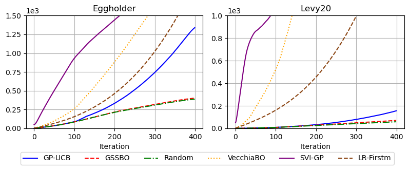
Figure 6: Cumulative time cost of algorithms 2 (in seconds).

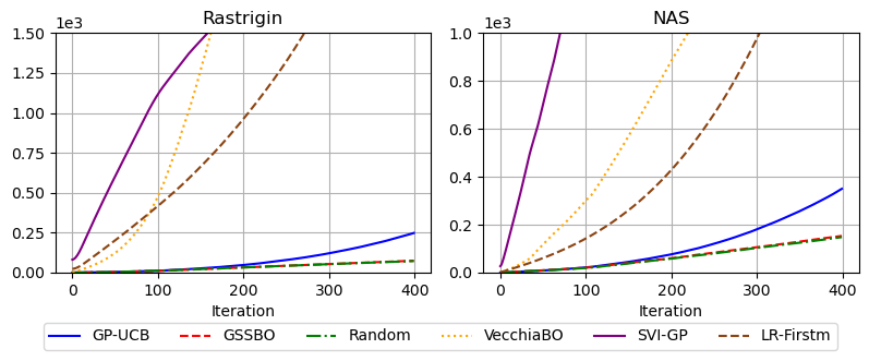
Figure 7: Cumulative time cost of algorithms 3 (in seconds).

Figure 8 illustrate a GP performance comparison between the GSSBO and the Standard GP-UCB, showing that the quantified differences between the two GPs are minimal. Figure 8 compares the root mean square error (RMSE) in 10,000 samples of the posterior mean functions of the two GPs at each iteration. The observed differences increase sub-linearly, indicating that the disparity between the two methods remains bounded, which is consistent with our theoretical analysis. These results suggest that the GSSBO effectively reduces computational costs while maintaining inference accuracy comparable to, or not significantly lower than, that of the Standard GP-UCB. This outcome validates the efficacy of our proposed approach.

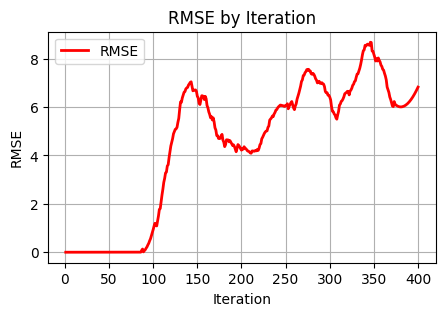
Figure 8: Inference gap between GSSBO and GP-UCB.

References

- Ahmed et al. (2016) Ahmed, M. O., Shahriari, B., and Schmidt, M. Do we need “harmless” bayesian optimization and “first-order” bayesian optimization. NIPS BayesOpt, 5:21, 2016.
- Aljundi et al. (2019) Aljundi, R., Lin, M., Goujaud, B., and Bengio, Y. Gradient based sample selection for online continual learning. Advances in neural information processing systems, 32, 2019.
- Bilal et al. (2020) Bilal, M., Serafini, M., Canini, M., and Rodrigues, R. Do the best cloud configurations grow on trees? an experimental evaluation of black box algorithms for optimizing cloud workloads. 2020.
- Binois & Wycoff (2022) Binois, M. and Wycoff, N. A survey on high-dimensional gaussian process modeling with application to bayesian optimization. ACM Transactions on Evolutionary Learning and Optimization, 2(2):1–26, 2022.
- Chen et al. (2018) Chen, C., Zhang, R., Wang, W., Li, B., and Chen, L. A unified particle-optimization framework for scalable bayesian sampling. arXiv preprint arXiv:1805.11659, 2018.
- Daulton et al. (2020) Daulton, S., Balandat, M., and Bakshy, E. Differentiable expected hypervolume improvement for parallel multi-objective bayesian optimization. Advances in Neural Information Processing Systems, 33:9851–9864, 2020.
- Daulton et al. (2021) Daulton, S., Balandat, M., and Bakshy, E. Parallel bayesian optimization of multiple noisy objectives with expected hypervolume improvement. Advances in Neural Information Processing Systems, 34:2187–2200, 2021.
- Drineas et al. (2005) Drineas, P., Mahoney, M. W., and Cristianini, N. On the nyström method for approximating a gram matrix for improved kernel-based learning. journal of machine learning research, 6(12), 2005.
- Dua & Graff (2017) Dua, D. and Graff, C. Uci machine learning repository, 2017. URL http://archive.ics.uci.edu/ml.
- Eriksson et al. (2019) Eriksson, D., Pearce, M., Gardner, J., Turner, R. D., and Poloczek, M. Scalable global optimization via local bayesian optimization. Advances in neural information processing systems, 32, 2019.
- Frazier (2018) Frazier, P. I. A tutorial on bayesian optimization. arXiv preprint arXiv:1807.02811, 2018.
- Garnett (2023) Garnett, R. Bayesian optimization. Cambridge University Press, 2023.
- González et al. (2016) González, J., Dai, Z., Hennig, P., and Lawrence, N. Batch bayesian optimization via local penalization. In Artificial intelligence and statistics, pp. 648–657. PMLR, 2016.
- Guyon & Elisseeff (2003) Guyon, I. and Elisseeff, A. An introduction to variable and feature selection. Journal of machine learning research, 3(Mar):1157–1182, 2003.
- Hastie (2009) Hastie, T. The elements of statistical learning: Data mining, inference, and prediction, 2009.
- Hensman et al. (2013) Hensman, J., Fusi, N., and Lawrence, N. D. Gaussian processes for big data. arXiv preprint arXiv:1309.6835, 2013.
- Jimenez & Katzfuss (2023) Jimenez, F. and Katzfuss, M. Scalable bayesian optimization using vecchia approximations of gaussian processes. In International Conference on Artificial Intelligence and Statistics, pp. 1492–1512. PMLR, 2023.
- Kandasamy et al. (2016) Kandasamy, K., Dasarathy, G., Oliva, J. B., Schneider, J., and Póczos, B. Gaussian process bandit optimisation with multi-fidelity evaluations. Advances in neural information processing systems, 29, 2016.
- Kim et al. (2021) Kim, J., McCourt, M., You, T., Kim, S., and Choi, S. Bayesian optimization with approximate set kernels. Machine Learning, 110:857–879, 2021.
- Lawrence et al. (2002) Lawrence, N., Seeger, M., and Herbrich, R. Fast sparse gaussian process methods: The informative vector machine. Advances in neural information processing systems, 15, 2002.
- Leibfried et al. (2020) Leibfried, F., Dutordoir, V., John, S., and Durrande, N. A tutorial on sparse gaussian processes and variational inference. arXiv preprint arXiv:2012.13962, 2020.
- McIntire et al. (2016) McIntire, M., Ratner, D., and Ermon, S. Sparse gaussian processes for bayesian optimization. In UAI, volume 3, pp. 4, 2016.
- Narendra & Fukunaga (1977) Narendra and Fukunaga. A branch and bound algorithm for feature subset selection. IEEE Transactions on computers, 100(9):917–922, 1977.
- Penubothula et al. (2021) Penubothula, S., Kamanchi, C., and Bhatnagar, S. Novel first order bayesian optimization with an application to reinforcement learning. Applied Intelligence, 51(3):1565–1579, 2021.
- Quinlan (1986) Quinlan, J. R. Induction of decision trees. Machine learning, 1:81–106, 1986.
- Rahimi & Recht (2007) Rahimi, A. and Recht, B. Random features for large-scale kernel machines. Advances in neural information processing systems, 20, 2007.
- Rana et al. (2017) Rana, S., Li, C., Gupta, S., Nguyen, V., and Venkatesh, S. High dimensional bayesian optimization with elastic gaussian process. In International conference on machine learning, pp. 2883–2891. PMLR, 2017.
- Schulz et al. (2018) Schulz, E., Speekenbrink, M., and Krause, A. A tutorial on gaussian process regression: Modelling, exploring, and exploiting functions. Journal of mathematical psychology, 85:1–16, 2018.
- Srinivas et al. (2009) Srinivas, N., Krause, A., Kakade, S. M., and Seeger, M. Gaussian process optimization in the bandit setting: No regret and experimental design. arXiv preprint arXiv:0912.3995, 2009.
- Tamiya & Yamasaki (2022) Tamiya, S. and Yamasaki, H. Stochastic gradient line bayesian optimization for efficient noise-robust optimization of parameterized quantum circuits. npj Quantum Information, 8(1):90, 2022.
- Wang & Ng (2020) Wang, S. and Ng, S. H. Partition-based bayesian optimization for stochastic simulations. In 2020 Winter Simulation Conference (WSC), pp. 2832–2843. IEEE, 2020.
- Wang et al. (2023) Wang, X., Jin, Y., Schmitt, S., and Olhofer, M. Recent advances in bayesian optimization. ACM Computing Surveys, 55(13s):1–36, 2023.
- Wang et al. (2016) Wang, Z., Hutter, F., Zoghi, M., Matheson, D., and De Feitas, N. Bayesian optimization in a billion dimensions via random embeddings. Journal of Artificial Intelligence Research, 55:361–387, 2016.
- Wei et al. (2015) Wei, K., Iyer, R., and Bilmes, J. Submodularity in data subset selection and active learning. In International conference on machine learning, pp. 1954–1963. PMLR, 2015.
- Williams & Seeger (2000) Williams, C. and Seeger, M. Using the nyström method to speed up kernel machines. Advances in neural information processing systems, 13, 2000.
- Wu & Frazier (2016) Wu, J. and Frazier, P. The parallel knowledge gradient method for batch bayesian optimization. Advances in neural information processing systems, 29, 2016.
- Yang et al. (2022) Yang, S., Xie, Z., Peng, H., Xu, M., Sun, M., and Li, P. Dataset pruning: Reducing training data by examining generalization influence. arXiv preprint arXiv:2205.09329, 2022.
- Zhang & Rodgers (2024) Zhang, M. and Rodgers, C. T. Bayesian optimization of gradient trajectory for parallel-transmit pulse design. Magnetic Resonance in Medicine, 91(6):2358–2373, 2024.
- Zhu (2016) Zhu, R. Gradient-based sampling: An adaptive importance sampling for least-squares. Advances in neural information processing systems, 29, 2016.