Efficient Formal Verification of Quantum Error Correcting Programs

Abstract.

Quantum error correction (QEC) is fundamental for suppressing noise in quantum hardware and enabling fault-tolerant quantum computation. In this paper, we propose an efficient verification framework for QEC programs. We define an assertion logic and a program logic specifically crafted for QEC programs and establish a sound proof system. We then develop an efficient method for handling verification conditions (VCs) of QEC programs: for Pauli errors, the VCs are reduced to classical assertions that can be solved by SMT solvers, and for non-Pauli errors, we provide a heuristic algorithm. We formalize the proposed program logic in Coq proof assistant, making it a verified QEC verifier. Additionally, we implement an automated QEC verifier, Veri-QEC, for verifying various fault-tolerant scenarios. We demonstrate the efficiency and broad functionality of the framework by performing different verification tasks across various scenarios. Finally, we present a benchmark of 14 verified stabilizer codes.

1. Introduction

Beyond the current noisy intermediate scale quantum (NISQ) era (Preskill, 2018), fault-tolerant quantum computation is an indispensable step towards scalable quantum computation. Quantum error correcting (QEC) codes serve as a foundation for suppressing noise and implementing fault-tolerant quantum computation in noisy quantum hardware. There have been more and more experiments illustrating the implementation of quantum error correcting codes in real quantum processors (Ryan-Anderson et al., 2021; Zhao et al., 2022; Acharya et al., 2023; Bluvstein et al., 2024; Bravyi et al., 2024). These experiments show the great potential of QEC codes to reduce noise. Nevertheless, the increasingly complex QEC protocols make it crucial to verify the correctness of these protocols before deploying them.

There have been several verification techniques developed for QEC programs. Numerical simulation, especially stabilizer-based simulation (Aaronson and Gottesman, 2004; Anders and Briegel, 2006; Gidney, 2021) is extensively used for testing QEC programs. While stabilizer-based simulations can efficiently handle QEC circuits with only Clifford operations  (Nielsen and Chuang, 2010) compared to general methods (Xu et al., 2023), showing the effectiveness and correctness of QEC circuits still requires millions or even trillions of test cases, which is the main bottleneck (Gidney, 2021). Recently, symbolic execution (Fang and Ying, 2024) has also been applied to verify QEC programs. It is an automated approach designed to handle a large number of test cases and is primarily intended for bug reporting. However, it has limited functionality, such as the inability to reason about non-Clifford gates or propagation errors, and it remains slow when verifying correct instances.

Program logic is another appealing verification technique. It naturally handles a class of instances simultaneously by expressing and reasoning about rich specifications in a mathematical way (Grout, 2011). Two recent works pave the way for using Hoare-style program logic for reasoning about QEC programs. Both works leverage the concept of stabilizer, which is critical in current QEC codes to develop their programming models. Sundaram et al. (Sundaram et al., 2022) established a lightweight Hoare-like logic for quantum programs that treat stabilizers as predicates. Wu et al. (Wu et al., 2021; Wu, 2024) studied the syntax and semantics of QEC programs by employing stabilizers as first-class objects. They proposed a program logic designed for verifying QEC programs with fixed operations and errors. Yet, at this moment, these approaches do not achieve usability for verifying large-scale QEC codes with complicated structures, in particular for real scenarios of errors that appear in fault-tolerant quantum computation.

Technical challenge

There are still critical challenges to the efficient verification of large-scale QEC programs, as summarized below.

• A suitable hybrid program logic supporting backward reasoning. QEC codes are designed to correct possible errors, making error modeling crucial for verification. To this end, it is necessary to introduce classical variables to describe errors and measurement outcomes, as well as properties like the maximum number of correctable errors. Backward reasoning is then desired since it gives a simple but complete rule for classical assignment, while forward reasoning needs additional universal quantifiers to ensure completeness. As discussed in (Unruh, 2019a) and illustrated in Example 3.3, interpreting $\vee$ as classical disjunction suffers from the incompleteness problem even for QEC codes, making it necessary to choose quantum logic as base logic, where, $\vee$ is interpreted as the sum of subspaces.

• Proving verification conditions generated by program logic. Traditionally, after annotating the program, the program logic will generate verification conditions (entailment of assertion formulas). A complete and rigorous approach is to use formal proofs; however, this requires significant human effort. Another approach is to use efficient solvers to achieve automatic proofs. Unfortunately, quantum logic lacks efficient tools similar to SMT solvers: systematically handling quantum logic has been a longstanding challenge. On the one hand, the continuity of subspaces makes brute-force search ineffective, while on the other hand, the lack of distributive laws makes finding a (canonical) normal form particularly difficult. It remains unknown if assertion formulas for QEC codes can be efficiently processed.

Contributions

Figure 1. Overall structure of our verification framework for QEC programs.

We propose a formal verification framework, summarized in Fig. 1, by proposing theoretical solutions to the above challenges, together with two implementations, (i) the Coq-based verified QEC verifier and (ii) the SMT-based automatic QEC verifier Veri-QEC, that ensure and illustrate the effectiveness of our theory. In detail, we contribute:

• Assertion logic and program logic (Section 3 and 4). Following (Sundaram et al., 2022; Wu et al., 2021), we use Pauli expressions as atomic propositions and interpret them as the $+1$-eigenspace of the corresponding Pauli operator. We additionally introduce classical variables and interpret logical connectives based on quantum logic, e.g., interpreting $\vee$ as the sum of subspaces rather than as a union. Adopting the semantics for classical-quantum from (Feng and Ying, 2021), we establish a sound proof system for quantum programs.

• Efficient handling of verification condition of QEC code (Section 5). The verification condition generated by a QEC code is typically of the form

  (1) $$\left(P_{1}\wedge\dots\wedge P_{n}\right)\wedge\Phi_{c}\models\bigvee\nolimits_{\mathbf{s}\in\{0,1\}^{n}}\left((-1)^{f_{1}(\mathbf{s})}P_{1}^{\prime}\wedge\dots\wedge(-1)^{f_{n}(\mathbf{s})}P_{n}^{\prime}\right),$$

  where $P_{i},P_{i}^{\prime}$ are Pauli expressions and $\Phi_{c}$ is a classical assertion. Progressing from simple to complex, we deal with the following cases: 1). $\{P_{i}^{\prime}\}\subseteq\{P_{j}\}$. Then it is equivalent to compare phase, which can be efficiently solved by an SMT solver. 2). All $P_{i}$ and $P_{j}^{\prime}$ commute. Then employ the fact that $P_{i}^{\prime}=(-1)^{a_{i}}\prod_{k\in K_{i}}P_{k}$ since $\{P_{i}\}$ is a minimal generating set and $P\wedge Q=P\wedge QP$ (Sundaram et al., 2022) to reduce it to case 1). 3). A non-commuting pair $P_{i}$ and $P_{j}^{\prime}$ exists. Then a heuristic algorithm is proposed to recursively eliminate $P_{j}^{\prime}$ from $\{P_{i}^{\prime}\}$ based on the facts $(P\wedge Q)\vee(\neg P\wedge Q)=Q$ if $P$ commute with $Q$, and finally reduce it to case 2).

• A verified QEC verifier (Section 6). We formalize our program logic in Coq proof assistant (The Coq Development Team, 2022) based on CoqQ (Zhou et al., 2023), i.e., proving the soundness of the proof system. This enhances confidence in the designed program logic. As a byproduct, this also allows us to manually formalize pen-and-paper proofs of scalable codes.

• Automatic QEC verifier Veri-QEC (Section 6 and 7). Veri-QEC is a practical tool developed in Python with the aid of Z3 and CVC5 SMT solvers (de Moura and Bjørner, 2008; Barbosa et al., 2022). Veri-QEC supports verification in various scenarios, from standard errors to propagation errors or errors in correction steps, and from one cycle of QEC code to fault-tolerant implementation of small logical circuits. We examine Veri-QEC on $14$ QEC codes selected from the stabilizer code family with $5-361$ qubits and perform different verification tasks based on the type of code and distance. Typical performance on surface codes includes: general verification for all error configurations up to $121$ qubits within $\sim 200$ minutes, and partial verification for user-provided error constraints up to $361$ qubits within $\sim 100$ minutes.

Comparison to existing works

Here we compare our work with works related to verifying QEC programs and leave the general discussion of related works in Section 8. Thanks to the efficiency of the stabilizer formalism in describing Clifford operations used in QEC programs, several works (Rand et al., 2021a; Wu et al., 2021; Wu, 2024; Rand et al., 2021b; Sundaram et al., 2022) utilize stabilizers as assertions in quantum programs. Among them, Rand et al. (2021a, b) built stabilizer formalism by designing a type system of Gottesman types, upon which Sundaram et al. (2022) further established a Hoare-like logic to characterize quantum programs consisting of Clifford gates, $T$ gate and measurements. The proof system was built in forward reasoning; thus the disjoint union ‘$\uplus$’ is employed to describe the post-measurement state. Wu et al. (2021) focused more on QEC. They designed a programming language with a stabilizer constructor in the syntax, specifically for QEC programs. This programming language faithfully captures the implementation of QEC protocols. To verify the correctness of QEC programs more efficiently while ensuring the accurate characterization of their properties, they designed an assertion logic using sums of stabilizers as atomic propositions and classical logical connectives. Given fixed operations, errors, and exact results of the decoder, this framework can effectively prove the correctness of a given QEC program.

Compared with prior works, our verification framework stands out by incorporating classical variables into both programs and assertions. Our assertion language enables simultaneous reasoning about properties of subspaces and a family of quantum states, such as logical computational basis states, which previous QEC program logic could only handle individually. Together with the classical variables in the program, our framework can model and verify the conditions of errors that previous work cannot reason about, e.g. the maximum correctable number of errors. Our program logic provides strong flexibility and efficiency to insert errors anywhere in the QEC program, such as before and after logic operators and within correction steps, and then verify the correctness. This capability is crucial for the subsequent step of verifying the implementation of fault-tolerant quantum computing.

2. Motivating example: The Steane code

We introduce a motivating example, the Steane code, which is widely used in quantum computers (Nigg et al., 2014; Ryan-Anderson et al., 2022; Bluvstein et al., 2022, 2024) to construct quantum circuits. A recent work (Bluvstein et al., 2024) demonstrates the use of Steane code to implement fault-tolerant logical algorithms in reconfigurable neutral-atom arrays. We aim to demonstrate the basic concepts of our formal verification framework through the verification of Steane code.

2.1. Basic Notations and Concepts

Quantum state.

Any state $|\psi\rangle$ of quantum bit (qubit) can be represented by a two-dimensional vector $\left(\begin{smallmatrix}\alpha\\ \beta\end{smallmatrix}\right)$ with $\alpha,\beta\in\mathbb{C}$ satisfying $|\alpha|^{2}+|\beta|^{2}=1$. Frequently used states include computational bases $|0\rangle\triangleq\left(\begin{smallmatrix}1\\ 0\end{smallmatrix}\right)$ and $|1\rangle\triangleq\left(\begin{smallmatrix}0\\ 1\end{smallmatrix}\right)$, and $|\pm\rangle=\frac{1}{\sqrt{2}}(|0\rangle\pm|1\rangle)$. The computational basis of an n-qubit system is $|\mathbf{s}\rangle\triangleq|s_{1}s_{2}\cdots s_{n}\rangle$ where $\mathbf{s}$ is a bit string, and any state $|\psi\rangle$ is a superposition $|\psi\rangle=\sum_{\mathbf{s}\in\{0,1\}^{n}}a_{\mathbf{s}}|\mathbf{s}\rangle$.

Unitary operator.

The evolution of a (closed) quantum system is modeled as a unitary operator, aka quantum gate for qubit systems. Here we list some of the commonly used quantum gates:

$$I=\begin{pmatrix}1&0\\ 0&1\end{pmatrix}\quad X=\begin{pmatrix}0&1\\ 1&0\end{pmatrix}\quad Y=\begin{pmatrix}0&-i\\ i&0\end{pmatrix} \quad Z=\begin{pmatrix}1&0\\ 0&-1\end{pmatrix}\quad H=\frac{1}{\sqrt{2}}\begin{pmatrix}1&1\\ 1&-1\end{pmatrix}\quad S=\begin{pmatrix}1&0\\ 0&i\end{pmatrix}$$

$$T=\begin{pmatrix}1&0\\ 0&e^{\frac{i\pi}{4}}\end{pmatrix}\quad CNOT=\begin{pmatrix}1&0&0&0\\ 0&1&0&0\\ 0&0&0&1\\ 0&0&1&0\end{pmatrix}\quad CZ=\begin{pmatrix}1&0&0&0\\ 0&1&0&0\\ 0&0&1&0\\ 0&0&0&-1\end{pmatrix}\quad iSWAP=\begin{pmatrix}1&0&0&0\\ 0&0&-i&0\\ 0&-i&0&0\\ 0&0&0&1\end{pmatrix}$$

The evolution is computed by matrix multiplication, for example, $H$ gate transform $|0\rangle$ to $H|0\rangle=\frac{1}{\sqrt{2}}\left(\begin{smallmatrix}1&1\\ 1&-1\end{smallmatrix}\right)\left(\begin{smallmatrix}1\\ 0\end{smallmatrix}\right)=\frac{1}{\sqrt{2}}\left(\begin{smallmatrix}1\\ 1\end{smallmatrix}\right)=|+\rangle$.

Projective measurement.

We here consider the boolean-valued projective measurement $M=\{P_{0},P_{1}\}$ with projections $P_{0}$ and $P_{1}$ such that $P_{0}+P_{1}=I$. Performing $M$ on a given state $|\psi\rangle$, with probability $p_{m}=|P_{m}|\psi\rangle|^{2}$ we get $m$ and post-measurement state $\frac{P_{m}|\psi\rangle}{\sqrt{p_{m}}}$ for $m=0,1$.

Pauli group and Clifford gate.

The Pauli group on $n$ qubits $\mathcal{P}_{n}$ consists of all Pauli strings $g$ which are represented by the tensor product of $n$ Pauli or identity matrices with multiplicative factor $\pm 1,\pm i$, i.e., $i^{t}p_{1}\otimes\cdots\otimes p_{n}$, where $p_{i}\in\{I,X,Y,Z\},t\in\{0,1,2,3\}$. A state $|\psi\rangle$ is stabilized by $g\in\mathcal{P}_{n}$ (or a subset $S\subseteq\mathcal{P}_{n}$) , if $g|\psi\rangle=|\psi\rangle$ (or $\forall\,g\in S,\ g|\psi\rangle=|\psi\rangle$). The measurement outcome of corresponding projective measurement $M_{g}$ is always $0$ iff $|\psi\rangle$ is a stabilizer state of $g$. A unitary $V$ is a Clifford gate, if for any Pauli string $g$, $VgV^{{\dagger}}$ is still a Pauli string. All Clifford gates form the Clifford group, and can be generated by $H,S$, and CNOT.

Stabilizer code.

An $[[n,k,d]]$ stabilizer code $\mathcal{C}$ is a subspace of the $n$-qubit state space, defined as the set (aka codespace) of states stabilized by an abelian subgroup $S$ (aka stabilizer group) of Pauli group $\mathcal{P}_{n}$, with a minimal representation in terms of $n-k$ independent and commuting generators $\langle g_{1},\dots,g_{n-k}\rangle$ requiring $-I\notin S$. The codespace of $\mathcal{C}$ is of dimension $2^{k}$ and thus able to encode $k$ logical qubits into $n$ physical qubits. With additional $k$ logical operators $\bar{Z}_{1},\cdots,\bar{Z}_{k}$ that are independent and commuting with each other and $S$, we can define a $k$-qubit logical state $|z_{1},\dots,z_{k}\rangle_{L}$ as the state stabilized by $\langle g_{1},\dots,g_{n-k},(-1)^{z_{1}}\bar{Z}_{1},\dots,(-1)^{z_{k}}\bar{Z}_{k}\rangle$ with $z_{i}\in\{0,1\}$. We can further construct $\bar{X}_{1},\dots,\bar{X}_{k}$ such that $\bar{X}_{i}$ commute with $g\in S$ and $\bar{X}_{i}\bar{Z}_{j}=(-1)^{\delta_{ij}}\bar{Z}_{j}\bar{X}_{i}$ for all $i,j\in\{1,\cdots,k\}$, and regard $\bar{Z}_{i}$ (or $\bar{X}_{i}$) as logical $Z$ (or $X$) gate acting on $i$-th logical qubit. $d$ is the code distance, i.e., the minimum (Hamming) weight of errors that can go undetected by the code.

2.2. The $[[7,1,3]]$ Steane code

The Steane code encodes a logical qubit using 7 physical qubits. The code distance is 3, therefore it is the smallest CSS code (Calderbank and Shor, 1996) that can correct any single-qubit Pauli error. The generators $g_{1},\ldots,g_{6}$, and logical operators $\bar{X}$ and $\bar{Z}$ of Steane code are as follows:

$$g_{1} \coloneq X_{1}X_{3}X_{5}X_{7} g_{2} \coloneq X_{2}X_{3}X_{6}X_{7} g_{3} \coloneq X_{4}X_{5}X_{6}X_{7} \bar{X} \coloneq X_{1}X_{2}X_{3}X_{4}X_{5}X_{6}X_{7}$$

$$g_{4} \coloneq Z_{1}Z_{3}Z_{5}Z_{7} g_{5} \coloneq Z_{2}Z_{3}Z_{6}Z_{7} g_{6} \coloneq Z_{4}Z_{5}Z_{6}Z_{7} \bar{Z} \coloneq Z_{1}Z_{2}Z_{3}Z_{4}Z_{5}Z_{6}Z_{7}.$$

In Table 1, we describe the implementations of logical Clifford operations and error correction procedures using the programming syntax introduced in Section 4.

As a running example, we analyze a one-round error correction process in the presence of single-qubit Pauli $Y$ errors, as well as the Hadamard $H$ error and $T$ error serving as instances of non-Pauli errors. First, we inject propagation errors controlled by Boolean-valued indicators $\{e_{pi}\}$ at the beginning. A propagation error simulates the leftover error from the previous error correction process, which must be considered and analyzed to achieve large-scale fault-tolerant computing. Next, a logical operation $H$ is applied followed by the standard error injection controlled by indicators $\{e_{i}\}$. Formally, $[e_{i}]q_{i}\,*\!\!=U$ means applying the error $U$ on $q_{i}$ if $e_{i}=1$, and skipping otherwise. Afterwards, we measure the system according to generators of the stabilizer group, compute the decoding functions $f_{x,i}$ and $f_{z,i}$, and finally perform correction operations. The technical details of the program can be found in Section 5.2 and Appendix C.

Table 1. Program Implementations of logical operation and error correction using a 7-qubit Steane code

Logical Operation		Error Correction
	Command	Explanation	Steane$(E)$-H  $E\in\{Y,H,T\}$
H	$\mathbf{for}\ i\in 1\dots 7\ \mathbf{do}\$	Propagation Error	$\mathbf{for}\ i\in 1\dots 7\ \mathbf{do}\ [e_{pi}]q_{i}\,*\!\!=E\ \mathbf{end}$
	$\quad q_{i}\,*\!\!=H\ \mathbf{end}$	Logical operation H	$\mathbf{for}\ i\in 1\dots 7\ \mathbf{do}\ q_{i}\,*\!\!=H\ \mathbf{end}$
S	$\mathbf{for}\ i\in 1\dots 7\ \mathbf{do}\$	Error injection	$\mathbf{for}\ i\in 1\dots 7\ \mathbf{do}\ [e_{i}]q_{i}\,*\!\!=E\ \mathbf{end}$
	$\quad q_{i}\,*\!\!=Z\fatsemi q_{i}\,*\!\!=S$	Syndrome meas	$\mathbf{for}\ i\in 1\dots 6\ \mathbf{do}\ s_{i}\coloneq\mathbf{meas}[g_{i}]\ \mathbf{end}$
	$\mathbf{end}$	Call decoder for Z	$z_{1},\ldots,z_{7}\coloneq f_{z}(s_{1},s_{2},s_{3})$
CNOT	$\mathbf{for}\ i\in 1\dots 7\ \mathbf{do}$	Call decoder for X	$x_{1},\ldots,x_{7}\coloneq f_{x}(s_{4},s_{5},s_{6})$
	$\quad q_{i},q_{i+7}\,*\!\!=CNOT$	Correction for X	$\mathbf{for}\ i\in 1\dots 7\ \mathbf{do}\ [x_{i}]q_{i}\,*\!\!=X\ \mathbf{end}$
	$\mathbf{end}$	Correction for Z	$\mathbf{for}\ i\in 1\dots 7\ \mathbf{do}\ [z_{i}]q_{i}\,*\!\!=Z\ \mathbf{end}$

The correctness formula for the program $\textbf{Steane}(E)-\textbf{H}$ can be stated as the Hoare triple::

(2) $$\left\{(\sum_{i=1}^{7}(e_{i}+e_{pi})\leq 1)\wedge((-1)^{b}\bar{X}\wedge g_{1}\wedge\cdots\wedge g_{6})\right\}\textbf{Steane}(E)-\textbf{H}\left\{(-1)^{b}\bar{Z}\wedge g_{1}\wedge\cdots\wedge g_{6}\right\}.$$

Here, $b$ is a parameter denoting the phase of the logical state, e.g., $b=0$ for initial state $|+\rangle_{L}$ (i.e., state stabilized by $\bar{X}\wedge g_{1}\wedge\cdots\wedge g_{6}$) and final state $|0\rangle_{L}$ (i.e., state stabilized by $\bar{Z}\wedge g_{1}\wedge\cdots\wedge g_{6}$). The correctness formula claims that if there is at most one $U$ error $(\sum_{i=1}^{7}(e_{i}+e_{pi})\leq 1)$, then the program transforms $|+\rangle_{L}$ to $|0\rangle_{L}$ (and $|-\rangle_{L}$ to $|1\rangle_{L}$), exactly the same as the error-free program that execute logical Hadamard gate $H$.

It appears hard to verify Eqn. (2) in previous works. (Wu et al., 2021; Wu, 2024) can only handle fixed Pauli errors while $\mathbf{Steane}$ involves non-Pauli errors $T$ with flexible positions. (Sundaram et al., 2022; Rand et al., 2021a) do not introduce classical variables and thus cannot represent flexible errors nor reason about the constraints or properties of errors. Fang and Ying (2024) cannot handle non-Clifford gates, since non-Clifford gates change the stabilizer generators (Pauli operators) into linear combinations of Pauli operators, which are beyond their scope.

In the following sections, we will verify Equation (2) by first deriving a precondition $A^{\prime}$ (see Equation (8) for $Y$ error and Equation (11) for $T$ error) by applying the inference rules from Figure LABEL:infer-rule, and then proving the verification condition $A\models A^{\prime}$ based on the techniques proposed in Section 5.1.

3. An Assertion logic for QEC programs

In this section, we introduce a hybrid classical-quantum assertion logic on which our verification framework is based.

3.1. Expressions

For simplicity, we do not explicitly provide the syntax of expressions of Boolean (denoted by $BExp$); see Appendix A.1 for an example. Their value is fully determined by the state of the classical memory $m\in\mathtt{CMem}$, which is a map from variable names to their values. Given a state $m$ of the classical memory, we write $\llbracket\cdot\rrbracket_{m}$ for the semantics of basic expressions in state $m$.

A special class of expressions was introduced by (Wu, 2024; Sundaram et al., 2022), namely Pauli expressions. In particular, for reasoning about QEC codes with $T$ gates, Sundaram et al. (2022) suggests extending basic Pauli groups with addition and scalar multiplication with factor from the ring

$$\mathbb{Z}[1/\sqrt{2}]\triangleq\{\,x+y/\sqrt{2}\mid x,y\in\mathbb{Z}\,\}=\{\,(x+y\sqrt{2})/2^{t}\mid t\in\mathbb{N},x,y\in\mathbb{Z}\,\}$$

We adopt a similar syntax of expressions in the ring $\mathbb{Z}[\frac{1}{\sqrt{2}}]$ and Pauli expressions for describing generators of stabilizer groups:

(3) $$SExp: S \Coloneqq{}(-1)^{b}\mid\sqrt{2}\mid S/2^{t}\mid S_{1}+S_{2}\mid-S\mid S_{1}S_{2} \mbox{syntax for ring $\mathbb{Z}[\frac{1}{\sqrt{2}}]$}.$$

(4) $$PExp: P \Coloneqq{}p_{r}\mid sP\mid P_{1}P_{2}\mid P_{1}+P_{2} s\in SExp$$ syntax for Pauli group with .

In $SExp$, $b$ is a Boolean expression and $t$ is an expression of natural numbers. In $PExp$, $p_{r}$ is an elementary gate defined as $p\in\{X,Y,Z\}$ with $r$ being a constant natural number indicating the qubit that $p$ acts on. $SExp$ and $PExp$ are interpreted inductively as follows:

$$\llbracket(-1)^{b}\rrbracket_{m}\triangleq(-1)^{\llbracket b\rrbracket_{m}},\quad\llbracket\sqrt{2}\rrbracket_{m}\triangleq\sqrt{2},\quad\llbracket s/2^{t}\rrbracket_{m}\triangleq\frac{\llbracket s\rrbracket_{m}}{2^{\llbracket t\rrbracket_{m}}},$$

$$\llbracket s_{1}+s_{2}\rrbracket_{m}\triangleq\llbracket s_{1}\rrbracket_{m}+\llbracket s_{2}\rrbracket_{m},\quad\llbracket-s\rrbracket_{m}\triangleq-\llbracket s\rrbracket_{m},\quad\llbracket s_{1}s_{2}\rrbracket_{m}\triangleq\llbracket s_{1}\rrbracket_{m}\llbracket s_{2}\rrbracket_{m}$$

$$\llbracket p_{r}\rrbracket_{m}\triangleq I_{1}\otimes\cdots\otimes I_{r-1}\otimes p_{r}\otimes I_{r+1}\otimes\cdots\otimes I_{n}$$

$$\llbracket sP\rrbracket_{m}=\llbracket s\rrbracket_{m}\llbracket P\rrbracket_{m},\quad\llbracket P_{1}P_{2}\rrbracket_{m}\triangleq\llbracket P_{1}\rrbracket_{m}\llbracket P_{2}\rrbracket_{m},\quad\llbracket P_{1}+P_{2}\rrbracket_{m}\triangleq\llbracket P_{1}\rrbracket_{m}+\llbracket P_{2}\rrbracket_{m}.$$

Here, $p_{r}$ is interpreted as a global gate by lifting it to the whole system, with $\otimes$ being the tensor product of linear operators, i.e., the Kronecker product if operators are written in matrix form. Such lifting is also known as cylindrical extension, and we sometimes omit explicitly writing out it. Note that it is redundant to introduce the syntax of the tensor product $p_{r_{1}}\otimes p_{r_{2}}$ with different $r_{1},r_{2}$, since

$$\llbracket p_{r_{1}}\otimes p_{r_{2}}\rrbracket_{m}=I_{1}\otimes\cdots\otimes I_{r_{1}-1}\otimes p_{r_{1}}\otimes I_{r_{1}+1}\otimes\cdots\otimes I_{r_{2}-1}\otimes p_{r_{2}}\otimes I_{r_{2}+1}\cdots\otimes I_{n}=\llbracket p_{r_{1}}p_{r_{2}}\rrbracket_{m}$$

if $r_{1}<r_{2}$.

One primary concern of Pauli expression syntax lies in its closedness under the unitary transformations Clifford + $T$ as claimed below. In fact, the factor $SExp$ is introduced to ensure the closedness under the $T$ gate.

Theorem 3.1 (Closedness of Pauli expression under Clifford + $T$, c.f. (Sundaram et al., 2022)).

For any Pauli expression $P$ defined in Equation (4) and single-qubit gate $U_{1}\in\{X,Y,Z,H,S,T\}$ acts on $q_{i}$ or two-qubit gate $U_{2}\in\{CNOT,CZ,iSWAP\}$ acts on $q_{i}q_{j}$, there exists another Pauli expression $Q\in PExp$, such that for all $m\in\mathtt{CMem}$, $\llbracket Q\rrbracket_{m}=U_{1i}^{\dagger}\llbracket P\rrbracket_{m}U_{1i}$ or $\llbracket Q\rrbracket_{m}=U_{2ij}^{\dagger}\llbracket P\rrbracket_{m}U_{2ij}$.

3.2. Assertion language

We further define the assertion language for QEC codes by adopting Boolean and Pauli expressions as atomic propositions. Pauli expressions characterize the stabilizer group and the subspaces stabilized by it, while Boolean expressions are employed to represent error properties.

Definition 3.2 (Syntax of assertion language).

(5) $$AExp:\quad A\Coloneqq{} b\in BExp\mid P\in PExp\mid\neg A\mid A\wedge A\mid A\vee A\mid A\Rightarrow A.$$

We interpret the assertion $A\in AExp$ as a map $\llbracket A\rrbracket:\mathtt{CMem}\rightarrow\mathcal{S}(\mathcal{H})$, where $\mathtt{CMem}$ is the set of classical states, $\mathcal{S}(\mathcal{H})$ is the set of subspaces in global Hilbert space $\mathcal{H}$. Formally, we define its semantics as:

$$\llbracket b\rrbracket_{m}\triangleq\left\{\begin{array}[]{ll}I_{\mathcal{H}}&\llbracket b\rrbracket_{m}=\mathbf{true}\\ 0_{\mathcal{H}}&\llbracket b\rrbracket_{m}=\mathbf{false}\end{array}\right.,\quad\llbracket P\rrbracket_{m}\triangleq\mathrm{span}\{|\psi\rangle:\llbracket P\rrbracket_{m}|\psi\rangle=|\psi\rangle\},\quad\llbracket\neg A\rrbracket_{m}\triangleq\llbracket A\rrbracket^{\bot}_{m},$$

$$\llbracket A_{1}\wedge A_{2}\rrbracket_{m}\triangleq\llbracket A_{1}\rrbracket_{m}\wedge\llbracket A_{2}\rrbracket_{m},\quad\llbracket A_{1}\vee A_{2}\rrbracket_{m}\triangleq\llbracket A_{1}\rrbracket_{m}\vee\llbracket A_{2}\rrbracket_{m},\quad\llbracket A_{1}\Rightarrow A_{2}\rrbracket_{m}\triangleq\llbracket A_{1}\rrbracket_{m}\rightsquigarrow\llbracket A_{2}\rrbracket_{m}$$

Boolean expression is embedded as null space or full space depending on its boolean semantics. Pauli expression is interpreted as its +1-eigenspace (aka codespace), intuitively, this is the subspace of states that are stabilized by it. It is slightly ambiguous to use $\llbracket P\rrbracket$ for both semantics of $PExp$ and $AExp$, while it can be recognized from the context if $\llbracket P\rrbracket_{m}$ refers to operator ($PExp$) or subspace ($AExp$). For the rest of connectives, $\llbracket\cdot\rrbracket$ is a point-wise extension of quantum logic, i.e., ^⊥ as orthocomplement, $\wedge$ as intersection, $\vee$ as span of union, $\rightsquigarrow$ as Sasaki implication of subspaces, i.e., $a\rightsquigarrow b\triangleq\neg a\vee(a\wedge b)$. Sasaki implication degenerates to classical implication whenever $a$ and $b$ commute, and thus it is consistent with boolean expression, e.g., $\llbracket b_{1}\rightarrow b_{2}\rrbracket=\llbracket b_{1}\Rightarrow b_{2}\rrbracket$ where $\rightarrow$ is the boolean implication. See Appendix A.3 for more details.

3.3. Why Birkhoff-von Neumann quantum logic as base logic?

In this section, we will discuss the advantages of choosing the projection-based (Birkhoff-von Neumann) quantum logic as the base logic to verify QEC programs.

Quantum logic vs. Classical logic

A key difference is the interpretation of $\vee$, which is particularly useful for backward reasoning about $\mathbf{if}$-branches, as shown by rule (If) in Figure LABEL:infer-rule that aligns with its counterpart in classical Hoare logic. However, interpreting $\vee$ as the classical disjunction is barely applicable for backward reasoning about measurement-based $\mathbf{if}$-branches, as illustrated below.

Example 3.3 (Failure of backward reasoning about $\mathbf{if}$-branches with classical disjunction).

Consider a fragment of QEC program $S\equiv b\coloneq\mathbf{meas}[Z_{2}];\mathbf{if}\ b\ \mathbf{then}\ q_{2}\,*\!\!=X\ \mathbf{else}\ \mathbf{skip}\ \mathbf{end}$, which first detects possible errors by performing a computational measurement on $q_{2}$ and then corrects the error by flipping $q_{2}$ if it is detected. It can be verified that the output state is stabilized by $X_{1}\wedge Z_{2}$ (i.e., in state $\ket{+0}_{q_{1}q_{2}}$) after executing $S$, if the input state is stabilized by $X_{1}$ (i.e., in state $\ket{+}_{q_{1}}\ket{\psi}_{q_{2}}$ for arbitrary $|\psi\rangle$). This fact can be formalized by correctness formula

(6) $$\{X_{1}\}\ b\coloneq\mathbf{meas}[Z_{2}];\mathbf{if}\ b\ \mathbf{then}\ q_{2}\,*\!\!=X\ \mathbf{else}\ \mathbf{skip}\ \mathbf{end}\ \{X_{1}\wedge Z_{2}\}.$$

When deriving the precondition with rule (If) where $\vee$ is interpreted as classical disjunction, one can obtain the semantics of precondition as $\llbracket A_{0}\vee A_{1}\rrbracket^{\prime}=\llbracket A_{0}\rrbracket\cup\llbracket A_{1}\rrbracket=\{\ket{+0}_{q_{1}q_{2}},\ket{+1}_{q_{1}q_{2}}\}$, where $A_{0}\triangleq X_{1}\wedge Z_{2}$ and $A_{1}\triangleq X_{1}\wedge-Z_{2}$. This semantics of precondition is valid but far from fully characterizing all valid inputs mentioned earlier, i.e., states of the form $\ket{+}_{q_{1}}\ket{\psi}_{q_{2}}$ for arbitrary $|\psi\rangle$.

Quantum logic naturally addresses this failure, since the semantics of precondition is exactly the set of all valid input states: $\llbracket A_{0}\vee A_{1}\rrbracket=\mathrm{span}\{\llbracket A_{0}\rrbracket\vee\llbracket A_{1}\rrbracket\}=\{\alpha\ket{+0}_{q_{1}q_{2}}+\ket{+1}_{q_{1}q_{2}}:\alpha,\beta\in\mathbb{C}\}=\llbracket X_{1}\rrbracket$. As Theorem A.11 suggested, the rules (If) and (Meas) maintain the universality and completeness of reasoning about broader QEC codes.

Projection-based vs. satisfaction-based approach

Although quantum logic offers richer algebraic structures, it is limited in expressiveness compared to observable-based satisfaction approaches (D’hondt and Panangaden, 2006; Ying, 2012) and effect algebras (Foulis and Bennett, 1994; Kraus et al., 1983): it cannot express or reason about the probabilistic properties of programs. However, this limitation is tolerable for reasoning about QEC codes. On one hand, errors in QEC codes are discretized as Pauli errors and do not directly require modeling the probability. On the other hand, a QEC code can perfectly correct discrete errors with non-probabilistic constraints. Therefore, representing and reasoning about the probabilistic attributes of QEC codes is unnecessary.

3.4. Satisfaction Relation and Entailment

In this section, we first review the representation of program states and then define the satisfaction relation, which specifies when the program states meet the truth condition of the assertion under a given interpretation.

Quantum states as density operators.

The quantum system after a measurement is generally an ensemble of pure state $\{p_{i},|\psi_{i}\rangle\}$, i.e., the system is in $|\psi_{i}\rangle$ with probability $p_{i}$. It is more convenient to express quantum states as partial density operators instead of pure states (Nielsen and Chuang, 2010). Formally, we write $\rho\triangleq\sum_{i}p_{i}|\psi_{i}\rangle\langle\psi_{i}|\in\mathcal{D}(\mathcal{H})$, where $\langle\psi_{i}|$ is the dual state, i.e., the conjugate transpose of $|\psi_{i}\rangle$.

Classical-quantum states.

We follow (Feng and Ying, 2021) to define the program state in our language as a classical-quantum state $\mu:\mathtt{CMem}\rightarrow\mathcal{D}(\mathcal{H})$, which is a map from classical states to partial density operators over the whole quantum system. In particular, the singleton state, i.e., the classical state $m$ associated with quantum state $\rho$, is denoted by $(m,\rho)$.

Satisfaction relation.

A one-to-one correspondence exists between projective operators and subspace, i.e., $X=\{|\psi\rangle:\mathtt{P}_{X}|\psi\rangle=|\psi\rangle\}$. Therefore, there is a standard way to define the satisfaction relation in projection-based approach (Zhou et al., 2019; Unruh, 2019a), i.e., a quantum state $\rho$ satisfies a subspace $X$, written $\rho\models X$, if and only if $\mathrm{supp}(\rho)\subseteq X$, or equivalently, $\mathtt{P}_{X}\rho\mathtt{P}_{X}=\rho$ (or $\mathtt{P}_{X}\rho=\rho$) where $\mathtt{P}_{X}$ is the corresponding projective operation of $X$. The satisfaction relation of classical-quantum states is a point-wise lifting:

Definition 3.4 (Satisfaction relation).

Given a classical-quantum state $\mu$ and an assertion $A\in AExp$, the satisfaction relation is defined as: $\mu\models A$ iff for all $m\in\mathtt{CMem}$, $\mu(m)\models\llbracket A\rrbracket_{m}$.

The satisfaction relation faithfully characterizes the relationship of stabilizer generators and their stabilizer states, i.e., for a Pauli expression $P$, $|\psi\rangle\langle\psi|\models P$ iff $|\psi\rangle$ is a stabilizer state of $\llbracket P\rrbracket_{m}$ for any $m\in\mathtt{CMem}$. We further define the entailment between two assertions:

Definition 3.5 (Entailment).

For $A,B\in AExp$, the entailment and logical equivalence are:

1. $A$ entails $B$, denoted by $A\models B$, if for all classical-quantum states $\mu$, $\mu\models A$ implies $\mu\models B$.

2. $A$ and $B$ are logically equivalent, denoted by $A\mathrel{\reflectbox{{$\models$}}}\!\>\!\models B$, if $A\models B$ and $B\models A$.

The entailment relation is also a point-wise lifting of the inclusion of subspaces, i.e., $A\models B$ iff for all $m$, $\llbracket A\rrbracket_{m}\subseteq\llbracket B\rrbracket_{m}$. As a consequence, the proof systems of quantum logic remain sound if its entailment is defined by inclusion, e.g., a Hilbert-style proof system for $AExp$ is presented in Appendix A.4. In the (consequence) rule (Figure LABEL:infer-rule) , strengthening the precondition and weakening the postcondition are defined as entailment relations of assertions. Therefore, entailment serves as a basis for verification conditions, which are established according to the consequence rule.

To conclude this section, we point out that the introduction of our assertion language enables us to leverage the following observation in efficient QEC verification:

Observation 3.1.

Verifying the correctness of quantum programs requires verification for all states within the state space. By introducing phase factor $(-1)^{b}$ to Pauli expressions, we can circumvent the need to verify each state individually. Consider a QEC code in which a logical state $|b_{1}\cdots b_{k}\rangle_{L}$ is stabilized by the set of generators and logical operators $\langle g_{1},\cdots,g_{n-k},(-1)^{b_{1}}\bar{Z}_{1},\cdots,(-1)^{b_{k}}\bar{Z}_{k}\rangle$. We can simultaneously verify the correctness for all logical states from the set $\{|b_{1}\cdots b_{k}\rangle_{L}|b_{1},\cdots,b_{k}\in\{0,1\}\}$, without introducing exponentially many assertions.

4. A Programming Language for QEC Codes and Its Logic

In this section, we introduce our programming language and the program logic specifically designed for QEC programs.

4.1. Syntax and Semantics

The set of program commands $\mathit{Prog}$ is defined as follows:

$$\mathit{Prog}:\quad S\Coloneqq{} \mathbf{skip}\mid q_{i}\coloneq\ket{0}\mid q_{i}\,*\!\!=U_{1}\mid q_{i}q_{j}\,*\!\!=U_{2}$$ where:

$$x\coloneq e\mid x\coloneq\mathbf{meas}[P]\mid S\fatsemi S U_{1}\in\{X,Y,Z,H,S,T\}$$

$$\mathbf{if}\ b\ \mathbf{then}\ S\ \mathbf{else}\ S\ \mathbf{end}\mid\mathbf{while}\ b\ \mathbf{do}\ S\ \mathbf{end} U_{2}\in\{CNOT,CZ,iSWAP\}$$

where $\mathbf{skip}$ denotes the empty program, and $q_{i}\coloneq\ket{0}$ resets the $i$-th qubit to ground state $|0\rangle$. A restrictive but universal gate set is considered for unitary transformation, with single qubit gates from $\{X,Y,Z,H,S,T\}$ and two-qubit gates from $\{CNOT,CZ,iSWAP\}$, where $i$ and $j$, as the indexes of unitaries, are constants and $i\neq j$ for two-qubit gates. $x\coloneq e$ is the classical assignment. In quantum measurement $x\coloneq\mathbf{meas}[P]$, $P\in PExp$ is a Pauli expression which defines a projective measurement $\{M_{0}=\mathtt{P}_{\llbracket P\rrbracket_{m}},M_{1}=\mathtt{P}_{\llbracket P\rrbracket_{m}^{\bot}}\}$; after performing the measurement, the outcome is stored in classical variable $x$. $S\fatsemi S$ is the sequential composition of programs. In if/loop commands, guard $b\in BExp$ is a Boolean expression, and the execution branch is determined by its value $\llbracket b\rrbracket_{m}$.

Our language is a subset of languages considered in (Feng and Ying, 2021), and we follow the same theory of defining operational and denotational semantics. In detail, a classical-quantum configuration is a pair $\langle S,(m,\rho)\rangle$, where $S$ is the program that remains to be executed with extra symbol $\downarrow$ for termination, and $(m,\rho)$ the current singleton states of the classical memory and quantum system. The transition rules for each construct are presented in Figure 4.1. We can further define the induced denotational semantics $\llbracket S\rrbracket:(\mathtt{CMem}\times\mathcal{D}(\mathcal{H}))\rightarrow(\mathtt{CMem}\rightarrow\mathcal{D}(\mathcal{H}))$, which is a mapping from singleton states to classical-quantum states (Feng and Ying, 2021). We review the technical details in Appendix A.5.

(Skip) $$\langle\mathbf{skip},(m,\rho)\rangle\rightarrow\langle\downarrow,(m,\rho)\rangle\hskip 14.22636pt\mbox{(Init)}\ \langle q_{i}\coloneq|0\rangle,(m,\rho)\rangle\rightarrow\langle\downarrow,(m,\sum_{k=0,1}|0\rangle_{q_{i}}\langle k|\rho|k\rangle_{q_{i}}\langle 0|)\rangle$$

(Unit1) $$\langle q_{i}\,*\!\!=U,(m,\rho)\rangle\rightarrow\langle\downarrow,(m,U_{q_{i}}\rho U_{q_{i}}^{{\dagger}})\rangle\hskip 14.22636pt\mbox{(Unit2)}\ \langle q_{i}q_{j}\,*\!\!=U,(m,\rho)\rangle\rightarrow\langle\downarrow,(m,U_{q_{i,j}}\rho U_{q_{i,j}}^{{\dagger}})\rangle$$

(Assign) $$\langle x\coloneq e,(m,\rho)\rangle\rightarrow\langle\downarrow,(m[\llbracket e\rrbracket_{m}/x],\rho)\rangle\hskip 14.22636pt\mbox{(Meas)}\ \inference{M_{0}=\mathtt{P}_{\llbracket P\rrbracket_{m}},M_{1}=\mathtt{P}_{\llbracket P\rrbracket_{m}^{\bot}}}$$

(Seq) $$\inference{\langle S_{1},(m,\rho)\rangle\rightarrow\langle S_{1}^{\prime},(m^{\prime},\rho^{\prime})\rangle}{\hskip-5.69046pt\langle S_{1}\fatsemi S_{2},(m,\rho)\rangle\rightarrow\langle S_{1}^{\prime}\fatsemi S_{2},(m^{\prime},\rho^{\prime})\rangle\hskip-5.69046pt}\hskip 23.61583pt\mbox{(If-F)}\ \inference{\llbracket b\rrbracket_{m}=\mathbf{false}}{\hskip-5.69046pt\langle\mathbf{if}\ b\ \mathbf{then}\ S_{1}\ \mathbf{else}\ S_{0}\ \mathbf{end},(m,\rho)\rangle\rightarrow\langle S_{0},(m,\rho)\rangle\hskip-5.69046pt}$$

(While-F) $$\inference{\llbracket b\rrbracket_{m}=\mathbf{false}}{\hskip-5.69046pt\langle\mathbf{while}\ b\ \mathbf{do}\ S\ \mathbf{end},(m,\rho)\rangle\rightarrow\langle\downarrow,(m,\rho)\rangle\hskip-5.69046pt}\hskip 11.38092pt\mbox{(If-T)}\ \inference{\llbracket b\rrbracket_{m}=\mathbf{true}}{\hskip-5.69046pt\langle\mathbf{if}\ b\ \mathbf{then}\ S_{1}\ \mathbf{else}\ S_{0}\ \mathbf{end},(m,\rho)\rangle\rightarrow\langle S_{1},(m,\rho)\rangle\hskip-5.69046pt}$$

(While-T) $$\inference{\llbracket b\rrbracket_{m}=\mathbf{true}}{\langle\mathbf{while}\ b\ \mathbf{do}\ S\ \mathbf{end},(m,\rho)\rangle\rightarrow\langle S\fatsemi\mathbf{while}\ b\ \mathbf{do}\ S\ \mathbf{end},(m,\rho)\rangle}$$

Figure 2. Operational semantics for QEC programs

Expressiveness of the programming language

Our programming language supports Clifford + T gate set and Pauli measurements. Therefore, it is capable of expressing all possible quantum operations, in an approximate manner. The claim of expressiveness can be proved by the following observations:

1. Clifford + T is a universal gate set (Nielsen and Chuang, 2010). Thus, according to the Solovay-Kitaev theorem, any unitary $U$ can be approximated within error $\epsilon$ using $\Theta(\log^{c}(1/\epsilon))$ gates from this set.

2. Measurement in any computational basis $|m\rangle=|a_{1}a_{2}\cdots a_{n}\rangle$ is performed by the projector $\mathtt{P}_{m}=\frac{\Pi_{i=1}^{n}(I+(-1)^{a_{i}}Z_{i})}{2^{n}}$, which can be expressed using our measurement statements $x\coloneq\textbf{meas}[(-1)^{a_{i}}Z_{i}]$. Further, projective measurements augmented by unitary operations are sufficient to implement a general POVM measurement.

4.2. Correctness formula and proof system

Definition 4.1 (Correctness formula).

The correctness formula for QEC programs is defined by the Hoare triple $\{A\}S\{B\}$, where $S\in Prog$ is a QEC program, $A,B\in AExp$ are the pre- and post-conditions. A formula $\{A\}S\{B\}$ is valid in the sense of partial correctness, written as $\models\{A\}S\{B\}$, if for any singleton state $(m,\rho)$: $(m,\rho)\models A$ implies $\llbracket S\rrbracket(m,\rho)\models B$.

The proof system of QEC program is presented in Fig. LABEL:infer-rule. Most of the inference rules are directly inspired from (Ying, 2012; Zhou et al., 2019; Feng and Ying, 2021). We use $A[e/x]$ (or $A[e_{1}/x_{1},e_{2}/x_{2},\cdots]$) to denote the (simultaneous) substitution of variable $x$ or constant constructor $x\in\{X_{r},Y_{r},Z_{r}\}$ with expression $e$ in assertion $A$. Based on the syntax of our assertion language and program constructors, we specifically design the following rules:

• Rule (Init) for initialization. Previous works (Ying, 2012; Feng and Ying, 2021) do not present syntax for assertion language and give the precondition based on the calculation of semantics, which, however, cannot be directly expressed in $AExp$. We derive the rule (Init) from the fact that initialization can be implemented by a computational measurement followed by a conditional $X$ gate. As shown in the next section, the precondition is indeed the weakest precondition and semantically equivalent to the one proposed in (Zhou et al., 2019).

• Rules for unitary transformation. We provide the rules for Clifford + $T$ gates, controlled-Z ($CZ$) gate, as well as $iSWAP$ gate, which are easily implemented in superconducting quantum computers. It is interesting to notice that, even for two-qubit unitary gates, the pre-conditions can still be written as the substitution of elementary Pauli expressions.

Reasoning about Pauli errors

To model the possible errors occurring in the QEC program, we further introduce a syntax sugar $[b]q_{i}\,*\!\!=U$ for ‘$\mathbf{if}\ b\ \mathbf{then}\ q_{i}\,*\!\!=U\ \mathbf{else}\ \mathbf{skip}\ \mathbf{end}$’ command, which means if the guard $b$ is true then apply Pauli error $U\in\{X,Y,Z\}$ on $q$, otherwise skip. The corresponding derived rules are:

$$\hskip-8.5359pt\begin{array}[]{ll}\{A[(-1)^{b}Y_{i}/Y_{i},(-1)^{b}Z_{i}/Z_{i}]\}\ [b]q_{i}\,*\!\!=X\ \{A\}&\{A[(-1)^{b}X_{i}/X_{i},(-1)^{b}Z_{i}/Z_{i}]\}\ [b]q_{i}\,*\!\!=Y\ \{A\}\\[2.84544pt] \{A[(-1)^{b}X_{i}/X_{i},(-1)^{b}Y_{i}/Y_{i}]\}\ [b]q_{i}\,*\!\!=Z\ \{A\}.&\end{array}$$

Example 4.2 (Derivation of the precondition using the proof system).

Consider a fragment of QEC program which describes the error correction stage of 3-qubit repetition code: $\mathbf{for}\ i\in 1\dots 3\ \mathbf{do}\ [x_{i}]q_{i}\,*\!\!=X\ \mathbf{end}$. This program corrects possible $X$ errors indicated by $x_{i}$. Starting from the post-condition $Z_{1}Z_{2}\wedge Z_{2}Z_{3}\wedge(-1)^{b}Z_{1}$, we derive the weakest pre-condition for this program:

$$\{Z_{1}Z_{2}\wedge(-1)^{x_{3}}Z_{2}Z_{3}\wedge(-1)^{b}Z_{1}\} [x_{3}]q_{3}\,*\!\!=X\ \{Z_{1}Z_{2}\wedge Z_{2}Z_{3}\wedge(-1)^{b}Z_{1}\}$$

$$\{(-1)^{x_{2}}Z_{1}Z_{2}\wedge(-1)^{x_{3}+x_{2}}Z_{2}Z_{3}\wedge(-1)^{b}Z_{1}\} [x_{2}]q_{2}\,*\!\!=X\ \{Z_{1}Z_{2}\wedge(-1)^{x_{3}}Z_{2}Z_{3}\wedge(-1)^{b}Z_{1}\}$$

$$\{(-1)^{x_{2}+x_{1}}Z_{1}Z_{2}\wedge(-1)^{x_{3}+x_{2}}Z_{2}Z_{3}\wedge(-1)^{b+x_{1}}Z_{1}\} [x_{1}]q_{1}\,*\!\!=X\ \{(-1)^{x_{2}}Z_{1}Z_{2}\wedge(-1)^{x_{3}+x_{2}}Z_{2}Z_{3}\wedge(-1)^{b}Z_{1}\}$$

We break down the syntax sugar as a sequence of subprograms and use the inference rules for Pauli errors to derive the weakest pre-condition.

4.3. Soundness theorem

In this subsection, we present the soundness of our proof system and sketch the proofs.

Theorem 4.3 (Soundness).

The proof system presented in Figure LABEL:infer-rule is sound for partial correctness; that is, for any $A,B\in AExp$ and $S\in Prog$, $\vdash\{A\}S\{B\}$ implies $\models\{A\}S\{B\}$.

The soundness theorem can be proved in two steps. First of all, we provide the rigorous definition of the weakest liberal precondition $wlp.S.f_{B}$ for any program $S\in\mathit{Prog}$ and mapping $f_{B}:\mathtt{CMem}\rightarrow\mathcal{S}(\mathcal{H})$ and prove the correctness of this definition. Subsequently, we use structural induction to prove that for any $A,B\in AExp$ and $S\in Prog$ such that $\vdash\{A\}S\{B\}$, $\llbracket A\rrbracket\models wlp.S.\llbracket B\rrbracket$. Proofs are discussed in detail in Appendix A.7.

5. Verification Framework and a Case Study

Now we are ready to assemble assertion logic and program logic presented in the previous two section into a framework of QEC verification.

5.1. Verification Conditions

As Theorem A.12 suggests, all rules except for (While) and (Con) give the weakest liberal precondition with respect to the given postconditions. Then the standard procedure like the weakest precondition calculus can be used to verify any correctness formula $\{A\}S\{B\}$, as discussed in (ying2016foundations):

1. Obtain the expected precondition $A^{\prime}$ in $\{A^{\prime}\}S\{B\}$ by applying inference rules of the program logic backwards.

2. Generate and prove the verification condition (VC) $A\models A^{\prime}$ using the assertion logic.

Dealing with VC requires additional efforts, particularly in the presence of non-commuting pairs of Pauli expressions. However for QEC programs, there exists a general form of verification condition, which can be derived from the correctness formula:

Definition 5.1 (Correctness formula for QEC programs).

Consider a program $S=\textbf{Corr}(E)-\bar{U}$, which is generalized from the QEC program in Table 1. It operates on a stabilizer code with a minimal generating set $\{g_{1},\cdots,g_{n-k},\bar{L}_{n-k+1},\cdots,\bar{L}_{n}\}$ containing $n$ independent and commuting Pauli expressions. The correctness formula of this program can be expressed as follows:

(7) $$\left\{\bigwedge_{i}g_{i}\wedge\bigwedge_{j}\bar{L}_{j}\right\}\ S\ \left\{\bigwedge_{i}g_{i}\wedge\bigwedge_{j}\bar{U}\bar{L}_{j}\bar{U}^{{\dagger}}\right\}$$

The verification condition to be proven is derived from this correctness formula with the aid of inference rules, as demonstrated below:

(8) $$\Big{(}\bigwedge_{i}g_{i}\wedge\bigwedge_{j}\bar{L}_{j}\Big{)}\ \wedge P_{c}\models\bigvee_{\mathbf{s}\in\{0,1\}^{n-k}}\left(\bigwedge_{i}(-1)^{r_{i}(\mathbf{s})+h_{i}(\mathbf{e})}g_{i}^{\prime}\wedge\bigwedge_{j}(-1)^{r_{j}(\mathbf{s})+h_{j}(\mathbf{e})}\bar{L}_{j}^{\prime}\right),$$

In Equation (8), $P_{c}$ represents a classical assertion for errors, $i,j$ range over $\{1,\cdots,n-k\}$, $\{n-k+1,\cdots,n\}$ respectively, The vector $\mathbf{s}$ encapsulates all possible measurement outcomes (syndromes) and $\mathbf{e}$ represents the error configuration. The semantics of $g_{i},g_{i}^{\prime},\bar{L}_{j},\bar{L}_{j}^{\prime}$ are normal operators. The terms $r_{i}(\mathbf{s}),r_{j}(\mathbf{s})$ denote the sum of all corrections effective for the corresponding operators, while $h_{i}(\mathbf{e}),h_{j}(\mathbf{e})$ account for the total error effects on the operators caused by the injected errors. The details of derivation are provided in Appendix B.1.

Let us consider how to prove Eqn. (8) in the following three cases:

1. $\{g_{i}^{\prime}\}\subseteq\{g_{i}\}$ and $\{\bar{L}_{j}^{\prime}\}\subseteq\{\bar{L}_{j}\}$. The entailment is then equivalent to check $P_{c}\models\bigvee_{\mathbf{s}}\big{(}\bigwedge_{i}(r_{i}(\mathbf{s})+h_{i}(\mathbf{e})=0)\wedge\bigwedge_{j}(r_{j}(\mathbf{s})+h_{j}(\mathbf{e})=0)\big{)}$, which can be proved directly by SMT solvers.

2. All $g_{i},g_{i}^{\prime},\bar{L}_{j},\bar{L}_{j}^{\prime}$ commute with each other. Since $\{g_{i},\bar{L}_{j}\}$ is a minimal generating set, any $g_{i}^{\prime}$ or $\bar{L}_{j}^{\prime}$ can be written as the product of $\{g_{i},\bar{L}_{j}\}$ up to a phase $\pm 1$, e.g., $(-1)^{\alpha_{i}}g_{i}^{\prime}=\prod_{i\in\mathcal{I}_{i^{\prime}}}g_{i}\prod_{j\in\mathcal{J}_{j^{\prime}}}\bar{L}_{j}$, $(-1)^{\alpha_{j}}\bar{L}_{j}^{\prime}=\prod_{i\in\mathcal{I}_{i^{\prime}}}g_{i}\prod_{j\in\mathcal{J}_{j^{\prime}}}\bar{L}_{j}$, so the entailment is equivalent to check $P_{c}\models\bigvee_{\mathbf{s}}\big{(}\bigwedge_{i}(r_{i}(\mathbf{s})+h_{i}(\mathbf{e})=a_{i})\wedge\bigwedge_{j}(r_{j}(\mathbf{s})+h_{j}(\mathbf{e})=a_{j})\big{)}$.

3. There exist non-commuting pairs. We consider the case that the total errors are less than the code distance; furthermore, $g_{i}^{\prime}$ is ordered such that $g_{i}^{\prime}=Ug_{i}U^{\dagger}$ for some unitary $U$, which can be easily achieved by preserving the order of subterms during the annotation step (1). The key idea to address this issue involves eliminating all non-commuting terms on the right-hand side (RHS) and identifying a form that is logically equivalent to the RHS. We briefly discuss the steps of how to eliminate the non-commuting terms, as outlined below:

   1. Find the set $\mathcal{G}\subseteq\{g_{i}^{\prime}\}$ such that any element $g_{i}^{\prime}\in\mathcal{G}$ differs from $g_{i}$ up to a phase; Find the set $\mathcal{L}\subseteq\{\bar{L}_{j}^{\prime}\}$ such that $\bar{L}_{j}^{\prime}$ differs from $\bar{L}_{j}$ up to a phase.

   2. Update $\mathcal{G}$ and $\mathcal{L}$ by multiplying some $g_{i}^{\prime}\in\mathcal{G}$ onto those elements, until $\mathcal{L}$ is empty and any $g_{i}^{\prime}\in\mathcal{G}$ differs from $g_{i}$ in only one qubit.

   3. Replace those $g_{i}^{\prime}$ with $g_{i}$, and check if the phases of the remaining items are the same for all $2^{k}$ terms. If so, this problem can be reduced to the commuting case, since we can successfully use $(P\wedge Q)\vee(\neg P\wedge Q)=Q$ ($P$ and $Q$ commute with each other) to eliminate all non-commuting elements.

   To illustrate how our ideas work, we provide an concrete example in Section 5.2.2, which illustrates how to correct a single $T$ error in the Steane code.

Soundness of the methods.

After proposing the methods to handle the verification condition (VC), we now discuss the soundness of our methods case by case:

$\bullet$ Commuting case. If all $g_{i},g_{i}^{\prime},\bar{L}_{j},\bar{L}^{\prime}_{j}$ commute with each other, then the equivalence of the VC proposed in case (2) and Equation (8) can be guaranteed by the following proposition:

Proposition 5.2.

Given a verification condition of the form:

(9) $$\left((-1)^{b_{1}}P_{1}\wedge\dots\wedge(-1)^{b_{n}}P_{n}\right)\wedge P_{c}\models\bigvee_{\mathbf{s}}\left((-1)^{b_{1}^{\prime}}P_{1}^{\prime}\wedge\dots\wedge(-1)^{b_{n}^{\prime}}P_{n}^{\prime}\right)$$

where $\{(-1)^{b_{1}}P_{1},\dots,(-1)^{b_{n}}P_{n}\}$, $\{(-1)^{b_{1}^{\prime}}P_{1}^{\prime},\dots,(-1)^{b_{n}^{\prime}}P_{n}^{\prime}\}$ are independent and commuting generators of two stabilizer groups $S,S^{\prime}\subseteq\mathcal{G}_{n}$, $\mathcal{G}_{n}$ is the n-qubit Pauli group. $S$ and $S^{\prime}$ satisfy $-I\notin S,S^{\prime}$. If $\{P_{1},\dots,P_{n},P_{1}^{\prime},\dots,P_{n}^{\prime}\}$ commute with each other, then:

1. For all $i$, there exist a unique $\alpha_{i}\in\{0,1\}$ and $\{i_{j}\}\in 2^{[n]},s.t.(-1)^{\alpha_{i}}P_{i}^{\prime}=\Pi_{j}P_{i_{j}}$.

2. $P_{c}\models\bigwedge_{i=1}^{n}(b_{i}^{\prime}=\alpha_{i}+\sum_{j}b_{i_{j}})$ implies $A\models A^{\prime}$, where $A,A^{\prime}$ are left and right hand side of Expression (9).

The proof leverages the observation that any $P_{i}^{\prime}$ which commutes with all elements in a stabilizer group $S$ can be written as products of generators of $S$ (Nielsen and Chuang, 2010). We further use $P\wedge Q=QP$ to reformulate the LHS of Expression (9) and generate terms that differs from the RHS only by phases. The detailed proof of this proposition is postponed to Appendix B.2.

$\bullet$ Non-commuting case. The soundness of this case can be demonstrated by separately proving the soundness of step (a), (b) and step (c).

1. Step (a) and (b): Consider the check matrix $H$. If step (b) fails for some error configuration $\mathbf{e}$ with weight $w_{\mathbf{e}}\leq d-1$, then there exists a submatrix $H_{sub}$ of size $(n-k)\times w_{\mathbf{e}}$, with columns being the error locations. The rank of the submatrix is $r<w_{\mathbf{e}}$, leading to a contradiction with the definition of $d$ being the minimal weight of an undetectable error. This is because there exists another $\mathbf{e}^{\prime}$ whose support is within that of $\mathbf{e}$, and $H\mathbf{e}^{\prime}=0$.

2. Step (c): The soundness is straightforward since $(P\wedge Q)\vee(\neg P\wedge Q)=Q$ whenever $P$ and $Q$ commute, which is the only formula we use to eliminate non-commuting elements.

5.2. Case study: Steane code (continued)

To illustrate the general procedure of our verification framework, let us consider the 7-qubit Steane code presented in Section 2.2 with $Y$ and $T$ errors ($H$ errors is deferred to Appendix C.2).

5.2.1. Case I: Reasoning about Pauli $Y$ errors

We first verify the correctness of Steane code with Pauli $Y$ errors. We choose $Y$ error because its impact on stabilizer codes is equivalent to the composite effect of $X$ and $Z$ errors on the same qubit. In this scenario, the verification condition (VC) to be proved is generated from the precondition:.

(10) $$\left\{(\sum_{i=1}^{7}e_{i}\leq 1)\wedge((-1)^{b}\bar{Z}\wedge\bigwedge_{i=1}^{6}g_{i})\right\}\models\left\{\bigvee_{\mathbf{s}\in\{0,1\}^{6}}(-1)^{b+r_{7}(\mathbf{s})+h_{7}(\mathbf{e})}\bar{Z}\wedge\bigwedge_{i=1}^{6}(-1)^{r_{i}(\mathbf{s})+h_{i}(\mathbf{e})}g_{i}\right\}.$$

No changes occur in Pauli generators $\bar{Z}$ and $g_{i}$, therefore according to case (1) in the proof of Equation (8), the verification condition is equivalent with $P_{c}\sqsubseteq P_{c}^{\prime}$, where $P_{c}=\sum_{i=1}^{7}e_{i}\leq 1$, $P_{c}^{\prime}=\bigvee_{\mathbf{s}\in\{0,1\}^{6}}\bigwedge_{i=1}^{7}(r_{i}(\mathbf{s})+h_{i}(\mathbf{e})=0)$.

Table 2. Symbols and values appear in Equation (10)

Symbols	Values	Symbols	Values	Symbols	Values
$r_{7}(\mathbf{s})$	$\sum_{i=1}^{7}f_{z,i}$	$h_{7}(\mathbf{e})$	$\sum_{i=1}^{7}e_{i}$
$h_{1}(\mathbf{e})$, $h_{4}(\mathbf{e})$	$e_{1}+e_{3}+e_{5}+e_{7}$	$h_{2}(\mathbf{e})$, $h_{5}(\mathbf{e})$	$e_{2}+e_{3}+e_{6}+e_{7}$	$h_{3}(\mathbf{e})$, $h_{6}(\mathbf{e})$	$e_{4}+e_{5}+e_{6}+e_{7}$
$r_{1}(\mathbf{s})$	$f_{z,1}+f_{z,3}+f_{z,5}+f_{z,7}$	$r_{2}(\mathbf{s})$	$f_{z,2}+f_{z,3}+f_{z,6}+f_{z,7}$	$r_{3}(\mathbf{s})$	$f_{z,4}+f_{z,5}+f_{z,6}+f_{z,7}$
$r_{4}(\mathbf{s})$	$f_{x,1}+f_{x,3}+f_{x,5}+f_{x,7}$	$r_{5}(\mathbf{s})$	$f_{x,2}+f_{x,3}+f_{x,6}+f_{x,7}$	$r_{6}(\mathbf{s})$	$f_{x,4}+f_{x,5}+f_{x,6}+f_{x,7}$

We can prove the VC if the minimum-weight decoder $f$ satisfies $P_{f}$:

$$P_{f}\triangleq\Big{(}\sum_{i=1}^{7}x_{i}\leq\sum_{i=1}^{7}e_{i}\Big{)}\bigwedge\Big{(}\sum_{i=1}^{7}z_{i}\leq\sum_{i=1}^{7}e_{i}\Big{)}\bigwedge\Big{(}\bigwedge_{i=1}^{6}(r_{i}(\mathbf{s})=\mathbf{s}_{i})\Big{)}.$$

This $P_{f}$ we give describes the necessary condition of a decoder: the corrections $r_{i}(\mathbf{s})$ are applied to eliminate all non-zero syndromes on the stabilizers; and weight of corrections should be less than or equal to weight of errors. Alternatively, if we know that $f$ satisfies $P_{f}$ (e.g., the decoder is given), we can identify $P_{c}$ by simplifying $P_{c}^{\prime}$ without prior knowledge of $P_{c}$. Instead, if we are aiming to design a correct decoder $f$, we may extract the condition $P_{f}$ from the requirement $P_{c}\sqsubseteq P_{c}^{\prime}$.

5.2.2. Case II: Non-Pauli $T$ Errors

Here we only show the processing of specific error locations $\mathbf{e_{p5}}=1$, e.g., the propagated error before logical $H$, to illustrate the heuristic algorithm proposed in Section 5. The general situation only makes the formula encoding more complicated but does not introdce fundamental challenges.

We consider the logical $|+\rangle_{L}$ and $|-\rangle_{L}$ state stabilized by the stabilizer generators and logical $\bar{X}$. The verification condition generated by the program should become:

(11) $$(\bigwedge_{i=1\dots 6}g_{i})\wedge(-1)^{b}\bar{X}\models\bigvee_{\mathbf{s}\in\{0,1\}^{6}}(\wedge_{i=1\dots 6}(-1)^{s_{i}}g_{i}^{\prime})\wedge(-1)^{b+r(\mathbf{s})}\bar{X}^{\prime}.$$

In which $r(s)=\sum_{i=1}^{7}cx_{i}$ is the sum of X corrections, regarding the decoder as an implicit function of $\mathbf{s}$. We denote the group stabilized by $g_{1},\cdots,g_{6},\bar{X}$ as $\mathcal{S}$. The injected non-Pauli error $\mathbf{T_{5}}$ changes all $X_{5}$ to $\frac{1}{\sqrt{2}}(Y_{5}-X_{5})$, therefore the elements in set $\{g_{1}^{\prime},\cdots,g_{6}^{\prime},\bar{X}^{\prime}\}$ are:

$$g_{1}^{\prime}=\frac{1}{\sqrt{2}}X_{1}X_{3}(X_{5}-Y_{5})X_{7},\ g_{2}^{\prime}=X_{2}X_{3}X_{6}X_{7},\ g_{3}^{\prime}=\frac{1}{\sqrt{2}}X_{4}(X_{5}-Y_{5})X_{6}X_{7},$$

$$\bar{X}^{\prime}=\frac{1}{\sqrt{2}}X_{1}X_{2}X_{3}X_{4}(X_{5}-Y_{5})X_{6}X_{7},\ g_{4}^{\prime}=Z_{1}Z_{3}Z_{5}Z_{7},\ g_{5}^{\prime}=Z_{2}Z_{3}Z_{6}Z_{7},\ g_{6}^{\prime}=Z_{4}Z_{5}Z_{6}Z_{7}$$

$\bullet$ Step I: Update $\mathcal{G}$ and $\mathcal{L}$.

We obtain a subset from $\{g_{1}^{\prime},\cdots,g_{6}^{\prime},\bar{X}^{\prime}\}$ whose elements differ from the corresponding ones in $\{g_{1},\cdots g_{6},\bar{X}\}$, which is $\{g_{1}^{\prime},g_{3}^{\prime},\bar{X}^{\prime}\}$. Now pick $j_{x}=1$ from this set and update $g_{3}^{\prime}$ and $\bar{X}^{\prime}$, we can obtain a generator set of $\mathcal{S}^{\prime}$: $g_{1}^{\prime}=\frac{1}{\sqrt{2}}X_{1}X_{3}(X_{5}-Y_{5})X_{7},\ g_{2}^{\prime}=X_{2}X_{3}X_{6}X_{7},\ g_{3}^{\prime\prime}=X_{1}X_{3}X_{4}X_{6},\ \bar{X}^{\prime\prime}=X_{2}X_{4}X_{6},\ g_{4}^{\prime}=Z_{1}Z_{3}Z_{5}Z_{7},\ g_{5}=Z_{2}Z_{3}Z_{6}Z_{7},\ g_{6}^{\prime}=Z_{4}Z_{5}Z_{6}Z_{7}.$ We update $g_{3},\bar{X}$ at the same time and obtain another set of generators for $\mathcal{S}$: $\mathcal{S}=\{X_{1}X_{3}X_{5}X_{7},X_{2}X_{3}X_{6}X_{7}$ , $X_{1}X_{3}X_{4}X_{6},X_{2}X_{4}X_{6},Z_{1}Z_{3}Z_{5}Z_{7},Z_{2}Z_{3}Z_{6}Z_{7},Z_{4}Z_{5}Z_{6}Z_{7}\}$. The generator sets only differ by $g_{1}$ and $g_{1}^{\prime}$.

$\bullet$ Step II: Remove non-commuting terms, check the phases of remaining elements.

The weakest liberal precondition on the right-hand side is now transformed into another equivalent form:

(12) $$\bigvee_{\mathbf{s}\in\{0,1\}^{6}}(-1)^{s_{1}}g_{1}^{\prime}\wedge(-1)^{s_{2}}g_{2}^{\prime}\wedge(-1)^{s_{2}+s_{3}}g_{3}^{\prime\prime}\wedge(\bigwedge_{i=4,5,6}(-1)^{s_{i}}g_{i}^{\prime})\wedge(-1)^{b+r(\mathbf{s})+s_{1}}\bar{X}^{\prime\prime}.$$

For $P^{\prime},Q$ whose elements are commute with each other, we can leverage $(P^{\prime}\wedge Q)\vee(\neg P^{\prime}\wedge Q)=Q$ to reduce the verification condition Equation (11) to the commuting case. In this case we have $P=g_{1}$, $P^{\prime}=g_{1}^{\prime}$ and $Q$ being other generators, which is guaranteed by Step I. To prove the entailment in Equation (11), it is necessary to find two terms in Equation (12) whose phases only differ in $s_{1}$. Now rephrase each phase to $t_{i}$ and find that Equation (11) has an equivalent form:

(13) $${\small(\bigwedge_{i=1\dots 6}g_{i})\wedge(-1)^{b}\bar{X}\models\bigvee_{\mathbf{t}\in\{0,1\}^{7}}\left((-1)^{t_{1}}g_{1}^{\prime}\wedge(-1)^{t_{2}}g_{2}^{\prime}\wedge(-1)^{t_{3}}g_{3}^{\prime\prime}\wedge(\bigwedge_{i=4,5,6}(-1)^{t_{i}}g_{i}^{\prime})\wedge(-1)^{b+t_{7}}\bar{X}^{\prime\prime}\right)}$$

The map $\mathbf{t}=u(\mathbf{s})$ is $t_{1}=s_{1},t_{2}=s_{2},t_{3}=s_{2}+s_{3},t_{4}=s_{4},t_{5}=s_{5},t_{6}=s_{6},t_{7}=\sum_{i=1}^{7}c_{i}+s_{1}$, which comes from the multiplication in Step I. To prove the entailment in Equation (13), we pick $\mathbf{t}$ according to step (c) in Section 5.1 and use $\mathbf{t}=u(\mathbf{s})$ as constraints to check phases of the remaining items. In this case the values of $\mathbf{s}_{0}$, $\mathbf{s}_{1}$ is straightforward: $\mathbf{s}_{0}=(0,0,0,0,0,0)$ and $\mathbf{s}_{1}=(1,0,1,0,0,0)$. Then what remains to check is whether $t_{7}=\sum_{i=1}^{7}cx_{i}+s_{1}=0$, which can be verified through the following logical formula for decoder: $H_{z}(\mathbf{cx})=\mathbf{s_{z}}\wedge(\sum_{i}cx_{i}\leq\sum_{i}ex_{i}\leq 1)\implies\sum_{i=1}^{7}cx_{i}+s_{1}=0$.

6. Tool implementation

As summarized in Figure 1, we implement our QEC verifiers at two levels: a verified QEC code verifier in the Coq proof assistant (The Coq Development Team, 2022) for mechanized proof of scalable codes, and an automatic QEC verifier Veri-QEC based on Python and SMT solver for small and medium-scale codes.

Verified QEC verifier

Starting from first principles, we formalize the semantics of classical-quantum programs based on  (Feng and Ying, 2021), and then build the verified prover, proving the soundness of its program logic. This rules out the possibility that the program logic itself is flawed, especially considering that it involves complex classical-quantum program semantics and counterintuitive quantum logic. This is achieved by $\sim$4700 lines of code based on the CoqQ project (Zhou et al., 2023), which offers rich theories of quantum computing, and quantum logic, as well as a framework for quantum program verification. We further demonstrate its functionality in verifying scalable QEC codes using repetition code as an example, where the size of the code, i.e., the number of physical qubits, is handled by a meta-variable in Coq.

Automatic QEC verifier Veri-QEC

We propose Veri-QEC, an automatic QEC code verifier implemented as a Python package. It consists of three components:

1. Correctness formula generator. This module processes the user-provided information of the given stabilizer code, such as the parity-check matrix and logical algorithms to be executed, and generates the correctness formula expressed in plain context as the verification target.

2. Verification condition generator. This module consists of 1) a parser that converts the program, assertion, and formula context into corresponding abstract syntax trees (AST), 2) a precondition generator that annotates the program according to inference rules (as Theorem A.11 suggests, all rules except (While) and (Con) gives the weakest liberal precondition), and 3) a VC simplifier that produces the condition to be verified with only classical variables, leveraging assertion logic and techniques proposed in Section 5.1.

3. SMT checker. This component adopts Z3 (de Moura and Bjørner, 2008) to encode classical verification conditions into formulae of SMT-LIBv2 format, and invokes appropriate solvers according to the type of problems. We further implement a parallel SMT checking framework in our tool for enhanced performance.

Readers can refer to Appendix D for specific details on the tool implementation.

7. Evaluation of Veri-QEC

7.1. Functionality Overview

We divide the functionalities of Veri-QEC into two modules: the first module focuses on verifying the general properties of certain QEC codes, while the second module aims to provide alternative solutions for large QEC codes whose scales of general properties have gone beyond the upper limit of verification capability. In this case, we allow users to impose extra constraints on the error patterns.

Next, we provide the experimental results aimed at evaluating the functionality of our tool. In particular, we are interested in the performance of our tool regarding the following functionalities:

1. The effectiveness and scalability when verifying the general properties for program implementations of QEC codes.

2. The performance improvement when extra constraints of errors are provided by users.

3. The capability to verify the correctness of realistic QEC scenarios with regard to fault-tolerant quantum computation.

4. Providing A benchmark of the implementation of selected QEC codes with verified properties.

The experiments in this section are carried out on a server with 256-core AMD(R) EPYC(TM) CPU @2.45GHz and 512G RAM, running Ubuntu 22.04 LTS; Unless otherwise specified, all verification tasks are executed using 250 cores. The maximum runtime is set to $24$ hours.

7.2. Verify general properties

We begin by examining the effectiveness and scalability of our tool when verifying the general properties of QEC codes.

Methodology

We select the rotated surface code as the candidate for evaluation, which is a variant of Kitaev’s surface code (Kitaev, 1997; Dennis et al., 2002) and has been repeatedly used as an example in Google’s QEC experiments based on superconducting quantum chips (Acharya et al., 2023, 2024). As depicted in Figure 5, a $d=5$ rotated surface code is a $5\times 5$ lattice, with data qubits on the vertices and surfaces between the vertices representing stabilizer generators. The logical operators $\bar{X}_{L}$(green horizontal) and $\bar{Z}_{L}$ (black vertical) are also shown in the figure. Qubits are indexed from left to right and top to bottom.

For each code distance $d=2t+1$, we generate the corresponding Hoare triple and verify the error conditions necessary for accurate decoding and correction, as well as for the precise detection of errors. The encoded SMT formula for accurate decoding and correction is straightforward and can be referenced in Section 5.2:

(14) $$\forall e_{1},\dots,e_{n},\exists s_{1},\dots,s_{n-k},\sum_{i=1}^{n}(e_{i}\leq\lfloor\frac{d-1}{2}\rfloor)\Rightarrow\bigvee_{\mathbf{s}\in\{0,1\}^{n}}\bigwedge_{i=1}^{n}(r_{i}(\mathbf{s})+h_{i}(\mathbf{e})=0))\bigwedge P_{f}.$$

To verify the property of precise detection, the SMT formula can be simplified as the decoding condition is not an obligation:

(15) $$(1\leq\sum_{i=1}^{n}e_{i}\leq d_{t}-1)\Rightarrow\bigwedge_{i=k}^{n}(s_{i}=0)\wedge(\bigvee_{i=0}^{k-1}(h_{i}(\mathbf{e})\neq 0)).$$

Equation (15) indicates that there exist certain error patterns with weight $\leq d_{t}$ such that all the syndromes are $0$ but an uncorrectable logical error occurs. We expect an unsat result for the actual code distance $d$ and all the trials $d_{t}\leq d$. If the SMT solver reports a sat result with a counterexample, it reveals a logical error that is undetectable by stabilizer generators but causes a flip on logical states. In our benchmark we verify this property on some codes with distance being $2$,, which are only capable of detecting errors. They are designed to realize some fault-tolerant non-Clifford gates, not to correct arbitrary single qubit error.

Further, our implementation supports parallelization to tackle the exponential scaling of problem instances. We split the general task into subtasks by enumerating the possible values of $e_{i}$ on selected qubits and delegating the remaining portion to SMT solvers. We denote $N(\text{bits})$ as the number of $e_{i}$ whose values have been enumerated, and $N(\text{ones})$ as the count of $e_{i}$ with value 1 among those already enumerated. We design a heuristic function $ET=2d*N(\text{ones})+N(\text{bits})$, which serves as the termination condition for enumeration.

Given its outstanding performance in solving formulas with quantifiers, we employ CVC5 (Barbosa et al., 2022) as the SMT solver to check the satisfiabilities of the logical formulas in this paper.

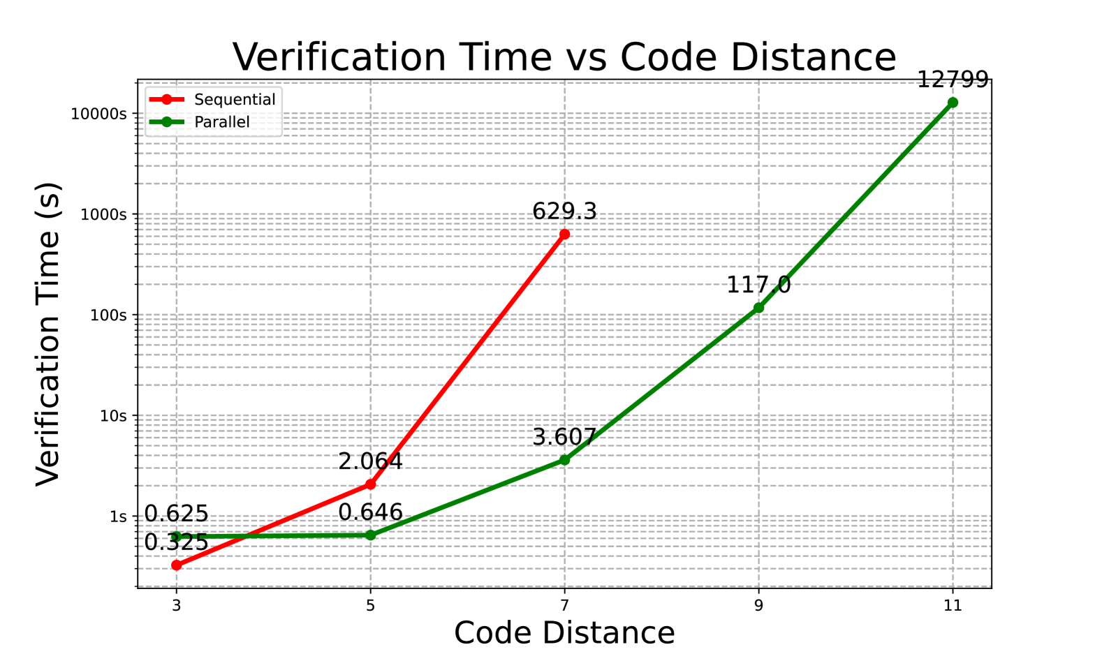
Figure 4. Time consumed when verifying surface code in sequential/parallel.

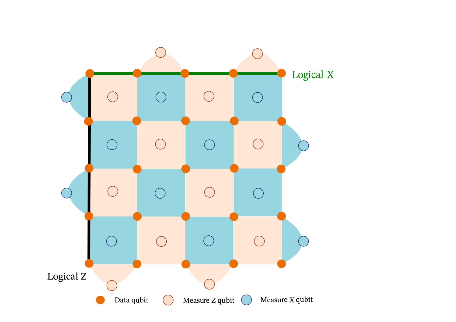
Figure 5. Scheme of a rotated surface code with $d=5$. Each coloured tile associated with the measure qubit in the center is a stabilizer (Flesh: Z check, Indigo: X check).

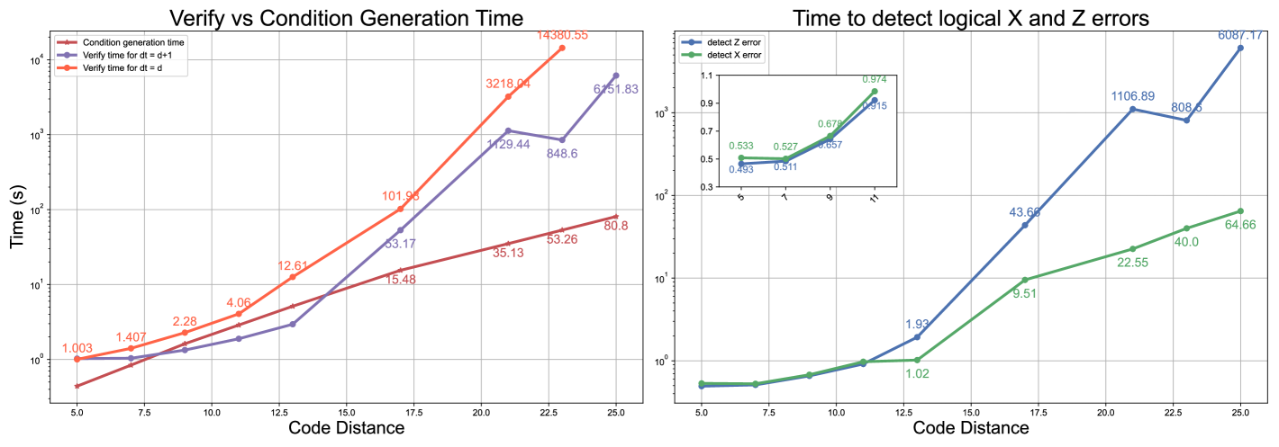
Figure 6. Time consumed when verifying precise detection properties on surface code with distance $d$.

Results

Accurate Decoding and Correction: Figure 5 illustrates the total runtime required to verify the error conditions for accurate decoding and correction, employing both sequential and parallel methods. The figure indicates that while both approaches produce correct results, our parallel strategy significantly improves the efficiency of the verification process. In contrast, the sequential method exceeds the maximum runtime of 24 hours at $d=9$; we have extended the threshold for solvable instances within the time limit to $d=11$.

Precise Detection of Errors: For a rotated surface code with distance $d$, we first set $d_{t}=d$ to verify that all error patterns with Hamming weight $<d$ can be detected by the stabilizer generators. Afterward, we set $d_{t}=d+1$ to detect error patterns that are undetectable by the stabilizer generators but cause logical errors. The results show that all trials with $d_{t}=d$ report unsat for Equation 15, and trials with $d_{t}=d+1$ report sat for Equation 15, providing evidence for the effectiveness of this functionality. The results indicate that, without prior knowledge of the minimum weight, this tool can identify and output the minimum weight undetectable error. In Figure 6 we illustrate the relationship between the time required for verifying error conditions of precise detection of errors and the code distance.

7.3. Verify correctness with user-provided errors

Constrained by the exponential growth of problem size, verifying general properties limits the size of QEC codes that can be analyzed. Therefore, we allow users to autonomously impose constraints on errors and verify the correctness of the QEC code under the specified constraints. We aim for the enhanced tool, after the implementation of these constraints, to increase the size of verifiable codes. Users have the flexibility to choose the generated constraints or derive them from experimental data, as long as they can be encoded into logical formulas supported by SMT solvers. The additional constraints will also help prune the solution space by eliminating infeasible enumeration paths during parallel solving.

Results

We briefly analyze the experimental data (Acharya et al., 2023, 2024) and observe that the error detection probabilities of stabilizer generators tend to be uniformly distributed. Moreover, among the physical qubits in the code, there are always several qubits that exhibit higher intrinsic single-qubit gate error rates. Based on these observations, we primarily consider two types of constraints and evaluate their effects in our experiment. For a rotated surface code with distance $d$, the explicit constraints are as follows:

• Locality: Errors occur within a set containing $\frac{d^{2}-1}{2}$ randomly chosen qubits. The other qubits are set to be error-free.

• Discreteness: Uniformly divide the total $d^{2}$ qubits into $d$ segments, within each segment of $d$ qubits there exists no more than one error.

The other experimental settings are the same as those in the first experiment.

In Figure 8 we illustrate the experimental results of verification with user-provided constraints. We separately assessed the results and the time consumed for verification with the locality constraint, the discreteness constraint, and both combined. We will take the average time for five runs for locality constraints since the locations of errors are randomly chosen. Obviously both constraints contribute to the improvement of efficiency, yet yield limited improvements if only one of them is imposed; When the constraints are imposed simultaneously, we can verify $d=19$ surface code which have $361$ qubits within $\sim 100$ minutes.

Comparison with Stim (Gidney, 2021)

Stim is currently the most widely used and state-of-the-art stabilizer circuit simulator that provides fast performance in sampling and testing large-scale QEC codes. However, simply using Stim in sampling or testing does not provide a complete check for QEC codes, as it will require a large number of samples. For example, we can verify a $d=19$ surface code with $361$ qubits in the presence of both constraints, which, require testing on $\sum_{i=0}^{18}\binom{18}{i}(18)^{i}=19^{18}\approx 2^{76}$ sample that is beyond the testing scope.

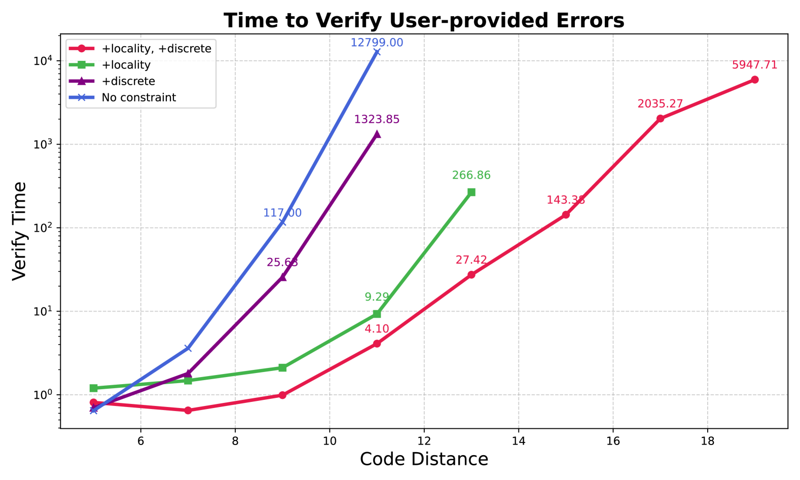
Figure 7. Time consumed to verify the correctness of surface code with distance range from $5$ to $19$.

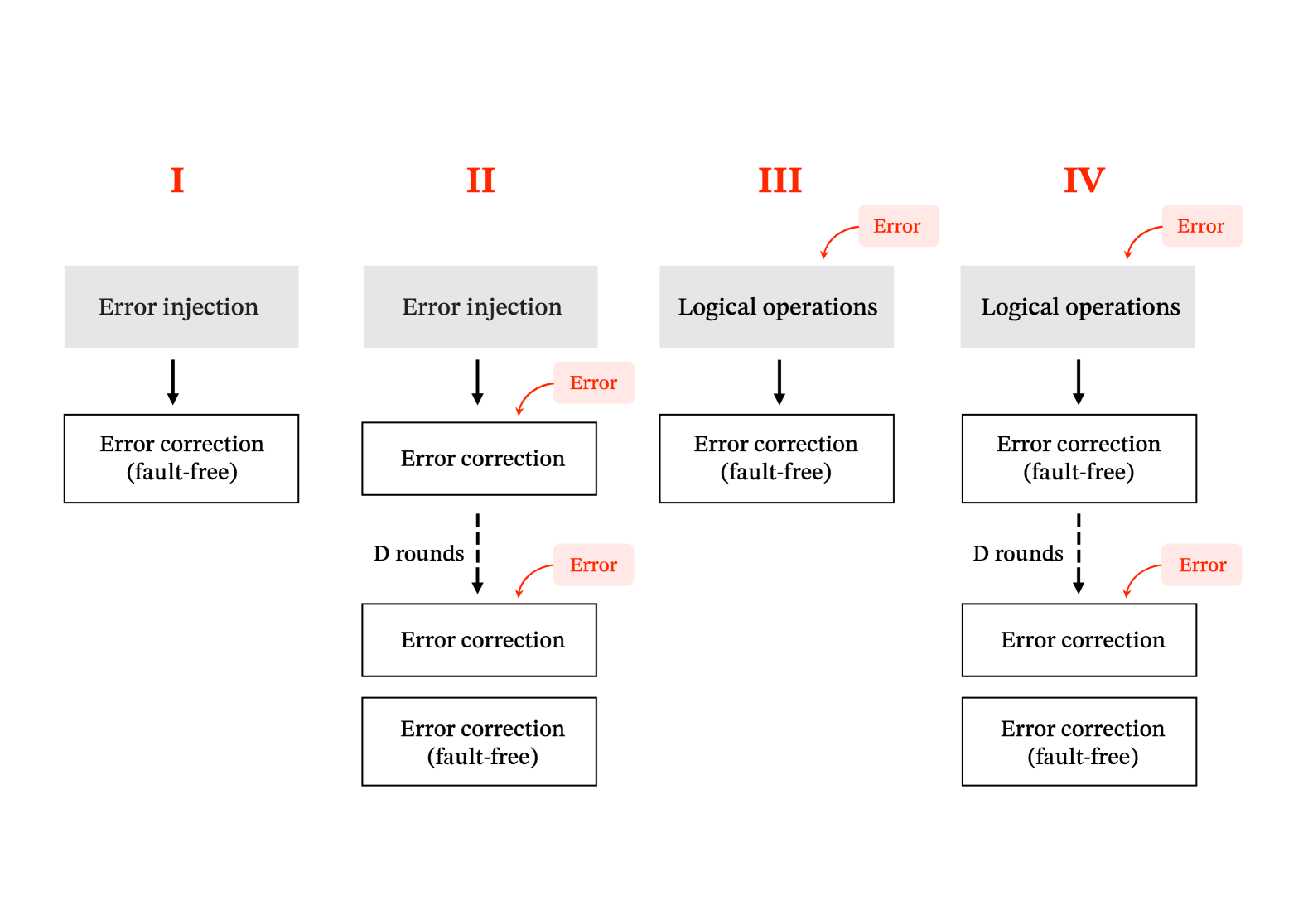
Figure 8. Realistic fault-tolerant scenarios that are supported for verification.

7.4. Towards fault-tolerant implementation of operations in quantum hardware

We are interested in whether our tool has the capability to verify the correctness of fault-tolerant implementations for certain logical operations or measurements. In Figure 8 we conclude the realistic fault-tolerant computation scenarios our tools support. In particular, we write down the programs of two examples encoded by Steane code and verify the correctness formula in our tool. The examples are stated as follows:

1. A fault-tolerant logical GHZ state preparation.

2. An error from the previous cycle remains uncorrected and got propagated through a logical CNOT gate.

We provide the programs used in the experiment in Figure 10 and Figure 10. The program Steane$(E)_{i}$ denotes an error correction process over $i^{\rm{th}}$ logical qubit.

$$\mathbf{for}\ i\in 8\cdots 14\ \mathbf{do}\ q_{i}\,*\!\!=H\ \mathbf{end}\ \fatsemi$$

$$\mathbf{for}\ i\in 1\cdots 3\ \mathbf{do}\ \textbf{Steane}(E)_{i}\ \mathbf{end}\ \fatsemi$$

$$\mathbf{for}\ i\in 8\cdots 14\ \mathbf{do}\ q_{i},q_{i-7}\,*\!\!=CNOT\ \mathbf{end}\ \fatsemi$$

$$\mathbf{for}\ i\in 1\cdots 7\ \mathbf{do}\ q_{i},q_{i+7}\,*\!\!=CNOT\ \mathbf{end}\ \fatsemi$$

$$\mathbf{for}\ i\in 1\cdots 3\ \mathbf{do}\ \textbf{Steane}(E)_{i}\ \mathbf{end}$$

Figure 9. QEC for logical GHZ state preparation.

$$\mathbf{for}\ i\in 1\cdots 7\ \mathbf{do}\ [ep_{(i)}]q_{i}\,*\!\!=U\ \mathbf{end}\ \fatsemi$$

$$\mathbf{for}\ i\in 1\cdots 7\ \mathbf{do}\ q_{i},q_{i+7}\,*\!\!=CNOT\ \mathbf{end}\ \fatsemi$$

$$\mathbf{for}\ i\in 1\cdots 2\ \mathbf{do}\ \textbf{Steane}(E)_{i}\ \mathbf{end}$$

Figure 10. QEC for logical CNOT gate with propagated errors.

7.5. A benchmark for qubit stabilizer codes

We further provide a benchmark of 14 qubit stabilizer codes selected from the broader quantum error correction code family, as illustrated in Table 3. We require the selected codes to be qubit-based and have a well-formed parity-check matrix. For codes which lack an explicit parity-check matrix, we construct the stabilizer generators and logical operators based on their mathematical construction and verify the correctness of the implementations. For codes with odd distances, we verify the correctness of their program implementations in the context of accurate decoding and correction. However, some codes have even code distances, including examples such as the 3D $[[8,3,2]]$ color code (Kubica et al., 2015) and the Campbell-Howard code (Campbell and Howard, 2017), which are designed to implement non-Clifford gates like the $T$-gate or Toffoli gate with low gate counts. These codes have a distance of 2, allowing error correction solely through post-selection rather than decoding. In such cases, the correctness of the program implementations is ensured by verifying that the code can successfully detect any single-qubit Pauli error. We list these error-detection codes at the end of Table 3.

Table 3. A benchmark of qubit stabilizer codes with logical-free scenario ($EMC$) considered in Table 4. We report their parameters $[[n,k,d]]$ and the properties we verified with the time spent. Parameters with variables indicate that this code has a scalable construction. If exact $d$ is unknown, we provide an estimation given by our tool in the bracket.

Target: Accurate Correction
Code Name	Parameters	Verify time(s)
Steane code (Steane, 1996a)	$[[7,1,3]]$	0.095
Surface code (Dennis et al., 2002) ($d=11$)	$[[d^{2},1,d]]$	12799
Six-qubit code (Calderbank et al., 1997)	$[[6,1,3]]$	0.252
Quantum dodecacode (Calderbank et al., 1997)	$[[11,1,5]]$	0.587
Reed-Muller code (Steane, 1996b) ($r=8$)	$[[2^{r}-1,1,3]]$	1868.56
XZZX surface code (Bonilla Ataides et al., 2021) ($d_{x}=9,d_{z}=11$)	$[[d_{x}\times d_{z},1,\min(d_{x},d_{z})]]$	1067.16
Goettsman code  (Gottesman, 1997) ($r=8$)	$[[2^{r},2^{r}-r-2,3]]$	1451.67
Honeycomb code (Landahl et al., 2011) ($d=5$)	$[[19,1,5]]$	1.55
Target: Detection
Tanner Code I (Leverrier and Zémor, 2022)	$[[343,31,$ $d\geq 4$]]	$7086.36$
Tanner Code II (Leverrier and Zémor, 2022)	$[[125,53,4]]$	$1667.81$
Hypergraph Product (Tillich and Zémor, 2014; Kovalev and Pryadko, 2012; Breuckmann and Eberhardt, 2021)	$[[98,18,4]]$	289.37
Error-Detection codes
3D basic color code (Kubica et al., 2015) ($d_{z}=2$)	$[[8,3,2]]$	2.88
Triorthogonal code (Bravyi and Haah, 2012) $(k=$$64$)	$[[3k+8,k,$ $d_{x}=6,d_{z}=2$]]	$144.94$
Carbon code (Grassl and Roetteler, 2013)	$[[12,2,4]]$	4.80
Campbell-Howard code (Campbell and Howard, 2017) ($k=2$)	$[[6k+2,3k,2]]$	3.05

8. Related Work

In addition to the works compared in Section 1, we briefly outline verification techniques for quantum programs and other works that may be used to check QEC programs.

Formal verification with program logic

Program logic, as a well-explored formal verification technique, plays a crucial role in the verification of quantum programs. Over the past decades, numerous studies have focused on developing Hoare-like logic frameworks for quantum programs (Baltag and Smets, 2004; Brunet and Jorrand, 2004; Chadha et al., 2006; Feng et al., 2007; Kakutani, 2009). Assertion Logic. (Wu et al., 2021; Rand et al., 2021a, b) began utilizing stabilizers as atomic propositions. (Unruh, 2019a) proposed a hybrid quantum logic in which classical variables are embedded as special quantum variables. Although slightly different, this approach is essentially isomorphic to our interpretation of logical connectives. Program Logic. Several works have established sound and relatively complete (hybrid) quantum Hoare logics, both satisfaction-based (Ying, 2012; Feng and Ying, 2021) and projection-based (Zhou et al., 2019). However, these works did not introduce (countable) assertion syntax, meaning their completeness proofs do not account for the expressiveness of the weakest (liberal) preconditions. (Wu et al., 2021; Wu, 2024; Sundaram et al., 2022) focus on reasoning about stabilizers and QEC code, with our substitution rules for unitary statements drawing inspiration from their work. Program logic in the verification of QEC codes and fault-tolerant computing. Quantum relational logic (Unruh, 2019b; Li and Unruh, 2021; Barthe et al., 2019) is designed for reasoning about relationships, making it well-suited for verifying functional correctness by reasoning equivalence between ideal programs and programs with errors. Quantum separation logic (Le et al., 2022; Zhou et al., 2021; Li et al., 2024; Hietala et al., 2022), through the application of separating conjunctions, enables local and modular reasoning about large-scale programs, which is highly beneficial for verifying large-scale fault-tolerant computing. Abstract interpretation (Yu and Palsberg, 2021) uses a set of local projections to characterize properties of global states, thereby breaking through the exponential barrier. It is worth investigating whether local projections remain effective for QEC codes.

Symbolic techniques for quantum computation

General quantum program testing and debugging methods face the challenge of excessive test cases when dealing with QEC programs, which makes them inefficient. Symbolic techniques have been introduced into quantum computing to address this issue (Carette et al., 2023; Bauer-Marquart et al., 2023; Tao et al., 2022; Chen et al., 2023; Huang et al., 2021; Fang and Ying, 2024). Some of these works aim to speed up the simulation process without providing complete verification of quantum programs, while others are designed for quantum circuits and do not support the control flows required in QEC programs. The only approach capable of handling large-scale QEC programs is the recent work that proposed symbolic stabilizers (Fang and Ying, 2024). However, this framework is primarily designed to detect bugs in the error correction process that do not involve logical operations and do not support non-Clifford gates.

Mechanized approach for quantum programming

The mechanized approach offers significant advantages in terms of reliability and automation, leading to the development of several quantum program verification tools in recent years (see recent reviews (Chareton et al., 2023; Lewis et al., 2023)). Our focus is primarily on tools that are suitable for writing and reasoning about quantum error correction (QEC) code at the circuit level. Matrix-based approaches. $\mathcal{Q}$wire (Paykin et al., 2017; Rand et al., 2017) and SQIR (Hietala et al., 2021) formalize circuit-like programming languages and low-level languages for intermediate representation, utilizing a density matrix representation of quantum states. These approaches have been extended to develop verified compilers (Rand et al., 2018) and optimizers (Hietala et al., 2021). Graphical-based approaches. (Lehmann et al., 2022, 2023; Shah et al., 2024), provide a certified formalization of the ZX-calculus (Coecke and Duncan, 2011; Kissinger and van de Wetering, 2019), which is effective for verifying quantum circuits through a flexible graphical structure. Automated verification. Qbricks (Chareton et al., 2021) offers a highly automated verification framework based on the Why3 (Bobot et al., 2011) prover for circuit-building quantum programs, employing path-sum representations of quantum states (Amy, 2018). Theory formalization. Ongoing libraries are dedicated to the formalization of quantum computation theories, such as QuantumLib (Zweifler et al., 2022), Isabelle Marries Dirac (IMD) (Bordg et al., 2021, 2020), and CoqQ (Zhou et al., 2023). QuantumLib is built upon the Coq proof assistant and utilizes the Coq standard library as its mathematical foundation. IMD is implemented in Isabelle/HOL, focusing on quantum information theory and quantum algorithms. CoqQ is written in Coq and provides comprehensive mathematical theories for quantum computing based on the Mathcomp library (Mahboubi and Tassi, 2022; The MathComp Analysis Development Team, 2024). Among these, CoqQ has already formalized extensive theories of subspaces, making it the most suitable choice for our formalization of program logic.

Functionalities of verification tools for QEC programs

Besides the comparison of theoretical work on program logic and other verification methods, we also compare the functionalities of our tool Veri-QEC with those of other verification tools for QEC programs. We summarize the functionalities of the tools in Table 4. VERITA (Wu et al., 2021; Wu, 2024) adopts a logic-based approach to verify the implementation of logical operations with fixed errors. QuantumSE (Fang and Ying, 2024) is tailored for efficiently reporting bugs in QEC programs and shows potential in handling logical Clifford operations. Stim (Gidney, 2021) employs a simulation-based approach, offering robust performance across diverse fault-tolerant scenarios but limited to fixed errors. Our tool Veri-QEC is designed for both general verification and partial verification under user-provided constraints, supporting all aforementioned scenarios.

Table 4. Comparison of scenarios and functionalities between Veri-QEC and other tools. For scenarios, we denote $\bar{L}$ for logical gate implementation, $E$ for error injection, $M$ for measurement (error detection), $C$ ($C_{E}$) for error correction (with error injection). We further identify three functionalities, C for general verification of correctness, R for reporting bugs, , and F for fixed errors, that evaluated by $\blacktriangle$ if implemented, $\circ$ if potentially supported but not yet implemented and $-$ if cannot handle or beyond design. N.A indicates that F is unavailable in the error-free scenario.

	Veri-QEC			VERITA (Wu, 2024; Wu et al., 2021)			QuantumSE (Fang and Ying, 2024)			Stim (Gidney, 2021)
Functionality	C	R	F	C	R	F	C	R	F	C	R	F
error-free ($\bar{L}$)	$\blacktriangle$	$\circ$	N.A	$\blacktriangle$	$\circ$	N.A	$\circ$	$\circ$	N.A	$\circ$	$\circ$	N.A
logical-free ($EMC$)	$\blacktriangle$	$\circ$	$\circ$	$-$	$-$	$\blacktriangle$	$\blacktriangle$	$\blacktriangle$	$\circ$	$-$	$-$	$\blacktriangle$
error in correction step ($\bar{L}MC_{E}$)	$\blacktriangle$	$\circ$	$\circ$	$-$	$-$	$\circ$	$\blacktriangle$	$\blacktriangle$	$\circ$	$-$	$-$	$\blacktriangle$
one cycle ($E\bar{L}EMC$)	$\blacktriangle$	$\circ$	$\circ$	$-$	$-$	$\blacktriangle$	$\blacktriangle$	$\blacktriangle$	$\circ$	$-$	$-$	$\blacktriangle$
multi cycles ($E\bar{L}EMCE\bar{L}EMC\cdots$)	$\blacktriangle$	$\circ$	$\circ$	$-$	$-$	$\blacktriangle$	$\circ$	$\circ$	$\circ$	$-$	$-$	$\blacktriangle$

9. Discussion and future works

In this paper, we propose an efficient verification framework for QEC programs, within which we define the assertion logic along with program logic and establish a sound proof system. We further develop an efficient method to handle verification conditions of QEC programs. We implement our QEC verifiers at two levels: a verified QEC verifier and a Python-based automated QEC verifier.

Our work still has some limitations. First of all, the gate set we adopt in the programming language is restricted, and the current projection-based logic is unable to reason about probabilities. Last but not least, while our proof system is sound, its completeness- especially for programs with loops- remains an open question.

Given the existing limitations, some potential directions for future advancements include:

1. Address the completeness issue of the proof system. We are able to prove the (relative) completeness of our proof system for finite QEC programs without infinite loops. However, it is still open whether the proof system is complete for programs with while-loops. This issue is indeed related to the next one.

2. Extend the gate set to enhance the expressivity of program logic. The Clifford + T gate set we use in the current program logic is universal but still restricted in practical applications. It is desirable to extend the syntax of factors and assertions for the gate sets beyond Clifford + T.

3. Generalize the logic to satisfaction-based approach. Since any Hermitian operator can be written as linear combinations of Pauli expressions, our logic has the potential to incorporate so-called satisfaction-based approach with Hermitian operators as quantum predicates, which helps to reason about the success probabilities of quantum QEC programs.

4. Explore approaches to implementing an automatic verified verifier. The last topic is to explore tools like $F^{*}$ (Swamy et al., 2016; Martínez et al., 2019), a proof-oriented programming language based on SMT, for incorporating the formally verified verifier and the automatic verifier described in this paper into a single unified solution.

Acknowledgement

We thank Bonan Su and Huiping Lin for kind discussion, and we thank anonymous referees for helpful comments and suggestions. This research was supported by the National Key R&D Program of China under Grant No. 2023YFA1009403.

Data Availability Statement

Our code is available at https://github.com/Chesterhuang1999/Veri-qec.

Appendix A Supplementary materials for Section 3 and Section 4

Here we provide technical details for Section 3 regarding the assertion logic in Section 3. All lemmas and theorems are proved in our Coq implementation based on CoqQ (Zhou et al., 2023).

A.1. A Syntax of Basic Expression

We first claim the expressivity of $SExp$ and $PExp$ discussed in the main context.

Proposition A.1 (Expressivity of $SExp$ and $PExp$).

Any constant $s\in\mathbb{Z}[\frac{1}{\sqrt{2}}]$ is expressible in $SExp$. Any constant $W$ belonging to the Pauli group over qubits $1,\cdots,n$ is expressible in $PExp$.

We further specify the boolean expressions $BExp$ and integer expressions $IExp$ for Veri-QEC  as:

$$IExp:\quad a\Coloneqq\ n\in\mathbb{N}\mid x\mid-a\mid a_{1}+a_{2}\mid a_{1}\times a_{2}$$

$$BExp:\quad b\Coloneqq\ \mathbf{true}\mid\mathbf{false}\mid x\mid a_{1}==a_{2}\mid a_{1}\leq a_{2}$$

$$\mid\neg b\mid b_{1}\wedge b_{2}\mid b_{1}\vee b_{2}\mid b_{1}\rightarrow b_{1}.$$

Here, $n$ are constant natural numbers, $x$ appears in $IExp$ and $BExp$ are program variables of type integer and bool, respectively. There exists type coercion between $BExp$ and $IExp$: boolean value $\mathbf{true}$ and $\mathbf{false}$ are identified with 1 and 0, respectively. Their semantics $\llbracket a\rrbracket_{m}$ and $\llbracket b\rrbracket_{m}$ are defined conventionally as a mapping from classical state $m\in\mathtt{CMem}$ to integers and bools:

$$\llbracket n\rrbracket_{m}\triangleq n,\quad\llbracket x\rrbracket_{m}\triangleq m(x),\quad\llbracket-a\rrbracket_{m}\triangleq-\llbracket a\rrbracket_{m},$$

$$\llbracket a_{1}+a_{2}\rrbracket_{m}\triangleq\llbracket a_{1}\rrbracket_{m}+\llbracket a_{2}\rrbracket_{m},\quad\llbracket a_{1}\times a_{2}\rrbracket_{m}\triangleq\llbracket a_{1}\rrbracket_{m}\times\llbracket a_{2}\rrbracket_{m},$$

$$\llbracket\mathbf{true}\rrbracket_{m}\triangleq\mathbf{true},\quad\llbracket\mathbf{false}\rrbracket_{m}\triangleq\mathbf{false},\quad\llbracket x\rrbracket_{m}\triangleq m(x),\quad$$

$$\llbracket a_{1}==a_{2}\rrbracket_{m}\triangleq\llbracket a_{1}\rrbracket_{m}==\llbracket a_{2}\rrbracket_{m},\quad\llbracket a_{1}\leq a_{2}\rrbracket_{m}\triangleq\llbracket a_{1}\rrbracket_{m}\leq\llbracket a_{2}\rrbracket_{m},$$

$$\llbracket\neg b\rrbracket_{m}\triangleq\neg\llbracket b\rrbracket_{m},\quad\llbracket b_{1}\wedge b_{2}\rrbracket_{m}\triangleq\llbracket b_{1}\rrbracket_{m}\wedge\llbracket b_{2}\rrbracket_{m},$$

$$\llbracket b_{1}\vee b_{2}\rrbracket_{m}\triangleq\llbracket b_{1}\rrbracket_{m}\vee\llbracket b_{2}\rrbracket_{m},\quad\llbracket b_{1}\rightarrow b_{2}\rrbracket_{m}\triangleq\llbracket b_{1}\rrbracket_{m}\rightarrow\llbracket b_{2}\rrbracket_{m}.$$

A.2. The Pauli expression is closed under basic unitary transformation

To provide proof rules for the unitary transformation of single-qubit gates $U_{1}\in\{X,Y,Z,H,S,T\}$ and two-qubit gates $U_{2}\in\{CNOT,CZ,iSWAP\}$ for the program logic, we need first examine the properties that, for any $P\in PExp$, is $U_{1i}^{\dagger}\llbracket P\rrbracket_{m}U_{1i}$ and $U_{2ij}^{\dagger}\llbracket P\rrbracket_{m}U_{2ij}$ expressible in $PExp$? Here, we give an affirmative result stated below:

Theorem A.2 (Theorem 3.1).

For any Pauli expression $P$ defined in Eqn. 4 and single-qubit gate $U_{1}$ acts on $q_{i}$ or two-qubit gate $U_{2}$ acts on $q_{i}q_{j}$, their exists another Pauli expression $Q\in PExp$, such that for all $m\in\mathtt{CMem}$:

$$\llbracket Q\rrbracket_{m}=U_{1i}^{\dagger}\llbracket P\rrbracket_{m}U_{1i},\quad\mbox{or},\quad\llbracket Q\rrbracket=U_{2ij}^{\dagger}\llbracket P\rrbracket_{m}U_{2ij}.$$

Proof.

We prove it by induction on the structure of $PExp$. The proofs of all gates are similar, we here only present the case for $T$ gate and $CNOT$ gate.

$\bullet$ ($T$ gate). Define the substitution of any $P\in PExp$ as

$$P^{\prime}\triangleq P\big{[}\frac{1}{\sqrt{2}}(X_{i}-Y_{i})/X_{i},\frac{1}{\sqrt{2}}(X_{i}+Y_{i})/Y_{i}\big{]},$$

where $i$ is the qubit $q_{i}$ the $T$ gate acts on, and $P[e_{1}/x_{1},e_{2}/x_{2},\cdots]$ are simultaneous substitution of constant constructor $x\in\{X_{r},Y_{r},Z_{r}\}$ with expression $e$ in $P$. We then show that $P^{\prime}$ is the desired $Q$.

Base case. For elementary expression $P\equiv p_{r}$, if $r\neq i$, then:

$$T^{\dagger}_{q_{i}}\llbracket p_{r}\rrbracket_{m}T_{q_{i}}=I_{1}\otimes\cdots\otimes T^{\dagger}_{i}I_{i}T_{i}\otimes\cdots\otimes p_{r}\otimes\cdots I_{n}=I_{1}\otimes\cdots\otimes I_{i}\otimes\cdots\otimes p_{r}\otimes\cdots I_{n}=\llbracket p_{r}\rrbracket_{m}=\llbracket p_{r}^{\prime}\rrbracket_{m},$$

i.e., we do not need to change $p_{r}$ in the case of $r\neq i$. On the other hand, note that:

$$T^{\dagger}XT=\frac{1}{\sqrt{2}}(X-Y),\quad T^{\dagger}YT=\frac{1}{\sqrt{2}}(X+Y),\quad T^{\dagger}ZT=Z,$$

so we obtain:

$$T^{\dagger}_{q_{i}}\llbracket X_{i}\rrbracket_{m}T_{q_{i}}=I_{1}\otimes\cdots\otimes\frac{1}{\sqrt{2}}(X_{i}-Y_{i})\otimes\cdots\otimes I_{n}=\llbracket\frac{1}{\sqrt{2}}(X_{i}-Y_{i})\rrbracket_{m}=\llbracket X_{i}^{\prime}\rrbracket_{m}$$

$$T^{\dagger}_{q_{i}}\llbracket Y_{i}\rrbracket_{m}T_{q_{i}}=\llbracket\frac{1}{\sqrt{2}}(X_{i}+Y_{i})\rrbracket_{m}=\llbracket Y_{i}^{\prime}\rrbracket_{m},\qquad T^{\dagger}_{q_{i}}\llbracket Z_{i}\rrbracket_{m}T_{q_{i}}=\llbracket Z_{i}\rrbracket_{m}=\llbracket Z_{i}^{\prime}\rrbracket_{m}.$$

Induction step. $P\equiv sP$. Note that

$$T^{\dagger}_{q_{i}}\llbracket sP\rrbracket_{m}T_{q_{i}}=T^{\dagger}_{q_{i}}\llbracket s\rrbracket_{m}\llbracket P\rrbracket_{m}T_{q_{i}}=\llbracket s\rrbracket_{m}(T^{\dagger}_{q_{i}}\llbracket P\rrbracket_{m}T_{q_{i}})=\llbracket s\rrbracket_{m}\llbracket P^{\prime}\rrbracket_{m}=\llbracket sP^{\prime}\rrbracket_{m}=\llbracket(sP)^{\prime}\rrbracket_{m}.$$

$P\equiv P_{1}+P_{2}$. Observe that

$$T^{\dagger}_{q_{i}}\llbracket P_{1}+P_{2}\rrbracket_{m}T_{q_{i}} =T^{\dagger}_{q_{i}}(\llbracket P_{1}\rrbracket_{m}+\llbracket P_{1}\rrbracket_{m})T_{q_{i}}=T^{\dagger}_{q_{i}}\llbracket P_{1}\rrbracket_{m}T_{q_{i}}+T^{\dagger}_{q_{i}}\llbracket P_{1}\rrbracket_{m}T_{q_{i}}$$

$$=\llbracket P_{1}^{\prime}\rrbracket_{m}+\llbracket P_{2}^{\prime}\rrbracket_{m}=\llbracket P_{1}^{\prime}+P_{2}^{\prime}\rrbracket_{m}=\llbracket(P_{1}+P_{2})^{\prime}\rrbracket_{m}.$$

$P\equiv P_{1}P_{2}$. By noticing that $T^{\dagger}T=I$, we have:

$$T^{\dagger}_{q_{i}}\llbracket P_{1}P_{2}\rrbracket_{m}T_{q_{i}} =T^{\dagger}_{q_{i}}(\llbracket P_{1}\rrbracket_{m}\llbracket P_{2}\rrbracket_{m})T_{q_{i}}=(T^{\dagger}_{q_{i}}\llbracket P_{1}\rrbracket_{m}T_{q_{i}})(T^{\dagger}_{q_{i}}\llbracket P_{2}\rrbracket_{m}T_{q_{i}})$$

$$=\llbracket P_{1}^{\prime}\rrbracket_{m}\llbracket P_{2}^{\prime}\rrbracket_{m}=\llbracket P_{1}^{\prime}P_{2}^{\prime}\rrbracket_{m}=\llbracket(P_{1}P_{2})^{\prime}\rrbracket_{m}.$$

$\bullet$ ($CNOT$ gate). Define the substitution of any $P\in PExp$ as

$$P^{\prime}\triangleq P[X_{i}X_{j}/X_{i},Y_{i}X_{j}/Y_{i},Z_{i}Y_{j}/Y_{j},Z_{i}Z_{j}/Z_{j}],$$

and $P^{\prime}$ is the desired $Q$. The induction step is the same as of $T$. For the base case, we shall analyze the case that $r=i$ or $r=j$ or $r\neq i,j$. First, we observe the following facts:

$$CNOT_{ij}(X_{i}\otimes I_{j})CNOT_{ij}=X_{i}\otimes X_{j},\quad CNOT_{ij}(I_{i}\otimes X_{j})CNOT_{ij}=I_{i}\otimes X_{j}$$

$$CNOT_{ij}(Y_{i}\otimes I_{j})CNOT_{ij}=Y_{i}\otimes X_{j},\quad CNOT_{ij}(I_{i}\otimes Y_{j})CNOT_{ij}=Z_{i}\otimes Y_{j}$$

$$CNOT_{ij}(Z_{i}\otimes I_{j})CNOT_{ij}=Z_{i}\otimes I_{j},\quad CNOT_{ij}(I_{i}\otimes Z_{j})CNOT_{ij}=Z_{i}\otimes Z_{j}.$$

For $r\neq i,j$, $CNOT_{ij}^{\dagger}\llbracket p_{r}\rrbracket_{m}CNOT_{ij}=\llbracket p_{r}\rrbracket_{m}=\llbracket p_{r}^{\prime}\rrbracket_{m}$.

If $r=i$, then for example $X_{i}$, we calculate :

$$CNOT_{ij}\llbracket X_{i}\rrbracket_{m}CNOT_{ij} =\bigotimes_{k\neq i,j}I_{k}\otimes(CNOT_{ij}(X_{i}\otimes I_{j})CNOT_{ij})=\bigotimes_{k\neq i,j}I_{k}\otimes X_{i}\otimes X_{j}$$

$$=\big{(}\bigotimes_{k\neq i}I_{k}\otimes X_{i}\big{)}\big{(}\bigotimes_{k\neq j}I_{k}\otimes X_{j}\big{)}=\llbracket X_{i}X_{j}\rrbracket_{m}=\llbracket X_{i}^{\prime}\rrbracket_{m}.$$

The rest case $Y_{i},Z_{i}$ and $X_{j},Y_{j},Z_{j}$ are similar.

∎

A.3. A Brief Review of Hilbert Subspace

We first briefly review the basic operations regarding subspaces of Hilbert space $\mathcal{H}$. Since we focus on the finite-dimensional case, any subspace of $\mathcal{H}$ is always closed.

• (span) Given a set of states $S\subseteq\mathcal{H}$, its span $\operatorname{span}\{S\}\in\mathcal{S}(\mathcal{H})$ is defined by

  $$\operatorname{span}\{S\}=\Big{\{}\sum_{i\in I}\lambda_{i}|\phi_{i}\rangle:I\mbox{ is a finite index set, }\lambda_{i}\in\mathbb{C}\mbox{, and }|\phi_{i}\rangle\in S\Big{\}}.$$

• (kernel) Given a linear operator $A$ on $\mathcal{H}$, its kernel $\ker(A)\in\mathcal{S}(\mathcal{H})$ is defined by

  $$\ker(A)=\{|\psi\rangle\in\mathcal{H}:A|\psi\rangle=0\}.$$

• (+1-eigenspace) Given a linear operator $A$ on $\mathcal{H}$, its +1-eigenspace $E_{1}(A)\in\mathcal{S}(\mathcal{H})$ is defined by

  $$E_{1}(A)=\{|\psi\rangle\in\mathcal{H}:A|\psi\rangle=|\psi\rangle\}.$$

• (complement, or orthocomplement) For a given subspace $S\in\mathcal{S}(\mathcal{H})$, its orthocomplement $S^{\bot}\in\mathcal{S}(\mathcal{H})$ is defined by

  $$S^{\bot}=\{|\psi\rangle:\forall\ |\phi\rangle\in S,\ |\psi\rangle\perp|\phi\rangle\}.$$

  Orthocomplement is involutive, i.e., $S^{\bot\bot}=S$.

• (support) Given a linear operator $A$ on $\mathcal{H}$, its support $\mathrm{supp}(A)\in\mathcal{S}(\mathcal{H})$ is defined as the orthocomplement of its kernel, i.e., $\mathrm{supp}(A)=\ker(A)^{\bot}$. Support is idempotent, i.e., $\operatorname{supp}(\operatorname{supp}(A))=\operatorname{supp}(A)$.

• (meet, or intersection, or disjunction) Given two subspaces $S,T\in\mathcal{S}(\mathcal{H})$, their meet $S\wedge T\in\mathcal{S}(\mathcal{H})$ is defined as the intersection:

  $$S\wedge T=S\cap T\equiv\{|\phi\rangle:|\phi\rangle\in S\mbox{ and }|\phi\rangle\in T\}.$$

• (join, or conjunction, or span of the union) Given two subspaces $S,T\in\mathcal{S}(\mathcal{H})$, their join $S\vee T\in\mathcal{S}(\mathcal{H})$ is defined as:

  $$S\vee T=\operatorname{span}\{S\cup T\}.$$

  It holds that: $(S\vee T)^{\bot}=S^{\bot}\wedge T^{\bot}$ and $(S\wedge T)^{\bot}=S^{\bot}\vee T^{\bot}$. Generally, there is no distributivity of $\vee$ and $\wedge$.

• (commute) Given two subspaces $S,T\in\mathcal{S}(\mathcal{H})$, we say $S$ commutes with $T$, written $S\mathtt{C}T$, if $S=(S\wedge T)\vee(S\wedge T^{\bot}).$ Commutativity plays an essential role in reasoning about Hilbert space. Some properties include:

  $$S\mathtt{C}T\mbox{ iff }T\mathtt{C}S,\quad S\mathtt{C}S,\quad S\subseteq T\mbox{ implies }S\mathtt{C}T,\quad S\mathtt{C}T\mbox{ implies }S\mathtt{C}T^{\bot}.$$

  Distributivity of meet and join holds when commutativity is assumed: if two of $S\mathtt{C}T_{1},S\mathtt{C}T_{2},T_{1}\mathtt{C}T_{2}$ hold, then:

  $$S\wedge(T_{1}\vee T_{2})=(S\wedge T_{1})\vee(S\wedge T_{2}),\quad S\vee(T_{1}\wedge T_{2})=(S\vee T_{1})\wedge(S\vee T_{2}).$$

• (Sasaki implication) Given two subspaces $S,T\in\mathcal{S}(\mathcal{H})$, the Sasaki implication $S\rightsquigarrow T\in\mathcal{S}(\mathcal{H})$ is defined by

  $$S\rightsquigarrow T=S^{\bot}\vee(S\wedge T).$$

  Sasaki implication is viewed as an extension of classical implication in quantum logic since it satisfies Birkhoff-von Neumann requirement: $S\rightsquigarrow T=I$ if and only if $S\subseteq T$, and the compatible import-export law: if $S$ commutes with $T$, then for any $W$, $S\wedge T\subseteq W$ if and only if $S\subseteq W\rightsquigarrow T$.

• (Sasaki projection) Given two subspaces $S,T\in\mathcal{S}(\mathcal{H})$, the Sasaki projection $S\doublecap T\in\mathcal{S}(\mathcal{H})$ is defined by

  $$S\doublecap T=S\wedge(S^{\bot}\vee T).$$

  Sasaki projection is a “dual” of implication, i.e., $(S\doublecap T)^{\bot}=S\rightsquigarrow T^{\bot}$, $(S\rightsquigarrow T)^{\bot}=S\doublecap T^{\bot}$. It preserves order for the second parameter, i.e., $T_{1}\subseteq T_{2}$ implies $S\doublecap T_{1}\subseteq S\doublecap T_{2}$. $\operatorname{supp}(P_{S}AP_{S})=P_{S}\doublecap\operatorname{supp}(A)$ which appears useful for reasoning about measurement (Feng et al., 2023).

A.4. A Hilbert-style Proof System of Assertion Logic

The proof system presented in Fig. A.4 is sound for quantum logic, and thus is also sound for our assertions, as its semantics is a point-wise lifting of quantum logic. We say two assertions $A,B$ commute, written $A\mathtt{C}B$, if for all $m$, $\llbracket A\rrbracket_{m}\mathtt{C}\llbracket B\rrbracket_{m}$.

$$1.\ \inferrule{} 2.\ \inferrule{}{A\vdash A} 3.\ \inferrule{}{A\vdash\top} 4.\ \inferrule{}{\bot\vdash A}$$

$$5.\ \inferrule{\Gamma\vdash A\quad\Gamma\vdash B}{\Gamma\vdash A\wedge B} 6.\ \inferrule{\Gamma\vdash A_{1}\wedge A_{2}}{\Gamma\vdash A_{i}} 7.\ \inferrule{A\vdash B}{\Gamma\wedge A\vdash B} 8.\ \inferrule{\Gamma\vdash A\quad\Gamma^{\prime}\vdash A}{\Gamma\vee\Gamma^{\prime}\vdash A}$$

$$9.\ \inferrule{\Gamma\vdash A_{i}}{\Gamma\vdash A_{1}\vee A_{2}} 10.\ \inferrule{A\vdash B\Rightarrow C\quad A\vdash B}{A\vdash C} 11.\ \inferrule{A\wedge B\vdash C\quad A\mathtt{C}B}{A\vdash B\Rightarrow C}$$

Figure 11. A Hilbert-style proof system for assertion logic.

We also provide two auxiliary laws to help simplify special Pauli expressions:

Proposition A.3.

For any $P,Q\in PExp$, the following laws are correct: $$\mathrm{i})\ P\wedge Q\mathrel{\reflectbox{{$\models$}}}\!\>\!\models P\wedge QP,\qquad\mathrm{ii})\ P\wedge-P\mathrel{\reflectbox{{$\models$}}}\!\>\!\models\mathbf{false}.$$

A.5. Denotational Semantics of QEC programs

Feng and Ying (2021) gives the induced denotational semantics of the classical-quantum program, the structural representation of each construct is as follows:

Proposition A.4 (c.f. (Feng and Ying, 2021)).

The denotational semantics for QEC programs enjoy the following structure representation:

1. $\llbracket\mathbf{skip}\rrbracket(m,\rho)=(m,\rho)$;

2. $\llbracket q_{i}\coloneq|0\rangle\rrbracket(m,\rho)=(m,\sum_{k=0,1}|0\rangle_{q_{i}}\langle k|\rho|k\rangle_{q_{i}}\langle 0|)$;

3. $\llbracket q_{i}\,*\!\!=U\rrbracket(m,\rho)=(m,U_{q_{i}}\rho U_{q_{i}}^{{\dagger}})$;

4. $\llbracket q_{i}q_{j}\,*\!\!=U\rrbracket(m,\rho)=(m,U_{q_{i,j}}\rho U_{q_{i,j}}^{{\dagger}})$;

5. $\llbracket x\coloneq e\rrbracket(m,\rho)=(m[\llbracket e\rrbracket_{m}/x],\rho)$;

6. $\llbracket S_{1}\fatsemi S_{2}\rrbracket(m,\rho)=\sum_{o\in\mathtt{CMem}}\llbracket S_{2}\rrbracket(o,\llbracket S_{1}\rrbracket(m,\rho)(o))$;

7. $\llbracket x\coloneq\mathbf{meas}[P]\rrbracket(m,\rho)=(m[0/x],\mathtt{P}_{\llbracket P\rrbracket_{m}}\rho\mathtt{P}_{\llbracket P\rrbracket_{m}})+(m[1/x],\mathtt{P}_{\llbracket P\rrbracket_{m}^{\bot}}\rho\mathtt{P}_{\llbracket P\rrbracket_{m}^{\bot}})$;

8. $\llbracket\mathbf{if}\ b\ \mathbf{then}\ S_{1}\ \mathbf{else}\ S_{0}\ \mathbf{end}\rrbracket(m,\rho)=\left\{\begin{aligned} &\llbracket S_{0}\rrbracket(m,\rho),\ b\equiv\mathbf{false}\\ &\llbracket S_{1}\rrbracket(m,\rho),\ b\equiv\mathbf{true}\end{aligned}\right.$;

9. $\llbracket\mathbf{while}\ b\ \mathbf{do}\ S\ \mathbf{end}\rrbracket(m,\rho)=\lim_{n}(\llbracket(\mathbf{while})^{n}\rrbracket(m,\rho)).$

Note that projection is Hermitian, so we omit ^† in (7). $(\mathbf{while})^{n}$ is the $n$-th syntactic approximation of $\mathbf{while}$, i.e., $(\mathbf{while})^{0}=\mathbf{abort}$, and $(\mathbf{while})^{(n+1)}=\mathbf{if}\ b\ \mathbf{then}\ S\fatsemi(\mathbf{while})^{n}\ \mathbf{else}\ \mathbf{skip}\ \mathbf{end}$. As mentioned, we do not lift the input state from singleton to the general classical-quantum state, (6) is thus slightly different from (Feng and Ying, 2021). In (9), as the sequence always converges, we simply write $\lim$ instead of the least upper bound in (Feng and Ying, 2021).

It is alternative to express denotational semantics as $\llbracket S\rrbracket^{\prime}:\mathtt{CMem}\rightarrow\mathtt{CMem}\rightarrow\mathcal{QO}(\mathcal{H})$; for given input and output classical state $m_{in}$ and $m_{out}$, the evolution of quantum system is described by quantum operation $\llbracket S\rrbracket^{\prime}_{m_{in},m_{out}}$, and $\llbracket S\rrbracket^{\prime}_{m_{in},m_{out}}(\rho)=\llbracket S\rrbracket(m_{in},\rho)(m_{out})$. Some structure representations of $\llbracket S\rrbracket^{\prime}$ are as follows:

1. $\llbracket\mathbf{skip}\rrbracket^{\prime}_{m,m}=\mathcal{I}$ and $\llbracket\mathbf{skip}\rrbracket^{\prime}_{m,m^{\prime}}=0$ if $m\neq m^{\prime}$;

2. $\llbracket q_{i}\coloneq|0\rangle\rrbracket^{\prime}_{m,m}(\rho)=\sum_{k=0,1}|0\rangle_{q_{i}}\langle k|\rho|k\rangle_{q_{i}}\langle 0|$ and $\llbracket q_{i}\coloneq|0\rangle\rrbracket^{\prime}_{m,m^{\prime}}=0$ if $m\neq m^{\prime}$;

3. $\llbracket q_{i}\,*\!\!=U\rrbracket^{\prime}_{m,m}(\rho)=U_{i}\rho U_{i}^{{\dagger}}$ and $\llbracket q_{i}\,*\!\!=U\rrbracket^{\prime}_{m,m^{\prime}}=0$ if $m\neq m^{\prime}$;

4. $\llbracket q_{i}q_{j}\,*\!\!=U\rrbracket^{\prime}_{m,m}(\rho)=U_{ij}\rho U_{ij}^{{\dagger}}$ and $\llbracket q_{i}q_{j}\,*\!\!=U\rrbracket^{\prime}_{m,m^{\prime}}=0$ if $m\neq m^{\prime}$;

5. $\llbracket x\coloneq e\rrbracket^{\prime}_{m,m[\llbracket e\rrbracket_{m}/x]}=\mathcal{I}$ and $\llbracket x\coloneq e\rrbracket^{\prime}_{m,m^{\prime}}=0$ if $m[\llbracket e\rrbracket_{m}/x]\neq m^{\prime}$;

6. $\llbracket S_{1}\fatsemi S_{2}\rrbracket^{\prime}_{i,o}=\sum_{m\in\mathtt{CMem}}\llbracket S_{2}\rrbracket_{m,o}^{\prime}\circ\llbracket S_{1}\rrbracket_{i,m}^{\prime}$;

A.6. Weakest Liberal Precondition and Definability

In the main text, we have already defined the satisfaction relation, entailment, as well as correctness formula for $AExp$. However, for the purpose of showing the definability of the weakest liberal precondition and weak completeness of program logic, we extended the definition to its semantics domain:

Definition A.5 (Extended satisfaction relation).

Given a classical-quantum state $\mu$ and a mapping $f_{A}:\mathtt{CMem}\rightarrow\mathcal{S}(\mathcal{H})$, the satisfaction relation is defined as: $\mu\models f_{A}$ iff for all $m\in\mathtt{CMem}$, $\mu(m)\models f_{A}(m)$. When $A\in AExp$, $\mu\models A$ iff $\mu\models\llbracket A\rrbracket$.

Definition A.6 (Extended entailment).

Let $f_{A_{1}},f_{A_{2}}$ be the mappings $\mathtt{CMem}\rightarrow\mathcal{S}(\mathcal{H})$. Then:

1. $f_{A_{1}}$ entails $f_{A_{2}}$, denoted by $f_{A_{1}}\models f_{A_{2}}$, if for all classical-quantum states $\mu$, $\mu\models f_{A_{1}}$ implies $\mu\models f_{A_{2}}$.

2. $f_{A_{1}}$ and $f_{A_{2}}$ are equivalent, denoted $f_{A_{1}}\mathrel{\reflectbox{{$\models$}}}\!\>\!\models f_{A_{2}}$, if $f_{A_{1}}\models f_{A_{2}}$ and $f_{A_{2}}\models f_{A_{1}}$.

Whenever $A_{1},A_{2}\in AExp$, $A_{1}\models A_{2}$ iff $\llbracket A_{1}\rrbracket\models\llbracket A_{2}\rrbracket$, and $A_{1}\mathrel{\reflectbox{{$\models$}}}\!\>\!\models A_{2}$ iff $\llbracket A_{1}\rrbracket\mathrel{\reflectbox{{$\models$}}}\!\>\!\models\llbracket A_{2}\rrbracket$.

Definition A.7 (Extended correctness formula).

The correctness formula for QEC programs is defined by the Hoare triple $\{f_{A}\}S\{f_{B}\}$, where $S\in Prog$ is a quantum program, $f_{A},f_{B}:\mathtt{CMem}\rightarrow\mathcal{S}(\mathcal{H})$ are the pre- and post-conditions. The formula $\{f_{A}\}S\{f_{B}\}$ is true in the sense of partial correctness, written in $\models\{f_{A}\}S\{f_{B}\}$, if for any singleton cq-state $(m,\rho)$: $(m,\rho)\models f_{A}$ implies $\llbracket S\rrbracket(m,\rho)\models f_{B}$. Whenever $A,B\in AExp$, $\models\{A\}S\{B\}$ iff $\models\{\llbracket A\rrbracket\}S\{\llbracket B\rrbracket\}$.

Definition A.8 (Weakest liberal precondition).

For any program $S\in Prog$ and $f_{B}:\mathtt{CMem}\rightarrow\mathcal{S}(\mathcal{H})$, we define the function $wlp.S.f_{B}:\mathtt{CMem}\rightarrow\mathcal{S}(\mathcal{H})$ as:

$$wlp.S.f_{B}(m_{in})\triangleq\bigwedge_{m_{out}}\ker\left(\llbracket S\rrbracket^{\prime\ast}_{m_{in},m_{out}}(\mathtt{P}_{f_{B}(m_{out})^{\bot}})\right)$$

where $\llbracket S\rrbracket^{\prime\ast}_{m_{in},m_{out}}$ is the dual super-operator of $\llbracket S\rrbracket_{m_{in},m_{out}}$, and $\ker$ is the kernal of linear operators as defined in Appendix A.3. $\models\{wlp.S.f_{B}\}S\{B\}$ and furthermore, $wlp$ is well-defined in the sense that, for any $f_{A}$ such that $\models\{f_{A}\}S\{f_{B}\}$, it holds that $f_{A}\models wlp.S.f_{B}$.

We first claim a technical lemma:

Lemma A.9.

For any density operator $\rho$, quantum operation $\mathcal{E}$ and subspace $S$, we have:

$$\operatorname{supp}(\mathcal{E}(\rho))\subseteq S\mbox{ iff }\operatorname{supp}(\rho)\subseteq\ker(\mathcal{E}^{\ast}(\mathtt{P}_{S^{\bot}})).$$

Proof.

Observe the following facts:

$$\operatorname{supp}(A)\subseteq Q\mbox{ iff }\operatorname{tr}(A\mathtt{P}_{Q^{\bot}})=0,\qquad\operatorname{tr}(AB)=0\mbox{ iff }\operatorname{supp}(A)\operatorname{supp}(B)=0$$

where $A,B$ are positive semi-definite operators, $Q$ is a subspace.

$$\operatorname{supp}(\mathcal{E}(\rho))\subseteq S\Leftrightarrow\ \operatorname{supp}(\mathcal{E}(\rho))\mathtt{P}_{S^{\bot}}=0$$

$$\Leftrightarrow\ \operatorname{tr}(\mathcal{E}(\rho)\mathtt{P}_{S^{\bot}})=0\Leftrightarrow\ \operatorname{tr}(\rho\mathcal{E}^{\ast}(\mathtt{P}_{S^{\bot}}))=0$$

$$\Leftrightarrow\ \operatorname{supp}(\rho)\operatorname{supp}(\mathcal{E}^{\ast}(\mathtt{P}_{S^{\bot}}))=0\Leftrightarrow\ \operatorname{tr}(\rho\mathtt{P}_{\ker(\mathcal{E}^{\ast}(\mathtt{P}_{S^{\bot}}))^{\bot}})=0$$

$$\Leftrightarrow\ \operatorname{supp}(\rho)\subseteq\ker(\mathcal{E}^{\ast}(\mathtt{P}_{S^{\bot}}))$$

∎

Proof of Definition A.8.

We show $\models\{wlp.S.f_{B}\}S\{B\}$ and the well-definedness as:

$$\forall\,(m,\rho),\ (m,\rho)\models wlp.S.f_{B}$$

$$\Leftrightarrow\ \forall\,(m,\rho),\ \operatorname{supp}(\rho)\subseteq wlp.S.f_{B}(m)$$

$$\Leftrightarrow\ \forall\,(m,\rho),\ \operatorname{supp}(\rho)\subseteq\bigcap_{o}\ker\left(\llbracket S\rrbracket^{\prime\ast}_{m,o}(\mathtt{P}_{f_{B}(o)^{\bot}})\right)$$

$$\Leftrightarrow\ \forall\,(m,\rho),o,\ \operatorname{supp}(\rho)\subseteq\ker\left(\llbracket S\rrbracket^{\prime\ast}_{m,o}(\mathtt{P}_{f_{B}(o)^{\bot}})\right)$$

$$\Leftrightarrow\ \forall\,(m,\rho),o,\ \operatorname{supp}(\llbracket S\rrbracket^{\prime}_{m,o}(\rho))\subseteq f_{B}(o)$$

$$\Leftrightarrow\ \forall\,(m,\rho),\sum_{o}\llbracket S\rrbracket^{\prime}_{m,o}(\rho)\subseteq f_{B}(o)$$

$$\Leftrightarrow\ \forall\,(m,\rho),\llbracket S\rrbracket(m,\rho)\models f_{B}$$

Since $(m,\rho)\models wlp.S.f_{B}$ must holds, so $f_{A}\models wlp.S.f_{B}$. ∎

As a corollary of the above proof, we have:

Corollary A.10.

For all $f_{A},f_{B}$ and $S$, if for all $(m,\rho)$, $(m,\rho)\models f_{A}$ iff $\llbracket S\rrbracket(m,\rho)\models f_{B}$, then $f_{A}=wlp.S.f_{B}$.

To analyze the completeness of the proof system, it is necessary to explore the expressivity of the assertion language, that is, whether there exists an assertion semantically equivalent to the weakest precondition for the given postcondition which is expressed in the syntax.

Theorem A.11 (Weak definability).

For any program $S\in Prog$ that does not contain while statements and post-condition $B\in AExp$, there exists an assertion $A\in AExp$, such that:

$$\llbracket A\rrbracket=wlp.S.\llbracket B\rrbracket.$$

Proof.

We prove it by induction on the structure of program $S$.

• $S\equiv\mathbf{skip}.$ By notice that $wlp.\mathbf{skip}.\llbracket B\rrbracket=\llbracket B\rrbracket$.

• $S\equiv q_{i}\,*\!\!=U_{1}$ or $S\equiv q_{i}q_{j}\,*\!\!=U_{2}$. Observe that $wlp.q_{i}\,*\!\!=U_{1}.\llbracket B\rrbracket=U_{1i}^{\dagger}\llbracket B\rrbracket U_{1i}$ and $wlp.q_{i}q_{j}\,*\!\!=U_{2}.\llbracket B\rrbracket=U_{2ij}^{\dagger}\llbracket B\rrbracket U_{2ij}$. According to Theorem 3.1, in the case that $U_{1}\in\{X,Y,Z,H,S,T\}$ and $U_{2}\in\{CNOT,CZ,iSWAP\}$, $A$ is obtained by corresponding substitution of $p_{r}$ in B.

• $S\equiv x\coloneq e.$ By notice that $wlp.x\coloneq e.\llbracket B\rrbracket=\llbracket B[e/x]\rrbracket$.

• $S\equiv S_{1}\fatsemi S_{2}.$ By induction hypothesis, there exists $A_{1}$ such that $wlp.S_{2}.\llbracket B\rrbracket=\llbracket A_{1}\rrbracket$ and $A_{2}$ such that $wlp.S_{1}.\llbracket A_{2}\rrbracket=\llbracket A_{1}\rrbracket$. It is sufficient to show that $wlp.S_{1}.(wlp.S_{2}.f_{B})=wlp.(S_{1}\fatsemi S_{2}).f_{B}$.

  $$wlp.(S_{1}\fatsemi S_{2}).f_{B}(i)$$

  $$=\ \bigwedge_{o}\ker(\sum_{m}\llbracket S_{1}\rrbracket^{\prime\ast}_{i,m}(\llbracket S_{2}\rrbracket^{\prime\ast}_{m,o}(f_{B}(o)^{\bot})))$$

  $$=\ \bigwedge_{o}\Big{(}\bigvee_{m}\operatorname{supp}(\llbracket S_{1}\rrbracket^{\prime\ast}_{i,m}(\llbracket S_{2}\rrbracket^{\prime\ast}_{m,o}(f_{B}(o)^{\bot})))\Big{)}^{\bot}$$

  $$=\ \bigwedge_{m}\ker(\llbracket S_{1}\rrbracket^{\prime\ast}_{i,m}(\big{(}\bigwedge_{o}\ker(\llbracket S_{2}\rrbracket^{\prime\ast}_{m,o}(f_{B}(o)^{\bot}))\big{)}^{\bot}))$$

  $$=\ \bigwedge_{m}\ker(\llbracket S_{1}\rrbracket^{\prime\ast}_{i,m}((wlp.S_{2}.f_{B}(m))^{\bot}))$$

  $$=\ wlp.S_{1}.(wlp.S_{2}.f_{B})(i)$$

  We use the fact that $\operatorname{supp}(\sum_{i}f_{i})=\bigvee_{i}\operatorname{supp}(f_{i})$, $\operatorname{supp}(\bigwedge S_{i})=\bigwedge S_{i}$. We here for simplicity do not distinguish between subspace and its corresponding projection.

• $S\equiv x\coloneq\mathbf{meas}[P]$. We show that:

  $$wlp.x\coloneq\mathbf{meas}[P].\llbracket B\rrbracket=\llbracket(P\wedge B[0/x])\vee(\neg P\wedge B[1/x])\rrbracket.$$

  For all $(m,\rho)$, we have:

  $$x\coloneq\mathbf{meas}[P](m,\rho)\models B$$

  $$\Leftrightarrow\ (m[0/x],\mathtt{P}_{\llbracket P\rrbracket_{m}}\rho\mathtt{P}_{\llbracket P\rrbracket_{m}})+(m[1/x],\mathtt{P}_{\llbracket P\rrbracket_{m}^{\bot}}\rho\mathtt{P}_{\llbracket P\rrbracket_{m}^{\bot}})\models B$$

  $$\Leftrightarrow\ \llbracket P\rrbracket_{m}\doublecap\operatorname{supp}(\rho)\subseteq\llbracket B[0/x]\rrbracket_{m}\mbox{ and }\llbracket P\rrbracket_{m}^{\bot}\doublecap\operatorname{supp}(\rho)\subseteq\llbracket B[1/x]\rrbracket_{m}$$

  $$\Leftrightarrow\ \operatorname{supp}(\rho)\subseteq(\llbracket P\rrbracket_{m}\wedge\llbracket B[0/x]\rrbracket_{m})\vee(\llbracket P\rrbracket_{m}^{\bot}\wedge\llbracket B[1/x]\rrbracket_{m})$$

  $$\Leftrightarrow\ (m,\rho)\models(P\wedge B[0/x])\vee(\neg P\wedge B[1/x])$$

  where the third and fourth lines are proved by employing properties of quantum logic.

• $S\equiv\mathbf{if}\ b\ \mathbf{then}\ S_{1}\ \mathbf{else}\ S_{0}\ \mathbf{end}$. By induction hypothesis, there exists $A_{0}$ such that $wlp.S_{0}.\llbracket B\rrbracket=\llbracket A_{0}\rrbracket$ and $A_{1}$ such that $wlp.S_{1}.\llbracket B\rrbracket=\llbracket A_{1}\rrbracket$. It is sufficient to show that

  $$wlp.\mathbf{if}\ b\ \mathbf{then}\ S_{1}\ \mathbf{else}\ S_{0}\ \mathbf{end}.f_{B}=\llbracket(\neg b\wedge A_{0})\vee(b\wedge A_{1})\rrbracket.$$

  For all $(m,\rho)$, by noticing that any singleton can only hold for one of the $\neg b\wedge A_{0}$ and $b\wedge A_{1}$, so we have:

  $$(m,\rho)\models(\neg b\wedge A_{0})\vee(b\wedge A_{1})$$

  $$\Leftrightarrow\ (m,\rho)\models A_{0}\mbox{ if $m(b)=\mathbf{false}$ or }(m,\rho)\models A_{1}\mbox{ if $m(b)=\mathbf{true}$}$$

  $$\Leftrightarrow\ \llbracket\mathbf{if}\ b\ \mathbf{then}\ S_{1}\ \mathbf{else}\ S_{0}\ \mathbf{end}\rrbracket(m,\rho)\models B\mbox{ or }\llbracket\mathbf{if}\ b\ \mathbf{then}\ S_{1}\ \mathbf{else}\ S_{0}\ \mathbf{end}\rrbracket(m,\rho)\models B$$

  $$\Leftrightarrow\ \llbracket\mathbf{if}\ b\ \mathbf{then}\ S_{1}\ \mathbf{else}\ S_{0}\ \mathbf{end}\rrbracket(m,\rho)\models B$$

• $S\equiv q_{i}\coloneq|0\rangle.$ Realize that initialization can be implemented by measurement and a controlled $X$ gate, i.e.,

  $$\llbracket q_{i}\coloneq|0\rangle\rrbracket=\llbracket b:=\mathbf{meas}[Z_{i}]\fatsemi\mathbf{if}\ b\ \mathbf{then}\ q_{i}:=X\ \mathbf{else}\ \mathbf{skip}\ \mathbf{end}\rrbracket,$$

  where assume that $b$ is some temporal variable and won’t be considered in pre-/post-conditions. As such, we have:

  $$wlp.q_{i}\coloneq|0\rangle.\llbracket B\rrbracket=\llbracket(Z_{i}\wedge B)\vee(-Z_{i}\wedge B[-Y_{i}/Y_{i},-Z_{i}/Z_{i}])\rrbracket.$$

∎

A.7. Soundness and weak relative completeness

We first claim the weak completeness of our proof system:

Theorem A.12 (Weak relative completeness).

The proof system presented in Fig. LABEL:infer-rule is relatively complete for finite QEC programs (without loops); that is, for any $A,B\in AExp$ and $S\in Prog$ that does not contain while statements, $\models\{A\}S\{B\}$ implies $\vdash\{A\}S\{B\}$.

With the help of Theorem A.11 and noticing that rules except for (While) and (Con) presented in Fig. LABEL:infer-rule are in a backward way with exactly the weakest liberal preconditions, then Theorem A.12 are a direct corollary. For Theorem 4.3, we only need to further prove the soundness of rules (While) and (Con), while, the latter is indeed trivial.

Proof of (While) for Theorem 4.3.

By employing Proposition A.4, it is sufficient to show that for any $(m,\rho)$ such that $(m,\rho)\models A$ and any $o\in\mathtt{CMem}$,

$$\forall\,o\in\mathtt{CMem},\ \operatorname{supp}(\lim_{n}\llbracket(\mathbf{while})^{n}\rrbracket(m,\rho)(o))\subseteq\llbracket\neg b\wedge A\rrbracket_{o}$$

$$\Leftarrow\ \forall\,o\in\mathtt{CMem},n,\operatorname{supp}(\llbracket(\mathbf{while})^{n}\rrbracket(m,\rho)(o))\subseteq\llbracket\neg b\wedge A\rrbracket_{o}$$

$$\Leftarrow\ \models\{A\}(\mathbf{while})^{n}\{\neg b\wedge A\}$$

This can be proved by induction on $n$. For base case, $n=0$, then $\llbracket(\mathbf{while})^{0}\rrbracket(m,\rho)=(m,0)$, so obviously satisfies $\llbracket\neg b\wedge A\rrbracket$. For induction step,

$$\models\{A\}(\mathbf{if}\ b\ \mathbf{then}\ S\fatsemi(\mathbf{while})^{n}\ \mathbf{else}\ \mathbf{skip}\ \mathbf{end}\{\neg b\wedge A\}$$

by employing Theorem A.11, we only need to show that:

$$A\models(b\wedge(b\wedge A)))\vee(\neg b\wedge(\neg b\wedge A)))$$

which is trivial since $b,A$ commute with each other, and thus distribution law holds. ∎

Discussion on completeness

Different from previous works that do not strictly introduce (countable) assertion language, the main obstacle is to show the expressivity of the assertion language. From a semantics view, it is straightforward to define the weakest liberal precondition $wlp.S.B$ for any program $S\in Prog$ with respect to postcondition $B\in AExp$ following from (Zhou et al., 2019; Feng and Ying, 2021). However, it remains to be proven that any $wlp.S.B$ is expressible in $AExp$, i.e., there exists $A\in AExp$ such that $\llbracket A\rrbracket=wlp.S.B$. In classical and probabilistic program logic (Apt et al., 2010; Batz et al., 2021), the standard approach uses Gödelization technique to encode programs and then prove the expressibility of the weakest precondition for loop statements. Unfortunately, due to the adoption of quantum logic, handling the while construct becomes much more challenging, and only a weak definability is proved above.

Appendix B Explanation omitted in Section 5.1

B.1. Explanation of Equation 8

The derivation of Equation 8 may require further explanation. We claim that for subterm index $i\in\{1,\cdots,n-k\}$ and $j\in\{1,\cdots,k\}$, $r_{i}(s)$ denotes the To see this, consider the QEC program in the general case that is:

(16) $$\left\{\bigwedge_{i}g_{i}\wedge\bigwedge_{j}L_{j}\right\}$$

$$\mathbf{for}\ i\in 1\cdots n\ \mathbf{do}\ [x_{i}]q_{i}\,*\!\!=X,[z_{i}]q_{i}\,*\!\!=Z\ \mathbf{end}$$

$$\left\{\bigwedge_{i}(-1)^{c_{i}}g_{i}\wedge\bigwedge_{j}(-1)^{c_{j}}\bar{L}_{j}\right\}$$

(17) $$\mathbf{for}\ i\in 1\cdots n\ \mathbf{do}\ z_{i}=f_{z,i}(\mathbf{s}),x_{i}=f_{x,i}(\mathbf{s})\ \mathbf{end}$$

$$\left\{\bigwedge_{i}(-1)^{r_{i}(\mathbf{s})}g_{i}\wedge\bigwedge_{j}(-1)^{r_{j}(\mathbf{s})}\bar{L}_{j}\right\}$$

$$\mathbf{for}\ i\in 1\cdots n-k\ \mathbf{do}\ s_{i}\coloneq M[g_{i}]\ \mathbf{end}\fatsemi$$

$$\left\{\bigvee_{\mathbf{s}\in\{0,1\}^{n-k}}\bigwedge_{i}(-1)^{r_{i}(\mathbf{s})}g_{i}\wedge\bigwedge_{j}(-1)^{r_{j}(\mathbf{s})}\bar{L}_{j}\right\}$$

$$\mathbf{for}\ i\in 1\cdots n\ \mathbf{do}\ [e_{i}]q_{i}\,*\!\!=U_{1}\ \mathbf{end}\fatsemi$$

$$\left\{\bigvee_{\mathbf{s}\in\{0,1\}^{n-k}}\bigwedge_{i}(-1)^{r_{i}(\mathbf{s})+h_{i}(\mathbf{e})}g_{i}^{\prime}\wedge\bigwedge_{j}(-1)^{r_{j}(\mathbf{s})+h_{j}(\mathbf{e})}\bar{L}_{j}^{\prime}\right\}$$

Here we have obtained the desired form of verification condition; The functions $r_{i}(s),r_{j}(s)$ denotes the corrections made on operator $g_{i},\bar{L}_{j}$ according to the syndromes $\mathbf{s}$ and $h_{i}(e)$ denotes the total (Pauli) errors injected to those operators. A complete program also needs to include the preparation of logic gates and (potentially) the errors propagated from the previous cycle. However, we notice that the unitary gates either change the Pauli operator or contribute to the error term in the phase. Therefore it is reasonable to conclude that generally, the verification should be in the form of Equation 8.

Explanation for case (2) in proof

The claim in (2) requires that $g_{i}^{\prime},\bar{L}_{j}^{\prime}$ do not depends on $\bar{s}$ and $\bar{e}$. To see this, the first thing is correction operations and measurements will not change the stabilizers at all. Afterward, the implementation of logical operations does not contain conditional Pauli gates and, therefore does not introduce terms containing $s$ or $e$ in $g_{i}^{\prime},\bar{L}_{j}^{\prime}$. Finally, if any conditional non-Pauli errors are inserted before/after logical operations, then it will introduce terms involving $e$ in $g_{i}^{\prime}$. However, changes of Paulis in $g_{i}^{\prime}$, $L_{j}^{\prime}$ caused by non-Pauli errors will induce non-commuting pairs with $g_{i}$, therefore violating the assumption that all $g_{i},g_{i}^{\prime},\bar{L}_{j},\bar{L}_{j}^{\prime}$ are commute to each other.

B.2. Omitted proof in Section 5.1

We give a formal proof for the proposition mentioned in Section 5.1.

Proof.

Proof of I. From (Sarkar and van den Berg, 2021) we know that for $n$-qubit Pauli expressions, the biggest commuting group has $2^{n}$ elements, which is generated by $n$ independent and commuting generators. We note this group generated by $\{P_{1},\dots,P_{n}\}$ by S. Therefore, if $\exists i,P_{i}^{\prime}\neq\Pi_{j}P_{i_{j}}$ for any set of indices $\{i_{j}\}$ up to a phase, then $P_{i}^{\prime}$ is not contained in $S$, which means that $P_{i}^{\prime}$ anticommutes with some of the $P_{j}$.

Proof of II. We denote $S^{\prime}=\langle P_{1}^{\prime},\dots,P_{n}^{\prime}\rangle$ and $V_{S},V_{S^{\prime}}$ being the state space stabilized by $S,S^{\prime}$. It is easy to see that $V_{S},V_{S}^{\prime}$ are of dimension 1 (Nielsen and Chuang, 2010, Chapter 10). Therefore since $\{P_{1},\dots,P_{n},P_{1}^{\prime},\dots,P_{n}^{\prime}\}$ are commute to each other, for $|\psi\rangle\in V_{S}$, $P_{i}^{\prime}|\psi\rangle=\Pi_{j}P_{i_{j}}|\psi\rangle=|\psi\rangle$, which is $V_{S}=V_{S^{\prime}}$. Therefore:

(18) $$\left((-1)^{b_{1}}P_{1}\wedge\dots\wedge(-1)^{b_{n}}P_{n}\right)\wedge P_{c}\equiv(\bigwedge(-1)^{\sum_{j}b_{i_{j}}}\Pi_{j}P_{i_{j}})\wedge P_{c}\equiv(\bigwedge_{i=1}^{n}(-1)^{\sum_{j}b_{i_{j}}+\alpha_{i}}P_{i}^{\prime})\wedge P_{c}$$

Moreover, for independent and commuting $\{P_{1}^{\prime},\dots,P_{n}^{\prime}\}$, we have:

(19) $$\left(\bigwedge_{i=1}^{n}b_{i}^{\prime}=\sum_{j}b_{i_{j}}+\alpha_{i}\right)\wedge\left((-1)^{\sum_{j}b_{1_{j}}}P_{1}^{\prime}\wedge\dots\wedge(-1)^{\sum_{j}b_{n_{j}}}P_{n}^{\prime}\right)\models\left((-1)^{b_{1}^{\prime}}P_{1}^{\prime}\wedge\dots\wedge(-1)^{b_{n}^{\prime}}P_{n}^{\prime}\right)$$

Therefore if $P_{c}\models\bigwedge_{i=1}^{n}(b_{i}^{\prime}=\alpha_{i}+\sum_{j}b_{i_{j}})$, then

(20) $$P\equiv(\bigwedge_{i=1}^{n}(-1)^{\sum_{j}b_{i_{j}}}P_{i}^{\prime})\wedge P_{c}\models\left(\bigwedge_{i=1}^{n}b_{i}^{\prime}=\alpha_{i}+\sum_{j}b_{i_{j}}\right)\wedge(\bigwedge_{i=1}^{n}(-1)^{\sum_{j}b_{i_{j}}}P_{i}^{\prime})\models P^{\prime}$$

Therefore we have finished the proof for II. In fact we find that for independent and commuting generators $\{P_{1}^{\prime},\dots,P_{n}^{\prime}\}$, the $\models$ is indeed $\equiv$ in Expression 19, therefore in our tool we directly transform the verification condition into the classical one in II. ∎

Appendix C Details in Case Study

We have proposed the verification condition generated using inference rules in the main text, but we omit the derivation process. In this section we illustrate the derivation process of the verification condition mentioned in Section 5.2.

C.1. Details in Case I: Pauli errors

We consider the case when implementing a logical Hadamard operation on a Steane code. The single Pauli error can propagate from the previous operation or occur after the logical gate. Therefore the program Steane is stated as in Table 1.

Following this program we recall the correctness formula in Eqn. 2.

(21) $$\left\{(\sum_{i=1}^{7}(e_{i}+e_{pi})\leq 1)\wedge((-1)^{b}\bar{X}\wedge(-1)^{0}g_{1}\wedge\cdots\wedge(-1)^{0}g_{6})\right\}$$

$$\textbf{Steane}(Y)\quad\left\{(-1)^{b}\bar{Z}\wedge(-1)^{0}g_{1}\wedge\cdots\wedge(-1)^{0}g_{6}\right\}$$

The correctness formula describes the condition that when there is at most 1 Pauli error (summing the errors occurring before and after the logic gate.) Then the correction can successfully output the correct state.

According to (Fang and Ying, 2024), to verify the correctness of the program we need to further consider the logical state after logical Hadamard gate as another postcondition. However we notice that the X and Z stabilizer generators and logical operators are the same, therefore only verifying the correctness for the postcondition in Equation 21 is sufficient for Steane code.

We prove Equation 21 by deducing from the final postcondition to the forefront:

(22) $$\left\{(-1)^{b}\bar{Z}\wedge(-1)^{0}g_{1}\wedge\cdots\wedge(-1)^{0}g_{6}\right\}$$

$$\mathbf{for}\ i\in 1\cdots 7\ \mathbf{do}\ [x_{i}]q_{i}\,*\!\!=X,[z_{i}]q_{i}\coloneq Z\ \mathbf{end}$$

$$\left\{((-1)^{b+c_{0}}\bar{Z}\wedge(-1)^{c_{1}}g_{1}\wedge\cdots\wedge(-1)^{c_{6}}g_{6})\right\}$$

$$\mathbf{for}\ i\in 1\cdots 7\ \mathbf{do}\ z_{i}=f_{z,i}(s_{1},s_{2},s_{3}),x_{i}=f_{x,i}(s_{4},s_{5},s_{6})\ \mathbf{end}$$

$$\left\{(-1)^{b+r_{7}(\mathbf{s})}\bar{Z}\wedge(-1)^{r_{1}(\mathbf{s})}g_{1}\wedge\cdots\wedge(-1)^{r_{6}(\mathbf{s})}g_{6}\right\}$$

$$\mathbf{for}\ i\in 1\cdots 6\ \mathbf{do}\ s_{i}\coloneq M[g_{i}]\ \mathbf{end}\fatsemi$$

$$\left\{\bigvee_{\mathbf{s}\in\{0,1\}^{6}}(-1)^{b+r_{7}(\mathbf{s})}\bar{Z}\wedge(-1)^{r_{1}(\mathbf{s})}g_{1}\wedge\cdots\wedge(-1)^{r_{6}(\mathbf{s})}g_{6}\right\}$$

(23) $$\mathbf{for}\ i\in 1\cdots 7\ \mathbf{do}\ [e_{i}]q_{i}\,*\!\!=Y\ \mathbf{end}\fatsemi$$

$$\left\{\bigvee_{\mathbf{s}\in\{0,1\}^{6}}(-1)^{b+r_{7}(\mathbf{s})+h_{1}^{\prime}(\mathbf{e})}\bar{Z}\wedge(-1)^{r_{1}(\mathbf{s})+h_{1}(\mathbf{e})}g_{1}\wedge\cdots\wedge(-1)^{r_{6}(\mathbf{s})+h_{6}(\mathbf{e})}g_{6}\right\}$$

$$\mathbf{for}\ i\in 1\cdots 7\ \mathbf{do}\ q_{i}\,*\!\!=H\ \mathbf{end}\fatsemi$$

$$\left\{\bigvee_{\mathbf{s}\in\{0,1\}^{6}}(-1)^{b+r_{7}(\mathbf{s})+h_{7}(\mathbf{e})}\bar{X}\wedge(-1)^{r_{1}(\mathbf{s})+h_{1}(\mathbf{e})}g_{1}^{\prime}\wedge\cdots\wedge(-1)^{r_{6}(\mathbf{s})+h_{6}(\mathbf{e})}g_{6}^{\prime}\right\}$$

(24) $$\mathbf{for}\ i\in 1\cdots 7\ \mathbf{do}\ [e_{p_{i}}]q_{i}\,*\!\!=Y\ \mathbf{end}\fatsemi$$

$$\left\{\bigvee_{\mathbf{s}\in\{0,1\}^{6}}(-1)^{b+r_{7}(\mathbf{s})+h_{7}(\mathbf{e})+k_{7}\mathbf{(}ep)}\bar{X}\wedge(-1)^{r_{1}(\mathbf{s})+h_{1}(\mathbf{e})+k_{1}(\mathbf{ep})}g_{1}^{\prime}\wedge\cdots\wedge(-1)^{r_{6}(\mathbf{s})+h_{6}(\mathbf{e})+k_{6}(\mathbf{ep})}g_{6}^{\prime}\right\}$$

We explain the symbols in the phases of Paulis in detail:

1. $b$ is the initial phase for logical operator $\bar{Z}$.

2. $c_{i}$ stands for the sum of correction indicators $\sum_{j}z_{j,i}$ or $\sum_{j}x_{j,i}$ leading to the flipping the corresponding Pauli expression $g_{i}$. For example, since $g_{1}=X_{1}X_{3}X_{5}X_{7}$, then $c_{1}=z_{1}+z_{3}+z_{5}+z_{7}$.

3. $f_{z,i}$, $f_{x,i}$ assign the decoder outputs to correction indicators $z_{i}$ and $x_{i}$.

4. $r_{i}(\mathbf{s})$ denotes the sum of decoder outputs corresponding to $c_{i}$. For example, $r_{1}(\mathbf{s})=f_{z,1}(\mathbf{s})+f_{z,3}(\mathbf{s})+f_{z,5}(\mathbf{s})+f_{z,7}(\mathbf{s})$. Here we lift the variables of decoder functions to become all of $s_{i}$s, denoted by $\mathbf{s}$.

5. $h_{i}(\mathbf{e})$ denotes the sum of injected errors after logical Hadamard leading to the phase flip of the corresponding Pauli. Take $g_{1}$ and $g_{4}$ as an example, since $g_{1}=X_{1}X_{3}X_{5}X_{7}$, $g_{4}=Z_{1}Z_{3}Z_{5}Z_{7}$, and the error is $Y$ error which flips both $X$ and $Z$ stabilizers, $h_{1}(\mathbf{e})=h_{4}(\mathbf{e})=e_{1}+e_{3}+e_{5}+e_{7}$.

6. $g_{i}^{\prime}$ denotes the stabilizer generators before the logical Hadamard gate. By direct computation of stabilizer generators, we find that $g_{1}^{\prime}=g_{4},g_{2}^{\prime}=g_{5},\cdots g_{6}^{\prime}=g_{3}$. On the other hand, the phases of $g_{i}^{\prime}$ can also be tracked.

7. $k_{i}(\mathbf{ep})$ denotes the sum of errors propagated from previous operation, which also lead to the flip of the Pauli expression. For example, $k_{i}^{\prime}(\mathbf{be})=\sum_{i=1}^{7}e_{p_{i}},k_{i}(\mathbf{ep})=e_{p_{1}}+e_{p_{3}}+e_{p_{5}}+e_{p_{7}}$.

The verification condition (VC) to be proved is derived from the precondition:

(25) $$\left\{(\sum_{i=1}^{7}(e_{i}+e_{pi})\leq 1)\wedge((-1)^{b}\bar{X}\wedge(-1)^{0}g_{1}\wedge\cdots\wedge(-1)^{0}g_{6})\right\}$$

$$\left\{\bigvee_{\mathbf{s}\in\{0,1\}^{6}}(-1)^{b+f_{0}(\mathbf{s})+E_{0}+E_{p_{0}}}\bar{X}\wedge(-1)^{f_{1}(\mathbf{s})+E_{1}+E_{p_{1}}}g_{1}^{\prime}\wedge\cdots\wedge(-1)^{f_{6}(\mathbf{s})+E_{6}+E_{p_{6}}}g_{6}^{\prime}\right\}$$

When confronted with this verification condition, generally we follow the verification framework proposed in Section 5.1 to deal with the generators $g_{1},\cdots,g_{6}$, and $g_{1}^{\prime},\cdots g_{6}^{\prime}$ here. For our Steane code example, from the computation in explanation (6) we find that since the stabilizer generators are symmetric, the correspondence of the generators can be easily found. Therefore the verification condition is equivalent with:

(26) $$\left(\sum_{i=1}^{7}(e_{i}+e_{pi})\leq 1\right)\models\vee_{\mathbf{s}\in\{0,1\}^{6}}\wedge_{i=0}^{6}(f_{i}(\mathbf{s})+E_{i}+E_{p_{i}}=0)$$

Assuming a minimum-weight decoder, we provide decoding conditions for the function call:

(27) $$\left(\sum_{i=1}^{7}x_{i}\leq\sum_{i=1}^{7}(e_{i}+e_{pi})\right)\bigwedge\left(\sum_{i=1}^{7}z_{i}\leq\sum_{i=1}^{7}e_{i}+\sum_{i=1}^{7}e_{pi})\right)\bigwedge(\wedge_{i=1}^{6}(f_{i}(s)=s_{i}))$$

we can first obtain the value of $\mathbf{s}=(s_{1},\cdots,s_{6})$ then use the decoding condition to obtain the exact value of $\{x_{i}\}$ and $\{z_{i}\}$. Take Z corrections as an example (X corrections here are symmetric, therefore we omit), the constraints for them are:

(28) $$\left\{\begin{aligned} &\sum_{i=1}^{7}z_{i}\leq 1\\ &z_{1}+z_{3}+z_{5}+z_{7}=s_{1}\\ &z_{2}+z_{3}+z_{6}+z_{7}=s_{2}\\ &z_{4}+z_{5}+z_{6}+z_{7}=s_{3}\\ \end{aligned}\right.$$

In the case $(e_{3}=1)$ or $(e_{p_{3}}=1)$, $s_{1}=s_{2}=1,s_{3}=0$, therefore $z_{3}=1$ is the unique solution that satisfies Eqn. (28). Finally, it is obvious that $f_{0}(\mathbf{s})+E_{0}+E_{p_{0}}=\sum_{i=1}^{7}(z_{i}+e_{i}+e_{p_{i}})=0$, so the correctness formula is successfully verified. However, any error patterns that violates the constraint $\left(\sum_{i=1}^{7}e_{i}+\sum_{i=1}^{7}e_{pi}\leq 1\right)$ would induce a logical error. For example the pattern $e_{1}=1,e_{(}p_{2})=1$ corresponds to the measurement syndrome $s_{1}=s_{2}=1=s_{4}=s_{5}=1,s_{3}=s_{6}=0$ too, but it will be identified by the decoder as $e_{3}$, thereby correcting the $3^{\rm{rd}}$ qubit and resulting in a logical error.

C.2. Details in Case II: Non-Pauli errors

In Section 5.1, we have proposed a heuristic algorithm which attempts to prove the correctness formula 8 when there exists non-commuting pairs.

We further provide an example to correct an H error which is inserted

Example C.1 (Correcting an H error on Steane code).

Suppose that $e_{7}=1$, then

(29) $$(-1)^{b}\bar{Z}^{\prime}=(-1)^{b}Z_{1}Z_{2}Z_{3}Z_{4}Z_{5}Z_{6}X_{7},g_{1}^{\prime}=X_{1}X_{3}X_{5}Z_{7},g_{2}^{\prime}=X_{2}X_{3}X_{6}Z_{7},$$

$$g_{3}^{\prime}=X_{4}X_{5}X_{6}Z_{7},g_{4}^{\prime}=Z_{1}Z_{3}Z_{5}X_{7},g_{5}=Z_{2}Z_{3}Z_{6}X_{7},g_{6}^{\prime}=Z_{4}Z_{5}Z_{6}X_{7}$$

In this case the weakest precondition obtained by the QEC program is

(30) $$\left\{\bigvee_{s_{1},\cdots,s_{6}\in\{0,1\}}(-1)^{b+f(s)}\bar{Z}^{\prime}\wedge(-1)^{s_{1}}g_{1}^{\prime}\wedge\cdots\wedge(-1)^{s_{6}}g_{6}^{\prime}\right\}$$

Where $f(\mathbf{s})=0$ iff $(s_{4},s_{5},s_{6})=(0,0,0)$, otherwise $f(\mathbf{s})=1$. Compute the non-commuting set, we obtain $NC=C^{\prime}=\{\bar{Z}^{\prime},g_{1}^{\prime},\cdots,g_{6}^{\prime}\}$. Multiply the elements by $g_{4}^{\prime}$, then $P^{\prime}$ becomes:

(31) $$P^{\prime}=\{\bigvee_{s_{1},\cdots s_{6}\in{0,1}}(-1)^{b+f(\mathbf{s})+s_{4}}Z_{2}Z_{4}Z_{6}\wedge(-1)^{s_{1}+s_{4}+1}Y_{1}Y_{3}Y_{5}Y_{7}\wedge$$

$$(-1)^{s_{2}+s_{4}+1}(Z_{1}Z_{3}X_{4}X_{6})Y_{5}Y_{7}\wedge(-1)^{s_{3}+s_{4}+1}(Z_{1}Z_{5}X_{2}X_{6})Y_{3}Y_{7}\wedge$$

$$(-1)^{s_{4}}Z_{1}Z_{3}Z_{5}X_{7}\wedge(-1)^{s_{4}+s_{5}}Z_{1}Z_{2}Z_{5}Z_{6}\wedge(-1)^{s_{4}+s_{6}}Z_{1}Z_{3}Z_{4}Z_{6}\}$$

Extract the items corresponding to $\mathbf{s}=(1,1,1,0,0,0),\\ (1,1,1,1,1,1)$ from the union in Eqn.(29), then these two terms form a subspace which eliminates the stabilizer $Z_{1}Z_{3}Z_{5}X_{7}$ since they differs only in the sign of $g_{4}^{\prime}$. These two terms are:

(32) $$\{(-1)^{b}Z_{2}Z_{4}Z_{6}\wedge Y_{1}Y_{3}Y_{5}Y_{7}\wedge(Z_{1}Z_{3}X_{4}X_{6})Y_{5}Y_{7}\wedge$$

$$(Z_{1}Z_{5}X_{2}X_{6})Y_{3}Y_{7}\wedge Z_{1}Z_{2}Z_{5}Z_{6}\wedge Z_{1}Z_{3}Z_{4}Z_{6}\wedge Z_{1}Z_{3}Z_{5}X_{7}\}$$

(33) $$\{(-1)^{b}Z_{2}Z_{4}Z_{6}\wedge Y_{1}Y_{3}Y_{5}Y_{7}\wedge(Z_{1}Z_{3}X_{4}X_{6})Y_{5}Y_{7}\wedge$$

$$(Z_{1}Z_{5}X_{2}X_{6})Y_{3}Y_{7}\wedge Z_{1}Z_{2}Z_{5}Z_{6}\wedge Z_{1}Z_{3}Z_{4}Z_{6}\wedge-Z_{1}Z_{3}Z_{5}X_{7}\}$$

Now the subspace is stabilized by $C^{\prime}-\{g_{4}^{\prime}\}$. We prove the stabilizer state in the precondition of Eqn. (21) is contained in this subspace. To this end, add $g_{4}$ to $C^{\prime}-\{g_{4}^{\prime}\}$ to form a complete stabilizer state $\hat{\rho}^{\prime}$:

(34) $$\hat{\rho}^{\prime}=\{(-1)^{b}Z_{2}Z_{4}Z_{6}\wedge Y_{1}Y_{3}Y_{5}Y_{7}\wedge(Z_{1}Z_{3}X_{4}X_{6})Y_{5}Y_{7}\wedge$$

$$(Z_{1}Z_{5}X_{2}X_{6})Y_{3}Y_{7}\wedge Z_{1}Z_{2}Z_{5}Z_{6}\wedge Z_{1}Z_{3}Z_{4}Z_{6}\wedge Z_{1}Z_{3}Z_{5}Z_{7}\}$$

Again mutliplying all elements by $g_{4}$ we obtain the generator set:

(35) $$\hat{\rho}^{\prime}=\{(-1)^{b}Z_{1}Z_{2}Z_{3}Z_{4}Z_{5}Z_{6}Z_{7}\wedge X_{1}X_{3}X_{5}X_{7},\wedge X_{4}X_{5}X_{6}X_{7}\wedge$$

$$X_{2}X_{3}X_{6}X_{7}\wedge Z_{2}Z_{3}Z_{6}Z_{7}\wedge Z_{4}Z_{5}Z_{6}Z_{7}\wedge Z_{1}Z_{3}Z_{5}Z_{7}\}$$

This corresponds to the stabilizer state in the precondition of Eqn. (21).

The good symmetry of Steane code ensures that only considering logical Z states is sufficient. In fact for arbitrary logical state stabilized by an additive Pauli predicate $a\bar{Z}+b\bar{X}$ ($|a|^{2}+|b|^{2}=1$), the solution is to find $\hat{\rho}^{\prime}_{X/Z}$ for logical X and Z respectively. The arbitrary logical state falls in the subspace formed by the superposition of these two stabilizer states.

Appendix D Detailed Implementation of Veri-QEC

We provide details of Veri-QEC, our tool for formal verification of QEC programs, which are ignored in the main text.

D.1. Correctness formula generator

Provided the theoretical results of the QEC code, e.g. the parity-check matrix and the code parameters (allow estimation for code distance), the correctness formula generator would first generate the program description for error correction, including error injection, syndrome measurement, external call of decoders and corrections. The stabilizer assertions and logical operators $\bar{X}_{L}$, $\bar{Z}_{L}$ will also be created. Afterwards we generate other parts of the program according to the implementations of fault-tolerant operations. We use a tuple $(x,z,n)$ to describe a single Pauli operator on $n$-th qubit, and the correspondence of $(x,z)$ and Paulis are $\{(0,0):I,(0,1):Z,(1,0):X,(1,1):Y\}$. We allow $x$ and $z$ to be classical expressions, therefore reserving space for future support of non-Pauli errors which leads to changes of not only phases but also Pauli constructs of stabilizers.

D.2. VC generator

The VC generator, as the core of the tool, is consisted of parser, interpreter and VC transformer. The parser is responsible for parsing the Hoare triple generated according to the QEC code and the requirements provided by the user. We implement the parser and the interpreter of AST in Python based on Lark (Shinan, 2023), a lightweight parser toolkit which uses LALR(1) to parse context-free grammars. We first establish the context-free grammar for correctness formula including the programs and assertions; Next we built customized interpreter using the Transformer interface provided by Lark. For transversal unitary operations e.g. transversal logical gates or error injection and correction, we introduce ’for’ sentence as a syntactic sugar for the sequential execution of those operations. We implemented the inference rules on the abstract syntax tree (AST) built upon the syntax of assertions and finally obtain the (expected) weakest precondition. We implement the VC transformer using the method mentioned in Section 5.1 to transform the hybrid classical-quantum assertion we obtain by the interpreter into a purely classical SMT formula containing classical program variables.

D.3. SMT solver

We introduce different SMT solvers for different aims. First, we use Z3 (de Moura and Bjørner, 2008) and its python interface as the encoder of the logical formula from the AST generated by the previous tool. Each variable including errors, corrections and syndromes are initially constructed as a BitVector object with width 1. Automatic zero extension is performed whenever required, for example dealing with the sum of errors and corrections when encoding the decoder’s condition into logical formula. Therefore we make integer addition and bit-wise addition compatible with each other.

Afterwards, we will call other SMT solvers to parse the logical formula and check the satisfiability of it. For logical formula which includes quantifier forall $\forall$ (Exists $\exists$ quantifier will be naturally removed by the SMT solver), CVC5 (Barbosa et al., 2022) is applied because it has the best efficiency for solving logical formula with quantifiers. In comparison to Bitwuzla (Niemetz and Preiner, 2023), CVC5 exhibits relatively weaker performance in validating bit-variable problems; thus, there exists a trade-off yet to be explored regarding which solver demonstrates superior efficacy.

Our SMT checker supports parallelization, whose details will be discussed below. Specifically, the (symbolic) logic formula to be verified is initially generated on the bus and broadcast to the various parallel processes through global variables. Each process then substitutes the corresponding symbols in the formula with the enumerated values it receives, ultimately invoking the solver to resolve the modified formula.

D.4. Parallelization

In the verification task, we aim to verifying the capability of correction for any errors that satisfy the condition about number of errors and distance:

(36) $$\sum_{i=1}^{n}e_{i}\leq\lfloor\frac{d-1}{2}\rfloor$$

As demonstrated in the main text, for each error configuration, the time spent to check the satisfiability of correspond SMT problem is double exponential with d, which turns out to be extremely time-consuming for SMT solvers to check the whole task at once. To address this, we designed a parallelization framework to split the verification task into multiple subtasks by dynamically enumerating selected free variables. To estimate the difficulty of each subtask, we design a heuristic function which serves as the termination condition for enumeration:

(37) $$2d*N(\rm{ones})+N(\rm{bits})>n$$

$N(\rm{ones})$ represents the occurrences of 1 and $N(\rm{bits})$ counts the number of enumerated bits. Enumeration stops if the heuristic function is satisfied, leaving the remaining portion to be solved by the SMT solver. For verification tasks of general properties, the parallel SMT solver will terminate the ongoing processes and cancel the tasks waiting to be checked if there is a counterexample, indicating that the implementation may exist errors. Then the counterexample would be produced to help find the potential errors in the implementation of codes or logical operations.

References

- (1)
- Aaronson and Gottesman (2004) Scott Aaronson and Daniel Gottesman. 2004. Improved simulation of stabilizer circuits. Phys. Rev. A 70 (Nov 2004), 052328. Issue 5. https://doi.org/10.1103/PhysRevA.70.052328
- Acharya et al. (2024) Rajeev Acharya, Laleh Aghababaie-Beni, Igor Aleiner, et al. 2024. Quantum error correction below the surface code threshold. arXiv:2408.13687 [quant-ph] https://arxiv.org/abs/2408.13687
- Acharya et al. (2023) Rajeev Acharya, Igor Aleiner, Richard Allen, et al. 2023. Suppressing quantum errors by scaling a surface code logical qubit. Nature 614, 7949 (01 Feb 2023), 676–681. https://doi.org/10.1038/s41586-022-05434-1
- Amy (2018) Matthew Amy. 2018. Towards Large-scale Functional Verification of Universal Quantum Circuits. In Proceedings 15th International Conference on Quantum Physics and Logic, QPL 2018, Halifax, Canada, 3-7th June 2018 (EPTCS, Vol. 287), Peter Selinger and Giulio Chiribella (Eds.). 1–21. https://doi.org/10.4204/EPTCS.287.1
- Anders and Briegel (2006) Simon Anders and Hans J. Briegel. 2006. Fast simulation of stabilizer circuits using a graph-state representation. Phys. Rev. A 73 (Feb 2006), 022334. Issue 2. https://doi.org/10.1103/PhysRevA.73.022334
- Apt et al. (2010) Krzysztof Apt, Frank S De Boer, and Ernst-Rüdiger Olderog. 2010. Verification of sequential and concurrent programs. Springer Science & Business Media.
- Baltag and Smets (2004) Alexandru Baltag and Sonja Smets. 2004. The logic of quantum programs. Proc. QPL (2004), 39–56.
- Barbosa et al. (2022) Haniel Barbosa, Clark W. Barrett, Martin Brain, et al. 2022. cvc5: A Versatile and Industrial-Strength SMT Solver. In Tools and Algorithms for the Construction and Analysis of Systems - 28th International Conference, TACAS 2022, Held as Part of the European Joint Conferences on Theory and Practice of Software, ETAPS 2022, Munich, Germany, April 2-7, 2022, Proceedings, Part I (Lecture Notes in Computer Science, Vol. 13243), Dana Fisman and Grigore Rosu (Eds.). Springer, 415–442. https://doi.org/10.1007/978-3-030-99524-9_24
- Barthe et al. (2019) Gilles Barthe, Justin Hsu, Mingsheng Ying, et al. 2019. Relational Proofs for Quantum Programs. Proc. ACM Program. Lang. 4, POPL, Article 21 (December 2019), 29 pages. https://doi.org/10.1145/3371089
- Batz et al. (2021) Kevin Batz, Benjamin Lucien Kaminski, Joost-Pieter Katoen, and Christoph Matheja. 2021. Relatively complete verification of probabilistic programs: an expressive language for expectation-based reasoning. Proc. ACM Program. Lang. 5, POPL, Article 39 (Jan. 2021), 30 pages. https://doi.org/10.1145/3434320
- Bauer-Marquart et al. (2023) Fabian Bauer-Marquart, Stefan Leue, and Christian Schilling. 2023. SymQV: Automated Symbolic Verification Of Quantum Programs. In Formal Methods: 25th International Symposium, FM 2023. Springer-Verlag, 181–198. https://doi.org/10.1007/978-3-031-27481-7_12
- Bluvstein et al. (2024) Dolev Bluvstein, Simon J. Evered, Alexandra A. Geim, et al. 2024. Logical Quantum Processor Based on Reconfigurable Atom Arrays. Nature 626, 7997 (Feb. 2024), 58–65. https://doi.org/10.1038/s41586-023-06927-3
- Bluvstein et al. (2022) Dolev Bluvstein, Harry Levine, Giulia Semeghini, et al. 2022. A quantum processor based on coherent transport of entangled atom arrays. Nature 604, 7906 (01 Apr 2022), 451–456. https://doi.org/10.1038/s41586-022-04592-6
- Bobot et al. (2011) François Bobot, Jean-Christophe Filliâtre, Claude Marché, and Andrei Paskevich. 2011. Why3: Shepherd Your Herd of Provers. In Boogie 2011: First International Workshop on Intermediate Verification Languages. Wroclaw, Poland, 53–64. https://inria.hal.science/hal-00790310
- Bonilla Ataides et al. (2021) J. Pablo Bonilla Ataides, David K. Tuckett, Stephen D. Bartlett, et al. 2021. The XZZX surface code. Nature Communications 12, 1 (12 Apr 2021), 2172. https://doi.org/10.1038/s41467-021-22274-1
- Bordg et al. (2020) Anthony Bordg, Hanna Lachnitt, and Yijun He. 2020. Isabelle marries dirac: A library for quantum computation and quantum information. Archive of Formal Proofs (2020).
- Bordg et al. (2021) Anthony Bordg, Hanna Lachnitt, and Yijun He. 2021. Certified Quantum Computation in Isabelle/HOL. Journal of Automated Reasoning 65, 5 (01 June 2021), 691–709. https://doi.org/10.1007/s10817-020-09584-7
- Bravyi et al. (2024) Sergey Bravyi, Andrew W. Cross, Jay M. Gambetta, et al. 2024. High-threshold and low-overhead fault-tolerant quantum memory. Nature 627, 8005 (01 Mar 2024), 778–782. https://doi.org/10.1038/s41586-024-07107-7
- Bravyi and Haah (2012) Sergey Bravyi and Jeongwan Haah. 2012. Magic-state distillation with low overhead. Phys. Rev. A 86 (Nov 2012), 052329. Issue 5. https://doi.org/10.1103/PhysRevA.86.052329
- Breuckmann and Eberhardt (2021) Nikolas P. Breuckmann and Jens Niklas Eberhardt. 2021. Quantum Low-Density Parity-Check Codes. PRX Quantum 2 (Oct 2021), 040101. Issue 4. https://doi.org/10.1103/PRXQuantum.2.040101
- Brunet and Jorrand (2004) Olivier Brunet and Philippe Jorrand. 2004. Dynamic Quantum Logic For Quantum Programs. International Journal of Quantum Information 02, 01 (2004), 45–54. https://doi.org/10.1142/S0219749904000067 arXiv:https://doi.org/10.1142/S0219749904000067
- Calderbank et al. (1997) A. R. Calderbank, E. M Rains, P. W. Shor, and N. J. A. Sloane. 1997. Quantum Error Correction via Codes over GF(4). arXiv:quant-ph/9608006 [quant-ph] https://arxiv.org/abs/quant-ph/9608006
- Calderbank and Shor (1996) A. R. Calderbank and Peter W. Shor. 1996. Good quantum error-correcting codes exist. Phys. Rev. A 54 (Aug 1996), 1098–1105. Issue 2. https://doi.org/10.1103/PhysRevA.54.1098
- Campbell and Howard (2017) Earl T. Campbell and Mark Howard. 2017. Unified framework for magic state distillation and multiqubit gate synthesis with reduced resource cost. Phys. Rev. A 95 (Feb 2017), 022316. Issue 2. https://doi.org/10.1103/PhysRevA.95.022316
- Carette et al. (2023) Jacques Carette, Gerardo Ortiz, and Amr Sabry. 2023. Symbolic Execution of Hadamard-Toffoli Quantum Circuits. In Proceedings of the 2023 ACM SIGPLAN International Workshop on Partial Evaluation and Program Manipulation (PEPM 2023). Association for Computing Machinery, 14–26. https://doi.org/10.1145/3571786.3573018
- Chadha et al. (2006) R. Chadha, P. Mateus, and A. Sernadas. 2006. Reasoning About Imperative Quantum Programs. Electronic Notes in Theoretical Computer Science 158 (2006), 19–39. https://doi.org/10.1016/j.entcs.2006.04.003 Proceedings of the 22nd Annual Conference on Mathematical Foundations of Programming Semantics (MFPS XXII).
- Chareton et al. (2021) Christophe Chareton, Sébastien Bardin, François Bobot, et al. 2021. An Automated Deductive Verification Framework for Circuit-building Quantum Programs. In Programming Languages and Systems, Nobuko Yoshida (Ed.). Springer International Publishing, Cham, 148–177. https://doi.org/10.1007/978-3-030-72019-3_6
- Chareton et al. (2023) Christophe Chareton, Sébastien Bardin, Dong Ho Lee, et al. 2023. Formal Methods for Quantum Algorithms. In Handbook of Formal Analysis and Verification in Cryptography. CRC Press, 319–422. https://cea.hal.science/cea-04479879
- Chen et al. (2023) Yu-Fang Chen, Kai-Min Chung, Ondřej Lengál, et al. 2023. An Automata-Based Framework for Verification and Bug Hunting in Quantum Circuits. Proc. ACM Program. Lang. 7, PLDI, Article 156 (jun 2023), 26 pages. https://doi.org/10.1145/3591270
- Coecke and Duncan (2011) Bob Coecke and Ross Duncan. 2011. Interacting quantum observables: categorical algebra and diagrammatics. New Journal of Physics 13, 4 (apr 2011), 043016. https://doi.org/10.1088/1367-2630/13/4/043016
- de Moura and Bjørner (2008) Leonardo de Moura and Nikolaj Bjørner. 2008. Z3: An Efficient SMT Solver. In Tools and Algorithms for the Construction and Analysis of Systems, C. R. Ramakrishnan and Jakob Rehof (Eds.). Springer Berlin Heidelberg, Berlin, Heidelberg, 337–340. https://doi.org/10.1007/978-3-540-78800-3_24
- Dennis et al. (2002) Eric Dennis, Alexei Kitaev, Andrew Landahl, and John Preskill. 2002. Topological quantum memory. J. Math. Phys. 43, 9 (2002), 4452–4505. https://doi.org/10.1063/1.1499754
- D’hondt and Panangaden (2006) Ellie D’hondt and Prakash Panangaden. 2006. Quantum weakest preconditions. Mathematical Structures in Computer Science 16, 3 (2006), 429–451. https://doi.org/10.1017/S0960129506005251
- Fang and Ying (2024) Wang Fang and Mingsheng Ying. 2024. Symbolic Execution for Quantum Error Correction Programs. Proc. ACM Program. Lang. 8, PLDI, Article 189 (June 2024), 26 pages. https://doi.org/10.1145/3656419
- Feng et al. (2007) Yuan Feng, Runyao Duan, Zhengfeng Ji, and Mingsheng Ying. 2007. Proof rules for the correctness of quantum programs. Theoretical Computer Science 386, 1 (2007), 151–166. https://doi.org/10.1016/j.tcs.2007.06.011
- Feng and Ying (2021) Yuan Feng and Mingsheng Ying. 2021. Quantum Hoare Logic with Classical Variables. ACM Transactions on Quantum Computing 2, 4, Article 16 (Dec. 2021), 43 pages. https://doi.org/10.1145/3456877
- Feng et al. (2023) Yuan Feng, Li Zhou, and Yingte Xu. 2023. Refinement calculus of quantum programs with projective assertions. arXiv:2311.14215 [cs.LO] https://arxiv.org/abs/2311.14215
- Foulis and Bennett (1994) David J Foulis and Mary K Bennett. 1994. Effect algebras and unsharp quantum logics. Foundations of physics 24, 10 (1994), 1331–1352. https://doi.org/10.1007/BF02283036
- Gidney (2021) Craig Gidney. 2021. Stim: a fast stabilizer circuit simulator. Quantum 5 (July 2021), 497. https://doi.org/10.22331/q-2021-07-06-497
- Gottesman (1997) Daniel Gottesman. 1997. Stabilizer codes and quantum error correction. California Institute of Technology.
- Grassl and Roetteler (2013) Markus Grassl and Martin Roetteler. 2013. Leveraging automorphisms of quantum codes for fault-tolerant quantum computation. In 2013 IEEE International Symposium on Information Theory. 534–538. https://doi.org/10.1109/ISIT.2013.6620283
- Grout (2011) Ian Grout. 2011. Digital systems design with FPGAs and CPLDs. Elsevier.
- Hietala et al. (2022) Kesha Hietala, Sarah Marshall, Robert Rand, and Nikhil Swamy. 2022. Q*: Implementing Quantum Separation Logic in F*. Programming Languages for Quantum Computing (PLanQC) 2022 Poster Abstract (2022).
- Hietala et al. (2021) Kesha Hietala, Robert Rand, Shih-Han Hung, et al. 2021. A verified optimizer for Quantum circuits. Proc. ACM Program. Lang. 5, POPL, Article 37 (Jan. 2021), 29 pages. https://doi.org/10.1145/3434318
- Huang et al. (2021) Yipeng Huang, Steven Holtzen, Todd Millstein, et al. 2021. Logical Abstractions for Noisy Variational Quantum Algorithm Simulation. In Proceedings of the 26th ACM International Conference on Architectural Support for Programming Languages and Operating Systems (ASPLOS ’21). Association for Computing Machinery, 456–472. https://doi.org/10.1145/3445814.3446750
- Kakutani (2009) Yoshihiko Kakutani. 2009. A Logic for Formal Verification of Quantum Programs. In Advances in Computer Science - ASIAN 2009. Information Security and Privacy, Anupam Datta (Ed.). Springer Berlin Heidelberg, Berlin, Heidelberg, 79–93.
- Kissinger and van de Wetering (2019) Aleks Kissinger and John van de Wetering. 2019. PyZX: Large Scale Automated Diagrammatic Reasoning. In Proceedings 16th International Conference on Quantum Physics and Logic, QPL 2019, Chapman University, Orange, CA, USA, June 10-14, 2019 (EPTCS, Vol. 318), Bob Coecke and Matthew Leifer (Eds.). 229–241. https://doi.org/10.4204/EPTCS.318.14
- Kitaev (1997) A Yu Kitaev. 1997. Quantum computations: algorithms and error correction. Russian Mathematical Surveys 52, 6 (dec 1997), 1191. https://doi.org/10.1070/RM1997v052n06ABEH002155
- Kovalev and Pryadko (2012) Alexey A. Kovalev and Leonid P. Pryadko. 2012. Improved quantum hypergraph-product LDPC codes. In 2012 IEEE International Symposium on Information Theory Proceedings. IEEE, 348–352. https://doi.org/10.1109/isit.2012.6284206
- Kraus et al. (1983) Karl Kraus, Arno Böhm, John D Dollard, and WH Wootters. 1983. States, Effects, and Operations Fundamental Notions of Quantum Theory: Lectures in Mathematical Physics at the University of Texas at Austin. Springer. https://doi.org/10.1007/3-540-12732-1
- Kubica et al. (2015) Aleksander Kubica, Beni Yoshida, and Fernando Pastawski. 2015. Unfolding the color code. New Journal of Physics 17, 8 (aug 2015), 083026. https://doi.org/10.1088/1367-2630/17/8/083026
- Landahl et al. (2011) Andrew J. Landahl, Jonas T. Anderson, and Patrick R. Rice. 2011. Fault-tolerant quantum computing with color codes. (2011). arXiv:1108.5738 [quant-ph] https://arxiv.org/abs/1108.5738
- Le et al. (2022) Xuan-Bach Le, Shang-Wei Lin, Jun Sun, and David Sanan. 2022. A Quantum Interpretation of Separating Conjunction for Local Reasoning of Quantum Programs Based on Separation Logic. Proc. ACM Program. Lang. 6, POPL, Article 36 (jan 2022), 27 pages. https://doi.org/10.1145/3498697
- Lehmann et al. (2022) Adrian Lehmann, Ben Caldwell, and Robert Rand. 2022. VyZX : A Vision for Verifying the ZX Calculus. arXiv:2205.05781 [quant-ph] https://arxiv.org/abs/2205.05781
- Lehmann et al. (2023) Adrian Lehmann, Ben Caldwell, Bhakti Shah, and Robert Rand. 2023. VyZX: Formal Verification of a Graphical Quantum Language. arXiv:2311.11571 [cs.PL] https://arxiv.org/abs/2311.11571
- Leverrier and Zémor (2022) Anthony Leverrier and Gilles Zémor. 2022. Quantum Tanner codes. arXiv:2202.13641 [quant-ph] https://arxiv.org/abs/2202.13641
- Lewis et al. (2023) Marco Lewis, Sadegh Soudjani, and Paolo Zuliani. 2023. Formal Verification of Quantum Programs: Theory, Tools, and Challenges. 5, 1, Article 1 (dec 2023), 35 pages. https://doi.org/10.1145/3624483
- Li et al. (2024) Liyi Li, Mingwei Zhu, Rance Cleaveland, et al. 2024. Qafny: A Quantum-Program Verifier. arXiv:2211.06411 [quant-ph] https://arxiv.org/abs/2211.06411
- Li and Unruh (2021) Yangjia Li and Dominique Unruh. 2021. Quantum Relational Hoare Logic with Expectations. In 48th International Colloquium on Automata, Languages, and Programming (ICALP 2021) (Leibniz International Proceedings in Informatics (LIPIcs), Vol. 198), Nikhil Bansal, Emanuela Merelli, and James Worrell (Eds.). Schloss Dagstuhl – Leibniz-Zentrum für Informatik, Dagstuhl, Germany, 136:1–136:20. https://doi.org/10.4230/LIPIcs.ICALP.2021.136
- Mahboubi and Tassi (2022) Assia Mahboubi and Enrico Tassi. 2022. Mathematical Components. Zenodo. https://doi.org/10.5281/zenodo.7118596
- Martínez et al. (2019) Guido Martínez, Danel Ahman, Victor Dumitrescu, et al. 2019. Meta-F*: Proof Automation with SMT, Tactics, and Metaprograms. arXiv:1803.06547 [cs.PL] https://arxiv.org/abs/1803.06547
- Nielsen and Chuang (2010) M.A. Nielsen and I.L. Chuang. 2010. Quantum Computation and Quantum Information: 10th Anniversary Edition. Cambridge University Press. https://books.google.com/books?id=-s4DEy7o-a0C
- Niemetz and Preiner (2023) Aina Niemetz and Mathias Preiner. 2023. Bitwuzla. In International Conference on Computer Aided Verification. Springer, 3–17. https://doi.org/10.1007/978-3-031-37703-7_1
- Nigg et al. (2014) D. Nigg, M. Müller, E. A. Martinez, et al. 2014. Quantum computations on a topologically encoded qubit. Science 345, 6194 (2014), 302–305. https://doi.org/10.1126/science.1253742 arXiv:https://www.science.org/doi/pdf/10.1126/science.1253742
- Paykin et al. (2017) Jennifer Paykin, Robert Rand, and Steve Zdancewic. 2017. QWIRE: a core language for quantum circuits. In Proceedings of the 44th ACM SIGPLAN Symposium on Principles of Programming Languages (Paris, France) (POPL ’17). Association for Computing Machinery, New York, NY, USA, 846–858. https://doi.org/10.1145/3009837.3009894
- Preskill (2018) John Preskill. 2018. Quantum Computing in the NISQ era and beyond. Quantum 2 (Aug. 2018), 79. https://doi.org/10.22331/q-2018-08-06-79
- Rand et al. (2018) Robert Rand, Jennifer Paykin, Dong-Ho Lee, and Steve Zdancewic. 2018. ReQWIRE: Reasoning about Reversible Quantum Circuits. In Proceedings 15th International Conference on Quantum Physics and Logic, QPL 2018, Halifax, Canada, 3-7th June 2018 (EPTCS, Vol. 287), Peter Selinger and Giulio Chiribella (Eds.). 299–312. https://doi.org/10.4204/EPTCS.287.17
- Rand et al. (2017) Robert Rand, Jennifer Paykin, and Steve Zdancewic. 2017. QWIRE Practice: Formal Verification of Quantum Circuits in Coq. In Proceedings 14th International Conference on Quantum Physics and Logic, QPL 2017, Nijmegen, The Netherlands, 3-7 July 2017. (EPTCS, Vol. 266), Bob Coecke and Aleks Kissinger (Eds.). 119–132. https://doi.org/10.4204/EPTCS.266.8
- Rand et al. (2021a) Robert Rand, Aarthi Sundaram, Kartik Singhal, and Brad Lackey. 2021a. Gottesman Types for Quantum Programs. Electronic Proceedings in Theoretical Computer Science 340 (Sept. 2021), 279–290. https://doi.org/10.4204/eptcs.340.14
- Rand et al. (2021b) Robert Rand, Aarthi Sundaram, Kartik Singhal, and Brad Lackey. 2021b. Static Analysis of Quantum Programs via Gottesman Types. arXiv 2101.08939 (2021).
- Ryan-Anderson et al. (2021) C. Ryan-Anderson, J. G. Bohnet, K. Lee, et al. 2021. Realization of Real-Time Fault-Tolerant Quantum Error Correction. Phys. Rev. X 11 (Dec 2021), 041058. Issue 4. https://doi.org/10.1103/PhysRevX.11.041058
- Ryan-Anderson et al. (2022) C. Ryan-Anderson, N. C. Brown, M. S. Allman, et al. 2022. Implementing Fault-tolerant Entangling Gates on the Five-qubit Code and the Color Code. arXiv:2208.01863 [quant-ph] https://arxiv.org/abs/2208.01863
- Sarkar and van den Berg (2021) Rahul Sarkar and Ewout van den Berg. 2021. On sets of maximally commuting and anticommuting Pauli operators. Research in the Mathematical Sciences 8, 1 (2021), 14.
- Shah et al. (2024) Bhakti Shah, William Spencer, Laura Zielinski, et al. 2024. ViCAR: Visualizing Categories with Automated Rewriting in Coq. arXiv:2404.08163 [cs.PL] https://arxiv.org/abs/2404.08163
- Shinan (2023) Erez Shinan. 2023. Lark. https://github.com/lark-parser/lark.
- Steane (1996a) Andrew Steane. 1996a. Multiple-particle interference and quantum error correction. Proceedings of the Royal Society of London. Series A: Mathematical, Physical and Engineering Sciences 452, 1954 (1996), 2551–2577. https://doi.org/10.1098/rspa.1996.0136
- Steane (1996b) Andrew Steane. 1996b. Quantum Reed-Muller Codes. arXiv:quant-ph/9608026 [quant-ph] https://arxiv.org/abs/quant-ph/9608026
- Sundaram et al. (2022) Aarthi Sundaram, Robert Rand, Kartik Singhal, and Brad Lackey. 2022. Hoare meets Heisenberg: A Lightweight Logic for Quantum Programs.
- Swamy et al. (2016) Nikhil Swamy, Cătălin Hriţcu, Chantal Keller, et al. 2016. Dependent types and multi-monadic effects in F*. In Proceedings of the 43rd Annual ACM SIGPLAN-SIGACT Symposium on Principles of Programming Languages (St. Petersburg, FL, USA) (POPL ’16). Association for Computing Machinery, New York, NY, USA, 256–270. https://doi.org/10.1145/2837614.2837655
- Tao et al. (2022) Runzhou Tao, Yunong Shi, Jianan Yao, et al. 2022. Giallar: Push-Button Verification for the Qiskit Quantum Compiler. In Proceedings of the 43rd ACM SIGPLAN International Conference on Programming Language Design and Implementation (PLDI 2022). Association for Computing Machinery, 641–656. https://doi.org/10.1145/3519939.3523431
- The Coq Development Team (2022) The Coq Development Team. 2022. The Coq Proof Assistant. https://doi.org/10.5281/zenodo.5846982
- The MathComp Analysis Development Team (2024) The MathComp Analysis Development Team. 2024. MathComp-Analysis: Mathematical Components compliant Analysis Library. https://github.com/math-comp/analysis. Since 2017. Version 1.0.0.
- Tillich and Zémor (2014) Jean-Pierre Tillich and Gilles Zémor. 2014. Quantum LDPC Codes With Positive Rate and Minimum Distance Proportional to the Square Root of the Blocklength. IEEE Transactions on Information Theory 60, 2 (2014), 1193–1202. https://doi.org/10.1109/TIT.2013.2292061
- Unruh (2019a) Dominique Unruh. 2019a. Quantum Hoare Logic with Ghost Variables. In 2019 34th Annual ACM/IEEE Symposium on Logic in Computer Science (LICS). 1–13. https://doi.org/10.1109/LICS.2019.8785779
- Unruh (2019b) Dominique Unruh. 2019b. Quantum relational Hoare logic. Proc. ACM Program. Lang. 3, POPL, Article 33 (Jan. 2019), 31 pages. https://doi.org/10.1145/3290346
- Wu (2024) Anbang Wu. 2024. Towards Large-scale Quantum Computing. Ph. D. Dissertation. UC Santa Barbara.
- Wu et al. (2021) Anbang Wu, Gushu Li, Hezi Zhang, et al. 2021. QECV: Quantum Error Correction Verification. arXiv:2111.13728 [quant-ph] https://arxiv.org/abs/2111.13728
- Xu et al. (2023) Xiaosi Xu, Simon Benjamin, Jinzhao Sun, et al. 2023. A Herculean task: Classical simulation of quantum computers. arXiv:2302.08880 [quant-ph]
- Ying (2012) Mingsheng Ying. 2012. Floyd–hoare logic for quantum programs. ACM Trans. Program. Lang. Syst. 33, 6, Article 19 (Jan. 2012), 49 pages. https://doi.org/10.1145/2049706.2049708
- Yu and Palsberg (2021) Nengkun Yu and Jens Palsberg. 2021. Quantum abstract interpretation. In Proceedings of the 42nd ACM SIGPLAN International Conference on Programming Language Design and Implementation (Virtual, Canada) (PLDI 2021). Association for Computing Machinery, New York, NY, USA, 542–558. https://doi.org/10.1145/3453483.3454061
- Zhao et al. (2022) Youwei Zhao, Yangsen Ye, He-Liang Huang, et al. 2022. Realization of an Error-Correcting Surface Code with Superconducting Qubits. Phys. Rev. Lett. 129 (Jul 2022), 030501. Issue 3. https://doi.org/10.1103/PhysRevLett.129.030501
- Zhou et al. (2021) Li Zhou, Gilles Barthe, Justin Hsu, et al. 2021. A Quantum Interpretation of Bunched Logic amp; Quantum Separation Logic. In 2021 36th Annual ACM/IEEE Symposium on Logic in Computer Science (LICS). 1–14. https://doi.org/10.1109/LICS52264.2021.9470673
- Zhou et al. (2023) Li Zhou, Gilles Barthe, Pierre-Yves Strub, et al. 2023. CoqQ: Foundational Verification of Quantum Programs. Proc. ACM Program. Lang. 7, POPL, Article 29 (jan 2023), 33 pages. https://doi.org/10.1145/3571222
- Zhou et al. (2019) Li Zhou, Nengkun Yu, and Mingsheng Ying. 2019. An applied quantum Hoare logic. In Proceedings of the 40th ACM SIGPLAN Conference on Programming Language Design and Implementation (Phoenix, AZ, USA) (PLDI 2019). Association for Computing Machinery, New York, NY, USA, 1149–1162. https://doi.org/10.1145/3314221.3314584
- Zweifler et al. (2022) Jacob Zweifler, Kesha Hietala, and Robert Rand. 2022. QuantumLib: A Library for Quantum Computing in Coq. http://rand.cs.uchicago.edu/files/coq_2022.pdf