Digital quantum simulation of the Su-Schrieffer-Heeger model using a parameterized quantum circuit

Abstract

We perform digital quantum simulations of the noninteracting Su–Schrieffer–Heeger (SSH) model using a parameterized quantum circuit. The circuit comprises two main components: the first prepares the initial state from the product state $|0\rangle^{\otimes L}$, where $L$ is the system size; the second consists of $M$ layers of brick-wall unitaries simulating time evolution. The evolution times, encoded as the rotation angles of quantum gates in the second part, are optimized variationally to minimize the energy. The SSH model exhibits two distinct topological phases, depending on the relative strengths of inter- and intra-cell hopping amplitudes. We investigate the evolution of the energy, entanglement entropy, and mutual information towards topologically trivial and nontrivial ground states. Our results find the follows: (i) When the initial and target ground states belong to the same topological phase, the variational energy decreases exponentially, the entanglement entropy quickly saturates in a system-size-independent manner, and the mutual information remains spatially localized, as the number of layers increases. (ii) When the initial and target ground states belong to different topological phases, the variational energy decreases polynomially, the entanglement entropy initially grows logarithmically before decreasing, and the mutual information spreads ballistically across the entire system, with increasing the number of layers. Furthermore, by calculating the polarization, we identify a topological phase transition occurring at an intermediate circuit layer when the initial and final target states lie in different topological characters. Finally, we experimentally confirm this topological phase transition in an 18-site system using 19 qubits on a trapped-ion quantum computer provided by Quantinuum.

I Introduction

Simulating quantum many-body systems on classical hardware is notoriously challenging due to the exponential growth of the Hilbert space, rendering exact solutions computationally intractable for large systems. This intrinsic complexity highlights a compelling use for quantum computers and quantum algorithms, which exploit quantum mechanical principles to simulate quantum dynamics more efficiently than their classical counterparts [1, 2]. In recent years, there has been growing interest in both analog and digital quantum simulations of quantum many-body systems using various quantum hardware platforms. These simulations aim to explore fundamental problems in physics, such as strongly correlated quantum systems [3, 4, 5, 6, 7, 8, 9, 10, 11, 12], lattice gauge theories [13, 14, 15, 16], and topological phases of matter [17, 18, 19]. The rapid advancement of noisy intermediate-scale quantum (NISQ) devices [20, 21, 22, 23, 24, 25], as introduced by Preskill [26], has enabled several proof-of-principle demonstrations of quantum supremacy or advantage [27, 28, 29, 30, 31, 32], paving the way for simulating complex quantum phenomena beyond the capability of classical computers [33, 34, 35, 36].

The development of quantum-classical hybrid algorithms has been instrumental in advancing quantum computation in the NISQ era. In particular, variational quantum algorithms (VQAs), such as the variational quantum eigensolver [37, 38] and the quantum approximate optimization algorithm [39], have found widespread applications in physics and chemistry. A central challenge in VQAs is the design of an effective variational ansatz, which critically affects both the efficiency and accuracy of quantum computation. For example, ansatze that respect (some of) the symmetries of the Hamiltonian [5, 40] or topological sectors [7, 41] can be lead to more efficient ground-state preparation of quantum many-body systems.

In addition to the selection of ansatz, studying its fundamental properties is equally important. One prominent challenge is the phenomenon of barren plateaus [42], where gradients in high-dimensional parameter spaces vanish exponentially with the circuit depth or system size, making optimization exponentially difficult. A thorough investigation of the discretized quantum adiabatic process (DQAP) ansatz for noninteracting fermions in one dimension has demonstrated that an appropriate choice of classical optimization scheme can alleviate these difficulties in this particular case, leading to systematic convergence to the optimal variational parameters [43]. Similarly, an detailed study of a variational ansatz for an effective spin-1 chain has revealed a relationship between the ansatz’s expressibility and the spin correlation length in the symmetry-protected topological Haldane phase, showing that the accuracy of the ansatz is governed not by the system size, but by the correlation length [7].

This work investigates the fundamental properties of the DQAP ansatz [43] for preparing ground states of the Su–Schrieffer–Heeger (SSH) model [44] at half filling, a paradigmatic system in the study of topological phase transitions [45]. Starting from a topologically trivial product state, the ansatz generates target states in either the topologically trivial or nontrivial phase, depending on the model parameters. Our numerical simulations show that topological characters of the initial and final target states lead to qualitative differences in the evolution of the energy, entanglement entropy, and mutual information, as summarized in Table 1. The topological nature of the DQAP ansatz is further characterized by calculating the polarization as a function of circuit depth. Our results reveal that a topological phase transition occurs at a critical circuit depth, even before reaching the target ground state. Finally, we validate our numerical findings using the 20-qubit Quantinuum H1-1 trapped-ion device [46] to simulate an 18-site SSH model. The high fidelity of long-range two-qubit gates, enabled by the all-to-all connectivity architecture of the H1-1 system, makes it particularly well-suited for this purpose.

Table 1: Summary of the behavior of four quantities–energy, entanglement entropy, mutual information, and polarization–during the DQAP evolution of the optimized DQAP ansatz $|\Psi_{M}(\bm{\theta})\rangle$, depending on whether the initial and final states belong to the same or different topological phases. The corresponding figures are referenced in the last column. Note that the number of layers required to exactly represent the ground state of the final Hamiltonian is $L/4$ [$(L-2)/4$], irrespective of the topological nature of the initial and final states, assuming that APBCs (PBCs) are applied with $L\in 4\mathbb{N}$ ($L\in 4\mathbb{N}+2$), and $M^{*}$ is less than this number of layers.

Initial and final states	Same phase	Different phases	Fig. 1
Energy	exponential decrease in $M$	polynomial decrease in $M$	Fig. 3
Entanglement entropy	monotonic increase in $M$	nonmonotonic dependence on $M$	Fig. 4
Mutual information	spatially confined	spatially spread with $M$	Fig. 6
Polarization	—	alternation at $M^{\ast}$	Figs. 7, 8, 10

The remainder of this paper is organized as follows. In Sec. II, we define the SSH model and introduce the parameterized quantum circuit based on the DQAP ansatz. Section III presents numerical results on the variational ground-state energy, entanglement entropy, mutual information, and polarization, characterizing the evolution process from the initial to final state under the DQAP ansatz. In Sec. IV, we demonstrate how a quantum computer is used to distinguish topologically distinct phases by computing the polarization. Finally, Sec. V summarizes our findings and provides concluding discussions. Additional numerical results, details of the quantum circuit implemented on hardware, and supplementary experimental results are provided in Appendices A, B, and C, respectively.

II Model and method

We consider the 1D SSH model on a ring with an even number $L$ of sites, as shown in Fig. 1(a). The Hamiltonian is given by

$$\hat{\mathcal{H}}_{\text{SSH}}=-\sum_{i=1}^{L/2}\left(v\hat{c}^{\dagger}_{A,i}\hat{c}_{B,i}+\gamma w\hat{c}^{\dagger}_{B,i}\hat{c}_{A,i+1}\right)+\text{H.c.},$$ (1)

where $A$ and $B$ denote the two sublattices within a unit cell, $\hat{c}_{A(B),i}^{\dagger}$ represents the creation operator for a spinless fermion at the $i$th unit cell on sublattice $A$ ($B$), and $v$ and $w$ are the intra-cell and inter-cell hopping amplitudes, respectively. For convenience, we refer to them as $v$-bands and $w$-bonds. The parameter $\gamma$ is introduced to account for different boundary conditions. For hopping across the boundary, between the first and the last sites, we set $\gamma=1$ for periodic boundary conditions (PBCs) and $\gamma=-1$ for anti-periodic boundary conditions (APBCs). For all other hoppings that do not cross the boundary, we assume $\gamma=1$. In this paper, we consider the system at half-filling, implying that the density of spinless fermions is $L/2$. As shown in Fig. 1(b), it is well know [45] that the system exhibits a trivial insulating phase when $v/w>1$. In contrast, for $v/w<1$, the ground state is in a topological phase characterized by a nontrivial polarization [47] under PBCs or APBCs. Under open-boundary conditions, this phase supports two edge modes, which are protected by chiral symmetry [44]. The critical point at $v/w=1$ has been previously studied in Ref. [43] using a parameterized quantum circuit approach, which we also employ in this work.

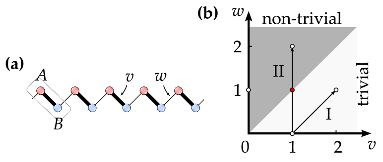
Figure 1: (a) A schematic representation of the 1D SSH model for spinless fermions. $A$ and $B$ denote two sublattices within a unit cell. $v$ and $w$ represent the intra-cell and inter-cell hopping amplitudes, respectively. (b) The phase diagram at half-filling. Two evolutionary paths are indicated by lines with arrows. Path I corresponds to a case where both the initial and final states belong to the trivial phase, while Path II represents a transition to a topologically nontrivial phase. The red dot marks the critical point studied in Ref. [43].

To simulate a fermionic Hamiltonian on a quantum circuit, the first step is to map it onto a qubit basis. Several transformations can be employed for this purpose, including the Jordan-Wigner transformation [48], the Bravyi-Kitave transformation [49], the Ball-Verstracete-Cirac transformation [50, 51], and other recently developed methods [52, 53, 54, 55, 56]. In this work, we adopt the Jordan-Wigner transformation (JWT) [43, 48], which maps fermionic opertors to qubit operators as follows:

$$\hat{c}_{i}^{\dagger} =\sigma_{i}^{-}\hat{K},~~~\hat{c}_{i}=\hat{K}\sigma_{i}^{+},$$ (2)

where $\sigma^{\pm}_{i}=\frac{1}{2}(\hat{X}_{i}\pm i\hat{Y}_{i})$ and $\hat{K}=\exp[-i\frac{\pi}{2}\sum_{j<i}(\hat{Z}_{j}+1)]$ is a nonlocal string operator. Here, $\hat{X}_{i},\hat{Y}_{i},\hat{Z}_{i}$ denotes the Pauli matrices acting on site $i$, with the sublattice index omitted for simplicity.

For the 1D SSH model, which contains only nearest-neighbor hopping terms, the JWT yields the following mapping:

$$\hat{c}^{{\dagger}}_{i}\hat{c}_{i+1}+\text{H.c.}\mapsto\sigma_{i}^{+}\sigma_{i+1}^{-}+\text{H.c.}$$ (3)

for hopping terms that do not cross the boundary. For convenience, let us introduce two sets of natural numbers, $4\mathbb{N}=\{4n\ |n\in\mathbb{N}\}$ and $4\mathbb{N}+2=\{4n+2\ |n\in\mathbb{N}\}$, where $\mathbb{N}$ is the set of natural numbers. For the hopping term across the boundary, the string operator in the JWT becomes trivial when the system size satisfies $L\in 4\mathbb{N}$ for APBCs or $L\in 4\mathbb{N}+2$ for PBCs. This corresponds to a closed-shell condition, where a gap always persists at half filling, except at the critical point $v=w$. Thus, the SSH model can be exactly mapped onto the following qubit model:

$$\hat{\mathcal{H}}_{\text{SSH}}=-\sum_{i=1}^{L/2}\left(v\sigma_{A,i}^{+}\sigma_{B,i}^{-}+w\sigma_{B,i}^{+}\sigma_{A,i+1}^{-}\right)+\text{H.c.}$$ (4)

The total Hamiltonian can be decomposed into two groups, each containing mutually commutable local Hamiltonian terms, i.e.,

$$\hat{\mathcal{H}}_{\text{SSH}}=\hat{\mathcal{H}}_{1}+\hat{\mathcal{H}}_{2},$$ (5)

where

$$\hat{\mathcal{H}}_{1}=-\sum_{i=1}^{L/2}v\sigma_{A,i}^{+}\sigma_{B,i}^{-}+\text{H.c.}$$ (6)

and

$$\hat{\mathcal{H}}_{2}=-\sum_{i=1}^{L/2}\gamma w\sigma_{B,i}^{+}\sigma_{A,i+1}^{-}+\text{H.c.}.$$ (7)

Each term in $\hat{\mathcal{H}}_{i}~(i=1,2)$ involves interactions between only two neighboring qubits. The ground state of an individual term $-(\sigma_{i}^{+}\sigma_{i+1}^{-}+\text{H.c.})$ is simply given by $|{\rm t}\rangle=\frac{1}{\sqrt{2}}\left(|01\rangle+|10\rangle\right)$, which can be easily prepared from the product state $|00\rangle$ using the circuit shown in Fig. 2(a). Therefore, the ground state of $\mathcal{H}_{i}~(i=1,2)$ can be prepared by applying $L/2$ identical copies of this set of gates to neighboring qubits. We choose $\hat{\mathcal{H}}_{i}~(i=1,2)$ as our initial Hamiltonian.

Throughout this paper, we examine the unitary evolution from the ground state of $\hat{\cal{H}}_{1}$ to that of $\hat{\cal{H}}_{\text{SSH}}$ using the DQAP ansatz [43]:

$$|\Psi_{M}({\bm{\theta}})\rangle = \prod_{m=M}^{1}\hat{\mathcal{U}}^{(1)}({\theta_{m}^{(1)},\theta_{m}^{(2)}})|\Psi^{(1)}\rangle$$ (8)

$$= \hat{\mathcal{U}}^{(1)}({\theta_{M}^{(1)},\theta_{M}^{(2)}})\cdots\hat{\mathcal{U}}^{(1)}({\theta_{2}^{(1)},\theta_{1}^{(2)}})\hat{\mathcal{U}}^{(1)}({\theta_{1}^{(1)},\theta_{1}^{(2)}})|\Psi^{(1)}\rangle,$$

where

$$\hat{\mathcal{U}}^{(1)}({\theta_{m}^{(1)},\theta_{m}^{(2)}})=e^{-i\theta_{m}^{(1)}\hat{\mathcal{H}}_{1}}e^{-i\theta_{m}^{(2)}\hat{\mathcal{H}}_{2}}$$ (9)

and $M$ represents the number of time steps with $|\Psi^{(1)}\rangle=|{\rm b}\rangle_{1}\otimes|{\rm b}\rangle_{2}\otimes\cdots\otimes|{\rm b}\rangle_{L/2}$ being the ground state of $\hat{\mathcal{H}}_{1}$. The variational parameters $\{\theta_{m}^{(1)},\theta_{m}^{(2)}\}_{m=1}^{M}$ are optimized by minimizing the expectation value of the energy:

$$E_{M}({\bm{\theta}})=\langle\Psi_{M}({\bm{\theta}})|\hat{\cal H}_{\text{SSH}}|\Psi_{M}({\bm{\theta}})\rangle.$$ (10)

We employ the natural gradient descent method for optimization, where both the gradient and the metric tensor are efficiently calculated as described in Ref. [43]. Since $\hat{\mathcal{H}}_{i}~(i=1,2)$ consists of mutually commutative terms, the time evolution of $\hat{\mathcal{H}}_{i}~(i=1,2)$ can be efficiently parallelized. The time-evolution of the local term $\exp[-i\theta(\sigma_{i}^{+}\sigma_{i+1}^{-}+\text{H.c.})]$ can be exactly implemented using the circuit shown in Fig. 2(b).

Finally, we note that the DQAP ansatz in Eqs. (8-10) at an intermediate step generally does not represent the ground state of the instantaneous Hamiltonian [43] somewhere on the straight line of a Path connecting the start and end points in Fig. 1 (b). Therefore, the straight lines connecting the start and end points in Fig. 1 (b) should be understood as schematics.

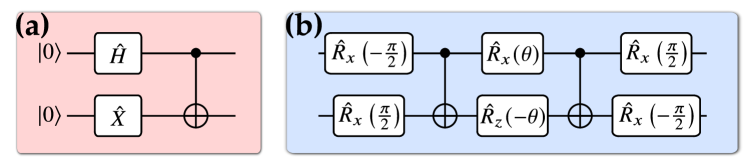
Figure 2: Quantum circuit implementations for (a) the initial state $|\mathrm{t}\rangle=\frac{1}{\sqrt{2}}(|01\rangle+|10\rangle)$ and (b) the unitary time evolution operator $\exp[-i\frac{\theta}{2}(\hat{X}_{i}\hat{X}_{j}+\hat{Y}_{i}\hat{Y}_{j})]$. In the circuits, $\hat{X}$, $\hat{H}$ denote the Pauli-$X$ and Hadamard gates, respectively, while the rotation gates are defined as $\hat{R}_{x}(\theta)=\exp(-i\frac{\theta}{2}\hat{X})$ and $\hat{R}_{z}(\theta)=\exp(-i\frac{\theta}{2}\hat{Z})$. The Cnot gates are represented in the standard form.

III Numerical Results

In this section, we present numerical results obtained using classical computers. The initial state is always set to the ground state of $\hat{\mathcal{H}}_{1}$ with $v=1$, which is equivalent to the ground state of $\hat{\mathcal{H}}_{\rm SSH}$ with $(v,w)=(1,0)$. We then vary the parameters $(v,w)$ in the final Hamiltonian $\hat{\mathcal{H}}_{\rm SSH}$, whose ground state is the target final state in the time evolution [see Fig. 1(b)]. By appropriately tuning $(v,w)$ in the final Hamiltonian, we systematically investigate the two distinct cases: one where the time evolved state remains within the same topologically trivial phase, and another where it transforms into a topologically nontrivial phase. The main results are summarized in Table 1.

III.1 Ground-state energy

Figure 3 shows the energy difference, $\Delta E=E_{L}^{M}({\bm{\theta}}_{\text{opt}})-E_{\text{exact}}(L)$, between the optimized variational ground-state energy $E_{L}^{M}({\bm{\theta}}_{\text{opt}})$ and the exact ground-state energy $E_{\text{exact}}(L)$ for a system size of $L=200$. Here, $E_{L}^{M}({\bm{\theta}}_{\text{opt}})$ is computed using the DQAP ansatz $|\Psi_{M}({\bm{\theta}})\rangle$ with the optimized variational parameters ${\bm{\theta}}=\{\theta_{m}^{(1)},\theta_{m}^{(2)}\}_{m=1}^{M}$, which defines a quantum circuit with a depth of $M$. The optimized variational parameters ${\bm{\theta}}_{\text{opt}}$ for different values of $M$ are provided in Appendix A.3 (see also Figs. 13 and 14). In Fig. 3(a), $w$ is fixed at $1$, while $v$ is varied form $1$ to 4 in the final Hamiltonian. In contrast, in Fig. 3(b), $v$ is fixed at $1$ and $w$ is varied from $1$ to $2$. These choices correspond to different time evolution scenarios: Fig. 3(a) represents an evolution where the system remains in the trivial phase (Path I), while Fig. 3(b) corresponds to a transition from the trivial to the topological phase (Path II). It is important to note that at the critical point $v=w=1$ in the final Hamiltonian, the exact ground state can be prepared when $M=L/4$ for APBCs, as shown in Fig. 3, or $M=(L-2)/4$ for PBCs [43]. This result is consistent with the bound imposed by the information propagation speed in a quantum circuit composed of local quantum gates [57]. The system size dependence of the energy is discussed in Appendix A.1.

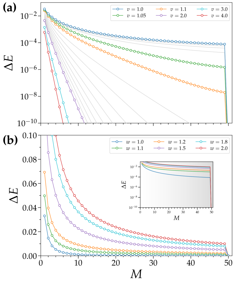
Figure 3: The energy difference $\Delta E$ as a function of circuit depth $M$ for various parameters $(v,w)$ in the final Hamiltonian. The system size is $L=200$ under APBCs. (a) $w$ is fixed at $1$, while $v$ is varied, representing the case where both the initial and final states belong to the trivial phase (case I). (b) $v$ is fixed at $1$, while $w$ is varied, illustrating the case where the initial and final states belong to different topological phases (case II). In (a), thin lines between the results for $v=1.0$ and $v=1.05$ indicate intermediate values from $v=1.01$ to $v=1.04$, while thin lines between $v=1.1$ and $v=2$ correspond to $v=1.2$ to $v=1.9$. The inset of (b) displays a semi-logarithmic plot.

In addition, we observe three notable features in Fig. 3. First, as shown in Fig 3(a), within the parameter range $v\in[1.0,1.1]$ in the final Hamiltonian, the number of layers required to prepare the ground state with extremely high accuracy ($<10^{-8}$) remains a quarter of the system size. This is reasonable since this parameter range is very close to the critical point. Second, as $v$ increases further, $\Delta E$ exhibits a clear exponential decay with respect to $M$. This implies that a shallow circuit, containing fewer quantum gates than in the critical case ($v=1$), is sufficient to prepare the ground state with high accuracy. This observation holds when the initial and final states belong to the same phase and when a large spectrum gap persists. A similar conclusion is expected for cases where both the initial and final states reside in the non-trivial phase, as these cases can be mapped onto each other by a single-site translation. Third, as shown in Fig. 3(b), when the initial and final states belong to different topological phases, the minimal number of layers required to exactly prepare the target ground state is consistently $M=L/4$.

III.2 Entanglement entropy

In Fig. 4, we calculate the evolution of the entanglement entropy, $S_{\mathbb{A}}=-\text{Tr}\rho_{\mathbb{A}}\ln\rho_{\mathbb{A}}$, for two different cases. Here, $\rho_{\mathbb{A}}=\text{Tr}_{\overline{\mathbb{A}}}|\Psi_{M}({\bm{\theta}}_{\rm opt})\rangle\langle\Psi_{M}({\bm{\theta}}_{\rm opt})|$ is the reduced density matrix of the optimized state $|\Psi_{M}({\bm{\theta}}_{\rm opt})\rangle$ for subsystem $\mathbb{A}$. We consider a half-system bipartition into contiguous subsystems $\mathbb{A}$ and its complement $\overline{\mathbb{A}}$, placing the entanglement cuts on $w$-bonds (i.e., bonds between unit cells). Details of the calculation can be found in Ref. [43]. In Fig. 4(a), where both the initial and final states belong to the trivial phase (Path I), we observe that $S_{\mathbb{A}}$ saturates at approximately $0.355$ after only four layers. This indicates that in the gapped case, the two halves of the system are weakly entangled, and a shallow circuit of depth $M=4$ is sufficient to generate the necessary quantum entanglement between subsystems $\mathbb{A}$ and $\overline{\mathbb{A}}$ in the target state.

Figure 4: Entanglement entropy $S_{\mathbb{A}}$ as a function of circuit depth $M$ for various system sizes $L$ under APBCs. (a) and (b) show the results for the parameters $(v,w)=(2.0,1.0)$ and $(1.0,1.1)$ in the final Hamiltonian, respectively, corresponding to Path I and Path II in Fig. 1(a). The variational parameters $\bm{\theta}$ in the DQAP ansatz $|\Psi_{M}(\bm{\theta})\rangle$ are optimized for each $L$ and $M$. For comparison, the results for the case where $L$ and $M$ are varied while maintaining $L=8M$ are also shown by a read line. Additionally, the entanglement entropy for the exact ground state of the final Hamiltonian with the system size $L$ is plotted at $L=4M$ using a magenta line.

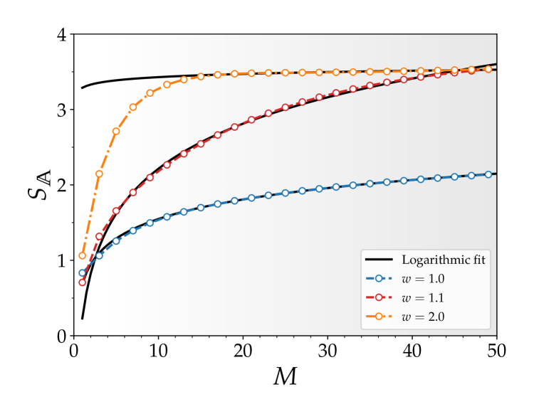
Figure 5: Logarithmic fitting (solid lines) of the entanglement entropy $S_{\mathbb{A}}$ for $M=L/8$ (circles), obtained using the optimzed DQAP ansatze $|\Psi_{M}(\bm{\theta})\rangle$ for various system sizes $L$. The fitting parameters $(a,b)$ for the form $\tilde{S}_{\mathbb{A}}=a\ln{M}+b$ are $(0.3709,0.6942)$, $(0.8619,0.2300)$, and $(0.0612,3.2880)$ for the parameter sets $(v,w)=(1.0,1.0)$, $(1.0,1.1)$ and $(1.0,2.0)$, respectively.

In Fig. 4(b), where the initial and final states belong to different topological phases (Path II), the entanglement entropy $S_{\mathbb{A}}$ exhibits a clearly nonmonotonic dependence on the number $M$ of circuit layers. We note that such nonmonotonic behavior was not observed clearly in the previous study at the critical point $v=w=1$ [43]. Upon closer examination of its dependence on $M$, we find that $S_{\mathbb{A}}$ initially increases, following a universal, system-size independent curve for $M<L/8$. This behavior can be understood in terms of operator spreading: two-qubit gates acting on the two boundaries between $\mathbb{A}$ and $\overline{\mathbb{A}}$ do not overlap in the DQAP ansatz as long as $M<L/8$ [43]. Specifically, the entanglement between $\mathbb{A}$ and $\overline{\mathbb{A}}$ is first generated by two-qubit gates on the boundaries at $M=1$, and for $M<L/8$, the supports of these operators remain non-overlapping, leading to a system-size independent $S_{\mathbb{A}}$.

To gain insights into the universal behavior of the entanglement entropy $S_{\mathbb{A}}$ for $M=L/8$, we fit the data obtained for various system sizes $L$ using the following form [58]:

$$\tilde{S}_{\mathbb{A}}=a\ln{M}+b,$$ (11)

where $a$ and $b$ are fitting parameters. Figure 5 shows the fitting results for the parameter sets $(v,w)=(1.0,1.0),(1.0,1.1)$, and $(1.0,2.0)$. We find that the entanglement entropy $S_{\mathbb{A}}$ fits well to a logarithm form for larger $M$, even when the target ground state is not at criticality.

At $M=L/8$, $S_{\mathbb{A}}$ begins to deviate from the universal curve and, almost simultaneously, starts decreasing as $M$ increases. $S_{\mathbb{A}}$ finally reaches the exact value of the final Hamiltonian $\hat{\cal H}_{\rm SSH}$ at $M=L/4$, exhibiting a discontinuity. Notably, the system-size dependence of the exact values is insignificant, as indicated by the magenta line in Fig. 4(b). This implies that the entanglement entropy $S_{\mathbb{A}}$ of the ground state at $(v,w)=(1.0,1.1)$ follows the area-law scaling, in contrast to the critical case, where the entanglement entropy increases logarithmically with the subsystem size [59]. While the convergence of $S_{\mathbb{A}}$ to the exact value at $M=L/4$ is expected, the observed clear discontinuity as a function of circuit depth $M$ was not found in the previous study for the critical case [43]. These finding suggests a nontrivial information spreading process during the unitary evolution from the trivial to the topological phase under the DQAP ansatz.

III.3 Mutual information

To further examine the information spreading process under the DQAP ansatz, we compute the mutual information. The mutual information between two parts of the system is defined as $I_{\mathbb{A},\mathbb{B}}=S_{\mathbb{A}}+S_{\mathbb{B}}-S_{\mathbb{A}\cup\mathbb{B}}$, which quantities the entanglement between the two parts $\mathbb{A}$ and $\mathbb{B}$ of the system. Fixing the system size at $L=200$, we define subsystem $\mathbb{A}$ as two sites at the 99th and 100th sites (i.e., the 50th unit cell, corresponding to a $v$-bond), while subsystem $\mathbb{B}$ consists of a single site, whose location is varied. Figure 6 shows the mutual information for Path I and Path II. For Path I, the mutual information remains spatially localized around the reference subsystem $\mathbb{A}$ throughout the entire evolution process. In contrast, for Path II, the mutual information gradually spreads across the system and extends throughout the whole system by the time the circuit depth reaches $M=L/8$. It then remains spread across the entire system until $M=L/4-1$, just one layer before reaching the exact ground state of the target Hamiltonian $\hat{\cal H}_{\rm SSH}$ with $(v,w)=(1,2)$. Finally, at $M=L/4$, the mutual information abruptly localized around the reference subsystem $\mathbb{A}$. This sudden change of mutual information at the final layer is compatible with the discontinuous behavior of the entanglement entropy observed in Fig. 4(b). A further analysis of the mutual information can be found in Appendix A.2.

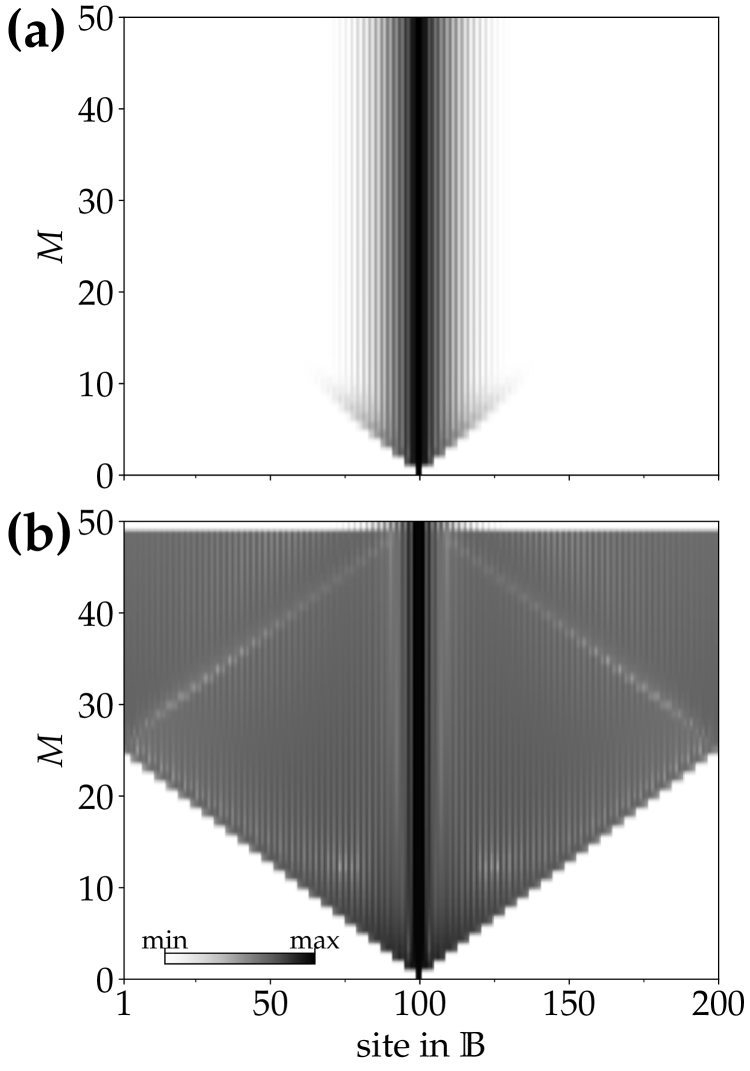
Figure 6: Intensity plot of the mutual information $I_{\mathbb{A},\mathbb{B}}$ for the optimized DQAP ansatz $|\Psi_{M}(\bm{\theta})\rangle$, shown as a function of the circuit depth $M$ and the location of the single site composing subsystem $\mathbb{B}$. (a) and (b) correspond to the cases with the parameters $(v,w)=(2,1)$ and $(1,2)$ in the final Hamiltonian, respectively, representing Path I and Path II in Fig. 1(a). The system size is set to $L=200$ under APBCs and the DQAP ansatz $|\Psi_{M}(\bm{\theta})\rangle$ is optimized for each $M$. Subsystem $\mathbb{A}$ consists of two sites locating at the center of the system. White color in the intensity plots represent zero.

III.4 Polarization

Having observed the nontrivial information-spreading process along Path II under the DQAP ansatz, a natural question arises: At what circuit depth $M$ does the ansatz state $|\Psi_{M}({\bm{\theta}})\rangle$ undergo a topological transition? To address this, we compute the polarization defined as [47, 60]

$${\cal P}_{\rm R}(M)={\rm Im}\ln\langle\Psi_{M}({\bm{\theta}}_{\rm opt})|\hat{\cal U}_{\rm R}|\Psi_{M}({\bm{\theta}}_{\rm opt})\rangle,$$ (12)

where the unitary operator $\hat{\cal U}_{\rm R}$ is defined as

$$\hat{\cal U}_{\rm R} ={\exp}\left[\frac{2\pi i}{(L/2)}\sum_{j=1}^{L/2}\left(\left(j-\frac{1}{2}\right)\hat{c}_{A,j}^{\dagger}\hat{c}_{A,j}+j\hat{c}_{B,j}^{\dagger}\hat{c}_{B,j}\right)\right]$$

$$={\exp}\left[\frac{2\pi i}{L}\sum_{l=1}^{L}l\hat{c}_{l}^{\dagger}\hat{c}_{l}\right]$$

$$=\prod_{l=1}^{L}{\exp}\left[\frac{2\pi i}{L}l\hat{c}_{l}^{\dagger}\hat{c}_{l}\right].$$ (13)

Here, $l$ represents the site index, serving as a one-dimensional label that runs over both unit-cell and sublattice indexes $j$, $A$, and $B$. Specifically, we define $l=2j-1$ ($l=2j$) for sites belonging to sublattice $A$ ($B$) of the $j$th unit cell. The last equality in Eq. (13) holds because fermion density operators commute with each other.

The polarization ${\cal P}_{\rm R}(M)$ depends on the choice of the origin for the “position” $l$ in front of $\hat{c}_{l}^{\dagger}\hat{c}_{l}$ in Eq. (13). However, the difference

$$\Delta{\cal P}_{\rm R}(M)={\cal P}_{\rm R}(M)-{\cal P}_{\rm R}(0)$$ (14)

allows for an unambiguous detection of the topological phase transition during the DQAP evolution. Figure 7 shows the calculated polarization as a function of the circuit depth $M$ for various system sizes $L\in 4\mathbb{N}$ along Path II. As expected, the polarization takes different values in the initial $(M=0)$ and final $(M=L/4)$ states, indicating the occurrence of a topological phase transition during the DQAP evolution.

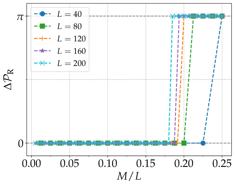
Figure 7: The polarization difference $\Delta{\cal P}_{\rm R}(M)$ as a function of the circuit depth $M$ for various system sizes $L$. The variational parameters $\bm{\theta}$ in the DQAP ansatz $|\Psi_{M}(\bm{\theta})\rangle$ are optimized for each $M$ and $L$. The parameters in the final Hamiltonian are set to $(v,w)=(1.0,1.1)$, corresponding to Path II in Fig. 1(b).

Interestingly, the critical circuit depth $M^{*}$ at which ${\cal P}_{R}(M)$ changes,

$${\cal P}_{\rm R}(M^{*})-{\cal P}_{\rm R}(M^{*}-1)\neq 0,$$ (15)

does not generally coincide with the final step. This suggests that the topological phase transition occurs during the DQAP evolution, before reaching the exact ground state of the final Hamiltonian. Figure 8 shows $M^{*}$ as a function of the the system size $L$ for two different parameter sets, $(v,w)=(1,1.1)$ and $(1,2)$, in the final Hamiltonian. We observe that $M^{*}$ exhibits a staircase-like increase with $L$. Although it is not conclusive, our numerical results suggest that the critical $M^{*}$ satisfies $L/8\leqslant M^{*}\leqslant L/4$ for $L\in 4\mathbb{N}$ and $(L-2)/8\leqslant M^{*}\leqslant(L-2)/4$ for $L\in 4\mathbb{N}+2$, where the lower bound corresponds to the circuit depth at which the causal cone spans the entire system [see Fig. 6(b) and Ref. [43]]. Remarkably, if the topological phase transition occurs before the final step, no discontinuities in ground-state energy, entanglement entropy, or mutual information are observed at $M=M^{*}$.

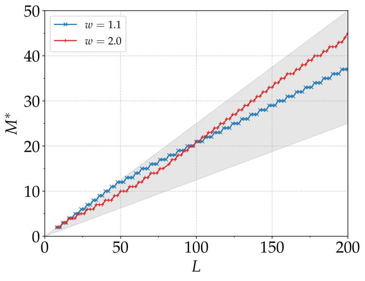
Figure 8: The critical circuit depth $M^{*}$ as a function of the system size $L$. The parameters of the final Hamiltonian are set to $(v,w)=(1.0,1.1)$ and $(1.0,2.0)$. APBCs are imposed for $L\in 4\mathbb{N}$, while PBCs are used for $L\in 4\mathbb{N}+2$. The shaded region indicates $L/8\leqslant M^{*}\leqslant L/4$.

IV Experiments on quantum hardware

Exploring topological phase transitions poses a significant challenge for near-term noisy quantum devices, as topological order parameters are inherently nonlocal, as seen in Eq. (13). Nevertheless, a seminal study [19] successfully demonstrated a topological phase transition in a spin chain by evaluating topological order parameters using IBM’s superconducting quantum computers. Here, in this work, we employ Quantinuum’s trapped-ion quantum computer to evaluate the polarization ${\cal P}_{\rm R}$ as a topological order parameter. We further detail how the abrupt change in polarization can be detected with a real quantum device.

The experiments were conducted in January 2024 using the H1-1 system by Quantinuum [46]. At the time of the experiments, the H1-1 system consisted of $20$ qubits and natively supported single-qubit rotation gates and two-qubit ZZ phase gates defined as ${\rm ZZPhase}(\alpha)=e^{-\frac{1}{2}i\pi\alpha\hat{Z}_{i}\hat{Z}_{j}}$, parametrized by a real angle $\alpha$. These native two-qubit native gates could be applied between an arbitrary pair of qubits. The average infidelity of single-qubit and two-qubit gates was about $0.004\%$ and $0.2\%$, respectively, while state preparation and measurement errors averaged $0.3\%$. Further details on the hardware specifications can be found in Ref. [46]. All quantum circuits used in the experiments were compiled using TKET [61].

Table 2: The optimized variational parameters $\bm{\theta}_{\rm opt}=\{\theta_{m}^{(1)},\theta_{m}^{(2)}\}_{m=1}^{M}$ obtained from classical simulations for $L=18$ under PBCs, which are subsequently used for the experiments.

	$M=1$	$M=2$	$M=3$	$M=4$
$\theta_{1}^{(1)}$	0.7853981636	1.2494387001	1.3583873392	1.4379338692
$\theta_{1}^{(2)}$	0.2767871793	0.2688075377	0.2534789267	0.5229341500
$\theta_{2}^{(1)}$	–	0.6392420907	1.1586546608	1.4498686393
$\theta_{2}^{(2)}$	–	0.4831535535	0.5146221144	0.7033476173
$\theta_{3}^{(1)}$	–	–	0.5714210664	1.4215754149
$\theta_{3}^{(2)}$	–	–	0.5376954104	0.7169480772
$\theta_{4}^{(1)}$	–	–	–	1.0837464017
$\theta_{4}^{(2)}$	–	–	–	0.6676928002

We consider the 1D SSH model of $L=18$ sites under PBCs, setting the parameters $(v,w)=(1,2)$ in the final target Hamiltonian. Every single site is mapped to a single qubit via the JWT, as described in Sec. II. Additionally, we introduce an ancillary qubit for the Hadamard test, bringing the total number of qubits used to $L+1=19$. The number of circuit layers is varied within the range $0\leqslant M\leqslant 4=(L-2)/4$. To optimize quantum resource utilization, the optimal variational parameters $\bm{\theta}_{\rm opt}$ are pre-determined through classical simulations (see Table 2), allowing us to bypass the iterative parameter optimization process between quantum and classical computers.

The polarization given in Eq. (12) can be reformulated for quantum computation as

$${\cal P}_{\rm R}(M)=\arctan{\left(\frac{y}{x}\right)}$$ (16)

with

$$x ={\rm Re}\langle\Psi_{M}(\bm{\theta}_{\rm opt})|\hat{\cal U}_{\rm R}|\Psi_{M}(\bm{\theta}_{\rm opt})\rangle,$$ (17)

$$y ={\rm Im}\langle\Psi_{M}(\bm{\theta}_{\rm opt})|\hat{\cal U}_{\rm R}|\Psi_{M}(\bm{\theta}_{\rm opt})\rangle.$$ (18)

We evaluate $x$ and $y$ separately on a quantum computer using the Hadamard test. The uncertainty in the polarization, arising from the measurement of these quantities, is estimated using the error propagation formula: $\delta{\cal P}_{\rm R}=\sqrt{\left(\frac{\partial{\cal P}_{\rm R}}{\partial x}\delta x\right)^{2}+\left(\frac{\partial{\cal P}_{\rm R}}{\partial y}\delta y\right)^{2}}=\sqrt{\left(\frac{xy}{x^{2}+y^{2}}\right)^{2}\left(\frac{\delta x^{2}}{x^{2}}+\frac{\delta y^{2}}{y^{2}}\right)},$ where $\delta x$ and $\delta y$ are the standard errors in the measurement of $x$ and $y$, respectively.

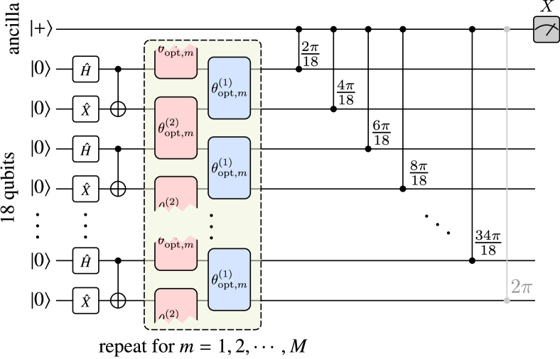
Figure 9: The quantum circuit to evaluate the real part $x={\rm Re}\langle\Psi_{M}(\bm{\theta}_{\rm opt})|\hat{\cal U}_{\rm R}|\Psi_{M}(\bm{\theta}_{\rm opt})\rangle$ for $L=18$ under PBCs. The topmost qubit represents the ancillary qubit used for the Hadamard test, while the remaining 18 qubits correspond to the system qubits, on which the DQAP state $|\Psi_{M}({\bm{\theta}}_{\rm opt})\rangle$ is prepared. The leftmost part of the circuit, consisting of qubit initialization, Hadamard gates, Pauli $X$ gates, and CNOT gates, construct the initial state $|\Psi^{(1)}\rangle$, which represents the ground state of $\hat{\cal H}_{1}$. The section inside the dashed box represents the DQAP ansatz unitary, $\prod_{m=M}^{1}\hat{\cal U}^{(1)}(\theta_{m}^{(1)},\theta_{m}^{(2)})$, with the optimized variational parameters determined from classical simulations (see Table. 2). Blue and red rounded rectangles denote the two-qubit gates $\exp[-i\frac{\theta_{m}^{(1)}v}{2}(\hat{X}_{i}\hat{X}_{j}+\hat{Y}_{i}\hat{Y}_{j})]$ and $\exp[-i\frac{\theta_{m}^{(2)}w}{2}(\hat{X}_{i}\hat{X}_{j}+\hat{Y}_{i}\hat{Y}_{j})]$, respectively. The sequence of controlled-phase gates corresponds to the ${\rm C}_{0}{\text{-}}\hat{\cal U}_{\rm R}$ operation in Eq. (19). Notice that the controlled-phase gate ${\rm C}_{0}{\text{-}}{\rm Phase}_{l}(2\pi l/L)$ for $l=L$ (light gray) is the identity operation and is therefore omitted from the circuit.

Figure 9 illustrates the quantum circuit to evaluate the real part $x$. First, the state $|\Psi_{M}(\bm{\theta}_{\rm opt})\rangle$ is prepared by applying $M$ layers of the DQAP ansatz unitary $\prod_{m=M}^{1}\hat{\cal U}^{(1)}(\theta_{m}^{(1)},\theta_{m}^{(2)})$ to the initial state $|\Psi^{(1)}\rangle$, which is a product of $|{\rm t}\rangle$ and corresponds to the ground state of $\hat{\cal H}_{1}$. Second, the controlled-$\hat{\cal U}_{\rm R}$ operation is implemented as follows:

$${\rm C}_{0}{\text{-}}\hat{\cal U}_{\rm R}=\prod_{l=1}^{L}{\rm C}_{0}{\text{-}}{\rm Phase}_{l}\left(\frac{2\pi l}{L}\right),$$ (19)

where ${\rm C}_{0}{\text{-}}\hat{\cal U}_{\rm R}$ represents the unitary operation of $\hat{\cal U}_{\rm R}$ on the system qubits ($1$st to $L$th registers) controlled by an ancillary qubit ($0$th register). The controlled-phase gate ${\rm C}_{0}{\text{-}}{\rm Phase}_{l}(\theta)={\rm diag}(1,1,1,{\rm e}^{i\theta})$ acts with a control on the $0$th qubit and a target on the $l$th qubit. Since ${\rm C}_{0}{\text{-}}{\rm Phase}_{l}\left(\frac{2\pi l}{L}\right)$ for $l=L$ is the identity operation, the implementation of ${\rm C}_{0}{\text{-}}\hat{\cal U}_{\rm R}$ requires $L-1$ controlled-phase gates. Finally, the real part $x$ is obtained by measuring the expectation value of the Pauli $X$ operator on the ancillary qubit. Similarly, the imaginary part $y$ is determined using the same quantum circuit, except that the ancillary qubit is measured in the Pauli $Y$ basis instead of $X$. Notice that these quantum circuits are further compiled for the H1-1 system for execution. The number of native two-qubit gates required on the H1-1 system for various circuit depth $M$ are 26, 62, 98, 134, and 170 for $M=$ 0, 1, 2, 3, and 4, respectively (see Appendix B).

Figure 10(a) shows the experimentally evaluated results for $x$ and $y$, as defined in Eqs. (17) and (18), for $M=0,1,2,3,$ and $4$ using the H1-1 system. Each value of $x$ and $y$ was estimated with 500 measurements for $M=0,1,2,4$ and 2000 measurements for $M=3$ to ensure a sufficiently small uncertainty $\delta{\cal P}_{\rm R}$. The larger number of measurements for $M=3$ was necessary because both $x$ and $y$ are closer to zero, leading to a larger uncertainty in the polarization, which is nothing but the argument of the complex number $x+iy$. If the number of measurements were set to a similar value, this would results in an increased statistical uncertainty [see also the expression for $\delta{\cal P}_{\rm R}$ immediately after Eq. (18)]. In general, a greater number of measurements is required in the vicinity of the topological phase transition to maintain a given level of precision. Conversely, if the number of measurements remains fixed, an increase in the uncertainty $\delta{\cal P}_{\rm R}(M)$ can serve as an indicator of the topological phase transition, i.e., at $M\sim M^{*}$. For comparison, we also include noiseless simulation results obtained from the H1-1E emulator provided by Quantinuum, using the same number of measurements. The experimental results show qualitative agreement with these noiseless simulations. For $M\leqslant 3$, the results lie along the negative side of the $y$-axis, implying that ${\cal P}_{\rm R}(M)=\arctan\left(\frac{y}{x}\right)\approx-\frac{\pi}{2}$. For $M=4$, the results shift to the positive side of the $y$-axis, indicating that ${\cal P}_{\rm R}(M)=\arctan\left(\frac{y}{x}\right)\approx\frac{\pi}{2}$.

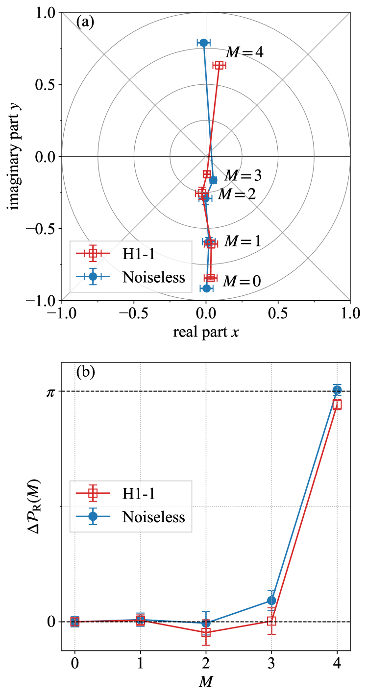
Figure 10: (a) Real and imaginary parts of $\langle\Psi_{M}(\bm{\theta}_{\rm opt})|\hat{\cal U}_{\rm R}|\Psi_{M}(\bm{\theta}_{\rm opt})\rangle$ for $M=0$ to 4 (from bottom to top). Circular and straight lines are guide to the eyes. (b) Polarization difference $\Delta{\cal P}_{\rm R}(M)$ as a function of circuit depth $M$. Red squares represent the experimental results obtained using the H1-1 system, while blue circles denote the noiseless simulation results. Dashed horizontal lines are guide to the eyes. The parameters of the final target Hamiltonian are set to $(v,w)=(1,2)$, corresponding to Path II in Fig. 1(b).

Figure 10(b) shows the polarization difference $\Delta{\cal P}_{\rm R}(M)$, evaluated using the values of $x$ and $y$ shown in Fig. 10. Despite being obtained without any error mitigation, the experimental results show good quantitative agreement with the noiseless simulations. Specifically, the polarization at $M=4$ is clearly distinct from those at $M\leqslant 3$. The robustness of these results against noise can be attributed to the behavior observed in Fig. 10: a small perturbation in $x$ and $y$ does not affect the sign of $\arctan\left(\frac{y}{x}\right)$. In particular, the substantial change in the polarization ${\cal P}_{\rm R}(M)$ primarily arises the sign change in $y$ (see also additional experimental results in Appendix C). These findings confirm that our optimized variational state $|\Psi_{M}({\bm{\theta}}_{\rm opt})\rangle$ successfully captures the transition between topologically distinct ground states of the SSH model as the circuit depth $M$ increases, even in the presence of noise in a real quantum device.

V Conclusions

We have applied the DQAP ansatz to obtain the ground state of the 1D SSH model of spinless fermions at half filling, considering various topological phases to which the initial and final states belong. We have found that, irrespective of the topological nature of the initial and final states, the circuit depth $M$ required to exactly prepare the target final ground state is $L/4$ for $L\in 4\mathbb{N}$ under APBCs and $(L-2)/4$ for $L\in 4\mathbb{N}+2$ under PBCs. This is the same circuit depth necessary to obtain the exact ground state at the critical point when starting from a topologically trivial phase [43]. On the other hand, we have also identified qualitatively distinct behaviors in the ground-state energy, entanglement entropy, and mutual information during the DQAP evolution, depending on the topological nature of the initial and final states, as summarized in Table 1. One important finding is that as long as the initial and final states belong to the same phase, only a few layers are sufficient to obtain the target ground state with high accuracy. Additionally, we have numerically computed the polarization as an indicator to distinguish topologically different phases during the DQAP evolution.

We have also demonstrated that the topological phase transition during the DQAP evolution for the 18-site system can be detected by using a trapped-ion quantum computer. The all-to-all connectivity of the trapped-ion quantum computer provided by Quantinuum enables direct evaluation of the polarization, which is derived from the expectation value of a global unitary operator $\hat{{\cal U}}_{\rm R}$, without introducing additional SWAP operations. This capability allows us to effectively characterize the phases experimentally to which the DQAP state belongs. The present results lay the foundation for the next crucial step–exploring topological phases in interacting systems [62, 63] using quantum computers–which we leave for future work.

VI Achnowledgement

A part of this work is based on results obtained from project JPNP20017, subsidized by the New Energy and Industrial Technology Development Organization (NEDO). This study is also supported by JSPS KAKENHI Grants No. JP21H04446, No. JP22K03479, and No. JP22K03520. We further acknowledge funding from JST COI-NEXT (Grant No. JPMJPF2221) and the Program for Promoting Research of the Supercomputer Fugaku (Grant No. MXP1020230411) from MEXT, Japan. Additionally, we appreciate the support provided by the UTokyo Quantum Initiative, the RIKEN TRIP initiative (RIKEN Quantum), and the COE research grant in computational science from Hyogo Prefecture and Kobe City through the Foundation for Computational Science. The numerical simulations have been performed using the HOKUSAI BigWaterfall system at RIKEN (Project IDs: Q23604).

Appendix A Additional numerical results

In this Appendix, we present additional numerical results for the DQAP ansatz applied to the 1D SSH model.

A.1 Energy per site

For the 1D SSH model of spinless fermions at half filling, the ground-state energy per site $\varepsilon_{\infty}$ in the thermodynamic limit is given by

$$\varepsilon_{\infty}=\frac{(v+w)}{\pi}\mathcal{E}_{2}\left(\frac{\pi}{2},\frac{4vw}{(v+w)^{2}}\right),$$ (20)

where

$$\mathcal{E}_{2}(\phi,m)=\int_{0}^{\phi}\sqrt{1-m\sin^{2}\theta}d\theta$$ (21)

denotes the incomplete elliptic integral of the second kind. Figure 11 shows the energy difference per site, $\Delta\varepsilon=E_{L}^{M}(\bm{\theta}_{\rm opt})/L-\varepsilon_{\infty}$, between the variational ground state and the exact ground state in the thermodynamic limit. Here, $E_{L}^{M}(\bm{\theta}_{\rm opt})$ is the variational energy obtained using the DQAP ansatz with the optimized variational parameters $\bm{\theta}_{\rm opt}=\{\theta_{m}^{(1)},\theta_{m}^{(2)}\}_{m=1}^{M}$, consisting of $M$ layers, for a system size $L$. We find that when $M<L/4$, $\Delta\varepsilon$ remains independent of the system size $L$. This behavior arises because quantum entanglement in a quantum circuit composed of local two-qubit gates propagates within a causality-cone-like structure during time evolution. As a result, the quantum gates that contribute to the energy expectation value are confined within this causality cone, making $\Delta\varepsilon$ unaffected by the system size. A detailed analysis of this effect can be found in Refs. [43] and [64].

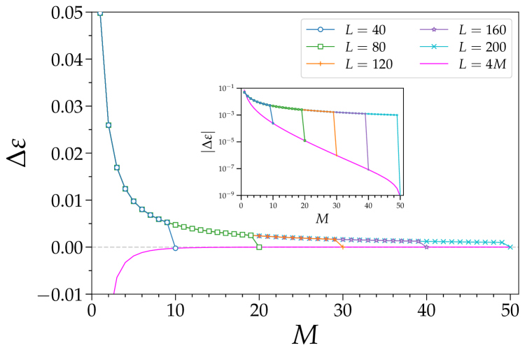
Figure 11: The energy difference per site, $\Delta\varepsilon=E_{L}^{M}(\bm{\theta}_{\rm opt})/L-\varepsilon_{\infty}$, for various system sizes $L$, where $\varepsilon_{\infty}=\lim_{L\to\infty}E_{\rm exact}(L)/L$ and $E_{\rm exact}(L)$ is the exact ground-state energy for a system size $L$. The parameters in the final Hamiltonian are set to $(v,w)=(1,1.1)$, and $L$ is chosen as $L\in 4\mathbb{N}$ under APBCs. The magenta line represents $\Delta\varepsilon_{A}=E_{\rm exact}(L)/L-\varepsilon_{\infty}$ with $L=4M$. The inset shows a semi-logarithmic plot.

A.2 Mutual information for a DQAP ansatz with a fixed $M$

It is also insightful to examine how the mutual information $I_{\mathbb{A},\mathbb{B}}$ evolves as the number $m\,(\leqslant M)$ of layers increases in the DQAP ansatz $|\Psi_{M}(\bm{\theta})\rangle$, where the variational parameters $\bm{\theta}=\{\theta_{m}^{(1)},\theta_{m}^{(2)}\}_{m=1}^{M}$ are optimized for a given $M$. Figure 12 shows the representative results for the mutual information $I_{\mathbb{A},\mathbb{B}}$ in a system of size $L=200$, where subsystem $\mathbb{A}$ consists of two sites located at the center (i.e., at the 99th and 100th sites), while subsystem $\mathbb{B}$ contains a single site whose position is varied (see Sec. III.3 and Fig. 6). Note that the variational parameters in the DQAP ansatz $|\Psi_{M}(\bm{\theta})\rangle$ are optimized for $M=49$ in Fig. 12(a), which is one layer short of reaching the exact ground state, and for $M=50$ in Fig. 12(b), corresponding to the exact ground state of the final target Hamiltonian with $(v,w)=1,2$, which follows Path II in Fig. 1(b). As shown in Fig. 12, in both cases, the entanglement gradually expands in space as the number $m$ of layers increases, forming a causal cone that defines the maximum propagation speed of information with local two-qubit gates, until it spans the entire system at $m=L/8$. However, beyond this point, the behavior of entanglement evolution differs: for $M=49$, the entanglement remains extended across the whole system, while for $M=50$, as the number $m$ of layers further increases, the entanglement gradually contracts, becoming more localized around the center of the system.

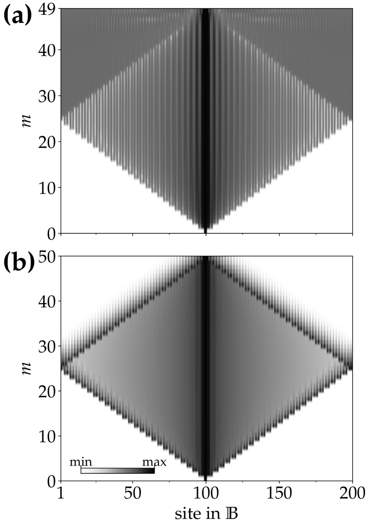
Figure 12: Intensity plot of the mutual information $I_{\mathbb{A},\mathbb{B}}$ for the optimized DQAP ansatz $|\Psi_{M}(\bm{\theta})\rangle$ with (a) $M=49$ and (b) $M=50$, shown as a function of the circuit depth $m$ and the location of the single site composing subsystem $\mathbb{B}$. Here, the system size is set to $L=200$ under APBCs and subsystem $\mathbb{A}$ consists of two sites located at the center of the system, i.e., at the 99th and 100th sites (see Sec. III.3 and Fig. 6). The parameters of the final target Hamiltonian are set to $(v,w)=(1,2)$, corresponding to Path II in Fig. 1(b). For each circuit depth $m$, only the first $m$ values of the optimized variational parameters $\{\theta_{m^{\prime}}^{(1)},\theta_{m^{\prime}}^{(2)}\}_{m^{\prime}=1}^{M}$ are used to compute the mutual information. In contrast, in Fig. 6, the variational parameters are optimized for each $M$. White color in the intensity plots represent zero.

A.3 Optimized variational parameters

Figures 13 and 14 summarize the optimized parameters $\bm{\theta}_{\text{opt}}$ in the DQAP ansatz $|\Psi_{M}(\bm{\theta})$ with $\bm{\theta}=\{\theta_{m}^{(1)},\theta_{m}^{(2)}\}_{m=1}^{M}$ for the target final Hamiltonian with $(v,w)=(1,1.1)$ and $(1.1,1)$, respectively. These correspond to Path II (where the initial and final states belong to different topological phases) and Path I (where both the initial and final states belong to the same topologically trivial phase) in Fig. 1(b). Figures 13(a) and 13(b) [Figures 14(a) and 14(b)] show the optimized parameters for the case of Path II (Path I), where the system size $L\,(\in 4\mathbb{N})$ is varied with $M=L/4$. Therefore, the optimized DQAP ansatz $|\Psi_{M}(\bm{\theta})\rangle$ represents the exact ground state of the target final Hamiltonian. We observe that these optimized parameters vary smoothly as $L$ increases.

Figures 13(c) and 13(d) [Figures 14(c) and 14(d)] show the optimized parameters for the case of Path II (Path I) with $M<L/4$, where the optimized parameters in the DQAP ansatz $|\Psi_{M}(\bm{\theta})\rangle$ for each $M$ are independent of the system size $L$. Specifically, the optimized parameters $\{\theta_{m}^{(1)},\theta_{m}^{(2)}\}_{m=1}^{M}$ for a system size $L_{1}$ are exactly the same as those for a system size $L_{2}$, as long as $4M<L_{1},L_{2}$, assuming that $L_{1},L_{2}\in 4\mathbb{N}$ under APBCs. This behavior arises because the variational parameters $\bm{\theta}$ in the DQAP ansatz $|\Psi_{M}(\bm{\theta})\rangle$ are optimized to minimize the expectation value of energy for the target final Hamiltonian, and the causality cone relevant to this energy expectation value does not extend across the entire system as long as $M<L/4$ [43]. As shown in these figures, we also observe that the optimized parameters vary smoothly with increasing $M$, which are clearly different from those in Figures 13(a) and 13(b) [Figures 14(a) and 14(b)]. Consequently, when the system size $L$ is fixed and $M$ is varied, discontinuous changes appear in the optimized parameters at $M=L/4$ and $M=L/4-1$, as indicated in read and blue in Figs. 13(e) and 13(f) for the case of Path II and in Figs. 14(e) and 14(f) for the case of Path I, although these discontinuities are less pronounced in the latter. This discontinuity is consistent with the abrupt changes observed in the ground-state energy [Fig. 3(b)], entanglement entropy [Fig. 4(b)], and mutual information [Fig. 6(b)].

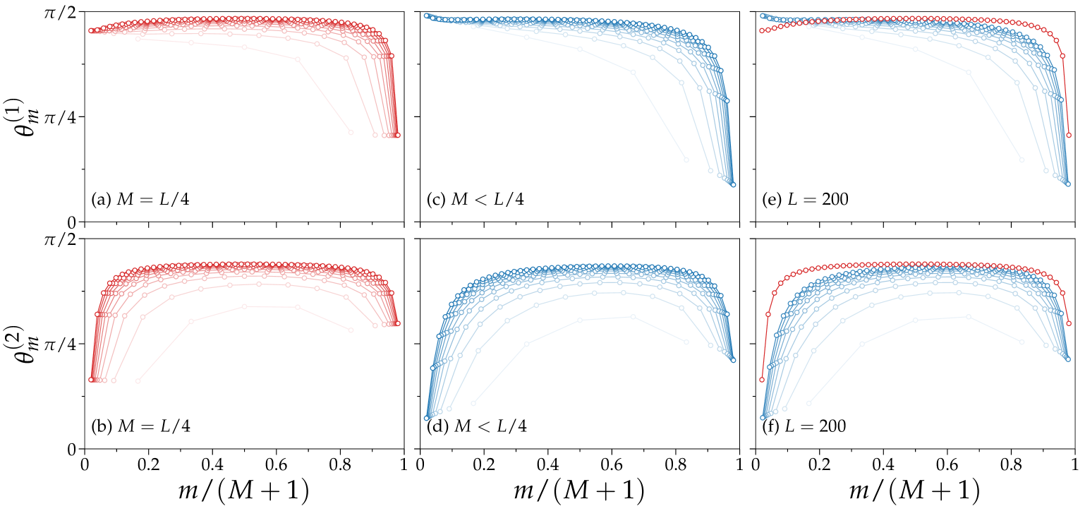
Figure 13: Optimized variational parameters ${\bm{\theta}}_{\text{opt}}$ for $(v,w)=(1.0,1.1)$, corresponding to Path II. (a, b) ${\bm{\theta}}_{\text{opt}}$ for various system sizes up to $L=200$ with $M=L/4$, where the exact ground state state is successfully prepared. (c, d) ${\bm{\theta}}_{\text{opt}}$ for $M<L/4$ with $M$ up to 50. Note that as long as $M<L/4$, the optimized variational parameters are independent of the system size $L$, for which the DQAP ansatz $|\Psi_{M}(\bm{\theta})\rangle$ with $\bm{\theta}=\{\theta_{m}^{(1)},\theta_{m}^{(2)}\}_{m=1}^{M}$ is optimized. (e, f) ${\bm{\theta}}_{\text{opt}}$ for a fixed system size $L=200$, where the DQAP ansatz $|\Psi_{M}(\bm{\theta})\rangle$ is optimized for different $M$. A clear discontinuity in the sets of the optimized parameters is observed between $M=50$ (indicated in red) and $M<50$ (indicated in blue), which is consistent with the abrupt variations in the ground-state energy [Fig. 3(b)], entanglement entropy [Fig. 4(b)], and mutual information [Fig. 6(b)].

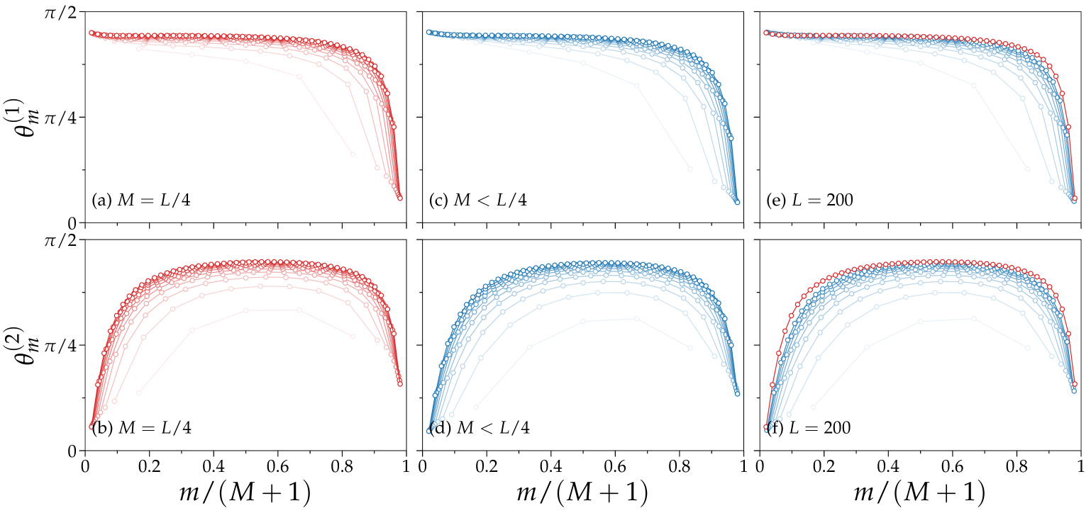
Figure 14: Same as Fig. 13, except that the parameters in the target final Hamiltonian are set to $(v,w)=(1.1,1)$, corresponding to Path I.

Appendix B Number of native two-qubit gates

In this Appendix, we count the number of native two-qubit gates in the H1-1 system used for the quantum circuit shown in Fig. 9, assuming that $L$ is even. The number of two-qubit gates is more significant than the number of single-qubit gates, as their infidelity is currently about two orders of magnitude larger than that of single-qubit gates. Thus, optimizing two-qubit gate usage is crucial for improving overall circuit fidelity.

The native two-qubit gate of the H1-1 system is the ZZPhase gate, ${\rm ZZPhase}(\alpha)=e^{-\frac{1}{2}i\pi\alpha\hat{Z}_{i}\hat{Z}_{j}}$. For convenience, we introduce the ISWAP gate, ${\rm ISWAP(\alpha)}=e^{-\frac{1}{4}i\pi\alpha(\hat{X}_{i}\hat{X}_{j}+\hat{Y}_{i}\hat{Y}_{j})}$, as defined in TKET [61]. When it is compiled for the H1-1 system, a single ISWAP gate is decomposed into two ZZPhase gates, supplemented with appropriate single-qubit rotation gates.

First, $L/2$ ZZPhase gates are required to implement the initial state $|\Psi^{(1)}\rangle$ in Eq. (8), since a single CNOT gate is equivalent to a single ${\rm ZZPhase}(1/2)$ gate, up to single-qubit rotations. Second, $2ML$ ZZPhase gates are needed to implement the $M$-layer DQAP ansatz unitary. This is because the DQAP ansatz unitary consists of $ML$ ISWAP gates arranged in a brick-wall manner (see Fig. 9). Third, $L-1$ ZZPhase gates are required to implement the unitary ${\rm C}_{0}{\text{-}}\hat{\cal U}_{\rm R}$ in Eq. (19), as a single controlled-phase gate is equivalent to a single ZZPhase gate, up to single-qubit rotations. Thus, the total number of ZZPhase gates in the Hadamard-test circuit (Fig. 9) is given by

$$N_{\rm ZZPhase}=2ML+\frac{3L}{2}-1.$$ (22)

For a fixed system size of $L=18$, we find that $N_{\rm ZZPhase}=$ 26, 62, 98, 134, and 170 for $M=$ 0, 1, 2, 3, and 4, respectively. Importantly, no SWAP gates are used in the circuit due to the all-to-all connectivity of the H1-1 system.

Appendix C Additional experimental results

In this Appendix, we present additional experimental results for the energy and polarization of the $L=18$ system, obtained using Quantinuum’s trapped-ion quantum computer Reimei.

The experiments were conducted in March 2025. At the time of the experiments, the Reimei system consisted of $20$ qubits and natively supported single-qubit rotation gates and two-qubit ZZ phase gates, defined as ${\rm ZZPhase}(\alpha)=e^{-\frac{1}{2}i\pi\alpha\hat{Z}_{i}\hat{Z}_{j}}$, where $\alpha$ is a real-valued parameter. These native two-qubit gates could be applied to arbitrary pairs of qubits. The average infidelity of single-qubit and two-qubit gates was approximately $0.007\%$ and $0.14\%$, respectively, while the average state preparation and measurement (SPAM) error was around $0.35\%$. Further details on the hardware specifications can be found in Ref. [65]. All quantum circuits used in the experiments were compiled using TKET [61].

Figure 15 shows the energy per site evaluated using the Reimei system. The model parameters are the same as those used in the Fig. 10. Under the JWT, the hopping term between sites $l$ and $l+1$ is expressed as

$$\hat{c}_{l}^{\dagger}\hat{c}_{l+1}+{\rm H.c.}=\frac{1}{2}\left(\hat{X}_{l}\hat{X}_{l+1}+\hat{Y}_{l}\hat{Y}_{l+1}\right).$$ (23)

To evaluate the expectation values of $\hat{X}_{l}\hat{X}_{l+1}$ and $\hat{Y}_{l}\hat{Y}_{l+1}$ for $l=1,2,\cdots,L$, we perform measurements of all qubits in the $X$ and $Y$ basis, respectively, with respect to the optimized DQAP ansatz state $|\Psi_{M}(\bm{\theta})\rangle$. As in Appendix B, the number of ZZPhase gates required to prepare the state $|\Psi_{M}\bm{\theta})\rangle$ is given by

$$N_{\rm ZZPhase}^{\prime}=2ML+\frac{L}{2},$$ (24)

where the first term accounts for the number of ZZPhase gates in the $M$-layer DQAP ansatz unitary, and the second term accounts for those required for preparing the initial state $|\Psi^{(1)}\rangle$. The difference $N_{\rm ZZPhase}-N_{\rm ZZPhase}^{\prime}=L-1$ corresponds to the number of controlled-phase gates used in the Hadamard-test circuit for polarization calculations. For the system size $L=18$, we find that $N_{\rm ZZPhase}^{\prime}=$ 9, 45, 81, 117, and 153 for $M=$ 0, 1, 2, 3, and 4, respectively. The energy per site is then evaluated accordingly to Eqs. (4) and (10). We observe that the energy is significantly larger than the exact value for $M=1,2,3$ and $4$. Moreover, while the energy decreases with increasing $M$ up to $M=3$, it increases at $M=4$. In particular, the energy at $M=4$ is noticeably lager than the exact value and the result from noiseless simulation.

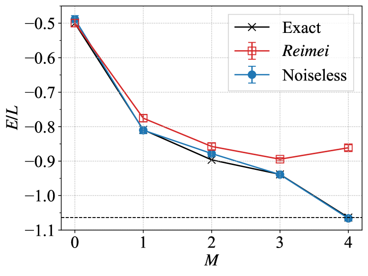
Figure 15: Energy per site as a function of the circuit depth $M$ for the 18-site lattice. Red squares represent the experimental results obtained using the Reimei system, blue circles denote the noiseless simulation results, and black crosses indicate the numerically exact results. The dashed horizontal line represents the exact ground-state energy of the final target Hamiltonian. The model parameters are the same as those used in Fig. 10.

Figure 16 shows the real and imaginary parts of $\langle\Psi_{M}(\bm{\theta}_{\rm opt})|\hat{\cal U}_{\rm R}|\Psi_{M}(\bm{\theta}_{\rm opt})\rangle$ as well as the associated polarization difference $\Delta{\cal P}_{\rm R}(M)$, evaluated in the same way as in Fig. 10 but using the Reimei system. Despite the significantly larger energy values compared to the exact results for $M=1,2,3,$ and $4$, the polarization evaluated with the Reimei system successfully captures the topological phase transition. These results support the robustness of the polarization against noise, attributed to its topological nature, as discussed in Sec. IV. It should be noted, however, that the energy and polarization experiments shown in Figs. 15 and 16, respectively, were performed independently.

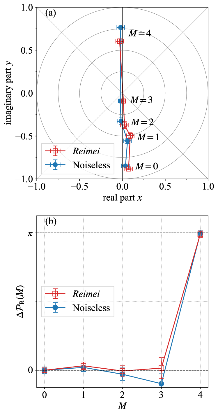
Figure 16: Same as Fig. 10, but the experimental results are obtained using the Reimei system.

References

- Feynman [1982] R. P. Feynman, Simulating physics with computers, International Journal of Theoretical Physics 21, 467 (1982).
- Lloyd [1996] S. Lloyd, Universal quantum simulators, Science 273, 1073 (1996), https://www.science.org/doi/pdf/10.1126/science.273.5278.1073 .
- Georgescu et al. [2014] I. M. Georgescu, S. Ashhab, and F. Nori, Quantum simulation, Rev. Mod. Phys. 86, 153 (2014).
- Mazurenko et al. [2017] A. Mazurenko, C. S. Chiu, G. Ji, M. F. Parsons, M. Kanász-Nagy, R. Schmidt, F. Grusdt, E. Demler, D. Greif, and M. Greiner, A cold-atom fermi–hubbard antiferromagnet, Nature 545, 462–466 (2017).
- Seki et al. [2020] K. Seki, T. Shirakawa, and S. Yunoki, Symmetry-adapted variational quantum eigensolver, Phys. Rev. A 101, 052340 (2020).
- Stanisic et al. [2022] S. Stanisic, J. L. Bosse, F. M. Gambetta, R. A. Santos, W. Mruczkiewicz, T. E. O’Brien, E. Ostby, and A. Montanaro, Observing ground-state properties of the fermi-hubbard model using a scalable algorithm on a quantum computer, Nature Communications 13, 10.1038/s41467-022-33335-4 (2022).
- Sun et al. [2023a] R.-Y. Sun, T. Shirakawa, and S. Yunoki, Efficient variational quantum circuit structure for correlated topological phases, Phys. Rev. B 108, 075127 (2023a).
- Kikuchi et al. [2023] Y. Kikuchi, C. Mc Keever, L. Coopmans, M. Lubasch, and M. Benedetti, Realization of quantum signal processing on a noisy quantum computer, npj Quantum Information 9, 10.1038/s41534-023-00762-0 (2023).
- Maskara et al. [2023] N. Maskara, S. Ostermann, J. Shee, M. Kalinowski, A. M. Gomez, R. A. Bravo, D. S. Wang, A. I. Krylov, N. Y. Yao, M. Head-Gordon, M. D. Lukin, and S. F. Yelin, Programmable simulations of molecules and materials with reconfigurable quantum processors (2023), arXiv:2312.02265 [quant-ph] .
- Summer et al. [2024] A. Summer, C. Chiaracane, M. T. Mitchison, and J. Goold, Calculating the many-body density of states on a digital quantum computer, Phys. Rev. Res. 6, 013106 (2024).
- Hémery et al. [2024] K. Hémery, K. Ghanem, E. Crane, S. L. Campbell, J. M. Dreiling, C. Figgatt, C. Foltz, J. P. Gaebler, J. Johansen, M. Mills, S. A. Moses, J. M. Pino, A. Ransford, M. Rowe, P. Siegfried, R. P. Stutz, H. Dreyer, A. Schuckert, and R. Nigmatullin, Measuring the loschmidt amplitude for finite-energy properties of the fermi-hubbard model on an ion-trap quantum computer, PRX Quantum 5, 030323 (2024).
- Seki et al. [2024] K. Seki, Y. Kikuchi, T. Hayata, and S. Yunoki, Simulating floquet scrambling circuits on trapped-ion quantum computers (2024), arXiv:2405.07613 [quant-ph] .
- Bañuls, Mari Carmen et al. [2020] Bañuls, Mari Carmen, Blatt, Rainer, Catani, Jacopo, Celi, Alessio, Cirac, Juan Ignacio, Dalmonte, Marcello, Fallani, Leonardo, Jansen, Karl, Lewenstein, Maciej, Montangero, Simone, Muschik, Christine A., Reznik, Benni, Rico, Enrique, Tagliacozzo, Luca, Van Acoleyen, Karel, Verstraete, Frank, Wiese, Uwe-Jens, Wingate, Matthew, Zakrzewski, Jakub, and Zoller, Peter, Simulating lattice gauge theories within quantum technologies, Eur. Phys. J. D 74, 165 (2020).
- Farrell et al. [2024] R. C. Farrell, M. Illa, A. N. Ciavarella, and M. J. Savage, Scalable circuits for preparing ground states on digital quantum computers: The schwinger model vacuum on 100 qubits, PRX Quantum 5, 020315 (2024).
- Hayata et al. [2024] T. Hayata, K. Seki, and A. Yamamoto, Floquet prethermalization of lattice gauge theory on superconducting qubits, Phys. Rev. D 110, 114503 (2024).
- Hayata and Hidaka [2025] T. Hayata and Y. Hidaka, Floquet evolution of the -deformed yang-mills theory on a two-leg ladder, Phys. Rev. D 111, 034513 (2025).
- Zhang et al. [2018] D.-W. Zhang, Y.-Q. Zhu, Y. X. Zhao, H. Yan, and S.-L. Z. and, Topological quantum matter with cold atoms, Advances in Physics 67, 253 (2018), https://doi.org/10.1080/00018732.2019.1594094 .
- Satzinger et al. [2021] K. J. Satzinger, Y.-J. Liu, A. Smith, C. Knapp, M. Newman, C. Jones, Z. Chen, C. Quintana, X. Mi, A. Dunsworth, C. Gidney, I. Aleiner, F. Arute, K. Arya, J. Atalaya, R. Babbush, J. C. Bardin, R. Barends, J. Basso, A. Bengtsson, A. Bilmes, M. Broughton, B. B. Buckley, D. A. Buell, B. Burkett, N. Bushnell, B. Chiaro, R. Collins, W. Courtney, S. Demura, A. R. Derk, D. Eppens, C. Erickson, L. Faoro, E. Farhi, A. G. Fowler, B. Foxen, M. Giustina, A. Greene, J. A. Gross, M. P. Harrigan, S. D. Harrington, J. Hilton, S. Hong, T. Huang, W. J. Huggins, L. B. Ioffe, S. V. Isakov, E. Jeffrey, Z. Jiang, D. Kafri, K. Kechedzhi, T. Khattar, S. Kim, P. V. Klimov, A. N. Korotkov, F. Kostritsa, D. Landhuis, P. Laptev, A. Locharla, E. Lucero, O. Martin, J. R. McClean, M. McEwen, K. C. Miao, M. Mohseni, S. Montazeri, W. Mruczkiewicz, J. Mutus, O. Naaman, M. Neeley, C. Neill, M. Y. Niu, T. E. O’Brien, A. Opremcak, B. Pató, A. Petukhov, N. C. Rubin, D. Sank, V. Shvarts, D. Strain, M. Szalay, B. Villalonga, T. C. White, Z. Yao, P. Yeh, J. Yoo, A. Zalcman, H. Neven, S. Boixo, A. Megrant, Y. Chen, J. Kelly, V. Smelyanskiy, A. Kitaev, M. Knap, F. Pollmann, and P. Roushan, Realizing topologically ordered states on a quantum processor, Science 374, 1237–1241 (2021).
- Smith et al. [2022] A. Smith, B. Jobst, A. G. Green, and F. Pollmann, Crossing a topological phase transition with a quantum computer, Phys. Rev. Res. 4, L022020 (2022).
- Moses et al. [2023] S. A. Moses, C. H. Baldwin, M. S. Allman, R. Ancona, L. Ascarrunz, C. Barnes, J. Bartolotta, B. Bjork, P. Blanchard, M. Bohn, J. G. Bohnet, N. C. Brown, N. Q. Burdick, W. C. Burton, S. L. Campbell, J. P. Campora, C. Carron, J. Chambers, J. W. Chan, Y. H. Chen, A. Chernoguzov, E. Chertkov, J. Colina, J. P. Curtis, R. Daniel, M. DeCross, D. Deen, C. Delaney, J. M. Dreiling, C. T. Ertsgaard, J. Esposito, B. Estey, M. Fabrikant, C. Figgatt, C. Foltz, M. Foss-Feig, D. Francois, J. P. Gaebler, T. M. Gatterman, C. N. Gilbreth, J. Giles, E. Glynn, A. Hall, A. M. Hankin, A. Hansen, D. Hayes, B. Higashi, I. M. Hoffman, B. Horning, J. J. Hout, R. Jacobs, J. Johansen, L. Jones, J. Karcz, T. Klein, P. Lauria, P. Lee, D. Liefer, S. T. Lu, D. Lucchetti, C. Lytle, A. Malm, M. Matheny, B. Mathewson, K. Mayer, D. B. Miller, M. Mills, B. Neyenhuis, L. Nugent, S. Olson, J. Parks, G. N. Price, Z. Price, M. Pugh, A. Ransford, A. P. Reed, C. Roman, M. Rowe, C. Ryan-Anderson, S. Sanders, J. Sedlacek, P. Shevchuk, P. Siegfried, T. Skripka, B. Spaun, R. T. Sprenkle, R. P. Stutz, M. Swallows, R. I. Tobey, A. Tran, T. Tran, E. Vogt, C. Volin, J. Walker, A. M. Zolot, and J. M. Pino, A race-track trapped-ion quantum processor, Phys. Rev. X 13, 041052 (2023).
- McKay et al. [2023] D. C. McKay, I. Hincks, E. J. Pritchett, M. Carroll, L. C. G. Govia, and S. T. Merkel, Benchmarking quantum processor performance at scale (2023), arXiv:2311.05933 [quant-ph] .
- Bluvstein et al. [2023] D. Bluvstein, S. J. Evered, A. A. Geim, S. H. Li, H. Zhou, T. Manovitz, S. Ebadi, M. Cain, M. Kalinowski, D. Hangleiter, J. P. Bonilla Ataides, N. Maskara, I. Cong, X. Gao, P. Sales Rodriguez, T. Karolyshyn, G. Semeghini, M. J. Gullans, M. Greiner, V. Vuletić, and M. D. Lukin, Logical quantum processor based on reconfigurable atom arrays, Nature 626, 58–65 (2023).
- Sunada et al. [2024] Y. Sunada, K. Yuki, Z. Wang, T. Miyamura, J. Ilves, K. Matsuura, P. A. Spring, S. Tamate, S. Kono, and Y. Nakamura, Photon-noise-tolerant dispersive readout of a superconducting qubit using a nonlinear purcell filter, PRX Quantum 5, 010307 (2024).
- Li et al. [2024] R. Li, K. Kubo, Y. Ho, Z. Yan, Y. Nakamura, and H. Goto, Realization of high-fidelity cz gate based on a double-transmon coupler, Phys. Rev. X 14, 041050 (2024).
- Gao et al. [2024] D. Gao, D. Fan, C. Zha, J. Bei, G. Cai, J. Cai, S. Cao, X. Zeng, F. Chen, J. Chen, K. Chen, X. Chen, X. Chen, Z. Chen, Z. Chen, Z. Chen, W. Chu, H. Deng, Z. Deng, P. Ding, X. Ding, Z. Ding, S. Dong, Y. Dong, B. Fan, Y. Fu, S. Gao, L. Ge, M. Gong, J. Gui, C. Guo, S. Guo, X. Guo, T. He, L. Hong, Y. Hu, H.-L. Huang, Y.-H. Huo, T. Jiang, Z. Jiang, H. Jin, Y. Leng, D. Li, D. Li, F. Li, J. Li, J. Li, J. Li, J. Li, N. Li, S. Li, W. Li, Y. Li, Y. Li, F. Liang, X. Liang, N. Liao, J. Lin, W. Lin, D. Liu, H. Liu, M. Liu, X. Liu, X. Liu, Y. Liu, H. Lou, Y. Ma, L. Meng, H. Mou, K. Nan, B. Nie, M. Nie, J. Ning, L. Niu, W. Peng, H. Qian, H. Rong, T. Rong, H. Shen, Q. Shen, H. Su, F. Su, C. Sun, L. Sun, T. Sun, Y. Sun, Y. Tan, J. Tan, L. Tang, W. Tu, C. Wan, J. Wang, B. Wang, C. Wang, C. Wang, C. Wang, J. Wang, L. Wang, R. Wang, S. Wang, X. Wang, Z. Wei, J. Wei, D. Wu, G. Wu, J. Wu, S. Wu, Y. Wu, S. Xie, L. Xin, Y. Xu, C. Xue, K. Yan, W. Yang, X. Yang, Y. Yang, Y. Ye, Z. Ye, C. Ying, J. Yu, Q. Yu, W. Yu, S. Zhan, F. Zhang, H. Zhang, K. Zhang, P. Zhang, W. Zhang, Y. Zhang, Y. Zhang, L. Zhang, G. Zhao, P. Zhao, X. Zhao, X. Zhao, Y. Zhao, Z. Zhao, L. Zheng, F. Zhou, L. Zhou, N. Zhou, N. Zhou, S. Zhou, S. Zhou, Z. Zhou, C. Zhu, Q. Zhu, G. Zou, H. Zou, Q. Zhang, C.-Y. Lu, C.-Z. Peng, X. Zhu, and J.-W. Pan, Establishing a new benchmark in quantum computational advantage with 105-qubit zuchongzhi 3.0 processor (2024), arXiv:2412.11924 [quant-ph] .
- Preskill [2018] J. Preskill, Quantum Computing in the NISQ era and beyond, Quantum 2, 79 (2018).
- Arute et al. [2019] F. Arute, K. Arya, R. Babbush, D. Bacon, J. C. Bardin, R. Barends, R. Biswas, S. Boixo, F. G. S. L. Brandao, D. A. Buell, B. Burkett, Y. Chen, Z. Chen, B. Chiaro, R. Collins, W. Courtney, A. Dunsworth, E. Farhi, B. Foxen, A. Fowler, C. Gidney, M. Giustina, R. Graff, K. Guerin, S. Habegger, M. P. Harrigan, M. J. Hartmann, A. Ho, M. Hoffmann, T. Huang, T. S. Humble, S. V. Isakov, E. Jeffrey, Z. Jiang, D. Kafri, K. Kechedzhi, J. Kelly, P. V. Klimov, S. Knysh, A. Korotkov, F. Kostritsa, D. Landhuis, M. Lindmark, E. Lucero, D. Lyakh, S. Mandrà, J. R. McClean, M. McEwen, A. Megrant, X. Mi, K. Michielsen, M. Mohseni, J. Mutus, O. Naaman, M. Neeley, C. Neill, M. Y. Niu, E. Ostby, A. Petukhov, J. C. Platt, C. Quintana, E. G. Rieffel, P. Roushan, N. C. Rubin, D. Sank, K. J. Satzinger, V. Smelyanskiy, K. J. Sung, M. D. Trevithick, A. Vainsencher, B. Villalonga, T. White, Z. J. Yao, P. Yeh, A. Zalcman, H. Neven, and J. M. Martinis, Quantum supremacy using a programmable superconducting processor, Nature 574, 505 (2019).
- Zhong et al. [2020] H.-S. Zhong, H. Wang, Y.-H. Deng, M.-C. Chen, L.-C. Peng, Y.-H. Luo, J. Qin, D. Wu, X. Ding, Y. Hu, P. Hu, X.-Y. Yang, W.-J. Zhang, H. Li, Y. Li, X. Jiang, L. Gan, G. Yang, L. You, Z. Wang, L. Li, N.-L. Liu, C.-Y. Lu, and J.-W. Pan, Quantum computational advantage using photons, Science 370, 1460 (2020), https://www.science.org/doi/pdf/10.1126/science.abe8770 .
- Wu et al. [2021] Y. Wu, W.-S. Bao, S. Cao, F. Chen, M.-C. Chen, X. Chen, T.-H. Chung, H. Deng, Y. Du, D. Fan, M. Gong, C. Guo, C. Guo, S. Guo, L. Han, L. Hong, H.-L. Huang, Y.-H. Huo, L. Li, N. Li, S. Li, Y. Li, F. Liang, C. Lin, J. Lin, H. Qian, D. Qiao, H. Rong, H. Su, L. Sun, L. Wang, S. Wang, D. Wu, Y. Xu, K. Yan, W. Yang, Y. Yang, Y. Ye, J. Yin, C. Ying, J. Yu, C. Zha, C. Zhang, H. Zhang, K. Zhang, Y. Zhang, H. Zhao, Y. Zhao, L. Zhou, Q. Zhu, C.-Y. Lu, C.-Z. Peng, X. Zhu, and J.-W. Pan, Strong quantum computational advantage using a superconducting quantum processor, Phys. Rev. Lett. 127, 180501 (2021).
- Zhong et al. [2021] H.-S. Zhong, Y.-H. Deng, J. Qin, H. Wang, M.-C. Chen, L.-C. Peng, Y.-H. Luo, D. Wu, S.-Q. Gong, H. Su, Y. Hu, P. Hu, X.-Y. Yang, W.-J. Zhang, H. Li, Y. Li, X. Jiang, L. Gan, G. Yang, L. You, Z. Wang, L. Li, N.-L. Liu, J. J. Renema, C.-Y. Lu, and J.-W. Pan, Phase-programmable gaussian boson sampling using stimulated squeezed light, Phys. Rev. Lett. 127, 180502 (2021).
- Morvan et al. [2024] A. Morvan, B. Villalonga, X. Mi, S. Mandrà, A. Bengtsson, P. V. Klimov, Z. Chen, S. Hong, C. Erickson, I. K. Drozdov, J. Chau, G. Laun, R. Movassagh, A. Asfaw, L. T. A. N. Brandão, R. Peralta, D. Abanin, R. Acharya, R. Allen, T. I. Andersen, K. Anderson, M. Ansmann, F. Arute, K. Arya, J. Atalaya, J. C. Bardin, A. Bilmes, G. Bortoli, A. Bourassa, J. Bovaird, L. Brill, M. Broughton, B. B. Buckley, D. A. Buell, T. Burger, B. Burkett, N. Bushnell, J. Campero, H.-S. Chang, B. Chiaro, D. Chik, C. Chou, J. Cogan, R. Collins, P. Conner, W. Courtney, A. L. Crook, B. Curtin, D. M. Debroy, A. D. T. Barba, S. Demura, A. D. Paolo, A. Dunsworth, L. Faoro, E. Farhi, R. Fatemi, V. S. Ferreira, L. F. Burgos, E. Forati, A. G. Fowler, B. Foxen, G. Garcia, É. Genois, W. Giang, C. Gidney, D. Gilboa, M. Giustina, R. Gosula, A. G. Dau, J. A. Gross, S. Habegger, M. C. Hamilton, M. Hansen, M. P. Harrigan, S. D. Harrington, P. Heu, M. R. Hoffmann, T. Huang, A. Huff, W. J. Huggins, L. B. Ioffe, S. V. Isakov, J. Iveland, E. Jeffrey, Z. Jiang, C. Jones, P. Juhas, D. Kafri, T. Khattar, M. Khezri, M. Kieferová, S. Kim, A. Kitaev, A. R. Klots, A. N. Korotkov, F. Kostritsa, J. M. Kreikebaum, D. Landhuis, P. Laptev, K.-M. Lau, L. Laws, J. Lee, K. W. Lee, Y. D. Lensky, B. J. Lester, A. T. Lill, W. Liu, W. P. Livingston, A. Locharla, F. D. Malone, O. Martin, S. Martin, J. R. McClean, M. McEwen, K. C. Miao, A. Mieszala, S. Montazeri, W. Mruczkiewicz, O. Naaman, M. Neeley, C. Neill, A. Nersisyan, M. Newman, J. H. Ng, A. Nguyen, M. Nguyen, M. Y. Niu, T. E. O’Brien, S. Omonije, A. Opremcak, A. Petukhov, R. Potter, L. P. Pryadko, C. Quintana, D. M. Rhodes, C. Rocque, E. Rosenberg, N. C. Rubin, N. Saei, D. Sank, K. Sankaragomathi, K. J. Satzinger, H. F. Schurkus, C. Schuster, M. J. Shearn, A. Shorter, N. Shutty, V. Shvarts, V. Sivak, J. Skruzny, W. C. Smith, R. D. Somma, G. Sterling, D. Strain, M. Szalay, D. Thor, A. Torres, G. Vidal, C. V. Heidweiller, T. White, B. W. K. Woo, C. Xing, Z. J. Yao, P. Yeh, J. Yoo, G. Young, A. Zalcman, Y. Zhang, N. Zhu, N. Zobrist, E. G. Rieffel, R. Biswas, R. Babbush, D. Bacon, J. Hilton, E. Lucero, H. Neven, A. Megrant, J. Kelly, P. Roushan, I. Aleiner, V. Smelyanskiy, K. Kechedzhi, Y. Chen, and S. Boixo, Phase transitions in random circuit sampling, Nature 634, 328 (2024).
- DeCross et al. [2024] M. DeCross, R. Haghshenas, M. Liu, E. Rinaldi, J. Gray, Y. Alexeev, C. H. Baldwin, J. P. Bartolotta, M. Bohn, E. Chertkov, J. Cline, J. Colina, D. DelVento, J. M. Dreiling, C. Foltz, J. P. Gaebler, T. M. Gatterman, C. N. Gilbreth, J. Giles, D. Gresh, A. Hall, A. Hankin, A. Hansen, N. Hewitt, I. Hoffman, C. Holliman, R. B. Hutson, T. Jacobs, J. Johansen, P. J. Lee, E. Lehman, D. Lucchetti, D. Lykov, I. S. Madjarov, B. Mathewson, K. Mayer, M. Mills, P. Niroula, J. M. Pino, C. Roman, M. Schecter, P. E. Siegfried, B. G. Tiemann, C. Volin, J. Walker, R. Shaydulin, M. Pistoia, S. A. Moses, D. Hayes, B. Neyenhuis, R. P. Stutz, and M. Foss-Feig, The computational power of random quantum circuits in arbitrary geometries (2024), arXiv:2406.02501 [quant-ph] .
- Kim et al. [2023] Y. Kim, A. Eddins, S. Anand, K. X. Wei, E. van den Berg, S. Rosenblatt, H. Nayfeh, Y. Wu, M. Zaletel, K. Temme, and A. Kandala, Evidence for the utility of quantum computing before fault tolerance, Nature 618, 500 (2023).
- Alexeev et al. [2024] Y. Alexeev, M. Amsler, M. A. Barroca, S. Bassini, T. Battelle, D. Camps, D. Casanova, Y. J. Choi, F. T. Chong, C. Chung, C. Codella, A. D. Córcoles, J. Cruise, A. Di Meglio, I. Duran, T. Eckl, S. Economou, S. Eidenbenz, B. Elmegreen, C. Fare, I. Faro, C. S. Fernández, R. N. B. Ferreira, K. Fuji, B. Fuller, L. Gagliardi, G. Galli, J. R. Glick, I. Gobbi, P. Gokhale, S. de la Puente Gonzalez, J. Greiner, B. Gropp, M. Grossi, E. Gull, B. Healy, M. R. Hermes, B. Huang, T. S. Humble, N. Ito, A. F. Izmaylov, A. Javadi-Abhari, D. Jennewein, S. Jha, L. Jiang, B. Jones, W. A. de Jong, P. Jurcevic, W. Kirby, S. Kister, M. Kitagawa, J. Klassen, K. Klymko, K. Koh, M. Kondo, D. M. Kürkçüog̃lu, K. Kurowski, T. Laino, R. Landfield, M. Leininger, V. Leyton-Ortega, A. Li, M. Lin, J. Liu, N. Lorente, A. Luckow, S. Martiel, F. Martin-Fernandez, M. Martonosi, C. Marvinney, A. C. Medina, D. Merten, A. Mezzacapo, K. Michielsen, A. Mitra, T. Mittal, K. Moon, J. Moore, S. Mostame, M. Motta, Y.-H. Na, Y. Nam, P. Narang, Y.-y. Ohnishi, D. Ottaviani, M. Otten, S. Pakin, V. R. Pascuzzi, E. Pednault, T. Piontek, J. Pitera, P. Rall, G. S. Ravi, N. Robertson, M. A. Rossi, P. Rydlichowski, H. Ryu, G. Samsonidze, M. Sato, N. Saurabh, V. Sharma, K. Sharma, S. Shin, G. Slessman, M. Steiner, I. Sitdikov, I.-S. Suh, E. D. Switzer, W. Tang, J. Thompson, S. Todo, M. C. Tran, D. Trenev, C. Trott, H.-H. Tseng, N. M. Tubman, E. Tureci, D. G. Valiñas, S. Vallecorsa, C. Wever, K. Wojciechowski, X. Wu, S. Yoo, N. Yoshioka, V. W.-z. Yu, S. Yunoki, S. Zhuk, and D. Zubarev, Quantum-centric supercomputing for materials science: A perspective on challenges and future directions, Future Generation Computer Systems 160, 666 (2024).
- Shinjo et al. [2024] K. Shinjo, K. Seki, T. Shirakawa, R.-Y. Sun, and S. Yunoki, Unveiling clean two-dimensional discrete time quasicrystals on a digital quantum computer, arXiv e-prints , arXiv:2403.16718 (2024), arXiv:2403.16718 [quant-ph] .
- Robledo-Moreno et al. [2024] J. Robledo-Moreno, M. Motta, H. Haas, A. Javadi-Abhari, P. Jurcevic, W. Kirby, S. Martiel, K. Sharma, S. Sharma, T. Shirakawa, I. Sitdikov, R.-Y. Sun, K. J. Sung, M. Takita, M. C. Tran, S. Yunoki, and A. Mezzacapo, Chemistry Beyond Exact Solutions on a Quantum-Centric Supercomputer, arXiv e-prints , arXiv:2405.05068 (2024), arXiv:2405.05068 [quant-ph] .
- Peruzzo et al. [2014] A. Peruzzo, J. McClean, P. Shadbolt, M.-H. Yung, X.-Q. Zhou, P. J. Love, A. Aspuru-Guzik, and J. L. O’Brien, A variational eigenvalue solver on a photonic quantum processor, Nature Communications 5, 10.1038/ncomms5213 (2014).
- Kandala et al. [2017] A. Kandala, A. Mezzacapo, K. Temme, M. Takita, M. Brink, J. M. Chow, and J. M. Gambetta, Hardware-efficient variational quantum eigensolver for small molecules and quantum magnets, Nature 549, 242–246 (2017).
- Farhi et al. [2014] E. Farhi, J. Goldstone, and S. Gutmann, A Quantum Approximate Optimization Algorithm, arXiv e-prints , arXiv:1411.4028 (2014), arXiv:1411.4028 [quant-ph] .
- Seki and Yunoki [2022] K. Seki and S. Yunoki, Spatial, spin, and charge symmetry projections for a fermi-hubbard model on a quantum computer, Phys. Rev. A 105, 032419 (2022).
- Sun et al. [2023b] R.-Y. Sun, T. Shirakawa, and S. Yunoki, Parametrized quantum circuit for weight-adjustable quantum loop gas, Physical Review B 107, 10.1103/physrevb.107.l041109 (2023b).
- McClean et al. [2018] J. R. McClean, S. Boixo, V. N. Smelyanskiy, R. Babbush, and H. Neven, Barren plateaus in quantum neural network training landscapes, Nature Communications 9, 4812 (2018).
- Shirakawa et al. [2021] T. Shirakawa, K. Seki, and S. Yunoki, Discretized quantum adiabatic process for free fermions and comparison with the imaginary-time evolution, Phys. Rev. Research 3, 013004 (2021).
- Su et al. [1979] W. P. Su, J. R. Schrieffer, and A. J. Heeger, Solitons in polyacetylene, Phys. Rev. Lett. 42, 1698 (1979).
- Asbóth et al. [2015] J. K. Asbóth, L. Oroszlány, and A. Pályi, A Short Course on Topological Insulators: Band-structure topology and edge states in one and two dimensions, arXiv e-prints , arXiv:1509.02295 (2015), arXiv:1509.02295 [cond-mat.mes-hall] .
- [46] System Model H1 Powered by Honeywell, accessed on January 18th, 2024.
- Resta [1998] R. Resta, Quantum-mechanical position operator in extended systems, Phys. Rev. Lett. 80, 1800 (1998).
- Jordan and Wigner [1928] P. Jordan and E. Wigner, Über das paulische äquivalenzverbot, Zeitschrift für Physik 47, 631 (1928).
- Bravyi and Kitaev [2002] S. B. Bravyi and A. Y. Kitaev, Fermionic quantum computation, Annals of Physics 298, 210 (2002).
- Ball [2005] R. C. Ball, Fermions without fermion fields, Phys. Rev. Lett. 95, 176407 (2005).
- Verstraete and Cirac [2005] F. Verstraete and J. I. Cirac, Mapping local hamiltonians of fermions to local hamiltonians of spins, Journal of Statistical Mechanics: Theory and Experiment 2005, P09012 (2005).
- Ruh et al. [2022] J. Ruh, R. Finsterhoelzl, and G. Burkard, Digital quantum simulation of the bcs model with a central-spin-like quantum processor, arXiv e-prints , arXiv:2209.09225 (2022), arXiv:2209.09225 [quant-ph] .
- Steudtner and Wehner [2018] M. Steudtner and S. Wehner, Fermion-to-qubit mappings with varying resource requirements for quantum simulation, New Journal of Physics 20, 063010 (2018).
- Jiang et al. [2020] Z. Jiang, A. Kalev, W. Mruczkiewicz, and H. Neven, Optimal fermion-to-qubit mapping via ternary trees with applications to reduced quantum states learning, Quantum 4, 276 (2020).
- Chen and Xu [2023] Y.-A. Chen and Y. Xu, Equivalence between fermion-to-qubit mappings in two spatial dimensions, PRX Quantum 4, 010326 (2023).
- Nys and Carleo [2023] J. Nys and G. Carleo, Quantum circuits for solving local fermion-to-qubit mappings, Quantum 7, 930 (2023).
- Lieb and Robinson [1972] E. H. Lieb and D. W. Robinson, The finite group velocity of quantum spin systems, Communications in Mathematical Physics 28, 251 (1972).
- Jobst et al. [2022] B. Jobst, A. Smith, and F. Pollmann, Finite-depth scaling of infinite quantum circuits for quantum critical points, Phys. Rev. Res. 4, 033118 (2022).
- Calabrese and Cardy [2004] P. Calabrese and J. Cardy, Entanglement entropy and quantum field theory, Journal of Statistical Mechanics: Theory and Experiment 2004, P06002 (2004).
- Watanabe and Oshikawa [2018] H. Watanabe and M. Oshikawa, Inequivalent berry phases for the bulk polarization, Phys. Rev. X 8, 021065 (2018).
- Sivarajah et al. [2020] S. Sivarajah, S. Dilkes, A. Cowtan, W. Simmons, A. Edgington, and R. Duncan, t—ket⟩: a retargetable compiler for nisq devices, Quantum Science and Technology 6, 014003 (2020).
- Hohenadler and Assaad [2013] M. Hohenadler and F. F. Assaad, Correlation effects in two-dimensional topological insulators, Journal of Physics: Condensed Matter 25, 143201 (2013).
- Rachel [2018] S. Rachel, Interacting topological insulators: a review, Reports on Progress in Physics 81, 116501 (2018).
- Bigan Mbeng et al. [2019] G. Bigan Mbeng, R. Fazio, and G. E. Santoro, Optimal quantum control with digitized quantum annealing, arXiv e-prints , arXiv:1911.12259 (2019), arXiv:1911.12259 [quant-ph] .
- [65] https://github.com/CQCL/quantinuum-hardware-specifications/blob/main/notebooks, accessed on March 26th, 2025.