Satellite System Architecting Considering On-Orbit Refueling

Abstract

This paper introduces the problem of selecting a satellite system architecture considering commercial on-orbit refueling (OOR). The problem aims to answer two questions: “How durable should a satellite be?” and “How much propellant should be loaded into the satellite at launch?” We formulate the problem as a mathematical optimization by adopting the design lifetime and propellant mass as design variables and considering two objective functions to balance the returns and risks. A surrogate model-based framework, grounded in a satellite lifecycle simulation, is developed to address this problem. The developed framework considers various uncertainties and operational flexibility and integrates a modified satellite sizing and cost model by adjusting traditional models with OOR. A design case study of a geosynchronous equatorial orbit communication satellite considering the OOR highlights the effectiveness of the developed framework.

Nomenclature

$a_{\text{prop}},b_{\text{prop}}$  =	coefficients for propulsion subsystem mass, kg1/3, kg
$C_{\text{IOC}}$  =	initial operational capability cost, $M
$C_{\text{lau}}$  =	launch cost, $M
$C_{\text{oor}}$  =	On-Orbit Refueling (OOR) service cost, $M
$C_{\text{op}}$  =	satellite operational cost, $M
$C_{\text{sat}}$  =	satellite acquisition cost, $M
$c_{\text{lau}}$  =	specific launch cost, $M/kg
$c_{f,\text{oor}}$  =	fixed cost of OOR service, $M
$c_{v,\text{oor}}$  =	variable cost coefficient of OOR service, $M/kg
$c_{\text{sat}}$  =	specific satellite acquisition cost, $M/kg
$\mathcal{H}$  =	half-normal distribution with zero as the lower bound
$I_{\text{sp}}$  =	specific impulse of the propulsion subsystem, sec
$M_{\text{oor}}$  =	OOR service capacity, kg
$m_{\text{adcs}}$  =	attitude determination and control subsystem mass of a satellite, kg
$m_{\text{base}}$  =	base mass of a satellite, kg
$m_{\text{dry}}$  =	dry mass of a satellite, kg
$m_{\text{ps}}$  =	propulsion subsystem mass of a satellite, kg
$m_{\text{ref}}$  =	reference mass, kg
$m_{\text{serv}}$  =	servicing interface mass of a satellite, kg
$m_{\text{str}}$  =	structure mass of a satellite, kg
$m_{\text{wet}}$  =	wet mass of a satellite, kg
$m_{p,\text{des}}$  =	design propellant mass of a satellite, kg
$m_{p,\text{ioa}}$  =	propellant mass required for initial orbit acquisition, kg
$m_{p,\text{oor}}$  =	propellant amount to be replenished, kg
$p_{f,\text{lau}}$  =	launch failure rate
$p_{f,\text{oor}}$  =	OOR service failure rate
$r_{\text{adcs}}$  =	attitude determination and control subsystem mass ratio
$r_{f}$  =	risk free rate
$r_{\text{ins}}$  =	insurance cost ratio
$r_{\text{op}}$  =	operational cost ratio
$r_{\text{str}}$  =	structural mass ratio
$r_{\text{serv}}$  =	servicing interface mass ratio
$R$  =	satellite operational revenue, $M/yr
$R_{0}$  =	initial operational revenue, $M/yr
$Rel$  =	reliability function of a satellite
$Rel_{\text{ref}}$  =	reliability function of a satellite with the reference design lifetime
$T$  =	time in continuous frame, yr
$t$  =	time in discretized frame ($=T/\Delta T$)
$\Delta T$  =	time step size in year, yr
$T_{\text{life}}$, $t_{\text{life}}$  =	design lifetime of satellite in year and time step, yr, -
$T_{\text{obs}}$  =	parameter for technology obsolescence, yr
$T_{r,\text{oor}}$, $t_{r,\text{oor}}$  =	time to OOR service in year and time step, yr, -
$T_{\text{ref}}$  =	reference design lifetime, yr
$T_{r,\text{rep}}$, $t_{r,\text{rep}}$  =	time to replacement in year and time step, yr, -
$T_{\text{sim}}$, $t_{\text{sim}}$  =	simulation time in year and time step, yr, -
$\Delta V_{\text{err}}$  =	$\Delta V$ required for correcting the injection error of the launch vehicle, m/s
$\Delta V_{\text{ioa}}$  =	$\Delta V$ required for initial orbit acquisition, m/s
$\Delta V_{\text{ot}}$, $\Delta V_{\text{ot},\text{ideal}}$  =	real and ideal $\Delta V$ required for transferring from the initial orbit to the target orbit, m/s, m/s
$\Delta V_{\text{stk},\text{yr}}$  =	Annual $\Delta V$ requirement for station-keeping, m/s
$\Delta v_{\text{stk}}$  =	$\Delta V$ requirement for station-keeping per time step, m/s
$\alpha,\beta_{1},\beta_{2},\theta_{1},\theta_{2}$  =	parameters for reliability function, -, -, -, yr, yr
$\Phi$  =	cumulative distribution function of the standard normal distribution
$\phi_{\text{mar}}$  =	market volatility factor in operational revenue
$\phi_{\text{obs}}$  =	technology obsolescence factor in operational revenue
$\sigma_{\text{mar}}$  =	market volatility, yr-1/2
$\sigma_{\text{oi}}$  =	parameter of $\Delta V$ distribution for correcting orbit injection error
$\mu_{\text{mar}}$  =	market drift rate, yr-1
$\kappa$  =	mass growth rate of a satellite to the design lifetime

1 Introduction

SPACE systems remain among the most expensive and complex, even in this era of abundant advanced technologies. However, only a limited number of these systems, such as the International Space Station and the Hubble Space Telescope, have benefited from post-launch servicing (e.g., maintenance, repair, or replenishment)—a routine practice for complex ground systems. The primary reasons for this limitation are the high costs and risks associated with human-involved on-orbit servicing (OOS) activities and the expenses of launches. Consequently, most space systems are equipped with all the necessary resources for their entire operation at launch. This approach, while necessary, has exacerbated the impact of failures, thereby placing a premium on system reliability. The increased focus on reliability and the significant price of launch vehicles have led to escalating expenses and complexity in satellite systems. This trend, characteristic of the risk-averse space industry, has contributed to the gradual extension of the design lifetimes of space systems.

However, the space sector is undergoing a significant transformation with the emergence of new commercial entities. These entities are driven by advancements in launch vehicle technologies, which have significantly reduced launch costs, fostering innovative concepts that enhance the value of space systems. A notable innovation is the on-orbit refueling (OOR), a subset of OOS [1, 2, 3, 4]. This innovation, supported by advancements in robotics, autonomous control, and servicing architecture design, primarily serves as a life-extension solution for existing assets of substantial value, such as the geosynchronous equatorial orbit (GEO) communication satellites. This approach does not require significant modifications to existing design and operational paradigms. Instead, it introduces supplementary procedures after the depletion of the initial propellant load, promising profitability through the extended utility of these satellites. Consequently, the commercialization of OOR appears imminent as stakeholders in the space industry seek to capitalize on its potential. For example, Orbit Fab plans to provide in-orbit hydrazine for GEO satellites weighing up to 100 kilograms at a cost of $25 million by 2025 [5].

On the other hand, OOR also introduces significant changes to satellite system design—the separation of the design lifetime and the design propellant mass of a satellite. Traditionally, a satellite intended for a 15-year mission carries all the propellant needed throughout its mission duration. However, with the OOR, satellites can carry a smaller initial propellant amount and rely on the refueling service in the future. This raises a question about the traditional approach: “Will it remain the best option to load all the propellant required for the lifetime at launch?” If not, “How much propellant should be equipped at launch, and when should the propellant be refilled?” These questions lead to studying the potential of architectural changes, which is essential not only for the profitability of the players in the market but also for the long-term sustainability of the overall space industry [6]. Answering these questions requires consideration of the satellite’s behavior, environmental interactions, and how these factors influence its overall value and performance. A comprehensive evaluation of the satellite’s entire lifecycle is essential to analyze this dynamic and make optimal decisions.

The design lifetime of a system—the period during which the system operates as intended—appears as a requirement and derives other lower-level requirements, such as the reliability of each subsystem and the amount of each consumable. The satellite’s design lifetime has been a research topic as a crucial element of satellite architecture. Saleh et al. [7] analyzed the impact of the satellite design lifetime on the sizing and cost of satellites and provided models for these as functions of the design lifetime. A key finding from this study is the quantified increase in total mass for GEO communication satellites, estimated at approximately 3% for each additional year of design lifetime from 3 years of design lifetime. This observation has become a foundational reference in subsequent studies that analyze system architecture of space systems.

In a commercial context, economic considerations profoundly influence the decision-making process regarding spacecraft design lifetime, as explored in a series of papers [8, 9, 10]. These studies investigated how design lifetime affects the value of satellite systems by considering environmental factors (e.g., market and technological advancements) from multiple perspectives—including those of satellite operators, manufacturers, society, and customers. Overall, the studies imply that as situations become increasingly competitive and uncertain, a simplistic, cost-driven approach leads to misguided solutions that expose stakeholders to greater risks.

In addition to these advancements in analyzing the economic implications of satellite design lifetime, the value analysis of OOS in space systems has been extensively studied since the 1970s. The research group led by Dr. Hastings is a significant contributor to this field. They focused on the strategic advantage of flexibility provided by OOS, employing quantitative approaches to analyze its value in various OOS scenarios. Their extensive work, especially in the 2000s, is well-documented in various journal articles [11, 12, 13, 14, 15] and theses [16, 17, 18, 19, 20], offering a comprehensive view of the strategic implications and benefits of OOS. A key contribution of these works is the incorporation of the operational flexibility provided by OOS into the evaluation framework through various techniques (e.g., decision tree analysis and real options [21]). Using these techniques, the authors investigated the value offered by different OOS types—such as life-extension and upgrades—and examined how OOS could lead to changes in satellite system architecture, specifically in the design lifetime of a satellite

Recognizing the flexibility OOS provides has prompted extensive research into its value across various operational scenarios, employing diverse methodologies. For example, Yao et al. [22] approached OOS from a design optimization perspective, considering both service providers and clients. Their methodology factored in design lifetime, life-extension length, number of servicing operations before refueling, and the orbit radii of parking and depots. They utilized probability and evidence theories to address uncertainties in the operational environment. The study employed dynamic programming to select the optimal servicing activity based on modeled uncertainties. The authors decomposed the optimization problem into sub-problems to manage the computational complexity, enabling efficient analysis of a hypothetical GEO communication satellite case.

More recently, Liu et al. [23] focused on the economic aspects of OOS, using the MEV-1 mission [24] as a case study. They developed a high-fidelity cost-and-benefit model, incorporating insurance, taxes, depreciation, and other realistic economic parameters. Their analysis revealed that the MEV-1’s service pricing was at the lower end of the feasible range, likely to attract customers in a nascent market. They also suggested that the distribution of value and risk associated with OOS will be crucial for the future space industry.

Building on these academic efforts, we introduce a new problem in satellite system architecting. In this problem, we decouple the design lifetime from the propellant mass to account for an expanded range of satellite system architectural solutions that OOR commercialization drives—a perspective not covered in existing works. To address this problem while accommodating operational flexibility and various uncertainties, we propose a satellite lifecycle simulation for evaluating each architectural solution and introduce a solution procedure assisted by surrogate models.

The rest of this paper is organized into five sections. Section II delineates the decision-making problem of interest and provides its mathematical representation. Section III introduces the satellite lifecycle simulation, which forms the baseline for the solution procedure. Section IV details the solution procedure based on this simulation assisted by surrogate models. Section V presents a case study to validate the developed framework and offers meaningful insights. Finally, Section VI concludes the paper, summarizing its contents and contributions and proposing future works.

2 Problem Description

In a traditional approach, the design lifetime of a satellite, which is constrained by the planned operational time and technological factors, primarily influences its design propellant mass. Consider, for instance, a GEO communication satellite intended for a 15-year operational period. In such cases, the satellite is launched with enough propellant to support all the projected maneuvers during its mission. This covers initial orbit insertion errors and station-keeping maneuvers, which typically require a $\Delta V$ of around 50 m/s annually. Within this design scheme, the designer’s choice of propellant mass is highly constrained. Without additional supply strategy except the initial loading, the degree of conservatism becomes the only variable under the designer’s control. This degree of conservatism typically appears in the design as a margin, providing a buffer to ensure mission success under potential deviations in mission environments.

However, while this traditional approach is time-tested, it limits the design space of satellites in the context of OOR. OOR introduces a paradigm shift by allowing propellant replenishment after launch, expanding the design space beyond those dictated solely by the loaded propellant at launch. In this new context, the propellant mass is no longer solely tied to the spacecraft’s design lifetime. Instead, it becomes an independent variable determined by a comprehensive assessment of how it impacts the overall system value. This change enables a more adaptable satellite system architecture, potentially enhancing the system’s value. A careful approach is essential in the initial design phase for the designer to realize this potential.

This approach involves the trade-off between efficiency improvement and complexity increase. On the one hand, reducing the initial propellant mass leads to a smaller tank than traditional designs, decreasing the satellite’s overall structural mass. This reduction may relax the performance requirement on actuators such as reaction wheels, potentially reducing overall mission costs, including development, manufacturing, and launch costs. Additionally, the reduced overall expenditure on system acquisition mitigates loss in mission failures. On the other hand, integrating OOR into the satellite’s operational scenario introduces new complexities. This integration not only incurs additional servicing costs and introduces a potential new source of failure but also requires accommodating the service interface for OOR, which increases the satellite’s size. The cumulative effect of these factors could offset the benefits derived from reduced propellant mass. Consequently, while OOR offers opportunities for cost reduction and increased flexibility, it also presents challenges that necessitate cautious management during the initial design phase.

A well-structured methodology grounded in quantitative analysis is essential to analyze these trade-offs and derive an efficient solution systematically. For this purpose, this research mathematically encodes this decision-making context into an optimization problem. The design variables include a satellite’s design lifetime and propellant mass. Each choice of design variables reflects the designer’s intention about “how long the system should operate” and “how much propellant is to be loaded at launch,” with each combination indicating a distinct design solution.

The optimal choice of the design variables varies according to the system value metric defined by its stakeholders. One possible approach is the monetary value derived from the satellite, which fits a commercial context. While cash value is straightforward, in many cases, other forms of value can also be converted into monetary terms supported by an appropriate model. In this context, the value unfolds as the satellite operates throughout its lifetime, fulfilling its intended functions. This inherently uncertain process leads satellite operators to aim to maximize profit while minimizing risk. This approach adopts the metrics used for Markowitz’s mean-variance method in portfolio selection theory [25, 26] with necessary modifications.

The optimization problem for determining the optimal satellite system architecture is formulated as follows:

($\mathbf{P}_{\text{O}}$) Optimization of Satellite System Architecture

$$\underset{\mathbf{x}}{\text{maximize}}\ \mathbf{J}=\left[E_{V},\ E_{V}/\sigma_{V}\right]$$ (1)

subject to

$$\mathbf{x}=\left[T_{\text{life}},\ m_{p,\text{des}}\right]\in X.$$ (2)

Here, $T_{\text{life}}$ and $m_{p,\text{des}}$ are design lifetime and propellant mass, respectively, and $V$ denotes the NPV representing the present value of cash flows throughout the project. The first objective, $E_{V}$, signifies the expected NPV, aligning to maximize profit. The second objective, the ratio of expected NPV versus its standard deviation, $E_{V}/\sigma_{V}$, is analogous to the Sharpe ratio [26], representing the economic return per unit of risk.

This multi-objective optimization (MOO) problem has a family of efficient solutions called the Pareto front, facilitating a comprehensive approach to satellite system architecture design. When solved with an appropriate MOO algorithm, the problem yields a set of non-dominated solutions. In this context, a non-dominated solution means a solution that is not inferior to any other solution in all aspects of the objective function values [27]. In this formulation, each non-dominated solution offers a unique expected return and a specific expected return per risk, reflecting an efficient architectural solution.

3 Satellite Lifecycle Simulation

Traditionally, the NPV of an engineering project is evaluated using the discounted cash flow (DCF) method. This method projects future cash flows and converts them into present values by discounting with a specific discount rate [28]. NPV is the sum of these present values (or discounted cash flows). The chosen discount rate reflects the time value of money and incorporates risk considerations associated with the projected cash flows. The discount rate is typically determined using established models (e.g., Weighted Average Cost of Capital (WACC) [29]) supported by empirical data. The DCF method is generally used in various engineering fields due to its simplicity. However, the method encounters significant challenges in newly developed concepts like space systems with OOR. The difficulty stems from the novelty and complexity of these systems, which complicates the determination of an appropriate discount rate. Additionally, the DCF method often struggles to incorporate operational flexibility and dynamic risk structures.

To overcome these limitations, we propose a simulation-based approach. This simulation integrates key factors influencing satellite profitability, effectively representing operational scenarios. The methodology facilitates NPV estimations under various scenarios, each influenced by selected decision variables and parameters. This approach allows for a more realistic financial performance assessment reflecting the satellites’ unique characteristics. By simulating the satellite’s entire lifecycle, the simulation yields valuable insights into how different design lifetimes and propellant masses impact the financial performance of the satellite. The rest of this section details the simulation and its components.

3.1 Satellite Sizing and Cost Elements

Saleh et al. [7] established a mass estimating relationship (MER) that scales a satellite’s mass as a function of its design lifetime. This MER has been used in various OOS evaluation frameworks until recently [22, 23]. This approach assumes a uniform design lifetime across all subsystems and derives mass and cost elements based on this assumption.

This study revises this model by incorporating the propellant mass as an independent variable, yielding a new MER that integrates design lifetime and propellant mass as independent parameters. Subsequently, cost elements are derived from this revised MER.

The wet mass ($m_{\text{wet}}$) is the sum of the dry mass ($m_{\text{dry}}$) and the design propellant mass ($m_{p,\text{des}}$):

$$m_{\text{wet}}=m_{\text{dry}}+m_{p,\text{des}}.$$ (3)

Here, the dry mass is decomposed into subsystem masses. We consider subsystems that are significantly influenced in size by the design propellant mass—the propulsion subsystem ($m_{\text{ps}}$), the structural subsystem ($m_{\text{str}}$), and the attitude determination and control subsystem($m_{\text{adcs}}$)—as individual elements. The mass increase due to the servicing interface ($m_{\text{serv}}$) is considered a distinct element. All the other subsystems are combined into a single integrated element.

$$m_{\text{dry}}=m_{\text{base}}+m_{\text{ps}}+m_{\text{str}}+m_{\text{adcs}}+m_{\text{serv}}.$$ (4)

Each element of the dry mass is modeled as follows:

$$m_{\text{base}}=m_{\text{ref}}\frac{1+\kappa\left(T_{\text{life}}-3\right)}{1+\kappa\left(T_{\text{ref}}-3\right)},$$ (5)

$$m_{\text{ps}}=a_{\text{prop}}m_{p,\text{des}}^{2/3}+b_{\text{prop}},$$ (6)

$$m_{\text{str}}=r_{\text{str}}m_{\text{dry}},\quad m_{\text{adcs}}=r_{\text{adcs}}m_{\text{dry}},\quad m_{\text{serv}}=r_{\text{serv}}m_{\text{dry}}.$$ (7)

Here, Eqs. (5) and (6) adopt the relations referred to [7]. In particular, Eq. (5) implies $\kappa$% increase in mass for each additional year of design lifetime beyond three years. We then model $m_{\text{str}}$, $m_{\text{str}}$, and $m_{\text{str}}$ as proportional to the dry mass, as shown in Eq. (7).

We introduce cost models that minimize dependency on additional parameters and reduce modeling complexity. Three main events incur costs: satellite operations, satellite replacement, and OOR. Satellite replacement incurs the cost required to achieve the initial operating capability ($C_{\text{IOC}}$), which is expressed as the sum of satellite acquisition and launch costs, as follows:

$$C_{\text{IOC}}=\left(1+r_{\text{ins}}\right)C_{\text{sat}}+C_{\text{lau}},$$ (8)

where $C_{\text{sat}}$ and $C_{\text{lau}}$ are assumed to be proportional to the dry mass of the satellite and the wet mass of the satellite, respectively:

$$C_{\text{sat}}=c_{\text{sat}}m_{\text{dry}},\ \ C_{\text{lau}}=c_{\text{lau}}m_{\text{wet}}.$$ (9)

We model the service price of OOR as a function of the propellant mass to be delivered to the client satellite, adopting a servicing infrastructure-neutral cost model. This approach does not rely on specific assumptions about the servicing infrastructure. Instead, it reflects the pricing policy of the service provider, focusing on the service cost rather than the intricacies of the servicing technology. This client-centric model offers adaptability across different service providers. Under a linear pricing policy, the service cost is expressed by

$$C_{\text{oor}}=c_{v,\text{oor}}m_{p,\text{oor}}+c_{f,\text{oor}}.$$ (10)

Lastly, the satellite operation cost ($C_{\text{op}}$) is modeled to be proportional to the revenue provided by the satellite operation ($R$):

$$C_{\text{op}}=r_{\text{op}}R.$$ (11)

3.2 Construction of the Satellite Lifecycle Simulation

We constructed a computer simulation describing the states and actions of a satellite throughout its lifecycle. A given time horizon ($T_{\text{sim}}$) for the simulation is divided into a constant interval ($\Delta T$), yielding discretized time steps ($t=0,\dots,t_{\text{sim}};t_{\text{sim}}=T_{\text{sim}}/\Delta T$).

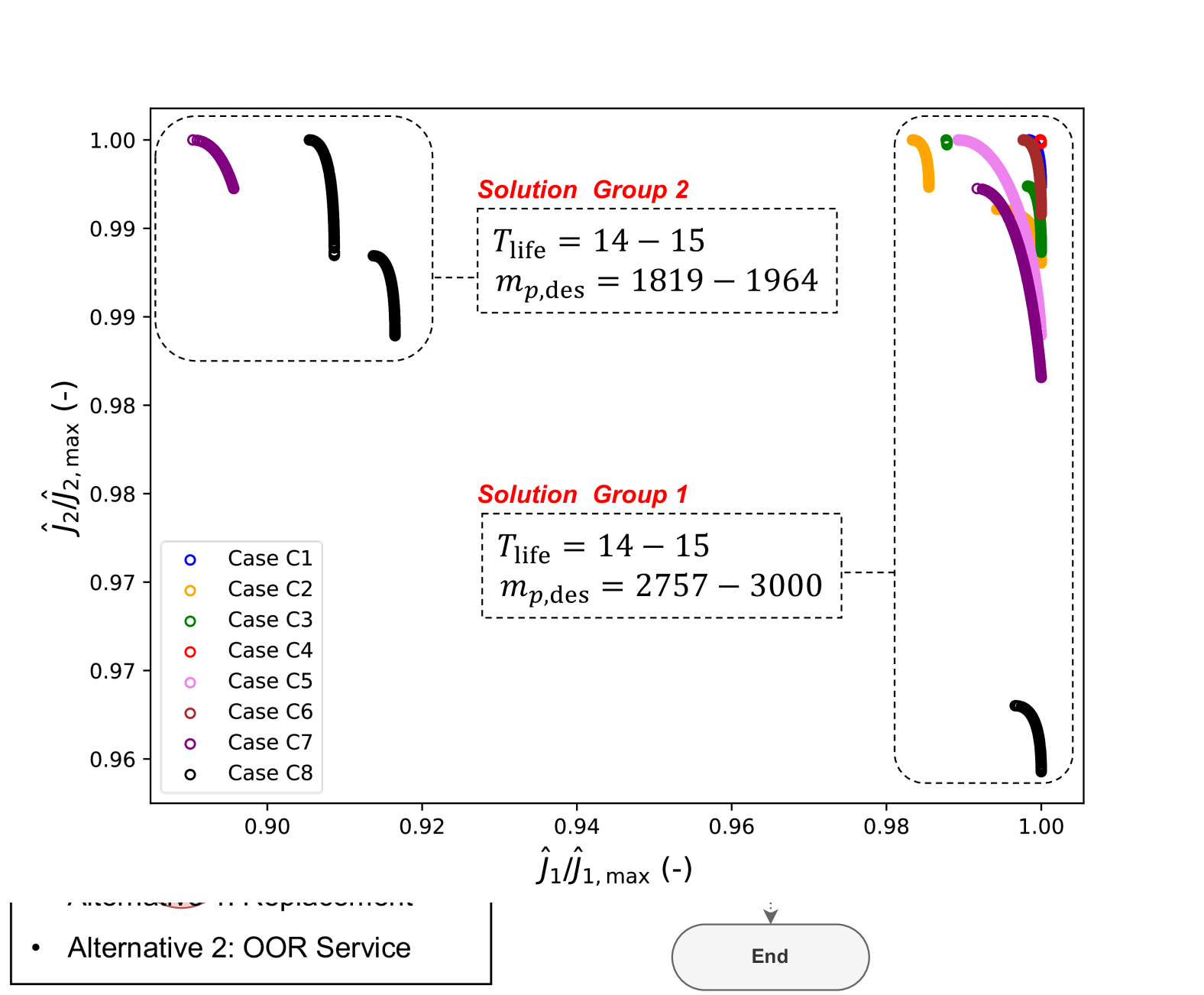
Figure 1: Flow diagram of the satellite lifecycle simulation

The assumptions made for the simulation are as follows:

1. Cost Incurrence: Cost is incurred at the time of the corresponding event. For example, a new satellite launch incurs the replacement cost, implying we focus on the launch event rather than the satellite manufacturing and launch contracting process.

2. Revenue Generation: Revenue occurs at time step $\left(t+1\right)$ if the satellite is operational at time step $t$ and time step $\left(t+1\right)$ without failure.

3. Independence of Uncertainties: Different types of uncertainties, such as market and technological advancement, are assumed to be independent.

4. Replacement Failure: This failure type includes catastrophic launch failure and the equipping of insufficient propellant for initial orbital transfer. No rescue strategy for satellites failing to reach the intended mission orbit is assumed.

5. Insurance Coverage: In the event of failures during replacement or OOR service, associated costs are assumed to be covered by insurance.

6. Technological Update: Every newly launched satellite is equipped with the latest technologies available at the time.

7. Exclusion of Project Abandonment: The option to abandon the project is not considered.

The simulation progresses by transitioning from one event to another. The event includes the Start and the End of the simulation, Decision, Action, and Failure. Figure 1 depicts the flow diagram of the simulation. As the simulation advances, these events occur in a sequential manner, incurring associated cash flows. The outcome of the simulation is the NPV ($V$), calculated as the discounted sum of these cash flows:

$$V=\sum_{t=1}^{t_{\text{sim}}}CF_{t}e^{-r_{f}t\Delta T},$$ (12)

where $CF_{t}$ is the cash flow at time step $t$, $r_{f}$ is the risk free rate, $\Delta T$ is the time step size in years, and $t_{\text{sim}}$ is the total number of simulation time steps. Given that the NPV results from stochastic events, its value varies with each execution, even under identical parameter settings. The rest of this section provides a detailed breakdown of the components constituting the simulation.

3.2.1 Start & End

The simulation initiates with the launch of a new satellite. It progresses until the simulation time ($t$) reaches $t_{\text{sim}}$, set as the endpoint. The mechanism for monitoring the attainment of this endpoint, $t_{\text{sim}}$, is integrated within Normal Operation.

3.2.2 Normal Operation

The Normal Operation represents the period when the satellite functions as originally intended. The simulation does not take action during the Normal Operation period. Instead of being a distinct event, Normal Operation is a transitional phase between two consecutive events, maintaining a normally operational state. During this phase, the simulation checks whether it has reached its endpoint. If the end is reached, the simulation concludes. Otherwise, it continues to the next event.

For each time step, the satellite consumes propellant for station-keeping maneuvers. The cumulative $\Delta V$ required for station-keeping maneuver over $t_{\text{prog}}$ time steps ($\Delta V_{\text{stk}}$) increases proportionally with the number of these time steps:

$$\Delta V_{\text{stk}}\left(t_{\text{prog}}\right)=t_{\text{prog}}\Delta v_{\text{stk}},\quad\Delta v_{\text{stk}}=\Delta V_{\text{stk,yr}}\Delta T$$ (13)

Here, $\Delta V_{\text{stk},\text{yr}}$ is $\Delta V$ required for station-keeping maneuver annually. The propellant consumption for this maneuver is determined by the rocket equation, which represents the relation between the required $\Delta V$, the performance of the propulsion subsystem, and the propellant consumption:

$$m_{p}=m_{0}\left(1-\exp\left(-\frac{\Delta V}{g_{0}I_{\text{sp}}}\right)\right)$$ (14)

Here, $\Delta V$ is the $\Delta V$ value required for a specific maneuver, $m_{p}$ is the corresponding propellant consumption, and $m_{0}$ is the initial gross mass of the satellite.

As a result of the operation, the revenue and cost associated with satellite operation are incurred. The associated revenue is determined dynamically. In the simulation, the dynamic environmental factors affecting the revenue generated by satellite operations are technology obsolescence and market volatility. These factors significantly influence the decision-making process regarding the design lifetime of a system [8]. The revenue generated from satellite operations is calculated by multiplying these factors with the baseline revenue:

$$R\left(T\right)=R_{0}\phi_{\text{mar}}\left(T\right)\phi_{\text{obs}}\left(T;T^{\prime}\right),$$ (15)

where $T^{\prime}$ denotes the reference time for the level of the applied technology. The market factor ($\phi_{\text{mar}}$) follows a geometric Brownian motion [8, 30]. The discrete version of the stochastic differential equation is as follows:

$$\Delta\phi_{\text{mar}}=\mu_{\text{mar}}\Delta T+\sigma_{\text{mar}}\epsilon\sqrt{\Delta T}.$$ (16)

Also, the technology obsolescence factor ($\phi_{\text{obs}}$) is defined as follows [8]:

$$\phi_{\text{obs}}\left(T;T^{\prime}\right)=\exp\left(-\left(\frac{T-T^{\prime}}{T_{\text{obs}}}\right)^{2}\right).$$ (17)

During Normal Operation, satellites are subject to in-orbit failures caused by component malfunctions. One can model the time to a certain type of in-orbit failure using a probability distribution (e.g., Weibull distribution). A simple yet effective model to describe the overall failure behavior of a satellite is the 2-Weibull distribution model. This model can capture the dynamic characteristics of in-orbit failure types, including infant mortality and wear-out failures [31]. The reliability function ($Rel$) following the 2-Weibull distribution is expressed as follows:

$$Rel\left(T\right)=\alpha\exp\left(-\left(\frac{T}{\theta_{1}}\frac{T_{\text{ref}}}{T_{\text{life}}}\right)^{\beta_{1}}\right)+\left(1-\alpha\right)\exp\left(-\left(\frac{T}{\theta_{2}}\frac{T_{\text{ref}}}{T_{\text{life}}}\right)^{\beta_{2}}\right),\quad T\in\mathbb{R}_{+},$$ (18)

where $T_{\text{ref}}$ is the reference design lifetime, $T_{\text{life}}$ is the design lifetime, and $\alpha$, $\beta_{1}$, $\beta_{2}$, $\theta_{1}$, and $\theta_{2}$ are parameters of the 2-Weibull distribution. In this equation, the first term containing the parameter $\beta_{1}(<1)$ represents the infant mortality phase, and the second term, characterized by the parameter $\beta_{2}(>1)$, reflects the wear-out phase.

3.2.3 Decision

Decision is a critical event that models the operational flexibility of the satellite operator. This event has two types, each with its specific timing and set of available alternatives (Fig. 2). At each Decision event, the most suitable alternative is selected from the available alternatives. The action chosen yields varying results, depending on the interaction between the altered state of the satellite and the external environment involving uncertainty.

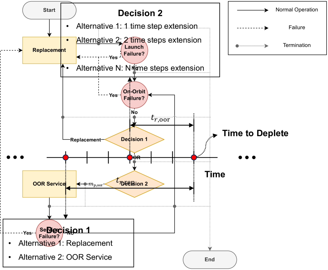
Figure 2: Decision timings and alternatives

The best alternative is chosen based on the predefined utility function for each alternative. The detailed formulations of the utility functions are provided in Appendix A.2 and A.3. Assumptions regarding the satellite operator’s information and preferences are established to define these utility functions:

1. The operator is fully informed about the dynamic and stochastic models of the system, including reliability, launch and service failures, market volatility, and technology obsolescence.

2. The operator employs a greedy decision-making approach, prioritizing the financial gains before making the next decision.

Decision 1 is initiated $t_{r,\text{rep}}$ time steps before the projected propellant depletion. At that point, the operator decides whether to replace or replenish the satellite—corresponding to Replacement and OOR Service actions. If the Replacement has a higher utility than OOR Service, then the Replenishment is scheduled after $t_{r,\text{rep}}$ time steps, which is the time required to manufacture and launch for replacement.

Decision 2 is triggered after OOR is selected in Decision 1. It occurs $t_{r,\text{oor}}$ ($<t_{r,\text{rep}}$) time steps before the projected depletion. This event determines the quantity of propellant for refueling. The life-extension period provided by OOR Service is determined as the period with the highest utility, similar to Decision 1. When a specific life-extension duration is selected, OOR Service with the corresponding propellant amount ($m_{p,\text{oor}}$) is planned after $t_{r,\text{oor}}$ time steps.

3.2.4 Action

Action marks an event where a specific action, Replacement, or OOR Service is executed. This action is determined by the decision made in the previous Decision event or is initiated by Failure. The Action event plays a role as a bridge between decision-making and operational execution, leading to a change in the state of the satellite.

Each action is associated with distinct failures. In the event of a failure during the replacement or OOR, the simulation proceeds to Failure. If no failure occurs, the associated costs of the satellite replacement or OOR service are incurred. Subsequently, the system’s state is altered, leading the simulation to progress to the next event.

In Replacement, the satellite currently in orbit is substituted with a new one. Replacement is successful if the launch and the orbital transfer are performed successfully. Launch is failed by a probability of $p_{f,\text{lau}}$. In addition, the orbital transfer is successful if the initially loaded propellant is enough to accomplish the maneuvers. The following equation represents the probability of replacement failure ($p_{f,\text{rep}}$), considering launch failure rate ($p_{f,\text{lau}}$) and orbital transfer successes:

$$p_{f,\text{rep}}=1-\left(1-p_{f,\text{lau}}\right)P\left[m_{p,\text{ot}}\leq m_{p,\text{des}}\right],$$ (19)

where $P\left[m_{p,\text{ot}}\leq m_{p,\text{des}}\right]$ denotes the probability that the design propellant mass, $m_{p,\text{des}}$, is at least as large as the required propellant for the orbital transfer, $m_{p,\text{ot}}$ (i.e., the likelihood of a successful orbital transfer). To obtain this value, a stochastic model of $m_{p,\text{ot}}$ is required.

Launch service providers give the accuracy of the orbit injection to their customers. For instance, the Ariane 5 User’s Manual [32] specifies the injection accuracy data of geostationary transfer orbit (GTO) mission as detailed in Table 2.

Table 2: GTO injection accuracy of Ariane 5 [32]

Description	Notation	Standard Deviation
Semi-major axis deviation (km)	$a$	40
Eccentricity deviation	$e$	4.5E-4
Inclination deviation (deg)	$i$	0.02
Argument of perigee deviation (deg)	$\omega$	0.2
Right ascension of the ascending node deviation (deg)	$\Omega$	0.2

Correcting such errors requires additional $\Delta V$ for the orbital transfer phase. We model this as a half-normal distribution:

$$\Delta V_{\text{ot}}=\Delta V_{\text{ot},\text{ideal}}+\Delta V_{\text{err}},\quad\Delta V_{\text{err}}\sim\mathcal{H}\left(\sigma_{\text{oi}}\right),$$ (20)

where $\Delta V_{\text{ot}}$ and $\Delta V_{\text{ot},\text{ideal}}$ represent the actual and ideal $\Delta V$ required for orbital transfer from the initial orbit to the target orbit, respectively, and $\Delta V_{\text{err}}$ is the additional $\Delta V$ needed for injection error correction. Here, $\mathcal{H}\left(\sigma_{\text{oi}}\right)$ denotes a half-normal distribution derived by taking the absolute value of a normal distribution with mean $0$ and standard deviation $\sigma_{\text{oi}}$.

Combining this with Eq. (14), the propellant mass and $\Delta V$ relationship, as described by the rocket equation, explains the second term in Eq. (19):

$$P\left[m_{p,\text{ot}}\leq m_{p,\text{des}}\right]=P\left[\Delta V_{\text{ot}}\leq g_{0}I_{\text{sp}}\ln\left(m_{\text{wet}}/m_{\text{dry}}\right)\right]=2\left(\Phi\left(\min\left(\frac{g_{0}I_{\text{sp}}\ln\left(m_{\text{wet}}/m_{\text{dry}}\right)-\Delta V_{\text{ot}}}{\sigma_{\text{oi}}},0\right)\right)-0.5\right).$$ (21)

In the OOR Serivce, the satellite currently in orbit is refueled with the amount of propellant determined in the previous Decision 2. The OOR Service is subject to the risk of service failure, which occurs if any step in the series of maneuvers—including rendezvous, proximity operation, docking, undocking (RPODU)—or robotic manipulation for the servicing activity fails. These failures can lead to various levels of malfunction, ranging from minor functional degradation and delayed service to the total loss of the client satellite. In this research, we only consider catastrophic failures resulting in a total loss of the satellite, characterized by a probability of $p_{f,\text{serv}}$.

3.2.5 Failure

The simulation includes three distinct types of failures to represent the realistic risks in satellite operations: in-orbit failure during the Normal Operation, replacement failure at the Replacement, and service failure during the OOR Service, as previously introduced. Upon any of these failures, the Replacement is planned $t_{r,\text{rep}}$ time steps after the failure occurs.

4 Satellite System Architecting Framework

The outputs from the lifecycle simulation developed in the previous section serve as substitutes for the objective functions of $\mathbf{P}_{\text{O}}$. Since the simulation unfolds as a series of stochastic events and produces NPV as a result, the objective functions of $\mathbf{P}_{\text{O}}$, which consist of statistical measures of NPV, can only be estimated by repeatedly running the simulation. This sampling-based estimation, commonly known as the Monte Carlo method, presents two main difficulties in optimization: 1) the same set of design variables under the same scenario may yield different estimation results each time; and 2) conducting repetitive simulations is computationally expensive, especially given that optimization processes typically involve iterative computations.

Figure 3: Proposed satellite system architecting framework

In this research, we propose a simple surrogate model-based optimization framework to address these difficulties. Figure 3 describes the overall procedure. The rest of this section details the processes of this framework: Scenario Set-up, Surrogate Model Formulation, and Solution & Analysis.

4.1 Scenario Set-up

The simulation parameters reflecting the scenario of interest are set. Following this, the design space is defined. It should encompass a meaningful range of values for the design variables while being appropriately constrained to enhance the computational efficiency of the optimization. For example, the meaningful range of $T_{\text{life}}$ can be defined by the effective range of MER and CER, here, from 3 to 15 years. Through this process, the target scenario is set up.

4.2 Surrogate Model Formulation

After the scenario is set, the processes for generating surrogates that substitute for the objective functions are initiated. First, a surrogate model is selected. The alternatives range from simple linear regression with polynomials to more flexible non-parametric models, such as Gaussian process regression or neural networks. Multiple models can be selected and processed simultaneously, and the best one can be adopted after being assessed. For example, Gaussian processes with different kernels can be selected as candidates [33].

Following the model selection, a set of experiment design variables, $A\subset X$, is defined. This set should consist of adequate samples of the design space to ensure that the trained models can effectively mimic the simulation results. At the same time, the number of experimental points, $|A|$, should be regulated to balance the computational burden. Given the simulation’s complexity and non-linear nature, an appropriate selection strategy should be considered [34].

For each element in this set, $N$ Monte Carlo simulations are executed, and the sample mean, $\overline{V}_{i}$, and sample standard deviation, $S_{i}$, of NPV are used as unbiased estimations of the mean and standard deviation of the NPV:

$$\overline{V}_{i}=\frac{1}{N}\sum_{j=1}^{N}V_{ij},\quad 1\leq i\leq\left|A\right|,$$ (22)

$$S_{i}=\sqrt{\frac{1}{N-1}\sum_{j=1}^{N}\left(V_{ij}-\overline{V}_{i}\right)^{2}},\quad 1\leq i\leq\left|A\right|,$$ (23)

where $i$ is the index for each experimental point in $A$, $j$ is the index for each experiment result among $N$ simulations, $\overline{V}_{i}$ is the sample mean of the $i$th experimental point, $S_{i}$ is the sample standard deviation of the $i$th experimental point, and $V_{ij}$ is the $j$th result of the $i$th experimental point. These estimations converge to corresponding values as $N$ increases, though this also escalates the computational burden, necessitating a careful determination of $N$ [35].

The results of these experiments aggregate to form datasets $\mathcal{D}_{1}$ and $\mathcal{D}_{2}$, comprising input-output pairs used for training the surrogate models for the objective functions:

$$\mathcal{D}_{1}=\bigl{\{}\bigl{(}\mathbf{x}_{i},\overline{V}_{i}\bigr{)}\bigr{\}}_{1\leq i\leq\left|A\right|},\quad\mathcal{D}_{2}=\bigl{\{}\bigl{(}\mathbf{x}_{i},\overline{V}_{i}/S_{i}\bigr{)}\bigr{\}}_{1\leq i\leq\left|A\right|}.$$ (24)

The performance of the trained model is assessed using the test sets. These sets are constructed similarly to the training sets but with design variables randomly sampled from the design space. The value of a performance metric, such as $R^{2}$, is calculated to evaluate the model’s efficacy. If the performance is unsatisfactory, the process cycles back to either model selection or experiment design, repeating the procedure until satisfactory performance levels are attained.

4.3 Solution & Analysis

If the surrogates for the objective functions demonstrate satisfactory performance, they are set to substitute for the objective functions of the original problem ($\mathbf{P}_{\text{O}}$):

($\mathbf{P}_{\text{SO}}$) Surrogate-Assisted Optimization of Satellite System Architecture

$$\underset{\mathbf{x}}{\text{maximize}}\ \mathbf{\hat{J}}\left(\mathbf{x}\right)=\left[\hat{J}_{1},\hat{J}_{2}\right]^{\top}$$ (25)

subject to

$$\mathbf{x}\in X.$$ (26)

In this formulation, $X$ denotes the feasible set from the original problem. The surrogate functions, $\hat{J}_{1}$ and $\hat{J}_{2}$, represent the surrogates for $E_{V}$ and $E_{V}/\sigma_{V}$, respectively. Utilizing these surrogate objective functions overcomes the difficulties mentioned earlier. Firstly, they provide deterministic output; if the input value remains constant, the output value will also be consistent, thereby facilitating the optimization process. Secondly, the surrogate models yield the output through simple arithmetic processes rather than complex simulations, easing the repetitive assessment of each design choice and thus streamlining the optimization process.

With the problem formulation now altered to suit a general optimization process, the selection of the optimization algorithm becomes relatively flexible. Metaheuristics such as NSGA-II [36] can be simple and effective to obtain the solutions.

After identifying efficient solutions, they undergo a thorough analysis. Building on the insights obtained from the analysis, a new scenario with different parameters can be established for further analysis. We showcase the detailed process and effectiveness of the framework in the next section.

5 Case Study: GEO Communication Satellite Architecting Considering OOR

This section discusses the systems architecting of GEO communication satellites considering OOR. Historically, these satellites have been pivotal in generating revenue by offering communication services to terrestrial customers. The focus of the GEO satellite design has been on improving its durability and longevity, aiming to develop a more reliable satellite capable of carrying a larger payload. Consequently, the launch weight of GEO communication satellites has escalated, now exceeding six metric tons [37].

The substantial costs and potential revenues associated with the lifecycle of GEO communication satellites have positioned them as primary targets for various OOS. The feasibility and practicality of the services have been demonstrated by life-extension missions, notably those conducted by the MEV-1/2 for Intelsat-901 and Intelsat 10-02 [38]. These missions, carried out by the MEV-1 and MEV-2, are prominent examples of the practical application and market interest in such services.

This case study diagnoses the current targeted service performance and analyzes critical service parameters influencing GEO communication satellite systems architecture. The case study is structured into three distinct scenarios in line with these objectives. The baseline scenario (Case A) aligns service parameters with those of current commercial benchmarks. The other two scenarios (Case B and Case C) investigate the impact of varying service parameters on the optimal architecture of the satellite system.

5.1 Case A: Baseline Scenario

Case A showcases the details of the solution procedure explained in Section IV and evaluates the current target service performance from the perspective of satellite system architecture. The process details are presented sequentially, and parameters are carefully selected to fulfill these objectives.

5.1.1 Scenario Set-up

Table 3 provides the system/environment parameters used in Case A. All cases (Cases A, B, and C) assume that the satellite uses a chemical propulsion system, which aligns with the refueling service proposed by Orbit Fab [39]. Another assumption is that the satellite is initially launched into a GTO and then maneuvers to a GEO using its onboard propulsion system. The perigee and apogee altitudes of the GTO are set at 200 km and 36,000 km, respectively. The simulation time is set to 30 years, with a time step of approximately two weeks to maintain adequate time resolution.

Table 3: Values of parameters for the baseline case simulation

Parameter	Notation	Value	Unit
Simulation time	$T_{\text{sim}}$	30	yr
Time step	$\Delta T$	1/24	yr
Reference design lifetime	$T_{\text{ref}}$	3	yr
$\Delta V$ required for orbital transfer from the ideal initial orbit to the target orbit	$\Delta V_{\text{ot}}$	1477	m/s
Parameter of $\Delta V$ distribution for correcting the orbit injection error	$\sigma_{\text{oi}}$	25	m/s
Reference mass	$m_{\text{ref}}$	1100	kg
Structural mass ratio	$r_{\text{str}}$	0.21	-
ADCS mass ratio	$r_{\text{adcs}}$	0.06	-
Mass growth rate of a satellite to the design lifetime	$\kappa$	0.03	-
Coefficients for propulsion subsystem mass	$a_{\text{prop}}$	1.336	kg1/3
	$b_{\text{prop}}$	0.455	kg
Specific impulse of the propulsion subsystem	$I_{\text{sp}}$	230	sec
Parameters for reliability function	$\alpha$	0.9490	-
	$\beta_{1}$	0.4458	-
	$\beta_{2}$	4.6687	-
	$\theta_{1}$	39830.5	yr
	$\theta_{2}$	9.8	yr
Time to replacement	$T_{r,\text{rep}}$	3	yr
Launch failure rate	$p_{f,\text{lau}}$	0.03	-
Annual $\Delta V$ required for station-keeping	$\Delta V_{\text{stk},\text{yr}}$	50	m/s
Specific satellite acquisition cost	$c_{\text{sat}}$	0.12	$M/kg
Specific launch cost	$c_{\text{lau}}$	0.01	$M/kg
Operational cost ratio	$r_{\text{op}}$	0.1	-
Insurance cost ratio	$r_{\text{ins}}$	0.2	-
Servicing interface mass ratio	$r_{\text{serv}}$	0.01	-
Variable cost coefficient of OOR service	$c_{v,\text{oor}}$	0.2	$M/kg
Fix cost of OOR service	$c_{f,\text{oor}}$	5	$M
OOR service capacity	$M_{\text{oor}}$	100	kg
OOR service failure rate	$p_{f,\text{oor}}$	0.03	-
Initial operational revenue	$R_{0}$	70	$M/yr
Risk free rate	$r_{f}$	0.03	-
Market drift rate	$\mu_{\text{mar}}$	0.03	yr-1
Market volatility	$\sigma_{\text{mar}}$	0.1	yr-1
Parameter for technology obsolescence	$T_{\text{obs}}$	20	yr

The parameters for the MER—$r_{\text{str}}$, $r_{\text{adcs}}$, and $\kappa$—are taken from Saleh et al. [7]. Additionally, $a_{\text{prop}}$ and $b_{\text{prop}}$ are determined by fitting the model presented in Eq. (6) to the mass data of high Earth orbit satellites [40]. The reference mass ($m_{\text{ref}}$) is set to 1100 kg. With a design lifetime of $T_{\text{life}}=15$ years and a design propellant mass of $m_{p,\text{des}}=3000$ kg, the resulting dry mass is $m_{\text{dry}}=1661$ kg, which is within a reasonable range. The parameters for the reliability function—$\alpha$, $\beta_{1}$, $\beta_{2}$, $\theta_{1}$, and $\theta_{2}$—are adopted from Saleh and Castet [31], and the remaining parameters are set based on data from existing articles [8, 23, 40] to ensure they fall within a reasonable range.

The baseline service cost and capacity are derived from available data at the moment, including the Orbit Fab’s target service performance [5] and Showalter et al. [41]. Given the nascent stage of commercial OOR services, we have made several conservative estimates. These include a higher failure rate, in line with current launch failure statistics, exceeding the rate discussed in another study [23]. Additionally, the service interface mass ratio is set at 1%, which is higher than existing market projections for products such as docking plates and fuel valves [42, 39]. The estimated time for completing the OOR service is approximately one month, a conservative estimate considering the time required for RPODU maneuvers in GEO.

The design space $X$ is defined as Table 4. Here, we select the range of the design lifetime following the range studied in [7], which the MER and CER are based on. Also, the range of design propellant mass is selected that covers from the minimum to the maximum with the given performance of the propulsion subsystem and the mass parameters.

Table 4: Design space for case study

Design variable	Notation	Range	Unit
Design lifetime	$T_{\text{life}}$	$\left[3,15\right]$	yr
Design propellant mass	$m_{p,\text{des}}$	$\left[1000,3000\right]$	kg

5.1.2 Surrogate Problem Formulation

This study selects Gaussian processes with various kernels as surrogate model candidates. These kernels include the squared exponential (SE), Matérn 5/2, and Matérn 3/2 [33]. Each kernel corresponds to differentiability classes $C^{\infty}$, $C^{2}$, and $C^{1}$, respectively. The SE kernel is known for its smoothness, making it ideal for capturing continuous trends, whereas the Matérn kernels are selected for their ability to model less smooth phenomena.

We employ a full factorial design approach to sample experimental points for training these models. Specifically, the design lifetime is segmented into 1-year intervals, and the design propellant mass is segmented into 100 kg increments. This segmentation results in 13 distinct levels for the design lifetime and 21 levels for the design propellant mass, culminating in 273 variable combinations. These combinations form the set of experimental points, $A$.

For each experimental point, 1000 Monte Carlo simulations are executed. As a result, the datasets $\mathcal{D}_{1}$ and $\mathcal{D}_{2}$ are generated. These datasets train all the candidate models. As a result of the training process, the hyperparameters of each model are updated to maximize the marginal likelihood [33].

Table 5: Training result: Case A

Kernel	Objective Function	$R^{2}$
SE	$J_{1}$	0.930
	$J_{2}$	0.927
Matérn 5/2	$J_{1}$	0.933
	$J_{2}$	0.930
Matérn 3/2	$J_{1}$	0.935
	$J_{2}$	0.932

The test set assesses the trained models. The design variables for the test set are sampled uniformly at random within the design space. The performance of each model is provided in Table 5, as $R^{2}$. The result reveals that all kernel alternatives for each objective function achieve $R^{2}$ values exceeding 0.9 in the test phase. This result implies that the uniform design strategy and the segmentation resolution are appropriate for this situation. Among the kernel alternatives, Matérn 3/2 exhibits the highest score, the roughest kernel among the alternatives. Consequently, the Gaussian process with Matérn 3/2 is selected for the surrogate model to be used in the subsequent optimization process.

Figure 4 provides contour plots with heatmaps for the selected surrogate model corresponding to each objective function. It shows that $\hat{J}_{1}$ has a peak at the maximum design lifetime and propellant mass, whereas $\hat{J}_{2}$ exhibits two peaks—one at the maximum design lifetime and propellant mass and another at a reduced design lifetime and propellant mass.

Figure 4: Contour plot and heatmap of $\hat{J}_{1}$ (left) and $\hat{J}_{2}$ (right) with peaks (red dots)

5.1.3 Solution & Analysis

A set of efficient solutions is obtained using NSGA-II [36] as the optimization algorithm. Figure 5 depicts these solutions graphically within varying scales, where the x-axis and y-axis represent the first and second objectives, respectively. Here, all solutions converge on a 15-year design lifetime, while the propellant mass fluctuates within a limited range, from 2865 to 2961 kg. This range suggests sufficient propellant reserves for all solutions throughout the design lifetime.

This solution consistency reveals a common design strategy—prioritizing lifetime maximization while ensuring enough propellant throughout the design lifetime. Consequently, all solutions can be classified as a single architectural group, which aligns with contemporary satellite design and operational trends. This finding implies that modifying the satellite system architecture presents minimal potential benefit under the given service performance.

Figure 5: Pareto efficient solutions plots with different scales: Case A

5.2 Case B: Identifying Critical Service Parameters

Dual objectives drive Case B: first, evaluating the economic feasibility of adopting a new architecture by optimistic service performance; second, identifying key service parameters influencing the optimal solutions of the satellite system architecture. To achieve these objectives, Case B sets idealized service parameters in Table 6 for assessing their impact on architectural decisions.

Table 6: Ideal service parameters

Parameter	Notation	Value	Unit
Variable cost coefficient of OOR service	$c_{v,\text{oor}}$	0.02	$M/kg
Fix cost of OOR service	$c_{f,\text{oor}}$	0.5	$M
OOR service capacity	$M_{\text{oor}}$	2000	kg
OOR service failure rate	$p_{f,\text{oor}}$	0	-

Highlights of these ideal scenarios include a significant service cost reduction of one-tenth compared to the baseline, idealized service capacity treated as unlimited with 2000 kg, and eliminated service failures. Seven subcases with distinct service parameter combinations in Table 7 are defined to assess individual and combined parameter effects. The initial three subcases, B1–B3, isolate the impact of individual parameters by setting each to its ideal value while holding the others at their baseline. Subcases B4–B6 explore the synergy of different parameters by experimenting with the combined effects of paired parameters in their ideal settings. Finally, subcase B7 sets all parameters to their ideal values.

Table 7: Service parameters combinations of each subcase of Case B

Case	Cost	Capacity	Failure Rate
B1	Ideal	Baseline	Baseline
B2	Baseline	Ideal	Baseline
B3	Baseline	Baseline	Ideal
B4	Ideal	Ideal	Baseline
B5	Baseline	Ideal	Ideal
B6	Ideal	Baseline	Ideal
B7	Ideal	Ideal	Ideal

Figure 6: Pareto efficient solutions plots in the normalized objective space: Case B

We obtain the Pareto efficient solutions for each subcase in Case B using the same methodology as in Case A. Figure 6 plots the obtained solutions from all the cases in the normalized objective space. Subcases B1, B4, B6, and B7 are notable for presenting two distinct solution groups. In contrast, the other subcases feature a singular solution group (Solution Group 1), mirroring the solutions observed in Case A, typically characterized by design lifetimes of 14 or 15 years and sufficient propellant mass for the entire operational period.

However, an alternative solution group (Solution Group 2) emerges in Cases B1, B4, B6, and B7, diverging significantly from the conventional designs. This group is characterized by similar design lifetimes—13 to 14 years—but with a significantly reduced design propellant mass, relying on OOR services for approximately 50% or more of the station-keeping maneuvers during their operation. Despite a lower expected return, this alternative approach offers a higher return per risk and is viable primarily in scenarios with optimistic service cost parameters.

These findings imply that lower service costs are essential for motivating the architectural design change of GEO communication satellites in the given scenario.

5.3 Case C: Specifying cost threshold

The findings from Case B establish service cost as a critical parameter in the economic viability of alternative satellite system architectures. Given these insights, it is essential for satellite operators to proactively monitor and adapt to the evolving landscape of service costs, strategically aligning their decisions with cost-efficient solutions. This understanding forms the basis of Case C, which aims to pinpoint the specific cost threshold where alternative architectures gain economic efficiency.

Case C consists of 8 subcases, each with the baseline parameters but with varying service costs, scaled from 0.9 to 0.2 of the baseline value. Notably, we exclude a subcase with a service cost of 0.1 of the baseline, which is already examined under Case B as Case B1. The service cost parameters for each subcase in Case C are delineated in Table 8.

Table 8: Service cost parameters of each subcase of Case C

	Cost Parameters
Case	$c_{v,\text{oor}}$	$c_{f,\text{oor}}$
C1	0.18	4.5
C2	0.16	4.0
C3	0.14	3.5
C4	0.12	3.0
C5	0.10	2.5
C6	0.08	2.0
C7	0.06	1.5
C8	0.04	1.0

Figure 7: Pareto efficient solutions plots in the normalized objective space: Case C

The Pareto efficient solutions for each subcase within Case C are derived using the same process as in Cases A and B. Figure 7 represents these outcomes in the normalized objective space. Notably, in Case C7, where the service cost is 0.3 of the baseline case, an alternative group of efficient architectural solutions emerges. This observation suggests that a cost threshold for alternative architectural viability lies between 0.3 and 0.4 of the baseline service cost. This result provides insight into the economic feasibility of varying satellite system architectures under decreased service costs.

6 Conclusions

This paper introduces a satellite system architecting (high-level design) problem with explicit consideration of commercial OOR service. The design problem, formulated as a bi-objective optimization, can answer the questions of “How durable should the satellite be?” and “How much propellant should be loaded at launch?”. This optimization problem adopted the design lifetime and propellant as design variables, with return and risk metrics analogous to those in Portfolio Selection theory as dual objective functions. A surrogate model-based solution framework for this problem was developed based on a satellite lifecycle simulation. The simulation incorporated uncertainties and operational flexibilities, and integrated satellite sizing and cost models—revised from conventional MER and CER—to reflect the architectural implications of OOR. Furthermore, an independent servicing cost model was adopted, independent of a specific servicing infrastructure. The whole aggregate of the proposed formulation and solution methodology overcame the limitations of traditional approaches for evaluating satellite system architectures with OOR.

We conducted a case study on GEO communication satellites to demonstrate the effectiveness of our framework. This study involved analyzing potential future scenarios. From this case study, we found that, in the given scenario, the current target service performance of GEO communication satellites does not motivate architectural changes based solely on cost-effectiveness. Additionally, we found that a reduction in service costs—to approximately one-third of the current target service cost—is critical for the emergence of alternative architectural design solutions. This cost reduction requires not only the technological advancement of the OOR service provider but also the active participation of all market players, including OOR customers, who should equip their satellites with service-friendly designs, as well as support from governments, as noted in another study [6].

This study, primarily focusing on satellite system architecture selection within the context of OOR commercialization, holds the potential for expansion into a broader framework for various classes of OOS (e.g., maintenance and upgrade). A vital aspect of this expansion is the exploration of replaceable or repairable subsystems (e.g., structural and electrical components) that align with evolving OOS technologies. This exploration necessitates a detailed analysis of each subsystem’s reliability-sizing relations, as well as an assessment of performance degradation over time. It also requires reviewing design and operational strategies, along with additional design considerations, such as modular design, that facilitate servicing activities. The analysis should evaluate the impact on the satellite system’s lifecycle costs and revenue dynamics. Conducting this analysis is crucial for understanding the implications of integrating OOS into space systems. This in-depth insight will enable a more accurate evaluation of OOS, leading to better-informed decision-making and, ultimately, more profitable and sustainable space utilization in the long run.

Appendix

6.1 Utility Function of Each Alternative

6.1.1 Preliminaries

The DCF method is one of the most well-known appraisal approaches for engineering projects, classified under the income approach of business valuation [28]. This method involves a detailed estimation of the project’s expected net cash flows—referred to as Free Cash Flow (FCF)—throughout its lifecycle. Given that FCF is projected over a specific time horizon, it is essential to account for the time value of money, as the value of identical cash differs between the present and the future. To address this, each projected cash flow is discounted to its present value. Moreover, due to the inherent uncertainty in FCF projections, the DCF method also incorporates risk considerations alongside the time value of money. Consequently, FCF is converted to its present value using a discount rate that captures both the time value of money and the associated risks, thereby yielding an estimate of the project’s present economic value. Since we model associated risks in the events of the simulation, we use risk free rate, $r_{f}$, that not considers the risk, and the NPV is represented as

$$P=\sum_{T\in\mathcal{T}}CF_{t}e^{-rT},$$ (27)

where $P$ is the present value of the project, $CF_{t}$ is the free cash flow at time $T$, $r$ is the continuously compounded discount rate, and $\mathcal{T}$ is the set of times at which a cash flow occurs.

While NPV provides a single value that facilitates straightforward, quantitative decision-making, it may not offer a fair comparison between projects with differing durations. In such scenarios, an Equivalent Annuity (EA) approach can be employed, where a uniform cash flow amount of $A$ is determined to equate its NPV to that of the project’s varying cash flows. This metric $A$ allows for a more equitable comparison across projects of varying lifespans by accounting for each project’s duration. The mathematical relationship between NPV and EA is given by

$$A/P\left(r,N\right)=\frac{e^{rN}\left(e^{r}-1\right)}{e^{rN}-1},$$ (28)

where $N$ is the interest rate period.

Let $P[t_{\text{oof}}=t_{1};t_{0}]$ denote the probability of an in-orbit failure occurring at time step $t_{1}$ given that the satellite began operations at time step $t_{0}$. Recognizing that the time horizon is discretized while failures can occur at any continuous point, a failure occurring between time steps $t$ and $\left(t+1\right)$ is regarded as happening at time step $t$. The probability is thus defined via the reliability function as:

$$P[t_{\text{oof}}=t_{1};t_{0}]=Rel\left(T_{1}-T_{0}\right)-Rel\left(T_{1}-T_{0}+\Delta T\right),$$ (29)

where $T_{1}-T_{0}$ represents the elapsed time until failure. Consequently, the cumulative probabilities for failure occurring on or after, and on or before a certain time step, are defined as:

$$P[t_{\text{oof}}\geq t_{1};t_{0}]=\sum_{t=t_{1}}^{t_{\text{life}}}P[t_{\text{oof}}=t_{1};t_{0}]$$ (30)

$$P[t_{\text{oof}}\leq t_{1};t_{0}]=\sum_{t=0}^{t_{1}}P[t_{\text{oof}}=t_{1};t_{0}]$$ (31)

Let $R\left(t_{0}\right)$ denote the revenue provided by an operational satellite at time step $t_{0}$. The expected revenue at time step $t$ is represented as

$$\mathbb{E}\left[R\left(t\right);t_{0}\right]=R\left(t_{0}\right)\mathbb{E}\left[\phi_{\text{mar}}\left(T-T_{0}\right)\right]\phi_{\text{obs}}\left(T;T_{\text{op}}\right),$$ (32)

where $T_{\text{op}}$ denotes the time at which the satellite of interest begins operating.

The expected profits the operational satellite generates from Decision 1 until the next action is denoted by $EP_{1}$. Its mathematical expression is given by

$$EP_{1}\left(t\right)=\sum_{t_{1}=1}^{t_{r,\text{rep}}}\left(\left(1-r_{\text{op}}\right)\mathbb{E}\left[R\left(t+t_{1}\right);t\right]\frac{P\left[t_{\text{oof}}>t+t_{1};t_{\text{op}}\right]}{P\left[t_{\text{oof}}>t;t_{\text{op}}\right]}e^{-rT_{1}}\right),$$ (33)

where $\left(1-r_{\text{op}}\right)\mathbb{E}\left[R\left(t+t_{1}\right);t\right]$ denotes the expected cash flow at time step $t+t_{1}$, conditional on the operational satellite not having failed; $\frac{P\left[t_{\text{oof}}>t+t_{1};t_{\text{op}}\right]}{P\left[t_{\text{oof}}>t;t_{\text{op}}\right]}$ represents the conditional probability that the satellite remains operational at time step $t+t_{1}$ given that it is operational at time step $t$; is the continuously compounded discount factor, $e^{-rT_{1}}$ accounting for the time value of money.

Similarly, the expected profits the operational satellite generates from Decision 2 until the next action is denoted by $EP_{2}$:

$$EP_{2}\left(t\right)=\sum_{t_{1}=1}^{t_{r,\text{oor}}}\left(\left(1-r_{\text{op}}\right)\mathbb{E}\left[R\left(t+t_{1}\right);t\right]\frac{P\left[t_{\text{oof}}>t+t_{1};t_{\text{op}}\right]}{P\left[t_{\text{oof}}>t;t_{\text{op}}\right]}e^{-rT_{1}}\right).$$ (34)

6.1.2 Decision 1

In Decision 1, two alternatives are considered: replacement and OOR. The utility function for each alternative is defined according to the assumptions in Section 3. We define the utility function of the Replacement ($U_{\text{rep}}$) as the expected EA by the replacement. This utility function is defined as the sum of three distinct components, reflecting various possible outcomes of the replacement:

$$U_{\text{rep}}\left(t\right)=U_{\text{rep,1}}\left(t\right)+U_{\text{rep,2}}\left(t\right)+U_{\text{rep,3}}\left(t\right),$$ (35)

where $U_{\text{rep},1}$ represents the EA of the scenario where the replacement fails; $U_{\text{rep},2}$ represents the EA of the situation where the replacement is successful, but the replaced satellite either depletes its propellant or experiences an in-orbit failure before completing its designed operational lifetime; $U_{\text{rep},3}$ represents the EA of the case where the replacement is successful and the replaced satellite operates for its entire design lifetime. The mathematical representation of each term is as follows:

$$U_{\text{rep,1}}\left(t\right)=p_{f,\text{rep}}A/P\left(r,t_{r,\text{rep}}\right)EP_{1}\left(t\right),$$ (36)

$$U_{\text{rep,2}}\left(t\right)=\left(1-p_{f,\text{rep}}\right) \sum_{t_{1}=t_{r,\text{rep}}+1}^{t_{r,\text{rep}}+t_{\text{life}}-1}\Biggl{(}A/P\left(r,t_{1}\right)\biggl{(}EP_{1}\left(t\right)-C_{\text{IOC}}$$

$$+P\left[t_{\text{oof}}=t+t_{1};t+t_{r,\text{rep}}\right]\sum_{t_{2}=t_{r,\text{rep}}+1}^{t_{1}}\left(\mathbb{E}\left[R\left(t_{2}\right);t\right]e^{-rT_{1}}\right)\biggr{)}\Biggr{)},$$ (37)

$$U_{\text{rep,3}}\left(t\right)=\left(1-p_{f,\text{rep}}\right)P[t_{\text{oof}} \geq t_{r,\text{rep}}+t_{\text{life}};t+t_{r,\text{rep}}]A/P\left(r,t_{r,\text{rep}}+t_{\text{life}}\right)$$

$$\cdot\left(EP_{1}\left(t\right)-C_{\text{IOC}}+\sum_{t_{1}=t_{r,\text{rep}}}^{t_{r,\text{rep}}+t_{\text{life}}}\left(\mathbb{E}\left[R\left(t_{1}\right);t\right]e^{-rT_{1}}\right)\right).$$ (38)

The utility function of the OOR Service is defined as the maximum of the functions $u_{\text{oor}}(k;t)$ with respect to $k$:

$$U_{\text{oor}}(t)=\max_{k\in K_{t}}u_{\text{oor}}\left(k;t\right),$$ (39)

where $k$ denotes the number of time steps by which refueling extends the satellite’s operational lifetime, $u_{\text{oor}}(k;t)$ is the EA achieved by extending the satellite’s operational lifetime by $k$ time steps, and $K_{t}$ is available values of $k$ at time step $t$.

The required mass of propellant for extending the operational lifetime by $k$ time steps is given by:

$$m_{p,\text{oor}}\left(k;t\right)=\left(m_{\text{dry}}+m_{p,\text{rem}}\left(t\right)\right)\exp\left(-\frac{\Delta v_{\text{stk}}t_{r,\text{rep}}}{g_{0}I_{\text{sp}}}\right)\left(1-\exp\left(-\frac{\Delta v_{\text{stk}}k}{g_{0}I_{\text{sp}}}\right)\right),$$ (40)

where $m_{p,\text{rem}}\left(t\right)$ is the remaining propellant mass at time step $t$. Here, the term $\left(m_{\text{dry}}+m_{p,\text{rem}}\left(t\right)\right)\exp\left(-\frac{\Delta v_{\text{stk}}t_{r,\text{rep}}}{g_{0}I_{\text{sp}}}\right)$ represents the sum of the satellite’s dry mass and the remaining propellant mass after the time step $t_{r,\text{rep}}$. Additionally, the OOR service cost with refueling amount of $m_{p,\text{oor}}\left(k\right)$ is represented as

$$C_{\text{oor}}\left(k;t\right)=c_{v,\text{oor}}m_{p,\text{oor}}\left(k;t\right)+c_{f,\text{oor}},$$ (41)

following Eq (10). Since $m_{p,\text{oor}}$ is bounded by the service capacity ($M_{\text{oor}}$), the set of available values for $k$ ($K_{t}$) is defined as follows:

$$K_{t}=\left\{k\in\mathbb{Z}_{++}:m_{p,\text{oor}}\left(k;t\right)\leq M_{\text{oor}}\right\}.$$ (42)

Lastly, $u_{\text{oor}}\left(k;t\right)$ is defined as

$$u_{\text{oor}}\left(k;t\right)=u_{\text{oor},1}\left(t\right)+u_{\text{oor},2}\left(k;t\right)+u_{\text{oor},3}\left(k;t\right),$$ (43)

where the three terms are defined similarly to those in $U_{\text{rep}}$. Specifically, $u_{\text{oor},1}$ represents the EA of the scenario where the OOR service fails; $u_{\text{oor},2}$ represents the EA of the scenario where the OOR service is successful but the replenished satellite experiences an in-orbit failure before reaching its operational lifetime; $u_{\text{oor},3}$ represents the EA of the scenario where the OOR service is successful and the replenished satellite operates until depletion without any in-orbit failure. The mathematical representation of each term is as follows:

$$u_{\text{oor},1}\left(t\right)=p_{f,\text{oor}}A/P\left(r,t_{r,\text{rep}}\right)EP_{1}\left(t\right),$$ (44)

$$u_{\text{oor},2}\left(k;t\right)=\left(1-p_{f,\text{oor}}\right) \sum_{t_{1}=t_{r,\text{rep}}+1}^{t_{r,\text{rep}}+k-1}\Biggl{(}A/P\left(r,t_{1}\right)\biggl{(}EP_{1}\left(t\right)-C_{\text{oor}}\left(k;t\right)$$

$$+P\left[t_{\text{oof}}=t+t_{1};t_{\text{op}}\right]\sum_{t_{2}=t_{r,\text{rep}}+1}^{t_{1}}\mathbb{E}\left[R\left(t_{2}\right);t\right]\biggr{)}\Biggr{)},$$ (45)

$$u_{\text{rep,3}}\left(k;t\right)=\left(1-p_{f,\text{oor}}\right)P[t_{\text{oof}} \geq t_{r,\text{rep}}+t_{\text{life}};t_{\text{op}}]A/P\left(r,t_{r,\text{rep}}+t_{\text{life}}\right)$$

$$\left(EP_{1}\left(t\right)-C_{\text{oor}}\left(k;t\right)+\sum_{t_{1}=t_{r,\text{rep}}+1}^{t_{r,\text{rep}}+k}\left(\mathbb{E}\left[R\left(t_{1}\right);t\right]e^{-rT_{1}}\right)\right),$$ (46)

where $t_{\text{op}}$ is the time step where the currently operational satellite started its operation.

6.1.3 Decision 2

In Decision 2, a range of alternatives is considered, each corresponding to a different amount of propellant mass required for refueling. Similar to the approach in Decision 1, the utility function for each alternative is defined based on the assumptions in Section 3. In Decision 2, $u_{\text{oor}}\left(k;t\right)$ denotes the utility of extending the operation by OOR by $k$ time steps. The formulation parallels Eq (43), albeit with distinctions in the definitions of each term, as detailed below:

$$u_{\text{oor},1}\left(t\right)=p_{f,\text{oor}}A/P\left(r,t_{r,\text{oor}}\right)EP_{2}\left(t\right),$$ (47)

$$u_{\text{oor},2}\left(k;t\right)=\left(1-p_{f,\text{oor}}\right) \sum_{t_{1}=t_{r,\text{oor}}+1}^{t_{r,\text{oor}}+k-1}\Biggl{(}A/P\left(r,t_{1}\right)\biggl{(}EP_{2}\left(t\right)-C_{\text{oor}}\left(k;t\right)$$

$$+P\left[t_{\text{oof}}=t+t_{1};t_{\text{op}}\right]\sum_{t_{2}=t_{r,\text{oor}}+1}^{t_{1}}\mathbb{E}\left[R\left(t_{2}\right);t\right]\biggr{)}\Biggr{)}$$ (48)

$$u_{\text{oor},3}\left(k;t\right)=\left(1-p_{f,\text{oor}}\right)P[t_{\text{oof}} \geq t+t_{r,\text{oor}}+k;t_{\text{op}}]A/P\left(r,t_{r,\text{oor}}+k\right)$$

$$\left(EP_{2}\left(t\right)-C_{\text{oor}}\left(k;t\right)+\sum_{t_{1}=t_{r,\text{oor}}+1}^{t_{r,\text{oor}}+k}\mathbb{E}\left[R\left(t_{1}\right);t\right]\right)$$ (49)

References

-
[1]
Li, W.-J., Cheng, D.-Y., Liu, X.-G., Wang, Y.-B., Shi, W.-H., Tang, Z.-X., Gao, F., Zeng, F.-M., Chai, H.-Y, Luo, W.-B., Cong, Q., and Gao, Z.-L., “On-Orbit Service (OOS) of Spacecraft: A Review of Engineering Developments,” Progress in Aerospace Sciences, Vol. 108, Jul. 2019, pp. 32-120.
https://doi.org/10.1016/j.paerosci.2019.01.004 - [2] Arney, D., Sutherland, R., Mulvaney, J., Steinkoenig, D., Stockdale, C., and Farley, M., “On-Orbit Servicing, Assembly, and Manufacturing (OSAM) State of Play,” NASA TR 20210022660, 2021.
-
[3]
Davis, J. P., Mayberry, J. P., and Penn, J. P., “Game Changer: On-Orbit Servicing,” The Aerospace Corporation Center for Space Policy and Strategy, May 2019.
https://csps.aerospace.org/papers/game-changer-orbit-servicing -
[4]
Cavaciuti, A. J., Heying, J. H., and Davis, J., “Game Changer: In-Space Servicing, Assembly, and Manufacturing for the New Space Economy,” The Aerospace Corporation Center for Space Policy and Strategy, Jul. 2022.
https://csps.aerospace.org/papers/game-changer-space-servicing-assembly-and-manufacturing-new-space-economy - [5] Space News, “Orbit Fab Announces In-Space Hydrazine Refueling Service,” 2022, https://spacenews.com/orbit-fab-announces-in-space-hydrazine-refueling-service/[accessed 12 Jan. 2024].
-
[6]
Hastings, D. E., Putbrese, B. L., and La Tour, P. A., “When Will On-Orbit Servicing be Part of the Space Enterprise?,” Acta Astronautica, Vol. 127, Oct.-Nov. 2016, pp. 655-666.
https://doi.org/10.1016/j.actaastro.2016.07.007 -
[7]
Saleh, J. H., Hastings, D. E., and Newman, D. J., “Spacecraft Design Lifetime,” Journal of Spacecraft and Rockets, Vol. 39, No. 2, 2002, pp. 244-257.
https://doi.org/10.2514/2.3806 -
[8]
Saleh, J. H., Hastings, D. E., and Newman, D. J., “Weaving Time Into System Architecture: Satellite Cost per Operational Day and Optimal Design Lifetime,” Acta Astronautica, Vol. 54, No. 6, 2004, pp. 413-431.
https://doi.org/10.1016/S0094-5765(03)00161-9 -
[9]
Saleh, J. H., Torres-Padilla, J.-P., Hastings, D. E., and Newman, D. J., “To Reduce or to Extend a Spacecraft Design Lifetime?,” Journal of Spacecraft and Rockets, Vol. 43, No. 1, 2006, pp. 207-217.
https://doi.org/10.2514/1.10991 -
[10]
Saleh, J. H. “Flawed Metrics: Satellite Cost per Transponder and Cost per Day,” IEEE Transactions on Aerospace and Electronic Systems, Vol. 44, No. 1, 2008, pp. 147-156.
https://doi.org/10.1109/TAES.2008.4516995 -
[11]
Saleh, J. H., Lamassoure, E. S., Hastings, D. E., and Newman, D. J., “Space Systems Flexibility Provided by On-Orbit Servicing: Part 1,” Journal of Spacecraft and Rockets, Vol. 40, No. 2, 2003, pp. 551-560.
https://doi.org/10.2514/2.3944 -
[12]
Saleh, J. H., Lamassoure, E., and Hastings, D. E., “Space Systems Flexibility Provided by On-Orbit Servicing: Part 1,” Journal of Spacecraft and Rockets, Vol. 39, No. 4, 2002, pp. 551-560.
https://doi.org/10.2514/2.3844 -
[13]
Lamassoure, E., Saleh, J. H., and Hastings, D. E., “Space Systems Flexibility Provided by On-Orbit Servicing: Part 2,” Journal of Spacecraft and Rockets, Vol. 39, No. 4, 2002, pp. 561-570.
https://doi.org/10.2514/2.3845 -
[14]
Joppin, C., and Hastings, D. E., “On-Orbit Upgrade and Repair: The Hubble Space Telescope Example,” Journal of Spacecraft and Rockets, Vol. 43, No. 3, 2006, pp. 614-625.
https://doi.org/10.2514/1.15496 -
[15]
Long, A. M., Richards, M. G., and Hastings, D. E., “On-Orbit Servicing: A New Value Proposition for Satellite Design and Operation,” Journal of Spacecraft and Rockets, Vol. 44, No. 4, 2007, pp. 964-976.
https://doi.org/10.2514/1.27117 - [16] Lamassoure, E. S., “A Framework to Account for Flexibility in Modeling the Value of On-Orbit Servicing for Space Systems,” Master’s Thesis, Massachusetts Institute of Technology, Cambridge, MA, 2001.
- [17] Saleh, J. H., “Weaving Time Into System Architecture: New Perspectives on Flexibility, Spacecraft Design Lifetime, and On-Orbit Servicing,” Ph.D. Dissertation, Massachusetts Institute of Technology, Cambridge, MA, 2002.
- [18] Joppin, C., “On-Orbit Servicing for Satellite Upgrades,” Master’s Thesis, Massachusetts Institute of Technology, Cambridge, MA, 2004.
- [19] Long A. M., “Framework for Evaluating Customer Value and the Feasibility of Servicing Architectures for On-Orbit Satellite Servicing,” Master’s Thesis, Massachusetts Institute of Technology, Cambridge, MA, 2005.
- [20] Richards, M. G., “On-Orbit Serviceability of Space System Architectures,” Master’s Thesis, Massachusetts Institute of Technology, MA, 2006.
- [21] Mun, J., Real Options Analysis: Tools and Techniques for Valuing Strategic Investments and Decisions with Integrated Risk Management and Advanced Quantitative Decision Analytics, ed., ROV Press, Dublin, CA, 2016.
-
[22]
Yao, W., Chen, X., Huang, Y., and van Tooren, M., “On-Orbit Servicing System Assessment and Optimization Methods Based on Lifecycle Simulation Under Mixed Aleatory and Epistemic Uncertainties,” Acta Astronautica, Vol. 87, Jun.-July 2013, pp. 107-126.
https://doi.org/10.1016/j.actaastro.2013.02.005 -
[23]
Liu, Y., Zhao, Y., Tan, C., Liu, H., and Liu, Y., “Economic Value Analysis of On-Orbit Servicing for Geosynchronous Communication Satellites,” Acta Astronautica, Vol. 180, Mar. 2021, pp. 176–188.
https://doi.org/10.1016/j.actaastro.2020.11.040 - [24] Henry, C., “Intelsat-901 Satellite, With MEV-1 Servicer Attached, Resumes Service,” Space News, 2020, https://spacenews.com/intelsat-901-satellite-with-mev-1-servicer-attached-resumes-service/[accessed 12 Jan. 2024].
-
[25]
Markowitz, H., “Portfolio Selection,” The Journal of Finance, Vol. 7, No. 1, 1952, pp. 77–91.
https://doi.org/10.2307/2975974 -
[26]
Sharpe, W. F., “Mutual Fund Performance,” The Journal of Business, Vol. 39, No. 1, 1966, pp. 119–138.
https://www.jstor.org/stable/2351741 -
[27]
Marler, R. T., and Arora, J. S., “Survey of Multi-Objective Optimization Methods for Engineering,” Structural and Multidisciplinary Optimization, Vol. 26, Mar. 2004, pp. 396-395.
https://doi.org/10.1007/s00158-003-0368-6 - [28] Newman, D. G., Eschenbach, T. G., and Lavelle, J. P., Engineering Economic Analysis, ed., Oxford University Press, Oxford, United Kingdom, 2017.
-
[29]
Miles, J. A., and Ezzell, J. R., “The Weighted Average Cost of Capital, Perfect Capital Markets, and Project Life: A Clarification,” Journal of Financial and Quantitative Analysis, Vol. 15, No. 3, 1980, pp. 719-730.
https://doi.org/10.2307/2330405 - [30] Hull, J. C., Options, Future, and Other Derivaties, , Pearson Education, London, United Kingdom, 2022.
-
[31]
Saleh, J. H., and Castet, J.-F., Spacecraft Reliability and Multi-State Failures: A Statistical Approach, John Wiley & Sons, Hoboken, NJ, 2011.
https://doi.org/10.1002/9781119994077 -
[32]
Lagier, R., “Ariane 5 User’s Manual (Issue 5 Revision 2),” Arianespace Corp., Oct. 2016.
https://www.arianespace.com/wp-content/uploads/2011/07/Ariane5_Users-Manual_October2016.pdf [accessed 12 Jan. 2024]. -
[33]
Rasmussen, C. E., and Williams, C. K. I., Gaussian Process for Machine Learning, The MIT Press, Cambridge, MA, 2006.
https://doi.org/10.7551/mitpress/3206.001.0001 - [34] Montgomery, D. C., Design and Analysis of Experiments, ed., John Wiley & Sons, Hoboken, NJ, 2012.
- [35] Rice, J. A., Mathematical Statistics and Data Analysis, ed., Cengage, Independence, KY, 2006.
-
[36]
Deb, K., Pratap, A., Agarwal, S., and Meyarivan, T., “A Fast and Elitist Multiobjective Genetic Algorithm: NSGA-II,” IEEE Transactions on Evolutionary Computation, Vol. 6, No. 2, 2009, pp. 182-197.
https://doi.org/10.1109/4235.996017 - [37] Krebs, G. D., Intelsat 39, https://space.skyrocket.de/doc_sdat/intelsat-39.htm [accessed 8 Feb. 2025].
- [38] Rainbow, J., “MEV-2 Servicer Successfully Docks to Live Intelsat Satellite,” Space News, Apr. 2021, https://spacenews.com/mev-2-servicer-successfully-docks-to-live-intelsat-satellite/ [accessed 8 Feb. 2025].
- [39] Orbit Fab, https://www.orbitfab.com/[accessed 8 Feb. 2025].
- [40] Wertz, J. R., Everett, D. F., and Puschell, J. J., Space Mission Engineering: The New SMAD, Microcosm Press, Torrance, CA, 2011.
-
[41]
Showalter, N. E., Hamel, J. M., de Weck, O. L., and Hasting, D. E., “Progression of Satellite Refueling and Repositioning Technologies Through a Client-Servicer Perspective,” Journal of Spacecraft and Rockets, Published Online.
https://doi.org/10.2514/1.A36256 - [42] Rainbow, J., “Astro Digital to Integrate Astroscale In-Orbit Servicing Docking Plates,” Space News, Aug. 2023, https://spacenews.com/astro-digital-to-integrate-astroscale-in-orbit-servicing-docking-plates/ [accessed 8 Feb. 2025].