Unifying and extending Diffusion Models through PDEs for solving Inverse Problems

Abstract

Diffusion models have emerged as powerful generative tools with applications in computer vision and scientific machine learning (SciML), where they have been used to solve large-scale probabilistic inverse problems. Traditionally, these models have been derived using principles of variational inference, denoising, statistical signal processing, and stochastic differential equations. In contrast to the conventional presentation, in this study we derive diffusion models using ideas from linear partial differential equations and demonstrate that this approach has several benefits that include a constructive derivation of the forward and reverse processes, a unified derivation of multiple formulations and sampling strategies, and the discovery of a new class of models. We also apply the conditional version of these models to solving canonical conditional density estimation problems and challenging inverse problems. These problems help establish benchmarks for systematically quantifying the performance of different formulations and sampling strategies in this study, and for future studies. Finally, we identify and implement a mechanism through which a single diffusion model can be applied to measurements obtained from multiple measurement operators. Taken together, the contents of this manuscript provide a new understanding and several new directions in the application of diffusion models to solving physics-based inverse problems.

[label1]organization=Department of Aerospace & Mechanical Engineering, University of Southern California, city=Los Angeles, postcode=90089, state=California, country=USA

[label2]organization=Institute of Computing, Universidade Federal Fluminense, city=Rio de Janeiro, postcode=RJ 24210-346, state=, country=Brazil

1 Introduction

1.1 Diffusion models

Diffusion models have emerged as one of the most popular generative tools. They have found applications in computer vision, where they are used in popular text-to-image and text-to-video software like Dall-E-3 and Sora. They have also been used in applications of Scientific Machine Learning (SciML), where they have been used to quantify and propagate uncertainty in physics-based forward and inverse problems [1, 2, 3, 4, 5, 6, 7, 8, 9, 10, 11, 12].

These models come in two broad forms - unconditional and conditional. Unconditional diffusion models use independent and identically distributed (iid) samples from an underlying probability distribution to generate more samples from the same distribution [13, 14, 15]. On the other hand, conditional diffusion models use iid samples drawn from a joint probability distribution to create a tool to generate samples from a conditional distribution [16].

Diffusion models work by first generating samples from a simple Gaussian probability distribution and treating each sample as the initial state of a stochastic differential equation (SDE) or an ordinary differential equation (ODE). The SDE/ODE is designed such that the samples obtained by integrating these equations to their final state are iid samples of the target distribution. For unconditional diffusion models, the target distribution is the original data distribution, whereas for conditional diffusion models it is the conditional probability distribution. In the design of the SDE/ODE, the score function (defined as the gradient of the log of a probability density function) associated with time-dependent probability density plays an important role. For this reason, the models are often referred to as score-based diffusion models.

A version of diffusion models was first derived from ideas that originated in variational inference applied to a denoising problem [15]. Another version was independently derived using ideas based on the Langevin Monte-Carlo method and score-matching [13, 17]. Both versions were then shown to originate from a common framework that used forward and reverse SDEs to derive the underlying algorithms. These versions were labeled as the variance exploding and variance preserving formulations [14]. In the variance-exploding formulation the initial Gaussian distribution has zero mean and a very large variance, whereas in the variance-preserving formulation it is the standard Normal distribution.

In this study we present an alternative derivation of diffusion models from a perspective that operates at the level of probability density functions (pdfs) rather than the corresponding samples and SDEs. It relies on elementary concepts from partial differential equations (pdes), especially those related to the scalar drift-diffusion equation. This point of view has several advantages. First, it yields a simple and constructive derivation of the reverse process that transforms a high-dimensional Gaussian pdf to the data pdf. Second, similar to the derivation in [14], it provides a unified exposition of variance exploding and variance preserving diffusion models. Third, it leads to a class of novel variance-preserving formulations that are identified for the first time in this study. Finally, it naturally leads to a family of sampling methods of which the probability flow ODE and the SDEs described in [18] are special cases.

1.2 Diffusion models for solving inverse problems

Recently, both unconditional and conditional diffusion models have been applied to solving probabilistic inverse problems in science and engineering [3, 2, 1, 18, 19, 9]. In the approach that uses the unconditional diffusion model, following the application of Bayes rule, the posterior density for the inferred vector is written as the product of the likelihood and prior densities [20]. This allows the score of the posterior density to be expressed as the sum of the scores of the likelihood and prior densities. The former is obtained by approximating the forward problem, while the latter is learned by an unconditional diffusion model that uses samples from the prior distribution. In this approach, the diffusion model is used to approximate the prior density and therefore once learned, the same diffusion model can be used to solve multiple inverse problems with different likelihood terms.

In the approach that uses the conditional diffusion model to solve the inverse problem, samples from the prior distribution of the inferred vector are used in the forward model to generate corresponding samples of the measurement [16, 3]. Thereafter, paired samples of the inferred and measured vectors (viewed as iid samples from their joint distribution) are used to train a conditional diffusion model. Once trained, this model is used to generate samples of the inferred vector conditioned on a given measurement. In this approach, the trained diffusion model can be used for multiple instances of the measurement. However, if the forward model or the measurement function is altered, the diffusion model has to be retrained. This is a disadvantage when compared with the approach that uses an unconditional diffusion model to learn the score of the prior density (described in the previous paragraph). However, the advantages of this approach are that it can work with complex models for measurement noise, and it does not require the explicit knowledge of the forward model and can engage with it as a black box. In contrast, the approach that utilizes the unconditional diffusion model requires the evaluation of the gradient of the likelihood term, which in turn necessitates a simple model for measurement noise and the ability to compute the derivative of the forward model with respect to the inferred vector.

In this study, in addition to the alternative derivation of diffusion models, we present several novel developments related to the application of different variants of the conditional diffusion model to solving inverse problems. First, we apply these model to a low-dimensional conditional density estimation problem and quantify the error in their approximation, thereby establishing a benchmark in the use of these models as a conditional estimation tool. Second, we apply them to solving a challenging inverse problem of moderate dimensions, where we determine the boundary flux of a transported species given sparse and noisy measurements of its concentration in the domain. Third, in the context of this problem, by conditioning the model on a vector that parameterizes the measurement operator in addition to the measurement, we demonstrate how a single diffusion model can be used to solve inverse problems corresponding to multiple measurement operators. This enables the trained diffusion model to solve a larger class of inverse problems. Finally, for both examples considered in this study, we examine the effect of using different diffusion model formulations (variance exploding and preserving) and sampling strategies (stochastic and deterministic).

The format of the remainder of this manuscript is as follows. In Section 2, we describe a new pde-based approach to deriving unconditional diffusion models. This includes deriving the forward and reverse processes, their particle counterparts, and their loss functions for variance exploding and variance preserving formulations. In Section 3 we introduce the probabilistic inverse problem and demonstrate how it may be re-cast as a conditional generative problem. In Section 4, we derive variance exploding and variance preserving conditional diffusion models. Thereafter, in Section 5, we apply these models to solve several canonical conditional density estimation problems and challenging inverse problems motivated by advection-diffusion equations. Here we compare the performance of different formulations of diffusion models and sampling strategies. We end with conclusions in Section 6.

2 Unconditional diffusion models

We begin by describing the unconditional generation problem. Given $N$ independent realizations sampled from an underlying, unknown distribution with density $\mathrm{p}_{\mathrm{data}}$, the objective of the unconditional generative problem is to sample new realizations of $\mathrm{p}_{\mathrm{data}}$. Therefore, we assume that we have available independent realizations of the random variable ${\mathbf{X}}\in\Omega_{\mathcal{X}}\subseteq\mathbb{R}^{{n_{\mathcal{X}}}}$ with density $\mathrm{p}_{\mathrm{data}}$.

Like other generative models, diffusion models also transform realizations from a tractable distribution (e.g., multivariate Gaussian distribution) into new realizations from the unknown data distribution $\mathrm{p}_{\mathrm{data}}$. To do this, $\mathrm{p}_{\mathrm{data}}$ is first transformed into a tractable distribution. Then, samples are drawn from this distribution, and the corresponding inverse transform is applied to these samples to obtain samples from $\mathrm{p}_{\mathrm{data}}$. For diffusion models, the forward transform is not a function but a stochastic process. Similarly, the inverse transform is obtained from the reverse process. In the paragraphs below, we will derive the forward and reverse stochastic processes.

2.1 Variance exploding forward process

We start with $\mathrm{p}_{t}({\mathbf{x}})$ to denote a time-dependent probability distribution of a stochastic process with the initial condition $\mathrm{p}_{0}({\mathbf{x}})=\mathrm{p}_{\mathrm{data}}({\mathbf{x}})$. Herein, we will drop the argument ${\mathbf{x}}$ unless necessary to simplify our notation. The stochastic process models the evolution of the random vector ${\mathbf{X}}_{t}$, such that at any time instant $t$ we have ${\mathbf{X}}_{t}\sim\mathrm{p}_{t}$ and ${\mathbf{X}}_{0}\sim\mathrm{p}_{0}=\mathrm{p}_{\mathrm{data}}$. Now, let $\mathrm{p}_{t}$ satisfy the diffusion equation

$$\frac{\partial\mathrm{p}_{t}({\mathbf{x}})}{\partial t}=\frac{\gamma(t)}{2}\Delta\mathrm{p}_{t}({\mathbf{x}}).$$ (1)

The solution of this equation is written in terms of the Green’s function, $\mathrm{p}_{t}{({\mathbf{x}}|{\mathbf{x}}^{\prime})}$ which satisfies the same pde with the initial condition $\mathrm{p}_{0}{({\mathbf{x}}|{\mathbf{x}}^{\prime})}=\delta({\mathbf{x}}-{\mathbf{x}}^{\prime})$. The solution is given by

$$\mathrm{p}_{t}({\mathbf{x}})=\int_{\Omega_{\mathcal{X}}}\mathrm{p}_{t}{({\mathbf{x}}|{\mathbf{x}}^{\prime})}\mathrm{p}_{\mathrm{data}}{({\mathbf{x}}^{\prime})}\mathrm{d}{\mathbf{x}}^{\prime},$$ (2)

and the Green’s function is

$$\mathrm{p}_{t}{({\mathbf{x}}|{\mathbf{x}}^{\prime})}=(2\pi\sigma^{2}(t))^{-{n_{\mathcal{X}}}/2}\exp\left(-\frac{\lvert{\mathbf{x}}-{\mathbf{x}}^{\prime}\rvert_{2}^{2}}{2\sigma^{2}(t)}\right),$$ (3)

where

$$\sigma^{2}(t)=\int_{0}^{t}\gamma(t^{\prime})\mathrm{d}t^{\prime}.$$ (4)

Eq. 3 is the zero-mean multivariate normal distribution with an isotropic covariance matrix equal to $\sigma^{2}(t)\mathbb{I}$ which we will denote as $\mathcal{N}(\bm{0},\sigma^{2}(t)\mathbb{I})$. For some large time $T$ when $\sigma(T)$ assumes a large value, $\mathrm{p}_{T}({\mathbf{x}})$ can be approximated as $\mathcal{N}(\bm{0},\sigma^{2}(T)\mathbb{I})$, from which we can easily sample. This completes the derivation of the forward process that diffuses $\mathrm{p}_{0}$ into $\mathrm{p}_{T}=\mathcal{N}(\bm{0},\sigma^{2}(T)\mathbb{I})$.

The process described above will lead to the so-called variance exploding formulation of the diffusion model. An undesirable characteristic of this formulation is that the variance “blows up” for large times. This issue is addressed in the variance-preserving formulation which is derived next.

2.2 Variance preserving forward process

We begin by noting that the probability density for variance exploding formulation can be transformed to a density for which the variance remains bounded through a transformation of coordinates,

$${\mathbf{y}}=\frac{{\mathbf{x}}}{\xi(t)},$$ (5)

and working with a transformed Green’s function

$$\hat{\mathrm{p}}_{t}({\mathbf{y}}|{\mathbf{x}}^{\prime})=\xi(t)\mathrm{p}_{t}({\mathbf{x}}|{\mathbf{x}}^{\prime}).$$ (6)

We impose two conditions on $\xi(t)$. These are $\xi(0)=1$, which ensures ${\mathbf{y}}={\mathbf{x}}$ at $t=0$. The second is

$$\lim_{t\to\infty}\frac{\xi(t)}{\sigma(t)}=1,$$ (7)

which ensures that the variance remains bounded at large time.

Substituting (6) in (3), and recognizing that at $t=0$, ${\mathbf{y}}={\mathbf{x}}$, we arrive at an expression for the transformed kernel,

$$\hat{\mathrm{p}}_{t}({\mathbf{y}}|{\mathbf{x}}^{\prime}) \propto \exp\left(-\frac{\lvert\xi(t){\mathbf{y}}-{\mathbf{x}}^{\prime}\rvert_{2}^{2}}{2\sigma^{2}(t)}\right)$$ (8)

$$= \exp\left(-\frac{\lvert{\mathbf{y}}-m(t){\mathbf{x}}^{\prime}\rvert_{2}^{2}}{2\hat{\sigma}^{2}(t)}\right),$$

where $m(t)=\xi^{-1}(t)$ and $\hat{\sigma}=m(t)\sigma(t)$.

From (7), we conclude that $\lim_{t\to\infty}m(t)=0$, and $\lim_{t\to\infty}m(t)\sigma(t)=1$. Thus, independent of ${\mathbf{x}}^{\prime}$, $\hat{\mathrm{p}}_{t}({\mathbf{y}}|{\mathbf{x}}^{\prime})$ tends to the standard normal Gaussian density, which in turn implies that the density $\hat{\mathrm{p}}_{t}({\mathbf{y}})$ given by

$$\hat{\mathrm{p}}_{t}({\mathbf{y}})=\int_{\Omega_{\mathcal{X}}}\hat{\mathrm{p}}_{t}{({\mathbf{y}}|{\mathbf{x}}^{\prime})}\mathrm{p}_{\mathrm{data}}{({\mathbf{x}}^{\prime})}\mathrm{d}{\mathbf{x}}^{\prime},$$ (9)

also tends to the standard normal distribution.

Next we determine the pde satisfied by $\hat{\mathrm{p}}_{t}({\mathbf{y}}|{\mathbf{x}}^{\prime})$. To do this, we recognize that

$$\frac{\partial\mathrm{p}_{t}({\mathbf{x}}|{\mathbf{x}}^{\prime})}{\partial t}=-\frac{\dot{\xi}}{\xi^{2}}\nabla_{y}\cdot({\mathbf{y}}\hat{\mathrm{p}}_{t}({\mathbf{y}}|{\mathbf{x}}^{\prime}))+\frac{1}{\xi}\frac{\partial\hat{\mathrm{p}}_{t}({\mathbf{y}}|{\mathbf{x}}^{\prime})}{\partial t},$$ (10)

and

$$\Delta\mathrm{p}_{t}({\mathbf{x}}|{\mathbf{x}}^{\prime})=\frac{1}{\xi^{3}}\Delta_{y}\hat{\mathrm{p}}_{t}({\mathbf{y}}|{\mathbf{x}}^{\prime}).$$ (11)

Using these in (1), we arrive at

$$\frac{\partial\hat{\mathrm{p}}_{t}({\mathbf{y}}|{\mathbf{x}}^{\prime})}{\partial t}-\frac{\dot{\xi}}{\xi}\nabla_{y}\cdot\big{(}{\mathbf{y}}\hat{\mathrm{p}}_{t}({\mathbf{y}}|{\mathbf{x}}^{\prime})\big{)}-\frac{\gamma}{2\xi^{2}}\Delta_{y}\hat{\mathrm{p}}_{t}({\mathbf{y}}|{\mathbf{x}}^{\prime})=0.$$ (12)

The density $\hat{\mathrm{p}}_{t}({\mathbf{y}})$ obtained by convolving the initial distribution with this kernel also satisfies this pde.

A specific choice of $\xi$ that leads to the variance preserving version of the diffusion model is given by

$$\xi^{2}(t)=1+\sigma^{2}(t)=1+\int_{0}^{t}\gamma(s)ds.$$ (13)

It is easy to see that this choice also satisfies the ODE

$$\frac{d\xi^{2}(t)}{dt}=\frac{d\sigma^{2}(t)}{dt}=\gamma(t).$$ (14)

In the variance preserving diffusion model, instead of $\gamma(t)$, the user prescribes

$$\beta(t)=\frac{\gamma(t)}{1+\int_{0}^{t}\gamma(s)ds}.$$ (15)

We now find an explicit expression for $\xi(t)$ in terms of $\beta(t)$. From (14), (13) and (15), we arrive at

$$\frac{d\xi^{2}(t)}{dt}=\beta(t)\xi^{2}(t),$$ (16)

which yields the solution

$$\xi(t)=e^{\frac{1}{2}\int_{0}^{t}\beta(s)ds},$$ (17)

and

$$m(t)=e^{-\frac{1}{2}\int_{0}^{t}\beta(s)ds}.$$ (18)

Thus, in this case, the transformed kernel is given by (8) with $\hat{\sigma}^{2}(t)=1-m^{2}(t)$.

Further, with this choice of $\xi$ we obtain $\frac{\dot{\xi}}{\xi}=\frac{\beta}{2}$ from (16), and $\frac{\gamma}{\xi^{2}}=\beta$ from (15). Using these in (12) we have the simplified version of the pde satisfied by the kernel,

$$\frac{\partial\hat{\mathrm{p}}_{t}({\mathbf{y}}|{\mathbf{x}}^{\prime})}{\partial t}-\frac{\beta}{2}\nabla_{y}\cdot({\mathbf{y}}\hat{\mathrm{p}}_{t}({\mathbf{y}}|{\mathbf{x}}^{\prime}))-\frac{\beta}{2}\Delta_{y}\hat{\mathrm{p}}_{t}({\mathbf{y}}|{\mathbf{x}}^{\prime})=0.$$ (19)

2.3 Unified description

It is instructive and useful to write a unified description of the variance exploding and variance preserving versions of the diffusion models. In both cases, the forward process satisfies the pde

$$\frac{\partial\mathrm{p}_{t}({\mathbf{x}})}{\partial t}-\frac{b}{2}\nabla\cdot({\mathbf{x}}\mathrm{p}_{t}({\mathbf{x}}))-\frac{g}{2}\Delta\mathrm{p}_{t}({\mathbf{x}})=0,$$ (20)

with the initial condition $\mathrm{p}_{0}({\mathbf{x}})=\mathrm{p}_{\mathrm{data}}({\mathbf{x}})$. For the variance exploding version, $b(t)=0$, and the user specifies $g(t)=\gamma(t)$. Whereas, for the variance preserving version $b(t)=g(t)$ and the user specifies $g(t)=\beta(t)$.

In both cases, the solution to this pde is given by

$$\mathrm{p}_{t}({\mathbf{x}})=\int_{\Omega_{\mathcal{X}}}\mathrm{p}_{t}{({\mathbf{x}}|{\mathbf{x}}^{\prime})}\mathrm{p}_{\mathrm{data}}{({\mathbf{x}}^{\prime})}\mathrm{d}{\mathbf{x}}^{\prime},$$ (21)

where $\mathrm{p}_{t}{({\mathbf{x}}|{\mathbf{x}}^{\prime})}$ is a Gaussian kernel with mean $m(t){\mathbf{x}}^{\prime}$ and variance $\sigma^{2}(t)\mathbb{I}$. For the variance exploding version $m(t)=1$ and $\sigma^{2}(t)=\int_{0}^{t}\gamma(s)ds$; whereas, for the variance preserving version $m(t)=e^{-\frac{1}{2}\int_{0}^{t}\beta(s)ds}$, and $\sigma^{2}(t)=1-m^{2}(t)$.

The score function associated with $\mathrm{p}_{t}{({\mathbf{x}}|{\mathbf{x}}^{\prime})}$ is

$$\nabla\log\mathrm{p}_{t}{({\mathbf{x}}|{\mathbf{x}}^{\prime})}=\frac{m(t){\mathbf{x}}^{\prime}-{\mathbf{x}}}{\sigma^{2}(t)}$$ (22)

We will use Eq. 22 later.

Finally, since $\mathrm{p}_{t}{({\mathbf{x}}|{\mathbf{x}}^{\prime})}$, which is the conditional density of for ${\mathbf{x}}_{t}$ given ${\mathbf{x}}^{\prime}$, is Gaussian with mean $m(t){\mathbf{x}}^{\prime}$ and variance $\sigma^{2}(t)\mathbb{I}$, given ${\mathbf{x}}^{\prime}\sim\mathrm{p}_{\mathrm{data}}{({\mathbf{x}}^{\prime})}$ we may obtain ${\mathbf{x}}_{t}\sim\mathrm{p}_{t}({\mathbf{x}})$ through

$${\mathbf{x}}_{t}=m(t){\mathbf{x}}^{\prime}+\sigma(t)\bm{z},$$ (23)

where $\bm{z}\sim\mathcal{N}(\bm{0},\mathbb{I})$.

2.4 The reverse process

We start by introducing the variable transformation $\tau=T-t$ such that marching back in $t$ is equivalent to moving forward in $\tau$. Also, let $\tilde{\mathrm{p}}_{\tau}({\mathbf{x}})=\mathrm{p}_{t}({\mathbf{x}})$ so the densities match at every point in time. Now

$$\frac{\partial\tilde{\mathrm{p}}_{\tau}({\mathbf{x}})}{\partial\tau} = -\frac{\partial\mathrm{p}_{t}({\mathbf{x}})}{\partial t}$$ (24)

$$= -\frac{b(t)}{2}\nabla\cdot({\mathbf{x}}\mathrm{p}_{t}({\mathbf{x}}))-\frac{g(t)}{2}\Delta\mathrm{p}_{t}({\mathbf{x}})$$

$$= -\frac{b(t)}{2}\nabla\cdot({\mathbf{x}}\mathrm{p}_{t}({\mathbf{x}}))-\frac{(1+\alpha)g(t)}{2}\Delta\mathrm{p}_{t}({\mathbf{x}})+\frac{\alpha g(t)}{2}\Delta\mathrm{p}_{t}({\mathbf{x}})$$

$$= -\frac{b(t)}{2}\nabla\cdot({\mathbf{x}}\tilde{\mathrm{p}}_{\tau}({\mathbf{x}}))-\frac{(1+\alpha)g(t)}{2}\Delta\mathrm{p}_{t}({\mathbf{x}})+\frac{\alpha g(t)}{2}\Delta\tilde{\mathrm{p}}_{\tau}({\mathbf{x}})$$

where the second equality is obtained by using Eq. 20, the third equality is obtained by adding and subtracting $\frac{\alpha g(t)}{2}\Delta\mathrm{p}_{t}({\mathbf{x}})$ (where $\alpha\geq 0$), and the fourth equality is obtained by recognizing $\mathrm{p}_{t}({\mathbf{x}})=\tilde{\mathrm{p}}_{\tau}({\mathbf{x}})$. We can rewrite

$$\nabla\mathrm{p}_{t}({\mathbf{x}})=\frac{\nabla\mathrm{p}_{t}({\mathbf{x}})}{\mathrm{p}_{t}({\mathbf{x}})}\mathrm{p}_{t}({\mathbf{x}})=\underbrace{\nabla\log\mathrm{p}_{t}({\mathbf{x}})}_{\text{score function}}\;\;\tilde{\mathrm{p}}_{\tau}({\mathbf{x}})$$ (25)

where the score function $\bm{s}_{t}({\mathbf{x}})=\nabla\log\mathrm{p}_{t}({\mathbf{x}})$ makes an appearance. Substituting Eq. 25 into Eq. 24 results in the following drift-diffusion equation

$$\frac{\partial\tilde{\mathrm{p}}_{\tau}({\mathbf{x}})}{\partial\tau}=-\nabla\cdot\Big{(}\big{(}\frac{b(t)}{2}{\mathbf{x}}+\frac{(1+\alpha)g(t)}{2}\bm{s}_{t}({\mathbf{x}})\big{)}\tilde{\mathrm{p}}_{\tau}({\mathbf{x}})\Big{)}+\frac{\alpha g(t)}{2}\Delta\tilde{\mathrm{p}}_{\tau}({\mathbf{x}})$$ (26)

In this equation $\bm{v}_{t}({\mathbf{x}})\equiv\frac{b(t)}{2}{\mathbf{x}}+\frac{(1+\alpha)g(t)}{2}\bm{s}_{t}({\mathbf{x}})$ is the velocity field and $\frac{\alpha g(t)}{2}$ is the diffusion coefficient.

By construction, $\tilde{\mathrm{p}}_{\tau}({\mathbf{x}})=\mathrm{p}_{t}({\mathbf{x}})$, where $t=T-\tau$, is a solution to this equation. Further, from the uniqueness of the solutions to the drift-diffusion equation, we conclude that this is the only solution. Therefore, if we set $\tilde{\mathrm{p}}_{0}({\mathbf{x}})=\mathcal{N}(\bm{0},\sigma^{2}(T)\mathbb{I})$ as the initial condition, and then solve (26), then we are guaranteed $\tilde{\mathrm{p}}_{T}({\mathbf{x}})=\mathrm{p}_{\mathrm{data}}({\mathbf{x}})$.

2.5 Particle counterpart of the reverse process

The drift-diffusion equation above may be interpreted as the Fokker-Planck equation for the evolution of the probability density of a stochastic process governed by an Ito SDE. This SDE is given by

$$\mathrm{d}{\mathbf{x}}_{\tau}=\big{(}\frac{b(t)}{2}{\mathbf{x}}+\frac{(1+\alpha)g(t)}{2}\bm{s}_{t}({\mathbf{x}})\big{)}\mathrm{d}\tau+\sqrt{\gamma(t)\alpha}\mathrm{d}{\bm{w}}_{\tau},$$ (27)

where ${\bm{w}}_{\tau}$ denotes the ${n_{\mathcal{X}}}$-dimensional Wiener process. Therefore, if ${\mathbf{x}}_{0}\sim\mathcal{N}(\bm{0},\sigma^{2}(T)\mathbb{I})$ and evolved according to this SDE, then at $\tau=T$, ${\mathbf{x}}_{T}\sim\mathrm{p}_{\mathrm{data}}({\mathbf{x}})$, the desired data density. For the variance exploding formulation $\sigma(T)$ is a large positive number, whereas for the variance preserving formulation $\sigma(T)=1$.

This SDE may be integrated using a numerical method, such as the Euler-Maruyama method which provides the update for ${\mathbf{x}}_{\tau+\delta\tau}$, given ${\mathbf{x}}_{\tau}$,

$${\mathbf{x}}_{\tau+\Delta\tau}={\mathbf{x}}_{\tau}+\big{(}\frac{b(t)}{2}{\mathbf{x}}+\frac{(1+\alpha)g(t)}{2}\bm{s}_{t}({\mathbf{x}})\big{)}\Delta\tau+\sqrt{\alpha g(t)\Delta\tau}{\mathbf{z}},$$ (28)

where ${\mathbf{z}}$ are sampled independently from the ${n_{\mathcal{X}}}$-dimensional standard normal distribution.

We note that in the development above, $\alpha\geq 0$ is a parameter selected by the user that determines the form of the specific sampler used to generate new samples. In [14], the authors propose $\alpha=1$. Another interesting choice, which is also discussed in [14], is $\alpha=0$. With this choice, the reverse drift-diffusion process reduces to

$$\frac{\partial\tilde{\mathrm{p}}_{\tau}({\mathbf{x}})}{\partial\tau}=-\nabla\cdot\Big{(}\big{(}\frac{b(t)}{2}{\mathbf{x}}+\frac{g(t)}{2}\bm{s}_{t}({\mathbf{x}})\big{)}\tilde{\mathrm{p}}_{\tau}({\mathbf{x}})\Big{)},$$ (29)

which is the continuity equation for particles or samples being advected by the velocity $\frac{b(t)}{2}{\mathbf{x}}+\frac{g(t)}{2}\bm{s}_{t}({\mathbf{x}})$. Thus, if initially one samples ${\mathbf{x}}_{0}\sim\mathcal{N}(\bm{0},\sigma^{2}(T)\mathbb{I})$ and evolves them according to

$$\frac{\mathrm{d}{\mathbf{x}}_{\tau}}{\mathrm{d}\tau}=\frac{b(t)}{2}{\mathbf{x}}+\frac{g(t)}{2}\bm{s}_{t}({\mathbf{x}})$$ (30)

then at $\tau=T$, ${\mathbf{x}}_{T}\sim\mathrm{p}_{\mathrm{data}}({\mathbf{x}})$, the desired data density. This ODE is often referred to the probability flow, and once a means to determine the right hand side is available, it may be integrated using any explicit time integration scheme.

2.6 Score matching

Integrating the SDE (27) or the ODE (30), requires the evaluation of the right hand side at any time $t$, which in turn requires the evaluation of the score function of $\mathrm{p}_{t}({\mathbf{x}})$ for any value of ${\mathbf{x}}$. Diffusion models approximate this time-dependent score function using a neural network, the so-called score network. We denote the score network using $s_{\bm{\theta}}({\mathbf{x}},t)$, where the subscript $\bm{\theta}$ denotes the learnable parameters (weights and biases) of the score network. We can learn these parameters by minimizing an objective function, say $\mathcal{L}$, i.e.,

$$\bm{\theta}^{\ast}=\arg\min_{\bm{\theta}}\mathcal{L}(\bm{\theta}).$$ (31)

The trained score network using the parameters $\bm{\theta}^{\ast}$ is used to generate samples from $\mathrm{p}_{\mathrm{data}}$ upon replacing $\bm{s}_{t}({\mathbf{x}})$ with $s_{\bm{\theta}^{\ast}}({\mathbf{x}},t)$ in Eq. 28 or Eq. 30. The objective function $\mathcal{L}$ should measure the quality of the approximation from using the score network, and Hyvärinen and Dayan [21] propose using the Fisher divergence

$$\mathcal{L}(\bm{\theta})=\int_{0}^{T}\int_{\Omega_{\mathcal{X}}}\lvert s_{\bm{\theta}}({\mathbf{x}},t)-\nabla\log\mathrm{p}_{t}({\mathbf{x}})\rvert_{2}^{2}\;\mathrm{p}_{t}({\mathbf{x}})\mathrm{d}{\mathbf{x}}dt.$$ (32)

We will now simplify Eq. 32 and show how Eq. 32 can be estimated using realizations $\left\{{\mathbf{x}}^{(i)}_{\mathrm{data}}\right\}_{i=1}^{N}$. We begin by expanding Eq. 32 and ignoring terms that do not depend on $\bm{\theta}$,

$$\begin{split}\mathcal{L}(\bm{\theta})&=\int_{0}^{T}\int_{\Omega_{\mathcal{X}}}\Big{[}\lvert s_{\bm{\theta}}({\mathbf{x}},t)\rvert_{2}^{2}\mathrm{p}_{t}({\mathbf{x}})-2s_{\bm{\theta}}({\mathbf{x}},t)\nabla\mathrm{p}_{t}({\mathbf{x}})\Big{]}\;\mathrm{d}{\mathbf{x}}dt+K_{1}\\ &=\int_{0}^{T}\int_{\Omega_{\mathcal{X}}}\Bigg{[}\lvert s_{\bm{\theta}}({\mathbf{x}},t)\rvert_{2}^{2}\int_{\Omega_{\mathcal{X}}}\mathrm{p}_{t}{({\mathbf{x}}|{\mathbf{x}}^{\prime})}\mathrm{p}_{\mathrm{data}}{({\mathbf{x}}^{\prime})}\mathrm{d}{\mathbf{x}}^{\prime}\\ &\hphantom{=\int_{0}^{T}\int_{\Omega_{\mathcal{X}}}\Bigg{[}\lvert s_{\bm{\theta}}({\mathbf{x}},t)\rvert_{2}^{2}}-2s_{\bm{\theta}}({\mathbf{x}},t)\int_{\Omega_{\mathcal{X}}}\nabla\mathrm{p}_{t}{({\mathbf{x}}|{\mathbf{x}}^{\prime})}\mathrm{p}_{\mathrm{data}}{({\mathbf{x}}^{\prime})}\mathrm{d}{\mathbf{x}}^{\prime}\Bigg{]}\;\mathrm{d}{\mathbf{x}}dt+K_{1}\\ &=\int_{0}^{T}\int_{\Omega_{\mathcal{X}}}\int_{\Omega_{\mathcal{X}}}\Bigg{[}\lvert s_{\bm{\theta}}({\mathbf{x}},t)\rvert_{2}^{2}-2s_{\bm{\theta}}({\mathbf{x}},t)\nabla\log\mathrm{p}_{t}{({\mathbf{x}}|{\mathbf{x}}^{\prime})}\Bigg{]}\\ &\hphantom{\int_{0}^{T}\int_{\Omega_{\mathcal{X}}}\int_{\Omega_{\mathcal{X}}}\Bigg{[}\lvert s_{\bm{\theta}}({\mathbf{x}},t)\rvert_{2}^{2}-2s_{\bm{\theta}}({\mathbf{x}},t)\nabla\log}\mathrm{p}_{t}{({\mathbf{x}}|{\mathbf{x}}^{\prime})}\mathrm{p}_{\mathrm{data}}{({\mathbf{x}}^{\prime})}\mathrm{d}{\mathbf{x}}^{\prime}\;\mathrm{d}{\mathbf{x}}dt+K_{1}\\ &=\int_{0}^{T}\int_{\Omega_{\mathcal{X}}}\int_{\Omega_{\mathcal{X}}}\Bigg{[}\lvert s_{\bm{\theta}}({\mathbf{x}},t)-\nabla\log\mathrm{p}_{t}{({\mathbf{x}}|{\mathbf{x}}^{\prime})}\rvert_{2}^{2}\Bigg{]}\mathrm{p}_{t}{({\mathbf{x}}|{\mathbf{x}}^{\prime})}\mathrm{p}_{\mathrm{data}}{({\mathbf{x}}^{\prime})}\mathrm{d}{\mathbf{x}}^{\prime}\;\mathrm{d}{\mathbf{x}}dt+K_{1}+K_{2}\\ &=\int_{0}^{T}\int_{\Omega_{\mathcal{X}}}\int_{\Omega_{\mathcal{X}}}\Bigg{[}\lvert s_{\bm{\theta}}({\mathbf{x}},t)-\frac{m(t){\mathbf{x}}^{\prime}-{\mathbf{x}}}{\sigma^{2}(t)}\rvert_{2}^{2}\Bigg{]}\mathrm{p}_{t}{({\mathbf{x}}|{\mathbf{x}}^{\prime})}\mathrm{p}_{\mathrm{data}}{({\mathbf{x}}^{\prime})}\mathrm{d}{\mathbf{x}}^{\prime}\;\mathrm{d}{\mathbf{x}}dt+K.\end{split}$$ (33)

In the second step above we have used Eq. 2 to rewrite $\mathrm{p}_{t}({\mathbf{x}})$, in the fourth step we have completed the square with a term that does not depend on $\bm{\theta}$, and in the last step we have used the expression for the score function of the diffusion kernel (22).

The Monte Carlo approximation to Eq. 33 is given by

$$\mathcal{L}(\bm{\theta})=\sum_{i=1}^{N}\Bigg{\lvert}s_{\bm{\theta}}({\mathbf{x}}^{(i)},t^{(i)})+\frac{{\mathbf{z}}^{(i)}}{\sigma(t^{(i)})}\Bigg{\rvert}_{2}^{2},$$ (34)

where $t^{(i)}\sim\mathcal{U}(0,T)$, ${\mathbf{x}}^{\prime(i)}\sim\mathrm{p}_{\mathrm{data}}{({\mathbf{x}}^{\prime})}$, and from (23) and we have used ${\mathbf{x}}^{(i)}=m(t^{(i)}){\mathbf{x}}^{\prime(i)}+\sigma(t^{(i)}){\mathbf{z}}^{(i)}$.

Also, in practice, $\mathcal{L}(\bm{\theta})$ is scaled by $\sigma^{2}(t)$ to ensure numerical stability for small values of $\sigma(t)$. This leads to the denoising score matching loss

$$\mathcal{L}(\bm{\theta})=\sum_{i=1}^{N}\Big{\lvert}\sigma(t^{(i)})s_{\bm{\theta}}({\mathbf{x}}^{(i)},t^{(i)})+{\mathbf{z}}^{(i)}\Big{\rvert}_{2}^{2}.$$ (35)

3 Probabilistic inverse problem

We have seen how diffusion models can be used to solve the generative problem. Next we demonstrate how the conditional version of diffusion models can be used to solve inverse problems. We start with the preliminaries, first defining the probabilistic inverse problem, then formulating it as a conditional generative problem, and then developing conditional diffusion models to solve it.

Let ${\mathbf{X}}$ and ${\mathbf{Y}}$ be random vectors with joint distribution $\mathrm{p}_{{\mathbf{X}}{\mathbf{Y}}}$. We treat ${\mathbf{X}}$ as the vector of quantities we wish to infer and ${\mathbf{Y}}$ as the vector of measurements. In what follows, we often refer to ${\mathbf{X}}$ as the inferred vector and ${\mathbf{Y}}$ as the measurement vector. In a typical example problem, ${\mathbf{X}}$ can be used to represent the distribution of flux of a chemical species over the boundary of a fluid domain. Similarly, ${\mathbf{Y}}$ can be used to represent the concentration of the species measured at a few select measurement points. The goal of the inverse problem is to determine possible values of ${\mathbf{X}}$ corresponding to an observation ${\mathbf{Y}}=\hat{{\mathbf{y}}}$.

Without loss in generality, we will assume that ${\mathbf{x}}\in\Omega_{\mathcal{X}}\subseteq\mathbb{R}^{{n_{\mathcal{X}}}}$, ${\mathbf{y}}\in\Omega_{\mathcal{Y}}\subseteq\mathbb{R}^{{n_{\mathcal{Y}}}}$, and the forward model and the measurement operator relating the two vectors to be encoded in the conditional distribution $\mathrm{p}_{{\mathbf{Y}}|{\mathbf{X}}}\!\left({\mathbf{y}}|{\mathbf{x}}\right)$. For a given value of ${\mathbf{X}}={\mathbf{x}}$, this distribution determines the distribution of ${\mathbf{Y}}$ and therefore contains the effect of the forward model and the measurement operator. Notably, when solving the inverse problem we will not require knowledge of the explicit form of this conditional distribution. Rather we will rely only on the ability to generate samples from it for a given value of ${\mathbf{X}}$.

The inverse problem can be stated as: given the forward model and the measurement operator, some prior information about ${\mathbf{X}}$, and a measurement ${\mathbf{Y}}=\hat{{\mathbf{y}}}$ characterize the conditional distribution $\mathrm{p}_{{\mathbf{X}}|{\mathbf{Y}}}\!\left({\mathbf{x}}|\hat{{\mathbf{y}}}\right)$. The “typical” approach to solving the inverse problem involves using Bayes’ theorem to write

$$\mathrm{p}_{{\mathbf{X}}|{\mathbf{Y}}}\!\left({\mathbf{x}}|\hat{{\mathbf{y}}}\right)\propto\mathrm{p}_{{\mathbf{Y}}|{\mathbf{X}}}\!\left(\hat{{\mathbf{y}}}|{\mathbf{x}}\right)\mathrm{p}_{{\mathbf{X}}}\!\left({{\mathbf{x}}}\right),$$ (36)

where $\mathrm{p}_{{\mathbf{X}}}$ denotes the density of the prior probability distribution of ${\mathbf{X}}$, $\mathrm{p}_{{\mathbf{Y}}|{\mathbf{X}}}$ denotes the density corresponding to the likelihood of ${\mathbf{Y}}$ conditioned on ${\mathbf{X}}$, and $\mathrm{p}_{{\mathbf{X}}|{\mathbf{Y}}}\!\left(\cdot|\hat{{\mathbf{y}}}\right)$ is the posterior distribution. Therefore, the goal of solving the inverse problem is to sample the posterior distribution. These samples represent candidate solutions to the inverse problem.

The typical approach for solving the inverse problem relies on approximating the likelihood term with a simple model for the noise (like additive Gaussian noise), and using the forward model in this term. Once this is done, techniques like Markov Chain Monte Carlo (MCMC) are used to generate samples from the posterior distribution; see [22] and references therein. There are several challenges associated with the approach described above. First, it requires the use of a simple model for measurement noise so that for a given measurement the likelihood can be explicitly evaluated. Second, since it uses techniques like MCMC it is limited to problems where the dimension of the vector to be inferred is small. This challenge can be overcome by other techniques that require the derivative of the forward model, however the computation of this derivative is challenging, especially for complex nonlinear forward models.

The key idea in addressing the challenges described above is to recognize that we can generate samples from the conditional distribution that we wish to characterize, that is $\mathrm{p}_{{\mathbf{X}}|{\mathbf{Y}}}\!\left({\mathbf{x}}|\hat{{\mathbf{y}}}\right)$, if we are able to

1. Develop an algorithm that can generate samples from a conditional distribution and can be trained using samples from the joint distribution.

2. Find a means to generate samples from the joint distribution $\mathrm{p}_{{\mathbf{X}}{\mathbf{Y}}}$.

As described in the next section, the first requirement is solved by conditional diffusion models. The second requirement is met by generating the paired data $\left\{{\mathbf{x}}^{(i)}_{\mathrm{data}},{\mathbf{y}}^{(i)}_{\mathrm{data}}\right\}_{i=1}^{N}$ by sampling from $\mathrm{p}_{{\mathbf{Y}}|{\mathbf{X}}}\!\left({\mathbf{y}}|{\mathbf{x}}\right)$ for different realizations of ${\mathbf{X}}$ sampled from the prior distribution $\mathrm{p}_{{\mathbf{X}}}$. This also means that we can interface with the forward model and the measurement operator in a black-box fashion: we only need to generate samples from $\mathrm{p}_{{\mathbf{Y}}|{\mathbf{X}}}\!\left({\mathbf{y}}|{\mathbf{x}}\right)$ for different realizations ${\mathbf{x}}^{(i)}$. This is particularly useful for problems with complex physics, considering that most forward models involve sophisticated computational codes that are difficult to alter in any significant way. Moreover, depending on the measurement modality, the measurement noise may be non-Gaussian and non-additive. These scenarios usually pose significant challenges when sampling posterior distributions with conventional MCMC methods but are easily handled within the approach described above.

In the following section, we will show how conditional diffusion models can be used to sample $\mathrm{p}_{{\mathbf{X}}|{\mathbf{Y}}}$ using a neural network approximation of the conditional density’s score function. Mainly, we will show that the score function that is necessary for sampling can be derived from the forward and reverse diffusion processes for a given realization of ${\mathbf{Y}}$, and then derive the score matching loss for training the score network using samples from the joint distribution. Our presentation in Section 4 will closely follow Section 2 so that reader can draw one-to-one correspondence between unconditional and conditional generation.

3.1 Accounting for a family of measurement operators

Consider the case where the measurement operator itself is parameterized by a random vector ${\mathbf{M}}$. Thus the conditional distribution $\mathrm{p}_{{\mathbf{Y}}|{\mathbf{X}}}\!\left({\mathbf{y}}|{\mathbf{x}}\right)$ generalizes to $\mathrm{p}_{{\mathbf{Y}}|{\mathbf{X}}{\mathbf{M}}}\!\left({\mathbf{y}}|{\mathbf{x}},{\mathbf{m}}\right)$ which characterizes the measurements obtained when the measurement operator is defined by ${\mathbf{M}}={\mathbf{m}}$ and in the forward model the parameters to be inferred are set to ${\mathbf{X}}={\mathbf{x}}$. We assume that in addition to the prior distribution for ${\mathbf{X}}$, we have access to the marginal distribution of ${\mathbf{M}}$ and denote it by $\mathrm{p}_{{\mathbf{M}}}({\mathbf{m}})$. Under this generalized case, the inverse problem is defined as: given the forward model and the measurement operator, some prior information about ${\mathbf{X}}$ and ${\mathbf{M}}$, and a measurement ${\mathbf{Y}}=\hat{{\mathbf{y}}}$ corresponding to a measurement operator defined by ${\mathbf{M}}=\hat{{\mathbf{m}}}$, characterize the conditional distribution $\mathrm{p}_{{\mathbf{X}}|{\mathbf{Y}}{\mathbf{M}}}\!\left({\mathbf{x}}|\hat{{\mathbf{y}}},\hat{{\mathbf{m}}}\right)$.

We convert this problem to the a conditional generative problem using the same approach described in the previous section. That is, we generate samples from the joint distribution $\mathrm{p}_{{\mathbf{X}}{\mathbf{Y}}{\mathbf{M}}}$, use these to train a conditional diffusion model, and then use the trained diffusion model to generate samples from desired conditional density $\mathrm{p}_{{\mathbf{X}}|{\mathbf{Y}}{\mathbf{M}}}\!\left({\mathbf{x}}|\hat{{\mathbf{y}}},\hat{{\mathbf{m}}}\right)$. In essence, we replace the conditioning variable ${\mathbf{Y}}$ in the previous section with expanded variable $({\mathbf{Y}},{\mathbf{M}})$.

In order to generate samples from the joint distribution $\mathrm{p}_{{\mathbf{X}}{\mathbf{Y}}{\mathbf{M}}}$, we recognize

$$\mathrm{p}_{{\mathbf{X}}{\mathbf{Y}}{\mathbf{M}}}({\mathbf{x}},{\mathbf{y}},{\mathbf{m}}) = \mathrm{p}_{{\mathbf{Y}}|{\mathbf{X}}{\mathbf{M}}}({\mathbf{y}}|{\mathbf{x}},{\mathbf{m}})\mathrm{p}_{{\mathbf{X}}{\mathbf{M}}}({\mathbf{x}},{\mathbf{m}})$$ (37)

$$= \mathrm{p}_{{\mathbf{Y}}|{\mathbf{X}}{\mathbf{M}}}({\mathbf{y}}|{\mathbf{x}},{\mathbf{m}})\mathrm{p}_{{\mathbf{X}}}({\mathbf{x}})\mathrm{p}_{{\mathbf{M}}}({\mathbf{m}}).$$

In arriving at the second line in the equation above we have assumed that ${\mathbf{M}}$ and ${\mathbf{X}}$ are independent random vectors. That is, the prior distribution of ${\mathbf{X}}$ is independent of the choice of the measurement operator. This is a modeling choice that appears to be reasonable for most scenarios. If this were not the case, then the user would replace $\mathrm{p}_{{\mathbf{X}}}({\mathbf{x}})$ with $\mathrm{p}_{{\mathbf{X}}|{\mathbf{M}}}({\mathbf{x}}|{\mathbf{m}})$ in the equation above.

Equation (37) suggests that the training data $\left\{{\mathbf{x}}^{(i)}_{\mathrm{data}},{\mathbf{y}}^{(i)}_{\mathrm{data}},{\mathbf{m}}^{(i)}_{\mathrm{data}}\right\}_{i=1}^{N}$ may be generated by first generating the samples ${\mathbf{m}}^{(i)}_{\mathrm{data}}$ and ${\mathbf{x}}^{(i)}_{\mathrm{data}}$ from $\mathrm{p}_{{\mathbf{M}}}({\mathbf{m}})$ and $\mathrm{p}_{{\mathbf{X}}}({\mathbf{x}})$, respectively, and using these in $\mathrm{p}_{{\mathbf{Y}}|{\mathbf{X}}{\mathbf{M}}}({\mathbf{y}}|{\mathbf{x}}^{(i)}_{\mathrm{data}},{\mathbf{m}}^{(i)}_{\mathrm{data}})$ to generate the corresponding ${\mathbf{y}}^{(i)}_{\mathrm{data}}$.

4 Conditional diffusion models

In Section 2, we derived a family of diffusion models for unconditional generation. Now, we develop conditional diffusion models to solve probabilistic inverse problems.

4.1 Theory of conditional diffusion

We first derive the forward process that evolves the density $\mathrm{p}_{t}({\mathbf{x}}|{\mathbf{y}})$ such that $\mathrm{p}_{0}({\mathbf{x}}|{\mathbf{y}})$ is the target conditional density $\mathrm{p}_{{\mathbf{X}}|{\mathbf{Y}}}({\mathbf{x}}|{\mathbf{y}})$. As before, let $\mathrm{p}_{t}({\mathbf{x}}|{\mathbf{y}})$ satisfy the drift-diffusion equation

$$\frac{\partial\mathrm{p}_{t}({\mathbf{x}}|{\mathbf{y}})}{\partial t}-\frac{b}{2}\nabla\cdot({\mathbf{x}}\mathrm{p}_{t}({\mathbf{x}}|{\mathbf{y}}))-\frac{g}{2}\Delta\mathrm{p}_{t}({\mathbf{x}}|{\mathbf{y}})=0,$$ (38)

which has the solution

$$\mathrm{p}_{t}({\mathbf{x}})=\int_{\Omega_{\mathcal{X}}}\mathrm{p}_{t}{({\mathbf{x}}|{\mathbf{x}}^{\prime})}\mathrm{p}_{{\mathbf{X}}|{\mathbf{Y}}}{({\mathbf{x}}^{\prime}|{\mathbf{y}})}\mathrm{d}{\mathbf{x}}^{\prime},$$ (39)

where, as before, $\mathrm{p}_{t}{({\mathbf{x}}|{\mathbf{x}}^{\prime})}$ is a Gaussian kernel with mean $m(t){\mathbf{x}}^{\prime}$ and variance $\sigma^{2}(t)\mathbb{I}$. The functions $g(t),b(t),m(t)$ and $\sigma(t)$ have the same definition in the unconditional case. It is apparent from the equation above that we treat the random variables ${\mathbf{X}}$ and ${\mathbf{Y}}$ differently. We apply diffusion to the former, but not to the latter.

To derive the drift-diffusion equation associated with the reverse process, we use the variable transformation $\tau=T-t$ again, let $\tilde{\mathrm{p}}_{\tau}({\mathbf{x}}|{\mathbf{y}})=\mathrm{p}_{t}({\mathbf{x}}|{\mathbf{y}})$, and follow the same steps as before to obtain the counterpart of (26),

$$\frac{\partial\tilde{\mathrm{p}}_{\tau}({\mathbf{x}}|{\mathbf{y}})}{\partial\tau}=-\nabla\cdot\Big{(}\big{(}\frac{b(t)}{2}{\mathbf{x}}+\frac{(1+\alpha)g(t)}{2}\bm{s}_{t}({\mathbf{x}},{\mathbf{y}})\big{)}\tilde{\mathrm{p}}_{\tau}({\mathbf{x}}|{\mathbf{y}})\Big{)}+\frac{\alpha g(t)}{2}\Delta\tilde{\mathrm{p}}_{\tau}({\mathbf{x}}|{\mathbf{y}}),$$ (40)

where $\bm{s}_{t}({\mathbf{x}},{\mathbf{y}})=\nabla\log\mathrm{p}_{t}({\mathbf{x}}|{\mathbf{y}})$ is the score function of the conditional distribution for the forward process. If we set $\tilde{\mathrm{p}}_{0}({\mathbf{x}}|{\mathbf{y}})=\mathcal{N}(\bm{0},\sigma^{2}(T)\mathbb{I})$, and solve this pde, then by construction $\tilde{\mathrm{p}}_{\tau}({\mathbf{x}}|{\mathbf{y}})=\mathrm{p}_{t}({\mathbf{x}}|{\mathbf{y}})$, and therefore $\tilde{\mathrm{p}}_{T}({\mathbf{x}}|{\mathbf{y}})=\mathrm{p}_{0}({\mathbf{x}}|{\mathbf{y}})=\mathrm{p}_{{\mathbf{X}}|{\mathbf{Y}}}({\mathbf{x}}|{\mathbf{y}})$.

The drift-diffusion equation above is the Fokker-Planck equation for the evolution of the probability density of a stochastic process governed by the Ito SDE

$$\mathrm{d}{\mathbf{x}}_{\tau}=\big{(}\frac{b(t)}{2}{\mathbf{x}}+\frac{(1+\alpha)g(t)}{2}\bm{s}_{t}({\mathbf{x}},{\mathbf{y}})\big{)}\mathrm{d}\tau+\sqrt{\alpha g(t)}\mathrm{d}{\bm{w}}_{\tau},$$ (41)

where ${\bm{w}}_{\tau}$ denotes the ${n_{\mathcal{X}}}$-dimensional Wiener process. Now, if ${\mathbf{x}}_{0}\sim\mathcal{N}(\bm{0},\sigma^{2}(T)\mathbb{I})$ and is evolved according to this SDE, then at $\tau=T$, ${\mathbf{x}}_{T}\sim\mathrm{p}_{{\mathbf{X}}|{\mathbf{Y}}}({\mathbf{x}}|{\mathbf{y}})$, the desired conditional density.

In practice, this SDE may be integrated using the Euler-Maruyama method which provides an update for ${\mathbf{x}}_{\tau+\Delta\tau}$, given ${\mathbf{x}}_{\tau}$,

$${\mathbf{x}}_{\tau+\Delta\tau}={\mathbf{x}}_{\tau}+\big{(}\frac{b(t)}{2}{\mathbf{x}}+\frac{(1+\alpha)g(t)}{2}\bm{s}_{t}({\mathbf{x}},{\mathbf{y}})\big{)}\Delta\tau+\sqrt{\alpha g(t)\Delta\tau}{\mathbf{z}},$$ (42)

where ${\mathbf{z}}$ are sampled independently from the ${n_{\mathcal{X}}}$-dimensional standard normal distribution.

With the choice $\alpha=0$, equation (40) reduces to,

$$\frac{\partial\tilde{\mathrm{p}}_{\tau}({\mathbf{x}}|{\mathbf{y}})}{\partial\tau}=-\nabla\cdot\Big{(}\big{(}\frac{b(t)}{2}{\mathbf{x}}+\frac{g(t)}{2}\bm{s}_{t}({\mathbf{x}},{\mathbf{y}})\big{)}\tilde{\mathrm{p}}_{\tau}({\mathbf{x}}|{\mathbf{y}})\Big{)},$$ (43)

which is the continuity equation for particles being advected by the velocity $\frac{b(t)}{2}{\mathbf{x}}+\frac{g(t)}{2}\bm{s}_{t}({\mathbf{x}},{\mathbf{y}})$. Thus, at $\tau=0$, if particles are selected so that ${\mathbf{x}}_{0}\sim\mathcal{N}(\bm{0},\sigma^{2}(T)\mathbb{I})$ and evolved according to

$$\frac{\mathrm{d}{\mathbf{x}}_{\tau}}{\mathrm{d}\tau}=\frac{b(t)}{2}{\mathbf{x}}+\frac{g(t)}{2}\bm{s}_{t}({\mathbf{x}},{\mathbf{y}})$$ (44)

then at $\tau=T$, ${\mathbf{x}}_{T}\sim\mathrm{p}_{{\mathbf{X}}|{\mathbf{Y}}}({\mathbf{x}}|{\mathbf{y}})$, the desired conditional data density. This ODE may be integrated using any explicit time integration scheme.

4.2 Conditional score matching

The process of generating samples in a conditional diffusion model requires the knowledge of the score function of the time-dependent conditional probability distribution for all values of the random vectors ${\mathbf{X}}$ and ${\mathbf{Y}}$. This function is denoted by $\bm{s}_{t}({\mathbf{x}},{\mathbf{y}})$ in the previous section and is approximated using a neural network denoted by $s_{\bm{\theta}}({\mathbf{x}},{\mathbf{y}},t)$, where the subscript $\bm{\theta}$ denotes the learnable parameters of the score network. This network has to be learned using samples from the joint distribution $\mathrm{p}_{{\mathbf{X}}{\mathbf{Y}}}$. It is not immediately clear how this can be accomplished; however, as described below a loss function that measures the difference between the true score function and its approximation can be formulated as a Monte Carlo sum that only requires samples from the joint distribution.

We begin with a loss function defined as

$$\mathcal{L}(\bm{\theta})=\int_{\Omega_{\mathcal{Y}}}\Big{[}\int_{0}^{T}\int_{\Omega_{\mathcal{X}}}\lvert s_{\bm{\theta}}({\mathbf{x}},{\mathbf{y}},t)-\nabla\log\mathrm{p}_{t}({\mathbf{x}}|{\mathbf{y}})\rvert_{2}^{2}\;\mathrm{p}_{t}({\mathbf{x}})\mathrm{d}{\mathbf{x}}dt\Big{]}\mathrm{p}_{{\mathbf{Y}}}({\mathbf{y}})\mathrm{d}{\mathbf{y}}.$$ (45)

Thereafter, we recognize that the expression within the square parenthesis is of the same form as the loss function for the unconditional case (32), and following the steps outlined in Section 2, we arrive at

$$\begin{split}\mathcal{L}(\bm{\theta})&=\int_{\Omega_{\mathcal{Y}}}\Big{[}\int_{0}^{T}\int_{\Omega_{\mathcal{X}}}\int_{\Omega_{\mathcal{X}}}\Big{\lvert}s_{\bm{\theta}}({\mathbf{x}},{\mathbf{y}},t)-\frac{m(t){\mathbf{x}}^{\prime}-{\mathbf{x}}}{\sigma^{2}(t)}\Big{\rvert}_{2}^{2}\mathrm{p}_{t}{({\mathbf{x}}|{\mathbf{x}}^{\prime})}\mathrm{p}_{{\mathbf{X}}|{\mathbf{Y}}}{({\mathbf{x}}^{\prime}|{\mathbf{y}})}\mathrm{d}{\mathbf{x}}^{\prime}\;\mathrm{d}{\mathbf{x}}dt\Big{]}\mathrm{p}_{{\mathbf{Y}}}({\mathbf{y}})\mathrm{d}{\mathbf{y}}+K\\ &=\int_{0}^{T}\int_{\Omega_{\mathcal{X}}}\int_{\Omega_{\mathcal{XY}}}\Big{\lvert}s_{\bm{\theta}}({\mathbf{x}},{\mathbf{y}},t)-\frac{m(t){\mathbf{x}}^{\prime}-{\mathbf{x}}}{\sigma^{2}(t)}\Big{\rvert}_{2}^{2}\mathrm{p}_{t}{({\mathbf{x}}|{\mathbf{x}}^{\prime})}\mathrm{p}_{{\mathbf{X}}{\mathbf{Y}}}{({\mathbf{x}}^{\prime},{\mathbf{y}})}\mathrm{d}{\mathbf{x}}^{\prime}\mathrm{d}{\mathbf{y}}\mathrm{d}{\mathbf{x}}dt+K.\end{split}$$ (46)

To arrive at the second equality above we have changed the order of integrations, and used the fact that $\mathrm{p}_{{\mathbf{X}}{\mathbf{Y}}}{({\mathbf{x}}^{\prime},{\mathbf{y}})}=\mathrm{p}_{{\mathbf{X}}|{\mathbf{Y}}}{({\mathbf{x}}^{\prime}|{\mathbf{y}})}\mathrm{p}_{{\mathbf{Y}}}({\mathbf{y}})$. The integral above can be approximated by a Monte Carlo sum obtained by sampling from the joint distribution as follows,

$$\mathcal{L}(\bm{\theta})=\sum_{i=1}^{N}\Bigg{\lvert}s_{\bm{\theta}}({\mathbf{x}}^{(i)},{\mathbf{y}}^{(i)},t^{(i)})+\frac{{\mathbf{z}}^{(i)}}{\sigma(t^{(i)})}\Bigg{\rvert}_{2}^{2},$$ (47)

where $t^{(i)}\sim\mathcal{U}(0,T)$, $({\mathbf{x}}^{\prime(i)},{\mathbf{y}}^{(i)})\sim\mathrm{p}_{{\mathbf{X}}{\mathbf{Y}}}{({\mathbf{x}}^{\prime},{\mathbf{y}})}$, and from (23) and we have used ${\mathbf{x}}^{(i)}=m(t^{(i)}){\mathbf{x}}^{\prime(i)}+\sigma(t^{(i)}){\mathbf{z}}^{(i)}$. Thus, we achieved the desired goal of approximating the loss function for the score function with a sum that utilizes samples from the joint distribution.

Similar to denoising score matching objective, the loss above is also scaled by $\sigma^{2}(t)$ to ensure numerical stability for small values of $\sigma(t)$, which leads to the conditional denoising score matching loss

$$\mathcal{L}(\bm{\theta})=\sum_{i=1}^{N}\Big{\lvert}\sigma(t^{(i)})s_{\bm{\theta}}({\mathbf{x}}^{(i)},{\mathbf{y}}^{(i)},t^{(i)})+{\mathbf{z}}^{(i)}\Big{\rvert}_{2}^{2}$$ (48)

which can be estimated using the paired data. The trained network with parameters $\bm{\theta}^{\ast}$ is used to sample from $\mathrm{p}_{{\mathbf{X}}|{\mathbf{Y}}}$ by replacing $s_{t}({\mathbf{x}},{\mathbf{y}})$ with $s_{\bm{\theta}^{\ast}}({\mathbf{x}},{\mathbf{y}},t)$ in Eq. 42 or Eq. 44.

5 Results

In this section, we present results to assess the performance of the methods described in this study. They include generating samples from a one-dimensional conditional distribution given data from the underlying two-dimensional joint distribution. They also include inferring the boundary flux of a chemical species entering a fluid domain based on sparse and noisy measurements of concentration within the domain. In both cases, we assess the performance of the variance exploding and preserving methods, and sampling based on the probability flow ODE and a SDE, which correspond to setting $\alpha=0$ and $\alpha=1$ in Eq. 42, respectively.

We perform all numerical experiments using PyTorch [23]. For the experiments in Section 5.2, we min-max normalize the training data, which includes both the flux and concentration values, between $[0,1]$. We provide additional details regarding the score network and associated training hyper-parameters, variance schedules, and sampling algorithms in Appendix A.

5.1 Conditional density estimation

In this case, we consider samples from a two-dimensional joint distribution $\mathrm{p}_{XY}(x,y)$ and use these to train a conditional diffusion model to generate samples from the conditional distribution $\mathrm{p}_{X|Y}(x|y)$. The form of the joint density is given by

$$X = \tanh(Y)+C_{1},\qquad Y\sim\mathcal{U}(-3,3),C_{1}\sim\Gamma(1,0.3).$$ (49)

$$X = (Y+C_{2})^{1/3},\qquad Y\sim\mathcal{N}(0,1),C_{2}\sim\mathcal{N}(0,1).$$ (50)

$$X = 0.1(W\sin(W)+C_{3}),Y=0.1(W\cos(W)+C_{4}),W=\frac{3\pi(1+2H)}{2},$$ (51)

$$H\sim\mathcal{U}(0,1),C_{3}\sim\mathcal{N}(0,1),C_{4}\sim\mathcal{N}(0,1)$$

and is motivated by the examples considered in [24]. We refer to the first of these as the Tanh case, the second as the Bimodal case, and the third as the Spiral case. The contour map of the joint density for each case is shown in Fig. 1.

(a) Tanh

(b) Bimodal

(c) Spiral

Figure 1: Contour map of the kernel density estimate of joint distribution between $X$ and $Y$ for the (a) Tanh (49), (b) Bimodal (50), and (c) Spiral (51) cases

Using 10,000 samples from the joint density for each case we train a neural network to learn the score of the conditional density for the variance exploding and variance preserving formulations. Thereafter, we specify values of $Y$ and using the trained network generate 10,000 samples of $X$. For sampling, we consider both the ODE sampler ($\alpha=0$) and the SDE sampler ($\alpha=1$). Both strategies yield similar results, and therefore we only present results for the former.

In Fig. 2, we present histograms of the generated samples from the conditional density for the variance exploding formulation. In each plot, we also include the “true” conditional distribution, which is obtained by sampling points in a band of width 0.1 around the specified value of $Y$ from a test set containing 100,000 realizations of $X$ and $Y$. In each case, we observe that histograms generated by the diffusion model closely match the histogram of the true distribution. Fig. 3 contains the corresponding results for the variance preserving formulation. Once again we observe that the generated samples closely conform with the underlying conditional density.

(a) Tanh

(b) Bimodal

(c) Spiral

Figure 2: Histogram of generated samples using variance exploding formulation compared to the histogram of the true conditional distribution for $Y=$ -0.5, 0, 0.5, and 1

(a) Tanh

(b) Bimodal

(c) Spiral

Figure 3: Histogram of generated samples using variance preserving formulation compared to the histogram of the true conditional distribution for $Y=$ -0.5, 0, 0.5, and 1

In Table 1, we quantify the accuracy of diffusion models by computing the regularized optimal transport distance between the generated samples and the reference conditional density averaged over the four $Y$ values using the Sinkhorn-Knopp algorithm [25]. We use the Python Optimal Transport library [26] to calculate this distance with the regularization term set to 0.01. From Table 1 we observe that while both models perform well, the variance preserving formulation is slightly more accurate as it yields a smaller distance.

Table 1: Average Optimal Transport distance over $Y$ values of –0.5, 0, 0.5, and 1 using the variance exploding and variance preserving formulations across three problems

Formulation	Tanh	Bimodal	Spiral
Variance Exploding	0.072	0.118	0.042
Variance Preserving	0.059	0.103	0.041

5.2 Estimating boundary flux in an advection diffusion problem

Figure 4: Problem setup illustrating the rectangular domain with parabolic profile flow from left to right. The inflow boundary $\Gamma_{L}$ maintains a fixed concentration $u(0,y)=u_{i}$, the right boundary $\Gamma_{R}$ has a no-flux condition, and the top $\Gamma_{T}$ and bottom $\Gamma_{B}$ boundaries emit a substance with flux $q(x,y)$. The dotted points indicate sensor locations where concentration is measured. Top and bottom boundaries are divided into 34 segments each, and green arrows indicate segments that can have non-zero concentration flux

In this section, we describe the results obtained by solving a physics-driven inverse problem using conditional diffusion models. The problem setup is described in Fig. 4. The domain is a rectangle of dimensions $16\times 4$ units where the concentration of a chemical species is observed. The concentration is required to obey the advection-diffusion equation

$$\nabla\cdot(\bm{a}u)-\kappa\nabla^{2}u=0,$$ (52)

in the domain. Here $\bm{a}$ is directed along the horizontal coordinate and has a parabolic profile with a maximum value of 0.1 units, and $\kappa=0.07$. Zero concentration is imposed on the left boundary, whereas zero flux is prescribed on the right boundary. The flux is allowed to be non-zero on the top and bottom boundaries, beginning from the left edge to a distance of 7 units. This prescribed flux is constrained to be piecewise constant over 15 segments, each of length 0.47 units. The value of this flux on the top and bottom boundaries, upper and lower wall, respectively, is denoted by the vector ${\mathbf{X}}$ and is the quantity we wish to infer. Therefore, for this problem ${n_{\mathcal{X}}}=30$. The measurement ${\mathbf{Y}}$ comprises the noisy concentration values measured by 30 equi-spaced sensors (${n_{\mathcal{Y}}}=30$) located at a distance of 0.5 units away from the bottom and top edges. The noise is additive and independent Gaussian with zero mean and a variance equal to $\sigma^{2}_{\epsilon}$.

The prior distribution of $\mathbf{X}$ is defined by a Gaussian process. Flux values for each segment are sampled from a multivariate normal distribution with a radial basis function (RBF) kernel as the covariance function. This kernel is based on the Euclidean distance between segment locations, with length scale of 2, ensuring stronger correlations between nearby segments while still allowing variability in the flux values across segments. The values are initially sampled with zero mean and then shifted by adding 2 to obtain a positive mean flux. Negative values are clipped to zero to ensure all flux values are positive.

In Fig. 5, we plot three instances of ${\mathbf{X}}$, the corresponding concentration field obtained by solving Eq. 52, and the corresponding noisy measurement. The forward equation (Eq. 52) was solved using the FEniCS [27] finite element code over a 850$\times$200 grid containing 340,000 P1 elements. It was ensured that the solution was mesh-converged, and, therefore, a good approximation of the true solution.

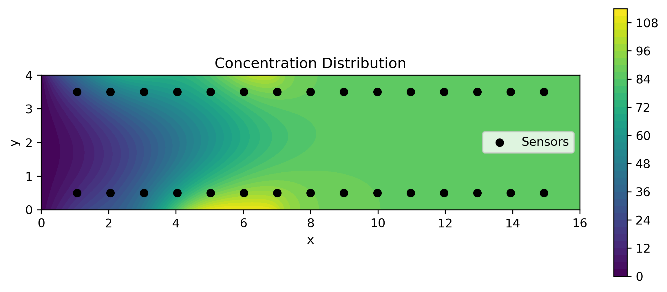
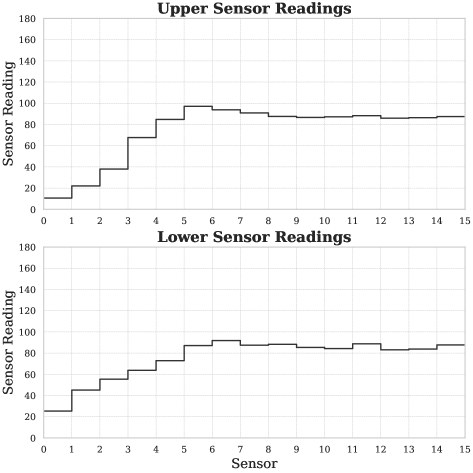
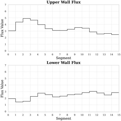
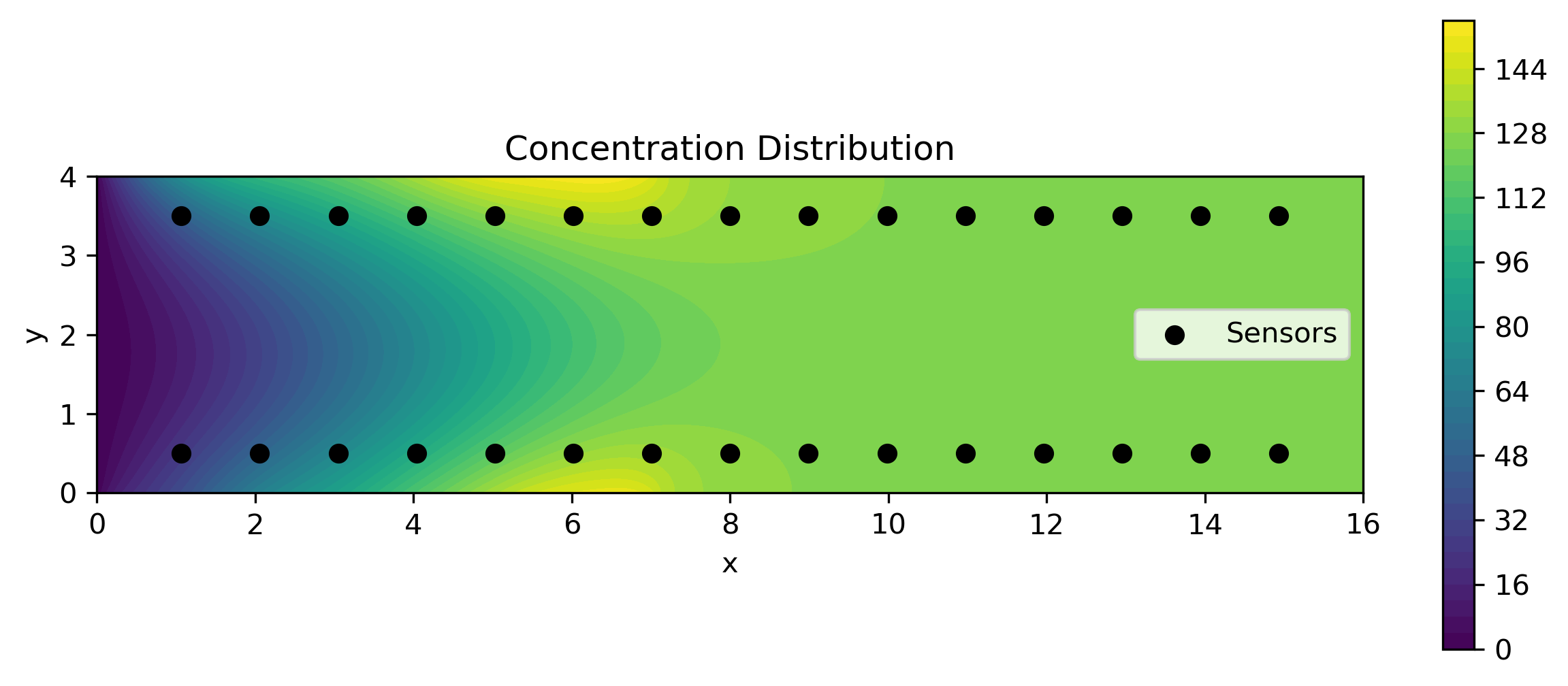
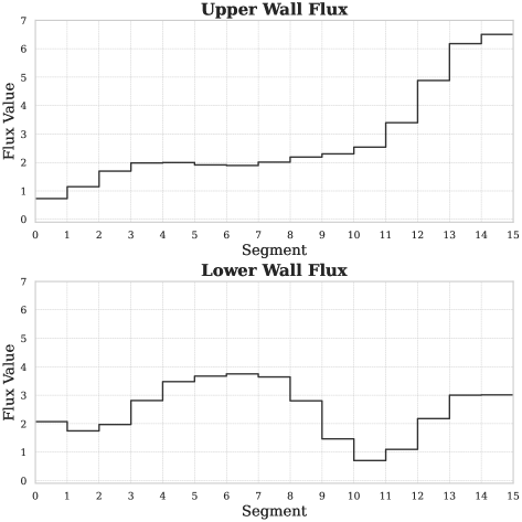
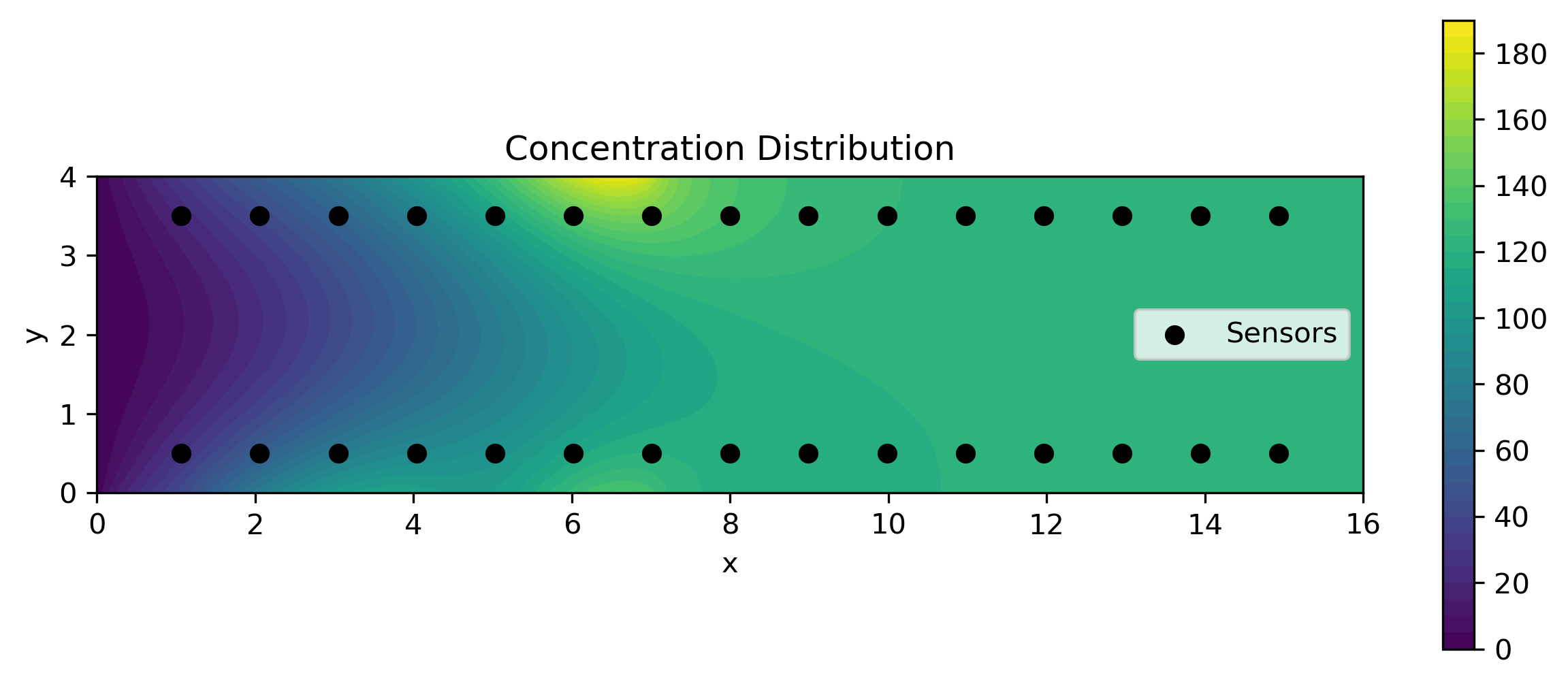
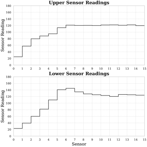
Figure 5: Three realizations of the top and bottom wall flux (${\mathbf{X}}$) sampled from the prior (first column), corresponding concentration fields obtained after solving (52), and corresponding measurements (${\mathbf{Y}}$) at various sensor locations (third column)

For a given level of measurement noise, 9,000 instances of ${\mathbf{X}}$ and ${\mathbf{Y}}$ were used to train the score networks for the variance exploding and preserving formulations. Thereafter, for each measurement from the test set, 1000 samples of the inferred flux (that belong to the posterior distribution) were generated. Sampling was performed using both the ODE and the SDE sampler. The difference between the two sampling methods was minimal and therefore only results for the ODE sampler were reported.

In Fig. 6, we present results for the variance exploding formulation with measurement noise $\sigma_{\epsilon}=0.02$ for three test cases. For each case, we plot the true flux distribution, the empirical mean generated by the conditional diffusion model (considered to be the best guess), and the one standard deviation range about the mean. In each case, we observe that mean is close to the true value, and that in most cases the true value is contained within the one standard deviation range of the mean.

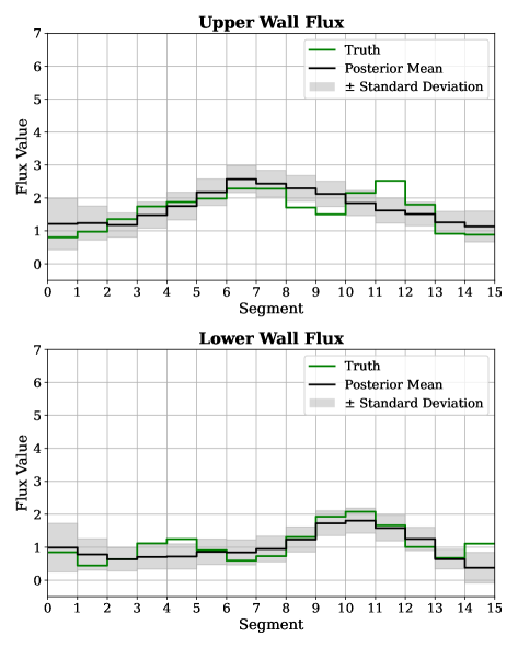
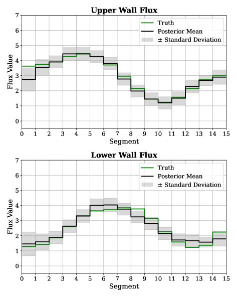
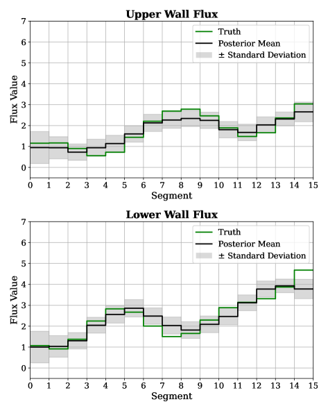
Figure 6: Posterior mean of boundary flux ((black line)) estimated using the variance exploding formulation with the ODE sampler for each segment in the upper and lower walls for three different measurements in the test dataset, corresponding true flux values (green line), and one standard deviation range around the posterior mean (gray shade)

A quantitative measure of the difference between the predicted mean and the true flux is shown in Fig. 7. Here, for each segment, we have plotted the average of the absolute value of the difference between the mean predicted flux and the true flux. The average is taken across all test samples. Further, this value is normalized by the average value of flux for all segments and all samples in the test set. Thus, a value of 0.1 for the error implies a discrepancy of around 10% between the predicted mean and the true value of the flux. Several interesting trends are observed in this plot.

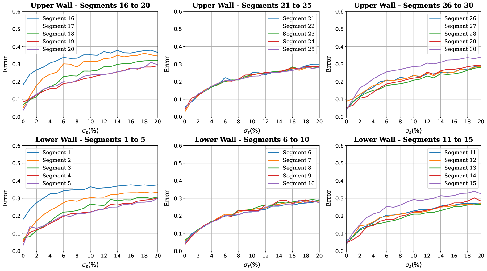
Figure 7: Sample-averaged absolute error of the generated posterior mean flux at each segment of the lower and the upper wall, normalized by the average value of flux, for all segments and all samples in the test set, for different levels of measurement noise. These results were obtained using the variance exploding formulation and ODE sampler

First, for every segment, the error increases with increasing standard deviation in measurement noise. This is to be expected, since for the same signal magnitude, increasing the magnitude of noise makes the measurements less informative and thereby increases the prediction error. Second, even with zero measurement noise, there is significant error in the prediction (around 5.9%). This is attributed to the fact that the measurements are sparse (only 30 points in the entire domain) and the inverse problem is likely ill-posed even in the absence of noise. Third, the error in predicting the flux for the first segment (both at the bottom and the top) is larger than that for the other segments. This can be explained by recognizing that all flux segments are informed by both upstream and downstream measurements (see Fig. 4), except for the first segment at the upper and lower walls which are informed only by downstream measurements. This is the likely cause for larger error for these segments. Finally, we note that the error appears to saturate with increasing noise. This is because with increasing noise the measurements cease to be informative and the posterior distribution reverts to the prior for every level of noise.

In Fig. 8, we plot similar results for the variance preserving formulation. By comparing this figure with Fig. 7, we note that the two formulations incur similar errors.

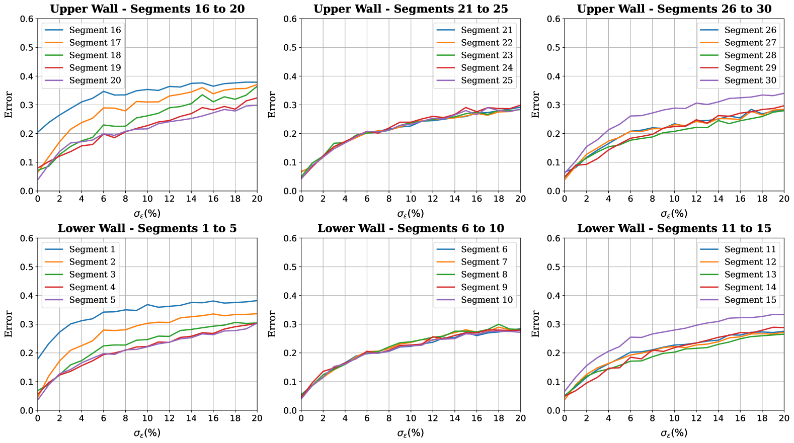
Figure 8: Sample-averaged absolute error of the generated posterior mean flux at each segment of the lower and the upper wall, normalized by the average value of flux, for all segments and all samples in the test set, for different levels of measurement noise. These results were obtained using the variance preserving formulation and ODE sampler

In Figs. 9 and 10 we plot the average value of the standard deviation of the predicted flux computed using the variance exploding and preserving formulations, respectively. In these figures, the dashed horizontal lines denote the standard deviation of the flux across all test samples. This value approximates the standard deviation of the prior distribution for the flux for each segment. We observe that with increasing measurement noise, the standard deviation of the posterior distribution increases, and at high levels of noise it approaches the standard deviation of the prior distribution once again underlining the fact that at these levels the noise in the measurement makes them uninformative and posterior distribution defaults to the prior distribution.

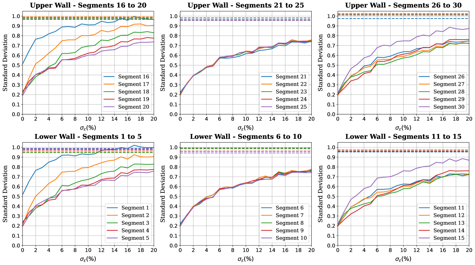
Figure 9: Sample-averaged posterior standard deviation of the flux for each segment of the lower and the upper wall for different levels of measurement noise obtained using the variance exploding formulation and ODE sampler

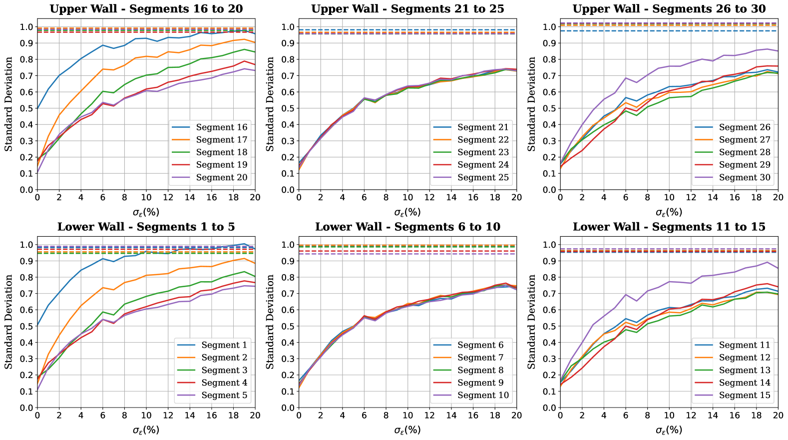
Figure 10: Sample-averaged posterior standard deviation of the flux for each segment of the lower and the upper wall for different levels of measurement noise obtained using the variance preserving formulation and ODE sampler

5.2.1 Multiple measurement operators

Next, we demonstrate how a single diffusion model can be trained to handle multiple measurement operators. The theoretical development for this is described in Section 3. We parameterize the distribution of measurement operators by a ${n_{\mathcal{Y}}}$-dimensional binary variable ${\mathbf{M}}$. We define ${\mathbf{M}}$ as follows

$$M_{i}=\left\{\begin{array}[]{cc}1&\mbox{if the $i$th sensor is on}\\ 0&\mbox{if the $i$th sensor is off.}\end{array}\right.$$ (53)

For the marginal distribution of ${\mathbf{M}}$ we select each $M_{i}$ to be an independent Bernoulli variable with $p=0.7$, that is, the probability of any sensor being on is 70%.

As described in Section 3.1, we generate the training data by sampling ${\mathbf{m}}$ from its marginal, ${\mathbf{x}}$ from its prior, and then solving (52) to determine the concentration field. Thereafter, we sample the concentration field at the locations where the sensor is on and set the measurement to the concentration plus an additive Gaussian noise. For locations where the sensor is off, we set the concentrations to -1.

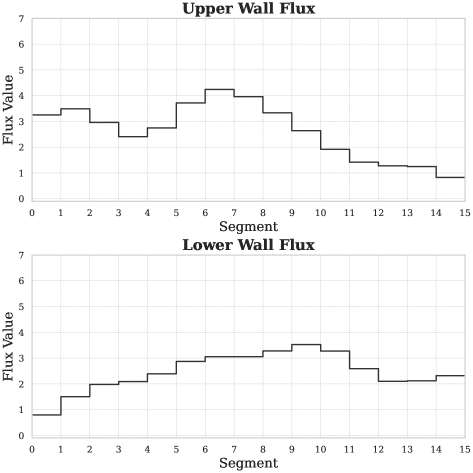
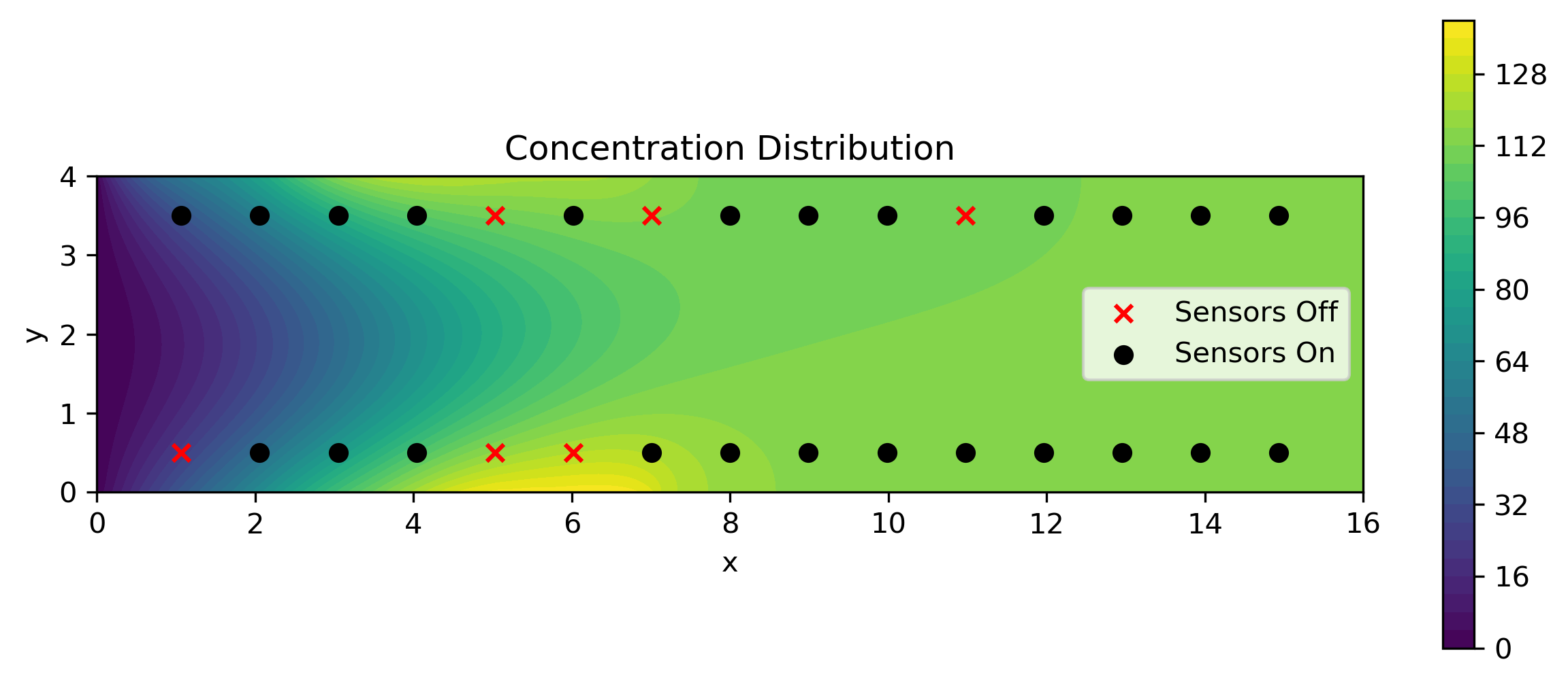
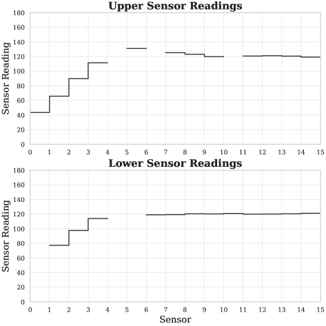
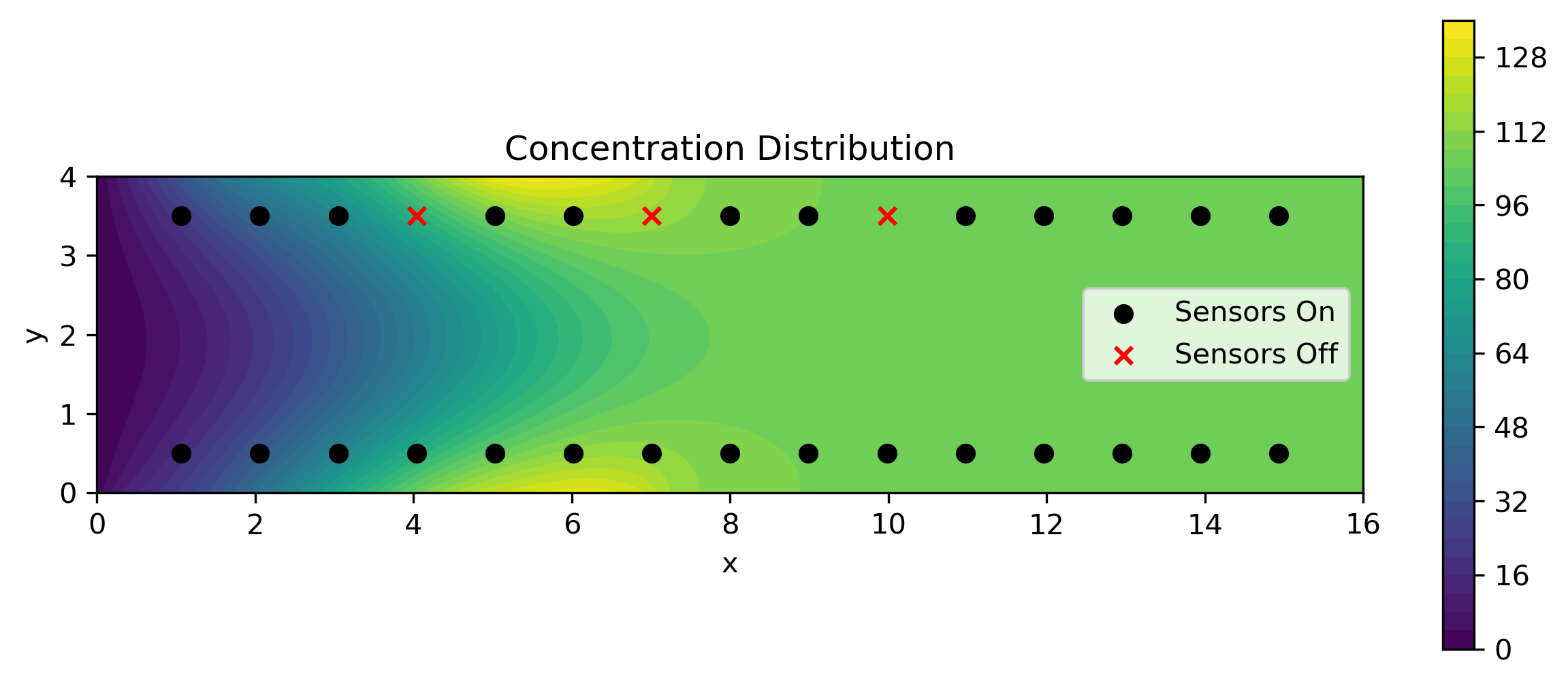
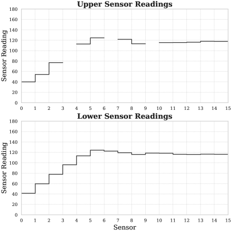
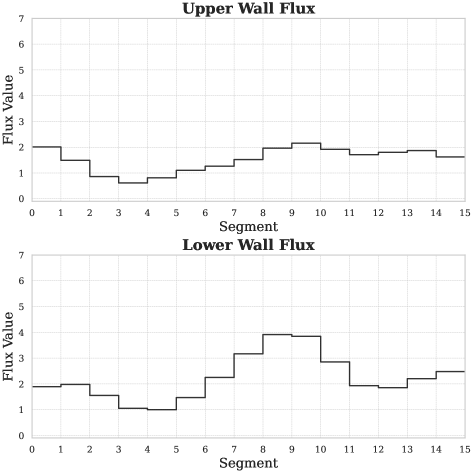
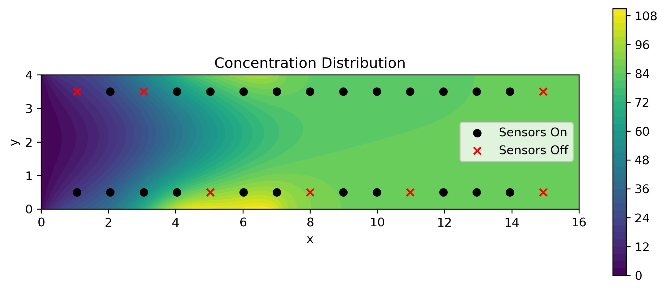
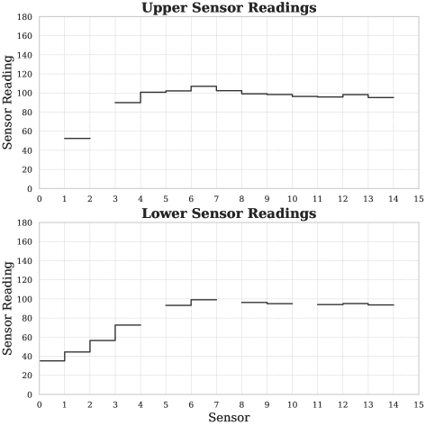
Figure 11: Three realizations of the top and bottom wall flux (${\mathbf{X}}$) sampled from the prior (first column), corresponding concentration fields obtained after solving (52), and corresponding concentration measurements (${\mathbf{Y}}$) at various sensor locations (third column) when sensors are ON with 70% probability. Red crosses ($\times$) are used to denote sensors that are OFF, which are also reflected by gaps in the concentration profiles

Using the training dataset, which consists of 36,000 realizations from the joint distribution of ${\mathbf{X}}$,${\mathbf{Y}}$ and ${\mathbf{M}}$, we train a score network whose input includes ${\mathbf{x}}$, ${\mathbf{y}}$, ${\mathbf{m}}$ and $t$. We do this for both the variance exploding and preserving formulations. We also include a plot of the spatial distribution of the concentration, which the sensors that are turned off are denoted by a red cross. Once again, we find that the results for the two formulations are similar, and thus only show results for the variance exploding formulation.

In Fig. 12, we plot results for $\sigma_{\epsilon}=0.02$, for three test cases. For each case, we plot the true flux distribution, the empirical mean generated by the conditional diffusion model (considered to be the best guess), and the one standard deviation range about the mean. Once gain, for each case, we observe that mean is close to the true value, and that in most cases the true value is contained within the one standard deviation of the mean.

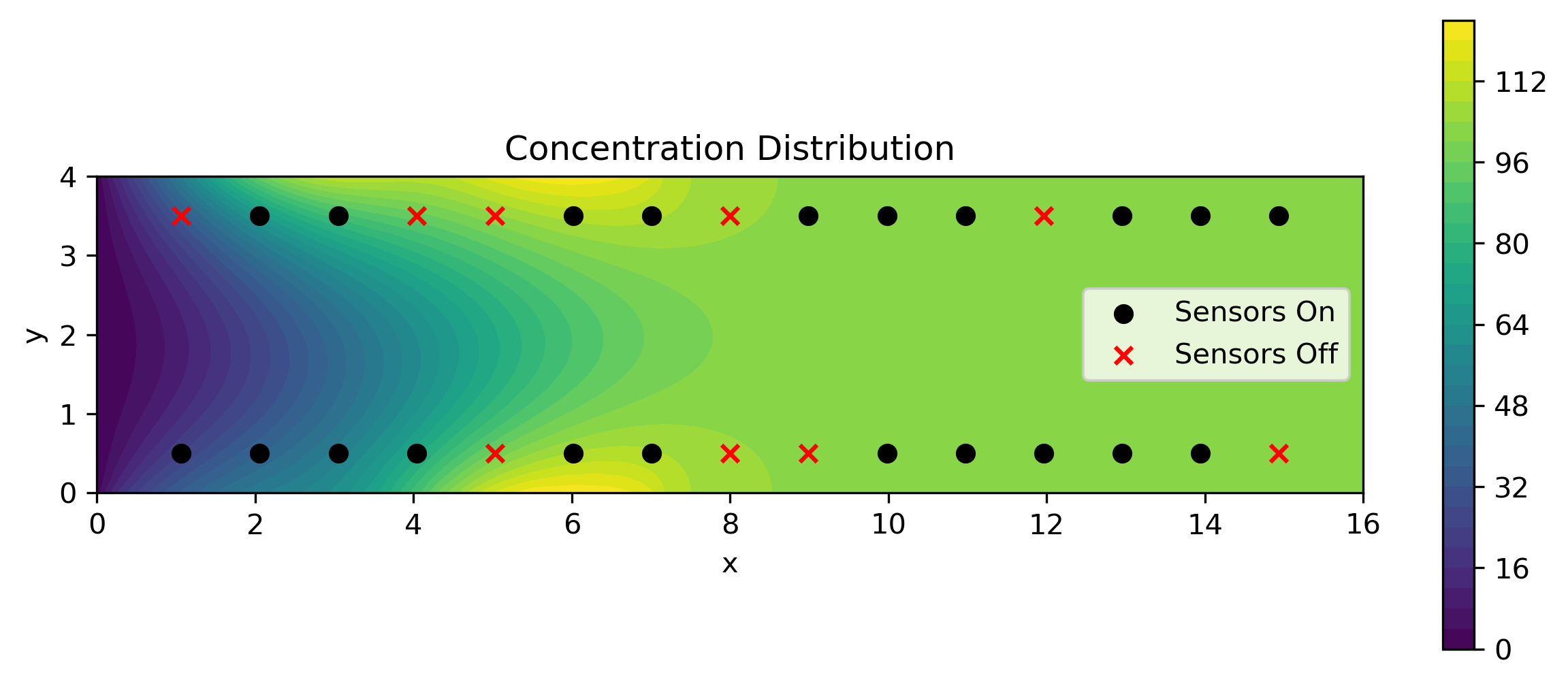
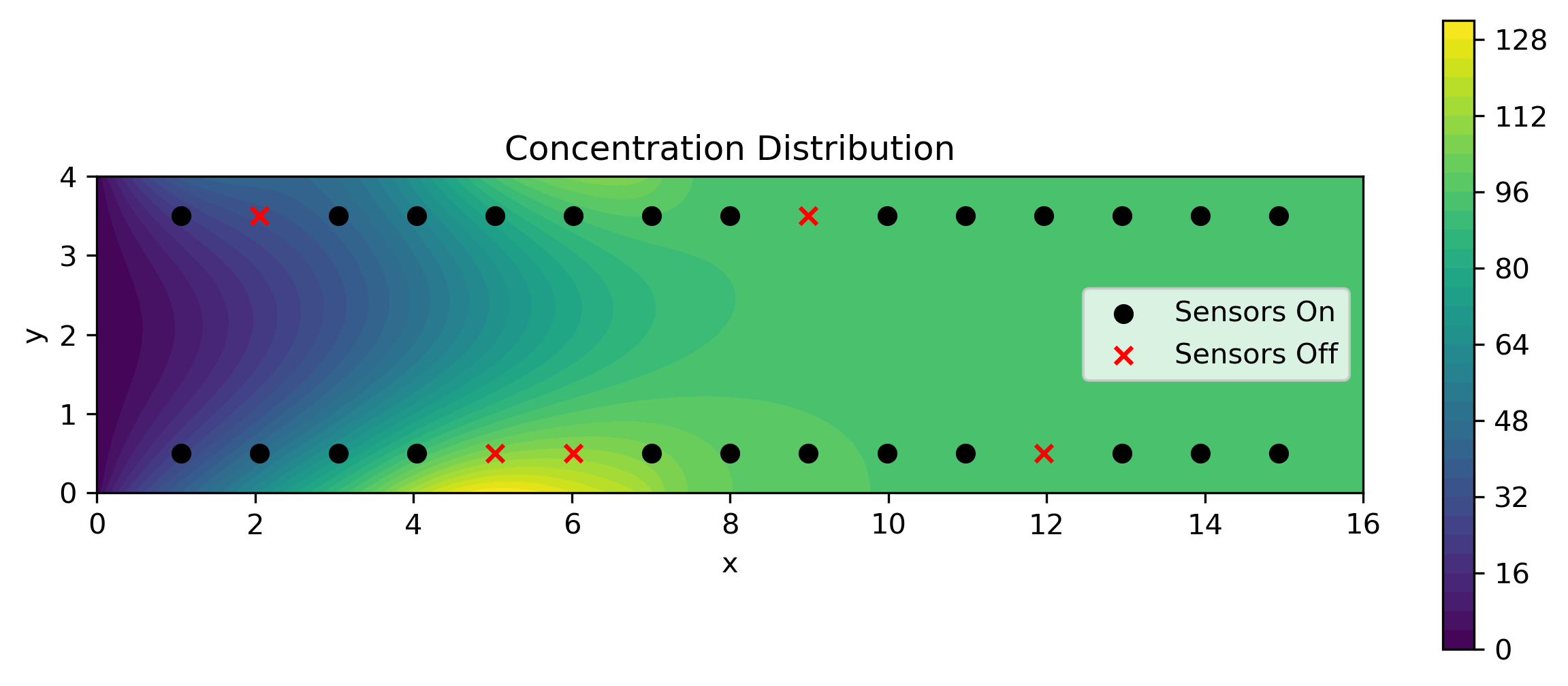
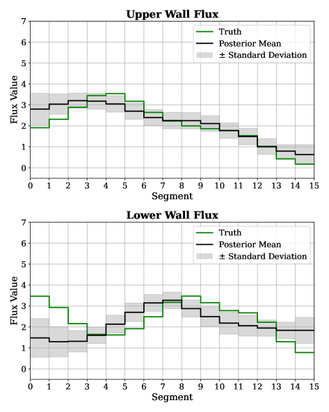
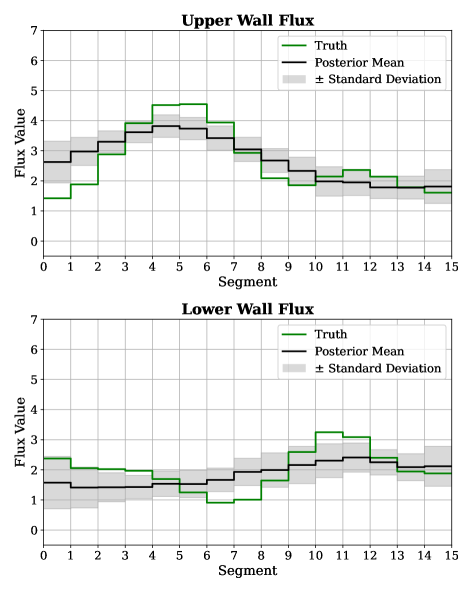
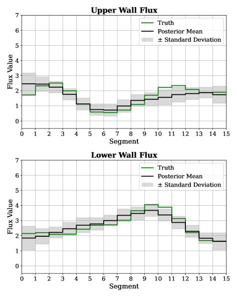
Figure 12: Posterior mean of boundary flux estimated using the variance exploding formulation with the ODE sampler for each segment in upper and lower walls for three different measurements in the test dataset (black line), true flux values (green line), one-standard deviation range around generated posterior mean (gray shade). The corresponding concentration field and sensor locations are also shown for reference (first row) with $\times$ indicating sensors that are OFF

In Fig. 13, we present a quantitative measure of the difference between the mean and the true value. For each flux segment, we plot the average of absolute value of the difference between the predicted mean and the true flux, where the average is taken across all test samples. Once again this value is normalized by the average value of flux for all segments and all samples in the test set. The trends in this plots are similar to those in Fig. 7. However, in general we observe that error in this case is higher. This is to be expected, since on average we are now working with 30% fewer measurements.

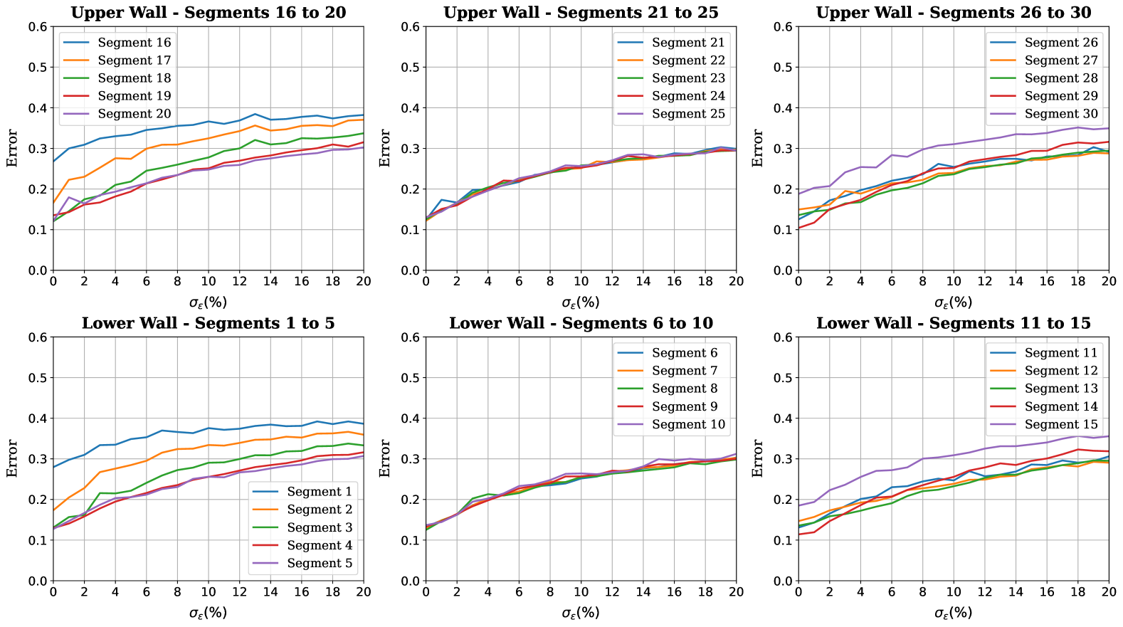
Figure 13: Sample-averaged absolute error of the generated posterior mean flux at each segment of the lower and the upper wall, normalized by the average value of flux, for all segments and all samples in the test set, for different levels of measurement noise when approximately 30% of the sensors are OFF. These results were obtained using the variance exploding formulation and ODE sampler

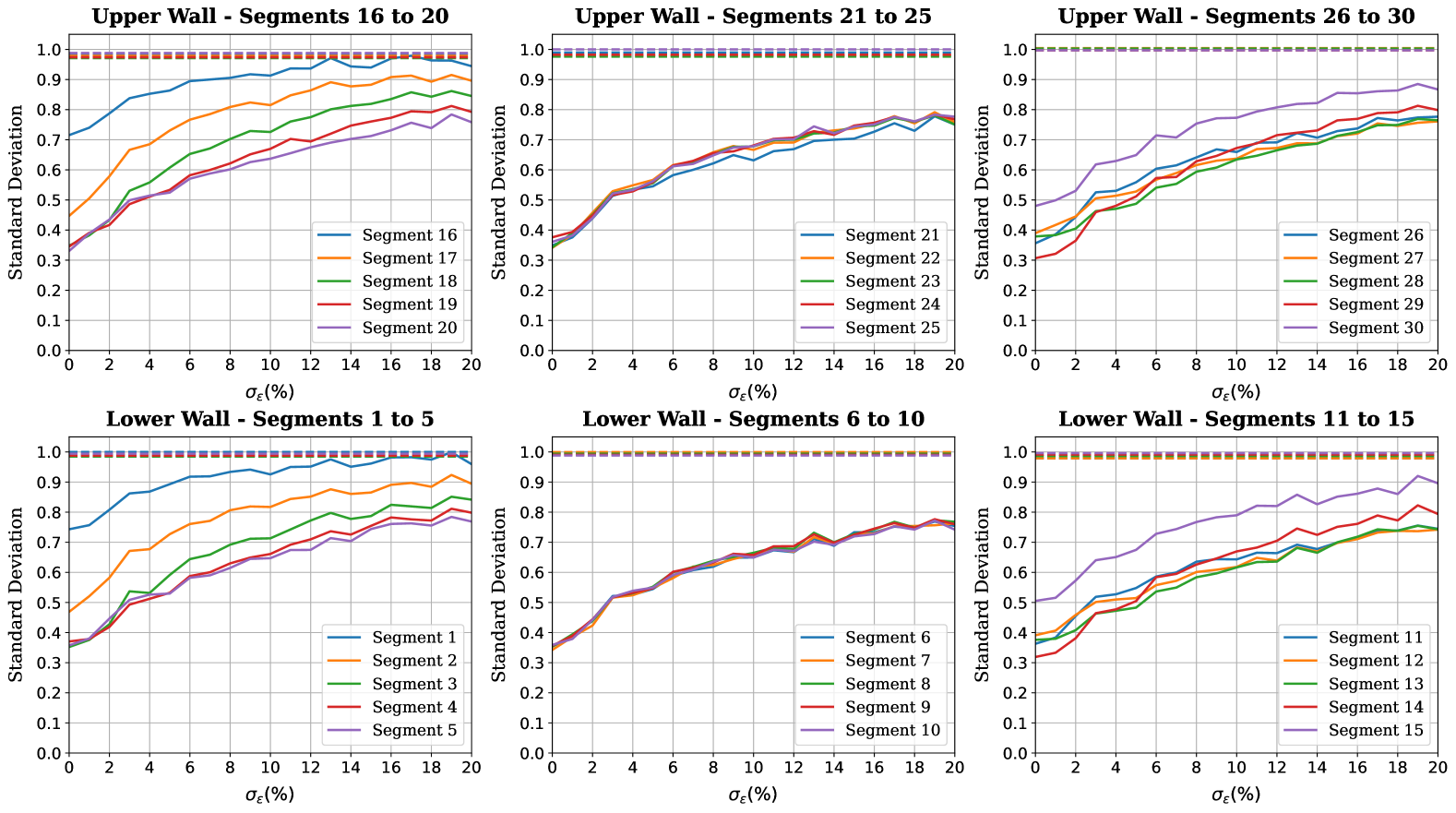
Figure 14: Sample-averaged posterior standard deviation of the flux for each segment of the lower and the upper wall for different levels of measurement noise obtained using the variance exploding formulation and ODE sampler when the measurement vector ${\mathbf{M}}$ is a random variable

6 Conclusions

In this paper we have introduced several novel concepts in the development and application of diffusion models for solving probabilistic inverse problems. By adopting a pdf-centric view of the diffusion process, we provide a constructive derivation of the reverse process that maps a reference Gaussian distribution to a complex pdf. This includes deriving the existing variance exploding and variance preserving formulations as special cases, and also deriving a new family of variance preserving formulations that are yet to be tested. Further, it identifies a family of sampling algorithms that can be used to transform samples from the reference Gaussian distribution to the underlying data distribution of which the probability flow ode is a special case.

We also consider the application of diffusion models to conditional estimation and the solution of physics-driven probabilistic inverse problems. For several low-dimensional cases we use diffusion models to generate samples from conditional distributions and quantify the error in the generated samples. In doing so, we establish a useful benchmark for these algorithms. Thereafter, we apply the conditional diffusion model to determine the boundary flux of a chemical species from sparse and noisy measurements of the interior concentration in an advection-diffusion problem. In the context of this problem, we describe how a single diffusion model can be trained to effectively solve the inverse problem associated with multiple observation operators.

Taken together, the developments of this study provide a deeper understanding of the derivation of diffusion models and their application to physics-driven probabilistic inverse problems.

7 Acknowledgments

The authors acknowledge support from ARO grant W911NF2410401. AMDC was supported in part by the Coordenacao de Aperfeicoamento de Pessoal de Nivel Superior – Brasil (CAPES) – Finance Code 001. The authors also acknowledge the Center for Advanced Research Computing (CARC, carc.usc.edu) at the University of Southern California for providing computing resources that have contributed to the research results reported within this publication.

Appendix Appendix A Experimental settings

Score network

In all our experiments, we model the score network using a deep neural network, and encode the time-dependence using the transformation:

$$f(t)=[t-0.5,\cos(2\pi t),\sin(2\pi t),-\cos(4\pi t)].$$ (54)

The time embedding $f$ is concatenated with the spatial inputs before the first hidden layer. For the advection-diffusion problem studied in Section 5.2, the measurement operator, i.e., the vector ${\mathbf{M}}$, is also concatenated with the other inputs. The missing measurements are set to $-1$. For the conditional density estimation problems in Section 5.1, the score network consists of 2 hidden layers with ReLU activation. For the advection-diffusion problem in Section 5.2, the score network consists of 4 hidden layers with ReLU activation. We optimize the score networks using Adam with a constant learning rate of ${1}\times 10^{-3}$ for 10,000 epochs and batch size equal to 1000.

Variance Schedules

We set $T=1$ in all experiments. For the variance exploding schedule, we adopt $\gamma(t)=\sigma_{\mathrm{max}}^{2t}$ such that $\sigma^{2}(t)=\left(\sigma_{\mathrm{max}}^{2t}-1\right)/\log\sigma^{2}_{\mathrm{max}}$. For the variance preserving schedule, we choose $\beta(t)=\beta_{\mathrm{min}}+t(\beta_{\mathrm{max}}-\beta_{\mathrm{min}})$. Both these schedules have been commonly adopted in the literature [28, 29, 14].

Table A1: Variance scheduling hyper-parameters for the numerical experiments in Section 5

Hyper-parameter	Conditional estimation Section 5.1	Advection-diffusion Section 5.2
$\sigma_{\mathrm{max}}$	5	5
$\beta_{\mathrm{min}}$	0.001	0.001
$\beta_{\mathrm{max}}$	5	5

Integrating the reverse process

We use an adaptive Explicit Runge-Kutta method of order 5(4), available through SciPy’s [30] solve_ivp routine to integrate Eq. 42 when $\alpha=0$. We integrate Eq. 42 using an explicit Euler-Maruyama method with $\Delta\tau=0.002$ [31] when $\alpha=1$.

References

- Bastek et al. [2024] J.-H. Bastek, W. Sun, D. M. Kochmann, Physics-informed diffusion models, arXiv preprint arXiv:2403.14404 (2024).
- Jacobsen et al. [2025] C. Jacobsen, Y. Zhuang, K. Duraisamy, Cocogen: Physically consistent and conditioned score-based generative models for forward and inverse problems, SIAM Journal on Scientific Computing 47 (2025) C399–C425.
- Dasgupta et al. [2025] A. Dasgupta, H. Ramaswamy, J. Murgoitio-Esandi, K. Y. Foo, R. Li, Q. Zhou, B. F. Kennedy, A. A. Oberai, Conditional score-based diffusion models for solving inverse elasticity problems, Computer Methods in Applied Mechanics and Engineering 433 (2025) 117425.
- Shu and Farimani [2024] D. Shu, A. B. Farimani, Zero-shot uncertainty quantification using diffusion probabilistic models, arXiv preprint arXiv:2408.04718 (2024).
- Zhuang et al. [2025] Y. Zhuang, S. Cheng, K. Duraisamy, Spatially-aware diffusion models with cross-attention for global field reconstruction with sparse observations, Computer Methods in Applied Mechanics and Engineering 435 (2025) 117623.
- Feng et al. [2023] B. T. Feng, J. Smith, M. Rubinstein, H. Chang, K. L. Bouman, W. T. Freeman, Score-based diffusion models as principled priors for inverse imaging, in: Proceedings of the IEEE/CVF International Conference on Computer Vision, 2023, pp. 10520–10531.
- Sun et al. [2024] Y. Sun, Z. Wu, Y. Chen, B. T. Feng, K. L. Bouman, Provable probabilistic imaging using score-based generative priors, IEEE Transactions on Computational Imaging (2024).
- Tashiro et al. [2021] Y. Tashiro, J. Song, Y. Song, S. Ermon, CSDI: Conditional score-based diffusion models for probabilistic time series imputation, Advances in Neural Information Processing Systems 34 (2021) 24804–24816.
- Chung et al. [2022a] H. Chung, J. Kim, M. T. Mccann, M. L. Klasky, J. C. Ye, Diffusion posterior sampling for general noisy inverse problems, arXiv preprint arXiv:2209.14687 (2022a).
- Chung et al. [2022b] H. Chung, B. Sim, D. Ryu, J. C. Ye, Improving diffusion models for inverse problems using manifold constraints, Advances in Neural Information Processing Systems 35 (2022b) 25683–25696.
- Graikos et al. [2022] A. Graikos, N. Malkin, N. Jojic, D. Samaras, Diffusion models as plug-and-play priors, Advances in Neural Information Processing Systems 35 (2022) 14715–14728.
- Mardani et al. [2023] M. Mardani, J. Song, J. Kautz, A. Vahdat, A variational perspective on solving inverse problems with diffusion models, arXiv preprint arXiv:2305.04391 (2023).
- Song and Ermon [2019] Y. Song, S. Ermon, Generative modeling by estimating gradients of the data distribution, Advances in Neural Information Processing Systems 32 (2019).
- Song et al. [2021] Y. Song, J. Sohl-Dickstein, D. P. Kingma, A. Kumar, S. Ermon, B. Poole, Score-based generative modeling through stochastic differential equations, International Conference on Learning Representations 31 (2021).
- Ho et al. [2020] J. Ho, A. Jain, P. Abbeel, Denoising diffusion probabilistic models, Advances in Neural Information Processing Systems 33 (2020) 6840–6851.
- Batzolis et al. [2021] G. Batzolis, J. Stanczuk, C.-B. Schönlieb, C. Etmann, Conditional image generation with score-based diffusion models, arXiv preprint arXiv:2111.13606 (2021).
- Song and Ermon [2020] Y. Song, S. Ermon, Improved techniques for training score-based generative models, Advances in Neural Information Processing Systems 33 (2020) 12438–12448.
- Song et al. [2021] Y. Song, L. Shen, L. Xing, S. Ermon, Solving inverse problems in medical imaging with score-based generative models, arXiv preprint arXiv:2111.08005 (2021).
- Song et al. [2022] J. Song, A. Vahdat, M. Mardani, J. Kautz, Pseudoinverse-guided diffusion models for inverse problems, in: International Conference on Learning Representations, 2022.
- Daras et al. [2024] G. Daras, H. Chung, C.-H. Lai, Y. Mitsufuji, J. C. Ye, P. Milanfar, A. G. Dimakis, M. Delbracio, A survey on diffusion models for inverse problems, arXiv preprint arXiv:2410.00083 (2024).
- Hyvärinen and Dayan [2005] A. Hyvärinen, P. Dayan, Estimation of non-normalized statistical models by score matching, Journal of Machine Learning Research 6 (2005).
- Stuart [2010] A. M. Stuart, Inverse problems: a bayesian perspective, Acta numerica 19 (2010) 451–559.
- Paszke et al. [2019] A. Paszke, S. Gross, F. Massa, A. Lerer, J. Bradbury, G. Chanan, T. Killeen, Z. Lin, N. Gimelshein, L. Antiga, A. Desmaison, A. Kopf, E. Yang, Z. DeVito, M. Raison, A. Tejani, S. Chilamkurthy, B. Steiner, L. Fang, J. Bai, S. Chintala, PyTorch: An imperative style, high-performance deep learning library, in: Advances in Neural Information Processing Systems, 2019, pp. 8024–8035.
- Ray et al. [2023] D. Ray, J. Murgoitio-Esandi, A. Dasgupta, A. A. Oberai, Solution of physics-based inverse problems using conditional generative adversarial networks with full gradient penalty, Computer Methods in Applied Mechanics and Engineering 417 (2023) 116338.
- Cuturi [2013] M. Cuturi, Sinkhorn distances: Lightspeed computation of optimal transport, Advances in Neural Information Processing Systems 27 (2013) 2292 – 2300.
- Flamary et al. [2021] R. Flamary, N. Courty, A. Gramfort, M. Z. Alaya, A. Boisbunon, S. Chambon, L. Chapel, A. Corenflos, K. Fatras, N. Fournier, L. Gautheron, N. T. Gayraud, H. Janati, A. Rakotomamonjy, I. Redko, A. Rolet, A. Schutz, V. Seguy, D. J. Sutherland, R. Tavenard, A. Tong, T. Vayer, Pot: Python optimal transport, Journal of Machine Learning Research 22 (2021) 1–8. URL: http://jmlr.org/papers/v22/20-451.html.
- Logg et al. [2012] A. Logg, K.-A. Mardal, G. N. Wells, et al., Automated Solution of Differential Equations by the Finite Element Method, Springer, 2012. doi:10.1007/978-3-642-23099-8.
- Baptista et al. [2025] R. Baptista, A. Dasgupta, N. B. Kovachki, A. Oberai, A. M. Stuart, Memorization and regularization in generative diffusion models, arXiv preprint arXiv:2501.15785 (2025).
- Karras et al. [2022] T. Karras, M. Aittala, T. Aila, S. Laine, Elucidating the design space of diffusion-based generative models, Advances in Neural Information Processing Systems 35 (2022) 26565–26577.
- Virtanen et al. [2020] P. Virtanen, R. Gommers, T. E. Oliphant, M. Haberland, T. Reddy, D. Cournapeau, E. Burovski, P. Peterson, W. Weckesser, J. Bright, S. J. van der Walt, M. Brett, J. Wilson, K. J. Millman, N. Mayorov, A. R. J. Nelson, E. Jones, R. Kern, E. Larson, C. J. Carey, İ. Polat, Y. Feng, E. W. Moore, J. VanderPlas, D. Laxalde, J. Perktold, R. Cimrman, I. Henriksen, E. A. Quintero, C. R. Harris, A. M. Archibald, A. H. Ribeiro, F. Pedregosa, P. van Mulbregt, SciPy 1.0 Contributors, SciPy 1.0: Fundamental Algorithms for Scientific Computing in Python, Nature Methods 17 (2020) 261–272. doi:10.1038/s41592-019-0686-2.
- Kloeden et al. [2012] P. E. Kloeden, E. Platen, H. Schurz, Numerical solution of SDE through computer experiments, Springer Science & Business Media, 2012.