Adaptive Multirobot Virtual Structure Control using Dual Quaternions

Abstract

A dual quaternion-based control strategy for formation flying of small UAV groups is proposed. Through the definition of a virtual structure, the coordinated control of formation’s position, orientation, and shape parameters is enabled. This abstraction simplifies formation management, allowing a low-level controller to compute commands for individual UAVs. The controller is divided into a pose control module and a geometry-based adaptive strategy, providing efficient and precise task execution. Simulation and experimental results validate the approach.

1 INTRODUCTION

A key area of recent interest is the control and coordination of multiple Unmanned Aerial Vehicles (UAVs) in formation. Formation control enables groups of UAVs to maintain specific geometric arrangements while performing tasks, offering advantages such as enhanced coverage, efficiency, and redundancy [12]. These benefits are critical for applications ranging from search and rescue to cooperative tasks like cargo transport and aerial cinematography. In cargo transportation, for instance, distributing payloads across multiple UAVs allows the delivery of heavier loads, especially in remote or disaster-affected areas. In aerial filming, coordinated UAVs can capture dynamic multi-angle footage, revolutionizing creative possibilities in the entertainment industry.

This paper introduces a dual quaternion-based control strategy for the formation flight of small UAV groups. The approach leverages a virtual structure to manage the position and orientation of the formation, simplifying task coordination. This method is particularly effective for cooperative tasks where small groups of UAVs are employed. Unlike traditional approaches, this strategy treats the formation’s shape variables as parameters, enabling adaptable control of the UAVs’ poses.

By abstracting formation control into a virtual structure, operators can command the position, orientation, and geometric parameters of the formation intuitively. For instance, a triangular formation of three UAVs can be controlled via its center and spatial orientation, reducing operational complexity. While this architecture addresses many practical challenges, limitations such as singularities in certain formations or transitions between different geometries are considered.

Unlike [9, 7, 5, 8], this work proposes a control strategy based on dual quaternions, which adapts the gains to the robot formation’s geometry, improving tracking performance. Additionally, by introducing a partial representation of the pose of the robot formation, we demonstrate how it is possible to handle structures where the formation’s pose is not fully defined, without requiring modifications to the controller’s structure. These results are validated through simulations and experimental results.

2 DUAL QUATERNIONS

Accurate pose representation is crucial for robots to perform complex tasks efficiently and interact intelligently with their environment. In applications such as UAVs, and mobile robots teleoperation, precise representations of the pose, is indispensable for effective route planning and safe navigation in dynamic environments.

The Newton-Euler equations traditionally separate translational and rotational motions, leading to control laws for 3+3-DOF motion. However, dual quaternions unify these motions into a compact framework, simplifying the design of control laws for full 6-DOF motion. This unified approach is especially beneficial in underactuated systems, such as multirotors or fixed-wing aircraft, where translational and rotational motions are strongly coupled.

Dual quaternions provide a numerically stable representation of Euclidean transformations due to their smaller solution space co-dimension and direct normalization process, ensuring stability during integration.

2.1 Quaternions

Quaternions can be thought of as a four-dimensional generalization of the complex numbers defined as:

$$H:= \{\overline{q}=q_{0}+q_{1}i+q_{2}j+q_{3}k\mid q_{i}\in\mathbb{R},$$

$$\,i^{2}=j^{2}=k^{2}=ijk=-1\},$$

where multiplication is non-commutative. Every quaternion $\overline{q}\in H$ has a real and imaginary part, denoted as $q_{0}$ and $q$, respectively. Analogously to the complex numbers, its conjugate can be defined for $\overline{q}=q_{0}+q_{1}i+q_{2}j+q_{3}k$:

$$\overline{q}^{*}=q_{0}-q_{1}i-q_{2}j-q_{3}k,$$

so that $\overline{q}\overline{p}=\overline{p}^{*}\overline{q}^{*}$, and its norm as $\|\overline{q}\|=\sqrt{\overline{q}\overline{q}^{*}}$. The inverse of $\overline{q}\neq 0$ is $\overline{q}^{-1}={\overline{q}^{*}}/{\|\overline{q}\|^{2}}$.

In particular, the set of unit quaternions $H_{1}$ is widely used in robotics being a consistent way to represent attitude. Unit quaternions are a Lie group under multiplication. The inverse of multiplication is reduced to conjugation and the unit is the real quaternion $1$. To each element in $H_{1}$ it is possible to assign an element in $SO(3)$:

$$R:H_{1}\to SO(3),\quad\overline{q}\mapsto R(\overline{q})=I_{3}+2q_{0}({q}\times)+2({q}\times)^{2},$$

where $(\cdot)\times:\mathbb{R}^{3}\to\text{so}(3)$ is the standard map of vectors to skew-symmetric $3\times 3$ matrices. This formula is a two to one map given that $R(\overline{q})=R(-\overline{q})$.

The Lie algebra of unit quaternions is the set of purely imaginary quaternions, i.e., $h_{1}=\left\{\overline{q}\in H:\overline{q}=0+{q}\right\}$. Every $\overline{q}\in h_{1}$ is univocally related with one element $q\in\mathbb{R}^{3}$. Given $x\in\mathbb{R}^{3}$, we denote $\overline{x}\in h_{1}$ as the quaternion with zero real part, and imaginary part equal to $x$. In a similar way, for $\overline{q}\in h_{1}$, the inverse of this map is denoted as ${q}\in\mathbb{R}^{3}$.

Also, given $x\in\mathbb{R}^{3}$, it is possible to assign an element in $H_{1}$, as: $\exp(x)=C(\|{x}\|)+\frac{S(\|{x}\|)}{\|{x}\|}{x}=C\left({\theta}/{2}\right)+S\left({\theta}/{2}\right){n},$ where ${n}\in\mathbb{R}^{3}$ is a unit vector representing the axis of rotation and $\theta$ is the angle of rotation.

For quaternions $v\in h_{1}$ and $\overline{q}\in H_{1}$, the Adjoint transformation is defined as $Ad_{\overline{q}}\overline{x}=\overline{q}\,\overline{x}\,\overline{q}^{*}$.

Given the angular velocity $\overline{\omega}\in h_{1}$, the kinematic equation of a rigid-body is given by

$$\dot{\overline{q}}=\frac{1}{2}\overline{q}\,\overline{\omega}.$$ (1)

2.2 Dual Quaternions and Unit Dual Quaternions

Dual numbers are a generalization of real numbers [2]. They are defined as

$$D:=\left\{x=x_{P}+\varepsilon x_{D}\mid x_{P},x_{D}\in\mathbb{R},\,\varepsilon^{2}=0\right\},$$

with $x_{P}$ being the principal part and $x_{D}$ being the dual part. The addition and multiplication can be easily extended from real numbers considering $\varepsilon^{2}=0$. Dual numbers structure as a commutative ring.

Dual quaternions [2] can be defined as

$$\tilde{D}=\left\{\tilde{q}=q_{P}+\varepsilon q_{D}\mid q_{P},q_{D}\in H\right\}.$$

Conjugation is naturally extended for any dual quaternion $\tilde{q}=\overline{q}_{P}+\varepsilon\overline{q}_{D}$ as ${\tilde{q}^{*}}=\overline{q}_{P}^{*}+\varepsilon\overline{q}_{D}^{*}$. So is the norm, $\|\tilde{q}\|=\sqrt{{\tilde{q}}^{*}\tilde{q}}$. Unit dual quaternions are defined as:

$$\tilde{D}_{1}=\left\{\tilde{q}\in\tilde{D}\mid\|\tilde{q}\|=1\right\},$$

they are Lie group with the inverse of a unit dual quaternion being its conjugate. Every unit dual quaternion can be written as $\tilde{q}=\overline{q}+\varepsilon\frac{1}{2}\overline{p}\,\overline{q},$ where $\overline{q}\in H_{1}$ is a unit quaternion representing a rotation and $\overline{p}\in h_{1}$ is purely imaginary quaternion representing a translation.

Given the angular velocity $\omega\in\mathbb{R}^{3}$ and the linear velocity $v\in\mathbb{R}^{3}$, the attitude kinematic equation for unit dual quaternion is given by

$$\dot{\tilde{q}}=\frac{1}{2}\tilde{q}\,\tilde{\Omega}(\omega,v),$$ (2)

where $\tilde{\Omega}(\omega,v)=\overline{\omega}+\varepsilon\,Ad_{\overline{q}^{*}}\overline{v}\in\tilde{d}_{1}$. Also given $\tilde{q}\in\tilde{D}_{1}$ and $\tilde{x}\in\tilde{d}_{1}$, the Adjoint transformation is defined as $Ad_{\tilde{q}}\tilde{x}=\tilde{q}\,\tilde{x}\,\tilde{q}^{*}$. Let $\tilde{q}=\overline{q}+\frac{\varepsilon}{2}\overline{p}\,\overline{q}\in\tilde{D}_{1}$, and $\tilde{x}=\overline{x}_{P}+\varepsilon\overline{x}_{\in}\tilde{d}_{1}$ notice that $Ad_{\tilde{q}}(\tilde{x})=Ad_{\overline{q}}\overline{x}_{P}+\varepsilon(Ad_{\overline{q}}\overline{x}_{D}+Ad_{\overline{q}}(\overline{p}\times\overline{x}_{P})).$

2.3 Applications of Quaternions and Dual Quaternions for Rigid Body Pose Representation

Suppose that $b$ and $i$ represent the body (robot) and inertial frames, respectively. Let ${\omega^{b}}\in\mathbb{R}^{3}$ denote the angular velocity of the robot with respect to $i$, expressed in the body coordinates $b$, and let $\overline{q}_{b}^{i}\in H_{1}$ be defined as in equation (1). Given ${p^{b}}\in\mathbb{R}^{3}$, the position in the body frame, if $\overline{p}=Ad_{\overline{q}_{b}^{i}}\overline{p^{b}}$, then ${p}\in\mathbb{R}^{3}$ is the robot’s position in the inertial frame. On the other hand, $\overline{q}_{i}^{b}={\overline{q}_{b}^{i}}^{*}$, and $\overline{p^{b}}=Ad_{{q}_{i}^{b}}\overline{p}$.

Now, suppose that $p$ is the position of the robot in the inertial frame. Then, $\tilde{q}_{b}^{i}=\overline{q}_{b}^{i}+\frac{\varepsilon}{2}\overline{p}\,\overline{q}_{b}^{i}$ satisfies the kinematic equation (2) with $\tilde{\Omega}(\omega,v)=\overline{\omega}^{b}+\varepsilon Ad_{\overline{q}_{i}^{b}}\overline{v},$, where $\overline{v}=\dot{\overline{p}}\in h_{1}$.

From a navigation algorithms perspective, this is a practical representation, considering a strapdown configuration where gyroscopes measure angular velocity in body frame while GPS measures position with respect to the ECEF (Earth-Centered Earth-Fixed) frame, which can be regarded as an inertial frame $i$ for many cases.

However, in some applications, it may be preferable to represent all quantities in inertial frames. In this case, if $\xi\in\mathbb{R}^{3}$ is the angular velocity that satisfies $\dot{\overline{q}_{i}^{b}}=\frac{1}{2}\overline{q}_{i}^{b}\overline{\xi}$, then $\tilde{q}_{i}^{b}=\overline{q}_{i}^{b}+\frac{\varepsilon}{2}\overline{p}^{b}\,\overline{q}_{i}^{b}\in\tilde{D}_{1}$ in this case satisfies equation (2) with $\tilde{\Omega}(\xi,v)=\overline{\xi}+\varepsilon Ad_{\overline{q}_{i}^{b}}\dot{\overline{p}^{b}}=\overline{\xi}+\varepsilon(\overline{\xi}\times\overline{p}+\overline{v}).$

2.4 Dual Quaternions and UAV formation control

The properties of dual quaternions allow for a compact representation of rigid body transformations, which is crucial in scenarios requiring precise spatial configurations. In the realm of UAVs, dual quaternions have gained prominence in formation control, where multiple UAVs must coordinate their movements to maintain a specified configuration. The use of dual quaternion algebra facilitates the management of relative positions and orientations among UAVs, thereby improving the efficiency of multi-UAV operations [4, 11]. This approach addresses significant challenges such as instability during leader-follower dynamics and the computational demands of real-time information sharing, enabling more effective control strategies in dynamic environments [3, 13]. Notable applications of dual quaternions in UAV formation control include scenarios involving cargo transportation with cable-suspended loads, where a unified framework is employed to handle both the UAV’s trajectory and the load’s dynamics. Simulations have demonstrated that UAV systems utilizing dual quaternion-based control exhibit superior performance in trajectory tracking and stability compared to traditional methods [13]. Ongoing research continues to explore the potential of dual quaternions in enhancing UAV operations, focusing on refining control algorithms, expanding their applicability to multi-robot systems, and addressing the nuances of coupling translation and rotation. As the mathematical framework evolves, it holds promise for significant advancements in both theoretical understanding and practical applications of UAV technology [6].

In [5], a dual quaternion-based control law for mobile robot coordination is introduced, incorporating integral action to reduce dynamic errors. Extensions to underactuated vehicle formations with efficient gain tuning are proposed in [8]. This work builds on these results, with additional insights into gain bounds. For brevity, detailed proofs following [8] are omitted.

Theorem 1.

Let $C\subseteq\mathbb{R}^{d}$ be a compact set and $K_{\omega,p}$, $K_{v,p}$, $K_{\omega,i}$, $K_{v,i}$, $K_{\eta}$, $K_{\xi}$ $:\mathbb{R}^{d}\rightarrow\mathbb{R}^{3\times 3}$ continuous uniformly negative matrices functions on $C$. Given the desired angular and linear velocities $\omega_{d},{v}_{d}$, and the desired dual quaternion $\tilde{q}_{d}$ satisfying equation  (2), suppose that the dual quaternion $\tilde{q}$ is given by equation (2) with

$$\overline{\omega} =Ad_{\overline{\delta q}^{*}}\overline{\omega}_{d}+sign(\delta q_{0})(K_{\omega,p}(\rho){\delta q}+\eta_{0}K_{\omega,i}(\rho){\eta}),$$ (3)

$${v} ={v}_{d}+K_{v,p}(\rho){\delta p}+K_{v,i}(\rho){\xi},$$ (4)

$$\dot{\overline{\eta}} =\frac{1}{2}{\overline{\eta}}(-|\delta q_{0}|K_{\omega,i}(\rho){\delta q}+sign(\eta_{0})K_{\eta}(\rho){\eta}),$$ (5)

$$\dot{{\xi}} =-K_{v,i}(\rho){\delta p}+K_{\xi}(\rho){\xi}.$$ (6)

Then $({\delta q},{\delta p},{\xi},{\eta})\rightarrow{0}$ a.e. for every $\rho\in C$, with error given by $\overline{\delta q}=\overline{q_{d}}^{*}\,\overline{q}$.

The next section demonstrates how this theorem can be applied to implement a cooperative control algorithm for robot formations.

3 CLUSTER SPACE CONTROL

A cluster refers to a group of robots whose states are used to compute a new aggregated cluster state, defined in the cluster space. Cluster-Space Control (CSC) [10] models the system as an articulated kinematic mechanism, allowing the selection of state variables for effective control and monitoring.

Formation motions are defined in cluster space, while individual robots are ultimately commanded. Therefore, it is crucial to establish kinematic transformations that relate the cluster space variables to those in robot space. A cluster space controller calculates compensation actions in cluster space and, using these transformations, generates control commands for individual robots.

This method allows operators to specify and monitor the system’s motion from the cluster perspective, simplifying the task by abstracting control of individual robots and actuators.

Consider a system of $n$ robots, each with $m_{i}$ degrees of freedom. The robot state vector is ${r}_{i}\in\mathbb{R}^{m_{i}}$, and the stacked state vector in robot space is ${r}\in\mathbb{R}^{m}$, where $m=\sum{i=1}^{n}m_{i}$. Each robot’s kinematics are described by $\dot{r}_{i}=f_{i}(r_{i},u_{i})$, where $u_{i}$ is the control command. In robot space, $\dot{r}=f(r,u)=(f_{1}(r_{1},u_{1}),...,f{n}(r_{n},u_{n}))$.

The cluster space state is ${c}\in\mathbb{R}^{m}$, and its relationship with the robot space is defined through forward and inverse kinematic transformations. The forward kinematic transformation is represented by $\psi$ with $\dot{c}=J(r)f(r,u)|_{\psi^{-1}(c)}$, where ${J}({r})$ is the Jacobian matrix.

In practice, cluster space variables are decomposed into two components: $c_{q}$ for the cluster’s pose (position and orientation) and $c_{g}$ for the cluster’s shape (geometric configuration). We assume the shape dynamics are unaffected by $c_{q}$, leading to:

$$\dot{c_{g}} =\Gamma(c_{g},u_{g}),\ \dot{c_{q}}=\Gamma(c_{q},c_{g},u_{q}).$$ (7)

Here, $u_{g}$ and $u_{q}$ are independent control signals for geometry and pose. Given desired trajectories ${c_{g}}_{d}$ and ${c_{q}}_{d}$, the goal is to find $u_{g}$ and $u_{q}$ such that $c_{g}\rightarrow{c_{g}}_{d}$ and $c_{q}\rightarrow{c_{q}}_{d}$.

This separation allows the CSC to maintain its structure independently of the formation that is being controlled. We demonstrate this with clusters of two and three vehicles, using a dual quaternion-based controller to manage position and orientation $c_{q}$, while adjusting the formation geometry $c_{g}$.

3.1 Three-vehicle formation

In the case of three robots (3R), the pose of the cluster can be defined as follows. Given the positions of the robots in a local frame $r_{1},r_{2},r_{3}\in\mathbb{R}^{3}$, the center of the formation is defined as $p=\frac{\sum_{i=1}^{3}r_{i}}{3}.$ The cluster’s orientation is well-defined by the arrangement of the robots. Let $R=[x\,y\,z]\in SO(3)$ be the rotation matrix which represents the attitude of the cluster, with $x=\frac{p-r_{1}}{\|p-r_{1}\|}$, $z_{1}={{(r_{2}-r_{1})}\times(r_{3}-r_{1})}$, $z=z_{1}/\|z_{1}\|$, $y={z}\times x$ (see Figure 1). If $\overline{q}$ is such that $R=R(\overline{q})$, then the pose of the cluster is defined by the dual quaternion $\tilde{q}=\overline{q}+\varepsilon\,\frac{1}{2}\overline{p}\,\overline{q}$.

Regarding the geometrical parameters of the cluster, both the relative distances $d_{2}$ and $d_{3}$ from $r_{2}$ and $r_{3}$ to $r_{1}$, as well as the angle $\alpha$ between $r_{2}-r_{1}$ and $r_{3}-r_{1}$, are used to describe it (see Figure 1). In what follows we use the notation $S{(\alpha)}=\sin{(\alpha)}$ and $C{(\alpha)}=\cos{(\alpha)}$. Observe that

$$r_{1} =3p-r_{2}-r_{3},$$ (8)

$$r_{2}-r_{1} =d_{2}(C{({\alpha}_{2})}x-S{({\alpha}_{2})}y),$$ (9)

$$r_{3}-r_{1} =d_{3}(C{({\alpha}_{3})}x+S{({\alpha}_{3})}y),$$ (10)

where $\alpha=\alpha_{2}+\alpha_{3}$, $m^{2}=\frac{d_{2}^{2}+d_{3}^{2}+2d_{2}d_{3}\,C{(\alpha)}}{4}$, and for the angles $S{(\alpha_{i})}=\frac{d_{j}}{2\,m}S{(\alpha)}$, $C{(\alpha_{i})}=\frac{d_{j}C(\alpha)+d_{i}}{2m}$. Then

$$\begin{bmatrix}r_{1}\\ r_{2}\\ r_{3}\end{bmatrix}=\begin{bmatrix}p-\frac{d_{2}C{({\alpha}_{2})}+d_{3}C{({\alpha}_{3})}}{3}x-\frac{d_{3}S{({\alpha}_{3})}-d_{2}S{({\alpha}_{2})}}{3}y\\ p+\frac{2d_{2}C{({\alpha}_{2})}-d_{3}C{({\alpha}_{3})}}{3}x-\frac{2d_{2}S{({\alpha}_{2})}+d_{3}S{({\alpha}_{3})}}{3}y\\ p+\frac{2d_{3}C{({\alpha}_{3})}-d_{2}C{({\alpha}_{2})}}{3}x+\frac{2d_{3}S{({\alpha}_{3})}+d_{2}S{({\alpha}_{2})}}{3}y\end{bmatrix},$$

To obtain the velocity commands to control the robots, the derivatives of $r_{i}$ can be calculated. In order to do that, it is useful to compute the following:

$$\frac{d}{dt}S{(\alpha_{i})} =M_{1_{ij}}\dot{d}_{i}+M_{2_{ij}}\dot{d}_{j}+M_{3_{ij}}\dot{\alpha},$$

$$\frac{d}{dt}C{(\alpha_{i})} =N_{1_{ij}}\dot{d}_{i}+N_{2_{ij}}\dot{d}_{j}+N_{3_{ij}}\dot{\alpha},$$

where

$$M_{1_{ij}}=\frac{\partial\left(\frac{d_{j}}{2m}S{(\alpha)}\right)}{\partial d_{i}} =\frac{-d_{j}S{(\alpha)\,(d_{i}+d_{j}C{(\alpha)})}}{8m^{3}}$$

$$M_{2_{ij}}=\frac{\partial\left(\frac{d_{j}}{2m}S{(\alpha)}\right)}{\partial d_{j}} =S{(\alpha)}\frac{4m^{2}-d_{j}(d_{j}+d_{i}C{(\alpha)})}{8m^{3}}$$

$$M_{3_{ij}}=\frac{\partial\left(\frac{d_{j}}{2m}S{(\alpha)}\right)}{\partial\alpha} =d_{j}\frac{4m^{2}C{(\alpha)}+d_{i}d_{j}S^{2}{(\alpha)}}{8m^{3}}$$

$$N_{1_{ij}}=\frac{\partial\left(\frac{d_{j}C(\alpha)+d_{i}}{2m}\right)}{\partial d_{j}} =\frac{4m^{2}-(d_{i}+d_{j}C{(\alpha)})^{2}}{8m^{3}}$$

$$N_{2_{ij}}=\frac{\partial\left(\frac{d_{j}C(\alpha)+d_{i}}{2m}\right)}{\partial d_{i}} =\frac{4m^{2}C{(\alpha)-(d_{i}+d_{j}C{(\alpha)})^{2}}}{8m^{3}}$$

$$N_{3_{ij}}=\frac{\partial\left(\frac{d_{j}C(\alpha)+d_{i}}{2m}\right)}{\partial\alpha} =d_{j}S{(\alpha)}\frac{-4m^{2}+d_{i}(d_{i}+d_{j}C{(\alpha)})}{8m^{3}}$$

with $(i,j)=(2,3)$ and $(i,j)=(3,2)$.

Let $\omega^{i}=R\omega$. It follows that $\dot{x}={\omega^{i}}\times x$ and $\dot{y}={\omega^{i}}\times y$. Letting $v=\dot{p}$, the relation between the formation’s twist $\tilde{\Omega}(\omega,v)$ and the robot velocities is given by:

$$3\dot{r_{1}} =3v-((C{\alpha_{2}}+d_{2}N_{1_{23}}+d_{3}N_{2_{32}})x-$$

$$(S{\alpha_{2}}+d_{2}M_{1_{23}}-d_{3}M_{2_{32}})y)\dot{d}_{2}-$$

$$((C{\alpha_{3}}+d_{2}N_{2_{23}}+d_{3}N_{1_{32}})x+(S{\alpha_{3}}+$$

$$d_{3}M_{1_{32}}-d_{2}M_{2_{23}})y)\dot{d}_{3}-((d_{2}N_{3_{23}}+d_{3}N_{3_{32}})x+$$

$$(d_{3}M_{3_{32}}-d_{2}M_{3_{23}})y)\dot{\alpha}-(d_{2}C{\alpha_{2}+d_{3}C{\alpha_{3}}})(\omega\times x)-$$

$$(d_{3}S{\alpha_{3}}-d_{2}S{\alpha_{2}})(\omega\times y),$$

$$3\dot{r_{2}} =3v+((2C{\alpha_{2}}+2d_{2}N_{1_{23}}-d_{3}N_{2_{32}})x-$$

$$(2S{\alpha_{2}}+2d_{2}M_{1_{23}}+d_{3}M_{2_{32}})y)\dot{d}_{2}+$$

$$((-C{\alpha_{3}}+2d_{2}N_{2_{23}}-d_{3}N_{1_{32}})x-(S{\alpha_{3}}+$$

$$d_{3}M_{1_{32}}+2d_{2}M_{2_{23}})y)\dot{d}_{3}+((2d_{2}N_{3_{23}}-d_{3}N_{3_{32}})x-$$

$$(d_{3}M_{3_{32}}+2d_{2}M_{3_{23}})y)\dot{\alpha}+(2d_{2}C{\alpha_{2}}-d_{3}C{\alpha_{3}})(\omega\times x)-$$

$$(d_{3}S{\alpha_{3}}+2d_{2}S{\alpha_{2}})(\omega\times y),$$

$$3\dot{r_{3}} =3v+((-C{\alpha_{2}}-d_{2}N_{1_{23}}+2d_{3}N_{2_{32}})x+$$

$$(S{\alpha_{2}}+d_{2}M_{1_{23}}+2d_{3}M_{2_{32}})y)\dot{d}_{2}+$$

$$((2C{\alpha_{3}}-d_{2}N_{2_{23}}+2d_{3}N_{1_{32}})x+(2S{\alpha_{3}}+$$

$$2d_{3}M_{1_{32}}+d_{2}M_{2_{23}})y)\dot{d}_{3}+((-d_{2}N_{3_{23}}+2d_{3}N_{3_{32}})x+$$

$$(2d_{3}M_{3_{32}}+d_{2}M_{3_{23}})y)\dot{\alpha}+(2d_{3}C{\alpha_{3}}-d_{2}C{\alpha_{2}})(\omega\times x)+$$

$$(2d_{3}S{\alpha_{3}}+d_{2}S{\alpha_{2}})(\omega\times y).$$

These equations allow to compute the relation between the velocity of each robot and the time derivatives of the cluster variables

$$\begin{bmatrix}\dot{r}_{1},\dot{r}_{2},\dot{r}_{3}\end{bmatrix}=J^{-1}(r)|_{\psi^{-1}(c)}v_{c},$$ (11)

where $v_{c}^{T}=\begin{bmatrix}v^{T},(\omega\times x)^{T},(\omega\times y)^{T},\dot{d}_{2},\dot{d}_{3},\dot{\alpha}\end{bmatrix}^{T}$. For the shape of the 3R formation, a simple proportional controller can be implemented as follows to track a set of prescribed geometry variables $d_{d2}>0$, $d_{d3}>0$ and $\alpha_{d}$:

$$(\dot{d}_{2},\dot{d}_{3},\dot{\alpha})=(k_{d}(d_{d2}-d_{2}),k_{d}(d_{d3}-d_{3}),k_{\alpha}(\alpha_{d}-\alpha)).$$

Figure 1: 3R cluster geometry.

Algorithm 1 completes the description of the dual quaternion cluster space controller (CSC) for the 3R formation.

Algorithm 1 CSC for the 3R Formation

Assumptions: Let $C\subseteq\mathbb{R}^{d}$ be a compact set, and let $K_{\omega,p}$, $K_{v,p}$, $K_{\omega,i}$, $K_{v,i}$, $K_{\eta}$, $K_{\xi}$ $:\mathbb{R}^{d}\rightarrow\mathbb{R}^{3\times 3}$ be continuous, uniformly negative-definite matrix functions on $C$. Let the gain $k_{d}>0$, and the control period $T_{q}>0$.

Input: Desired cluster attitude $\overline{q}_{d}\in H_{1}$, desired distances $d_{di}$ ($i=2,3$) between robots, desired position of the center of the formation, robot positions $r_{i}$ ($i=1,2,3$), and the desired heading of the formation.

Output: Commanded velocity vectors $v_{i}$ for robots $i=1,2,3$.

Step: Compute the current pose of the cluster $p=(r_{1}+r_{2}+r_{3})/3$, and $R(\overline{q})\in\text{SO}(3)$, with columns $x=\frac{p-r_{1}}{\|p-r_{1}\|}$, $z_{1}={(r_{2}-r_{1})\times(r_{3}-r_{1})}$, $z=z_{1}/\|z_{1}\|$ and $y=z\times x$.

Step: Compute the attitude error $\overline{\delta q}=\overline{q}_{d}^{*}\overline{q}$.

Step: Compute the controller in equations (3) - (6).

Step: Compute the $J^{-1}$ matrix of equation (11).

3.2 Two-Vehicle Formation

In the case of two robots (2R), an additional challenge arises due to the difficulty of fully defining the attitude of the cluster. Since only two angles are required to specify the orientation of the segment connecting the two robots, a complete attitude representation is unnecessary. Nevertheless, the structure of the control algorithm can be preserved by redefining the dual quaternion error to capture only the relevant angles for this particular formation. This approach allows us to adapt the result from Theorem 1 to scenarios where the orientation of the virtual structure formed by the robot formation is not fully defined.

Theorem 2.

Let $C\subseteq\mathbb{R}^{d}$ be a compact set and $K_{\omega,p}$, $K_{\omega,i}$, $K_{\eta}$ $:\mathbb{R}^{d}\rightarrow\mathbb{R}^{3\times 3}$ continuous uniformly negative definite matrices functions on $C$. Suppose that $\overline{q}\in H_{1}$ represents the attitude of the robot, and ${z_{d}}\in\mathbb{R}^{3}$ is a unit norm vector (expressed in the inertial reference frame of the problem), which represents a desired direction where the $z$-axis of the robot should be pointing, where $z=R(\overline{q})[0\,0\,1]^{T}$, and define the tracking error as $\overline{\delta q}=\delta q_{0}+{\delta q}$, where $\delta q_{0}=\frac{1+\langle{z},{z_{d}}\rangle}{\|{z}+{z_{d}}\|}$ and ${\delta q}=\frac{{z_{d}}\times{z}}{\|{z}+{z_{d}}\|}$ (for ${z}\neq-{z_{d}})$. Suppose that $\overline{q}\in H_{1}$ is given by equation (1) with:

$$\overline{\omega} =Ad_{\overline{\delta q}^{*}}\overline{\omega}_{d}+(K_{\omega,p}(\rho){\delta q}+\eta_{0}K_{\omega,i}(\rho){\eta}),$$

$$\dot{\overline{\eta}} =\frac{1}{2}{\overline{\eta}}(-|\delta q_{0}|K_{\omega,i}(\rho){\delta q}+sign(\eta_{0})K_{\eta}(\rho){\eta}),$$

where $\overline{\eta}\in H_{1}$, and $\overline{\eta}(0)=1$. Then the $z$-axis of the robot is aligned with the desired direction $z_{d}$.

Proof: Notice that this is a particular case of the dynamics given in Theorem 1, considering only the part related to orientation. Furthermore, due to how the error is defined, it follows that $\delta\overline{q}_{0}\geq 0$. Therefore, to complete the proof, it is necessary to show that if $\delta q\rightarrow 0$, then the axes $z$ and $z_{d}$ will be aligned.

Suppose that $R(\overline{q})\in SO(3)$, where its columns ${x},{y},{z}\in\mathbb{R}^{3}$ are the robot’s axes, expressed in the inertial frame. Define ${n}=\frac{{z_{d}}\times{z}}{\|{z}\times{z_{d}}\|}$. To align these two vectors, a rotation about ${n}$ with an angle $\theta$ should be applied (see Fig. 2), where ${z}\times{z_{d}}=S(\theta)\,{n}$. The components of the quaternion representing this rotation are given by:

$${n}S({\theta}/{2}) ={{z_{d}}\times{z}}/{\|{z}+{z_{d}}\|},$$ (12)

$$C({\theta}/{2}) ={\langle{z},{z}+{z_{d}}\rangle}/{\|{z}+{z_{d}}\|}.$$ (13)

Thus, the quaternion representing the rotation to align ${z}$ with ${z_{d}}$ is given by $\overline{\delta q}=\delta q_{0}+{\delta q}$, where $\delta q_{0}=\frac{1+\langle{z},{z_{d}}\rangle}{\|{z}+{z_{d}}\|}$ and ${\delta q}=\frac{{z_{d}}\times{z}}{\|{z}+{z_{d}}\|}$. If $z+z_{d}\rightarrow 0$, then $\overline{\delta q}_{0}=C\left(\frac{\theta}{2}\right)\rightarrow 0$. Also observe that if $\overline{\delta q}\rightarrow 0$, i.e., $\overline{\delta q}_{0}\rightarrow 1$, then $z\rightarrow z_{d}$. ∎

Figure 2: Axis/angle representation for the ${z}$ to ${z_{d}}$ error.

Suppose that ${r_{1}},{r_{2}}\in\mathbb{R}^{3}$ are the positions of two robots in local coordinates. For this robot formation, the relative distance between them is used as the cluster space variable to describe the shape defined as $d=\|r_{2}-r_{1}\|$. The pose of the formation is described by a unit dual quaternion $\tilde{q}=\overline{q}+\varepsilon\frac{1}{2}\overline{p}\,\overline{q}$, where $R(\overline{q})\in SO(3)$ is an orthogonal matrix that satisfies $R(\overline{q})=[{x}\,{y}\,{z}]$, with $z=\frac{{r_{1}-r_{2}}}{\|{r_{1}-r_{2}}\|}$. In other words, the third column encodes the orientation of the robot formation, and $\overline{p}\in\mathbb{R}^{3}$ is such that $\overline{p}=\frac{{r_{1}+r_{2}}}{2}$, representing the center of the formation. Given a desired position for the center of the cluster and a desired orientation, Theorems 1 and 2 provide the appropriate control signals for the cluster.

Regarding the shape parameters of the cluster for this formation, given $d_{d}>0$, a simple proportional controller with $\dot{d}=k_{d}(d_{d}-d)$ can be again implemented to track the desired distance between the robots.

It is possible to derive the relation between the cluster space and robot space velocities to command the latter to the vehicles of the formation. Given the pose of the cluster by the dual quaternion $\tilde{q}=\overline{q}+\varepsilon\frac{1}{2}\overline{p}\,\overline{q}$, it follows that $\dot{\tilde{q}}=\frac{1}{2}\tilde{q}\,\tilde{\Omega}(\omega,v),$ where $v=\dot{p}=\frac{\dot{r}_{1}+\dot{r}_{2}}{2}$. Furthermore, let $\omega^{i}=R(\overline{q})\omega$, it follows that $\dot{z}={\omega^{i}}\times z$. Since $r_{2}=r_{1}+d\,z$, we have:

$$\dot{r}_{2}-\dot{r}_{1}=\dot{d}z+d\,{\omega^{i}}\times z=\left(\dot{d}I+d\,{\omega^{i}}\times\right)\frac{r_{2}-r_{1}}{\|r_{1}-r_{2}\|}.$$

Therefore, the relation between the twist $\tilde{\Omega}(\omega,v)$ and the robot velocities is given by:

$$\begin{bmatrix}\dot{r}_{1}\\ \dot{r}_{2}\end{bmatrix}=\begin{bmatrix}{I}&-{I}/{2}\\ {I}&{I}/{2}\end{bmatrix}\begin{bmatrix}v\\ \left(k_{d}(d_{d}-d)I+d\,{\omega^{i}}\times\right)\frac{r_{2}-r_{1}}{\|r_{1}-r_{2}\|}\end{bmatrix}.$$ (14)

Based on these results and on Theorem 2, Algorithm 2 controls the formation to the desired position with the desired geometry and attitude.

Algorithm 2 CSC for 2R formation

Assumptions: Let $C\subseteq\mathbb{R}^{d}$ be a compact set and $K_{\omega,p}$, $K_{v,p}$, $K_{\omega,i}$, $K_{v,i}$, $K_{\eta}$, $K_{\xi}$ $:\mathbb{R}^{d}\rightarrow\mathbb{R}^{3\times 3}$ continuous uniformly negative definite matrices functions on $C$. Let the gain $k_{d}>0$, and the control period $T_{q}>0$.

Input: Desired cluster attitude $z_{d}\in\mathbb{R}^{3}$, desired distance $d_{d}$ between robots, desired position of the center of the formation, robots positions $r_{i}$, $i=1,2$..

Output: Velocity commands $v_{i}$, for robots $i=1,2$.

Step: Compute the current pose of the cluster $p=(r_{1}+r_{2})/2$, $z=(r_{2}-r_{1})/\|r_{1}-r_{2}\|$.

Step: Compute the attitude error of the formation $\overline{\delta q}=\delta q_{0}+{\delta q}$, with $\delta q_{0}=\frac{1+\langle{z},{z_{d}}\rangle}{\|{z}+{z_{d}}\|}$ and ${\delta q}=\frac{{z_{d}}\times{z}}{\|{z}+{z_{d}}\|}$.

Step: Compute the controller in equations (3) - (6).

Step: Compute the $J^{-1}$ matrix in equation (14).

The results presented, based on dual quaternions for capturing the pose of a robot cluster, allow for the unification of clusters consisting of two, three, or more robots. The approach to representing the pose is similar across different cluster sizes, although the geometric parameters will vary accordingly.

For instance, in the 3R case, Algorithm 1 is analogous to Algorithm 2 used in the 2R case, with adjustments made to account for the additional geometric parameters. This similarity demonstrates the flexibility of the dual quaternion representation in managing various cluster sizes while maintaining a consistent method for pose estimation and control.

4 CONTROL ADAPTATION BASED UPON GEOMETRY

In the context of multirobot systems, the sensors used to measure position and orientation of the robots are subject to various types of noise. This noise can induce significant variations in measurements, which in turn can affect the precision of the formation control. Since the variations caused by the noise depend on the geometric parameters of the formation, such as the distance between the robots and their relative arrangement, it becomes essential to adapt the controller gains according to these parameters.

For instance, in formations where the robots are very close to each other, even a small error in position measurements can have a considerable impact on variables that describe the formation orientation. In such cases, changes in orientation caused by the noise can be much more significant than in formations where the robots are more spread out. Therefore, dynamically adapting the controller gains based on the geometric characteristics of the formation becomes crucial to maintain system performance and ensure an appropriate response to sensor noise disturbances.

The next section shows simulation results discussing methods for adjusting the adaptive controller.

5 RESULTS

To evaluate the dual quaternion-based control strategy proposed in this work, simulations were conducted that replicate typical scenarios requiring precise coordination among multiple UAVs. These simulations were carried out under different formation configurations and flight conditions, assessing both the UAVs’ ability to maintain the formation and their adaptability to changes in geometric parameters and external disturbances. The results of these simulations focus on key performance metrics such as stability, formation accuracy, and responsiveness to dynamic flight conditions.

In order to test the capabilities of the adaptive controller, simulations were run which compare firstly the performance of two 2R formations. One of the formations uses the proposed adaptive CSC while the other uses a CSC with fixed gains. Apart from the CSCs, another controller with constant gain handles the formation’s geometry given by the distance between “$d$” in the 2R case.

Secondly, the performance of two 3R formations was simulated with comparison in mind as well. In the 3R case, the same CSC was employed, the difference with the 2R case laying in the computation of the dual quaternion error. The geometry control is slightly more elaborated as well as it handles $d_{2}$, $d_{3}$, $\alpha$.

5.1 Two Robot System (2R)

Simulation results based upon the two scenarios described in Fig. 3 are presented. To show the improved responses of the adaptive controllers, synthetic noise is injected on the position measurements of each individual robot. A zero mean band limited Gaussian noise with correlation time $t_{c}=2ms$ and standard deviation $\sigma=1m$ accounts for position determination errors on each of the $x$, $y$ and $z$ coordinates of each of the vehicles. It can be shown that the amplitude of the angles measurement noise for this formation is inversely proportional to the geometry parameter $d$.

With the proposed adaptive scheme, the controller’s gains can be considered as inversely proportional to the square root of the formation’s inertia. This consideration will be relevant when tackling the adaptive design for the 3R formation.

For both scenarios, comparisons were carried out between a controller with constant gains, and another one with adaptive gain scheduling (GS). The integral $K_{\omega}^{i}$ and proportional $K_{\omega}^{p}$ gains for the latter were given by:

$$K_{\omega}^{i}(\lambda) =k_{\omega}^{i}(\lambda)\,I_{3}, K_{\omega}^{p}(\lambda) =k_{\omega}^{p}(\lambda)\,I_{3},$$ (15)

with $I_{3}$ begin the $3\times 3$ identity matrix. The $\lambda$ parameter is in the one dimensional unit simplex with $\lambda={(d-d_{min})}/{(d_{max}-d_{min})}$ with $d\in\left[d_{min},d_{max}\right]$. For this problem, $d_{min}=10$ and $d_{max}=50$. The computation of the gains is performed as:

$$k_{\omega}^{i,p}(\lambda) =k^{i_{1},p_{1}}_{\omega}\left(1-\lambda\right)+k^{i_{2},p_{2}}_{\omega}\lambda.$$ (16)

The designed gains are listed given as follows: $k^{p_{1}}_{\omega}=10$, $k^{i_{1}}_{\omega}=50$, $k^{p_{2}}_{\omega}=60$, $k^{i_{2}}_{\omega}=300$. The controller with fixed gains was simulated with its gains being an average of the gains of the adaptive controller.

2R Formation in hovering with varying $d$

For this scenario a batch of 1000 simulation runs was completed. Figure 3 (left) shows this maneuver. The trajectory prescribed for the cluster has a fixed position and a fixed orientation while the only variable that changes is $d$. For simplicity, to assess pointing error of the 2R formation, we describe this error in terms of spherical coordinates. With a slight abuse of jargon, we talk about azimuth and elevation error angles, which turn out to be intuitive to understand.

Fig. 4 (top) shows the results where an estimation of the mean and standard deviation are carried out. Since this is an only hovering simulation case scenario, this figure shows the standard deviations of the “azimuth” error, its mean being numerically close to zero in a 1000 runs batch. Overlapping in dashed blue line, the trajectory of the $d$ parameter can be seen varying from 50m to 10m. Being very similar, the response of the “elevation” angle has been skipped for brevity.

The results show that for large values of $d$, the adaptive controller is more reactive. For small values of $d$, the adaptive controller reduces its bandwidth (BW) showing an improved response to angle measurement noise. Note that for small $d$, the $3\sigma$ red cloud in the background, corresponding to the constant gains controller, has a noticeably larger amplitude than the green $3\sigma$ cloud corresponding to the adaptive controller.

 

Figure 3: Formation hovering with variable $d$ (left) and obstacle avoidance maneuver (right).

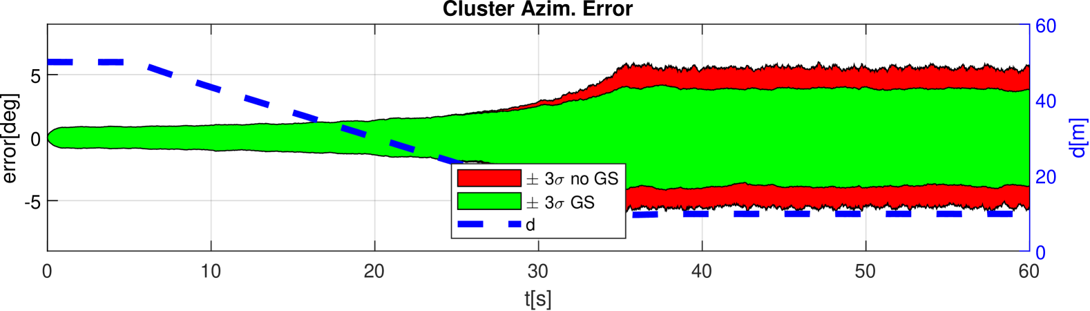
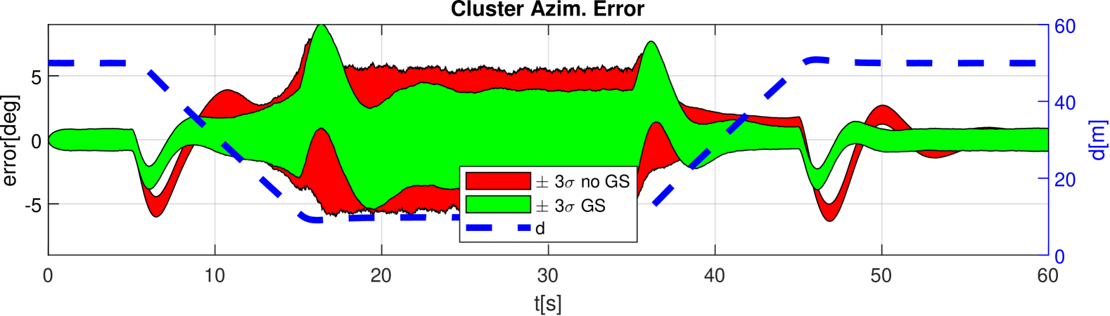
Figure 4: 2R formation statistic plot. Top: Azimuth in hovering. Bottom: Azimuth in tracking.

2R Obstacle avoidance maneuver

In Fig. 3 (right), an obstacle avoidance maneuver is proposed. The idea behind this maneuver is to pose a challenge on the controllers. The formation has to turn while shrinking, then pass between the obstacles and finally turn again while expanding and moving towards its final position.

In this simulation, the turning while shrinking maneuver part takes place between t=5s and t=15s. In Fig. 4 (bottom), notice the difference in the transient behaviors when the turning starts at t=5s and when it ends at t=15s. At t=5s the higher BW of the adaptive controller renders an improved transient, while at t=15s it renders an improved response to noise with a lower BW feedback controller. Also notice during the obstacles traversing part from t=20s to t=35s, the adaptive controller shows improved $\pm 3\sigma$ bounds.

5.2 Three Robot System (3R)

 

Figure 5: Variable geometries emphasizing characteristics for: roll/yaw GS (left) and pitch GS (right).

In the case of the 3R cluster, six different scenarios where simulated, three of them in hovering, and three other performing maneuvers. All simulations were carried out with geometry transitions which are described in Fig. 5.

To show the improved characteristics of the adaptive controller, simulated noise was injected on the position measurements of each individual robot in the same way as for the 2R case. For all scenarios, comparisons were carried out between an adaptive controller and another one with constant gains. The integral $K_{\omega}^{i}$ and proportional $K_{\omega}^{p}$ gains for the former were given by:

$$K_{\omega}^{i} =diag(k_{\omega_{x}}^{i}(\lambda_{x}),k_{\omega_{y}}^{i}(\lambda_{y}),k_{\omega_{z}}^{i}(\lambda_{z})),$$ (17)

$$K_{\omega}^{p} =diag(k_{\omega_{x}}^{p}(\lambda_{x}),k_{\omega_{y}}^{p}(\lambda_{y}),k_{\omega_{z}}^{p}(\lambda_{z})).$$ (18)

The $\lambda_{x,y,z}$ parameters are in the one dimensional unit simplex with

$$\lambda_{x,y,z}={\left(\sqrt{I_{{}_{x,y,z}}}-\sqrt{I_{x,y,z}^{min}}\right)}/{\left(\sqrt{I_{x,y,z}^{max}}-\sqrt{I_{x,y,z}^{min}}\right)}.$$ (19)

The computation of the gains is performed as:

$$k_{\omega_{x,y,z}}^{i}(\lambda) =k^{i_{1}}_{\omega_{x,y,z}}\left(1-\lambda_{x,y,z}\right)+k^{i_{2}}_{\omega_{x,y,z}}\lambda_{x,y,z},$$ (20)

$$k_{\omega_{x,y,z}}^{p}(\lambda) =k^{p_{1}}_{\omega_{x,y,z}}\left(1-\lambda_{x,y,z}\right)+k^{p_{2}}_{\omega_{x,y,z}}\lambda_{x,y,z}.$$ (21)

For all axes, $k_{\omega_{x,y,z}}^{p}(\lambda)={k_{\omega_{x,y,z}}^{i}(\lambda)}/{2}$, with the designed integral gains given as follows: $k^{i_{1}}_{\omega_{x}}=0.5$, $k^{i_{1}}_{\omega_{y}}=0.32$, $k^{i_{1}}_{\omega_{z}}=0.08$ $k^{i_{2}}_{\omega_{x}}=2.5$, $k^{i_{2}}_{\omega_{y}}=3.2$, $k^{i_{1}}_{\omega_{z}}=0.8$.

The rationale behind the proposed (19) GS strategy is as follows. In the 2R case, a simple small angles trigonometry argument allows for understanding that the constant power of measurement disturbances in robot space translates into a measurement disturbance in cluster space whose magnitude changes as the formation changes its geometry. Namely, in the 2R case, disturbance amplitudes are inversely proportional to the $d$ parameter. In the 2R case the $d$ parameter is proportional the square root of the formation’s inertia. Results confirm the main idea used for GS in this work which is: the higher the square root of the Inertia, the higher the attitude controllers’ gains. Extending this idea to the 3R case, GS takes place based upon the formula in Eq. (19).

In the examples shown below, $d_{2,3}^{max}=50m$ and $d_{2,3}^{min}=20m$. In turn, $\alpha_{max}=150^{\circ}$ and $\alpha_{min}=30^{\circ}$. These bounds on the geometry parameters allow for a minimum distance of $10m$ between robots 2 and 3, a lower bound compatible with the $\sigma=1m$ noise in a practical case.

The geometry transitions proposed for simulation in this work are shown in Fig. 5. They have the idea of going from high gains to low gains for all the axes of the cluster’s attitude controller. Because of the particular geometry of the 3R cluster, the geometry transition of Fig. 5 (left), renders a variation from maximum to minimum possible cluster inertia in the roll and yaw axes while the transition of Fig. 5 (right) renders a variation from maximum to minimum possible cluster inertia in the pitch axis. For comparing, a controller with fixed gains was simulated operating on a formation in parallel with the formation being controlled by the adaptive controller. The fixed gains of this controller were set to be an average of the gains of the adaptive controller.

3R Formations in hovering

For this scenario, a batch of 1000 simulations each one taking 180 seconds was completed with the geometry transition depicted in Fig. 5 (left). The trajectory prescribed for the cluster prescribes a fixed position and a fixed orientation while $\alpha$, $d_{2}$ and $d_{3}$ go all from maximum to minimum. As a result of this geometry transition, the $x$ axis $I_{x}$ moment of inertia goes from maximum to minimum the transition taking place between t=40s to t=70s (see the dashed blue line of the $\sqrt{I_{rel}^{x}}$ parameter in Fig. 6 (top). The dimensionless $\sqrt{I_{rel}^{x}}$ represents a quantity related the $\lambda_{x}$ GS parameter of the controller. When $\sqrt{I_{rel}^{x}}$ is at its minimum $\lambda_{x}=0$ (lowest gain of the attitude controller). On the opposite, when $\sqrt{I_{rel}^{x}}$ is at its maximum $\lambda_{x}=1$ (higest gain of the attitude controller).

Fig. 6 (top) shows the 3 standard deviation ($3\sigma$) estimation for the roll angle tracking error (for simulations with a zero angle reference). An estimation of the statistic is carried out based upon 1000 runs, showing in green that in the case where the formation is spread (number “1” in Fig. 5 left), the adaptive controller is more sensitive to noise (red is covered by green) yet showing an acceptable $\pm 3\sigma$. When the formation ends its transition at t=70s, the adaptive controller (green) employing lower gains, shows an improved response with respect to the fixed gains controller (colored in red on the background of the plot). Similar responses can be seen for the pitch controller the transition being shown in Fig. 5 (right) and the statistics estimation being shown in Fig. 6 (middle). For the yaw axis, Fig. 6 (bottom) shows the comparison between the adaptive controller and the constant gains controller. With respect to the response to measurement noise, the improvement of the adaptive controller is not remarkable when doing GS with the gains being based upon variations on the $I_{zz}$ moment of inertia of the formation. This is due to the influence of the cross moments of inertia on the magnitude of the yaw angle estimation noise. However, as it will be seen in the next subsection, the adaptation strategy based upon the $\sqrt{I_{zz}}$ pays for the yaw controller, considerably pays off as tracking performance is concerned with a marginal benefit in the response to noise when completely shrinking formation geometry.

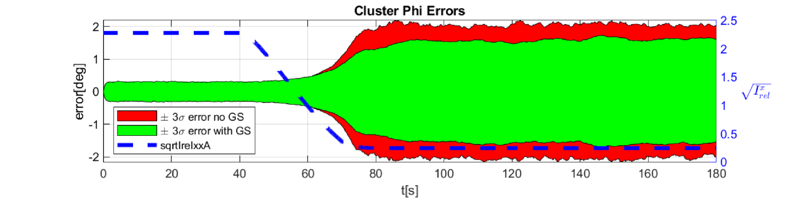
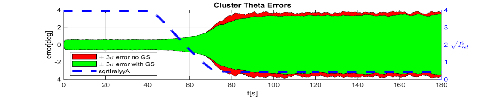
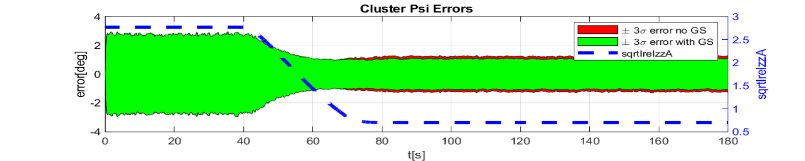
Figure 6: 3R Hovering, roll, pitch & yaw with geometry transitions.

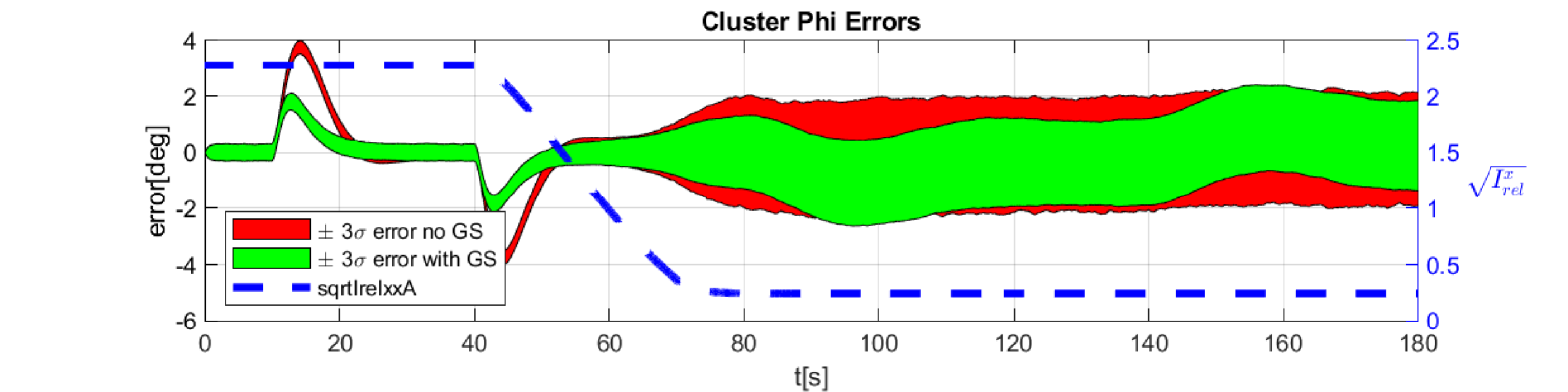
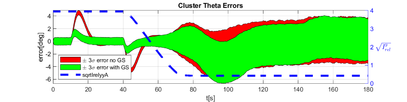
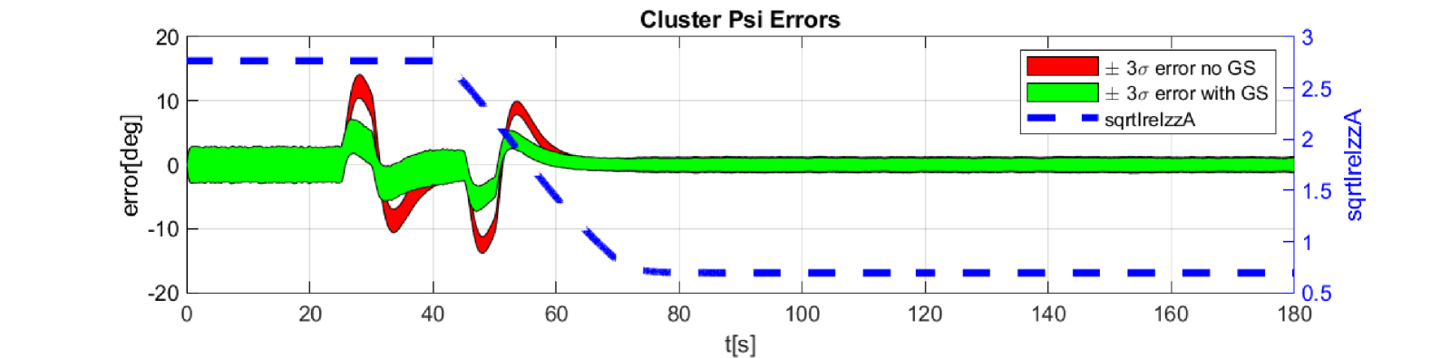
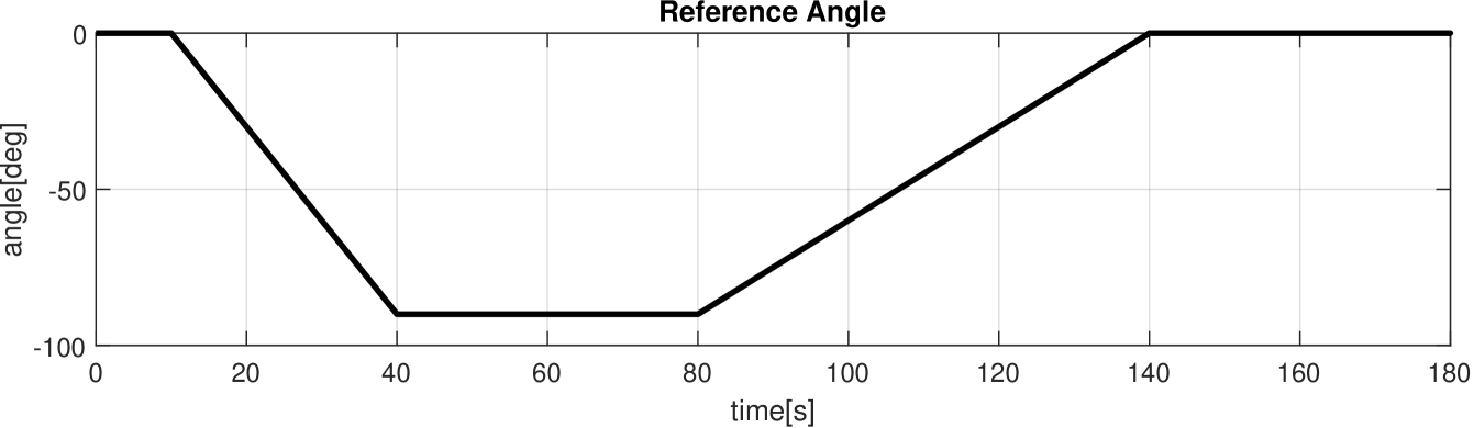
Figure 7: 3R roll, pitch & yaw maneuvers with geometry transitions. At the bottom, the commanded angle profile for all maneuvers.

3R Attitude Maneuvers

Some of the advantages of the adaptive controller become more evident when commanding formation maneuvers. The geometry transitions of Fig. 5 are here repeated, adding formation rotation commands in roll, pitch and yaw (one axis for each batch of simulations) as shown in Fig. 7 (bottom plot). Note in this plot, that a maneuver with a steeper slope is commanded firstly from t=10s to t=40s (30s rotation), since simulations start with geometries rendering maximum moment of inertia in the axis of interest a situation more favorable with respect to measurement noise. The 60s counter rotation starting at t=80s is commanded in a softer way given the less favorable geometry with respect to measurement noise where the feedback control strategy has been one where BW is lower when using the adaptive controller.

Note in Fig. 7 (first plot), the way the cloud of roll maneuvers while using the adaptive controller (in green), shows an improved average transient behavior while the acceptable noise rejection is slightly better for the red cloud (controller with constant lower gains). When the formation transitions to a geometry of lower gains and higher noise, the reference signal from 80s to 140s with a softer slope, helps the adaptive controller keep the error within acceptable bounds while showing a better response to noise. The same can be seen in Fig. 7 (second plot) for a pitch maneuver. As Fig. 7 (third plot) is concerned, for yaw, the performance improvement of the adaptive controller with respect to the constant gains controller must be pointed out. Note the response to noise during the first 25s of the statistical time analysis, shows that a more complex adaptation scheme could be tried to improve the response of the adaptive controller to noise. However a quick trade-off consideration suggests that the improvements with respect to transient performance are good enough to hold on to the proposed adaptation rule.

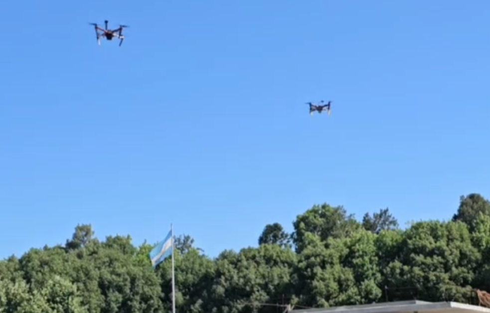
Figure 8: The UAVs used for experimental testing.

6 EXPERIMENTAL VALIDATION

In this section, experimental results of the proposed controller are presented. Specifically, results are shown for the case of two UAVs, where the previously described strategy based on the partial dual quaternion representation is applied.

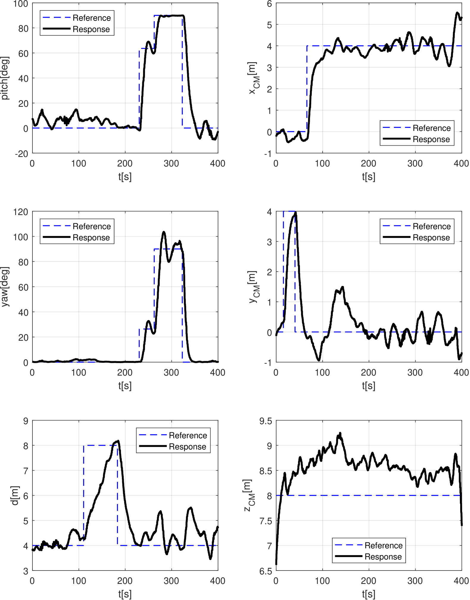
Figure 9: 2R cluster control experimental results.

The experiments were carried out using two F450 quadcopters, each equipped with a Pixhawk 4 flight controller running the PX4 firmware. These drones are powered by 3S LiPo batteries and use four brushless motors with 10-inch propellers. Each vehicle is fitted with a GPS module, altimeter, magnetometer and an IMU to estimate its position and orientation. The drones communicate with a ground computer via a wireless telemetry link. The ground computer receives navigation data from the drones, running the control algorithm and sending velocity commands back to the vehicles at a frequency of 10Hz.

In this work, dual quaternion operations and algorithms were implemented independently. However, leveraging libraries like DQ Robotics [1], which provides efficient and well-tested tools for robot modeling and control, could accelerate development and improve robustness. Future work will explore integrating such libraries and implementing the system within the Robot Operating System (ROS) framework [12] to enhance scalability and modularity.

Several flights were conducted, varying the position of the formation’s center of mass, its orientation, and the formation geometry, including the distance between the vehicles. These variations allowed for testing the controller under different configurations and scenarios.

Fig. 8 shows the experimental setup used in the tests. Each UAV, with an inner control system, is capable of maintaining its position within an error of 1.5 meters when zero velocity is commanded. Fig. 9 (first and second curves) presents the orientation of the cluster in terms of the pitch and yaw angles of the formation, demonstrating how the vehicles maintain stability and coordination. Fig.  9 (third curve) illustrates how the distance between the vehicles in the formation is tracked, ensuring that the separation remains constant throughout the flight. Finally, Fig. 9 (bottom curve) shows the tracking of the formation’s center, highlighting how the UAVs adjust their trajectories to keep the center of the formation within a predefined target.

7 CONCLUSION

In this work, a dual quaternion-based control strategy for multi-rotor UAV formation flight was presented, utilizing a virtual structure to coordinate small UAV groups. The approach simplifies formation control by abstracting individual UAV behavior, enabling intuitive management of pose and geometry. The method is effective for applications like cooperative cargo transport and aerial filming, where precise synchronization is essential.

Simulations results and experimental tests validated the strategy’s robustness under varying conditions, showing its ability to maintain stability while coping with disturbances and dynamic mission parameters. A key contribution is the treatment of shape variables as parameters rather than control objectives, enhancing flexibility while reducing control complexity.

Challenges remain, such as singularities in certain configurations, which future research could address to improve adaptability to diverse formations. Overall, this study underscores the potential of dual quaternion-based control for advancing multi-UAV systems, with promising applications in a wide range of real-world use cases.

References

- [1] B. V. Adorno and M. M. Marinho. DQ Robotics: A Library for Robot Modeling and Control. IEEE Robotics and Automation Magazine, 28:102–116, 2021.
- [2] W. K. Clifford. A preliminary sketch of biquaternions. Macmillan and Co., 1873.
- [3] Hai T. Do, Hoang T. Hua, Minh T. Nguyen, Cuong V. Nguyen, Hoa TT. Nguyen, Hoa T. Nguyen, and Nga TT. Nguyen. Formation control algorithms for multiple-uavs: A comprehensive survey. EAI Endorsed Transactions on Industrial Networks and Intelligent Systems, 8(27), 6 2021.
- [4] João Gutemberg Farias, Edson De Pieri, and Daniel Martins. A review on the applications of dual quaternions. Machines, 12(6), 2024.
- [5] J. I. Giribet, L. J. Colombo, P. Moreno, I. Mas, and D. Dimarogonas. Dual quaternion cluster-space formation control. IEEE Robotics and Automation Letters, 6(4):6789–6796, 2021.
- [6] Yan Jiang, Tingting Bai, and Yin Wang. Formation control algorithm of multi-UAVs based on alliance. Drones, 6(12), 2022.
- [7] Jing Li. Relative position and attitude coordinated control based on unit dual quaternion. Advances in Mechanical Engineering, 10(12), 2018.
- [8] H. Marciano, D. Dourado Villa, M. Sarcinelli-Filho, and J. I. Giribet. Dual quaternion-based control for a leader-follower formation of two quadrotors. In 2024 International Conference on Unmanned Aircraft Systems (ICUAS), pages 732–739, 2024.
- [9] I. Mas and C. Kitts. Quaternions and dual quaternions: Singularity-free multirobot formation control. Journal of Intelligent & Robotic Systems, 87:643–660, 2017.
- [10] I. Mas and C. A. Kitts. Dynamic control of mobile multirobot systems: The cluster space formulation. IEEE Access, 2:558–570, 2014.
- [11] Liqun Qi, Chunfeng Cui, and Chen Ouyang. Unit dual quaternion directed graphs, formation control and general weighted directed graphs. arXiv preprint, arXiv:2401.05132v6, Nov 2024.
- [12] Kaibiao Yang, Wenhan Dong, Yingyi Tong, and Lei He. Leader-follower formation consensus of quadrotor UAVs based on prescribed performance adaptive constrained backstepping control. Internationa Journal of Control Automation Systems, 20(12):3138–3154, 2022.
- [13] Yuxia Yuan and Markus Ryll. Dual quaternion control of uavs with cable-suspended load. 2024 IEEE International Conference on Robotics and Automation (ICRA), pages 1561–1567, 2024.