Hands-Off Covariance Steering: Inducing Feedback Sparsity via Iteratively Reweighted $\ell_{1,p}$ Regularization

Abstract

We consider the problem of optimally steering the state covariance matrix of a discrete-time linear stochastic system to a desired terminal covariance matrix, while inducing the control input to be zero over many time intervals. We propose to induce sparsity in the feedback gain matrices by using a sum-of-norms version of the iteratively reweighted $\ell_{1}$-norm minimization. We show that the lossless convexification property holds even with the regularization term. Numerical simulations show that the proposed method produces a Pareto front of transient cost and sparsity that is not achievable by a simple $\ell_{1}$-norm minimization and closely approximates the $\ell_{0}$-norm minimization obtained from brute-force search.

I Introduction

Sparsity is important for the control and identification of systems. It is often represented by the $\ell_{0}$-(pseudo) norm, which is the number of nonzero elements in a vector. For example, a sparse signal recovery problem can be posed as

$$\min_{x}\ \|x\|_{0}\quad\text{s.t.}\quad y=Ax$$ (1)

where $x$ is the signal to be recovered, $y$ is the noisy measurement, and $A$ is the measurement matrix. Unfortunately, the $\ell_{0}$-norm is non-convex and nondifferentiable, and 1 is NP-hard [1]. On the other hand, the $\ell_{1}$-norm is convex and differentiable, and its sparsity-inducing property has been demonstrated in various applications [2, 3, 4, 5]. In system identification, perhaps the most well-known algorithm for inducing sparsity is the LASSO algorithm [2]. Compared to ordinary least squares, the LASSO algorithm adds a constraint on the $\ell_{1}$-norm of the parameter vector, which induces sparsity in the model selection. Basis Pursuit [3] uses the $\ell_{1}$-norm in the objective function for sparse signal recovery, solving the problem

$$\min_{x}\ \|x\|_{1}\quad\text{s.t.}\quad y=Ax$$ (2)

The applications of the $\ell_{1}$-norm regularization are vast, and we refer the reader to [4] for a comprehensive review.

Sparsity can be especially favorable in control of systems where every control input incurrs a large cost (e.g. financial/human) , such as in multi-period investment problems [6], economics [7], and on-ground computation of spacecraft trajectory correction maneuvers [8]. As pointed out in [9], an optimal control problem with sparsity consideration can be considered as a multi-objective optimization problem that trades control performance and control input sparsity. Ref. [10] solves an $\ell_{1}$-norm minimization problem to design sparse feedback gains, i.e. only a few sensor-to-actuator paths are used for feedback control. Ref. [11] solves a sum-of-norms regularization problem to track waypoints while also regularizing the sum-of-norms of the impulse train which constitute the input signal. Sum-of-norms regularization is a generalization of the $\ell_{1}$-norm regularization, where the parameter vector is divided into groups, and the sum of the $p$-norms of the groups is minimized, promoting group sparsity. Ref. [12] shows the equivalence between the sparsest control and $\ell_{1}$-optimal control. Recent works consider both the transient cost and sparsity, for example, for linear quadratic regulator (LQR) problems. Representative solution methods are the alternating direction method of multipliers (ADMM) [13], branch and bound [14], and $\ell_{1}$-norm regularization [15]. Some works refer to control problems with sparsity consideration as hands-off control, which gives the name hands-off covariance steering for our problem.

Covariance steering [16, 17, 18, 19, 20, 21] is a problem of finding the optimal feedback gain matrices that minimize the expected quadratic cost function, while steering the state covariance matrix to a desired terminal covariance matrix under linear noisy dynamics. Combined with control sparsity, hands-off covariance steering can control the state distribution to satisfy distributional/chance constraints while keeping the control input zero for many time intervals, relieving the implicit cost for implementing controls in real-world systems.

As the solution method, we return to the question posed by [4] for sparse signal recovery: “Can we improve upon $\ell_{1}$-norm minimization to better approximate $\ell_{0}$-norm minimization?” The influential work [4] proposes to solve the iteratively reweighted $\ell_{1}$-norm minimization (IRL1)

$$\min_{x}\ \sum_{i}w_{i}|x_{i}|\quad\text{s.t.}\quad y=Ax$$ (3)

with weights $w_{i}$ updated based on the solution of the previous iteration. The authors show that this recovers the original signal $x$ more accurately than the unweighted $\ell_{1}$-norm minimization. While a common approach in $\ell_{1}$-norm regularization is to tune the scalar regularization parameter to achieve the desired sparsity, we observed that for covariance steering, even extremely large regularization parameters failed to produce sufficiently sparse solutions.

Our main contributions are as follows:

• We propose a method to induce sparse control in the chance-constrained covariance steering problem by combining the iteratively reweighted $\ell_{1}$-norm minimization with sum-of-norms regularization.

• We show that the lossless convexification property holds with the sparsity-promoting regularization term, enabling efficient computation via solving a series of semidefinite programming problems.

Notation: $\norm{\cdot}_{0}$, $\norm{\cdot}_{1}$, $\norm{\cdot}_{2}$, $\norm{\cdot}_{F}$, $\tr(\cdot)$, $\mathbb{E}\left[\cdot\right]$, $\mathrm{Cov}[\cdot]$, $\mathbb{P}\left[\cdot\right]$, $\det(\cdot)$, $\lambda_{\max}(\cdot)$ denote the $\ell_{0}$, $\ell_{1}$, $\ell_{2}$, Frobenius norm, trace, expectation, covariance, probability, determinant, and maximum eigenvalue, respectively. $\mathbb{R},\mathbb{R}^{n},\mathbb{R}^{n\times m}$ denote real numbers, $n$-dimensional real-valued vectors, and $n\times m$ real-valued matrices, respectively. $\mathbb{S}_{+}^{n}$ ($\mathbb{S}_{++}^{n}$) denotes the set of $n\times n$ symmetric positive semidefinite (definite) matrices. $\mathbb{Z}_{a:b}$ denotes the set of integers from $a$ to $b$. The symbol $\succeq$ ($\succ$) denotes (strict) matrix inequality between symmetric matrices.

II Preliminaries

In this section, we provide a brief review of covariance steering, $\ell_{1}$-norm regularization, and its reweighted version.

II-A Covariance Steering

Covariance steering aims to design a feedback control policy that minimizes the expected cost function while steering the covariance matrix of the state to a desired terminal covariance matrix. Recently, both the continuous-time [19] and discrete-time [17, 18, 20] versions of the problem have been studied. Here, we consider the finite-horizon, discrete-time version with horizon $N$:

$$\min_{\pi} \quad J_{\Sigma}:=\mathbb{E}\left[\sum_{k=0}^{N-1}x_{k}^{\top}Q_{k}x_{k}+u_{k}^{\top}R_{k}u_{k}\right]$$ (4a)

s.t. $$x_{k+1}=A_{k}x_{k}+B_{k}u_{k}+D_{k}w_{k},\quad k\in\mathbb{Z}_{0:N-1}$$ (4b)

$$\mathbb{E}\left[x_{0}\right]=\mu_{0},\ \mathbb{E}\left[x_{N}\right]=\mu_{N}$$ (4c)

$$\mathrm{Cov}[x_{0}]=\bar{\Sigma}_{0},\ \mathrm{Cov}[x_{N}]\preceq\bar{\Sigma}_{N}$$ (4d)

$$u_{k}=\pi(x_{k},k),\quad k\in\mathbb{Z}_{0:N-1}$$ (4e)

where $x_{k}\in\mathbb{R}^{n}$, $u_{k}\in\mathbb{R}^{m}$ are the state and control input at time $k$, respectively. $w_{k}\in\mathbb{R}^{p}$ is a white, zero-mean, Gaussian noise with identity covariance matrix. $A_{k}\in\mathbb{R}^{n\times n}$, $B_{k}\in\mathbb{R}^{n\times m}$, $D_{k}\in\mathbb{R}^{n\times p}$ are the system matrices. $Q_{k}\in\mathbb{S}_{+}^{n}$, $R_{k}\in\mathbb{S}_{++}^{n}$ are the state and control input cost matrices. $\mu_{0}\in\mathbb{R}^{n}$, $\mu_{N}\in\mathbb{R}^{n}$ are the initial and terminal state mean vectors. $\bar{\Sigma}_{0}\in\mathbb{S}_{++}^{n}$, $\bar{\Sigma}_{N}\in\mathbb{S}_{++}^{n}$ are the initial and terminal covariance matrices, with $\bar{\Sigma}_{N}\succ D_{N-1}D_{N-1}^{\top}$.

Assumption 1.

$A_{k}$ is invertible for $k\in\mathbb{Z}_{0:N-1}$.

This assumption is reasonable, since the state transition matrix of a continuous-time dynamical system is invertible, and the discrete-time equation is obtained by discretization.

Assumption 2.

$\mathrm{Cov}[x_{k}]\succ 0$ for $k\in\mathbb{Z}_{0:N}$.

This assumption is also reasonable, as most real-life problems involve nondegenerate covariance matrices.

Assumption 3.

$\mu_{0}=\mu_{N}=0$, $\mathbb{E}\left[x_{k}\right]=0$ for $k\in\mathbb{Z}_{0:N}$

This assumption is made for simplicity and allows us to focus on the covariance dynamics in this paper.

We consider an affine feedback policy, which has been shown to be optimal [17, 20] in the unconstrained covariance steering setting:

$$u_{k}=K_{k}x_{k}$$ (5)

where $K_{k}$ is the feedback gain matrix. From standard derivations, the covariance propagation equation is given by

$$\Sigma_{k+1} =(A_{k}+B_{k}K_{k})\Sigma_{k}(A_{k}+B_{k}K_{k})^{\top}+D_{k}D_{k}^{\top}$$ (6)

and the objective function by

$$J_{\Sigma}=\sum_{k=0}^{N-1}\tr(Q_{k}\Sigma_{k})+\tr(R_{k}K_{k}\Sigma_{k}K_{k}^{\top})$$ (7)

Then, 4 is cast as a parameter optimization problem:

$$\min_{K_{k},\Sigma_{k}}\ \lx@cref{creftype~refnum}{eq:cost_function_in_K}\quad\text{s.t.}\ \lx@cref{creftype~refnum}{eq:covariance_propagation_in_K},\ \Sigma_{0}=\bar{\Sigma}_{0},\ \Sigma_{N}\preceq\bar{\Sigma}_{N}$$ (8)

Note that both the feedback gains $K_{k}$ and the covariance matrices $\Sigma_{k}$ are optimization variables, making 8 nonconvex due to the equality constraint 6. However, through a process called lossless convexification, the solution to 8 can be obtained by solving a convex optimization problem [20]. Here, we review the solution method proposed in [20]. We begin by performing a change of variables by defining

$$U_{k}:=K_{k}\Sigma_{k}$$ (9)

Note that $K_{k}$ can be recovered uniquely from $U_{k}$ as $K_{k}=U_{k}\Sigma_{k}^{-1}$ from Assumption 2. With this change of variables, 6 and 7 are respectively rewritten as

$$\Sigma_{k+1} =A_{k}\Sigma_{k}A_{k}^{\top}+A_{k}U_{k}^{\top}B_{k}^{\top}+$$

$$\quad B_{k}U_{k}A_{k}^{\top}+B_{k}U_{k}\Sigma_{k}^{-1}U_{k}^{\top}B_{k}^{\top}+D_{k}D_{k}^{\top}$$ (10)

$$J_{\Sigma} =\sum_{k=0}^{N-1}\tr(Q_{k}\Sigma_{k})+\tr(R_{k}U_{k}\Sigma_{k}^{-1}U_{k}^{\top})$$ (11)

Next, introduce variables

$$Y_{k}:=U_{k}\Sigma_{k}^{-1}U_{k}^{\top}(=K_{k}\Sigma_{k}K_{k}^{\top})$$ (12)

and replace the relevant expressions in Sections II-A and 11. While 12 is nonconvex, it can be relaxed to a matrix inequality as

$$Y_{k}\succeq U_{k}\Sigma_{k}^{-1}U_{k}^{\top}$$ (13)

which, from Schur’s Lemma, is equivalent to the linear matrix inequality

$$\begin{bmatrix}\Sigma_{k}&U_{k}^{\top}\\ U_{k}&Y_{k}\end{bmatrix}\succeq 0$$ (14)

8 now takes the form of a semidefinite programming (SDP):

$$\min_{\Sigma_{k},U_{k},Y_{k}}\ J_{\Sigma}=\sum_{k=0}^{N-1}\tr(Q_{k}\Sigma_{k})+\tr(R_{k}Y_{k})$$ (15a)

$$\quad\text{s.t.}\quad\Sigma_{0}=\bar{\Sigma}_{0},\quad\Sigma_{N}\preceq\bar{\Sigma}_{N}$$ (15b)

$$\Sigma_{k+1}=A_{k}\Sigma_{k}A_{k}^{\top}+A_{k}U_{k}^{\top}B_{k}^{\top}+B_{k}U_{k}A_{k}^{\top}$$

$$\quad+B_{k}Y_{k}B_{k}^{\top}+D_{k}D_{k}^{\top},\quad k\in\mathbb{Z}_{0:N-1}$$ (15c)

$$\begin{bmatrix}\Sigma_{k}&U_{k}^{\top}\\ U_{k}&Y_{k}\end{bmatrix}\succeq 0,\quad k\in\mathbb{Z}_{0:N-1}$$ (15d)

[20] shows that the solution obtained from solving this convex problem (after changing back the variables to $K_{k}$) is equivalent to the solution obtained from the original nonconvex problem 8. Since the equality 12 is satisfied at the optimal solution of 15, $Y_{k}$ will be equivalent to the covariance matrix of the input $u_{k}$.

II-B Group Sparsity via Sum-of-Norms Regularization

While $\ell_{1}$ regularization is useful for inducing element-wise sparsity, it cannot be directly applied to induce sparsity in groups of elements [22]. In this case, the regularization term takes the general sum-of-norms form [23]

$$\sum_{g\in G}\|x_{g}\|_{p}$$ (16)

Here, $G$ is a set of groups, and $x_{g}$ is the vector of features in group $g$. This regularization promotes sparsity in the groups, i.e. it encourages the use of only a few groups. Naturally, this is also called the $\ell_{1,p}$-norm and can be thought of as a generalization of the $\ell_{1}$-norm. There are several choices for $p$; $p=2$ is standard in group LASSO [23], $p=\infty$ is also sparsity-inducing. However, $p=1$ does not promote group sparsity [22].

II-C Iteratively Reweighted $\ell_{1}$ Minimization

Although the $\ell_{1}$-norm regularization is widely used for inducing sparsity, its solution can be suboptimal in terms of sparsity. In the context of signal processing, [4] proposes IRL1 to better approximate the $\ell_{0}$-norm minimization, as in 3. By iteratively solving the weighted $\ell_{1}$-norm minimization problem with weights updated based on the solution of the previous iteration, [4] shows that the solution recovers the original signal $x$ accurately. The weight update rule is given by

$$w_{i}^{(l+1)}=\frac{1}{|x_{i}^{(l)}|+\epsilon},\quad w_{i}^{(1)}=1$$ (17)

where $l$ is the iteration index, and $\epsilon$ is a small positive constant, used to avoid division by zero. Intuitively, the weights are updated such that for elements of $x$ that are close to zero in the previous iteration, the weights are large, promoting sparsity in the subsequent solution. 17 is the first-order term in the linearization of the (nonconvex) penalty function [4]

$$\phi_{\log,\epsilon}(t)=\log(1+|t|/\epsilon)$$ (18)

for $t=x_{i}^{(l)}$, which, when multipled by a constant $c=1/\phi_{\log,\epsilon}(1)$, approaches the discontinuous penalty function

$$\phi_{0}(t)=\begin{cases}1&t\neq 0\\ 0&t=0\end{cases}$$ (19)

as $\epsilon\rightarrow 0$. See Fig. 1 for a visualization.

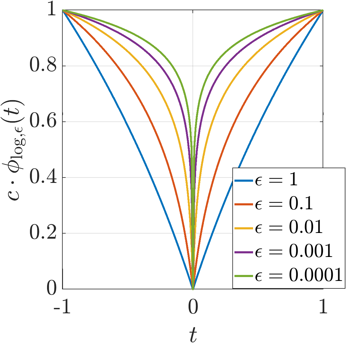
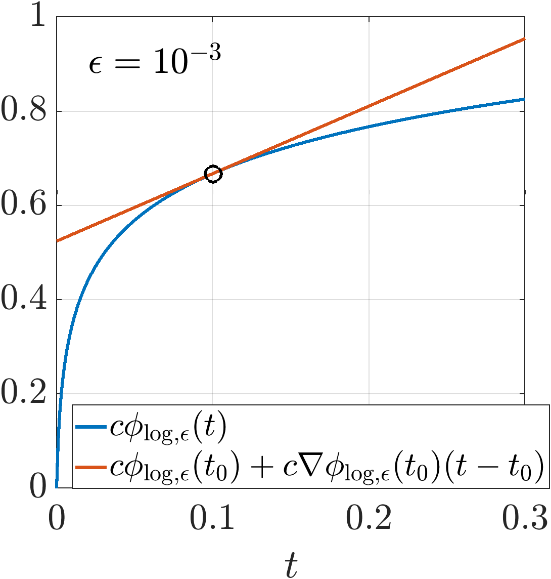
Figure 1: Left: $\phi_{\log,\epsilon}(t)$ approaches $\phi_{0}(t)$ as $\epsilon\rightarrow 0$. Right: For $t_{0}>0$, $\nabla\phi_{\log,\epsilon}(t_{0})=1/(t_{0}+\epsilon)$, which gives the weighted $\ell_{1}$ penalty, with its gradient becoming steeper as $t_{0}\rightarrow 0$.

III Hands-Off Covariance Steering

III-A Problem Formulation

Define a binary vector $\tau\in\{0,1\}^{N}$, where $\tau_{k}$ is such that

$$\tau_{k}=\begin{cases}1&\text{if }\mathbb{P}\left[u_{k}=0\right]=1\\ 0&\text{otherwise}\end{cases}$$ (20)

Hands-off covariance steering is a multi-objective optimization problem that trades off the transient cost and the sparsity of the feedback gains as follows:

$$\min_{\pi,\tau}\quad[J_{\Sigma},\ J_{\tau}:=\sum_{k=0}^{N-1}\tau_{k}]\quad\text{s.t.}\ \lx@cref{creftype~refnum}{eq:covariance_propagation_in_K},\lx@cref{creftype~refnum}{eq:boundary_conditions},\lx@cref{creftype~refnum}{eq:tau_definition}$$ (21)

Our objective is to find, in a computationally tractable manner, an approximate Pareto front of the transient cost and sparsity.

When our control policy takes the form 5, we want the feedback gain matrices $(K_{k})_{k=0}^{N-1}$ to be zero for many time intervals. Since the feedback gains are related to the variables $(Y_{k})_{k=0}^{N-1}$ through the relation 13, we place a regularization term on $(Y_{k})_{k=0}^{N-1}$. We will show later that $Y_{k}=0$ if and only if $K_{k}=0$ from Assumption 2.

III-B Regularized Covariance Steering

A natural first step to solve 21 is to add a regularization term to the objective function and to vary the regularization parameter. The regularized covariance steering problem is given by

$$\min_{\Sigma_{k},U_{k},Y_{k}}J_{\Sigma}+\lambda\sum_{k=0}^{N-1}\|Y_{k}\|_{F}\text{ s.t. }\lx@cref{creftype~refnum}{eq:boundary_conditions_2},\lx@cref{creftype~refnum}{eq:covariance_dynamics_in_Y},\lx@cref{creftype~refnum}{eq:psd_constraint}$$ (22)

where $\lambda>0$ is the regularization parameter. Note that taking the Frobenius norm of $Y_{k}$ is equivalent to taking the $\ell_{2}$-norm of the vectorized form of $Y_{k}$. Hence, this is a $\ell_{1,2}$ norm-regularized covariance steering problem.

However, as we demonstrate in Section IV, solving the problem with this objective function does not always provide sparsity in the feedback gains. As a method of inducing sparsity, we turn to the IRL1 method.

III-C IRL1P for Covariance Steering

Sum-of-norms regularization and IRL1 are combined here as a way of achieving better sparsity in the solution. We call this method the iteratively reweighted $\ell_{1,p}$-norm minimization (IRL1P). The problem is given by

$$\hskip-3.0pt\min_{\Sigma_{k},U_{k},Y_{k}}J_{\Sigma}+\lambda\sum_{k=0}^{N-1}w_{k}^{(l)}\|Y_{k}\|_{F}\ \text{ s.t. }\lx@cref{creftype~refnum}{eq:boundary_conditions_2},\lx@cref{creftype~refnum}{eq:covariance_dynamics_in_Y},\lx@cref{creftype~refnum}{eq:psd_constraint}$$ (23)

The update rule for the weights is given by

$$w_{k}^{(l+1)}=\frac{1}{\|Y_{k}^{(l)}\|_{F}+\epsilon},\quad w_{k}^{(1)}=1,\ k\in\mathbb{Z}_{0:N-1}$$ (24)

and the algorithm terminates when

$$\frac{\sum_{k=0}^{N-1}(\norm{K_{k}}_{F}^{(l)}-\norm{K_{k}}_{F}^{(l-1)})}{\sum_{k=0}^{N-1}\norm{K_{k}}_{F}^{(l-1)}}<\epsilon_{\mathrm{conv}}$$ (25)

for some tolerance $\epsilon_{\mathrm{conv}}>0$. For completeness, the pseudocode is given in Algorithm 1.

$\lambda,\epsilon,\epsilon_{\mathrm{conv}},l_{\max}$

1:Initialize $w_{k}^{(1)}=1,\ k\in\mathbb{Z}_{0:N-1}$ $l<l_{\max}$

2:Solve 23 with $\lambda,w_{k}^{(l)}$

3:Retrieve feedback gains $K_{k}=U_{k}\Sigma_{k}^{-1},\ k\in\mathbb{Z}_{0:N-1}$

4:If $l>1$ and 25 are satisfied, break

5:Update weights $w_{k}^{(l+1)}=\frac{1}{\|Y_{k}^{(l)}\|_{F}+\epsilon},\ k\in\mathbb{Z}_{0:N-1}$

6:$l\leftarrow l+1$

7:return $K_{k},Y_{k}$ for $k\in\mathbb{Z}_{0:N-1}$, $\Sigma_{k}$ for $k\in\mathbb{Z}_{0:N}$

Algorithm 1 Iteratively Reweighted $\ell_{1,p}$-norm Minimization for Covariance Steering

Remark 1.

The original IRL1 paper [4] provides no guarantee of convergence. A related work [24] shows that for problems of the form

$$\min_{x}\norm{Ax-b}_{2}^{2}+\lambda\norm{x}_{p}^{p},\quad 0<p<1$$ (26)

replacing the regularization term with the weighted $\ell_{1}$-norm and applying the IRL1 procedure produces a bounded sequence and any accumulation point is a stationary point of 26. At this point, we do not provide a convergence proof for Algorithm 1. However, as has been demonstrated in many other applications, the method is effective in both convergence and providing a sparse solution.

Assumption 4.

Slater’s condition holds for 23, i.e. there exists a strictly feasible solution for 23.

III-D Addition of Chance Constraints

In addition to the standard formulation in 21, we consider chance constraints on the control input’s Euclidean norm:

$$\mathbb{P}\left[\norm{u_{k}}_{2}\leq u_{\max}\right]\geq 1-\gamma$$ (27)

where $0<\gamma<1$ is a user-specified probability of violating the term inside $\mathbb{P}\left[\cdot\right]$. The following lemma enables us to tractably reformulate 27 in a deterministic parameter optimization:

Lemma 1 (Lemma 3, [8]).

For a Gaussian random vector $\xi\in\mathbb{R}^{n}$ with mean $\mu$ and covariance matrix $\Sigma$, the quantile function of $\norm{\xi}_{2}$, denoted by $\mathcal{Q}_{\norm{\xi}_{2}}(p)$, is upper bounded as

$$\mathcal{Q}_{\norm{\xi}_{2}}(p)\leq\norm{\mu}_{2}+\sqrt{\mathcal{Q}_{\chi_{n}^{2}}(p)\lambda_{\max}(\Sigma)}$$ (28)

where $\mathcal{Q}_{\chi_{n}^{2}}(p)$ is the $p$-quantile of the $\chi^{2}$ distribution with $n$ degrees of freedom.

From Lemma 1, 27 can be imposed as

$$\mathbb{E}\left[u_{k}\right]+\sqrt{\mathcal{Q}_{\chi_{m}^{2}}(1-\gamma)\lambda_{\max}(\mathrm{Cov}[u_{k}])}\leq u_{\max}$$ (29)

From Assumption 3, $\mathbb{E}\left[u_{k}\right]=0$ for $k\in\mathbb{Z}_{0:N-1}$. Moving terms around,

$$\lambda_{\max}(\mathrm{Cov}[u_{k}])\leq\frac{u_{\max}^{2}}{\mathcal{Q}_{\chi_{n}^{2}}(1-\gamma)}$$ (30)

Assuming that lossless convexification holds under chance constraints, i.e. $Y_{k}=\mathrm{Cov}[u_{k}]$, which we later prove in Theorem 1, 30 can be rewritten as

$$\lambda_{\max}(Y_{k})\leq\rho:=\frac{u_{\max}^{2}}{\mathcal{Q}_{\chi_{n}^{2}}(1-\gamma)}$$ (31)

which can be readily included in 23, still as an SDP [5].

Remark 2.

Chance constraints are not restricted to this form or to be on the control input; see e.g. [8] for other deterministic reformulations of chance constraints, such as hyperplane constraints.

III-E Lossless Convexification with Regularization

Here, we show that the lossless convexification property shown in [20] holds even with the regularization term in 23 and chance constraints in 31. Define $F_{k},G_{k},h_{k}$ as

$$F_{k} :=A_{k}\Sigma_{k}A_{k}^{\top}+A_{k}U_{k}^{\top}B_{k}^{\top}+B_{k}U_{k}A_{k}^{\top}$$

$$\quad+B_{k}Y_{k}B_{k}^{\top}+D_{k}D_{k}^{\top}-\Sigma_{k+1}$$ (32)

$$G_{k} :=U_{k}\Sigma_{k}^{-1}U_{k}^{\top}-Y_{k}$$ (33)

$$h_{k} :=\lambda_{\max}(Y_{k})-\rho$$ (34)

Eq. 23, without boundary conditions, is now written as

$$\min_{\Sigma_{k},U_{k},Y_{k}} \sum_{k=0}^{N-1}\tr(Q_{k}\Sigma_{k})+\tr(R_{k}Y_{k})+\lambda w_{k}\|Y_{k}\|_{F}$$ (35a)

s.t. $$F_{k}=0,\ G_{k}\preceq 0,\ h_{k}\leq 0$$ (35b)

The following lemma is used in the proof.

Lemma 2 (Lemma 1, [20]).

Let $A$ and $B$ be $n\times n$ symmetric matrices with $A\succeq 0$, $B\preceq 0$, and $\tr(AB)=0$. If $B$ has at least one nonzero eigenvalue, then $A$ is singular.

Theorem 1.

At the optimal solution of 23, $G_{k}=0$ for $k\in\mathbb{Z}_{0:N-1}$, hence the relaxation is lossless.

Proof.

Let $\Lambda_{k}$, $\Gamma_{k}$, $\eta_{k}$ be the Lagrange multipliers for $F_{k}$, $G_{k}$, $H_{k}$ respectively. $\Gamma_{k}$ is symmetric by definition, and $\Lambda_{k}$ is symmetric because of the symmetry in $F_{k}$. Assumption 4 (Slater’s condition) implies strong duality. Then, from strong duality, the Karush-Kuhn-Tucker (KKT) conditions are necessary (and sufficient) for optimality [5]. The Lagrangian is given by

$$\mathcal{L}(\Sigma_{k},U_{k},Y_{k},\Lambda_{k},\Gamma_{k})=\sum_{k=0}^{N-1}\tr(Q_{k}\Sigma_{k})+\tr(R_{k}Y_{k})$$

$$\quad+\lambda w_{k}\|Y_{k}\|_{F}+\tr(\Lambda_{k}F_{k})+\tr(\Gamma_{k}G_{k})+\eta_{k}h_{k}$$ (36)

The relevant KKT conditions are given by

$$\frac{\partial\mathcal{L}}{\partial U_{k}}=2\Gamma_{k}U_{k}\Sigma_{k}^{-1}+2B_{k}^{\top}\Lambda_{k}A_{k}=0$$ (37a)

$$\frac{\partial\mathcal{L}}{\partial Y_{k}}=R_{k}+\frac{\lambda w_{k}Y_{k}}{\|Y_{k}\|_{F}}-\Gamma_{k}+\eta_{k}v_{k}v_{k}^{\top}+B_{k}^{\top}\Lambda_{k}B_{k}=0$$ (37b)

$$F_{k}=0,\ G_{k}\preceq 0,\ H_{k}\leq 0\quad\text{(primary feasibility)}$$ (37c)

$$\Gamma_{k}\succeq 0,\eta_{k}\geq 0\quad\text{(dual feasibility)}$$ (37d)

$$\tr(\Gamma_{k}^{\top}G_{k})=\eta_{k}h_{k}=0\ \ \text{(complementary slackness)}$$ (37e)

where $v_{k}$ is the eigenvector corresponding to the largest eigenvalue of $Y_{k}$. From 37a, we have

$$B_{k}^{\top}\Lambda_{k}=-\Gamma_{k}U_{k}\Sigma_{k}^{-1}A_{k}^{-1}$$ (38)

Substituting into 37b, we have

$$R_{k}+\frac{\lambda w_{k}Y_{k}}{\|Y_{k}\|_{F}}-\Gamma_{k}+\eta_{k}v_{k}v_{k}^{\top}-\Gamma_{k}U_{k}\Sigma_{k}^{-1}A_{k}^{-1}B_{k}=0$$ (39)

Now, we are ready to show the theorem statement using proof by contradiction. Assume that $G_{k}$ has at least one nonzero eigenvalue. From $G_{k}\preceq 0$, symmetry of $\Gamma_{k}$, and $\tr(\Gamma_{k}^{\top}G_{k})=0$, applying Lemma 2 gives that $\Gamma_{k}$ is singular. Then, moving terms in 39 and taking the determinant of both sides,

$$\det(R_{k}+\frac{\lambda w_{k}Y_{k}}{\|Y_{k}\|_{F}}+\eta_{k}v_{k}v_{k}^{\top})$$

$$\quad=\det(\Gamma_{k})\det(I+\Gamma_{k}U_{k}\Sigma_{k}^{-1}A_{k}^{-1}B_{k})$$ (40)

The LHS is positive, since $R_{k}\succ 0,\lambda\geq 0,Y_{k}\succeq 0$ by assumption and $\eta_{k}\geq 0$ from 37d. However, since $\Gamma_{k}$ is singular, its determinant, and hence the RHS is zero. Thus, we have a contradiction. ∎

Remark 3.

From Assumption 2, $Y_{k}=K_{k}\Sigma_{k}K_{k}^{\top}=0$ implies $K_{k}=0$. Then, $K_{k}=0\iff Y_{k}=0$. With Theorem 1, this justifies the use of the regularization on $Y_{k}$ in 23.

IV Numerical Example

Here, we show the solution obtained from hands-off covariance steering. SDPs are solved using YALMIP [25] and MOSEK [26]. We use some problem parameters from [20]: for $k\in\mathbb{Z}_{0:N-1}$, $Q_{k}=0.5I_{2}$, $R_{k}=1$,

$$A_{k}=\begin{bmatrix}1&0.2\\ 0&1\end{bmatrix},\ B_{k}=\begin{bmatrix}0.02\\ 0.2\end{bmatrix},\ D_{k}=\begin{bmatrix}0.4&0\\ 0.4&0.6\end{bmatrix}$$

We set the boundary covariance matrices as

$$\bar{\Sigma}_{0}=\begin{bmatrix}5&-1\\ -1&1\end{bmatrix},\quad\bar{\Sigma}_{N}=\begin{bmatrix}0.5&-0.4\\ -0.4&2\end{bmatrix}$$

The chance constraint is defined by $u_{\max}=10$, $\gamma=0.03$. We also note that for every problem solved, the lossless convexification was verified to hold (to some numerical tolerance).

IV-A Comparison with Brute-Force Search

To first demonstrate the capability of the IRL1P method to find a sparse solution that closely matches the global optimum, we compare the solution obtained from the method with the solution obtained from a brute-force search. The brute-force search is performed by solving $2^{N}$ convex optimization problems, where each problem imposes $Y_{k}=0$ for a set of nodes $k$. The solution with the smallest objective function value is chosen. To keep the search space small, we consider the problem with $N=8$. Furthermore, to emphasize the effectiveness for a wide range of sparsity, we exclude the chance constraints from the problem.

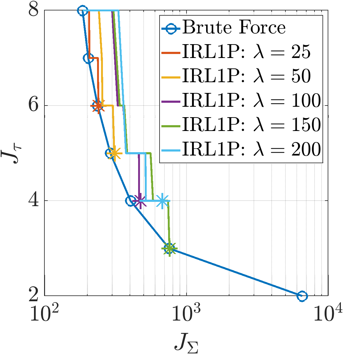
Figure 2: Comparison with brute-force search Pareto front. $*$ shows the final solution from IRL1P.

Fig. 2 shows the comparison. Overall, increasing $\lambda$ leads to a more sparse solution, i.e. smaller $J_{\tau}$. The final solution shows convergence to a pair $(J_{\Sigma},J_{\tau})$ that is close to the Pareto front obtained from the brute-force search. For example, using $\lambda=25$ converges to a solution with $J_{\tau}=6$ that is close to brute-force. The same can be said for $\lambda=50$ to $J_{\tau}=5$, $\lambda=100$ to $J_{\tau}=4$, and $\lambda=150$ to $J_{\tau}=3$. However, the solution from IRL1P fails to find a solution with the desired sparsity for $J_{\tau}=2$, most likely because this solution requires a large transient cost, and as a result many iterations. Nevertheless, the solution from IRL1P finds a near-optimal solution with a much smaller computational cost, and its effectiveness scales to problems with larger $N$. Brute-force search is not feasible for larger $N$ due to the exponential growth of the search space, while the computational complexity of IRL1P is proportional to the computational complexity of solving the SDP. The computational effort of the SDP has been demonstrated to grow approximately linearly with $N$ up to problem sizes of $N$ in the hundreds [27]. Cases where $J_{\tau}<2$ were infeasible for this problem setting. Since throughout the iteration progress, the solution from IRL1P is close to the Pareto front, this also suggests that the user can also choose to terminate the algorithm when the desired sparsity is achieved, if they are to accept some suboptimality.

IV-B Standard Covariance Steering

The analysis from here on is performed with $N=29$ and the chance constraints. The covariance evolution without feedback control and the covariance evolution from solving 15 are shown in Fig. 3(a) and Fig. 3(b), respectively. In the standard covariance steering case, the final covariance constraint is active, i.e. $\Sigma_{N}=\bar{\Sigma}_{N}$.

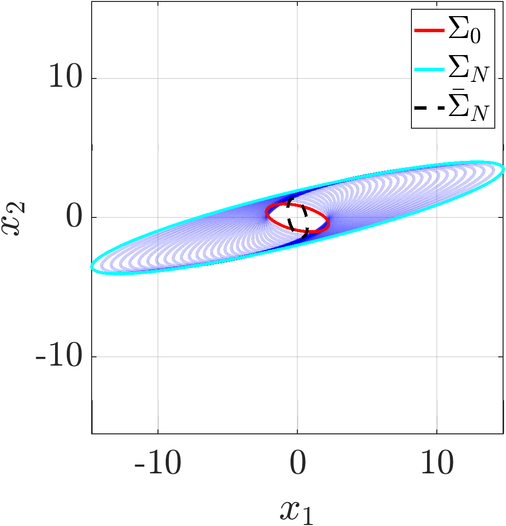
(a) Without feedback control

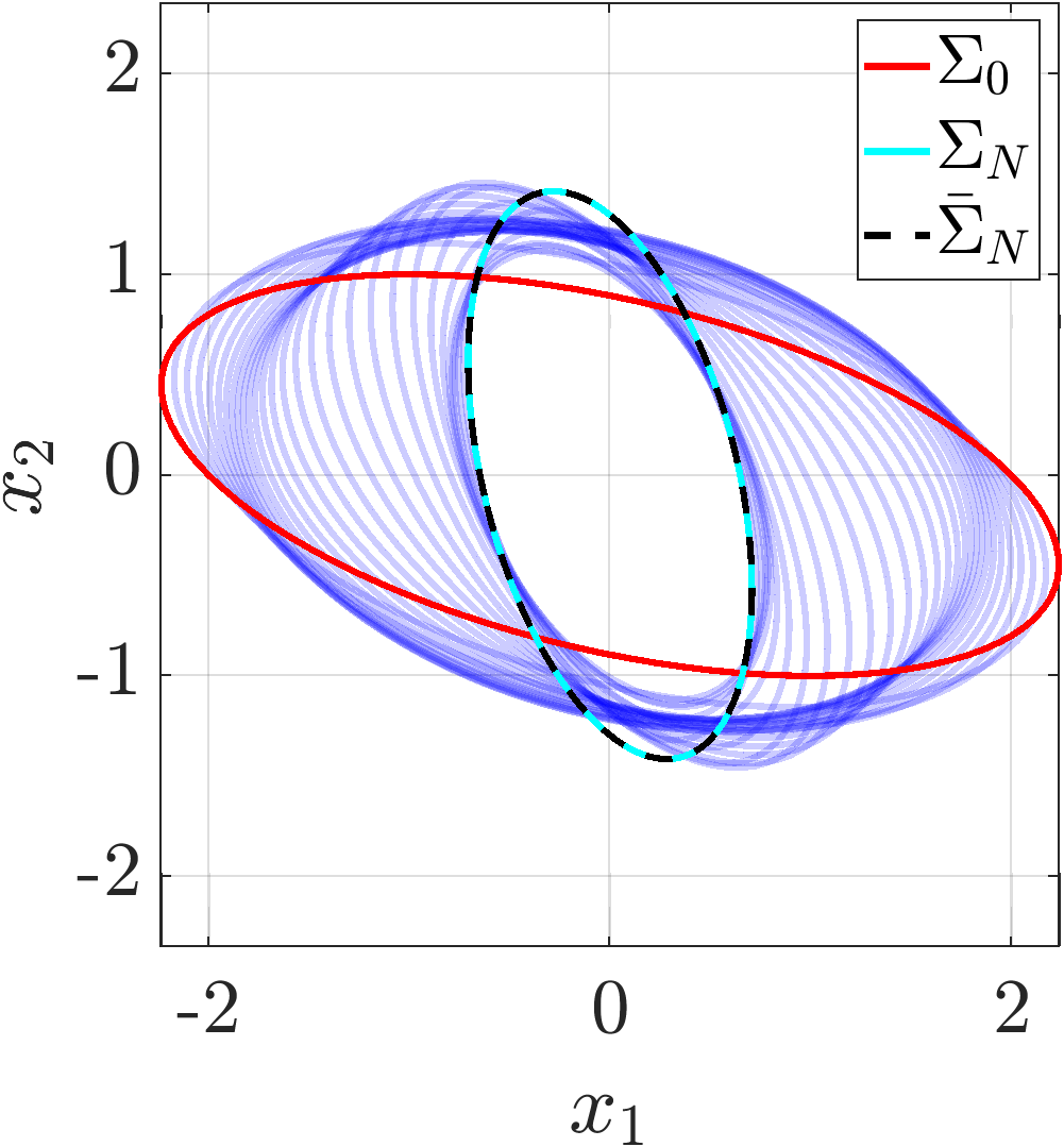
(b) Standard covariance steering

Figure 3: 1-sigma ellipses of the covariance evolution

IV-C Iteratively Reweighted $\ell_{1,p}$ Regularization

Next, we apply the proposed method, i.e. Algorithm 1. We use the parameters $\epsilon=10^{-3}$, $l_{\max}=50$.

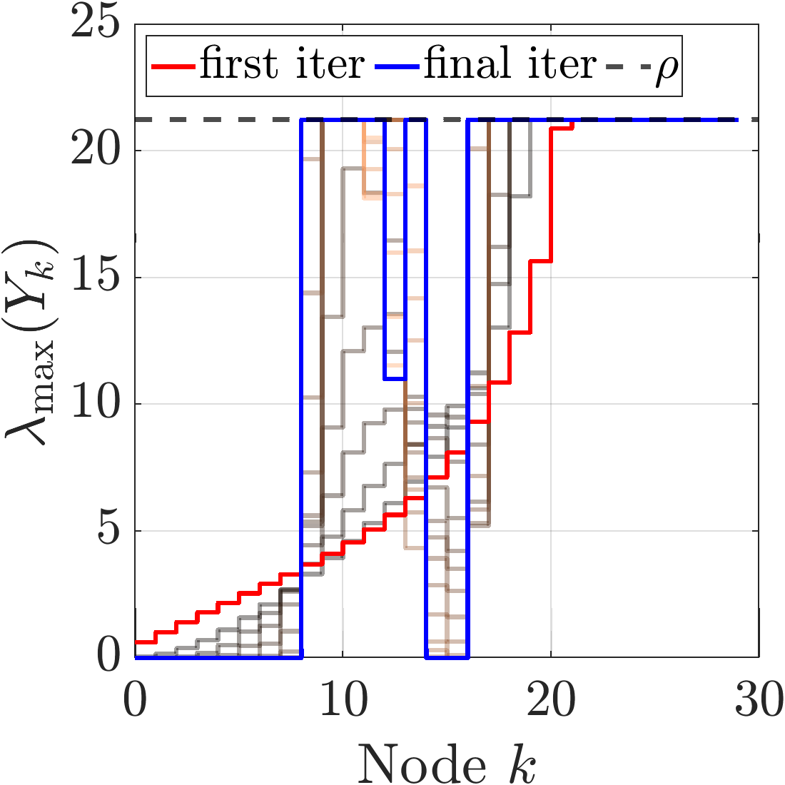
(a) with chance constraints

(b) w/o chance constraints

Figure 4: Control covariance max eigenvalue at each iteration for $\lambda=1000$. Darker colors correspond to earlier iterations.

Fig. 4 shows the value of $\lambda_{\max}(Y_{k})$ at each iteration, for cases with/without chance constraints, when using $\lambda=1000$. Focusing first on Fig. 4(a), we can see that as the iteration progresses, more nodes have $\lambda_{\max}(Y_{k})\approx 0$, i.e. the feedback gain matrices are zero. We can also see the effect of the chance constraints, as the maximum eigenvalue of $Y_{k}$ is bounded. We remark that the converged solution shows bang-bang profile for $\lambda_{\max}(Y_{k})$. This suggests that the equivalence of $\ell_{1}$-optimal control and sparse control shown in [12] extends to the control of the state covariance when the input covariance is bounded. Without chance constraints, the algorithm converges to a solution that uses only 3 statistically large inputs, as shown in Fig. 4(b). Since the chance constraints are not present, these nodes have much larger values of $\lambda_{\max}(Y_{k})$ compared to the constrained case.

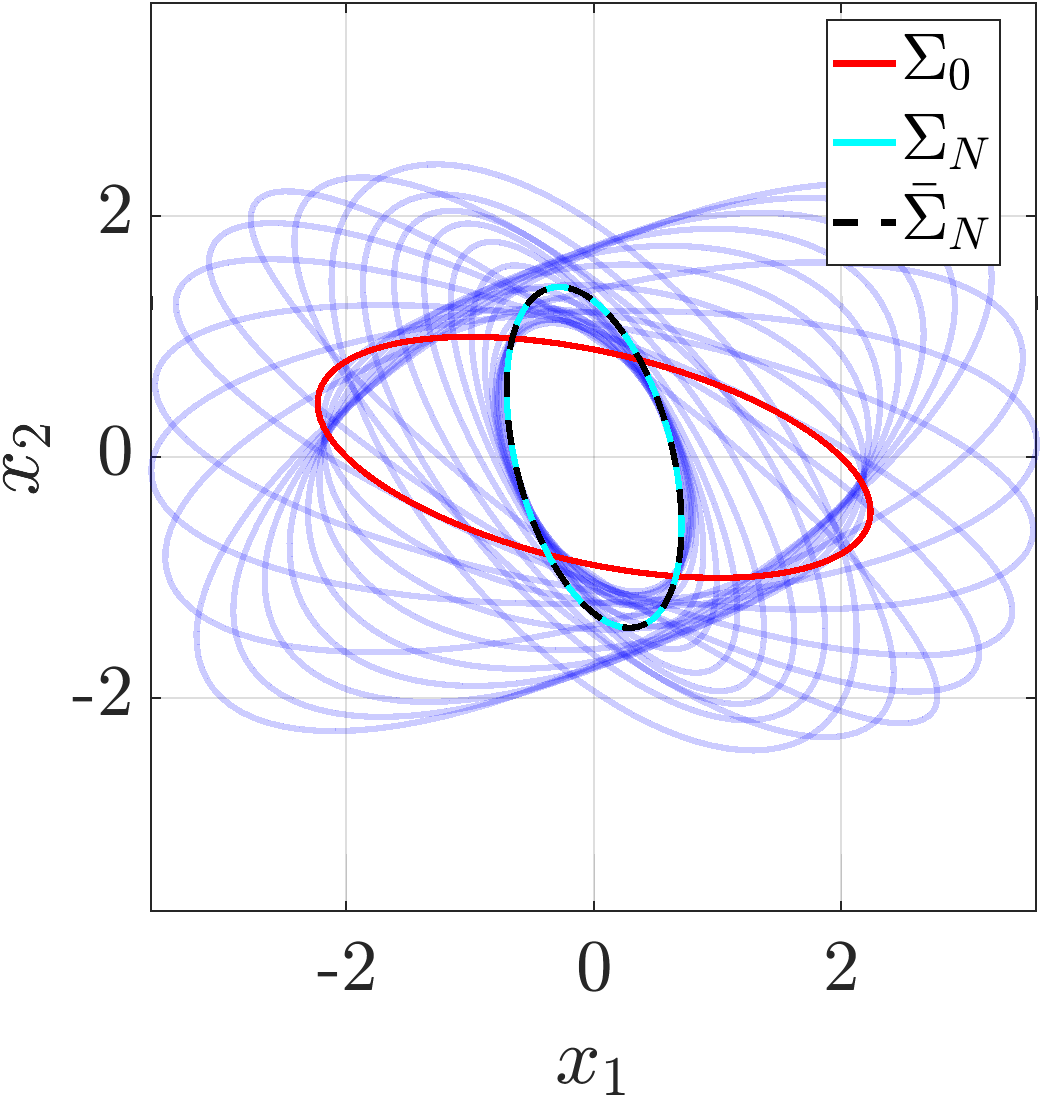
Figure 5: Covariance 1-sigma evolution for IRL1P, $\lambda=1000$

Fig. 5 shows the state covariance evolution. While the covariance ellipse becomes larger compared to the standard covariance steering solution in Fig. 3(b), the final covariance is steered to match the target.

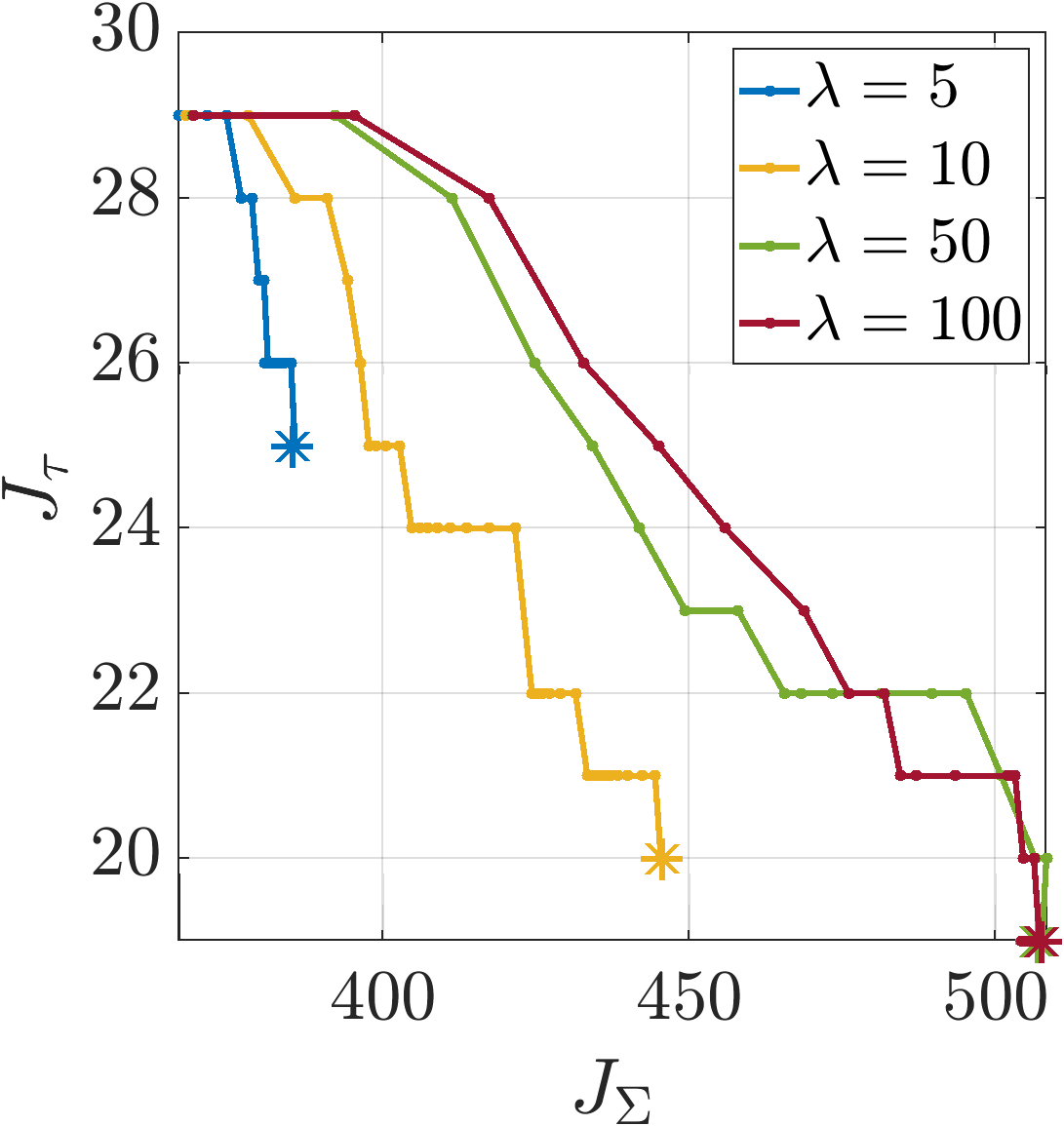
(a)

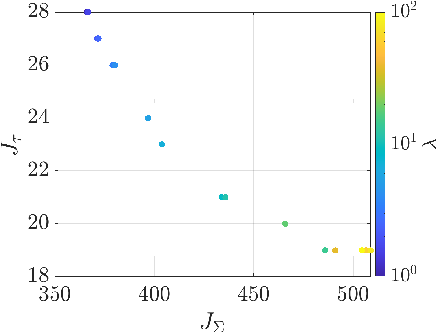
(b)

Figure 6: Left: Algorithm behavior for different $\lambda$. The algorithm starts at the top-left and $*$ shows the final solution. Right: $J_{\Sigma}$ vs $J_{\tau}$ at algorithm termination for different $\lambda$.

Fig. 6(a) shows the transient cost $J_{\Sigma}$ vs the number of nonzero feedback gain matrices $J_{\tau}$ for several values of $\lambda$. As the iteration progresses, the transient cost increases, while sparsity is improved, i.e. the algorithm traverses the line in Fig. 6(a) from top-left to bottom-right. For sufficiently large $\lambda$, (in this case $\lambda=50,100$), the algorithm behavior becomes similar, and increasing $\lambda$ further does not improve sparsity.

Fig. 6(b) shows the $J_{\Sigma}$-$J_{\tau}$ plot at the end of the algorithm for different values of $\lambda$. Here, 20 values of $\lambda$ are chosen to be logarithmically spaced between $1$ and $100$. The plot clearly shows the trade-off between the two objectives based on the value of $\lambda$.

IV-D Ineffectivity of Simple Regularization

Here, we show the result from solving 22, i.e. unweighted regularization. The resulting $\lambda_{\max}(Y_{k})$ for each $k$ is shown in Fig. 7. This example tested $\lambda=10^{4},10^{10}$. For comparison, values from standard covariance steering are also shown. We can see that simple regularization does not induce sparsity in the control input covariance, even for large $\lambda$. This matches the result in Fig. 6(a) for IRL1P, where the first iterations of the algorithm do not improve the sparsity.

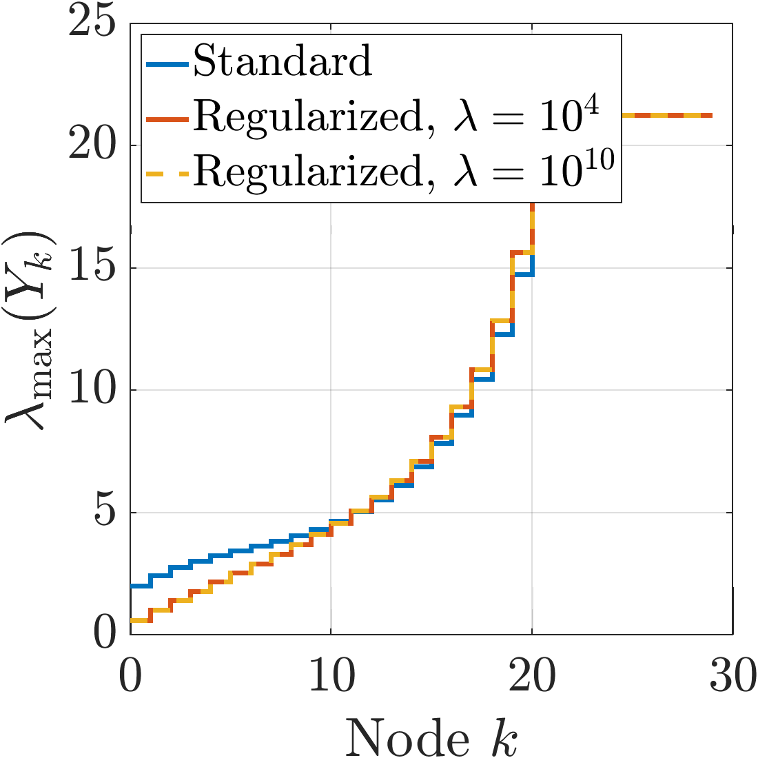
Figure 7: $\lambda_{\max}(Y_{k})$, standard/regularized covariance steering

V Conclusions

We demonstrate chance-constrained, hands-off covariance steering by applying iteratively reweighted $\ell_{1,p}$-norm minimization as a means of approximately solving $\ell_{0}$-norm regularization in the feedback gain matrices. We prove that the lossless convexification property of covariance steering holds under the additional regularization term. The method efficiently explores the trade between transient cost and sparsity in the feedback gain matrices by solving a series of convex optimization problems. Future works include application to path planning under chance constraints and nonlinear dynamics.

References

- [1] B. K. Natarajan, “Sparse Approximate Solutions to Linear Systems,” SIAM J. Comput., vol. 24, pp. 227–234, Apr. 1995.
- [2] R. Tibshirani, “Regression Shrinkage and Selection Via the Lasso,” J. Roy. Statist. Soc.: Ser. B (Methodological), vol. 58, pp. 267–288, Jan. 1996.
- [3] S. S. Chen, D. L. Donoho, and M. A. Saunders, “Atomic Decomposition by Basis Pursuit,” SIAM Rev., vol. 43, pp. 129–159, Jan. 2001.
- [4] E. J. Candès, M. B. Wakin, and S. P. Boyd, “Enhancing Sparsity by Reweighted 1 Minimization,” J Fourier Anal Appl, vol. 14, pp. 877–905, Dec. 2008.
- [5] S. P. Boyd and L. Vandenberghe, Convex Optimization. Cambridge, UK: Cambridge University Press, Mar. 2004.
- [6] S. Boyd, M. T. Mueller, B. O’Donoghue, and Y. Wang, “Performance Bounds and Suboptimal Policies for Multi–Period Investment,” OPT, vol. 1, pp. 1–72, Dec. 2013.
- [7] D. Léonard and N. van Long, Optimal Control Theory and Static Optimization in Economics. Cambridge, UK: Cambridge University Press, 1992.
- [8] K. Oguri, “Chance-Constrained Control for Safe Spacecraft Autonomy: Convex Programming Approach,” in Amer. Control Conf., (Toronto, ON, Canada), pp. 2318–2324, July 2024.
- [9] S. K. Pakazad, H. Ohlsson, and L. Ljung, “Sparse control using sum-of-norms regularized model predictive control,” in 52nd IEEE Conf. Decis. Control, (Firenze, Italy), pp. 5758–5763, Dec. 2013.
- [10] A. Hassibi, J. P. How, and S. P. Boyd, “Low-Authority Controller Design by Means of Convex Optimization,” J. Guid. Control Dyn., vol. 22, pp. 862–872, Nov. 1999.
- [11] H. Ohlsson, F. Gustafsson, L. Ljung, and S. Boyd, “Trajectory generation using sum-of-norms regularization,” in 49th IEEE Conf. Decis. Control, (Atlanta, GA), pp. 540–545, Dec. 2010.
- [12] M. Nagahara, D. E. Quevedo, and D. Nešić, “Maximum Hands-Off Control: A Paradigm of Control Effort Minimization,” IEEE Trans. Automat. Contr., vol. 61, pp. 735–747, Mar. 2016.
- [13] M. R. Jovanović and F. Lin, “Sparse quadratic regulator,” in Eur. Control Conf., (Zurich, Switzerland), pp. 1047–1052, July 2013.
- [14] J. Gao and D. Li, “Cardinality Constrained Linear-Quadratic Optimal Control,” IEEE Trans. Automat. Contr., vol. 56, pp. 1936–1941, Aug. 2011.
- [15] Z. Zhang and M. Nagahara, “Linear Quadratic Tracking Control with Sparsity-Promoting Regularization,” in Amer. Control Conf., (New Orleans, LA), pp. 3812–3817, May 2021.
- [16] A. Hotz and R. E. Skelton, “Covariance control theory,” Int. J. Control, vol. 46, pp. 13–32, July 1987.
- [17] E. Bakolas, “Optimal covariance control for discrete-time stochastic linear systems subject to constraints,” in IEEE 55th Conf. Decis. Control, (Las Vegas, NV), pp. 1153–1158, IEEE, Dec. 2016.
- [18] K. Okamoto, M. Goldshtein, and P. Tsiotras, “Optimal Covariance Control for Stochastic Systems Under Chance Constraints,” IEEE Control Syst. Lett., vol. 2, pp. 266–271, Apr. 2018.
- [19] Y. Chen, T. T. Georgiou, and M. Pavon, “Optimal Steering of a Linear Stochastic System to a Final Probability Distribution—Part III,” IEEE Trans. Automat. Contr., vol. 63, pp. 3112–3118, Sept. 2018.
- [20] F. Liu, G. Rapakoulias, and P. Tsiotras, “Optimal Covariance Steering for Discrete-Time Linear Stochastic Systems,” IEEE Trans. Automat. Contr., pp. 1–16, 2024.
- [21] N. Kumagai and K. Oguri, “Chance-Constrained Gaussian Mixture Steering to a Terminal Gaussian Distribution,” in IEEE 63rd Conf. Decis. Control, (Milan, Italy), pp. 2207–2212, Dec. 2024.
- [22] M. Schmidt, “Lecture Notes for CPSC 5XX - First-Order Optimization Algorithms for Machine Learning: Structured Regularization.” Available: https://www.cs.ubc.ca/~schmidtm/Courses/5XX-S20/S7.pdf.
- [23] M. Yuan and Y. Lin, “Model Selection and Estimation in Regression with Grouped Variables,” J. Roy. Statist. Soc.: Ser. B (Methodological), vol. 68, pp. 49–67, Feb. 2006.
- [24] X. Chen and W. Zhou, “Convergence of the reweighted 1 minimization algorithm for 2–p minimization,” Comput Optim Appl, vol. 59, pp. 47–61, Oct. 2014.
- [25] J. Lofberg, “YALMIP : A toolbox for modeling and optimization in MATLAB,” in IEEE Int. Conf. Robot. Automat., (New Orleans, LA), pp. 284–289, Sept. 2004.
- [26] MOSEK ApS, “The MOSEK optimization toolbox for MATLAB manual. Version 10.2,” 2023. Available: https://docs.mosek.com/latest/toolbox/index.html.
- [27] G. Rapakoulias and P. Tsiotras, “Discrete-Time Optimal Covariance Steering via Semidefinite Programming,” in IEEE 62nd Conf. Decis. Control, pp. 1802–1807, Dec. 2023.