Universal Structure of Computing Moments for Exact Quantum Dynamics: Application to Arbitrary System-Bath Couplings

Abstract

We introduce a general procedure for computing higher-order moments of correlation functions in open quantum systems, extending the scope of our recent work on Memory Kernel Coupling Theory (MKCT) [W. Liu, Y. Su, Y. Wang, and W. Dou, arXiv:2407.01923 (2024)]. This approach is demonstrated for arbitrary system-bath coupling that can be expressed as polynomial, $H_{SB}=\hat{V}(\alpha_{0}+\alpha_{1}\hat{q}+\alpha_{2}\hat{q}^{2}+\dots)$, where we show that the recursive commutators of a system operator obey a universal hierarchy. Exploiting this structure, the higher-order moments are obtained by evaluating the expectation values of the system and bath operators separately, with bath expectation values derived from the derivatives of a generating function. We further apply MKCT to compute the dipole autocorrelation function for the spin-boson model with both linear and quadratic coupling, achieving agreement with the hierarchical equations of motion approach. Our findings suggest a promising path toward accurate dynamics for complex open quantum systems.

I Introduction

The correlation function,

$$C_{AA}(t)\equiv\Tr\left(e^{\textup{i}\hat{H}t}\hat{A}e^{-\textup{i}\hat{H}t}\hat{A}\hat{\rho}_{0}\right),$$ (1)

captures the quantum dynamics of the operator $\hat{A}$ under the Hamiltonian $\hat{H}$ at inverse temperature $\beta$ starting from an initial state $\hat{\rho}_{0}$. It is fundamental to various experimental observables [1] and has recently gained significance in polaritonic chemistry [2, 3, 4], spectroscopy [5, 6, 7], and transport phenomena [8, 9]. In these contexts, the quantum system interacts with a condensed-phase environment consisting of electronic and vibrational degrees of freedom, which can be described by the open quantum system Hamiltonian [10]:

$$\hat{H}=\hat{H}_{S}+\hat{H}_{B}+\hat{H}_{SB},$$ (2)

where $\hat{H}_{S}$ represents the system, $\hat{H}_{B}$ the bath, and $\hat{H}_{SB}$ their interaction.

The significance of $C_{AA}(t)$ in open quantum systems has driven the development of numerous methods, each striking a different balance between accuracy and computational cost. At the high-accuracy end, exact methods [11, 12, 13, 14] can solve small model problems but are computationally prohibitive for larger systems. To enable simulations of more complex and realistic models, various approximation methods have been developed, including perturbative approaches [15, 16], mode-coupling theory [17, 18], semi-classical methods [19, 20, 21], and mixed quantum-classical methods [22, 23, 24, 25]. Despite these advancements, no single approach has achieved the ideal balance between accuracy and efficiency, and the search for improved methods remains an active area of research.

Projection operator techniques [26, 27, 28, 29] are powerful tools for studying open quantum system dynamics. The Mori projection [29], in particular, simplifies the problem by projecting onto the operator of interest, $\hat{A}$, to reduce the dimensionality. This reformulates the computation of $C_{AA}(t)$ into finding the memory kernel, which offers a key advantage in dissipative systems: it typically decays faster than the correlation function itself [30, 31]. However, this approach presents a challenge–the memory kernel depends on the projected propagator [32], which is inherently difficult to handle. Significant efforts have been made to compute the memory kernel [33], including numerically “exact” approaches [34, 30, 35, 36] and various approximation methods [37, 38, 32, 39, 40].

In a recent study [41], we introduced Memory Kernel Coupling Theory (MKCT), a novel approach for computing the memory kernel. MKCT defines a set of auxiliary higher-order memory kernels whose evolution is governed solely by the higher-order moments of the correlation function. Since the higher-order moments are pure static quantities, this means MKCT allows us to obtain the correlation function without explicitly evolving the open quantum system. However, our previous implementation relied on the Liouvillian superoperator from Dissipaton Equations of Motion (DEOM) [14] to compute the moments, limiting the broader applicability of MKCT.

In this article, we present a general procedure for computing correlation function moments to arbitrary order, expanding the applicability of MKCT. We demonstrate our approach using a polynomial bosonic interaction and uncover a universal hierarchy of the recursive commutators of a system operator that determines the moments.

The article is structured as follows: In Sec. II.1, we revisit the MKCT framework and introduce a new Padé arroximation-based truncation scheme. Sec. II.2 presents our novel moments computation procedure. In Sec. III, we apply our method to the spin-boson model with linear, quadratic, and mixed linear-quadratic couping. Finally, we conclude in Sec. IV.

II Theory

II.1 Memory Kernel Coupling Theory

Following Mori’s projection approach, [29] the correlation function in Eq. 1 satisfies the generalized quantum master equation (GQME):

$$\dot{C}_{AA}(t)=\Omega C_{AA}(t)+\int_{0}^{t}\differential{\tau}K(t-\tau)C_{AA}(t),$$ (3)

where the scalar $\Omega$ and the kernel function $K(t)$ are derived from the Mori-Zwanzig formalism:

$$\Omega=(\textup{i}\mathcal{L}\hat{A},A)(\hat{A},\hat{A})^{-1},$$ (4)

$$K(t)=(\textup{i}\mathcal{L}e^{\textup{i}t\bm{\mathcal{Q}}\mathcal{L}}\bm{\mathcal{Q}}\textup{i}\mathcal{L}\hat{A},\hat{A})(\hat{A},\hat{A})^{-1}.$$ (5)

Here, the Mori-product notation $(\hat{A},\hat{B})$ is used to denote some appropriate inner product; the Liouville operator is $\mathcal{L}\square\equiv\frac{1}{\hbar}\commutator{\hat{H}}{\square}$; the projection operator is $\bm{\mathcal{P}}\square=(\square,\hat{A})\hat{A}(\hat{A},\hat{A})^{-1}$; and the projection operator onto the complementary subspace is $\bm{\mathcal{Q}}=\bm{1}-\bm{\mathcal{P}}$.

In practice, $\Omega$ is readily available and many existing works have introduced methods to approximate the kernel function $K(t)$. [38, 32, 42] Recently, we have introduced a novel method called Memory Kernel Coupling Theory (MKCT) to compute $K(t)$ efficiently. [41] Our key idea is to extend the definition of $\Omega$ and $K(t)$ in the Mori GQME and introduce the higher-order moments

$$\Omega_{n}\equiv((\textup{i}\mathcal{L})^{n}\hat{A},\hat{A})(\hat{A},\hat{A})^{-1},$$ (6)

and the corresponding auxiliary kernels

$$K_{n}(t)\equiv((\textup{i}\mathcal{L})^{n}\hat{f}(t),\hat{A})(\hat{A},\hat{A})^{-1},$$ (7)

where the random fluctuation operator is $\hat{f}(t)=e^{\textup{i}t\bm{\mathcal{Q}}\mathcal{L}}\bm{\mathcal{Q}}\textup{i}\mathcal{L}\hat{A}$. We have shown in Ref. [41] that the higher-order kernels satisfy the following coupled ordinary differential equation (ODE):

$$\dot{K}_{n}(t)=K_{n+1}(t)-\Omega_{n}K_{1}(t),$$ (8)

with initial conditions $K_{n}(0)=\Omega_{n+1}-\Omega_{n}\Omega_{1}$. This result is compelling as it reveals that the quantum dynamics can be fully encoded in a system of interconnected ODEs for the higher-order kernels. Notably, the only parameters needed to integrate $\{K_{n}(t)\}$ are $\{\Omega_{n}\}$, meaning that our MKCT framework eliminates the need to explicitly evolve the operator $\hat{A}$ within the open quantum system.

However, a caveat of Eq. 8 is that the equation extends to infinite order, and there is no straightforward method to truncate it at a finite order. From our experience, a hard truncation can lead to numerical instabilities. To this end, we introduce a novel truncation scheme with Padé approximant.

To begin with, notice that the $m$-th derivative of kernel $K_{n}(t)$ evaluated at $t=0$ is

$$K_{n}^{(m)}\equiv((\textup{i}\mathcal{L})^{n}(\bm{\mathcal{Q}}\textup{i}\mathcal{L})^{m+1}\hat{A},\hat{A})(\hat{A},\hat{A})^{-1}.$$ (9)

A recursion relation can be found by expanding $\bm{\mathcal{Q}}=\bm{1}-\bm{\mathcal{P}}$ that

$$K_{n}^{(m)}=K_{n+1}^{(m-1)}-\Omega_{n}\tilde{\Omega}_{m},$$ (10)

where we have introduced the auxiliary moment

$$\tilde{\Omega}_{m}=(\textup{i}\mathcal{L}(\bm{\mathcal{Q}}\textup{i}\mathcal{L})^{m}\hat{A},\hat{A})(\hat{A},\hat{A})^{-1}.$$ (11)

Recursively applying Eq. 10 eventually leads the following expression:

$$K_{n}^{(m)}=\Omega_{m+n+1}-\Omega_{n}\tilde{\Omega}_{m}-\dots-\Omega_{m+n}\tilde{\Omega}_{0},$$ (12)

that $K_{n}^{(m)}$ can be expressed with moments and auxiliary moments. Similarly, the auxiliary moments themselves have recursions

$$\tilde{\Omega}_{m} =(\textup{i}\mathcal{L}(\bm{\mathcal{Q}}\textup{i}\mathcal{L})^{m-1}\textup{i}\mathcal{L}\hat{A},\hat{A})(\hat{A},\hat{A})^{-1}-\tilde{\Omega}_{m-1}\Omega_{1},$$ (13)

$$=\Omega_{m+1}-\tilde{\Omega}_{m}\Omega_{1}-\dots\tilde{\Omega}_{1}\Omega_{m},$$

which means the auxiliary moments $\{\tilde{\Omega}_{m}\}$ can be readily obtained by the moments $\{\Omega_{n}\}$.

The series expansion for the $n$-th order kernel can then be given by Padé approximant. Initially, $K_{n}(t)$ is expressed as a truncated Taylor series:

$$K_{n}(t)\approx\sum_{j=0}^{M}\frac{K_{n}^{(j)}(0)}{j!}t^{j},$$ (14)

which is a good local approximation but lacks accuracy over a broader range of $t$. A more reliable approximation can be achieved using the Padé approximant:

$$K_{n}(t)\approx\frac{p_{M_{1}}(t)}{q_{M_{2}}(t)}=\frac{a_{0}+a_{1}t+\dots+a_{M_{1}}t^{M_{1}}}{1+b_{1}t+\dots+b_{M_{2}}t^{M_{2}}},$$ (15)

where $p_{M_{1}}(t)$ and $q_{M_{2}}(t)$ are polynomials of degrees $M_{1}$ and $M_{2}$, respectively. The coefficients $\{a_{i}\}$and $\{b_{i}\}$ are determined following the standard procedure [43]. Overall, Eq. 15 provides a numerically stable truncation for the MKCT Eq. 8, where all coefficients can be evaluated with higher-order moments $\{\Omega_{n}\}$.

II.2 Moments for A General System-Bath Model: Polynomial Interaction

To study the dynamics of a discrete quantum system coupled to a vibrational environment, the following model is commonly used:

$$\hat{H}=\hat{H}_{S}+\sum_{j}\frac{\hbar\omega_{j}}{2}(\hat{p}_{j}^{2}+\hat{q}_{j}^{2})+\hat{V}U(\hat{q}),$$ (16)

where ${\hat{q}_{j}}$ and $\hat{p}_{j}$ are the position and momentum operators for the $j$-th mode of a harmonic bath with frequency $\omega_{j}$, and $U(\hat{q})$ represents arbitrary potential energy that can be expressed in polynomial

$$U(\hat{q})=\alpha_{0}+\alpha_{1}\hat{q}+\alpha_{2}\hat{q}^{2}+\dots$$ (17)

The system is coupled to a polynomial of the collective mode, $\hat{q}=\sum_{j}c_{j}\hat{q}_{j}$, which is characterized by the spectral density:

$$J(\omega)=\frac{\pi}{2}\sum_{j}c_{j}^{2}\delta(\omega-\omega_{j}).$$ (18)

Most studies only consider linear coupling, but a growing body of research shows the significance of non-linear interactions [44, 45, 46, 47, 48]. Here, we consider a general polynomial coupling with coefficients $\{\alpha_{i}\}$.

Suppose that $\hat{A}$ is the system operator of interest, applying the MKCT to calculate $C_{AA}(t)$ boils down to 1) Compute $(\textup{i}\mathcal{L})^{n}\hat{A}$ to arbitrary order. 2) Evaluate the inner product $((\textup{i}\mathcal{L})^{n}\hat{A},\hat{A})$. In this work, we define the Mori-product as

$$(\hat{A},\hat{B})=\Tr(\hat{A}\hat{B}\hat{\rho}_{0}\otimes\hat{\rho}_{\text{eq}}^{B}),$$ (19)

where we assume a factorized initial condition. Here, $\hat{\rho}_{0}$ is the initial system density operator, and $\hat{\rho}_{\text{eq}}^{B}=e^{-\beta\hat{H}_{B}}/\Tr(e^{-\beta\hat{H}_{B}})$ is the equilibrium bath density operator.

II.2.1 The Application of Liouvillian

To compute $(\textup{i}\mathcal{L})^{n}\hat{A}$ to arbitrary order, we begin by writing down the first few terms and recognizing the following pattern:

$$(\textup{i}\mathcal{L})^{n}\hat{A}=\sum_{\text{all terms}}\hat{O}\otimes\prod_{j}\hat{Q}_{m_{j}}\prod_{k}\hat{P}_{n_{k}},$$ (20)

where each term is a product of a system operator $\hat{O}$ and a polynomial of bath operators. Note that we have introduced the following generalized bath mode operators,

$$\hat{Q}_{m}=\sum_{j}c_{j}\omega_{j}^{m}\hat{q}_{j},$$ (21)

$$\hat{P}_{n}=\sum_{j}c_{j}\omega_{j}^{n}\hat{p}_{j},$$ (22)

to simplify the notation in Eq. 20. The polynomial is organized so that the position operators $\hat{Q}_{m}$ always appear before the momentum operators $\hat{P}_{n}$. Note that the collective mode $\hat{q}\equiv\hat{Q}_{0}$. For brevity, the direct product symbol $\otimes$ is omitted henceforth.

In order to verify that the general pattern of Eq. 20 is closed and to outline a practical procedure for computing $(\textup{i}\mathcal{L})^{n}\hat{A}$, we demonstrate below how applying the Liouvillian $\textup{i}\mathcal{L}=\textup{i}\mathcal{L}_{S}+\textup{i}\mathcal{L}_{B}+\textup{i}\mathcal{L}_{SB}$ to a general term generates a set of new terms. To formalize this, we denote a general term by $\hat{G}=\hat{O}\prod_{j}\hat{Q}_{m_{j}}\prod_{k}\hat{P}_{n_{k}}$.

To begin with, the application of $\textup{i}\mathcal{L}_{S}$ is straightforward:

$$\textup{i}\mathcal{L}_{S}\hat{G}=\textup{i}\commutator{\hat{H}_{S}}{\hat{O}}\prod_{j}\hat{Q}_{m_{j}}\prod_{k}\hat{P}_{n_{k}}.$$ (23)

Next, we utilize the properties of the harmonic bath outlined in Eqs. 39 and 40, along with the commutation relation $\commutator{A}{BC}=\commutator{A}{B}C+B\commutator{A}{C}$, to write

$$\textup{i}\mathcal{L}_{B}\hat{G}=\hat{O}\left[\sum_{\alpha}\left(\prod_{j_{1}<\alpha}\hat{Q}_{m_{j_{1}}}\right)\hat{P}_{m_{\alpha}}\left(\prod_{j_{2}>\alpha}\hat{Q}_{m_{j_{2}}}\right)\right]\prod_{k}\hat{P}_{n_{k}}\\ -\hat{O}\prod_{j}\hat{Q}_{m_{j}}\left[\sum_{\alpha}\left(\prod_{k_{1}<\alpha}\hat{P}_{n_{\alpha}}\right)\hat{Q}_{m_{\alpha}+2}\left(\prod_{k_{2}>\alpha}\hat{P}_{m_{k_{2}}}\right)\right].$$ (24)

Note that the terms in Eq. 24 differ from the general form in Eq. 20 because the $\hat{Q}_{n}$ terms do not always appear before the $\hat{P}_{n}$ terms. To this end, Eq. 24 can be further ordered using the following procedures:

$$\hat{P}_{n}\prod_{j}\hat{Q}_{{m}_{j}}=\prod_{j}\hat{Q}_{{m}_{j}}\hat{P}_{n}+\sum_{\alpha}(-\textup{i}\theta_{n+m_{\alpha}})\prod_{j\neq\alpha}\hat{Q}_{{m}_{j}},$$ (25)

$$\prod_{k}\hat{P}_{n_{k}}\hat{Q}_{m}=\hat{Q}_{m}\prod_{k}\hat{P}_{n_{k}}+\sum_{\alpha}(-\textup{i}\theta_{m+n_{\alpha}})\prod_{k\neq\alpha}\hat{P}_{{n}_{k}},$$ (26)

where we have used the harmonic bath property from Eq. 41 and the identity $\hat{A}\hat{B}=\hat{B}\hat{A}+\commutator{\hat{A}}{\hat{B}}$. Note that we have introduced we introduce the function $\theta_{n}$,

$$\theta_{n}=\frac{2}{\pi}\int_{0}^{\infty}\differential{\omega}J(\omega)\omega^{n},$$ (27)

to simplify the notation. Lastly, we expand the commutator $\textup{i}\mathcal{L}_{SB}$:

$$\textup{i}\mathcal{L}_{SB}\hat{G}=\textup{i}\hat{V}\hat{O}U(\hat{q})\prod_{j}\hat{Q}_{m_{j}}\prod_{k}\hat{P}_{n_{k}}-\textup{i}\hat{O}\hat{V}\prod_{j}\hat{Q}_{m_{j}}\prod_{k}\hat{P}_{n_{k}}U(\hat{q}),$$ (28)

In the second term in Eq. 28, the potential operator $U(\hat{q})$ appears after the momentum operators, which is not ordered in the same way as the general term (Eq. 20). However, this term can be brought into the desired order by recursively applying Eq. 26.

Overall, Eqs. 23-26 and Eq. 28 demonstrate that the complete structure of $(\textup{i}\mathcal{L})^{n}\hat{A}$ is captured by the general expression (Eq. 20). This hierarchical structure is universal for a system-bath model with arbitrary electron-phonon coupling potential (Eq. 16, 17), which can be recursively computed up to any arbitrary order $n$.

II.2.2 The Mori Products

To evaluate the moments $\Omega_{n}$ (Eq. 6), we must compute the Mori product between $(\textup{i}\mathcal{L})^{n}\hat{A}$ and $\hat{A}$. This reduces to summing the Mori products of general terms $\{\hat{G}\}$ and $\hat{A}$, where how to obtain the general terms $\hat{G}$ is described in Sec. II.2.1. These Mori products naturally decompose into separate system and bath expectation values:

$$(\hat{G},\hat{A})=\Tr(\hat{O}\hat{A}\hat{\rho}_{0})\Tr(\prod_{j}\hat{Q}_{m_{j}}\prod_{k}\hat{P}_{n_{k}}\hat{\rho}_{\text{eq}}^{B}).$$ (29)

The first trace on the right-hand side (RHS) of Eq. 29 is straightforward to evaluate. However, the second trace, involving bath operator polynomials, is somewhat cumbersome to evaluate.

In order to compute the expectation value of a bath polynomial, we define the following generating function $f(\{\lambda_{\alpha}\},\{\lambda_{\gamma}^{\prime}\})$:

$$f(\{\lambda_{\alpha}\},\{\lambda_{\gamma}^{\prime}\})=\Tr[\exp(\sum_{\gamma}\lambda^{\prime}_{\gamma}\hat{P}_{n_{\gamma}})\hat{\rho}_{\text{eq}}^{B}\exp(\sum_{\alpha}\lambda_{\alpha}\hat{Q}_{m_{\alpha}})],$$ (30)

such that the second trace in Eq. 29 becomes the derivatives of the generating function $f(\{\lambda_{\alpha}\},\{\lambda_{\gamma}^{\prime}\})$

$$\Tr(\prod_{j}\hat{Q}_{m_{j}}\prod_{k}\hat{P}_{n_{k}}\hat{\rho}_{\text{eq}}^{B})=\prod_{\alpha}\derivative{\lambda_{\alpha}}\evaluated{}_{\lambda_{\alpha}=0}\prod_{\gamma}\derivative{\lambda_{\gamma}^{\prime}}\evaluated{}_{\lambda_{\gamma}^{\prime}=0}f(\{\lambda_{\alpha}\},\{\lambda_{\gamma}^{\prime}\}).$$ (31)

As detailed in Appendix B, the generating function has the closed-form expression

$$f(\{\lambda_{\alpha}\},\{\lambda_{\gamma}^{\prime}\})=\exp[\sum_{\alpha}\sum_{\alpha^{\prime}}\frac{\lambda_{\alpha}\lambda_{\alpha^{\prime}}}{2}\eta_{m_{\alpha}+m_{\alpha^{\prime}}}]\times\\ \exp[\sum_{\gamma}\sum_{\gamma^{\prime}}\frac{\lambda_{\gamma}^{\prime}\lambda_{\gamma^{\prime}}^{\prime}}{2}\eta_{n_{\gamma}+n_{\gamma^{\prime}}}]\exp[\textup{i}\sum_{\alpha}\sum_{\gamma}\frac{\lambda_{\alpha}\lambda_{\gamma}^{\prime}}{2}\theta_{m_{\alpha}+n_{\gamma}}],$$ (32)

where the function $\eta_{n}$ is defined as

$$\eta_{n}=\frac{2}{\pi}\int_{0}^{\infty}\differential{\omega}J(\omega)\omega^{n}\coth(\frac{\hbar\omega\beta}{2}).$$ (33)

II.3 Workflow and comments

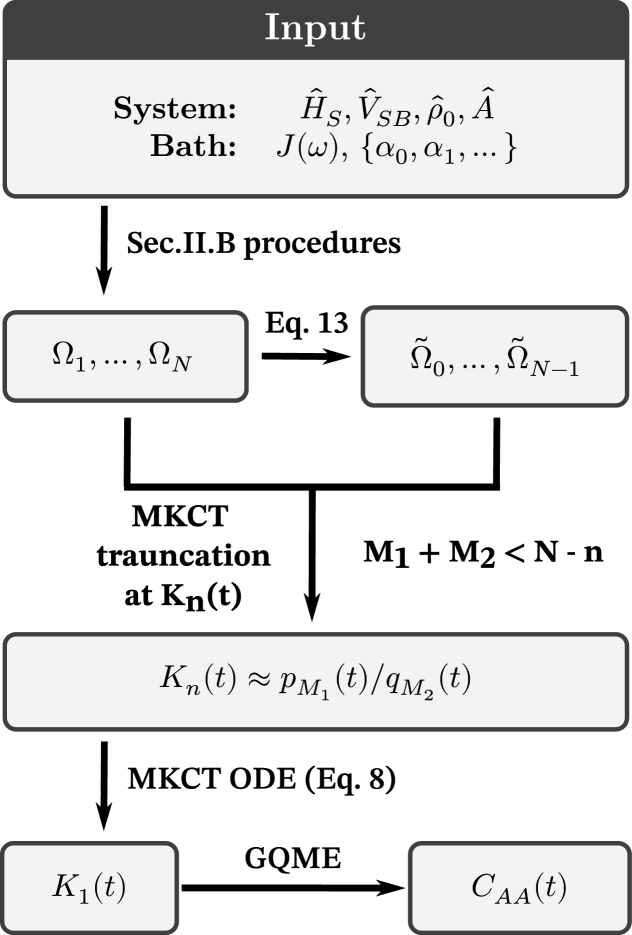
Figure 1: Schematic illustration of the workflow for computing the correlation function using the framework introduced in this work.

We summarize the workflow of our novel framework for computing the correlation function in FIG. 1. Notably, the computation does not require simulating open quantum system dynamics. Instead, the moments $\{\Omega_{n}\}$ are computed statically under the factorized initial condition. Furthermore, the complexity of the hierarchical structure of $(\textup{i}\mathcal{L})^{n}\hat{A}$ remains independent of the basis size of $\hat{A}$. This suggests that our approach can be applied to larger problems where accurate non-Markovian methods, such as the Hierarchical Equations of Motion, become computationally infeasible.

III Numerical Example

In the following, we apply our MKCT framework (Sec. II.1) to compute correlation functions, where the correlation function moments $\Omega_{n}$ are obtained using the methods introduced in Sec. II.2. Throughout Sec. III, we adopt the Ohmic spectral density

$$J(\omega)=2\lambda\omega e^{-\absolutevalue{\omega}/\omega_{D}},$$ (34)

where $\lambda$ is a coefficient with units of inverse frequency squared, ensuring that $J(\omega)$ has units of inverse frequency. The parameter $\omega_{D}$ represents the cutoff frequency. In our examples, we set $\hbar=1$. The system Hamiltonian $\hat{H}_{S}$ has units of energy, the system-bath coupling operator $\hat{V}$ is dimensionless, and the polynomial coefficients $\{\alpha_{i}\}$ have the dimension of energy.

We investigate the dipole autocorrelation function, defined as $C_{\mu\mu}(t)=\expectationvalue{\hat{\mu}(t)\hat{\mu}(0)}$ where the dipole operator is given by $\hat{\mu}=\hat{\sigma}_{x}$. The correlation function $C_{\mu\mu}(t)$ plays a crucial role in spectroscopy, as the absorption lineshape function $I(\omega)$ is directly proportional to its Fourier transform [6]:

$$I(\omega)\propto\real\int_{0}^{\infty}\differential{t}C_{\mu\mu}(t)e^{\textup{i}\omega t}.$$ (35)

As a reference, we use the Dissipaton Equations of Motion (DEOM) approach [14] for linear system-bath coupling (Sec.III.1) and the extended DEOM approach [44] for quadratic system-bath coupling (Sec.III.2). To efficiently decompose the bath correlation function, we employ the time-domain Prony method [49].

III.1 Spin-boson model with linear interaction

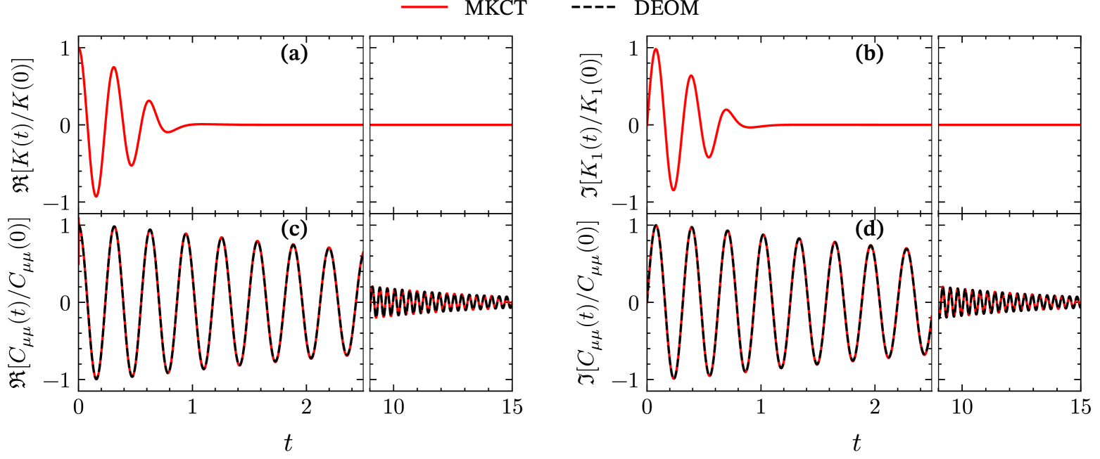
Figure 2: Memory kernel $K_{1}(t)$ and autocorrelation function $C_{\mu\mu}(t)$ for the spin–boson model with linear interaction. (a-b) are the real and complex part of $K_{1}(t)$, respectively. (c-d) are the real and complex part of $C_{\mu\mu}(t)$, respectively. The parameters used are $\alpha_{0}=\alpha_{2}=0$, $\alpha_{1}=1$, $\Delta=20$, $\lambda=0.5$, $\omega_{D}=1$, and $\beta=5$. The Padé orders $n=1$, $M_{1}=7$ and $M_{2}=15$.

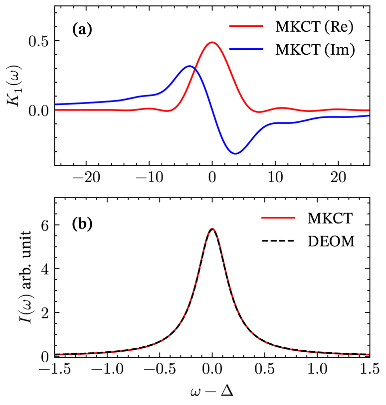
Figure 3: Frequency domain (a) memory kernel $K_{1}(\omega)$ and (b) absorption lineshape $I(\omega)$ for the spin–boson model with linear interaction. The parameters are the same as those in FIG. 2.

We consider a system Hamiltonian $\hat{H}_{S}=\frac{\Delta}{2}\sigma_{z}$, a coupling operator $\hat{V}=\sigma_{z}$, and an initial state $\hat{\rho}_{0}=\outerproduct{0}{0}$. FIG. 2 presents $K_{1}(t)$ and $C_{\mu\mu}(t)$ for an energy gap of $\Delta=20$, demonstrating that our MKCT approach matches the DEOM results exactly. Due to the large energy gap, the correlation function exhibits rapid oscillations, but FIG. 2 shows that $K_{1}(t)$ decays to zero much faster than $C_{\mu\mu}(t)$. This highlights the advantage of computing the memory kernel $K_{1}(t)$, as it captures the dynamics over a shorter timescale. FIG. 3 presents the frequency-domain representations $K_{1}(\omega)$ and $I(\omega)$, showing that the memory kernel $K_{1}(\omega)$ distribution is much more dispersed than the lineshape function $I(\omega)$. This broader distribution suggests that the memory kernel encodes a wider range of dynamical frequencies, which facilitates efficient modeling of non-Markovian effects.

III.2 Spin-boson model with quadratic interaction

Here, we consider a quadratic interaction case adopting the model in Ref. [44]. Specifically, we consider a system Hamiltonian $\hat{H}_{S}=\omega_{eg}\outerproduct{1}{1}$, a coupling operator $\hat{V}=\outerproduct{1}{1}$, and initial state $\hat{\rho}_{0}=\outerproduct{0}{0}$.

FIG. 4 plots $K_{1}(t)$ and $C_{\mu\mu}(t)$ for a purely quadratic system-bath interaction. The dynamics induced by $\hat{q}^{2}$-coupling are known to be highly oscillatory and decay slowly [50, 48]. However, by leveraging a short-timescale memory kernel, our MKCT approach accurately captures the long-time behavior of $C_{\mu\mu}(t)$. When both linear and quadratic interactions are present, the linear coupling introduces an additional dissipation channel, leading to a faster decay of $C_{\mu\mu}(t)$, as shown in FIG. 5. This effect is correctly captured by our MKCT framework. The difference between purely quadratic dynamics and mixed linear-quadratic dynamics is clearly reflected in the absorption lineshape, with the former exhibiting a more localized peak. As shown in FIG. 6, our MKCT approach accurately captures both the peak position and linewidth.

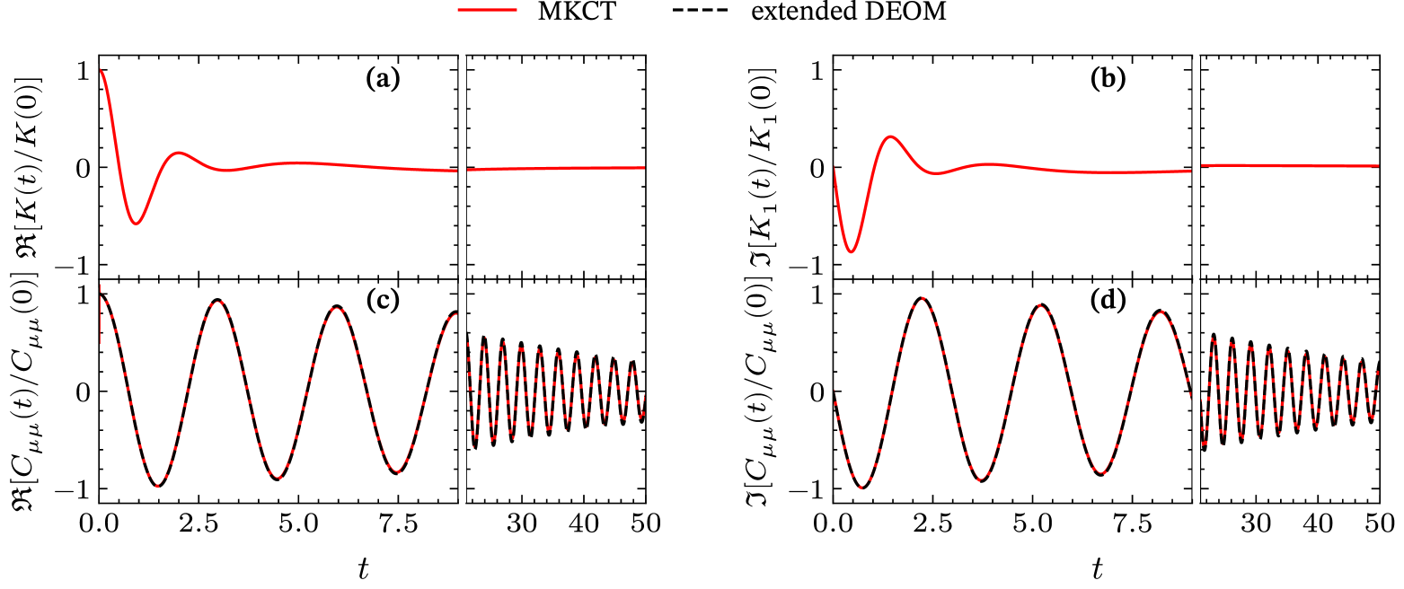
Figure 4: $K_{1}(t)$ and $C_{\mu\mu}(t)$ of the spin–boson model with purely quadratic interaction. (a-d) follow the panel conventions in FIG. 2. The parameters used are $\alpha_{0}=\alpha_{1}=0$, $\alpha_{2}=0.384$, $\omega_{eg}=2$, $\lambda=0.5$, $\omega_{D}=0.5$, and $\beta=1$. The Padé orders $n=1$, $M_{1}=7$ and $M_{2}=8$.

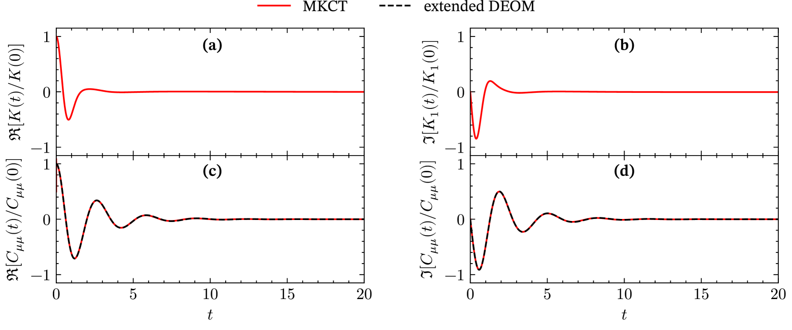
Figure 5: $K_{1}(t)$ and $C_{\mu\mu}(t)$ of the spin–boson model with purely quadratic interaction. (a-d) follow the panel conventions in FIG. 2. The parameters used are $\alpha_{0}=0.442$, $\alpha_{1}=-1.251$, $\alpha_{2}=0.384$ , $\omega_{eg}=2$, $\lambda=0.5$, $\omega_{D}=0.5$, and $\beta=1$. The Padé orders $n=1$, $M_{1}=6$ and $M_{2}=9$.

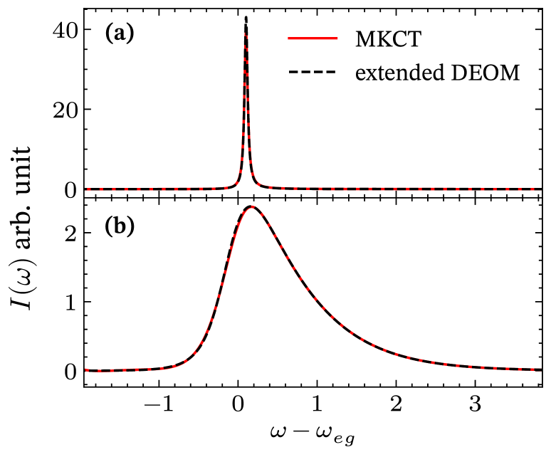
Figure 6: The absorption lineshape $I(\omega)$ of the spin–boson model with quadratic interaction. (a) corresponds to the pure quadratic interaction, with parameters given in FIG. 4. (b) represents the mixed linear-quadratic interaction, with parameters given in FIG. 5

IV Conclusions

We have introduced a novel procedure for computing higher-order moments of correlation functions in open quantum systems with polynomial bosonic coupling. By integrating this approach with Memory Kernel Coupling Theory, we efficiently obtain the memory kernel without explicitly evolving the open quantum system. The faster decay of the memory kernel enables the computation of correlation functions over longer timescales. Our approach allows simulation of the spin-boson model with both linear and quadratic coupling, achieving agreement with numerically “exact” methods.

In this work, we focus on the autocorrelation function with factorized initial conditions. However, our formulation can readily generalize to other types of correlation functions (see Ref. [41]). Moreover, the Mori-based GQME with factorized initial conditions is formally equivalent to the Zwanzig formulation of the GQME for non-equilibrium dynamics [38, 32]. If one is interested in correlation functions with the true equilibrium density, this framework can be extended to multiple-time correlation functions.

It is also worth noting that our method does not rely on a system-bath separation or the assumption of harmonic baths. This flexibility makes it potentially applicable to complex systems, such as bosonic interactions with anharmonic baths or fermionic systems with electron-electron interactions, including Fermi gases and the Hubbard model. These systems are challenging to treat with hierarchical equations of motion but may be more accessible through our MKCT approach. However, computing moments for such cases is more difficult within the current framework, and modifications to our procedure may be necessary. Work is ongoing to extend and refine these methods for broader applicability.

Data Availability

The data and code implementing the theory presented in Sec. II are available from the corresponding author upon reasonable request.

Appendix A Properties of Harmonic Bath

The bare harmonic bath Hamiltonian is given by

$$\hat{H}_{B}=\sum_{j}\frac{\hbar\omega_{j}}{2}(\hat{p}_{j}^{2}+\hat{q}_{j}^{2})=\sum_{j}\hbar\omega_{j}(\hat{b}_{j}^{\dagger}\hat{b}_{j}+1/2),$$ (36)

where the bath mode operators can be represented in ladder operators

$$\hat{q}_{j}\equiv\frac{\hat{b}_{j}^{\dagger}+\hat{b}_{j}}{\sqrt{2}},\quad\hat{p}_{j}\equiv\frac{\hat{b}_{j}-\hat{b}_{j}^{\dagger}}{\textup{i}\sqrt{2}}.$$ (37)

It is straightforward to show

$$\textup{i}\mathcal{L}_{B}\hat{q}_{j}=\omega_{j}\hat{p}_{j},\quad\textup{i}\mathcal{L}_{B}\hat{p}_{j}=-\omega_{j}\hat{q}_{j}.$$ (38)

With properties Eqs. 38, we can derive the following results for the generalized bath modes $\hat{Q}_{m}$ and $\hat{P}_{n}$:

$$\textup{i}\mathcal{L}_{B}\hat{Q}_{m}=\hat{P}_{m+1},$$ (39)

$$\textup{i}\mathcal{L}_{B}\hat{P}_{m}=-\hat{Q}_{m+1},$$ (40)

$$\commutator{\hat{Q}_{m}}{\hat{P}_{n}}=\frac{2\textup{i}}{\pi}\int_{0}^{\infty}\differential{\omega}J(\omega)\omega^{m+n},$$ (41)

Appendix B Derivation of the Generating Function Eq. 32

In order to evaluate the generating function Eq. 30, we start by showing the following operator identity:

$$\hat{\rho}_{\text{eq}}^{B}e^{\kappa\hat{q}_{j}}e^{\chi\hat{p}_{j}}=Z^{-1}\Tr[-\beta\hat{H}_{B}+\frac{x_{j}}{2}\left[(\kappa\coth\frac{x_{j}}{2}-\textup{i}\chi)\hat{q}_{j}+(\textup{i}\kappa+\chi\coth\frac{x_{j}}{2})\hat{p}_{j}\right]]\times\\ \exp[-\frac{x_{j}\beta(\kappa^{2}+\chi^{2})}{8\sinh^{2}(x_{j}/2)}]\exp[\frac{\kappa^{2}+\chi^{2}}{4}\coth(\frac{x_{j}}{2})]\exp[\textup{i}\frac{\kappa\chi}{2}],$$ (42)

where $\kappa$ and $\chi$ are arbitrary scalars, $x_{j}=\hbar\omega_{j}\beta$, and $Z=\Tr[e^{-\beta\hat{H}_{B}}]$ is the bath partition function.

To show Eq. 42, we begin by substituting the ladder operator definitions (Eq. 37) for $\hat{q}_{j}$ and $\hat{p}_{j}$ into the expression. Using the identity $e^{\hat{A}}e^{\hat{B}}=e^{\hat{A}+\hat{B}+\commutator{\hat{A}}{\hat{B}}/2}$ when $\commutator{\hat{A}}{\hat{B}}$ is a constant, we obtain

$$e^{\kappa\hat{q}_{j}}e^{\chi\hat{p}_{j}}=\exp[\frac{(\kappa-\textup{i}\chi)}{\sqrt{2}}\hat{b}_{j}]\exp[\frac{(\kappa-\textup{i}\chi)}{\sqrt{2}}\hat{b}_{j}]\exp(-\frac{\kappa^{2}+\chi^{2}}{4}+\textup{i}\frac{\kappa\chi}{2}).$$ (43)

Then, we utilize the identity $e^{\hat{A}}e^{\hat{B}}=\exp(\hat{A}+\frac{s}{1-e^{-s}}\hat{B})$ when $\commutator{\hat{A}}{\hat{B}}=s\hat{B}$ consecutively to show that

$$\exp[-x_{j}\left(\hat{b}_{j}^{\dagger}\hat{b}_{j}+\frac{1}{2}\right)]\exp[\frac{(\kappa-\textup{i}\chi)}{\sqrt{2}}\hat{b}_{j}]=\\ \exp[-x_{j}\left(\hat{b}_{j}^{\dagger}\hat{b}_{j}+\frac{1}{2}\right)+\frac{x_{j}}{1-e^{-x_{j}}}\frac{(\kappa-\textup{i}\chi)}{\sqrt{2}}\hat{b}_{j}],$$ (44)

and

$$\exp[-x_{j}\left(\hat{b}_{j}^{\dagger}\hat{b}_{j}+\frac{1}{2}\right)+\frac{x_{j}}{1-e^{-x_{j}}}\frac{(\kappa-\textup{i}\chi)}{\sqrt{2}}\hat{b}_{j}]\exp[\frac{(\kappa+\textup{i}\chi)}{\sqrt{2}}\hat{b}_{j}^{\dagger}]\exp[-\frac{\kappa^{2}+\chi^{2}}{2(1-e^{-x_{j}})}]=\\ \exp[-x_{j}\left(\hat{b}_{j}^{\dagger}\hat{b}_{j}+\frac{1}{2}\right)+\frac{x_{j}}{1-e^{-x_{j}}}\frac{(\kappa-\textup{i}\chi)}{\sqrt{2}}\hat{b}_{j}+\frac{-x_{j}}{1-e^{x_{j}}}\frac{(\kappa+\textup{i}\chi)}{\sqrt{2}}\hat{b}_{j}^{\dagger}]\times\\ \exp[-\frac{-x_{j}}{1-e^{x_{j}}}\frac{\kappa^{2}+\chi^{2}}{2(1-e^{-x_{j}})}].$$ (45)

Finally, we notice that the second and third terms in the first exponential on the right-hand side of Eq. 45 follow the pattern $a\hat{X}+(a-1)\hat{X}^{\dagger}$, where $a=(1-e^{-x_{j}})^{-1}$ and $\hat{X}=\frac{\kappa-\textup{i}\chi}{\sqrt{2}}\hat{b}_{j}$. Utilizing the identity $a\hat{X}+(a-1)\hat{X}^{\dagger}=\frac{1}{2}(\hat{X}-\hat{X}^{\dagger})+(a-\frac{1}{2})(\hat{X}+\hat{X}^{\dagger})$, we can re-express Eq. 45 in terms of $\hat{q}_{j}$ and $\hat{p}_{j}$. Combining Eqs. 43, 44, and 45, we derive the operator identity Eq. 42.

We then directly apply Eq. 42 to the generating function Eq. 30 and have

$$f(\{\lambda_{\alpha}\},\{\lambda_{\gamma}^{\prime}\})=\exp[g(\{\lambda_{\alpha}\},\{\lambda_{\gamma}^{\prime}\})],\\$$ (46)

where the exponent is given by

$$g(\{\lambda_{\alpha}\},\{\lambda_{\gamma}^{\prime}\})=-\beta\hat{H}_{B}+C_{q}+C_{p}+C_{\alpha}+C_{\gamma}+C_{\alpha\gamma},$$ (47)

$$C_{q}=\sum_{j}\frac{x_{j}}{2}c_{j}\left(\coth\frac{x_{j}}{2}\sum_{\alpha}\lambda_{\alpha}\omega_{j}^{m_{\alpha}}-\textup{i}\sum_{\gamma}\lambda_{\gamma}^{\prime}\omega_{j}^{n_{\gamma}}\right)\hat{q}_{j},$$ (48)

$$C_{p}=\sum_{j}\frac{x_{j}}{2}c_{j}\left(\textup{i}\sum_{\alpha}\lambda_{\alpha}\omega_{j}^{m_{\alpha}}+\coth\frac{x_{j}}{2}\sum_{\gamma}\lambda_{\gamma}^{\prime}\omega_{j}^{n_{\gamma}}\right)\hat{p}_{j},$$ (49)

$$C_{\alpha}=\frac{\hbar\beta}{4\pi}\sum_{\alpha}\sum_{\alpha^{\prime}}\lambda_{\alpha}\lambda_{\alpha^{\prime}}\int_{0}^{\infty}\differential{\omega}J(\omega)\omega^{m_{\alpha}+m_{\alpha^{\prime}}}\left[\frac{2}{\hbar\beta}\coth(\frac{\hbar\omega\beta}{2})-\frac{\omega}{\sinh^{2}(\hbar\omega\beta/2)}\right],$$ (50)

$$C_{\gamma}=\frac{\hbar\beta}{4\pi}\sum_{\gamma}\sum_{\gamma^{\prime}}\lambda_{\gamma}^{\prime}\lambda_{\gamma^{\prime}}^{\prime}\int_{0}^{\infty}\differential{\omega}J(\omega)\omega^{n_{\gamma}+n_{\gamma^{\prime}}}\left[\frac{2}{\hbar\beta}\coth(\frac{\hbar\omega\beta}{2})-\frac{\omega}{\sinh^{2}(\hbar\omega\beta/2)}\right],$$ (51)

$$C_{\alpha\gamma}=\frac{\textup{i}}{\pi}\sum_{\alpha}\sum_{\gamma}\lambda_{\alpha}\lambda_{\gamma}^{\prime}\int_{0}^{\infty}\differential{\omega}J(\omega)\omega^{m_{\alpha}+n_{\gamma}}.$$ (52)

Here, we have utilized the definition of $J(\omega)$ (Eq. 18) to convert the summations over modes $j$ in $C_{\alpha}$, $C_{\gamma}$, and $C_{\alpha\gamma}$ to integrals over $\omega$. To proceed, we complete the squares for $-\beta\hat{H}_{B}+C_{q}+C_{p}$:

$$-\frac{x_{j}}{2}\left[\hat{q}_{j}^{2}-c_{j}\left(\coth\frac{x_{j}}{2}\sum_{\alpha}\lambda_{\alpha}\omega_{j}^{m_{\alpha}}-\textup{i}\sum_{\gamma}\lambda_{\gamma}^{\prime}\omega_{j}^{n_{\gamma}}\right)\hat{q}_{j}\right]=\\ -\frac{x_{j}}{2}\left[\hat{q}_{j}-\frac{c_{j}}{2}\left(\coth\frac{x_{j}}{2}\sum_{\alpha}\lambda_{\alpha}\omega_{j}^{m_{\alpha}}-\textup{i}\sum_{\gamma}\lambda_{\gamma}^{\prime}\omega_{j}^{n_{\gamma}}\right)\right]^{2}+\\ \sum_{j}\frac{x_{j}}{8}c_{j}^{2}\left[\coth^{2}(\frac{x_{j}}{2})\sum_{\alpha}\sum_{\alpha^{\prime}}\lambda_{\alpha}\lambda_{\alpha^{\prime}}\omega_{j}^{m_{\alpha}+m_{\alpha^{\prime}}}-\sum_{\gamma}\sum_{\gamma^{\prime}}\lambda_{\gamma}^{\prime}\lambda_{\gamma^{\prime}}^{\prime}\omega_{j}^{n_{\gamma}+n_{\gamma^{\prime}}}\right]+\\ \sum_{j}-\textup{i}\frac{x_{j}}{4}c_{j}^{2}\coth(\frac{x_{j}}{2})\sum_{\alpha}\sum_{\gamma}\lambda_{\alpha}\lambda^{\prime}_{\gamma}\omega_{j}^{m_{\alpha}+n_{\gamma}}.$$ (53)

$$-\frac{x_{j}}{2}\left[\hat{p}_{j}^{2}-c_{j}\left(\textup{i}\sum_{\alpha}\lambda_{\alpha}\omega_{j}^{m_{\alpha}}+\coth\frac{x_{j}}{2}\sum_{\gamma}\lambda_{\gamma}^{\prime}\omega_{j}^{n_{\gamma}}\right)\hat{p}_{j}\right]=\\ -\frac{x_{j}}{2}\left[\hat{p}_{j}-\frac{c_{j}}{2}\left(\textup{i}\sum_{\alpha}\lambda_{\alpha}\omega_{j}^{m_{\alpha}}+\coth\frac{x_{j}}{2}\sum_{\gamma}\lambda_{\gamma}^{\prime}\omega_{j}^{n_{\gamma}}\right)\right]^{2}+\\ \sum_{j}\frac{x_{j}}{8}c_{j}^{2}\left[-\sum_{\alpha}\sum_{\alpha^{\prime}}\lambda_{\alpha}\lambda_{\alpha^{\prime}}\omega_{j}^{m_{\alpha}+m_{\alpha^{\prime}}}+\coth^{2}(\frac{x_{j}}{2})\sum_{\gamma}\sum_{\gamma^{\prime}}\lambda_{\gamma}^{\prime}\lambda_{\gamma^{\prime}}^{\prime}\omega_{j}^{n_{\gamma}+n_{\gamma^{\prime}}}\right]+\\ \sum_{j}+\textup{i}\frac{x_{j}}{4}c_{j}^{2}\coth(\frac{x_{j}}{2})\sum_{\alpha}\sum_{\gamma}\lambda_{\alpha}\lambda^{\prime}_{\gamma}\omega_{j}^{m_{\alpha}+n_{\gamma}}.$$ (54)

Using Eqs. 53 and 54, we rewrite $g(\{\lambda_{\alpha}\},\{\lambda_{\gamma}^{\prime}\})$ as the Boltzmann exponent of a shifted harmonic oscillator, plus additional constant terms that depend on coefficients $\{\lambda_{\alpha}\}$ and $\{\lambda_{\gamma}^{\prime}\}$. Since shifting a harmonic oscillator does not affect its partition function, only these constant terms contribute to the final expression for $f(\{\lambda_{\alpha}\},\{\lambda_{\gamma}^{\prime}\})$. Finally, by combining Eqs. 46-54, we obtain the generating function expression given in Eq. 32 of the main text.

References

- Harp and Berne [1970] G. D. Harp and B. J. Berne, “Time-correlation functions, memory functions, and molecular dynamics,” Phys. Rev. A 2, 975–996 (1970).
- Li, Mandal, and Huo [2021] X. Li, A. Mandal, and P. Huo, “Cavity frequency-dependent theory for vibrational polariton chemistry,” Nature Communications 12 (2021), 10.1038/s41467-021-21610-9.
- Philbin et al. [2022] J. P. Philbin, Y. Wang, P. Narang, and W. Dou, “Chemical reactions in imperfect cavities: Enhancement, suppression, and resonance,” The Journal of Physical Chemistry C 126, 14908–14913 (2022).
- Ke and Richardson [2024] Y. Ke and J. O. Richardson, “Insights into the mechanisms of optical cavity-modified ground-state chemical reactions,” The Journal of Chemical Physics 160, 224704 (2024), https://pubs.aip.org/aip/jcp/article-pdf/doi/10.1063/5.0200410/19986047/224704_1_5.0200410.pdf .
- Tanimura [2012] Y. Tanimura, “Reduced hierarchy equations of motion approach with drude plus brownian spectral distribution: Probing electron transfer processes by means of two-dimensional correlation spectroscopy,” The Journal of Chemical Physics 137, 22A550 (2012), https://pubs.aip.org/aip/jcp/article-pdf/doi/10.1063/1.4766931/14007229/22a550_1_online.pdf .
- Ma and Cao [2015] J. Ma and J. Cao, “Förster resonance energy transfer, absorption and emission spectra in multichromophoric systems. i. full cumulant expansions and system-bath entanglement,” The Journal of Chemical Physics 142, 094106 (2015), https://pubs.aip.org/aip/jcp/article-pdf/doi/10.1063/1.4908599/13811273/094106_1_online.pdf .
- Saraceno, Sláma, and Cupellini [2023] P. Saraceno, V. Sláma, and L. Cupellini, “First-principles simulation of excitation energy transfer and transient absorption spectroscopy in the cp29 light-harvesting complex,” The Journal of Chemical Physics 159, 184112 (2023), https://pubs.aip.org/aip/jcp/article-pdf/doi/10.1063/5.0170295/18208511/184112_1_5.0170295.pdf .
- Li, Yan, and Shi [2024] T. Li, Y. Yan, and Q. Shi, “Is there a finite mobility for the one vibrational mode holstein model? implications from real time simulations,” The Journal of Chemical Physics 160, 111102 (2024), https://pubs.aip.org/aip/jcp/article-pdf/doi/10.1063/5.0198107/19831908/111102_1_5.0198107.pdf .
- Jasrasaria and Berkelbach [2024] D. Jasrasaria and T. C. Berkelbach, “Strong anharmonicity dictates ultralow thermal conductivities of type-i clathrates,” (2024), arXiv:2409.08242 [cond-mat.mtrl-sci] .
- Breuer and Petruccione [2007] H.-P. Breuer and F. Petruccione, The Theory of Open Quantum Systems (Oxford University Press, 2007).
- Tanimura and Kubo [1989] Y. Tanimura and R. Kubo, “Time evolution of a quantum system in contact with a nearly gaussian-markoffian noise bath,” Journal of the Physical Society of Japan 58, 101–114 (1989).
- Makri [1995] N. Makri, “Numerical path integral techniques for long time dynamics of quantum dissipative systems,” Journal of Mathematical Physics 36, 2430–2457 (1995), https://pubs.aip.org/aip/jmp/article-pdf/36/5/2430/19149255/2430_1_online.pdf .
- Jin, Zheng, and Yan [2008] J. Jin, X. Zheng, and Y. Yan, “Exact dynamics of dissipative electronic systems and quantum transport: Hierarchical equations of motion approach,” The Journal of Chemical Physics 128, 234703 (2008), https://pubs.aip.org/aip/jcp/article-pdf/doi/10.1063/1.2938087/15413469/234703_1_online.pdf .
- Wang and Yan [2022] Y. Wang and Y. Yan, “Quantum mechanics of open systems: Dissipaton theories,” The Journal of Chemical Physics 157, 170901 (2022), https://pubs.aip.org/aip/jcp/article-pdf/doi/10.1063/5.0123999/20038347/170901_1_5.0123999.pdf .
- Redfield [1957] A. G. Redfield, “On the theory of relaxation processes,” IBM Journal of Research and Development 1, 19–31 (1957).
- Tokuyama and Mori [1976] M. Tokuyama and H. Mori, “Statistical-mechanical theory of the boltzmann equation and fluctuations in µ space,” Progress of Theoretical Physics 56, 1073–1092 (1976), https://academic.oup.com/ptp/article-pdf/56/4/1073/5358154/56-4-1073.pdf .
- Rabani and Reichman [2002] E. Rabani and D. R. Reichman, “A self-consistent mode-coupling theory for dynamical correlations in quantum liquids: Rigorous formulation,” The Journal of Chemical Physics 116, 6271–6278 (2002), https://pubs.aip.org/aip/jcp/article-pdf/116/14/6271/19307769/6271_1_online.pdf .
- Reichman and Rabani [2002] D. R. Reichman and E. Rabani, “A self-consistent mode-coupling theory for dynamical correlations in quantum liquids: Application to liquid para-hydrogen,” The Journal of Chemical Physics 116, 6279–6285 (2002), https://pubs.aip.org/aip/jcp/article-pdf/116/14/6279/19307754/6279_1_online.pdf .
- Meyer and Miller [1979] H. Meyer and W. H. Miller, “A classical analog for electronic degrees of freedom in nonadiabatic collision processes,” The Journal of Chemical Physics 70, 3214–3223 (1979), https://pubs.aip.org/aip/jcp/article-pdf/70/7/3214/18916924/3214_1_online.pdf .
- Stock and Thoss [1997] G. Stock and M. Thoss, “Semiclassical description of nonadiabatic quantum dynamics,” Phys. Rev. Lett. 78, 578–581 (1997).
- Liu and Miller [2007] J. Liu and W. H. Miller, “Real time correlation function in a single phase space integral beyond the linearized semiclassical initial value representation,” The Journal of Chemical Physics 126, 234110 (2007), https://pubs.aip.org/aip/jcp/article-pdf/doi/10.1063/1.2743023/13305336/234110_1_online.pdf .
- Tully [1990] J. C. Tully, “Molecular dynamics with electronic transitions,” The Journal of Chemical Physics 93, 1061–1071 (1990), https://pubs.aip.org/aip/jcp/article-pdf/93/2/1061/18987588/1061_1_online.pdf .
- Craig, Duncan, and Prezhdo [2005] C. F. Craig, W. R. Duncan, and O. V. Prezhdo, “Trajectory surface hopping in the time-dependent kohn-sham approach for electron-nuclear dynamics,” Phys. Rev. Lett. 95, 163001 (2005).
- Wang, Akimov, and Prezhdo [2016] L. Wang, A. Akimov, and O. V. Prezhdo, “Recent progress in surface hopping: 2011–2015,” The Journal of Physical Chemistry Letters 7, 2100–2112 (2016), pMID: 27171314, https://doi.org/10.1021/acs.jpclett.6b00710 .
- Mannouch and Richardson [2023] J. R. Mannouch and J. O. Richardson, “A mapping approach to surface hopping,” The Journal of Chemical Physics 158, 104111 (2023), https://pubs.aip.org/aip/jcp/article-pdf/doi/10.1063/5.0139734/19664508/104111_1_5.0139734.pdf .
- Nakajima [1958] S. Nakajima, “On quantum theory of transport phenomena: Steady diffusion,” Progress of Theoretical Physics 20, 948–959 (1958), https://academic.oup.com/ptp/article-pdf/20/6/948/5440766/20-6-948.pdf .
- Zwanzig [1960] R. Zwanzig, “Ensemble method in the theory of irreversibility,” The Journal of Chemical Physics 33, 1338–1341 (1960), https://pubs.aip.org/aip/jcp/article-pdf/33/5/1338/18820045/1338_1_online.pdf .
- Zwanzig [1961] R. Zwanzig, “Memory effects in irreversible thermodynamics,” Phys. Rev. 124, 983–992 (1961).
- Mori [1965] H. Mori, “Transport, collective motion, and brownian motion,” Progress of Theoretical Physics 33, 423–455 (1965), https://academic.oup.com/ptp/article-pdf/33/3/423/5428510/33-3-423.pdf .
- Cohen and Rabani [2011] G. Cohen and E. Rabani, “Memory effects in nonequilibrium quantum impurity models,” Phys. Rev. B 84, 075150 (2011).
- Dan et al. [2022] X. Dan, M. Xu, Y. Yan, and Q. Shi, “Generalized master equation for charge transport in a molecular junction: Exact memory kernels and their high order expansion,” The Journal of Chemical Physics 156, 134114 (2022), https://pubs.aip.org/aip/jcp/article-pdf/doi/10.1063/5.0086663/16539680/134114_1_online.pdf .
- Montoya-Castillo and Reichman [2016] A. Montoya-Castillo and D. R. Reichman, “Approximate but accurate quantum dynamics from the Mori formalism: I. Nonequilibrium dynamics,” The Journal of Chemical Physics 144, 184104 (2016).
- Mulvihill and Geva [2021] E. Mulvihill and E. Geva, “A road map to various pathways for calculating the memory kernel of the generalized quantum master equation,” The Journal of Physical Chemistry B 125, 9834–9852 (2021), pMID: 34424700, https://doi.org/10.1021/acs.jpcb.1c05719 .
- Shi and Geva [2003] Q. Shi and E. Geva, “A new approach to calculating the memory kernel of the generalized quantum master equation for an arbitrary system–bath coupling,” The Journal of Chemical Physics 119, 12063–12076 (2003), https://pubs.aip.org/aip/jcp/article-pdf/119/23/12063/19267201/12063_1_online.pdf .
- Zhang and Yan [2016] H.-D. Zhang and Y. Yan, “Kinetic rate kernels via hierarchical liouville–space projection operator approach,” The Journal of Physical Chemistry A 120, 3241–3245 (2016), pMID: 26757138, https://doi.org/10.1021/acs.jpca.5b11731 .
- Ivander, Lindoy, and Lee [2024] F. Ivander, L. P. Lindoy, and J. Lee, “Unified framework for open quantum dynamics with memory,” Nature Communications 15 (2024), 10.1038/s41467-024-52081-3.
- Shi and Geva [2004] Q. Shi and E. Geva, “A semiclassical generalized quantum master equation for an arbitrary system-bath coupling,” The Journal of Chemical Physics 120, 10647–10658 (2004), https://pubs.aip.org/aip/jcp/article-pdf/120/22/10647/19288987/10647_1_online.pdf .
- Kelly et al. [2016] A. Kelly, A. Montoya-Castillo, L. Wang, and T. E. Markland, “Generalized quantum master equations in and out of equilibrium: When can one win?” The Journal of Chemical Physics 144, 184105 (2016).
- Montoya-Castillo and Reichman [2017] A. Montoya-Castillo and D. R. Reichman, “Approximate but accurate quantum dynamics from the Mori formalism. II. Equilibrium time correlation functions,” The Journal of Chemical Physics 146, 084110 (2017).
- Bhattacharyya, Sayer, and Montoya-Castillo [2024] S. Bhattacharyya, T. Sayer, and A. Montoya-Castillo, “Mori generalized master equations offer an efficient route to predict and interpret polaron transport,” Chem. Sci. 15, 16715–16723 (2024).
- Liu et al. [2024] W. Liu, Y. Su, Y. Wang, and W. Dou, “Memory kernel coupling theory: Obtain time correlation function from higher-order moments,” (2024), arXiv:2407.01923 [physics.chem-ph] .
- Yan et al. [2019] Y. Yan, M. Xu, Y. Liu, and Q. Shi, “Theoretical study of charge carrier transport in organic molecular crystals using the Nakajima-Zwanzig-Mori generalized master equation,” The Journal of Chemical Physics 150, 234101 (2019).
- Baker and Graves-Morris [1996] G. A. Baker and P. Graves-Morris, Padé Approximants Second Edition (Cambridge University Press, 1996).
- Xu et al. [2018] R.-X. Xu, Y. Liu, H.-D. Zhang, and Y. Yan, “Theories of quantum dissipation and nonlinear coupling bath descriptors,” The Journal of Chemical Physics 148, 114103 (2018), https://pubs.aip.org/aip/jcp/article-pdf/doi/10.1063/1.4991779/13333147/114103_1_online.pdf .
- Zhang, Borrelli, and Tanimura [2020] J. Zhang, R. Borrelli, and Y. Tanimura, “Proton tunneling in a two-dimensional potential energy surface with a non-linear system–bath interaction: Thermal suppression of reaction rate,” The Journal of Chemical Physics 152, 214114 (2020), https://pubs.aip.org/aip/jcp/article-pdf/doi/10.1063/5.0010580/15576138/214114_1_online.pdf .
- Chen et al. [2023a] Z.-H. Chen, Y. Wang, R.-X. Xu, and Y. Yan, “Open quantum systems with nonlinear environmental backactions: Extended dissipaton theory vs core-system hierarchy construction,” The Journal of Chemical Physics 158, 074102 (2023a), https://pubs.aip.org/aip/jcp/article-pdf/doi/10.1063/5.0134700/16752278/074102_1_online.pdf .
- Han, Kivelson, and Volkov [2024] Z. Han, S. A. Kivelson, and P. A. Volkov, “Quantum bipolaron superconductivity from quadratic electron-phonon coupling,” Phys. Rev. Lett. 132, 226001 (2024).
- Bi et al. [2024] R.-H. Bi, Y. Su, Y. Wang, L. Sun, and W. Dou, “Spin–lattice relaxation with non-linear couplings: Comparison between fermi’s golden rule and extended dissipaton equation of motion,” The Journal of Chemical Physics 161, 024105 (2024), https://pubs.aip.org/aip/jcp/article-pdf/doi/10.1063/5.0212870/20039219/024105_1_5.0212870.pdf .
- Chen et al. [2022] Z.-H. Chen, Y. Wang, X. Zheng, R.-X. Xu, and Y. Yan, “Universal time-domain prony fitting decomposition for optimized hierarchical quantum master equations,” The Journal of Chemical Physics 156, 221102 (2022), https://pubs.aip.org/aip/jcp/article-pdf/doi/10.1063/5.0095961/16543316/221102_1_online.pdf .
- Chen et al. [2023b] Z.-H. Chen, Y. Wang, R.-X. Xu, and Y. Yan, “Open quantum systems with nonlinear environmental backactions: Extended dissipaton theory vs core-system hierarchy construction,” The Journal of Chemical Physics 158, 074102 (2023b), https://pubs.aip.org/aip/jcp/article-pdf/doi/10.1063/5.0134700/16752278/074102_1_online.pdf .